Quantitative static analysis of communication protocols using abstract Markov chains

Abstract

In this paper we present a static analysis of probabilistic programs to quantify their performance properties by taking into account both the stochastic aspects of the language and those related to the execution environment. More particularly, we are interested in the analysis of communication protocols in lossy networks and we aim at inferring statically parametric bounds of some important metrics such as the expectation of the throughput or the energy consumption. Our analysis is formalized within the theory of abstract interpretation and soundly takes all possible executions into account. We model the concrete executions as a set of Markov chains and we introduce a novel notion of abstract Markov chains that provides a finite and symbolic representation to over-approximate the (possibly unbounded) set of concrete behaviors. We show that our proposed formalism is expressive enough to handle both probabilistic and pure non-deterministic choices within the same semantics. Our analysis operates in two steps. The first step is a classic abstract interpretation of the source code, using stock numerical abstract domains and a specific automata domain, in order to extract the abstract Markov chain of the program. The second step extracts from this chain particular invariants about the stationary distribution and computes its symbolic bounds using a parametric Fourier–Motzkin elimination algorithm. We present a prototype implementation of the analysis and we discuss some preliminary experiments on a number of communication protocols. We compare our prototype to the state-of-the-art probabilistic model checker Prism and we highlight the advantages and shortcomings of both approaches.

1 Introduction

The analysis of probabilistic programs represents a challenging problem. The difficulty comes from the fact that execution traces are characterized by probability distributions that are affected by the behavior of the program, resulting in very complex forms of stochastic processes. In such particular context, programmers are interested in quantitative properties not supported by conventional semantics analysis, such as the inference of expected values of performance metrics or the probability of reaching bug states.

In this work, we propose a novel static analysis for extracting symbolic quantitative information from probabilistic programs. More particularly, we focus on the analysis of communication protocols and we aim at assessing their performance formally. The proposed approach is based on the theory of abstract interpretation [9] that provides a rigorous mathematical framework for developing sound-by-construction static analyses. In the following, we describe informally the main contributions of our work and we illustrate our motivations through some practical examples.

Stationary distributions Generally, the quantification of performance metrics for such systems is based on computing the stationary distribution of the associated random process [13]. It gives the proportion of time spent in every reachable state of the system by considering all possible executions. This information is fundamental to compute the expected value of most common performance metrics. For instance, the throughput represents the average number of transmitted packets per time unit. By identifying the program locations where packets are transmitted and by computing the value of the stationary distribution at these locations, we obtain the proportion of packets sent in one time unit. Many other metrics are based on this distribution, such as the duty cycle (proportion of time where the transceiver is activated) or the goodput (the proportion of successfully transmitted data).

To our knowledge, no existing approach can obtain such information (i) automatically by analyzing the source code, (ii) soundly by considering all executions in possibly infinite systems and (iii) symbolically by expressing the distribution in terms of the protocol parameters. Indeed, most proposed solutions focus on computing probabilities of program assertions [7, 43] or expectation invariants [3, 8]. Only Prism [29], thanks to its extension Param [25], can compute stationary distributions of parametric Markov chains, but it is limited to finite state systems with parametric transition probabilities, whereas we also support systems where the number of states is a (possibly unbounded) parameter.

Fig. 1

a Example of a backoff-based transmission protocol. b Hardware model of the built-in function

Example 1

To illustrate this problem, consider the simple wireless protocol shown in Fig. 1a representing a typical backoff-based transmission mechanism used in embedded sensing applications. Assume a star network topology in which a central node collects the readings of a set of surrounding sensor nodes that periodically send their measurements via wireless transmissions. To do that, each sensor node repeatedly activates its sensing device and acquires some readings by calling the function. To avoid collisions when sending the data, a random backoff is used by sampling a discrete uniform distribution from the range [1, B], where B is an integer parameter of the protocol. The node remains in sleep mode during this random period, and after it wakes up, data is transmitted using the function. Such functions are generally implemented in hardware by the wireless transceiver, so we give in Fig. 1b its model. Transmission/reception operations are emulated with simple waiting periods; the constant TX_DELAY models the transmission delay and the constant RX_DELAY models the reception delay. Packet losses are modeled using a Bernoulli distribution, meaning that a packet is transmitted and acknowledged with some parameter probability p, or lost with probability $1-p$. Finally, in order to save energy, the sensor node remains inactive for a duration determined by a parameter S, and then iterates again the same process indefinitely.

A critical task for designers of such systems is to fine-tune the protocol’s parameters B and S in order to achieve optimal performance w.r.t. the requirements of the application. Consider for instance that we are interested in the goodput $\varGamma$ of a sensor; that is, the average number of data packets that are successfully received in one time unit. To study the variation of $\varGamma$, system designers generally derive manually a mathematical stochastic model of the protocol. In this case, discrete time Markov chains are a powerful model embedding many interesting properties that help quantify the performances of our system [23, 42].

We give in Fig. 2a the chain associated with the protocol. Each state of the chain corresponds to a duration of one time unit (e.g. one millisecond). The goodput $\varGamma$ of the protocol is, therefore, the proportion of time spent in state ack, which can be obtained by computing the stationary distribution ${\varvec{\pi }}$ of the chain. This is done by finding the eigenvector associated with the eigenvalue 1 of the following stochastic matrix:

$$\begin{aligned} \mathbf {P} = \left[ \begin{array}{c@{\quad }c@{\quad }c@{\quad }c@{\quad }c@{\quad }c@{\quad }c@{\quad }c@{\quad }c@{\quad }c} 0 &{} \frac{1}{B} &{} \dots &{} \frac{1}{B} &{} 0 &{} 0 &{} 0 &{} 0 &{} \dots &{} 0\\ 0 &{} 0 &{} \dots &{} 0 &{} 1 &{} 0 &{} 0 &{} 0 &{} \dots &{} 0 \\ \vdots &{} \vdots &{} \ddots &{} \vdots &{} \vdots &{} \vdots &{} \vdots &{} \vdots &{} \ddots &{} \vdots \\ 0 &{} 0 &{} \dots &{} 0 &{} 1 &{} 0 &{} 0 &{} 0 &{} \dots &{} 0 \\ 0 &{} 0 &{} \dots &{} 0 &{} 0 &{} p &{} (1-p) &{} 0 &{} \dots &{} 0 \\ 0 &{} 0 &{} \dots &{} 0 &{} 0 &{} 0 &{} 0 &{} 1 &{} \dots &{} 0 \\ 0 &{} 0 &{} \dots &{} 0 &{} 0 &{} 0 &{} 0 &{} 1 &{} \dots &{} 0 \\ 0 &{} 0 &{} \dots &{} 0 &{} 0 &{} 0 &{} 0 &{} 0 &{} \dots &{} 0 \\ \vdots &{} \vdots &{} \ddots &{} \vdots &{} \vdots &{} \vdots &{} \vdots &{} \vdots &{} \ddots &{} \vdots \\ 1 &{} 0 &{} \dots &{} 0 &{} 0 &{} 0 &{} 0 &{} 0 &{} \dots &{} 0 \end{array}\right] \end{aligned}$$

which can be done by solving ${\varvec{\pi }} = {\varvec{\pi }} \mathbf {P}$ verifying $\sum {{\varvec{\pi }}_i} = 1$. Existing verification solutions, such as Param [25], can handle symbolic entries within the stochastic matrix $\mathbf {P}$ in order to find parametric solutions. However, to our knowledge, matrices with parametric structures (i.e. when the size depends on some parameters; in this case B and S) are out of the scope of existing solutions.

Fig. 2

a Discrete time Markov chain of the protocol. ss: sensing state, $\{\,bk^j_i\;|\;i \in [1, B] \wedge j \in [1, i]\,\}$: backoff states, tx: transmission state, ack: acknowledgment state, ${\overline{ack}}$: loss state, $\{\,sl_i\;|\;i \in [1, S]\,\}$: sleep states. b Inferred abstract Markov chain

Our analysis can find solutions for such problems. When applied on this particular example, it infers in finite time the following bounds of ${\varvec{\pi }}_{ack}$ in terms of parameters B, S and p:

$$\begin{aligned} \displaystyle \frac{B^2 (p-1)-B (p-3)+2 (p-1)}{3 B^2+2 B S+B+4}\le {\varvec{\pi }}_{ack} \le \frac{\left( B^2-B+2\right) p}{3 B^2+2 B S+B+4} \end{aligned}$$

(1)

Since $\varGamma = {\varvec{\pi }}_{ack}$, this parametric interval is guaranteed to cover all possible values of the goodput.

To obtain the invariant (1), we first construct a computable, finite-size over-approximation of the concrete chain using a novel domain of abstract Markov chains. We proceed by abstract interpretation of the program and we obtain the abstract Markov chain shown in Fig. 2b. Each abstract state over-approximates a set of states of the concrete Markov chain by identifying their (i) common program location, (ii) the invariant of reachable memory environments and (iii) the number of time ticks $\nu$ spent in such configuration. For instance, the transition $\langle l_4, \mathtt {ack} \ge 0 \wedge \mathtt {pkt} \ge \mathtt {ack}, \nu = 1 \rangle \overset{\frac{1}{B}}{\rightarrow }\langle l_7, \mathtt {ack} \ge 0 \wedge \mathtt {pkt} \ge \mathtt {ack} \wedge \mathtt {t} = 1, \nu = 1 \rangle$ represents the case of choosing a backoff window of length 1, while $\langle l_4, \mathtt {ack} \ge 0 \wedge \mathtt {pkt} \ge \mathtt {ack}, \nu = 1 \rangle \overset{\frac{B-1}{B}}{\rightarrow }\langle l_7, \mathtt {ack} \ge 0 \wedge \mathtt {pkt} \ge \mathtt {ack} \wedge \mathtt {t} \in [2, B], \nu = \mathtt {t} \rangle$ aggregates the remaining $B-1$ cases.

Thanks to a novel widening operator, we ensure the finite size of the abstract chain and the convergence of computations in finite time. After convergence, we extract from this abstract chain a number of distribution invariants that characterize the boundaries of the stationary distribution vector ${\varvec{\pi }}$. These invariants are represented as a parametric system of linear inequalities where the unknowns are the entries of ${\varvec{\pi }}$ partitioned with respect to the abstract states of the abstract chain, and the coefficients are functions of the program parameters. Using a resolution method based on a parametric Fourier–Motzkin elimination, we obtain the invariant (1). $\diamond$

Generalized lumping One of the most important challenges that hamper the use of Markov chains in modeling real-life systems is the state space explosion problem. The lumping technique [27] aims to reduce the size of a Markov chain by aggregating states into partitions in a way that allows to establish a link between the quantitative properties the original chain and the lumped one. The main challenge of this approach is to find the appropriate partitioning that preserves (partially) the Markov property of the lumped chain [6]. This fundamental property stipulates that the determination of future aggregate states should depend only upon the present aggregate state, not the past ones. This allows us to take benefit from classic results of Markov chains on the lumped process, but limits the application scope of the technique to a narrow range of partitioning policies.

Our extraction and resolution method of distribution invariants—not being limited to the case of communication protocols only—can be considered also as a generalized lumping technique of arbitrary Markovian processes. Indeed, our method does not impose any condition on the input chain and can be applied using any partitioning policy, even if the resulting lumped chain violates the Markov property. This represents a key missing property in existing lumping techniques because it decouples the analysis from the partitioning policies, which offers a means to adjust the efficiency/precision tradeoff while keeping the soundness guarantee in all cases.

Fig. 3

Generalized Markov chain lumping. a Original chain. b Lumped chain. c Variation bounds of ${\varvec{\pi }}_a$. d Variation bounds of ${\varvec{\pi }}_b + {\varvec{\pi }}_c$. e Variation bounds of ${\varvec{\pi }}_d$

Example 2

Consider the example Markov chain depicted in Fig. 3a and assume the partitioning $P=\{\{a\}, \{b, c\}, \{d\}\}$. We notice that this chain is not lumpable w.r.t. P since the states of the partition $\{b, c\}$ do not preserve the Markov property. Indeed, the probability distributions of b and c for choosing the future partitions are different and cannot be merged into a single valid probability distribution, except for the case when $p = \frac{1}{2}$.

Our method does not impose such restrictions, so we can construct the abstract Markov chain shown in Fig. 3b that respects the partitioning P but violates the Markov property. This is reflected by the non-standard outgoing transition probabilities $\{b, c\} \overset{\max (p, 1-p)}{\rightarrow }\{b, c\}$ and $\{b, c\} \overset{\max (p, 1-p)}{\rightarrow }\{d\}$, that cannot construct a valid probability distribution since their sum exceeds 1. Informally, such a non-standard transition $A \overset{\omega }{\rightarrow }B$ means that the maximal outgoing probability from a state in partition A to any state in partition B does not exceed the probability $\omega$.

By constructing the distribution invariants of this abstract Markov chain and resolving the obtained parametric linear system, we find the symbolic bounds of ${\varvec{\pi }}_a$, ${\varvec{\pi }}_a + {\varvec{\pi }}_a$ and ${\varvec{\pi }}_d$ shown in Fig. 3c–e respectively. We notice that the precision of the obtained results, expressed as the distance between the upper and the lower bound, varies depending on the value of p. However, the exact solution is found when $p = \frac{1}{2}$, which corresponds to the case when the chain is lumpabale. $\diamond$

Non-determinism When the stochastic behavior of the system is not totally known, non-determinism is a valuable tool to overcome this lack of information. However, while probability and non-determinism have been widely studied separately in the literature of program analysis, there exist only few works that can mix them within a same computable semantics [11, 37]. The main challenge for such analyses is the difficulty to reason about program traces in terms of (possibly unbounded) sets of heterogeneous probability distributions in order to infer interesting quantitative information.

A well-known stochastic tool supporting both probabilities and non-determinism is the model of Markov decision processes (MDP) [41]. Informally, a MDP is an extended Markov chain model in which each state can decide which probability distribution to use before choosing the next state according to it. In other words, at each state of the MDP, a non-deterministic choice from a finite number of transition distributions is allowed, while in (deterministic) Markov chains only one distribution can be used. Since (i) an MDP can be viewed as an unbounded set of (possibly infinite) Markov chains as we will see later, and (ii) our abstract domain can over-approximate sets of Markov chains of arbitrary sizes, our analysis can be easily extended to handle MDPs, which allows a natural semantics formalization for both pure non-determinism and probabilities.

Fig. 4

a Example of a non-deterministic backoff-based transmission protocol. b hardware model of the built-in function. c hardware clock model with non-deterministic drifts

Example 3

Let us go back to our first motivating example in order to introduce non-deterministic choices. Assume that our target embedded system is equipped with a hardware clock that may exhibit occasional drifts, but the distribution of these events is unknown. We model this phenomenon by redefining using the non-deterministic boolean operator as shown in Fig. 4c. For illustration purposes, we use a basic additive drift model that simply increments the clock by one tick in a non-deterministic way. Despite being unrealistic, it simplifies the presentation of the main challenges of this problem. The corresponding MDP is depicted in Fig. 5a. We can see that with this small change, the structure of model increased significantly which makes it more difficult to study analytically.¹

Fig. 5

a Markov decision process of the protocol. Diamond nodes represent non-deterministic choices. b Associated abstract Markov chain

The abstract Markov chain inferred by our analysis is – on the other hand – quite similar to the deterministic case, as shown in Fig. 5b. In fact, the structure remained the same while the state invariants have changed according to the introduction of the non-determinism. More particularly, the sojourn time in the backoff and sleep states (identified by the program location $l_{33}$) reflects such non-determinism with the interval invariants. Using the same resolution method of distribution invariants as the deterministic case, we obtain the new goodput invariant:

$$\begin{aligned} \begin{aligned} \frac{B^2 (p-1) (S+1)+2 B S+3 (p-1) (S+1)}{3 B^2 (S+1)+2 B \left( S^2+3 S+1\right) +5 (S+1)} \le \varGamma \\ \le \frac{\left( B^2+3\right) p (S+1)}{3 B^2 (S+1)+2 B \left( S^2+3 S+1\right) +5 (S+1)} \end{aligned} \end{aligned}$$

$\diamond$

Contributions To sum up, we propose a novel static analysis by abstract interpretation based on three main contributions:

• 1. First, we introduce a novel notion of abstract Markov chains that approximates a set of discrete time Markov chains. These abstract chains are inferred automatically by analyzing the source code of the program. For the sake of clarity, we start by limiting the scope of the analysis to probabilistic programs without non-deterministic choices. Thanks to a novel widening algorithm, these chains are guaranteed to have a finite size while covering all possible probabilistic traces of the program.

• 2. Our second contribution is a result for extracting distribution invariants from an abstract Markov chain in the form of a system of parametric linear inequalities for bounding the concrete stationary distribution. Using a parametric-version of the Fourier–Motzkin elimination algorithm, we can infer symbolic and guaranteed bounds of the property of interest.

• 3. Finally, we extend the previous analysis in order to support programs with non-deterministic choices and we show how we can preserve the soundness of the extracted distribution invariants.

The foundations of our ideas have been previously described in [39]. The present article extends our previous work by the support of non-determinism and the full correctness proof of the distribution invariants. Also, we provide a more comprehensive description of the semantics and a discussion of additional experimental results.

Limitations Our approach is still in a preliminary development phase and presents some limitations. The analysis supports only discrete probability distributions, such as Bernoulli and discrete uniform distributions. Our model supports symbolic parameters of these distributions, but does not support dynamic modification of the parameter of a Bernoulli distribution during execution. We limit the description herein to a simple C-like language and we do not support yet the analysis of real-world implementations. Finally, we support the analysis of only one node of the network. The interactions via messages with the remaining nodes is not addressed in this work.

Outline The remaining of the paper is organized as follows. We present in Sect. 2 the concrete semantics of the deterministic analysis. Section 3 introduces the domain of abstract Markov chains and we detail in Sect. 4 the method to extract the stationary distribution invariants from an abstract chain and how we can infer symbolic bounds of the property of interest. We show in Sect. 5 how we can extend the analysis to support non-deterministic programs. The results of the preliminary experiments are presented in Sect. 6. We discuss the related work in Sect. 7 and we conclude the paper in Sect. 8.

2 Concrete semantics

We consider communication protocols that can be represented as (possibly infinite) discrete time Markov chains. For the clarity of presentation, we target a simple probabilistic language PSimpl with a limited, albeit sufficient, set of features. The language supports sampling from Bernoulli and uniform distributions, which are widely used in communication protocols. We consider a discrete time scale and we assume that all statements are instantaneous except for a statement . In the following, we describe the syntax of the language, its concrete semantics and the computation method of the stationary distribution associated to a probabilistic program.

2.1 Language syntax

We give in Fig. 6 the syntax of PSimpl. We consider boolean and integer expressions, with standard constructs such as boolean/integer constants , variables $id \in \mathcal {X}$ or results of unary/binary operations. PSimpl supports common statements such as assignments, conditionals and loops, in addition to the statement that models the fact that the program spends e ticks in the current control location l. Probabilistic choices are provided by two built-in functions and , where the annotation $l \in \mathcal {L}$ represents the call site location. The function draws a random integer value from a discrete uniform distribution over the interval $[e_1, e_2]$. A call to the function returns a boolean value according to a Bernoulli distribution with parameter $p_l$. Note that this parameter is not an argument of the function because our analysis does not support dynamic modification of the parameter of Bernoulli distributions at runtime. Nevertheless, $p_l$ is symbolic and can represent any range in [0, 1]. To sum up, our analysis can accept as parameter $p_l$ an interval of values, and will give a result that is sound for any input value of $p_l$ within this interval, as long as $p_l$ is not modified during the execution.

Fig. 6

Syntax of PSimpl

2.2 Markov chains

PSimpl allows defining programs representing discrete time Markov chains over possibly unbounded state spaces. Two key features of the language are important to achieve that. First, the ability to draw values from probability distributions allows creating probabilistic control flows, similarly to Markov chains. This leads us to the definition of the following notion of events:

Definition 1

(Events) The set of all possible random outcomes that can occur during execution defines the set of events:

where $\mathcal {L}_{\downarrow \mathtt {f}} \subseteq \mathcal {L}$ is the set of call site locations of function $\mathtt {f}$. Events $b_{l}$ and ${\overline{b}}_{l}$ denote the two outcomes of a call to . An event $u^{i,a,b}_{l}$ denotes the ith outcome of a call , where a and b are the evaluation in the current execution environment of $e_1$ and $e_2$ respectively.

The second feature of the language is the function that expresses time elapse. While communication protocols frequently use waits of more that one time unit, this can be modeled without loss of generality as sequences of waits of one time unit, hence classic Markov chains assume, for simplicity, that the sojourn time in each state is always one. However, an important feature of our language is the ability to use symbolic expressions as parameters of wait, hence, this simplification is no longer possible: we need to explicitly tag each state of our Markov chains with a symbolic, possibly non-unit sojourn time.

Dually, all non-waiting operations in a communication protocol correspond to a change of program state that does not advance time, and is thus not observable at the time scale of Markov chains. Therefore, we adopt a two-level trace semantics, as introduced by Radhia Cousot in her thesis [12, Section 2.5.4], that makes a distinction between observable and non-observable transitions. We give here a definition of these two types of traces adapted to our settings:

Definition 2

(Observable states) Let be the set of memory environments mapping variables in $\mathcal {X}$ to their values in $\mathcal {V}$. An observable state represents the memory environment $\rho$ that the program reaches at location l while spending a sojourn time of $\nu$ time ticks.

Definition 3

(Scenarios) A sequence of non-observable transitions is called a scenario and is defined as expressing sequences of random events that occur between two observable states. In the sequel, we denote by $\varepsilon$ the empty scenario word.

Definition 4

(Observable traces) The observable traces are the set composed of transitions among observable states labeled with scenarios. An empty observable trace is denoted by $\epsilon$.

2.3 Semantics domain

The concrete semantics domain of our analysis is defined as . An element $(\tau , \rho , \omega ) \in \mathcal {T}_{\varSigma }^{\varOmega } \times \mathcal {E}\times \varOmega$ encodes the set of traces reaching a given program location and is composed of three parts: (i) the observable trace $\tau \in \mathcal {T}_{\varSigma }^{\varOmega }$ containing the past transitions of the Markov chain before the current time tick, (ii) the current memory environment $\rho \in \mathcal {E}$, and (iii) the partial scenario $\omega \in \varOmega$ of non-observable random events that occurred between the last tick and the current execution moment.

To obtain the set of all traces of a program, we proceed by induction on its abstract syntax tree using a set of concrete evaluation functions for expressions and a set of concrete transfer functions for statements as follows:

Fig. 7

Concrete semantics of expressions

Fig. 8

Concrete semantics of statements

Expressions We give in Fig. 7 the concrete semantics of expression evaluation over a concrete element $R \in \mathcal {D}$. Since expressions do not generate new time ticks but may involve probabilistic events, evaluation functions return a set of evaluated values along with the updated scenarios. Two cases are particularly interesting. The semantics of a call is to fork the current partial scenarios $\omega$ depending on the result of the function. We append the event $b_{l}$ in the true case, or the event ${\overline{b}}_{l}$ in the false case and we return the corresponding truth value. For the expression , we also fork the partial scenarios, but the difference is that the number of branches depends on the evaluations of $e_1$ and $e_2$ in the current memory environment. More precisely, the number of forks corresponds to the number of integer points between the values of $e_1$ and $e_2$.

Statements The semantics of statements is shown in Fig. 8. Most cases have a standard definition. The assignment statement updates the current memory environment by mapping the left-hand variable to the evaluation of the expression. For the statement, we filter the current environments depending on the evaluation of the condition, and we analyze each branch independently before merging the results. Also, a loop statement is formalized as a fixpoint on the sequences of body evaluation with a filter to extract the iterations violating the loop condition. Finally, the semantics of the statement is to extend the observable traces with a new transition to a state where the sojourn time is equal to the evaluation of the expression e. The label of this new transition is simply the computed partial scenario, which is reset to the empty word $\varepsilon$ since we keep track of events traces only between two statements.

2.4 Stationary distributions

Informally, the stationary distribution of a discrete time Markov chain, also called limiting or steady-state distribution, is the probability vector giving the proportion of time that the chain will spend in each state after running for a sufficiently long period. However, in the case where a program $\mathsf {P} \in stmt$ contains uninitialized parameters in a given initial set of states $I \subseteq \mathcal {E}$, the resulting traces may represent several distinct Markov chains. More precisely, each initial environment $\rho \in I$ corresponds to exactly one Markov chain. Therefore, we will not obtain a single stationary distribution corresponding to $\mathsf {P}$, but a parametric stationary distribution function that maps initial values of parameters to the distribution of the corresponding chain.

Let us define the extraction function that computes the traces of a single Markov chain as the output of on a given initial environment and an empty trace:

Let be the probability vector representing the stationary distribution of the Markov chain corresponding to a given initial environment. To find this distribution, we first define the notion of scenario probability:

Definition 5

(Scenario probability) The function gives the probability of a scenario $\omega \in \varOmega$ by combining the probabilities of its individual events. Let $p_l$ be a symbolic variable representing the probability parameter of a Bernoulli distribution at call site $l \in L$. We define by structural induction as follows:

Empty scenario $\varepsilon$ has probability 1 since it represents a deterministic choice. The probability of a Bernoulli outcome $b_{l}$ is the evaluation of the associated parameter variable $p_l$ in the current environment $\rho$. Outcomes $u^{i,a,b}_{l}$ of a uniform distribution are equiprobable over the interval [a, b]. Finally, the probability of a composed sequence $\omega \xi$ is the joint probability of $\omega$ and $\xi$.

Afterwards, we construct a non-standard stochastic matrix that characterizes the transitions between observable states:

Definition 6

(Non-standard stochastic matrix) We denote by the square matrix function defined as:

where $\nu _i$ and $\nu _j$ denote the sojourn time in states $s_i$ and $s_j$ respectively.

Note that this definition differs slightly from the classic construction of the stochastic transition matrix of discrete time Markov chains. This is due to the fact that states in our model embed the information of sojourn time $\nu$, which is assumed to be equal to one time unit in classic Markov chains.

In order to compute the family of distributions for a set of initial environments $I \subseteq \mathcal {E}$, as for the classic matrix, we solve the system:

(2)

Since the reachable state space in $\varSigma$ can be unbounded, both and may not be computable. In addition, system designers are generally interested in analyzing the system for wide ranges of parameter settings I, which makes the problem more difficult. In the following, we propose a computable abstraction of Markov chains to over-approximate the traces for any initial setting. Afterwards, we show how we can construct a finite stochastic matrix using information provided by our abstract chain, that helps infer symbolic, guaranteed bounds of all distributions .

3 Abstract semantics

In order to analyze a program statically, we need a computable abstraction of the concrete semantics domain $\mathcal {D}$. The basic idea is to first partition the set of observable program states $\wp (\mathcal {L}\times \mathcal {E}\times \mathbb {N})$ with respect to the program locations, resulting into the intermediate abstraction $\mathcal {L}\rightarrow \wp (\mathcal {E}\times \mathbb {N})$. For each location, the set of associated environments is then abstracted with a stock numerical domain $\mathfrak {N}^\sharp$, by considering the sojourn time as a program variable $\nu$. We obtain the abstract states domain . As a consequence of this partitioning, observable states at the same program location will be merged. Therefore, we obtain a special structure in which observable abstract states are connected through possibly multiple scenarios coming from the merged concrete states.

Fig. 9

a A simple probabilistic model for the function. b An abstraction of observable traces represented as a hierarchical automaton

Example 4

We illustrate this fact in Fig. 9a depicting a more complex probabilistic modeling of the previous function using a bounded geometric distribution that works as follows. We start by warming up the sensing device during one tick. After that, we check whether the sensor detects some external activity (high temperature, sound noise, etc.) and we perform this check for at most 10 times. We assume that these external activities follow a Bernoulli distribution. At the end, we perform some processing during 4 ticks in case of detection and 2 ticks in case of non-detection.

We can see in Fig. 9b that between the observable program locations 2 and 11 many scenarios are possible, which are abstracted with the regular expression ${\overline{b}}_{5}^*\;b_{5}$ that encodes the pattern of having a number of Bernoulli failure outcomes at line 5 before a successful one. However, between lines 2 and 13, we can have only a sequence of failures, which is expressed as ${\overline{b}}_{5}^+$. $\diamond$

The presence of these multi-word transitions leads to a hierarchical automata structure representing an automaton over an alphabet of automata. On the one hand, one automata structure is used to encode the transitions between observable abstract states. On the other hand, for each observable transition, another automata structure is used to encode the regular expressions of scenarios connecting the endpoints of the transition.

In the section, we formalize this structure through our novel domain of abstract Markov chains. For modularity reasons, we begin by presenting a generic data structure, called abstract automata, for representing languages over an abstract alphabet. Afterwards, we employ this data structure to instantiate two abstract domains that will be composed into a two-level hierarchy. At a bottom level, we develop an abstract scenario domain as an automaton over an alphabet of abstract probability events to over-approximate traces of non-observable states. On top of it, we build our abstract Markov chain domain as an automaton over the alphabet of abstract scenarios.

3.1 Abstract automata

Le Gall et al. proposed a lattice automata domain [30] to represent words over an abstract alphabet having a lattice structure. We extend this domain to support also abstraction at the state level by merging states into abstract states, which is important to approximate Markov chains having an infinite state space.

Let ${\mathfrak {A}}^{\sharp }$ be an abstract alphabet domain and ${\mathfrak {S}}^\sharp$ an abstract state domain. We assume that ${\mathfrak {A}}^{\sharp }$ is an abstraction of some concrete alphabet symbols ${\mathfrak {A}}$, having a concretization function $\gamma _{{\mathfrak {A}}^{\sharp }} \in \AA \rightarrow \wp ({\mathfrak {A}})$, a partial order $\sqsubseteq _{{\mathfrak {A}}^{\sharp }}$, a join operator $\sqcup _{{\mathfrak {A}}^{\sharp }}$, a meet operator $\sqcap _{{\mathfrak {A}}^{\sharp }}$, a least element $\bot _{{\mathfrak {A}}^{\sharp }}$ and a widening operator $\triangledown _{{\mathfrak {A}}^{\sharp }}$. Similarly, ${\mathfrak {S}}^\sharp$ is assumed to be an abstraction of some concrete states ${\mathfrak {S}}$ equipped with a concretization function $\gamma _{{\mathfrak {S}}^\sharp } \in {\mathfrak {S}}^\sharp \rightarrow \wp ({\mathfrak {S}})$, a partial order $\sqsubseteq _{{\mathfrak {S}}^\sharp }$, a join operator $\sqcup _{{\mathfrak {S}}^\sharp }$, a least element $\bot _{{\mathfrak {S}}^\sharp }$ and a widening operator $\triangledown _{{\mathfrak {S}}^\sharp }$.

We define the functor domain ${\mathscr {A}}({\mathfrak {A}}^{\sharp }, {\mathfrak {S}}^\sharp )$ of abstract automata over alphabet ${\mathfrak {A}}^{\sharp }$ and states ${\mathfrak {S}}^\sharp$ as follows:

Definition 7

(Abstract automata) An abstract automaton $A \in {\mathscr {A}}({\mathfrak {A}}^{\sharp }, {\mathfrak {S}}^\sharp )$ is a finite state automaton $A = (S, s^\sharp _0, F, \varDelta )$, where $S \subseteq {\mathfrak {S}}^\sharp$ is the set of states, $s^\sharp _0 \in S$ is the initial state, $F \subseteq S$ is the set of final states and $\varDelta \subseteq S \times {\mathfrak {A}}^{\sharp }\times S$ is the transition relation. The meaning of A is provided by two concretization functions:

• 1. The sets of accepted traces abstracted by A is given by the concretization function $\gamma ^{\mathbf {T}} \in {\mathscr {A}}({\mathfrak {A}}^{\sharp }, {\mathfrak {S}}^\sharp ) \rightarrow \wp (\mathcal {T}_{{\mathfrak {S}}}^{{\mathfrak {A}}})$ defined by:

  

  where gives the set of traces accepted by A.

• 2. The set of accepted words abstracted by A is given by the concretization function $\gamma ^{\mathbf {L}} \in {\mathscr {A}}({\mathfrak {A}}^{\sharp }, {\mathfrak {S}}^\sharp ) \rightarrow \wp ({\mathfrak {A}}^*)$ defined by:

  

  where gives the set of words accepted by A.

This dual view of traces vs. words is important in our semantics since scenarios are considered as words (sequence of events) and observable traces as traces. Let us now define some important operators of the functor domain ${\mathscr {A}}$. In the following, we denote by $A = (S, s^\sharp _0, F, \varDelta )$, $A_1 = (S_1, s^\sharp _0, F_1, \varDelta _1)$ and $A_2 = (Q_2, q^\sharp _0, F_2, \varDelta _2)$ three instances of ${\mathscr {A}}({\mathfrak {A}}^{\sharp }, {\mathfrak {S}}^\sharp )$.

3.1.1 Order

To compare two abstract automata, we define the following simulation relation that extends the classic simulation concept found in transition systems by considering the abstraction in alphabet and states:

Definition 8

(Simulation relation) A binary relation $\mathbin {\mathcal {S}}_{A_1}^{A_2} \subseteq {\mathfrak {S}}^\sharp \times {\mathfrak {S}}^\sharp$ is a simulation between $A_1$ and $A_2$iff$\forall (s^\sharp _1, q^\sharp _1) \in \mathbin {\mathcal {S}}_{A_1}^{A_2}$ we have $s^\sharp _1 \sqsubseteq _{{\mathfrak {S}}^\sharp } q^\sharp _1$ and:

$$\begin{aligned} \forall s^\sharp _1 \overset{a^\sharp _1}{\rightarrow }s^\sharp _2 \in \varDelta _1, \exists q^\sharp _1 \overset{a^\sharp _2}{\rightarrow }q^\sharp _2 \in \varDelta _2: \left( a^\sharp _1 \sqsubseteq _{{\mathfrak {A}}^{\sharp }} a^\sharp _2\right) \wedge \left( (s^\sharp _2, q^\sharp _2) \in \mathbin {\mathcal {S}}_{A_1}^{A_2} \right) \end{aligned}$$

Definition 9

(Partial order) Let $\mathbin {\preccurlyeq }_{A_1}^{A_2}$ denotes the smallest simulation relation between $A_1$ and $A_2$ verifying $(s_0^\sharp , q^\sharp _0) \in \mathbin {\preccurlyeq }_{A_1}^{A_2}$. We define the partial order relation $\sqsubseteq _{{\mathscr {A}}}$ as:

$$\begin{aligned} A_1 \sqsubseteq _{{\mathscr {A}}} A_2 \Leftrightarrow \mathbin {\preccurlyeq }_{A_1}^{A_2} \ne \varnothing \wedge \forall (s^\sharp , q^\sharp ) \in \mathbin {\preccurlyeq }_{A_1}^{A_2}: s^\sharp \in F_1 \Rightarrow q^\sharp \in F_2 \end{aligned}$$

which means that $A_2$ should simulate and accept every accepted trace in $A_1$.

Fig. 10

Examples of order comparison between abstract automata

Example 5

Consider the abstract automata shown in Fig. 10. For illustration purpose, we use the integer intervals domain as state abstraction, and the set of regular expressions over two symbols $\{\,a, b\,\}$ as alphabet abstraction.

In the first case (a), no simulation relation exists between $A_1$ and $A_2$ since the transition $\langle s^\sharp _1:[0, 1]\rangle \overset{a}{\rightarrow }\langle s^\sharp _2: [5, 7]\rangle$ cannot be simulated by the transition $\langle q^\sharp _1:[0, 7]\rangle \overset{ab}{\rightarrow }\langle q^\sharp _1:[0, 7]\rangle$ given that $a \not \sqsubseteq ^{\sharp }_{\mathfrak {A}} ab$ violates the condition of Definition 8. In case (b), $A_1 \not \sqsubseteq _{\mathscr {A}}A_2$ because the transition $\langle s^\sharp _1:[0, 1]\rangle \overset{a}{\rightarrow }\langle s^\sharp _2:[5, 7]\rangle$ in $A_1$ cannot be simulated by the transition $\langle q^\sharp _1:[0, 1]\rangle \overset{a+b}{\rightarrow }\langle q^\sharp _2:[6, 7]\rangle$ since $[5, 7] \not \sqsubseteq _{\mathfrak {S}}^\sharp [6, 7]$. Note that in both cases (a) and (b), $\mathbf {L}(A_1) \subseteq \mathbf {L}(A_2)$, but this is not sufficient to verify the order relation $\sqsubseteq _{\mathscr {A}}$, in contrast to the automata domain proposed by Le Gall et al. [30]. Finally, in case (c), the condition of Definition (8) is fulfilled for every transition in $A_1$, which implies that $A_1 \sqsubseteq _{\mathscr {A}}A_2$. $\diamond$

3.1.2 Join

To compute the union of two abstract automata $A_1$ and $A_2$, we need to extend the simulation-based traversal in a way to consider all traces of both automata, including those violating the simulation condition (i.e. traces belonging to one automaton only). To do so, we introduce the concept of product relation that builds a transition relation defined over the Cartesian product ${\mathfrak {S}}^\sharp \times {\mathfrak {S}}^\sharp$ that over-approximates the transitions that can be performed simultaneously by $A_1$ and $A_2$. A naive approximation is to map every couple transitions $s^\sharp _1 \overset{a_1}{\rightarrow }s^\sharp _2 \in \varDelta _1$ and $q^\sharp _1 \overset{a_2}{\rightarrow }q^\sharp _2 \in \varDelta _2$ into $(s^\sharp _1, q^\sharp _1) \overset{a_1 \sqcup _{{\mathfrak {A}}^{\sharp }} a_2}{\rightarrow }(s^\sharp _2, q^\sharp _2)$. While being sound, this approximation is too coarse and we can gain in precision by separating singular transitions where we can guarantee that both automata cannot move simultaneously. Note that detecting singular transitions is not always possible since the abstract alphabet domain ${\mathfrak {A}}^\sharp$ may lack a complement operator necessary to extract them precisely. Nevertheless, we propose a heuristic that can detect singularity in a number of situations, while always preserving soundness.

Fig. 11

Cases of constructing a product transition

Example 6

The intuition behind the heuristic is depicted in Fig. 11. In the first case (a), singularity between the input transitions $s^\sharp _1 \overset{ab^*}{\rightarrow }s^\sharp _2$ and $q^\sharp _1 \overset{a^*b}{\rightarrow }q^\sharp _2$ cannot be decided because the intersection $ab^* \sqcap _{{\mathfrak {A}}^{\sharp }} a^*b$ is nonempty. Consequently, both transitions are combined into a single over-approximated product transition that accepts the merged alphabet symbol $ab^* + a^*b$. However, in the second case (b), no intersection exists between the transitions $s^\sharp _1 \overset{a}{\rightarrow }s^\sharp _2$ and $q^\sharp _1 \overset{b}{\rightarrow }q^\sharp _2$. This means that both input automata – when in states $s^\sharp _1$ and $q^\sharp _1$ respectively – cannot perform a simultaneous transition, which is expressed as two singular transitions from $(s_1^\sharp ,q_1^\sharp )$ to $(s^\sharp _2, \bot _{{\mathfrak {S}}^\sharp })$ and $(\bot _{{\mathfrak {S}}^\sharp }, q^\sharp _2)$. $\diamond$

Note that comparing alphabet symbols is not the only means to detect singular transitions. Indeed, in some situations, destination states $s^\sharp _2$ and $q^\sharp _2$ should be kept separated in order to preserve some of semantic precision of the analysis. To illustrate this point, let us consider the computation of the goodput of a protocol. In order to obtain a precise quantification of this metric, it is necessary to avoid merging states encapsulating different situations of packet transmission status (reception, loss). To do so, we assume that the abstract states domain ${\mathfrak {S}}^\sharp$ is provided with some equivalence relation $\equiv _{{\mathfrak {S}}^\sharp }$ that partitions the states into a finite set of equivalence classes depending on the property of interest. Using this information, we define our product relation as follows:

Definition 10

(Product relation) A binary relation $\mathbin {\mathcal {P}}_{A_1}^{A_2} \subseteq {\mathfrak {S}}^\sharp \times {\mathfrak {S}}^\sharp$ is a product of $A_1$ and $A_2$iff$\forall (s^\sharp _1, q^\sharp _1) \in \mathbin {\mathcal {P}}_{A_1}^{A_2}$ we have $s^\sharp _1 \equiv _{{\mathfrak {S}}^\sharp } q^\sharp _1$ and:

$$\begin{aligned} \left\{ \begin{array}{ll} (s^\sharp _2, q^\sharp _2) \in \mathbin {\mathcal {P}}_{A_1}^{A_2} &{} \text {if}\; \exists s^\sharp _1 \overset{a^\sharp _1}{\rightarrow }s^\sharp _2 \in \varDelta _1, \exists q^\sharp _1 \overset{a^\sharp _2}{\rightarrow }q^\sharp _2 \in \varDelta _2: \left( s^\sharp _2 \equiv _{{\mathfrak {S}}^\sharp } q^\sharp _2\right) \wedge \left( a^\sharp _1 \sqcap _{} a^\sharp _2 \ne \bot _{{\mathfrak {A}}^{\sharp }}\right) \\ (s^\sharp _2, \bot _{{\mathfrak {S}}^\sharp }) \in \mathbin {\mathcal {P}}_{A_1}^{A_2} &{} \text {if}\; \exists s^\sharp _1 \overset{a^\sharp _1}{\rightarrow }s^\sharp _2 \in \varDelta _1, \forall q^\sharp _1 \overset{a^\sharp _2}{\rightarrow }q^\sharp _2 \in \varDelta _2: \left( s^\sharp _2 \not \equiv _{{\mathfrak {S}}^\sharp } q^\sharp _2\right) \vee \left( a^\sharp _1 \sqcap _{{\mathfrak {A}}^{\sharp }} a^\sharp _2 = \bot _{{\mathfrak {A}}^{\sharp }}\right) \\ (\bot _{{\mathfrak {S}}^\sharp }, q^\sharp _2) \in \mathbin {\mathcal {P}}_{A_1}^{A_2} &{} \text {if}\; \exists q^\sharp _1 \overset{a^\sharp _2}{\rightarrow }q^\sharp _2 \in \varDelta _2, \forall s^\sharp _1 \overset{a^\sharp _1}{\rightarrow }s^\sharp _2 \in \varDelta _1: \left( s^\sharp _2 \not \equiv _{{\mathfrak {S}}^\sharp } q^\sharp _2\right) \vee \left( a^\sharp _1 \sqcap _{{\mathfrak {A}}^{\sharp }} a^\sharp _2 = \bot _{{\mathfrak {A}}^{\sharp }}\right) \end{array}\right. \end{aligned}$$

with the convention that $s^\sharp \equiv _{{\mathfrak {S}}^\sharp } \bot _{{\mathfrak {S}}^\sharp }, \forall s^\sharp \in {\mathfrak {S}}^\sharp$.

Definition 11

(Join) Let $\mathbin {\divideontimes }_{A_1}^{A_2}$ denote the smallest product relation containing $(s^\sharp _0, q^\sharp _0)$ . We define the structure of the join automaton $(J, j^\sharp _0, \varDelta , F) = A_1 \sqcup _{{\mathscr {A}}} A_2$ as follows:

In other words, we simply map each product state $(s^\sharp , q^\sharp ) \in \mathbin {\divideontimes }_{A_1}^{A_2}$ to $s^\sharp \sqcup _{{\mathfrak {S}}^\sharp } q^\sharp$. The final states are the subsets of these images where at least $s^\sharp$ or $q^\sharp$ is final.

3.1.3 Append

We introduce also the append operator that extends a given abstract automaton with a set of new outgoing transitions. In addition to the abstract alphabet symbol that will decorate the new transitions, the append operator requires an additional parameter $\phi \in {\mathfrak {S}}^\sharp \rightarrow {\mathfrak {S}}^\sharp$ that encodes the effect of the transition at the state level. By doing so, the functor ${\mathscr {A}}$ externalizes the definition of the semantics of transitions, which is left to the instantiating domain.

Formally, we define the append operator as follows:

which means that from every final state $s^\sharp \in F$ of A, a new edge is created, labeled with with $a^\sharp$, that leads to a new final state computed as the image of $s^\sharp$ through the parameter transfer function $\phi$ that annotates the operator .

3.1.4 Widening

Finally, we present a widening operator to avoid growing an automaton indefinitely during loop iterations. The original lattice automata domain [30] proposed a widening operator, inspired from [18, 48], that employs a bisimulation-based minimization to merge similar states by comparing their transitions at some given depth. However, it assumes that the abstract alphabet domain is provided with an equivalence relation that partitions the symbols into a finite set of equivalence classes. We believe that it is more meaningful to perform this partitioning on the abstract states as explained earlier for the computation of the product relation. Therefore, we employ a different approach inspired from graph widening [31, 47, 49]. We compare the result of successive loop iterations and we try to detect the increment transitions to extrapolate them by creating cycles. However, existing graph widenings are limited to finite alphabets and may not ensure the convergence on ascending chains, so we propose an extension to alleviate these shortcomings.

Fig. 12

Structural widening algorithm for abstract automata

The proposed algorithm is executed in two phases. Firstly, we perform a structural widening to extrapolate the language recognized by the input automata and we ignore for the moment the abstract states. We show in Fig. 12 the main steps of this widening. Assume that $A_1$ and $A_2$ are the results of two successive iterations. Without loss of generality, we assume that $A_1 \sqsubseteq _{{\mathscr {A}}} A_2$ (if this is not the case, we replace $A_2$ by $A_1 \sqcup _{{\mathscr {A}}} A_2$). First, we compare $A_1$ and $A_2$ in order to extract the increment transitions using the following function:

Essentially, an increment $(s^\sharp _1, q^\sharp _1 \overset{ a^\sharp }{\rightarrow }q^\sharp _2)$ means that $A_1$ at state $s^\sharp _1$ cannot recognize the symbol $a^\sharp$ while $A_2$ recognizes it through a transition from $q^\sharp _1$ to $q^\sharp _2$.

Now, we need to extrapolate $A_1$ in order to recover this difference, which is done by adding the missing word suffix $a^\sharp _2$ while trying not to grow $A_1$ in size. The basic idea is to sort states in $A_1$ depending on how they compare to the missing state $q^\sharp _2$. The comparison is performed with the following similarity index expressing the proportion of common partial traces that a state shares with $q^\sharp _2$:

where ${\mathop {\mathbf {L}}\limits ^{\rightarrow }}_{A,k}(s^\sharp )$ (resp. ${\mathop {\mathbf {L}}\limits ^{\leftarrow }}_{A,k}(s^\sharp )$) is the set of words starting from (resp. ending at) $s^\sharp$ of length less than k, where k is a parameter of the analysis. In other words, these two utility functions denote respectively the set of reachable and co-reachable words of a given state at some depth k.

After selecting the state $s^\sharp _\equiv$ with the highest similarity index, we add the missing transitions after widening the alphabet symbol if a transition already exists in A. By iterating over all increment transitions, we obtain an automata structure that does not grow indefinitely since we add new states only if no existing one is equivalent. By assuming that the number of equivalence classes of $\equiv _{{\mathfrak {S}}^\sharp }$ is finite, the widening ensures termination.

After the structural widening, we inspect the states of the resulting automaton to extrapolate them if necessary. We simply compute the simulation relation $\mathbin {\preccurlyeq }_{A_2}^{A}$ between $A_2$ and the widened automaton A, and we replace every state $s^\sharp \in S$ with $s^\sharp \triangledown _{{\mathfrak {S}}^\sharp } (s^\sharp _1 \sqcup _{{\mathfrak {S}}^\sharp } s^\sharp _2 \sqcup _{{\mathfrak {S}}^\sharp }\dots )$ where $s^\sharp _i \mathbin {\preccurlyeq }_{A_2}^{A} s^\sharp , \forall i$.

Fig. 13

Example of abstract automata widening

Example 7

The different steps of the proposed widening algorithm are illustrated in Fig. 13 in which we consider two example automata $A_1$ and $A_2$, where $A_1 \sqsubseteq _{{\mathscr {A}}} A_2$. Let us assume that the similarity depth parameter is $k = 1$. During the first iteration, the algorithm detects the increment transition $(s^\sharp _3, q_3^\sharp \overset{a}{\rightarrow }q_4^\sharp )$. By comparing the reachable and co-reachable k-words of the states of $A_1$ to those of $q^\sharp _4$, we obtain the following similarity indices:

$$\begin{aligned} \begin{array}{l@{\qquad }l@{\qquad }l} {\mathcal {I}}^{A_1, A_2}_{q^\sharp _4}(s^\sharp _1) = 0&{\mathcal {I}}^{A_1, A_2}_{q^\sharp _4}(s^\sharp _2) = 2&{\mathcal {I}}^{A_1, A_2}_{q^\sharp _4}(s^\sharp _3) = 0 \end{array} \end{aligned}$$

Therefore, $s^\sharp _2$ is selected as the most similar state to $q^\sharp _4$ and the missing transition $s^\sharp _3 \overset{a}{\rightarrow }s^\sharp _2$ is added. Note that we can combine structural and state widening at this point, which allows as to over-approximate $s^\sharp _2$ by $s^\sharp _2 \triangledown _{{\mathfrak {S}}^\sharp } (s^\sharp _2 \sqcup _{{\mathfrak {S}}^\sharp } q^\sharp _4)$ to accelerate convergence.

During the second iteration, we use the resulting automaton as the left argument of the widening operator and we iterate the same process. The algorithm selects $(s^\sharp _2, q_4^\sharp \overset{b+bb}{\rightarrow }q_5^\sharp )$ as the increment transition and computes the following similarity indices:

$$\begin{aligned} \begin{array}{l@{\qquad }l@{\qquad }l} {\mathcal {I}}^{A, A_2}_{q^\sharp _5}(s^\sharp _1) = 0&{\mathcal {I}}^{A, A_2}_{q^\sharp _5}(s^\sharp _2) = 0&{\mathcal {I}}^{A, A_2}_{q^\sharp _5}(s^\sharp _3) = 1 \end{array} \end{aligned}$$

The state $s^\sharp _3$ being the most comparable one to $q^\sharp _5$, the automaton A is enriched with the transition $s^\sharp _2 \overset{b+bb}{\rightarrow }s^\sharp _3$. Since a transition $s^\sharp _2 \overset{b}{\rightarrow }s^\sharp _3$ already exists, we just need to compute the widening of its alphabets $b \triangledown _{{\mathfrak {A}}^{\sharp }} (b+bb)$ and endpoint state $s^\sharp _3 \triangledown _{{\mathfrak {S}}^\sharp } q^\sharp _5$. By doing so, no increment transition can be found, which means that no more widening iterations are required. $\diamond$

3.2 Abstract scenarios

Using the functor domain ${\mathscr {A}}$, we instantiate an abstract scenario domain for approximating words of random events. Two considerations are important to take into account. First, the length of these words may depend on some variables of the program. It is clear that ignoring these relations may lead to imprecise computations of the stationary distribution. Consequently, we enrich the domain with an abstract Parikh vector [40] to count the number of occurrences of random events within accepted words. By using a relational numerical domain, such as octagons [34] or polyhedra [10], we preserve some relationships between the number of events and program variables.

The second consideration is related to the uniform distribution. As shown previously in the concrete evaluation function of Fig. 7, the number of outcomes depends on the bounds provided as argument to the function . Since these arguments are evaluated in the running environment, we can have an infinite number of outcomes at a given control location when considering all possible executions.

We perform a simplifying abstraction of the random events $\varXi$ in order to obtain a finite size alphabet and avoid the explosion of the uniform distribution outcomes. Assume that we are analyzing the statement in abstract environment $\rho ^\sharp$. Several abstractions are possible. In this work, we choose to partition the outcomes into a fixed number U of abstract outcomes, where U is a parameter of the analysis. The first $U-1$ partitions represent the concrete individual outcomes $\{\min (e_1 + i - 1, e_2) \mid i \in [1, U-1]\}$, to which we associate the abstract events $\{\,\mathbf {u}^{i}_{l}\;|\;i \in [1, U-1]\,\}$. For the remaining outcomes, we merge them into a single aggregate abstract event .

Formally, we obtain a simple finite set of abstract events . For the Parikh vector, we associate to every abstract event $\xi ^\sharp \in \varXi ^\sharp$ a counter variable $\kappa _{\xi ^\sharp } \in {\mathbb {N}}$ that will be incremented whenever the event $\xi ^\sharp$ occurs.

Therefore, we define the domain of abstract scenarios as , where $\varSigma ^\sharp$ is our previous mapping $\mathcal {L}\rightarrow \mathfrak {N}^\sharp$ from program locations to a stock numeric abstract domain $\mathfrak {N}^\sharp$. We assume that $\mathfrak {N}^\sharp$ has a concretization function $\gamma _{\mathfrak {N}^\sharp } \in \mathfrak {N}^\sharp \rightarrow \wp (\mathcal {E})$, transfer functions of numeric statements and a filtering function that keeps numeric environments that satisfies the condition expression e.

Fig. 14

Some abstract transfer functions

Let us now describe transfer functions shown in Fig. 14 formalizing the impact of probability distributions on an abstract scenario. To over-approximate the effect of an assignment on an abstract scenario $\omega ^\sharp$, we process each possible outcome of the distribution separately. Let us illustrate with the case of $b_{l}$. We extend the input abstract automaton $\omega ^\sharp$ with a new outgoing transition annotated with the state transfer function $\phi _{\mathtt {TRUE}}$ that computes the new final states of $\omega ^\sharp$. In each numeric environment $\rho ^\sharp$ of the current final states, $\phi _{\mathtt {TRUE}}$ sets variable x to value $\mathtt {TRUE}$ and increments the Parikh counter $\kappa _{b_{l}}$ associated to the outcome $b_{l}$. The same process is applied for the outcome ${\overline{b}}_{l}$. The final result is obtained by joining the obtained pair of abstract automata.

Let us now consider the assignment . For the case of an outcome $\mathbf {u}^{i}_{l}$, we update the variable x with the evaluation of $\min (e_1 + i - 1, e_2)$, which is done by first performing the assignment $x = e_1 + i - 1$ in the environment of a final state of $\omega ^\sharp$, and then apply the filter $x \le e_2$ on the result. The Parikh counter $\kappa _{\mathbf {u}^{i}_{l}}$ is also incremented. The aggregate outcome is handled by assigning to x the evaluation of the interval $[e_1+U, e_2]$ and incrementing the counter .

3.3 Abstract Markov chains

To provide a computable abstraction of the concrete semantics domain $\mathcal {D}= \wp (\mathcal {T}_{\varOmega }^{\varSigma } \times \mathcal {E}\times \varOmega )$ we proceed in two steps. We start by abstracting the set of observable traces $\wp (\mathcal {T}_{\varOmega }^{\varSigma })$ with an abstract automaton defined over the alphabet of abstract scenarios $\varOmega ^\sharp$ and the abstract state space $\varSigma ^\sharp$. To approximate the partial scenarios starting from the last statement, we may use the domain of abstract scenarios $\varOmega ^\sharp$. Since the states of an abstract scenario already embed an abstraction of the program environments $\mathcal {E}$, the product $\mathcal {T}^\sharp \times \varOmega ^\sharp$ constitutes an abstraction of $\mathcal {D}$ having the following concretization function:

This abstraction is sound but may lead to coarse results. Indeed, by choosing a product abstraction $\mathcal {T}^\sharp \times \varOmega ^\sharp$, we decouple environments from traces: all reachable environments are merged together regardless of the taken trace. We can enhance the precision of the analysis by maintaining some relationships through partitioning: we simply separate environments depending on the final states of the observable traces automaton $\mathcal {T}^\sharp$. More formally, we define our abstract semantics domain as follows:

Let $\mathcal {F} \in {\mathscr {A}}({\mathfrak {A}}^{\sharp }, {\mathfrak {S}}^\sharp ) \rightarrow \wp ({\mathfrak {S}}^\sharp )$ be a function returning the set of final states of an abstract automaton and $A \downarrow s^\sharp$ the projection of an abstract automaton A on a final state $s^\sharp$ (obtained by restricting the final states of A to the singleton $\{s^\sharp \}$). The concretization function of $\mathcal {D}^\sharp$ is given by:

For the abstract transfer functions of $\mathcal {D}^\sharp$, we focus on the case since it is the only one that modifies the structure of the abstract Markov chain. The definition is shown in Fig. 14. Given a current abstract element $(\tau ^\sharp , f_{\varOmega ^\sharp }) \in \mathcal {D}^\sharp$, the function iterates over every observable final state $s^\sharp \in \mathcal {F}(\tau ^\sharp )$ to add a new transition labeled with the associated partial scenario $f_{\varOmega ^\sharp }(s^\sharp )$ that points to a new observable state with a sojourn time equal to the current evaluation of e. Finally, since the chain is in a new time tick, all entries of the output scenario map are set to $\varepsilon ^\sharp$ representing the empty scenario word where all Parikh counters are reset to 0.

We can show that the following soundness condition is preserved:

Theorem 1

(Soundness)

Fig. 15

Analysis iterations of the motivating example

Example 8

Let us go back to our first motivating example in order to illustrate the inference process of the resulting abstract Markov chain shown in Fig. 2b. The intermediate abstract chains of the most important steps are depicted in Fig. 15.

The statement at line 4 generates a first abstract chain with a single state representing a one-tick time duration for retrieving data from the sensing device. After that, two new transitions are added to over-approximate the unbounded number of outcomes of the distribution at line 6. The abstract event $\mathbf {u}^{1}_{6}$ represent the case of choosing a backoff window of length 1, and the abstract event over-approximates the remaining cases of lengths in [2, B]. Note that it is important to employ relational numerical domains, such as octagons or polyhedra, in order to represent such conditions. Nevertheless, an analysis using a non-relational domains, such as intervals, is still sound but less precise.

When the backoff mechanism terminates, the packet is sent by calling the function . The transmission step is translated by our domain as a transition to a one-tick state, since we defined $\mathtt {TX\_DELAY} = 1$. The transition is annotated with the empty abstract scenario $\varepsilon ^\sharp$ because no event occurred since the last time tick at line 7. The Bernoulli model of packet loss is represented as two transitions with the events $\mathbf {b}_{23}$ and $\overline{\mathbf {b}}_{23}$ generated by the statement at line 23. These transitions point to two new abstract states with a one-tick sojourn time modeling the time consumed by the reception operation at line 24.

After the function returns, the energy saving sleep statement at line 13 is represented by a single state with a sojourn time $\nu = S$. As we iterate the again, the size of the abstract automaton grows but after applying the widening operator $\triangledown _{{\mathscr {A}}}$ a fixed point is reached that over-approximates the family of concrete Markov chains shown in Fig. 2a. $\diamond$

4 Stationary distributions

In this section, we present a method for extracting safe bounds of the stationary distribution of an abstract Markov chain. We do so by deriving a distribution invariant that establishes a system of parametric linear inequalities over the abstract states. Using the Fourier–Motzkin elimination algorithm, we can find guaranteed bounds of time proportion spent in a given abstract state.

4.1 Distribution invariants

We begin with some preliminary definitions. For each statement , we denote by and the bounds expressions of the distribution. Also, we define the functions giving respectively the evaluation of the maximal and minimal values of an expression e in a given abstract state, which is generally provided for free by the underlying numerical domain. In the case of relational domains, the returned bounds can be symbolic. For the sake of simplicity, we write also to denote respectively the minimal and maximal evaluations over the set of all reachable abstract states. The abstract Markov chain obtained after the analysis of $\mathsf {P}$ is given by:

The following definition gives a means to compute the probability of given abstract scenario:

Definition 12

(Abstract scenario probability) The symbolic probability of abstract scenarios $\omega ^\sharp \in \varOmega ^\sharp$ is defined by structural induction on its regular expression:

By combining the sojourn and probability invariants embedded in the abstract chain, we construct an abstract transition matrix that characterizes completely the stochastic properties of the program inside one finite data structure:

Definition 13

(Abstract transition matrix) The abstract transition matrix is a square symbolic matrix defined as:

Example 9

Let $\mathsf {P}$ be our first motivating example shown in Fig. 1a and let $I^\sharp$ be the initial empty abstract state. Let be the vector of abstract states of the resulting chain shown in Fig. 2b. To obtain the matrix , we iterate over all the transitions of the abstract chain. Consider for example the case of the transition . First, we apply Definition 12 to compute the transitions probability . Afterwards, we extract the sojourn time bounds and from the embedded numeric environments. Finally, we apply Definition (13) to obtain the matrix cell . By iterating the same process for all transitions we obtain:

(3)

$\diamond$

Let us now introduce the concept of abstract stationary distribution that gives the proportion of time spent in every abstract state. In the sequel, we denote $I^\sharp \in \mathcal {D}^\sharp$ an abstraction of the initial states.

Definition 14

(Abstract stationary distribution) The abstract stationary distribution of an abstract chain is defined as the symbolic vector verifying:

where is the classic evaluation of numeric expressions.

It is important to note that since spurious concrete states $s \in \gamma _\varSigma (s^\sharp )$ have a null concrete stationary probability , the abstract stationary probability represents the exact sum of the stationary probabilities of the real concrete states abstracted by $s^\sharp$. Therefore, any lower and/or upper bounds that can be found about are also valid for the concrete states abstracted by $s^\sharp$. To compute such bounds, we use with the following result:

Theorem 2

(Distribution invariant)

Proof

See “Appendix A”.

Simply stated, this theorem allows us to establish two important invariants. The first one is a weak form of the Markov property and can be informally written in vector algebra as , which means that the probability of being at some abstract state is always upper-bounded by the sum of the probabilities of moving from previous states. The upper-bound is guaranteed by the sound over-approximation of abstract scenarios and sojourn times. The second invariant is the normalization condition that stipulates that the abstract states cover the entire space of concrete states, and therefore, the sum of the probabilities of abstract states in a given parameter valuation should be equal to 1 (since spurious states introduced by concretization have a null concrete probability).

Example 10

By applying Theorem 2 on the abstract stochastic matrix (3), we obtain the following parametric system of linear inequalities:

where the vector is the vector of unknown limiting probabilities. $\diamond$

The obtained system of parametric linear inequalities can be used to find safe bounds of the property of interest. Without loss of generality, assume that the time proportion of this property is associated with the stationary probability of some state $s^\sharp$. To compute a safe symbolic range of , we just have to perform a projection of the linear system that keeps only and removes the other unknowns while preserving all constraints. Many off-the-shelf symbolic environments, such as Sage and Mathematica, can solve such problems symbolically. However, in practice we have experienced very low performances even for small scale inequality systems. To overcome this problem, we have implemented a parametric Fourier–Motzkin projection algorithm [24, 46] that performs better than tested symbolic environments.

4.2 Parametric Fourier–Motzkin algorithm

We give in Fig. 16 the algorithm of the Fourier–Motzkin elimination. We have as inputs a set $I_0$ of m parametric inequalities of the form $\{c_j + \sum _{1 \le i \le n}{a_{i, j}x_i} \le 0 \mid 1 \le j \le m\}$ where each $x_i$ is an unknown and each $c_j$ and $a_{i, j}$ are parametric coefficients of arbitrary form. Additionally, we also provide a (possibly empty) set of constraints $C_0$ that gives initial information about the parameters (for example, a parameter $p_l$ of a Bernoulli distribution is always in the range [0, 1]). The aim of the algorithm is to return a set of constraints equivalent to $I_0$ where all variables were eliminated except a single one (assume $x_n$). To do so, the algorithm eliminates the other variables sequentially. At each iteration, a variable is eliminated and we obtain a set of parametric solutions $\{\langle C, I \rangle \}$ where I are a set of linear constraints on the remaining unknowns and C are the conditions on the parameters for obtaining the solution I.

Fig. 16

Algorithm of the parametric Fourier–Motzkin elimination

For the sake of clarity, let us first describe the classical non-parametric version of the algorithm. To eliminate a variable $x_i$, we examine its coefficients $a_{i, j}$ in I and we partition the inequalities depending on the sign of these coefficients (lines 5 – 8). The idea is that when having two inequalities $\langle c_{j_1} + \sum _{i \le k \le n}{a_{k, j_1}x_k} \le 0 \rangle$ and $\langle c_{j_2} + \sum _{i \le k \le n}{a_{k, j_2}x_k} \le 0 \rangle$ where the signs of the target coefficients $a_{i, j_1}$ and $a_{i, j_2}$ are different and not null (let say $a_{i, j_1} > 0$ and $a_{i, j_2} < 0$), we can generate a new inequality $\langle a_{i, j_1} c_{j_2} - a_{i, j_2} c_{j_1} + \sum _{i \le k \le n}{(a_{i, j_1} a_{k, j_2} - a_{i, j_2} a_{k, j_1})x_k} \le 0 \rangle$ that is implied by the previous inequalities and where the coefficient of $x_i$ is null. So, if we perform the same merging operation on every couple of sign-opposite inequalities, while keeping the inequalities that have already a null coefficient on $x_i$, we obtain a set of inequalities equivalent to the previous ones and where $x_i$ has been eliminated (lines 14–19).

When the coefficients of the unknowns are not constant, we cannot always determine their signs. Consequently, we collect the set of undetermined inequalities $I^?$ (line 9) and we eliminate the ambiguity by pushing the sign conditions into the parameters constraints C. In other words, we fork the inequalities I into a set of new inequalities: one for every possible sign combination of the undertermined coefficients. For each case, the conditions of the sign combination are accumulated with the current parameters conditions C, and the undetermined inequalities are classified depending on these sign conditions (line 12). To improve precision, the function $\mathbf {check}$ is used to test the satisfiability of the conjunction of C with the sign condition; cases with invalid formula are rejected. After resolving all coefficient signs, the classic Fourier–Motzkin elimination can be applied.

5 Non-deterministic Semantics

In this section, we explain how we can extend our previous analysis to handle pure non-determinism. We enrich the previous syntax of PSimpl shown in Fig. 6 with a boolean non-deterministic choice operator , and we show that previous concrete and abstract semantics can be easily adapted to preserve the correctness of the inferred distribution invariants.

5.1 Concrete semantics

Markov decision processes are a well-known formalism for enriching the model of discrete time Markov chains with non-determinism [37]. Essentially, they represent stochastic processes that perform a non-deterministic choice at each state to select the transition probability distribution to employ. We can view such a system as if it were some adversary, called a policy scheduler, that tries to control its behavior [41]. Therefore, for a given policy scheduler that fixes all non-deterministic choices that will be made by the process, the system becomes a discrete time Markov chain.

Let $\mathbb {B}^\infty$ denote infinite sequences of boolean values and $\mathtt {::}$ the append operator on sequences. We define the set of policy schedulers as mapping control locations of the operator to a sequence of resolved boolean choices. We lift our previous pure probabilistic domain $\mathcal {D}$ to a non-deterministic probabilistic semantics domain by resolving a priori all non-deterministic choices depending on a given policy scheduler.

The concrete semantics of the operator is given by the following transfer function:

Essentially, the utility function creates the predecessor policy scheduler of $\psi$ that extends $\psi$ with the boolean choice b at location l. The deterministic assignment is then applied on the Markov chains associated to the input schedulers that are predecessors of the output schedulers (used for the next resolution of ). For the remaining statements, the corresponding transfer functions are obtained by a straightforward pointwise extension of their deterministic counterpart:

A similar lifting is employed to obtain the concrete stationary distribution from .

5.2 Policy encoding

Since the set of sequences of natural numbers $\mathbb {N}\rightarrow \mathbb {N}$ has the same cardinality as $\mathbb {R}$, we can encode each policy scheduler as a distinct real number in [0, 1]. By considering this number as a parameter of the program and by a specific syntactical transformation of the operator , we can build a deterministic probabilistic program equivalent to the original non-deterministic one.

Formally, let $l \in L$ be the program location of some non-deterministic choice expression . We assume without loss of generality that every expression contains at most one occurrence of the operator, and that this operator can appear only in the right-hand-side part of assignments. We attach to every occurrence three fresh auxiliary variables $\beta _l \in \mathbb {B}$, $\mu _l \in \mathbb {R}$ and $\mu _{l,0} \in \mathbb {R}$. The boolean variable $\beta _l$ stores the result of the non-deterministic choice. The real variable $\mu _l$, initialized by the parameter value $\mu _{l, 0} \in [0, 1]$, is used to encode the sequence of values of $\beta _l$. We replace every occurrence of with the variable $\beta _l$, and we add before this occurrence the following code that extracts a new random bit from $\mu _l$, stores it into $\beta _l$, and shifts $\mu _l$ by one bit:

where is the floating-point remainder of the division a / b. By doing so, each initial value $\mu _{l, 0}$ generates an infinite and unique sequence of boolean values. Since we encoded a non-deterministic program into an parametric deterministic one that is equivalent, all our previous analysis can be applied. Safe bounds for the original program can be obtained by extracting the worst case values when varying the policy-encoding parameter in [0, 1], i.e., by projecting out this parameter.

Abstraction We use a naive abstraction that allows simple and efficient computations while keeping the analysis sound. Instead of maintaining precise information about the encoding of boolean choices and the auxiliary variables $\beta _l$ and $\mu _l$, we simply forget their values and we join the results of both non-deterministic branches to cover all possible policies of the process. For instance, we can abstract non-deterministic assignments as follows:

which is similar to the classic abstraction of non-determinism in non-probabilistic programs. Since the auxiliary variables are not referenced in the abstract semantics, no special processing is required to eliminate them and we are guaranteed to cover all possible sequences of non-deterministic choices. Therefore, we can apply the previous extraction/resolution method in order to compute the bounds of the stationary distribution.

6 Experiments

The proposed approach has been implemented in a prototype analyzer called Marchal (MARkov CHains AnaLyzer) composed of two parts. The first one is an abstract interpreter implemented in the OCaml language and based on the CIL frontend [38] and the Apron library [26]; it operates by structural induction on an input C-like probabilistic program in order to infer its abstract Markov chain. The second part is an implementation in Mathematica [51] of the parametric Fourier–Motzkin elimination algorithm that finds symbolic bounds of the stationary distribution of the abstract Markov chain of interest.

We have considered a wireless transmission scenario over lossy links characterized by a drop probability p. Five well-known backoff mechanisms have been considered, that will be denoted by $\mathbf {C}_1$ , $\mathbf {C}_\infty$, $\mathbf {C}_n$, $\mathbf {L}_n$ and $\mathbf {L}_{t\infty }$. The first mechanism $\mathbf {C}_1$ is our motivating example of Fig. 1a that uses a single constant backoff window of length B and does not retransmit the packet in case of loss. The mechanism $\mathbf {C}_\infty$ uses also a constant backoff window to avoid collisions but improves reliability by trying to send the packet until an acknowledgement is received. The mechanism $\mathbf {C}_n$ denotes a constant backoff window with a limited number of retransmissions fixed by a parameter n. Additionally, we have tested two backoff mechanisms with a dynamic window that increases linearly at each failed transmission. The mechanism $\mathbf {L}_n$ bounds the number of transmissions by a parameter n, while the mechanism $\mathbf {L}_{t\infty }$ uses a truncated policy in which the number of attempts is unbounded but the maximal window length is limited by a parameter t. For all mechanisms, a sleep period of duration S follows every transmission phase. The programs of these mechanisms are presented in “Appendix B”.

Our prototype Marchal has been compared to the state-of-the-art probabilistic model checker Prism [29]. More specifically, we used its parametric engine based on Param [25] that can produce closed-form stationary distributions when the transition probabilities are symbolic. For Marchal, we have varied the partitioning parameter U of uniform distributions and we have performed a non-relational analysis using the interval domain Box and a relational analysis using the polyhedra domain Poly. In order to highlight the differences between Marchal and Prism, we have selected four deterministic scenarios for each backoff mechanism with various ranges of parameters: fixed small values, fixed large values, large ranges and open ranges. In addition, one non-determinisitic case with large ranges has been analyzed using the same non-perfect clock model as presented earlier in Fig. 4. Note that the cases of open ranges and non-determinism are not supported by Prism.

Table 1 Analysis time, reported in seconds

6.1 Efficiency

The efficiency of both tools is measured in terms of analysis time. The obtained results are summarized in Table 1 and are reported in seconds. For Marchal, we have also divided the overall analysis time into two parts: the abstract Markov chain (AMC) extraction phase and the parametric Fourier–Motzkin (PFM) resolution phase. A timeout of 30 mins is used as a limit for the overall analysis time.

Prism It is important to note that Prism performs a precise analysis in all cases. On the one hand, this allows fast analysis times of simple cases such as configurations with fixed small values. However for the other cases, the models increase in size and complexity, and the scalability of Prism is affected due to the absence of approximation mechanisms. More specifically, Prism has to perform a separate analysis for every possible value of the parameters, resulting in systematic timeouts for the range cases. Also, as an obvious consequence, open range cases are not supported. Another limitation of Prism is its partial support for non-determinism that was not useful for the analysis of our benchmark protocols. More precisely, despite the fact that Prism does support non-determinism modeled as Markov decision processes, the extraction of the stationary distribution is available only for discrete and continuous time Markov chains, not for Markov decision processes.

Marchal For fixed values scenarios, Prism performs better than Marchal in most cases. The strength of our approach becomes more clear for the cases of ranges, where Marchal was able to return an answer before the timeout in all cases, at least using the Box domain. Some timeouts occurred, however, with the relational domain Poly. As we can notice from the convergent cases, the PFM proportion is always predominant in the overall analysis time. Most of these computations are performed when checking the signs of parametric coefficients during the resolution process (lines 5, 6 and 7 in Fig. 16), for which we use the Mathematica API.

However, since it is always sound to remove constraints from a system of inequalities, a simple optimization consists in ignoring inequalities for which the sign check procedure consumes an excessive amount of time. This is done by constraining the duration of the evaluation of constraints $a_{i, j} > 0$, $a_{i, j} < 0$ and $a_{i, j} = 0$ in lines 5, 6 and 7 respectively in Fig. 16. In our experiments, this duration guard was fixed to 5 seconds; when this guard is reached, the constraint is not added to the system P, and the algorithm continues the elimination process with the other constraints. In most cases, this ensured that the overall analysis does not reach the global 30 mins time limit; however, a few timeouts remained.

Another issue of our approach is its inefficiency in the presence of a bounding parameter that limits the number of transmissions, such as parameter n for cases $\mathbf {C}_n$ and $\mathbf {L}_n$, and parameter t for $\mathbf {L}_{t\infty }$. In most experiments, a timeout occurred using the relational domain Poly. The main reason behind this problem is that our abstract domain is not able to reflect the impact of such parameters on the stationary distribution invariants. When analyzing a loop where statement s contains a sequence of observable states, we are not able to reflect the impact of the exit condition e on the aggregate sojourn time of those states, because sojourn times are attached to observable states individually. Consequently, the bounded loop is approximated with an unbounded one and the information of the bounding parameter is ignored. This results in complex stationary distribution invariants that are not well adapted for the resolution algorithm. For this reason, we have added an additional scenario for $\mathbf {C}_n$, $\mathbf {L}_n$ and $\mathbf {L}_{t\infty }$ in which the bounding parameter has a small fixed value of 2. This allows us to perform an unrolling of the transmission loop. As a consequence, the analysis time of Marchal was improved and all timeouts disappeared, while Prism was not able to analyze these scenarios.

Table 2 Analysis error, computed as the average gap between the upper and lower bounds of the stationary distribution

6.2 Precision

In this section, we quantify the loss of precision induced by the approximations of our analysis. Note that the outcome of Marchal is a symbolic expression of the stationary distribution that is always in the range [0, 1]. Measuring the imprecision of such expressions is not obvious because it varies depending on the value of the parameters. Therefore, we compute numerically the average gap between the obtained upper and lower bounds over the entire ranges of the parameters for each configuration. The smaller is the gap, the better is the precision: 0 means finding the exact solution, while 1 means that no interesting one was found. Obviously, by doing so, the precision of open range scenarios cannot be computed, so we omit them in this study.

The obtained results are shown in Table 2. Note that we do not present the results of Prism because it produces always precise results with no errors. Instead, we show the relative performance speedup of Marchal over Prism to illustrate the precision/efficiency tradeoff of the analysis (positive numbers indicating that Marchal was faster).

In 12 of the 23 cases, Marchal produced small error gaps ($<0.2$): Prism was faster in 5 of these cases; while in 6 of them, Prism was not able to find a solution. In the remaining 11 of the 23 cases, the results obtained by Marchal were too coarse. This is due to (i) the naive partitioning abstraction of the uniform distribution, and (ii) the presence of bounded loops that are not handled properly by our semantics as discussed earlier in the efficiency study. Nevertheless, in 7 of these 11 cases, Prism was not able to return an answer within the fixed timeout. In summary, we can conclude that the approaches of Marchal and Prism are complementary: Marchal is not always the most optimal, but can compute interesting results that are out-of-the scope of Prism’s approach.

These preliminary results show the importance of tunable approximations that allow Marchal to tradeoff precision and efficiency, contrary to Prism that returns always precise results. Three factors influenced the tradeoff of Marchal:

• Even though the partitioning approach of the uniform distribution is a naive abstraction, many cases were improved by adjusting properly its parameter U.

• The relational invariants provided by the Poly impacted considerably the precision, but at the cost of efficiency.

• The number of unrollings of loops was also an important tuning parameter of the analysis.

Some few particular cases violate the monotony of this tradeoff. For instance, consider the $\mathbf {C}_n$ protocol and the case $B\in [3, 20], S\in [10^2, 10^3], n=2$. The precision decreased from 0.321 using Box/$U=2$ to 0.950 using Poly/$U=3$, which is counter-intuitive. Essentially, by increasing the precision of the domain, the distribution invariants can become more complex and difficult to handle by Mathematica. Therefore, some constraints are ignored to ensure convergence, which leads to partial solutions not covering all the range of the parameters. For the uncovered region, the trivial bound [0, 1] is assumed so that we are nevertheless sound, albeit we decrease the precision of the overall result. Nevertheless, the invariants of both cases can be merged by considering the most precise bounds. The result of this combination is reported in the column Box$\oplus$Poly in Table 2 and shows an improvement of the precision in these particular cases.

7 Related work

The analysis of probabilistic programs has gained great interest over the last years. Many techniques have been proposed with varying precision/scalability tradeoffs. Overall, two kinds of quantitative properties have been considered:

Distribution inference Most existing tools aim at inferring the probability of reaching particular program states. This kind of analysis extends the classic (qualitative) notion of state reachability to provide more refined (quantitative) answers about the program safety, e.g. the likelihood of violating an assertion. In the literature, this is designated as distribution inference, bayesian inference or probabilistic reachability.

Expectation invariants Other works focus on finding invariants about the expectation of some program variable or expression. An expectation gives the mean value of an expression by considering all scenarios weighted with their probabilities. Note that a distribution inference analysis can be used to obtain expectation invariants. However, a tailored expectation analysis can be more efficient.

It is worth noting that the kind of properties investigated in our work is different from those two notions. We are interested in computing rates at which performance indicators change during time (e.g. rates of packet transmission, energy consumption, etc.). Computing such rates is based on finding the stationary distribution of the process, which is different than computing reachability probabilities or expectations. For this reason, existing verification techniques are not adequate to infer the kind of properties we are interested in, except Prism as we will discuss later.

In the following, we give an overview of the most representative solutions in the literature:

7.1 Model checking

Daws [14] presented a theoretic-language approach to find exact symbolic probabilities of events expressed in PCTL. The analysis is limited to parametric discrete time Markov chains with finite state spaces unlike our approach. By considering a chain as an automaton over the alphabet of probability events, symbolic reachability probabilities can be encoded as regular expressions using a state elimination algorithm. The obtained regular expressions are evaluated symbolically by structural induction to extract rational functions giving the desired parametric reachability probability. Several enhancements of this approach were proposed to support non-determinism [25] and conditional probabilities [16].

Prism [29] is a famous model checker that has been successfully applied for analyzing many probabilistic systems. It supports several stochastic models, such as discrete and continous Markov chains, Markov decision processes and probabilistic timed automata. In addition to a numeric resolution engine, Prism integrated the parametric reachability analysis of Param [25] which allows computing symbolic stationary distribution of discrete time Markov chains, but it is limited to finite state spaces.

7.2 Symbolic execution

Geldenhuys et al. [22] extended the Symbolic PathFinder engine [2] to compute exact reachability probabilities. The analysis targets (non-probabilistic) functions with symbolic input parameters drawn from finite uniform distributions. Symbolic execution traces are enriched with path probabilities computed by dividing the number of reaching paths by the total space of values of the inputs. To do so, volume counting techniques [15] are required, which limits the scalability of the approach. Several other techniques extend this approach to support multi-threaded programs [20], to handle non-determinism [32], or to use Monte Carlo sampling for better efficiency [21].

Sankaranarayanan et al. [43] proposed another symbolic approach that can infer formally guaranteed bounds of reachability probabilities. It targets infinite state probabilistic programs with various discrete and continous distributions. Also, the authors propose a branch-and-bound technique to perform sound and approximate volume counting.

More recently, Barthe et al. [3] described a symbolic execution based on martingales in order to derive post-loop expectations of program variables. Informally, a martingale is an expression having an expectation that does not change. The proposed technique uses Doob’s decomposition in order to infer martingale expressions automatically. After that, post-loop expectations are computed by applying the optional stopping theorem.

7.3 Static analysis

Abstract interpretation of probabilistic programs was introduced by Monniaux [35] to compute upper-bounds of reachability probabilities. The analysis lifts standard concrete non-probabilistic semantics to probabilistic semantics by extending the measure-based formalization of Kozen [28] in order to handle non-determinism. Later, Monniaux extended this work to support backward reachabilty analysis [36] and LTL properties on Markov decision processes [37].

In the same line, Bouissou et al. [4] developed a probabilistic abstract interpretation of numeric programs. The aim of the analysis is to quantify rounding errors during numeric computations by propagating noise-related uncertainties as probabilities. The analysis is based on p-boxes [19] and Dempster–Shafer structures [44], but lacks a widening operator. An enhancement of this approach was proposed in [5] that employs concentration of measure inequalities [17].

In [11], Cousot et al. proposed a systematic framework for formalizing probabilistic abstract interpretations by introducing the concept of law abstraction as a means to approximate probability distributions on program states. This formalism provides general theoretic guidelines to build sound probabilistic abstract interpretations, but does not provide practical solutions for widening loop iterations.

Chakarov et al. [7] presented a static analysis that extends the weakest pre-expectation calculus of McIver and Morgan [33] to compute reachability probabilities and to prove almost sure termination. In [8], Chakarov et al. proposed another pre-expectation based analysis using abstract interpretation for discovering expectation invariants through the abstract domain of polyhedra with an appropriate widening operator.

Wang et al. [50] proposed another systematic framework for backward data flow analysis of probabilistic programs. Domains are formalized as measurable spaces over program states, and transfer functions correspond to kernels giving the probability that execution of a statement will hit some target environment. The analysis is intra-procedural and modular by computing function summaries that maintain sound input-output relations. The framework makes distinction between three kinds of widenings, depending on the exit condition of the loop: (classic) conditional, non-deterministic or probabilistic. Two instances of the framework are presented: a bayesian inference computing lower-bounds of probability reachability distributions, and a linear expectation invariant analysis over polyhedra.

7.4 Minimization of Markov chains

In addition to verification approaches, conservative minimization techniques for Markov chains have been extensively investigated. Chain lumping [27] consists in downsizing a Markov chain by constructing a quotient Markov chain over some equivalence relation. By imposing particular constraints on this relation, one can relate the stationary distribution of the lumped chain to the original concrete one. In our approach, no constraint is imposed on the equivalence relation, albeit the obtained stationary distribution bounds may be too coarse if the relation is not carefully designed. In addition, the construction of the lumped chain is performed dynamically by structural induction on the program syntax, which is not the case for classic lumping techniques that require a prior knowledge of the entire concrete chain.

Abate et al. [1] proposed another conservative minimization technique for discrete time Markov process with general (uncountable) state spaces. The basic idea is to derive a finite state Markov chain that enjoys particular approximation guarantees. Using classic probabilistic model checkers, such as Prism, the approximate chain is analyzed to derive the desired reachability probability. The result is combined with the approximation guarantees to provide a guaranteed error bound w.r.t. the reachability probability of the same property on the original Markov process. Soudjani et al. [45] extended this approach to approximate the state probability as a function of time. However, it not clear how these results can be adapted to bound the stationary distribution of the original process.

8 Conclusion

We have presented a novel approach for obtaining guaranteed bounds of performance metrics of communication protocols. The method is based on the framework of abstract interpretation and proposes an abstract Markov chain domain for approximating the semantics of programs with probabilistic and non-deterministic choices. We have also explained how to exploit the information encapsulated within this domain in order to infer a sound approximation of the stationary distribution of the protocol, which is the key ingredient for computing a large range of performance metrics such as the throughput and the energy consumption. A prototype of the analysis has been presented along with some preliminary results.

Many problems about enhancing the proposed approach are still open. As reported by our benchmarks results, the efficiency and the precision of the prototype analyzer are significantly affected in cases where the program uses a bounding parameter to limit transmission attempts. To overcome this limitation, we can enrich our abstraction by inferring invariants about macro sojourn time that reflect the relations between the overall sojourn time in particular sequences of states (e.g. within a loop). Another problem is related to the parametric resolution step of our analysis. In general, the required time to perform the projection is predominant in the overall analysis time, and we believe that the efficiency of the resolution algorithm can still be improved by introducing approximations. Also, the presented analysis targeted a simple C-like language and we would like to extend it to support real-world programs in full-fledged C and more complex probability distributions. Finally, our work supports a single process model and we are interested in extending it to communicating concurrent programs.

Appendices

A Proof of Theorem 2

Let $\rho \in \{\,\rho \;|\;(-,\rho ,-) \in \gamma (I^\sharp )\,\}$ be a concrete initial environment. We divide the proof into two parts.

1.1 A.1 Proof of the weak Markov property

First, we want to prove that:

Let $s^\sharp _i \in \varSigma ^\sharp$ be an abstract state of the final abstract Markov chain . We start by linking the evaluation of the abstract distribution to the value of the concrete one :

where $\nu _i$ and $\nu _j$ are the sojourn times at states $s_i$ and $s_j$ respectively.

By exploiting the over-approximation of these sojourn times provided by the abstract numeric domain, we can infer the following:

Using the soundness condition guaranteed by Theorem 1 we can derive:

(4)

For the next step, we need to over-approximate the concrete transition probabilities , which is done using the following lemma:

Lemma 1

Let $s_j \in \varSigma$ a concrete state and $\omega ^\sharp \in \varOmega ^\sharp$ an abstract scenario. We have:

Proof

We proceed by induction on the structure of $\omega ^\sharp$ using Definition 12 of abstract scenarios probabilities. An important notice that allows building this proof is that, starting from a concrete state $s_j$, outgoing transitions could be labeled only by outcomes of the same distribution. Indeed, because we are dealing with transitions from only one discrete time Markov chain , we can have only a pure probabilistic behavior with no non-determinism and with a single distribution at each state. So, we have the following cases:

• Case $\omega ^\sharp = \varepsilon ^\sharp$:

  

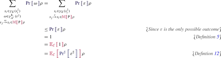
• Case $\omega ^\sharp = \mathbf {b}_{l}$:

  

• Case $\omega ^\sharp = \overline{\mathbf {b}}_{l}$:

  

• Case $\omega ^\sharp = \mathbf {u}^{i}_{l}$:

  

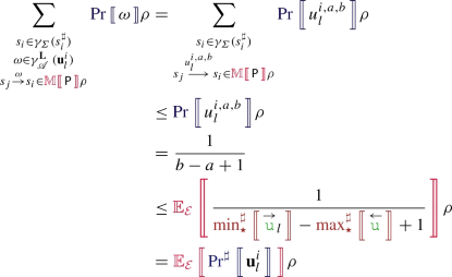
• Case :

  

• Case $\omega ^\sharp = \omega ^\sharp _0 \xi ^\sharp$:

  

• Case $\omega ^\sharp = {\omega ^\sharp }_1 + {\omega ^\sharp }_2$:

  

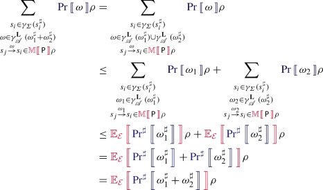
$\square$

Finally, using this lemma as an over-approximation of concrete scenario probabilities, we can derive from (4) the following:

$\square$

1.2 A.2 Normalization constraint

The second part of the theorem is the normalization constraint:

We have:

$\square$

B Benchmarks programs

See Fig. 17.

Fig. 17

Programs of the analyzed backoff mechanisms

References

Abate A, Katoen J-P, Lygeros J, Prandini M (2010) Approximate model checking of stochastic hybrid systems. Eur J Control 16(6):624–641
Anand S, Păsăreanu, CS, Visser W (2007) JPF-SE: a symbolic execution extension to Java Path Finder. In: TACAS’07, volume 4424 of LNCS. Springer, pp 134–138
Barthe G, Espitau T, Ferrer Fioriti L, Hsu J (2016) Synthesizing probabilistic invariants via Doob’s decomposition. In: CAV ’16, volume 9779 of LNCS. Springer, pp 43–61
Bouissou O, Goubault E, Goubault-Larrecq J, Putot S (2012) A generalization of p-boxes to affine arithmetic. Computing 94(2):189–201
Bouissou, O, Goubault E, Putot S, Chakarov A, Sankaranarayanan S (2016) Uncertainty propagation using probabilistic affine forms and concentration of measure inequalities. In: TACAS ’16, volume 9636 of LNCS. Springer, pp 225–243
Buchholz P (1994) Exact and ordinary lumpability in finite Markov chains. J Appl Probab 31(1):59–75
Chakarov A, Sankaranarayanan S (2013) Probabilistic program analysis with martingales. In: CAV ’13, volume 8044 of LNCS. Springer, pp 511–526
Chakarov A, Sankaranarayanan S (2014) Expectation invariants for probabilistic program loops as fixed points. In: SAS ’14, volume 8723 of LNCS. Springer, pp 85–100
Cousot P, Cousot R (1977) Abstract interpretation: a unified lattice model for static analysis of programs by construction or approximation of fixpoints. In: POPL ’77. ACM, pp 238–252
Cousot P, Halbwachs N (1978) Automatic discovery of linear restraints among variables of a program. In: POPL ’78. ACM, pp 84–97
Cousot P, Monerau M (2012) Probabilistic abstract interpretation. In: ESOP ’12, volume 7211 of LNCS. Springer, pp 169–193
Cousot R (1985) Fondements des méthodes de preuve d’invariance et de fatalité de programmes parallèles. Thèse d’État ès sciences mathématiques, Institut National Polytechnique de Lorraine, Nancy, France
Dattatreya GR (2008) Performance analysis of queuing and computer networks. Chapman and Hall/CRC, Boca Raton
Daws C (2004) Symbolic and parametric model checking of discrete-time Markov chains. In: ICTAC ’04, volume 3407 of LNCS. Springer, pp 280–294
De Loera JA, Hemmecke R, Tauzer J, Yoshida R (2004) Effective lattice point counting in rational convex polytopes. J Symb Comput 38(4):1273–1302
Dehnert C, Junges S, Jansen N, Corzilius F, Volk M, Bruintjes H, Katoen J.-P, Ábrahám E (2015) PROPhESY: a PRObabilistic ParamEter SYnthesis tool. In: CAV ’15, volume 9206 of LNCS. Springer, pp 214–231
Dubhashi DP, Panconesi A (2009) Concentration of measure for the analysis of randomized algorithms. Cambridge University Press, Cambridge
Feret J (2001) Abstract interpretation-based static analysis of mobile ambients. In: SAS ’01, volume 2126 of LNCS. Springer, pp 412–430
Ferson S, Kreinovick V, Ginzburg L, Sentz F (2003) Constructing probability boxes and Dempster-Shafer structures. Technical report, SAND2002-4015
Filieri A, Păsăreanu CS, Visser W (2013) Reliability analysis in symbolic pathfinder. In: ICSE ’13. IEEE Press, pp 622–631
Filieri A, Păsăreanu CS, Visser W, Geldenhuys J (2014) Statistical symbolic execution with informed sampling. In: FSE ’14. ACM, pp 437–448
Geldenhuys J, Dwyer MB, Visser W (2012) Probabilistic symbolic execution. In: ISSTA ’12. ACM, pp 166–176
Grimmett G, Stirzaker D (2001) Probability and random processes. Oxford University Press, Oxford
Grïßlinger A (2003) Extending the polyhedron model to inequality systems with non-linear parameters using quantifier elimination. Master thesis, University of Passau
Hahn E, Hermanns H, Zhang L (2011) Probabilistic reachability for parametric Markov models. Int J Softw Tools Technol Transf 13(1):3–19
Jeannet B, Miné A (2009) Apron: a library of numerical abstract domains for static analysis. In: CAV ’09, volume 5643 of LNCS. Springer, pp 661–667
Kemeney JG, Snell JL (1976) Finite Markov chains. Springer, Berlin
Kozen D (1985) A probabilistic PDL. J Comput Syst Sci 30(2):162–178
Kwiatkowska M, Norman G, Parker D (2011) PRISM 4.0: verification of probabilistic real-time systems. In: CAV ’11, volume 6806 of LNCS. Springer, pp 585–591
Le Gall T, Jeannet B (2007) Lattice automata: a representation for languages on infinite alphabets, and some applications to verification. In: SAS ’07, volume 4634 of LNCS. Springer, pp 52–68
Lesens D, Halbwachs N, Raymond P (2001) Automatic verification of parameterized networks of processes. Theor Comput Sci 256(1–2):113–144
Luckow K, Păsăreanu CS, Dwyer MB, Filieri A, Visser W (2014) Exact and approximate probabilistic symbolic execution for nondeterministic programs. In: ASE ’14. ACM, pp 575–586
McIver A, Morgan C (2004) Abstraction, refinement and proof for probabilistic systems. Monographs in Computer Science. Springer, Berlin
Miné A (2006) The octagon abstract domain. Higher Ord Symb Comput (HOSC) 19(1):31–100
Monniaux D (2000) Abstract interpretation of probabilistic semantics. In: SAS ’00, volume 1824 of LNCS. Springer, pp 322–339
Monniaux D (2001) Backwards abstract interpretation of probabilistic programs. In: ESOP ’01, volume 2028 of LNCS. Springer, pp 367–382
Monniaux D (2005) Abstract interpretation of programs as Markov decision processes. Sci Comput Program 58:179–205
Necula G, McPeak S, Rahul S, Weimer W (2002) CIL: intermediate language and tools for analysis and transformation of C programs. In: CC ’02, pp 213–228
Ouadjaout A, Miné A (2017) Quantitative static analysis of communication protocols using abstract Markov chains. In: SAS ’17, volume 10422 of LNCS. Springer, pp 277–229
Parikh R (1966) On context-free languages. J ACM 13(4):570–581
Puterman ML (1994) Markov decision processes: discrete stochastic dynamic programming. Wiley Series in Probability and Statistics. Wiley, Hoboken
Ross S (1996) Stochastic processes. Wiley, Hoboken
Sankaranarayanan S, Chakarov A, Gulwani S (2013) Static analysis for probabilistic programs: inferring whole program properties from finitely many paths. In: PLDI ’13. ACM, pp 447–458
Shafer G (1976) A mathematical theory of evidence. Princeton University Press, Princeton
Soudjani SEZ, Abate A (2014) Precise approximations of the probability distribution of a Markov process in time: an application to probabilistic invariance. In: TACAS ’14, volume 8413 of LNCS. Springer, pp 547–561 (2014)
Suriana P (2016) Fourier–Motzkin with non-linear symbolic constant coefficients. Master thesis, Massachusetts Institute of Technology
Van Hentenryck P, Cortesi A, Le Charlier B (1995) Type analysis of Prolog using type graphs. J Log Program 22(3):179–209
Venet A (1999) Automatic analysis of pointer aliasing for untyped programs. Sci Comput Program 35(2):223–248
Villemot S (2002) Automates finis et intérpretation abstraite: application à l’analyse statique de protocoles de communication. Rapport de DEA, École normale supérieure
Wang D, Hoffmann J, Reps T (2018) PMAF: an algebraic framework for static analysis of probabilistic programs. In: PLDI ’18. ACM, pp 513–528
Wolfram Research, Inc. (2017) Mathematica, Version 11.2, Champaign, IL
Author information
Authors and Affiliations
Corresponding author
Additional information
This work is partially supported by the European Research Council under Consolidator Grant Agreement 681393 – MOPSA.