
Abstract
Field data and simulation were used to investigate replication within trials and the allocation of replicates across trial sites using partial replication as an approach to improve the efficiency of early-stage selection in a potato breeding programme. Analysis of potato trial data using linear mixed models, based on four-plant (clonal) plots planted as augmented partially-replicated (p-rep) designs, obtained genetic and environmental components of variation for a number of yield and tuber components. Heritabilities, trial-to-trial genetic correlations and performance repeatability of clonal selections in p-rep trials and in subsequent fully replicated trial stages were high, and selection was effective for the economically important traits of marketable tuber yield and tuber cooking quality. Simulations using a parameter-based approach, pertaining to the variance components estimated from the p-rep field trials, and the parametric bootstrapping of historic empirical data showed improved rates of genetic gain with p-rep testing over one and two locations compared with testing in fully replicated trials. This potato breeding study suggests that the evaluation and selection of a clonal field crop in fully replicated trials may not be optimal in the early stages of a breeding cycle and that p-rep designs offer a more efficient and practical alternative.
Introduction
The initial stage of evaluation in a potato breeding programme comprises the visual assessment and phenotypic selection of single plants, or the evaluation and selection of families from formal progeny testing (Mackay 2007; Bradshaw et al. 2009). This is followed by more intense within-family selection from replicated clonal field trials. Traditionally, under these schemes there is a reliance on an adequate plant multiplication rate to allow entry of selected candidates into replicated field trials as early as possible. Potato, via the clonal propagation of tubers, has a relatively low multiplication rate that increases the generation interval and delays testing across multiple locations, slowing the rate of genetic progress and the time to deploy improved cultivars.
Replication demands a compromise between selection accuracy and the intensity of selection; increasing replication will improve the accuracy of genotype estimates but, with the reasonable assumption that the total number of available test plots or other test resources are fixed, the reduction in the number of tested candidates will affect the genetic response to selection. The precision and accuracy of assessment for genotype differences, along with their size and significance, are important considerations for advanced stage testing in breeding programmes and regional variety trials. Accuracy is desirable for early-stage trials also, but the emphasis at this stage is on the ranking of a large number of test entries. For early-stage evaluation, genotypes are often considered as random effects in a linear mixed model and their BLUPs (best linear unbiased predictions) are shrunk towards the population mean accordingly (Robinson 1991; Smith et al. 2005; Piepho et al. 2008). Under this evaluation framework, correlated data such as pedigree information and localised spatial field trends can be included for the prediction of breeding values and to enhance the accuracy of evaluations. This can be further extended to the multivariate analysis of trials over multiple locations.
Increasing the amount of information results in genotype predictions becoming less conservative and closer to their true values but previous work has indicated that under certain circumstances (e.g., a high proportion of genetic to phenotypic variance), greater genetic gain may be achieved by relaxing the demands for selection accuracy through planting fewer replicated genotypes and screening a greater number of unreplicated genotypes (Bos 1983; Gauch and Zobel 1996; Bos and Caligari 2008). Unreplicated trials provide breeders with an opportunity to test genotypes for quantitative characters, such as yield, in the early stages of a breeding programme before there are sufficient quantities of seed or seed tubers available for planting in replicated trials. Trial designs are often made up of the unreplicated candidate genotypes and a number of replicated controls or ‘checks’ that are used for error control (Kempton 1984). The use of augmented trial designs was first proposed by Federer (1956) in which replicated controls are allocated by randomisation into some form of systematic blocking arrangement, such as randomised complete block or row-column designs, and the remainder of the trial filled with unreplicated candidates. Checks are usually made up of a number of cultivar ‘standards’, but the use of these controls depletes the number of candidates that are available for selection and therefore potentially reduces the intensity of selection. To realise any improvement in selection efficiency, there has to be a substantial reduction in plot error when check frequency is high, particularly when heritabilities are high (Kempton 1984; Kempton and Gleeson 1997). To avoid the reduction of selection candidates due to check cultivars, Cullis et al. (2006) and Smith et al. (2006) described partially replicated (p-rep) designs in which all entries are selection candidates, with a proportion of the trial plots allocated to replicated candidates and the remaining plots filled with unreplicated candidates. This can be extended to multi-environment trial (MET) evaluation where a proportion of candidate genotypes can be replicated within and across trials. More recent studies have considered the design of augmented p-rep trials (Clarke and Stefanova 2011; Williams et al. 2011, 2014) and their performance in MET field trials (Moehring et al. 2014; Rattunde et al. 2015).
In New Zealand, the evaluation of historic potato field (replicated) trials at early selection stages has found high heritabilities of greater than 0.6 (as the proportion of genotypic or additive genetic variance to total phenotypic variance) for a number of yield and tuber traits, including total and marketable yields (Paget et al. 2015a) and tuber dry matter content (unpublished). Further, there is evidence to support the distribution of genetic material to multiple locations for MET evaluation in the early clonal stages as soon as possible (McCann et al. 2012). This has motivated the exploration of p-rep trials to increase early-stage selection efficiency in The New Zealand Institute of Plant & Food Research Limited (PFR) potato breeding programme, as previous observations suggest that full replication in early stage trials may not be optimal and slows the allocation of candidates for testing over multiple locations.
In this study, genetic parameters and the repeatability of clonal performance were measured, based on selections from augmented p-rep trials for tuber (marketable) yield and cooking (fry) quality. Variance components estimated from the p-rep trials provided the basis for inference from parameter-based simulations, allowing determination of the expected responses to selection. Evaluations of simulated data were over one or two ‘environments’ and used a linear mixed model with varying numbers of tested genotypes, heritabilities and genetic covariances for a single stage of selection. A second method of simulation, based on the assessment of historical trial data, used a parametric bootstrapping approach with trial analysis based on a formal p-rep design structure.
Materials and methods
Trial data
The genotypes tested were random selections from single-plant plots (clonal stage 1 or C1 trials) harvested in March 2011 at Lincoln, and were made up of 44 full-sib and 17 half-sib families. The selections were representative of genotypes screened as part of the PFR potato breeding programme. Field trials were planted for three consecutive years (2011, 2012 and 2013) at the Lincoln PFR research site in the South Island and for one year (2013) at the Pukekohe PFR research site in the North Island of New Zealand (Fig. 1). In the first season of field trials (2011–2012), a p-rep clonal stage 2 trial was designed using DiGGer (Coombes 2011), a Windows console program, by supplying an input file. The trial (LN-C2-11) was designed to be resolvable for the complement of replicated genotypes in two dimensions, i.e. across row-blocks and column-blocks (Fig. 2), and consisted of 236 entries and two check cultivars (‘Fraser’ and ‘Agria’) planted as four-tuber (four-by-one) plots. A p-rep trial was established again in the 2012–2013 season (LN-C2-12) with 200 of the same entries from the previous season and the same two checks. The target replication level of both C2 trials was p = 1.20 (where 20% of test entries are replicated), but the actual replication level in the first year was approximately p = 1.18 (18% of test entries were replicated) because of genotype attrition.

Principal trial locations for the PFR potato breeding programme, within New Zealand

Partially replicated (p-rep) potato trial with 1:196 unreplicated entries (grey, not labelled), 197:236 replicated entries (yellow) and two checks (237 (blue):238 (red)). (Color figure online)
From the p-rep LN-C2-11 (2011–2012) trial, 48 genotypes were randomly selected and planted in a fully replicated trial in the 2012–2013 season (LN-C3-12). A final year of fully replicated field trials was also carried out for the 48 genotype selections in the 2013–2014 season at both Lincoln (LN-C4-13) and Pukekohe (PK-C4-13). [Note that trials with the same number suffix were grown in the same season and corresponds to the year of planting; three consecutive seasons numbered 11 (2011–2012), 12 (2012–2013) and 13 (2013–2014)]. All Lincoln trials were planted in October and harvested in March the following year, approximately 150–160 days after planting. The Pukekohe trial was planted in October and harvested in late February approximately 140 days after planting. Fully replicated trials were designed as Latinized row-columns with CycDesigN v4.0 (CycSoftware 2009) and planted with three replicates in six-tuber (six-by-one) plots (Lincoln) and two replicates in twelve-tuber (six-by-two) plots (Pukekohe).
At harvest, plot yield was recorded for analyses, as a marketable tuber yield, which was the graded yield after undersized (less than 50 g) and defective tubers had been removed. Defective tubers, for example, may have been afflicted with secondary or abnormal growth, rot or excessive greening. Five tubers from each plot were also randomly sampled, chemically treated with sprout suppressant (Propham®) and stored at 10 °C. These tubers were removed from cold storage in September after 120 days and held for 24 h under ambient conditions (~17–19 °C). Potato slices (crisps) of ~1 mm thickness were then cooked by frying for 2 min at 190 °C in canola oil and scored on a 1–9 scale (Fig. 3) for fry score, with 1 indicating a high fry quality (light coloured, with no evidence of discolouration) and 9 indicating a very poor fry quality (blackened discolouration).

Potato fry colour assessment scale, where 1 displays very high quality (no discolouration) and 9 displays very poor quality (blackened discolouration). (Color figure online)
Statistical analysis of trial data
Trials were first analysed with a univariate linear mixed model, general form given by: y = X m + W b + Z g + e where y is the n × 1 vector of trait observations, m is a (p × 1) vector of fixed effects including the overall trial mean, b is a q × 1 vector of random non-genetic design factors, \(\user2{b}\sim N(0,{\mathbf{I}}\sigma _{b}^{2} )\), e.g. replicate and/or block (within replicate) and g is a (r × 1) vector of random genetic effects, \(\user2{g}\sim N(0,{\mathbf{I}}\sigma _{g}^{2} )\). The vector of random error terms is given by \(\user2{e}\sim N(0,{\mathbf{I}}\sigma _{{\text{e}}}^{2} )\) while X is a known n × p incidence matrix for the fixed effects, W (n × q) and Z (n × r) are known incidence matrices for the random effects, I are the relevant p × p, q × q and r × r identity matrices and the subscripted σ2 is the variance of each of the random effects. For each trait, analyses considered the blocking structure of the trial designs, allowing for independent random effects, such as blocks, and independent plot errors. For the LN-C2-11 and LN-C2-12 (p-rep) trials, check cultivars were fitted as fixed effects. There were no checks planted in trials LN-C3-12, LN-C4-13 and PK-C4-13. A fixed covariate was fitted in LN-C2-11 and LN-C2-12 to account for some waterlogging that had occurred for a short period over the duration of the trials. A fixed covariate was also fitted to account for the loss of plants in a small number of plots, but any plot with two plants or fewer was considered as a missing value. For tuber yield, a spatial model was tested by separating the random error term e into spatially dependent (autocorrelated) and spatially independent errors, following the AR1 spatial correlation model of Gilmour et al. (1997). A likelihood-ratio test was used as the criterion to test for the importance of the fitted spatial effects, which were retained as an addition to the trial blocking features if model fit was improved. The main emphasis for each univariate trial analysis was estimating the genotypic (total genetic) values of candidate varieties, i.e. the ‘production worth’ of varieties rather than their value as potential parents, but the prediction of breeding values was also considered. Therefore, data were also analysed after replacing the independent genotypic variance given by \({\mathbf{I}}\sigma _{g}^{2}\) with a pedigree-based genotypic variance given by \({\mathbf{A}}\sigma _{{\text{a}}}^{2}\), the variance–covariance matrix of the additive genetic effects (breeding values), where A is the numerator relationship matrix that provides the between-genotype relationship as two times the coefficient of coancestry. The pedigree was built from PFR field books and an online potato pedigree database (van Berloo et al. 2007). Variance component estimates provided an indication of the magnitude of signal-to-noise expected from p-rep potato trials and were used as basis to infer the expected response to selection using parameter-based simulations. In general, heritabilities were obtained from either the proportion of additive to phenotypic variance (h 2), or the proportion of genotypic to phenotypic variance (H 2, excluding the pedigree), with the phenotypic variance including the genetic, block/replicate and error variances. As variance components are unknown, the empirical genotypic (total genetic) and breeding values (EBVs) were obtained from the BLUPs of random effects (Henderson 1975). Coefficients of correlation were obtained for the performance of the 48 genotypes common between C2 and C3 trials, based on their BLUPs of genetic and breeding values.
The univariate model was also extended to a multivariate analyses of MET data for the five trials, LN-C2-11, LN-C2-12, LN-C3-12, LN-C4-13 and PK-C4-13. Random effects were assumed to follow a multivariate normal distribution with means and variances defined by:
where 0 are null matrices. B 0, G 0 and R are covariance matrices for design factors, genetic (additive) and residual effects, respectively, and \({\mathbf{ \otimes }}\) is the direct (Kronecker) product. The matrix B 0 is a diagonal matrix of (non-genetic) scaled identity matrices. The variance–covariance structure of plot error effects R is assumed to be block diagonal and specified as a separable AR1 process to account for local spatial trend as in the single trial analysis, with the independent error variance for each trial. The unstructured (US) genetic variance–covariance matrix was approximated using a factor analytic (FA) approach as outlined by Smith et al. (2001) with separate residual variances modelled for each trial. The FA method aims to reduce the rank of the genetic covariance matrix in multivariate analysis and is considered a parsimonious approximation to the US genetic (co)variance matrix. It assumes that t trials (or traits) are linear combinations of a few latent variables (the common factors that bring about the correlations between variables) and any variance not explained by these common factors is fitted separately as trial specific factors: \({\mathbf{G}}_{0} = {\text{ }}{\mathbf{\Lambda \Lambda }}^{\prime } + {\mathbf{S}}\); where \(\mathbf{\Lambda}\) is a (t × k) matrix of factor loadings:
and S is a (t × t) diagonal matrix of specific variances. Genetic variances and covariances were estimated simultaneously from an FA model of order 2 for the same trait measured in different trials or ‘environments’ (locations and/or years) and the estimate of trial–trial genetic correlations, also known as Type B genetic correlations (Yamada 1962; Burdon 1977), for each trait. Further details of FA models can be found in Smith et al. (2001) and Meyer (2009). Data were analysed using R (R Development Core Team 2012) and ASReml-R (Butler 2009; Butler et al. 2009).
Simulation of genetic response: parameter-based simulation
The first approach to simulation used a stochastic, parameter-based method to model selection in replicated and p-rep trials over both one and two locations for a single clonal selection stage. In predicting the response to selection, it was assumed that the trait under consideration was normally distributed. Normal distributions of true genotypic values (g) and environmental deviations were obtained from given estimates of genetic and environmental variances, and these were used to produce a simulated breeding population. In this case, the vector of additive effects a and non-additive effects d were assumed to be mutually independent, so that the vector of total genetic effects (g = a + d) had distribution \(\user2{g}\sim N(0,\sigma _{a}^{2} {\mathbf{I}} + \sigma _{d}^{2} {\mathbf{I}})\). Alternatively, the additive and non-additive effects could be sampled independently from separate distributions when assuming no covariance between additive and non-additive genetic effects. In the present study, the difference between the two sampling strategies is likely to be small, but independent sampling allows for greater flexibility, e.g., allowing for additive genetic covariances between related individuals, if a pedigree structure is incorporated, and including dominance as a separate component. For p-rep trials, the level of replication was set at 25% (p = 1.25), which was compared with selection from fully replicated trials with two replicates (p = 2). Assuming that the genetic values for the trait were polygenic, the phenotypic variance was arbitrarily set at 10, with heritability varying from 0.1 to 0.8, giving an equivalent signal-to-noise ratio \(\sigma _{g}^{2} /\sigma _{e}^{2}\) that ranged from 0.11 to 4.0 (Table 1). For selection over two locations, the sampling of genetic values was from a multivariate normal distribution with the same genetic variances and genetic correlations of 0.2, 0.5 and 0.8. The sites were assumed to be equally weighted so that the true genotypic value for each individual was the mean of the sampled genotypic values. Four test scenarios (a, b, c and d) were simulated for each of p = 1.25 and p = 2:
-
a.
Single location testing, fixed number of total plots (nP) of 100 (to correspond approximately with simulation using historical field data; see next section ‘Bootstrap resampling using historic empirical data’) and
-
b.
As (a), but with nP of 1000.
-
c.
Extension of (b) with testing over two locations for both p = 1.25 and p = 2, with nP of 2000 in each of two locations to test 1600 genotype entries (p = 1.25) and 1000 genotype entries (p = 2).
-
d.
nP of 2000, distributed over one (p = 2) or two (p = 1.25) locations. The replication level at p = 1.25 to test 800 genotype entries (1000 plots in each of two locations) is shown in Table 2. Testing at p = 2 at one location (2000 plots) allows 1000 genotypes in total to be tested.
Table 2 Replication level for p = 1.25 over two locations, fixed number of total plots = 2000 testing 800 genotypes (scenario d)
For each scenario, data were generated for 10,000 simulations and analysed using a linear mixed model in ASReml-R (Butler 2009) to obtain predictions of the empirical genotypic values. The top performing individuals resulting from the analyses, comprising 5, 10 or 20% of the total genotypes tested (s), were selected based on the ranking of their empirical genotype values. The selection response was considered to be the difference between the mean true genotypic values of the s individuals and the mean of the true genotypic values of the breeding population. Therefore, truncation selection over a single cycle on a single trait was applied and the selection intensity was obtained directly from the proportion of genotypes selected when p = 1.25 for scenarios a, b and c, and p = 2 for scenario d. A relative genetic response to selection (ΔG′) was also calculated for p-rep tested genotypes (relative to the response when p = 2 so that ΔG′ = RP/R, where RP is the p-rep selection response and R is the fully replicated selection response) and stored for each simulation run.
Simulation of genetic response: bootstrap resampling using historic empirical data
The second approach was an empirically based simulation that aimed to take into account the error structure from historical field data and overlay a formal p-rep design on the original replicated trial. The field data were based on early-stage C2 potato yield trials from Pukekohe, grown between 1999 and 2012, and consisted of small, multiple α-Latinized designs (80–100 genotypes per trial) of two replicates, with each plot made up of 12 tubers grown in a six-by-two row arrangement. The bootstrap simulation is outlined as follows:
-
1.
The replicated trial was analysed using a linear mixed model in ASReml-R (Butler 2009), following the general form of the univariate model outlined in the section Statistical analysis. Genotypes were considered to be random effects and the overall mean fitted as a fixed effect. The residuals from this analysis were used to give the spatial layout of the environmental effects for subsequent p-rep analyses for each trial. The best linear unbiased predictions of genotypic values for tested genotypes were obtained from the solutions of the mixed model equations using the estimated variance parameters. The resulting empirical genetic values (eGVs) were considered to be the actual genetic values (aGVs) for the simulations.
-
2.
A minimal level of p-rep, Pmin, was elected to be 1.15, and therefore the standard p-rep trial size was Ng × Pmin where Ng = number of genotypes in the replicated trial. For example, a replicated C2 trial of 160 plots would comprise 80 genotypes and so a p-rep analysis of this particular trial would be 80 × 1.15 = 92 plots in total for all levels of partial replication. Levels of p-rep (p) greater than 1.15 therefore required the random elimination of some genotypes for each analysis, as increasing replication would not allow the full complement of genotypes to be assessed at any one time over a fixed number of plots (see Table 3).
Table 3 Example of the expected number of total genotypes, replicated genotypes and total plots available for p-rep simulation at different levels of p-rep (p) using the empirical data from an historic replicated trial (step 2) with a total of 160 plots and 80 genotypes. At a minimum p of 1.15, the total number of plots available for simulation is 92. Higher levels of p therefore require a random elimination of genotypes for each set of simulated data -
3.
For each level of p-rep, p, a trial was designed using trial design software DiGGer (Coombes 2011) in statistical software R (R Development Core Team 2012). The trial was designed to be resolvable, for the complement of replicated genotypes, in two dimensions (i.e. across row-blocks and column-blocks). This design was randomly located over the replicated C2 trial with associated plot residuals (as initially computed in step 1) allocated to the new layout. Genotypes were then randomly allocated to the treatment numbers of the trial design created. For computing expedience, designs were used several times by transformation, e.g., rotation, reflection.
-
4.
For each plot, a simulated genetic value was generated from the parametric bootstrap of the genetic value (pbGV) for the genotype plus the plot residual (environmental) effect for its location in the trial (Fig. 4). The pbGV was obtained by adding random noise taken from a normal distribution with mean = 0 and standard deviation = SE to the aGV, where SE is the standard error of the eGV as obtained from the replicated C2 analysis in 1.
Fig. 4 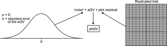
A simulated genetic value (pbGV) for a genotype in each plot was generated (step 4) by adding the plot residual from its particular location in the trial and the random noise, taken from a normal distribution with mean = 0 and the standard deviation = the standard error of the empirical genetic value (eGV), to the actual genetic value (aGV). The eGVs (= aGVs) and plot residuals were obtained from the replicated trial analysis (step 1)
-
5.
The data generated were then analysed in ASReml-R (Butler 2009) following the general form of the univariate linear mixed model as described in section Statistical analysis. A response to selection ΔG, and relative response to selection, ΔG′ were calculated and stored for each simulation run following the ‘parameter-based simulation’ approach as outlined, a method previously described by Piepho and Möhring (2007). Only marketable yield, as the character of most interest, was tested. There were a total of 5000 simulation runs for each p.

Results
Field trials
Variance components and broad-sense heritability (H 2) estimates for the p-rep trials LN-C2-11 and LN-C2-12 are presented in Table 4. Estimates of narrow-sense heritabilities were very similar (results not shown). Spatial correlations were much higher for LN-C2-12 than for LN-C2-11 for tuber yield. This may have been due to soil compaction, which was observed in some areas of the trial, causing spatial patchiness because of periods of waterlogging (or as a result of poorer root development because of soil panning) during the growing season. A significant fixed covariate (p < 0.05) fitted for the analysis of tuber yield trait in LN-C2-12 to account for the worst affected area disappeared when spatial effects were fitted. This contrasts with LN-C2-11, in which both a fixed covariate (p < 0.05) and spatial effects were fitted. The waterlogging in this trial was only found in rows one to two (Fig. 2) but there was a greater weed burden throughout the trial which also may have contributed to the spatial heterogeneity.
Correlations of genotypic values estimated (data not shown) from univariate analysis for LN-C2-11 and LN-C3-12 (between subsequent selection stages and seasons), were high for the two traits considered (0.78 for tuber yield and 0.70 for fry score). These were very similar to the correlations between EBVs (0.80 and 0.68 respectively), which are displayed in Fig. 5, illustrating the strong relationship between stages LN-C2-11 and LN-C3-12. Correlations between genotypic values for C2 and C3 grown in the same year (LN-C2-12, LN-C3-12) were at least as high (0.78 for tuber yield) or higher (0.82 for fry score) than correlations between C2 and C3 grown in different years (LN-C2-11, LN-C3-12). Differences may have been due to both seasonal effects and carry-over, or ‘maternal’, effects for tuber yield, from growing test plots at the C2 stage with tubers selected from single plants for each genotype. Trial-to-trial genetic correlations estimated from multivariate FA analysis using MET data (C2 and C3 trials at Lincoln and C4 trials at both Lincoln and Pukekohe) found consistently high correlations for tuber yield (mostly >0.8) and a greater range for fry score (0.57 to 0.93). These are shown in Fig. 6.

Correlation of empirical breeding values (EBVs) between p-rep (LN-C2-11) and fully replicated (LN-C3-12) field trials for; a tuber (marketable) yield and; b tuber fry score. Graphs show the line of unity

Trial-to-trial genetic correlation estimates from factor analytic models for tuber (marketable) yield and tuber fry score. (Color figure online)
Parameter and empirical-based simulations
At a selection proportion (s) of 5% with 100 tested genotypes at a single location (scenario a), parametric-based simulation showed that the relative selection response was close to unity when h 2 (or H 2) ≈0.4–0.5 (Fig. 7a). The relative response reduced slightly at all levels of s (5, 10 and 20%) with 1000 tested genotypes (Fig. 7b). There was some evidence to suggest that relative gain was overestimated with small sample sizes and at low heritabilities, possibly because of difficulties in estimating variance components. At s = 20, there was no advantage in replicating trials. When testing over two locations with both full replication and p-rep (scenario c) at a selection proportion of 5%, relative response was at unity at a heritability of just over 0.30 when the trial-to-trial genetic correlation was high (0.80) and just over 0.40 when the genetic correlation was low (Fig. 7c). This reduction in heritability when Rp/R = 1 compared with scenario a is expected, given that some genotypes were replicated three times (four times when p = 2) over the two locations. The relative responses to selection for all correlations did not surpass 1.10 and tended to converge as heritability approached 0.80. Relative response easily offset the reduction in the number of p-rep genotypes tested over two locations, even at very low heritabilities (Fig. 7d). The advantage of testing over two locations when trial-to-trial correlations are high was generally small however, with the relative response trending towards unity as heritability increases, although Rp/R was greater than 1 for all heritabilities tested.

Simulation of the relative response to selection (Rp/R) at increasing heritabilities (where Rp is the p-rep selection response and R is the fully replicated selection response); where a testing in one location, 100 total plots and 5, 10 and 20% proportion selected (s); b as a but with 1000 total plots; c testing in two locations with 2000 total plots (in each location) with genetic correlations (r) between locations of 0.2, 0.5 and 0.8 and s = 5; d testing in one location (full replication), 1000 genotypes, 2000 total plots and s = 5, or testing in two locations (p-rep), 800 genotypes and 2000 total plots (1000 in each location), s = 5 and genetic correlations as in c
Table 5 shows an example of a bootstrap simulation run (5000 samples) at all levels of tested p-rep using historical field data, with a target number of test plots set at 92. The total number of genotypes tested at p = 1.25 was approximately 75, which reduced to 46 at p = 2. Trials presented in Table 6 are a representative set of trials, with regard to heritabilities, from years 1999 to 2012 for tuber yield, with the lowest and highest heritabilities found in trials C2-06A and C2-99D/C2-00B respectively. For trial C2-12E, H 2 = 0.46 and the relative response was close to one at s = 5, which was similar to the result from parametric-based simulation (Fig. 7a). For trial C2-06B, H 2 = 0.66 and the relative response was 1.35 at s = 0.20, which was inflated well above that expected, given the results of the parametric-based simulation at this heritability (Fig. 7a). There were few Pukekohe trials with heritabilities of less than 0.4 for tuber yield with records available, and so there was limited opportunity to test the empirical simulations at low heritabilities. An exception was the C2-06A trial, where the heritability of tuber yield was estimated to be 0.25. At p-rep = 1.25, simulation of this trial gave a relative selection response of 0.93 for s = 5 and 1.05 for s = 10. From parametric-based simulation results, unity of relative selection response (Rp/R = 1) for s = 10 was expected at an approximate heritability of 0.3. Again, the relative selection response appeared to be inflated above expectation, when s = 20.
Discussion
Reducing the degree of clonal replication within field trials is motivated by two main factors: i) the relatively low multiplication rate of potato tubers, i.e., a shortage of planting material in the early stages of breeding programmes and therefore the time lag associated with entering candidates into formal trial evaluation including MET testing, and ii) a desire to increase the number of candidates tested (when the total number of plots is fixed and it is assumed that the phenotyping of extra candidates is not constrained). The results are presented in terms of genetic gain, whilst acknowledging that the motives and constraints of implementing a selection scheme will vary with the specific programme.
Empirical and simulated data
For the potato traits presented, the results using both empirical and simulated data indicate that increased genetic gain could be achieved in a potato breeding programme by applying p-rep trial evaluation at the early stages of selection. Concordance of genetic values between subsequent clonal stages, after selection from p-rep trials, were mostly high to moderately high for important economic traits, marketable tuber yield and fry quality. In Scotland, work by Caligari et al. (1986) found a correlation coefficient of phenotypic performance for total tuber yield between the second (C2) and third (C3) clonal stages of 0.52. These were tested over two locations and there was no significant clone × location interaction. A correlation coefficient of 0.78 (genotypic value) for marketable tuber yield at a single location was found in the present study.
Given the heritabilities reported, previous work based on order statistics and known selection formulae also indicate that the expected genetic gain at moderate to high heritabilities may be greater at a single location by planting fewer replicated entries (Bos 1983; Gauch and Zobel 1996). This moderates the selection accuracy but the trade-off is in allowing more genotypes to be tested (Bos 1983). From Fig. 7a, b the relative selection response was close to unity when h 2 (or H 2) ≈0.4–0.5, which was similar to that predicted for unreplicated testing using a deterministic approach by Bos (1983). The recommendations of Gauch and Zobel (1996) were more conservative, suggesting that unreplicated testing was suitable when h2 = 0.6 and greater, when the total number of plots was 100. At 1000 plots, two replicates were favoured when h2 was 0.75, the maximum shown. This work accounted for the extra noise generated by testing more plots, so that increasing the number of genotypes tested had the desirable effect of increasing the number of superior genotypes, but also the undesirable consequence of adding more noise (inferior genotypes). There was only a small indication of this trade-off in the present study, as the relative response reduced slightly at all levels of s with 1000 test plots (Fig. 7b) compared with 100 test plots (Fig. 7a). Cullis et al. (2006) and Piepho and Möhring (2007) have emphasised that under more complex analysis, for example when data are unbalanced and genotypic effects are correlated, it is not appropriate to apply the standard measures of heritability to compute a response to selection. An alternative approach, proposed by Piepho and Möhring (2007), measured selection response directly using a simulation-based method, thus avoiding the necessity to define the heritability or to use an altogether inappropriate measure of heritability. This simulation approach was also applied in the present study, based on empirical data from clonal stage 2 yield trials. Results from parameter-based simulations found an increase in the expected response to selection at the intensities that are typically employed in the early stages of a clonal selection scheme when testing at a single location in p-rep trials.
Early-stage testing in multiple locations
The results from simulation also showed that selection over two locations in p-rep trials may be particularly beneficial compared with selection over one location in a fully replicated trial, when locations are weighted equally in a selection index, i.e., selection is for broad adaptation. The advantages, particularly for low trial-to-trial correlations, are clearly seen in Fig. 7d. Only positive correlations between locations were considered in this study, as negative correlations have not been found in previous analyses of PFR breeding scheme MET data for tuber yield traits (Paget et al. 2015b). Negative correlations indicate a greater importance of qualitative G × E interactions, and that separate selection schemes targeting specific adaptations in localised regions may be required, e.g. Atlin et al. (2000), Windhausen et al. (2012).
For METs, the precision of across-trial comparisons is compromised in the presence of G × E effects. The magnitude of estimated average G × E variances for yield in a number of different crops has previously been reported (Talbot 1984). For potato, this was found to be greater than the within-trial plot variances, and so efforts expended on maximising selection precision by replication at an individual trial site may be wasted (Kempton and Gleeson 1997). At low heritabilities, the advantage of extending p-rep testing to two locations is maintained over full replication at a single location (scenario d), particularly for low trial-to-trial correlations (Fig. 7d) and despite a reduction in the number of candidates tested with a fixed number of total plots available. This is a more realistic scenario than scenario c at the C2 stage of selection, because of the shortage of available planting material. The advantage of testing over two locations when trial-to-trial genetic correlations are high is not so obvious however, with the relative response trending towards unity as heritability increased. Managing trials over two or more locations may become more difficult to justify in this case, with the difference in gain (which was less than 1%) having to be measured against the extra costs incurred, but this is beyond the scope of the present study. Unreplicated or p-rep trials offer a means to increase the number of test genotypes over a fixed number of plots or, alternatively, a means to reduce the number of plots to test an equivalent number of genotypes which may maximise gain per unit cost (e.g. Stendal and Casler 2006). With molecular information, Moreau et al. (2000) found that unreplicated trials were optimal for marker-assisted selection as well as phenotypic selection when traits were sensitive to G × E effects. Lorenz (2013) simulated resource allocation under genomic selection and favoured increasing population size rather than replication. For tuber yield, previous analyses of PFR early stage trials at Pukekohe have shown that heritabilities are generally high and that genetic correlations between adjacent seasons are also usually high (>0.70). This may not be the case for all traits, as fry quality has been reported to show significant G × E interaction effects (Affleck et al. 2008), which was similarly found by Hayes and Thill (2003), who recommended that genotypes should be tested for fry quality over multiple locations. Genetic parameters obtained for fry score in the present study, including trial-to-trial genetic correlations estimated from a FA model using MET data, indicated that evaluation in p-rep trials would be appropriate. Moehring et al. (2014) demonstrated that unreplicated and augmented p-rep trials outperformed augmented and fully replicated trials in MET evaluation of triticale and maize. They reported that p-rep trials were slightly inferior to unreplicated trials but had advantages including the possibility of single trial analysis. Like Talbot (1984), allocating replicates to multiple environments and decreasing the number of replicates in each environment was recommended. In potato, McCann et al. (2012) found that maximising replication of smaller plots over several locations and/or years rather than increasing replication at a single location improved the precision of genotype differences for several tuber quality traits including fry colour, sugar content and dry matter. Haynes et al. (2012) recommended the distribution of tubers to multiple test locations in the eastern USA at the early selection stages as an approach to select parents that produce more broadly-adapted progenies.
Conclusions
P-rep trials provide an opportunity to increase the number of genotypes that are tested in a single site and also allow an extension of trials to multiple locations for MET testing at an earlier stage than is currently practised. Based on empirical trials and simulation, results indicate that p-rep trials in a potato improvement programme will increase the rate of genetic gain for tuber yield and quality components. Further advantages are possible if material can be distributed across trial sites, i.e., multiple locations, at an earlier stage than is possible with full replication. It is concluded that full replication at the early stages in a selection programme may be sub-optimal and the use of p-rep designs should be considered as a means to improve the selection efficiency of potato breeding.
References
Affleck I, Sullivan JA, Tarn R, Falk DE (2008) Genotype by environment interaction effect on yield and quality of potatoes. Can J Plant Sci 88:1099–1107
Atlin GN, Baker RJ, McRae KB, Lu X (2000) Selection response in subdivided target regions. Crop Sci 40:7–13
Bos I (1983) Optimum number of replications when testing lines or families on a fixed number of plots. Euphytica 32:311–318
Bos I, Caligari PDS (2008) Selection methods in plant breeding, 2nd edn. Springer, Dordrecht
Bradshaw J, Dale M, Mackay G (2009) Improving the yield, processing quality and disease and pest resistance of potatoes by genotypic recurrent selection. Euphytica 170:215–227. doi:10.1007/s10681-009-9925-4
Burdon RD (1977) Genetic correlation as a concept for studying genotype-environment interaction in forest tree breeding. Silvae Genet 26:168–175
Butler D (2009) asreml: asreml() fits the linear mixed model. R package v.3.0-1. www.vsni.co.uk
Butler DG, Cullis BR, Gilmour AR, Gogel BJ (2009) ASReml-R reference manual, VSN International, Hemel Hempstead, UK, www.vsni.co.uk
Caligari PDS, Brown J, Abbott RJ (1986) Selection for yield and yield components in the early generations of a potato breeding programme. Theor Appl Genet 73:218–222
Clarke GPY, Stefanova KT (2011) Optimal design for early-generation plant breeding trials with unreplicated or partially replicated test lines. Australian & New Zealand Journal of Statistics 53:461–480
Coombes N (2011) DiGGer design generator under correlation and blocking. http://www.austatgen.org/software. Accessed: 31 January 2016
Cullis BR, Smith AB, Coombes NB (2006) On the design of early generation trials with correlated data. J Agric Biol Environ Stat 11:381–393
CycSoftware (2009) CycDesigN 4.0 A package for the computer generation of experimental designs. Version 4.0, CycSoftware Ltd, Hamilton, New Zealand. www.vsni.co.uk
Federer WT (1956) Augmented (or hoonuiaku) designs. Hawaiian Planter’s Record 55:191–208
Gauch HG, Zobel RW (1996) Optimal replication in selection experiments. Crop Sci 36:838–843
Gilmour AR, Cullis BR, Verbyla AP, Gleeson AC (1997) Accounting for natural and extraneous variation in the analysis of field experiments. J Agric Biol Environ Stat 2:269–293
Hayes RJ, Thill CA (2003) Genetic gain from early generation selection for cold chipping genotypes in potato. Plant Breed 122:158–163. doi:10.1046/j.1439-0523.2003.00776.x
Haynes KG, Gergela DM, Hutchinson CM, Yencho GC, Clough ME, Henninger MR, Halseth DE, Sandsted E, Porter GA, Ocaya PC (2012) Early generation selection at multiple locations may identify potato parents that produce more widely adapted progeny. Euphytica 186:573–583. doi:10.1007/s10681-012-0685-1
Henderson CR (1975) Best linear unbiased estimation and prediction under a selection model. Biometrics 31:423–449
Kempton RA (1984) The design and analysis of unreplicated field trials. Vortrage fur Pflanzenzuchtung 7:219–242
Kempton RA, Gleeson AC (1997) Unreplicated trials. In: Kempton RA, Fox PN (eds) Statistical methods for plant variety evaluation. Chapman & Hall, London, pp 86–100
Lorenz AJ (2013) Resource allocation for maximizing prediction accuracy and genetic gain of genomic selection in plant breeding: a simulation experiment. G3-Genes Genomes. Genetics 3:481–491
Lynch M, Walsh B (1998) Genetics and analysis of quantitative traits. Sinauer Associates Inc., Sunderland
Mackay G (2007) Propagation by traditional breeding methods. Potato. In: Razdan MK, Mattoo A (eds) Genetic improvement of Solanaceous crops. Enfield Science Publishers, Enfield, pp 65–81
McCann LC, Bethke PC, Casler MD, Simon PW (2012) Allocation of experimental resources used in potato breeding to minimize the variance of genotype mean chip color and tuber composition. Crop Sci 52:1475–1481. doi:10.2135/cropsci2011.07.0392
Meyer K (2009) Factor-analytic models for genotype x environment type problems and structured covariance matrices. Genet Sel Evol. doi:10.1186/1297-9686-41-21
Moehring J, Williams ER, Piepho HP (2014) Efficiency of augmented p-rep designs in multi-environmental trials. Theor Appl Genet 127:1049–1060. doi:10.1007/s00122-014-2278-y
Moreau L, Lemarie S, Charcosset A, Gallais A (2000) Economic efficiency of one cycle of marker-assisted selection. Crop Sci 40:329–337
Paget MF, Alspach PA, Anderson JAD, Genet RA, Apiolaza LA (2015a) Trial heterogeneity and variance models in the genetic evaluation of potato tuber yield. Plant Breed 134:203–211. doi:10.1111/pbr.12251
Paget MF, Apiolaza LA, Anderson JAD, Genet RA, Alspach PA (2015b) Appraisal of test location and variety performance for the selection of tuber yield in a potato breeding program. Crop Sci 55:1957–1968. doi:10.2135/cropsci2014.11.0801
Piepho HP, Möhring J (2007) Computing heritability and selection response from unbalanced plant breeding trials. Genetics 177:1881–1888. doi:10.1534/genetics.107.074229
Piepho HP, Möhring J, Melchinger AE, Büchse A (2008) BLUP for phenotypic selection in plant breeding and variety testing. Euphytica 161:209–228. doi:10.1007/s10681-007-9449-8
R Development Core Team (2012) R: a language and environment for statistical computing. In: R Foundation for Statistical Computing, Vienna, Austria
Rattunde HFW, Michel S, Leiser WL, Piepho HP, Diallo C, vom Brocke K, Diallo B, Haussmann B, Weltzien E (2015) Farmer participatory early-generation yield testing of sorghum in West Africa: possibilities to optimise genetic gains for yield in farmers’ fields. Crop Sci 56:2493–2505. doi:10.2135/cropsci2015.12.0758
Robinson GK (1991) That BLUP is a good thing: the estimation of random effects. Stat Sci 6:15–32
Smith AB, Cullis BR, Thompson R (2001) Analyzing variety by environment data using multiplicative mixed models and adjustments for spatial field trend. Biometrics 57:1138–1147. doi:10.1111/j.0006-341X.2001.01138.x
Smith AB, Cullis BR, Thompson R (2005) The analysis of crop cultivar breeding and evaluation trials: an overview of current mixed model approaches. J Agric Sci 143:449–462. doi:10.1017/s0021859605005587
Smith AB, Lim P, Cullis BR (2006) The design and analysis of multi-phase plant breeding experiments. J Agric Sci 144:393–409. doi:10.1017/s0021859606006319
Stendal C, Casler MD (2006) Maximizing efficiency of recurrent phenotypic selection for neutral detergent fiber concentration in smooth bromegrass. Crop Sci 46:297–302. doi:10.2135/cropsci2005.0083
Talbot M (1984) Yield variability of crop varieties in the UK. J Agric Sci 102:315–321
van Berloo R, Hutten RCB, van Eck HJ, Visser RGF (2007) An online potato pedigree database resource. Potato Res 50:45–57
Williams E, Piepho HP, Whitaker D (2011) Augmented p-rep designs. Biom J 53:19–27. doi:10.1002/bimj.201000102
Williams ER, John JA, Whitaker D (2014) Construction of more flexible and efficient p-rep designs. Aust NZ J Stat 56:89–96
Windhausen VS, Wagener S, Magorokosho C, Makumbi D, Vivek B, Piepho HP, Melchinger AE, Atlin GN (2012) Strategies to subdivide a target population of environments: results from the CIMMYT-led maize hybrid testing programs in Africa. Crop Sci 52:2143–2152. doi:10.2135/cropsci2012.02.0125
Yamada Y (1962) Genotype by environment interaction and the genetic correlation of the same trait under different environments. Jpn J Genet 37:498–509. doi:10.1266/jjg.37.498
Acknowledgements
We would like to thank Moe Jeram for the management of the Pukekohe field trials. We thank Satish Kumar and Steve Lewthwaite for helpful suggestions that improved the manuscript. We also gratefully acknowledge the funding assistance for this study provided by Potatoes NZ Charitable Trust.
Author information
Authors and Affiliations
Corresponding author
Rights and permissions
About this article

Cite this article
Paget, M.F., Alspach, P.A., Anderson, J.A.D. et al. Replicate allocation to improve selection efficiency in the early stages of a potato breeding scheme. Euphytica 213, 221 (2017). https://doi.org/10.1007/s10681-017-2004-3
Received:
Accepted:
Published:
DOI: https://doi.org/10.1007/s10681-017-2004-3