The Exponentiated Hencky-Logarithmic Strain Energy. Part I: Constitutive Issues and Rank-One Convexity

Abstract

We investigate a family of isotropic volumetric-isochoric decoupled strain energies

$$\begin{aligned} F\mapsto W_{\mathrm{eH}}(F):=\widehat{W}_{\mathrm{eH}}(U):=\left \{ \begin{array}{l@{\quad}l} \frac{\mu}{k} e^{k\|\operatorname {dev}_n\log{U}\|^2}+\frac{\kappa}{{2 {\widehat {k}}}} e^{\widehat{k}[\operatorname {tr}(\log U)]^2}&\text{if}\ \det F>0,\\ +\infty&\text{if}\ \det F\leq0, \end{array} \right . \end{aligned}$$

based on the Hencky-logarithmic (true, natural) strain tensor logU, where μ>0 is the infinitesimal shear modulus, $\kappa=\frac{2\mu+3\lambda}{3}>0$ is the infinitesimal bulk modulus with λ the first Lamé constant, $k,\widehat{k}$ are additional dimensionless material parameters, F=∇φ is the gradient of deformation, $U=\sqrt{F^{T} F}$ is the right stretch tensor and is the n-dimensional deviatoric part of the strain tensor logU. For small elastic strains, W _eH approximates the classical quadratic Hencky strain energy

$$\begin{aligned} F\mapsto W_{\mathrm{H}}(F):=\widehat{W}_{\mathrm{H}}(U)&:={\mu}\| \operatorname {dev}_n\log U\|^2+\frac{\kappa}{2}\bigl[\operatorname{tr}( \log U)\bigr]^2, \end{aligned}$$

which is not everywhere rank-one convex. In plane elastostatics, i.e., n=2, we prove the everywhere rank-one convexity of the proposed family W _eH, for $k\geq\frac{1}{4}$ and $\widehat{k}\geq\frac{1}{8}$. Moreover, we show that the corresponding Cauchy (true)-stress-true-strain relation is invertible for n=2,3 and we show the monotonicity of the Cauchy (true) stress tensor as a function of the true strain tensor in a domain of bounded distortions. We also prove that the rank-one convexity of the energies belonging to the family W _eH is not preserved in dimension n=3 and that the energies

$$\begin{aligned} F\mapsto\frac{\mu}{k}e^{k\|\log U\|^2},\qquad F\mapsto\frac{\mu }{k}e^{\frac{k}{\mu} \bigl(\mu\|\operatorname {dev}_n\log U\|^2+\frac{\kappa}{2}[\operatorname {tr}(\log U)]^2 \bigr)}, \quad F \in\mathrm{GL}^+(n), n\in \mathbb {N}, n\geq2 \end{aligned}$$

are also not rank-one convex.

1 Introduction

1.1 Logarithmic Strain and Geodesically Motivated Invariants

We introduce a modification of the well-known isotropic quadratic Hencky strain energy

$$W_{{\mathrm{H}}}(F) = \widehat{W}_{{\mathrm{H}}}(U) = {\mu}\|\operatorname {dev}_n\log U\|^2+\frac{\kappa}{2}\bigl[\operatorname {tr}(\log U) \bigr]^2 , $$

where μ>0 is the infinitesimal shear (distortional) modulus, $\kappa=\frac{2\mu+3\lambda}{3}>0$ is the bulk modulus with λ the first Lamé constant, F=∇φ is the deformation gradient, $U=\sqrt {F^{T} F}$ is the right Biot stretch tensor, logU is the referential (Lagrangian) logarithmic strain tensor, ∥ . ∥ is the Frobenius tensor norm, and is the n-dimensional deviatoric part of a second order tensor $X{\in \mathbb {R}^{n\times n}}$ (see Sect. 2 for other notations).

It was recently discovered [170, 171] (see also [32, 132]) that the Hencky strain energy enjoys a surprising property, which singles it out among all other isotropic strain energy functions. Indeed, the Hencky energy measures the geodesic distance of the deformation gradient F∈GL⁺(n) to the special orthogonal group SO(n), i.e.,

$$\begin{aligned} \begin{aligned} &\operatorname {dist}^2_{\mathrm{geod}}\bigl(F, \mathrm {SO}(n)\bigr) = {\mu} \|\operatorname {dev}_n\log U\|^2+ \frac{\kappa}{2} \bigl[\operatorname {tr}(\log U)\bigr]^2 = W_{{\mathrm{H}}}(F), \\ &\operatorname {dist}^2_{\mathrm{geod}}\bigl(F, \mathrm {SO}(n)\bigr) = 0\quad{\text{if and only if}}\quad\varphi(x)=\widehat{Q} x+\widehat{b} \\ &\quad{\text{for some fixed}}\ \widehat{Q}\in \mathrm {SO}(3), \widehat {b}\in \mathbb {R}^3, \end{aligned} \end{aligned}$$

(1.1)

where the Lie-group GL⁺(n) is viewed as a Riemannian manifold endowed with a certain left-invariant metric which is also right O(n)-invariant¹ (isotropic). The use of the quadratic Hencky strain energy in nonlinear elasticity theory can therefore be motivated by purely geometric reasoning.

In contrast, for the case of the simple Euclidean distance on $\mathbb {R}^{n\times n}$ we note that

(1.2)

which yields the Biot-stretch measure without any possibility of weighting the deviatoric and volumetric contributions independently [174]. On the other hand, the additive volumetric-isochoric split

$$\begin{aligned} \widehat{W}_{{\mathrm{H}}}(U) &= {\mu} \|\operatorname {dev}_n\log U \|^2+\frac{\kappa}{2} \bigl[\operatorname {tr}(\log U)\bigr]^2 = \underbrace{\mu \biggl\| \log\frac{U}{\det U^{1/n}}\biggr\| ^2}_{\widehat{W}_{{\mathrm{H}}}^{\mathrm{iso}} \bigl(\frac {U}{\det U^{1/n}} \bigr)} + \underbrace{\frac{\kappa}{2} [\log\det U]^2}_{\widehat {W}_{{\mathrm{H}}}^{\mathrm{vol}}(\det U)} \end{aligned}$$

(1.3)

of $\widehat {W}_{H}$ into an isochoric term $\widetilde{W}_{{\mathrm {H}}}^{\mathrm{iso}}$ depending only on $\frac{U}{\det U^{1/n}}$ , i.e., on the isochoric part of U, and a volumetric term $\widetilde {W}_{{\mathrm{H}}}^{\mathrm{vol}}$ depending only on detU is characterized by means of the same geodesic distance as well: it can be shown that [170, 171, 177]

where and $\operatorname {dist}^{2}_{{\mathrm{geod},\mathrm{SL}(n)}}$ are the canonical left invariant geodesic distances on the Lie-group SL(n) and on the multiplicative group , respectively. This result strongly suggests that the two quantities $K_{1}^{2}=\|\operatorname {dev}_{n}\log U\|^{2}$ and $K_{2}^{2}=[\operatorname {tr}(\log U)]^{2}$ should be considered separately as fundamental measures of elastic deformations, which motivates a family of elastic energy functions stated in terms of these two quantities alone [151]. It is clear, however, that it is not the strain measure logU itself which has any importance in this regard,² but the fundamentally motivated scalar geodesic invariants $K_{1}^{2}$, $K_{2}^{2}$. They restrict the form of the constitutive law. The mechanical and physical significance of the logarithmic strain tensor is further discussed in [169].

Moreover, in 2D, the purely isochoric term ${\operatorname {dist}^{2}_{\mathrm {geod}} \bigl( \frac{F}{\det F^{1/2}}, \mathrm{SL}(2) \bigr)}$ penalyzes the departure from conformal (shape preserving) mappings, i.e., the absolute minimizer in dimension n=2 is a deformation ϕ with ∇ϕ satisfying

Since $K_{1}^{2}$, $K_{2}^{2}$ have this inherently fundamental differential geometric motivation, we propose to investigate a new constitutive framework for ideal isotropic elasticity. Then it is natural to consider the most primitive possible strain energy form satisfying:

• (i) The elastic energy W can be written as a function of the geodesic invariants

  $$\begin{aligned} W=\widetilde{W}\bigl(K_1^2,K_2^2 \bigr),\quad\text{where}\quad K_1^2:=\|\operatorname {dev}_n\log U\|^2\ \text{and}\ K_2^2:= \bigl[\operatorname {tr}(\log U)\bigr]^2; \end{aligned}$$

• (ii) The energy is strictly increasing as a function of $K_{1}^{2}, K_{2}^{2}$;

• (iii) The energy is strictly convex as a function of logU (Hill’s inequality);

• (iv) Preferably, the energy should be a rank-one convex (polyconvex, quasiconvex) function;

• (v) The energy should satisfy a coercivity condition.

We observe that (iv) necessitates that W should grow at least exponentially (see [222]).

1.2 Scope of Investigation

Many elastic materials show a completely different response regarding shape changing deformations and purely volumetric deformations. Therefore, in concordance with our just stated requirements, we investigate in this paper a family of isotropic exponentiated Hencky-logarithmic strain type energies in which both contributions coming from dilatations and distortions are a priori additively separated³ [78]

$$\begin{aligned} W_{{\mathrm{eH}}}(F):=\widehat{W}_{{\mathrm{eH}}}(U)&:= \left \{ \begin{array}{l@{\quad}ll} \frac{\mu}{k} e^{kK_2^2}+\frac{\kappa}{2\widehat {k}}e^{\widehat{k} K_1^2}& \text{if}& \det F>0,\\ +\infty&\text{if} &\det F\leq0, \end{array} \right . \\ & =\left \{ \begin{array}{l@{\quad}ll} \underbrace{\frac{\mu}{k} e^{k\|\operatorname {dev}_n\log U\|^2}+\frac{\kappa }{2\widehat{k}} e^{\widehat{k}(\operatorname {tr}(\log U))^2}}_{\text{volumetric-isochoric split}}& \text{if}& \det F>0,\\ +\infty&\text{if} &\det F\leq0, \end{array} \right . \\ & =\left \{ \begin{array}{l@{\quad}ll} \frac{\mu}{k} e^{k\|\log\frac{U}{\det U^{1/n}}\|^2}+\frac {\kappa}{2\widehat{k}} e^{\widehat{k} (\log\det U)^2}&\text{if}& \det F>0,\\ +\infty&\text{if} &\det F\leq0, \end{array} \right . \end{aligned}$$

(1.4)

where $U=\sum_{i=1}^{n} \lambda_{i} N_{i}\otimes N_{i}$, , λ _i and N _i are the eigenvalues and eigenvectors of U, respectively. The immediate importance of the family (1.4) of free-energy functions is seen by looking at small (but not infinitesimally small) elastic strains. Then the exponentiated Hencky energy W _eH(⋅) reduces to first order to the quadratic Hencky energy based on the logarithmic strain tensor logU

(1.5)

where $V=\sqrt{F F^{T}}$ is the left stretch tensor, $\widetilde {W}_{{\mathrm{H}}}(V)=\widehat{W}_{{\mathrm{H}}}(U)$, σ _H is the Cauchy stress tensor in the current configuration and τ _H is the Kirchhoff stress tensor. The Hencky energy W _H has been introduced by Heinrich Hencky [243] starting from 1928 [24, 100–103, 186, 222, 238, 256] (see [169] for a recent English translation of Hencky’s German original papers) and has since then acquired a unique status in finite strain elastostatics [1, 5, 6] and especially in finite strain elasto-plasticity.⁴ Hencky himself used this constitutive law to study finite elastic deformations of rubber in some simple cases [100–104]. The modern applications seem to begin with the study of finite elastic and elasto-plastic bending of a long plate-strip (plane strain) in the cases of incompressible and compressible deformations [36–38, 60, 61]. The formulation based on the Hencky strain energy provides the greatest possible extent of elastic determinacy [169, page 19]: the Kirchhoff-stress response does not depend on a specific reference state or previously applied coaxial deformations. A similar property was postulated for an idealized law of elasticity by Murnaghan [161, 162], who argued that the dependence of the stress response on a specific position of zero strain was tantamount to an action at a distance and should therefore be avoided.

The first axiomatic study on the nonlinear stress-strain function involving a logarithmic strain tensor is, however, due to the famous geologist George Ferdinand Becker [27, 145] in 1893. Using a principle of superposition for the principal forces in the reference configuration he concludes with a stress-strain law in the form

(1.6)

where T _Biot(U)=R ^T⋅S ₁(F)=U⋅S ₂(C) is the (symmetric in case of isotropy) Biot-stress tensor, F=RU is the right polar decomposition, S ₂ is the symmetric second Piola-Kirchhoff stress tensor and C=F ^T F, see [176] for detailed explanations. Even earlier, in 1880, Imbert [117] in his doctoral thesis considered the uniaxial tension of vulcanized rubber bands and obtained as a best fit a constitutive law⁵ [117, page 53], which in modern notations reads

$$\begin{aligned} \langle T_{\mathrm{Biot}}. e_1,e_1 \rangle=E \langle\log U. e_1,e_1\rangle, \end{aligned}$$

(1.7)

for recoverable (fully elastic extensional) stretches λ∈[1,e). Three years later, in 1893, Hartig [95] (see also [28]) used the same constitutive law for tension and compression data of rubber.

In [164] Nadai introduced the name “natural strain” tensor for the logarithmic strain tensor logU and motivated application of this concept in metal forming processes⁶ in metallurgy. The strain measure (natural strain) then has been extensively used over the years to report experimental true-stress-true-strain data. More recently, in [98] a modified Hencky energy is proposed which is motivated by in depth molecular dynamics simulations for a metallic glass.⁷ Hill [107, 108] (see also [53, 149, 150]) has discussed the advantage of the logarithmic strain measure⁸ in setting up a class of constitutive inequalities, based on a family of measures of finite strain and their corresponding conjugate stresses, for both elastic and elasto-plastic solids. Hill showed that only one member of this class admits incompressibility, namely that corresponding to logarithmic strain. The special Hill’s-inequality (which we will call KSTS-M⁺ for reasons which become clear later) asserts in the hyperelastic case that the strain energy should be a convex function of logarithmic strain [179] and Hill argued that this inequality is the most suitable for compressible solids. Šilhavý [226] remarks that Hill’s inequality is, up to date, not found to be in conflict with experimental facts.

The Hencky strain tensor appears also in much more diverse fields, such as image registration [188, 189] and relativistic elastomechanics [126]. Extensions to the anisotropic hyperelastic response based on the Hencky-logarithmic strain were investigated, e.g., in [66, 67, 90].

Let us now summarize some well-known unique features of the quadratic Hencky strain energy W _H based exclusively on the natural strain tensor logU:

⊕₁ :

The two isotropic Lamé constants (μ,λ)⇝(μ,κ) (or (E,ν)), the shear modulus, the bulk modulus and the second Lamé constant, are determined in the infinitesimal strain regime, but the model based on the energy W _H(F) can well describe the nonlinear deformation response for moderate principal stretches λ _i ∈(0.7,1.4) (see [5, 6, 34]). Of course, for a particular material, one may always get agreement with (a finite number of) experiments to any desired accuracy for another constitutive law with more adjustable parameters, e.g., Ogden’s strain energy [182].

⊕₂ :

The Hencky model outperforms other well known nonlinear elasticity models with equally few constitutive parameters, like Neo-Hooke or Mooney-Rivlin type elastic materials [48, 158, 182, 200] in the above-mentioned strain range.

⊕₃ :

The geometrically nonlinear Poynting effect (a cylindrical bar of steel, copper, rubber or brass lengthens in torsion proportional to the square of the twist) is correctly described [6, 23, 28, 41, 62, 63, 187].

⊕₄ :

W _H has the correct behavior for extreme strains in the sense that W(F _e )→∞ as detF _e →0 and, likewise, W(F _e )→∞ as detF _e →∞.

⊕₅ :

The Hencky strain tensor logU puts extension and contraction on the same footing, its principal values vary from −∞ to ∞, whereas those of C=F ^T F or B=FF ^T vary from 0 to ∞ and those of vary from −1 to ∞.

⊕₆ :

The Hencky strain defines a strictly monotone primary matrix function [121, 176, 178], i.e.,

$$\begin{aligned} \langle\log U_1-\log U_2,U_1-U_2 \rangle>0 \quad\forall U_1,U_2\in\mathrm{PSym}(3), U_1\neq U_2, \end{aligned}$$

(1.8)

even for non-coaxial arguments U ₁,U ₂.

⊕₇ :

Tension and compression are treated equivalently: W _H(F)=W _H(F ⁻¹), i.e., invariance w.r.t. the Lagrangian or Eulerian description. Both the incompressible and compressible versions of J ₂-finite strain deformation theory [116] usually assume identical true-stress-true-strain relations in tension and compression.

⊕₈ :

The linear and second-order behavior of W _H is in agreement with Bell’s experimental observations [28], i.e., in general, under small strain conditions the instantaneous elastic modulus E decreases for tension and increases in the case of compression (cf. Fig. 1).

Fig. 1

The generic infinitesimal strain nonlinearity and second-order behavior in agreement with Bell’s observation [28, 123]: decreasing elasticity modulus in tension, increasing modulus in compression

⊕₉ :

True strain for equivalent amounts of deformation in tension and compression is equal except for the sign: logV=−logV ⁻¹.

⊕₁₀ :

The Eulerian strain tensor logV (and the Lagrangian strain tensor logU) is additive for coaxial stretches, i.e., log(V ₁ V ₂)=logV ₁+logV ₂ for V ₁ V ₂=V ₂ V ₁. This implies the superposition principle for the Kirchhoff stress τ _H for coaxial strains [27, 176].

⊕₁₁ :

For incompressibility (rubber for instance [104, 114, 115]), only one parameter, the shear (distortional) modulus $\mu=\frac{E}{3}$, suffices, where $E=\frac {\mu (2\mu+3\lambda)}{\lambda+\mu}$ is Young’s modulus.

⊕₁₂ :

The Hencky strain tensor logU has the advantage that it additively separates dilatation from pure distortion [52, 196–199]; there is an exact volumetric-isochoric decoupling by the properties of the logarithmic strain tensor:

Among all finite strain measures from the Seth-Hill family [109, 223], only the spherical and deviatoric parts of the Hencky strain quadratic energy can additively separate the volumetric and the isochoric deformation [7, 114, 209].

⊕₁₃ :

The volumetric expression $[\operatorname {tr}(\log U)]^{2}=(\log\det U)^{2}$ has been motivated independently in [161, 192, 244] and found to be superior in describing the pressure-volume equation of state (EOS) for geomaterials under extreme pressure (see Sect. 3.5).

⊕₁₄ :

The incompressibility condition detF=1 is the simple statement $\operatorname {tr}(\log U)=0$.

⊕₁₅ :

For the Hencky energy W _H, uniaxial tension leads to uniaxial lateral contraction and a planar pure Cauchy shear stress produces biaxial pure shear strain [256], similar as in linear elasticity (see Fig. 2 and also Sect. 4), i.e., planar pure shear stress $\sigma=\Bigl( {\scriptsize\begin{matrix} \sigma_{11} & \sigma_{12} & 0 \cr \sigma_{12} & \sigma_{22} & 0 \cr 0 & 0 & 0 \end{matrix}} \Bigr)$, $\operatorname {tr}(\sigma)=0$ corresponds to isochoric planar stretch $V=\Bigl( {\scriptsize\begin{matrix} V_{11} & V_{12} & 0 \cr V_{12} & V_{22} & 0 \cr 0 & 0 & 1 \end{matrix}} \Bigr)$, detV=1. For Poisson’s number ν=1/2 exact incompressibility follows and for ν=0 there is no lateral contraction in uniaxial tension, exactly as in linear elasticity [256].

Fig. 2

Nominal stress obtained from the exponentiated Hencky energy W _eH and the classical Hencky energy W _H for uniaxial deformation. Loss of monotonicity beyond e for W _H

⊕₁₆ :

The Hencky energy W _H has constant nonlinear Poisson’s ratio $\widehat{\nu}=-\frac{(\log V)_{22}}{(\log V)_{11}}=\nu$ as in linear elasticity and $\lambda _{2}=\lambda_{1}^{-\nu}$ in uniaxial extension [256].

⊕₁₇ :

If Ψ(exp(S)):=W(S), then for isotropic response D _S W(S)=DΨ(exp(S))⋅exp(S) (see [130, 210, 256, 257]). Thus, 2S ₂(C)=D _C Ψ(C)=D _logC W(logC)⋅C ⁻¹, while D _C [logC].H=C ⁻¹⋅H is not true in general. Therefore τ=D _logV W(logV), $\sigma=\frac{1}{\det V}\cdot\tau=\frac{1}{\det V}\cdot D_{\log V} W(\log V)$, see Appendix A.2. Using this formula, the algorithmic tangent $D_{F}^{2}[W(F)].(H,H)$ for the isotropic Hencky energy in finite element simulations can be analyzed with knowledge of only the first Fréchet-derivative D _C [logC].H (see [119]).

⊕₁₈ :

The Kirchhoff stress τ is conjugate to the strain measure logV [112, 113, 133, 178, 208, 214, 215, 257], where $V=\sqrt{F F^{T}}$ is the left stretch tensor, i.e., $\langle\tau, \frac{\mathrm{d}}{\mathrm{dt}}\log V\rangle=\det V\cdot\langle \sigma, D\rangle$ is equal to the power per unit volume element in the reference configuration. Here, D is the strain rate tensor $D={\mathrm{sym}} L={\mathrm {sym}}(\dot{F}{F}^{-1})$.

⊕₁₉ :

Contrary to the arbitrary number of possible strain tensors in the Lagrangian setting, there is only one strain rate tensor D in the Eulerian setting. In the one dimensional case,⁹ the logarithmic strain tensor logV is equal to the integrated strain rate. More generally,¹⁰ $\frac{\mathrm{d}}{\mathrm{dt}}[\log V(t)]=D(t)$ for any coaxial stretch family V(t).

⊕₂₀ :

The logarithmic strain possesses certain intrinsic, far-reaching properties that also suggest its favored position among all possible strain measures: the Eulerian logarithmic strain logV is the unique strain measure whose corotational rate (associated with the so-called logarithmic spin) is the strain rate tensor D. In other words, the strain rate tensor is the co-rotational rate of the Hencky strain tensor associated with the logarithmic spin tensor. Such a result has been introduced by Reinhardt and Dubey [195] as D-rate and by Xiao et al. [262, 265] as log-rate (see also [179, 261, 264]). This is consistent with Truesdell’s rate type concept of hypoelasticity based on a unique logarithmic strain rate [93, 147, 263]. We need to emphasize that, contrary to hyperelastic models, hypo-elastic models [146, 160] ignore the potential character of the energy. Otherwise they are simply the hyperelastic models rewritten in a suitable incremental form. In case of the logarithmic rate, the hypo-elastic model integrates exactly to the hyperelastic quadratic Hencky model.

⊕₂₁ :

The quadratic Hencky energy W _H satisfies the Baker-Ericksen (BE) inequalities everywhere, see Sect. 2.1 later in this paper.

⊕₂₂ :

The Cauchy stress σ=σ(logV) induces an invertible true-stress-true-strain relation up to detF≤e [256, 257].

⊕₂₃ :

The Kirchhoff stress τ=τ(logV) is invertible.

⊕₂₄ :

The quadratic Hencky energy W _H satisfies Hill’s inequality (KSTS-M⁺) everywhere, i.e., the corresponding Kirchhoff stress τ _H=(detF)⋅σ=D _logV W _H(logV) is a monotone function of the logarithmic strain tensor logV and W _H is a convex function of logV.

⊕₂₅ :

The Kirchhoff stress τ _H has the symmetry property τ _H(V ⁻¹)=−τ _H(V). In fact, this relation is true whenever the energy satisfies the tension-compression symmetry.

⊕₂₆ :

Since logB=logV ²=2logV, there is no need to compute the polar decomposition [119, 175] in order to evaluate logV.

⊕₂₇ :

There is a representation of $\|\operatorname {dev}_{3}\log V\| ^{2}$ and $[\operatorname {tr}(\log V)]^{2}$ in terms of principal invariants of V available [69, 77]: , α _h =α _h (i ₁,i ₂,i ₃), β _r =β _r (i ₁,i ₂,i ₃), i _h =i _h (V), h=1,2,3, r=−1,0,1. Moreover, it is always possible to express the strain energy terms via its representation in principal stretches from which we may infer, via Cardano’s formula, a representation in terms of the principal invariants of B, i.e., $W_{{\mathrm{H}}}=\widetilde{W}_{{\mathrm {H}}}(i_{1}(B),i_{2}(B),i_{3}(B))$ [262]. Otherwise, calculation of logV needs diagonalization and determination of the principal axes. Then

$$\begin{aligned} &\log V=Q^T \left ( \begin{array}{c@{\quad }c@{\quad }c} \log\lambda_1 & 0 & 0 \\ 0 & \log\lambda_2 & 0 \\ 0 & 0 & \log\lambda_3 \end{array} \right ) Q\quad \mbox{for}\quad V=Q^T\left ( \begin{array}{c@{\quad }c@{\quad }c} \lambda_1 & 0 & 0 \\ 0 & \lambda_2 & 0 \\ 0 & 0 & \lambda_3 \end{array} \right ) Q\\ &\quad \mbox{and}\quad Q\in \mathrm {SO}(3). \end{aligned}$$

⊕₂₈ :

There are efficient methods for the explicit evaluation of the derivatives of the logarithm of an arbitrary tensor [2, 120].

⊕₂₉ :

The use of the logarithmic strain tensor logU leads to simple additive structures in algorithmic computational elasto-plasticity theory [3, 190, 203, 210, 235, 259].

For these reasons the quadratic Hencky model is used in theoretical investigations and in physical applications [8, 39, 40, 77, 83, 86–88, 148, 191]. We observe also a renewed interest in this class of isotropic slightly compressible hyperelastic solids originally proposed by Hencky [98, 100–103]. The strain energy W _H is also often used in commercial FEM-codes.

However, the quadratic Hencky energy has some serious shortcomings:

⊖₁ :

Beyond detF≤e, the Hencky energy W _H leads to no globally invertible Cauchy stress-logarithmic strain relation and the possibility for multiple symmetric homogeneous bifurcations may arise [121, page 48], see also [252, page 185], [157].

⊖₂ :

The Cauchy stress tensor is degenerate in the sense that σ _H↛+∞ for V→+∞ and there are Cauchy stress distributions which cannot be reached by the constitutive law, i.e., V↦σ(V) is not surjective.

⊖₃ :

The energy W _H does not satisfy the pressure-compression (PC) inequality (this is related to the non-convexity of detF↦(logdetF)² for detF>e).

⊖₄ :

One may not guarantee real wave speeds over the entire deformation range [39, 116, 165]. Therefore, W _H is not quasiconvex (weakly lower semicontinuous) and not Legendre-Hadamard (LH)-elliptic (rank-one convex).

⊖₅ :

The tension-extension (TE) inequalities (separate convexity) are not satisfied (see Proposition 5.9).

⊖₆ :

The quadratic Hencky energy W _H is not coercive, i.e., an estimate of the type

$$\begin{aligned} W_{{\mathrm{H}}}(F)\geq C_1 \|F\|^q-C_2, \quad q\geq1, \ C_1, C_2>0 \end{aligned}$$

is not possible, since W _H growths only sublinearly.

⊖₇ :

The true-stress-stretch invertibility (TSS-I) does not hold true everywhere.

These points being more or less well-known, it is clear that there cannot exist a general mathematical well-posedness result for the quadratic Hencky model W _H. Of course, in the vicinity of the stress free reference configuration, an existence proof for small loads based on the implicit function theorem will always be possible [48]. All in all, however, the status of Hencky’s quadratic energy, despite its many attractive features, is thus put into doubt.

For sufficiently regular energies, Legendre-Hadamard ellipticity on GL⁺(3) (LH-ellipticity, also known as rank-one-convexity)¹¹ [167, 182, 229–231, 233] is tantamount to

$$\begin{aligned} &\bigl\langle D_FS_1(F).(\xi\otimes \eta),\xi\otimes\eta\bigr\rangle = D^2_F W(F) (\xi\otimes \eta,\xi\otimes\eta)>0, \\ & \quad\forall \xi, \eta\in\mathbb{R}^3 \setminus\{0\},\quad\forall F\in\mathrm{GL}^+(3). \end{aligned}$$

(1.10)

This condition stems from the study of wave propagation¹² or hyperbolicity of the dynamic problem and it is just what is needed for a good existence and uniqueness theory for linear elastostatics and elastodynamics (see [71, 79, 182, 237]). The failure of ellipticity [144, 234] may be related to the emergence of discontinuous deformation gradients [72, 127, 258]. Strict rank-one convexity in the solution of the boundary value problem is also necessary for the smoothness of weak solutions. While strong ellipticity apparently holds over wide ranges, including buckling, and is physically rather compelling, it is not necessarily universal [140, page 20] (see also [225]). However, from a numerical point of view in finite element simulations, loss of ellipticity manifests itself by a pathological dependence of the computed results on the size and distortion of the finite elements and should therefore be avoided.

Concerning our new formulation, it is clear that, up to moderate strains, for principal stretches λ _i ∈(0.7,1.4), our exponentiated Hencky formulation (1.4) is de facto as good as the quadratic Hencky model W _H and in the large strain region it will improve several important features from a mathematical point of view.¹³

Having identified $K_{2}^{2}=\|\operatorname {dev}_{n}\log U\|^{2}$ and $K_{1}^{2}=[\operatorname {tr}(\log U)]^{2}$ as the basic input variables for a nonlinear elasticity formulation, this investigation started by numerically checking the ellipticity conditions for $e^{\|\log U\|^{2}}$ in the two-dimensional case.¹⁴ In one space dimension it is readily observed that t↦(logt)² is not convex, but $t\mapsto e^{(\log t)^{2}}$ is convex (see Figs. 3 and 4). A similar effect appears for the Hencky energy (1.5): W _H is not LH-elliptic [30, 39, 232] (it is of the type given by Fig. 3), but we show that our energy W _eH(U) is LH-elliptic in the two dimensional case (it is of the type given by Fig. 4).

Fig. 3

W _H(F) is not rank-one convex

Fig. 4

W _eH(F) is rank-one convex

In this paper, then, we prove that the functions $W_{{\mathrm{eH}}}(F):={\frac{\mu}{k} e^{k \|\operatorname {dev}_{n}\log U\| ^{2}}+\frac{\kappa}{2\widehat{k}} e^{\widehat{k} (\operatorname {tr}(\log U){)}^{2}}}$ from the family of energies defined in (1.4) have the following attractive properties beyond those of W _H:¹⁵

⊕₁ :

For nonlinear incompressible material (like rubber) the new energy $\frac{\mu}{k} e^{k \|\operatorname {dev}_{3}\log U\|^{2}}$ has only two independent constants, which furthermore have a clear physical meaning, the infinitesimal shear modulus μ>0 and the distortional strain-stiffening parameter k>0 (see Figs. 5 and 6). For nonlinear (slightly) compressible material, in addition, there is the infinitesimal bulk modulus κ>0 and also the volumetric stiffening parameter $\widehat{k}>0$.

Fig. 5

Qualitative picture of nominal stress response of W _eH for uniaxial elongation, for different values of k, typical S-shape entropic elasticity response. We remark that for $k<\frac{1}{8}$ the function $\frac{{\mathrm{d}}}{{\mathrm{d}} \lambda} [\frac{\mu }{k} e^{k\log^{2} \lambda} ]$ is not everywhere monotone increasing. The value of k determines the shape of the strain-hardening and strain-softening response, with larger k implying strong strain-hardening. Specific values of k only change the response for large elastic strains |logλ|>0.1. Classical Hencky’s response is retrieved for k→0. Invertibility of the Cauchy stress-stretch response needs $k>\frac{1}{8}$. In the uniaxial case it is intuitively plausible that there should be a bijective constitutive relationship between stress and strain that defines the mechanical properties of an idealized elastic body. For large stretch values λ the function $\frac{{\mathrm{d}}}{{\mathrm{d}} \lambda} [\frac{\mu }{k} e^{k\log^{2} \lambda} ]$ is monotone increasing for all k>0. The influence of k on the response is easily understood and we have negligible effect of k under pressure

Fig. 6

Uniaxial Kirchhoff stress tensor as a function of logarithmic strain for the classical Hencky model W _H and our exponentiated family W _eH

⊕₂ :

The Cauchy stress tensor satisfies σ _eH→+∞ for V→+∞.

⊕₃ :

We have: $\lim_{k,\widehat{k}\rightarrow 0}\sigma_{{\mathrm{eH}}}=\sigma_{{\mathrm{H}}}$, $\lim _{k,\widehat{k}\rightarrow0}\tau_{{\mathrm{eH}}}=\tau_{{\mathrm{H}}}$.

⊕₄ :

At very large stretch ratios the model exhibits the strain stiffening behavior common to many elastomers.

⊕₅ :

They satisfy the BE-inequalities.

⊕₆ :

They satisfy the PC-inequalities.

⊕₇ :

They satisfy the TE-inequalities in the planar case if $k\geq\frac{1}{4}$.

⊕₈ :

They satisfy the TE-inequalities in the three dimensional case if $k\geq\frac{3}{16}$.

⊕₉ :

They are rank one convex (LH-elliptic) in the planar case if $k\geq\frac{1}{4}$, in the entire deformation range.

⊕₁₀ :

The corresponding Kirchhoff stress τ _eH has the property: τ _eH(V ⁻¹)=−τ _eH(V).

⊕₁₁ :

The true-stress-true-strain invertibility (TSTS-I) holds true everywhere.

⊕₁₂ :

The true-stress-stretch invertibility (TSS-I) holds true everywhere.

⊕₁₃ :

The true-stress-true-strain monotonicity (TSTS-M) is satisfied for bounded distortions.

⊕₁₄ :

Hill’s inequality (KSTS-M⁺) is satisfied, in the entire deformation range and τ _eH is invertible.

⊕₁₅ :

Planar pure Cauchy shear stress produces biaxial pure shear strain and $\nu=\frac{1}{2}$ corresponds to exact incompressibility.

⊕₁₆ :

For n=3 among the family W _eH there exists a special ($k=\frac{2}{3} \widehat{k}$) three parameter subset such that uniaxial tension leads to no lateral contraction if and only if the Poisson’s ratio ν=0, as in linear elasticity.

⊕₁₇ :

There is no number k>0 such that W _eH is rank one convex everywhere in the three dimensional case, but there is a built-in failure criterion active on extreme distortional strains: our conjecture is that the energy is rank-one convex in the cone-like elastic domain $\mathcal{E}^{+}(W_{{\mathrm{eH}}}^{\mathrm{iso}},{\mathrm{LH}}, U,27)= \{U\in{\mathrm{PSym}}(3) | \|\operatorname {dev}_{3} \log U\|^{2}\leq27 \}$.

These results completely settle the status of the quadratic Hencky energy as a useful approximation in plane elasto-statics and lead to new perspectives for the three-dimensional idealized isotropic setting.

The contents of this paper in the order of their appearance are: (i) a further short discussion of the existing literature; (ii) notation; (iii) introduction of general constitutive requirements in idealized nonlinear elasticity; (iv) the invertible true-stress-true-strain relation; (v) rank-one convexity in the two-dimensional case; (vi) domains of rank-one convexity in the three-dimensional case; (vii) summary; (viii) extensive list of references; (ix) appendix.

1.3 Previous Work in the Spirit of Our Investigation

Rougée [207, pages 131, 302] (see also [82, 206] and later extensions by Fiala [73–76]) identifies Hencky’s logarithmic strain measure 2logU=logC as having (as its Frobenius tensor norm) the length of a geodesic joining two metric states: he endows the set of positive definite matrices PSym(3) (which is not a Lie-group w.r.t. matrix multiplication) with a Riemannian structure (see also [31, 155, 156]). In this case, geodesics joining the identity with any metric tensor C=F ^T F are simply one-parameter groups t↦exp(tlogC). This interpretation is fundamentally different from ours given in [170–172] and hinted at in the introduction.

Criscione et al. [52] proposed a new invariant basis for the natural strain logU, which leads to a representation for the Cauchy stress σ as the sum of three response terms that are mutually orthogonal (see also [183]). In fact, Criscione et al. [52, 260] (see also [65]) consider energies W _Crisc(K ₁,K ₂,K ₃) based on the Hencky-logarithmic strain, where (K ₁,K ₂,K ₃) is a set of invariants for the isotropic case:¹⁶

$$ \left \{ \begin{array}{l@{\quad }l} \text{``the amount-of-dilatation'':} &K_1=\operatorname {tr}(\log U)=\log\det U=\log\det V=\log\det F, \\ \text{``the magnitude-of-distortion'':}&K_2= \|\operatorname {dev}_3\log U\|=\|\operatorname {dev}_3\log V\|, \\ \text{``the mode-of-distortion'':}&K_3=3 \sqrt{6} \det \biggl(\displaystyle \frac {\operatorname {dev}_3 \log U}{\|\operatorname {dev}_3\log U\|} \biggr). \end{array} \right . $$

(1.11)

As it turns out, any isotropic energy can also be represented as a function W _Crisc=W _Crisc(K ₁,K ₂,K ₃) of Criscione’s invariants (see [51, 52, 111]). In this paper, we use exclusively |K ₁|² (which we may call accordingly the “magnitude-of-dilatation”) and the magnitude-of-distortion $K_{2}^{2}$, but with our different geometric motivation.

In [222] some necessary conditions for the LH-ellipticity versus exponential-growth are discussed for energies depending on the Hencky strain logU. In fact, Sendova and Walton [222] have considered the energy W to be a function of $K_{2}=\|\operatorname {dev}_{3} \log U\|$ and proved that W has to grow at least exponentially as a function of K ₂. They note, however, that “constructing conditions that are both necessary and sufficient for strong ellipticity to hold for all deformations still seem[s to be] a daunting task”. In [209] Sansour has discussed the multiplicative decomposition of the deformation gradient into its volumetric and isochoric parts and its implications in the case of anisotropy. Sansour’s statement for isotropy is already contained in the paper by Richter [196, page 209]. This decomposition problem was studied later in the papers [7, 114]. Gearing and Anand [89] (see also [68, 98]) recently proposed an energy of the form¹⁷

$$\begin{aligned} W_{{\mathrm{Anand}}}(\log U)=\mu(\log\det U)\cdot\| \operatorname {dev}_3\log U\|^2+h(\log\det U), \end{aligned}$$

(1.12)

where detU↦h(log(detU)) is highly non-convex. The energy W _Anand(logU) couples volumetric and distortional response and is based on molecular dynamics simulations. The molecular dynamics simulation¹⁸ is not in contradiction with an increasing generalized shear modulus μ as detU→0, see [97, 98].

The Baker-Ericksen (BE) inequalities express the requirement that the greater principal Cauchy stress should occur in the direction of the greater principle stretch, while the tension-extension (TE) inequalities demand that each principal stress is a strictly increasing function of the corresponding principal stretch. The BE-inequalities and TE-inequalities arise in connection with propagation of waves in principal direction of strain [253]. The strong ellipticity condition for hyperelastic materials [267] was studied in [10, 110, 127, 213, 258], but the complete study seems to be presented first in Ogden’s Ph.D.-thesis [180]. For an incompressible hyperelastic material corresponding conditions were given in [212]. A family of universal solutions in plane elastostatics for the quadratic Hencky model is obtained in [9].

A stronger constitutive requirement than rank-one convexity is Ball’s-polyconvexity condition [14, 15]. A free energy function W(F) is called polyconvex if and only if it is expressible in the form $W(F) =P(F, \operatorname {Cof}F, \det F)$, $P:\mathbb{R}^{19}\rightarrow\mathbb {R}$, where P(⋅,⋅,⋅) is convex. Polyconvexity implies weak lower semicontinuity, quasiconvexity and rank-one convexity. Quasiconvexity of the energy function W at $\overline{F}$ means that

$$\begin{aligned} &\int_{\varOmega}W(\overline{F}+\nabla\vartheta)dx\geq\int _{\varOmega}W(\overline{F})dx=W(\overline{F})\cdot|\varOmega|, \\ & \quad \text{for every bounded open set}\ \varOmega\subset\mathbb{R}^3 \end{aligned}$$

(1.13)

holds for all $\vartheta\in C_{0}^{\infty}(\varOmega)$ such that $\det (\overline{F}+\nabla\vartheta)>0$. It implies that the homogeneous solution $\varphi(x)=\overline{F}$. x, $x\in \mathbb {R}^{3}$ is always a global energy minimizer subject to its own Dirichlet boundary conditions.

In fact, polyconvexity is the cornerstone notion for a proof of the existence of minimizers by the direct methods of the calculus of variations for energy functions satisfying no polynomial growth conditions. This is typically the case in nonlinear elasticity since one has the natural requirement W(F)→∞ as detF→0. Polyconvexity is best understood for isotropic energy functions, but it is not restricted to isotropic response. It was a long standing open question how to extend the notion of polyconvexity in a meaningful way to anisotropic materials [17]. The answer has been provided in a series of papers [18, 19, 70, 96, 144, 166, 216–220]. For isotropic strain energies, the polyconvexity condition in the case of space dimension 2 was conclusively discussed by Rosakis [205] and Šilhavý [227], while the case of arbitrary space dimension was studied by Mielke [152], by Dacorogna and Marcellini [57], Dacorogna and Koshigoe [56] and Dacorogna and Marechal [58].

1.4 Notation

For $a,b\in \mathbb {R}^{n}$ we let $\langle{a},{b}\rangle_{\mathbb {R}^{n}}$ denote the scalar product on $\mathbb {R}^{n}$ with associated vector norm $\|a\|_{\mathbb {R}^{n}}^{2}=\langle{a},{a}\rangle_{\mathbb {R}^{n}}$. We denote by $\mathbb {R}^{n\times n}$ the set of real n×n second order tensors, written with capital letters. The standard Euclidean scalar product on $\mathbb {R}^{n\times n}$ is given by $\langle{X},{Y}\rangle_{\mathbb {R}^{n\times n}}=\operatorname {tr}{(X Y^{T})}$, and thus the Frobenius tensor norm is $\|{X}\|^{2}=\langle{X},{X}\rangle_{\mathbb {R}^{n\times n}}$. In the following we do not adopt any summation convention and we omit the subscript $\mathbb {R}^{n\times n}$ in writing the Frobenius tensor norm. The identity tensor on $\mathbb {R}^{n\times n}$ will be denoted by , so that . We let $\operatorname {Sym}(n)$ and PSym(n) denote the symmetric and positive definite symmetric tensors respectively. We adopt the usual abbreviations of Lie-group theory, i.e., $\mathrm{GL}(n):=\{X\in \mathbb {R}^{n\times n} |\det{X}\neq0\}$ denotes the general linear group, , $\mathrm {GL}^{+}(n):=\{X\in \mathbb {R}^{n\times n} |\det{X}>0\}$ is the group of invertible matrices with positive determinant, $\mathfrak{so}(3):=\{X\in\mathbb{R}^{3\times3} |X^{T}=-X\}$ is the Lie-algebra of skew symmetric tensors and $\mathfrak{sl}(3):=\{X\in\mathbb{R}^{3\times3} | \operatorname {tr}(X)=0\}$ is the Lie-algebra of traceless tensors. Here and in the following the superscript ^T is used to denote transposition, and $\operatorname {Cof}A = (\det A)A^{-T}$ is the cofactor of A∈GL(n). The set of positive real numbers is denoted by $\mathbb {R}_{+}:=(0,\infty)$, while $\overline{\mathbb {R}}_{+}{:}=\mathbb {R}_{+}\cup \{\infty\}$. For all vectors $\xi,\eta\in \mathbb {R}^{3}$ we have the (dyadic) tensor product (ξ⊗η) _ij =ξ _i η _j .

Let us consider W(F) to be the strain energy function of an elastic material in which F is the gradient of a deformation from a reference configuration to a configuration in the Euclidean 3-space; W(F) is measured per unit volume of the reference configuration. The domain of W(⋅) is GL⁺(n). We denote by C=F ^T F the right Cauchy-Green strain tensor, by B=FF ^T the left Cauchy-Green (or Finger) strain tensor, by U the right stretch tensor, i.e., the unique element of PSym(n) for which U ²=C and by V the left stretch tensor, i.e., the unique element of PSym(n) for which V ²=B. Here, we are only concerned with rotationally symmetric functions (objective and isotropic), i.e., $W(F)={W}(Q_{1}^{T} F Q_{2}) \forall F=R U=V R\in\mathrm {GL}^{+}(n), Q_{1},Q_{2},R\in \mathrm {SO}(n)$. We define J=detF and we denote by S ₁=D _F [W(F)] the first Piola-Kirchhoff stress tensor, by S ₂=F ⁻¹ S ₁=2D _C [W(C)] the second Piola-Kirchhoff stress tensor, by $\sigma=\frac{1}{J} S_{1} F^{T}$ the Cauchy stress tensor, and by τ=J⋅σ the Kirchhoff stress tensor. In this paper, the scalar product will be always denoted by 〈,〉, while “⋅” will denote the multiplication with scalars or the multiplication of matrices. We will also use “.” to denote by D _F [W(F)].H the Fréchet derivative of the function W(F) of a tensor F applied to the tensor-valued increment H and to denote by $D_{F}^{2}[W(F)]. (H,H)$ the bilinear form induced by the second Fréchet derivative of the function W(F) of a tensor F applied to (H,H).

2 Constitutive Requirements in Idealized Nonlinear Elasticity

2.1 The Baker-Ericksen Inequalities

An “ellipticity criterion” much weaker than the LH-ellipticity criterion (1.10) are the so called Baker-Ericksen (BE) inequalities. The Baker-Ericksen inequalities are arguably an absolutely necessary requirement for reasonable material behavior. Baker and Ericksen [13] considered a unit cube of isotropic elastic material to undergo a pure homogeneous deformation with principal directions parallel to the edges of the cube. They showed that the BE-inequalities are necessary and sufficient for the greater principal Cauchy stress to occur in the direction of the greater principal stretch. For an isotropic material, Rivlin [201] supposed that the unit cube considered by Baker and Ericksen is further subjected to a superposed infinitesimal simple shear with direction of shear parallel to an edge of the deformed cube and plane parallel to one of its faces. Rivlin [201] proved that the BE-inequalities are necessary and sufficient conditions for the incremental shear modulus to be positive. The order relation for Cauchy stresses requested by the cube problem considered by Baker and Ericksen then follows.

Let $\widehat{W}:\mathrm{GL}^{+}(3)\rightarrow\mathbb{R}$ be a function that can be written as a function of the singular values of U via $\widehat{W}(U)=g(\lambda_{1},\lambda_{2},\lambda_{3})$. Then the BE-inequalities express the requirement that [13, 65, 80, 140, 260]:

$$\begin{aligned} ( \sigma_i-\sigma_j) (\lambda_i- \lambda_j) \geq0, \end{aligned}$$

(2.1)

where $\sigma_{i} =\frac{1}{\lambda_{1}\lambda_{2}\lambda_{3}} \lambda_{i}\frac{\partial g}{\partial \lambda_{i}}=\frac{1}{\lambda_{j}\lambda_{k}}\frac{\partial g}{\partial\lambda_{i}}$, i≠j≠k≠i, are the principal Cauchy stresses. Usually, in the literature, the BE-inequalities mean that the above inequalities are strict. In this paper, we prefer to denote these strict inequalities as BE⁺-inequalities. The BE-inequalities are equivalent (see [140, page 17]) to

$$\begin{aligned} \frac{\lambda_i\frac{\partial g}{\partial\lambda_i}-\lambda _j\frac{\partial g}{\partial\lambda_j}}{\lambda_i-\lambda_j}\geq 0{,\quad\text{for all}\ \lambda_i, \lambda_j\in \mathbb {R}^+, \ \lambda_i\neq \lambda_j}. \end{aligned}$$

(2.2)

We may also view the BE-inequalities as Cauchy true-stress-order-condition (TS-OC).

2.2 Relation of Baker-Ericksen Inequalities to Other Constitutive Requirements

Marzano has shown [143] that the BE-inequalities are necessary and sufficient conditions for a simple extension (a deformation in which two, but not three, principal stretches are equal) to correspond to simple tension. In [153] it was proved that for a homogeneous isotropic hyperelastic material subject to a pure Cauchy shear stress (a state of pure shear: $\operatorname {tr}(\sigma)=0$ [178]) of the form

$$\begin{aligned} \sigma=\left ( \begin{array}{c@{\quad }c@{\quad }c} 0 & s & 0 \\ s & 0 & 0 \\ 0 & 0 & 0 \\ \end{array} \right ) \end{aligned}$$

(2.3)

the BE-inequalities are satisfied if and only if the corresponding left Cauchy-Green strain tensor B=FF ^T has the representation¹⁹

$$\begin{aligned} B=\left ( \begin{array}{c@{\quad }c@{\quad }c} B_{11} & B_{12} & 0 \\ B_{12} & B_{22} & 0 \\ 0 & 0 & B_{33} \\ \end{array} \right ), \end{aligned}$$

(2.4)

where B ₁₁+B ₁₂>B ₃₃>B ₁₁−B ₁₂>0.

In general, there are many different possible ways of expressing the physically plausible requirement (the Drucker postulate) that stresses should increase with increasing stretch or strain²⁰ [250, 255]:

• TE-inequalities (tension-extension-inequalities): each principal Cauchy stress is a strictly increasing function of the corresponding principal stretch, i.e., $\frac{\partial\sigma_{i}}{\partial\lambda_{i}}> 0, i=1,2,3$. Since $\sigma_{i} =\frac{1}{\lambda_{j}\lambda_{k}}\frac{\partial g}{\partial\lambda_{i}}$, i≠j≠k≠i, we obtain $\frac {\partial \sigma_{i}}{\partial\lambda_{i}}=\frac{1}{\lambda_{j}\lambda _{k}}\frac{\partial^{2} g}{\partial\lambda_{i}^{2}}$ and the TE-inequalities are equivalent to the separate convexity (SC) of the function g, namely $\frac{\partial^{2} g}{\partial\lambda_{i}^{2}}>0$, i=1,2,3.

• OF-inequalities²¹ (ordered-force-inequalities [253]): the greater principal force $T_{i}=\sigma_{i}\lambda_{j}\lambda_{k}= \frac{\partial g}{\partial\lambda_{i}}, i\neq j\neq k \neq i$, which is associated with the greater principal stretch is such that

  $$\begin{aligned} (T_i-T_j) (\lambda_i- \lambda_j)\geq0. \end{aligned}$$

  (2.5)

  The physical meaning of the OF-inequalities is the following: if a block of isotropic material is supposed to be in equilibrium subject to pairs of equal and oppositely directed normal forces acting upon its faces, then the greater stretch will occur in the direction of the greater force. The OF-inequalities are therefore similar to the BE-inequalities, only that principal forces instead of principal stresses are concerned [253, page 158]. We observe that

  $$\begin{aligned} R T_{\mathrm{Biot}}(U) R^T=\tau(V) V^{-1}=J \sigma(V) V^{-1}, \end{aligned}$$

  (2.6)

  where F=RU=VR, FR ^T=V, V ^T=RF ^T=V. Hence, the Biot stress tensor T _Biot is symmetric [253, page 144] and represents “the principal forces acting in the reference system”. Therefore, we may also denote the OF-inequalities as Biot stress-order-condition (BS-OC). Using nearly incompressible materials like rubber, Ball [14] has described a reasonable situation for which the BE-inequalities are valid, while the OF-condition is violated. This fact was previously proved by Sidoroff [225, page 380].

• Convexity type conditions. The convexity of W as function of F means $D_{F}^{2}W(F). (H,H)>0$, for all H≠0, and implies the monotonicity of the Piola-Kirchhoff stress

  $$\begin{aligned} \bigl\langle S_1(F+H)-S_1(H),H\bigr\rangle >0, \quad \forall H\neq0. \end{aligned}$$

  (2.7)

  This condition yields unqualified uniqueness of boundary value problems, it excludes therefore buckling and is unphysical [107]. For diagonal deformation gradients, the above convexity condition implies the monotonicity of the Biot stress tensor as a function of stretch (BSS-M⁺).

• GCN-inequality (Generalized-Coleman-Noll-inequality) [140, page 18]: The GCN-inequality requires that if is a positive-definite symmetric matrix (a pure stretch), then the first Piola-Kirchhoff stress S ₁(F) satisfies

  $$\begin{aligned} \bigl\langle S_1(\varLambda F)-S_1(F),\varLambda F-F\bigr\rangle >0. \end{aligned}$$

  (2.8)

  For homogeneous isotropic hyperelastic materials, the GCN-inequality implies strict convexity of g(λ ₁,λ ₂,λ ₃) in all variables, implying convexity of the strain energy in U [14, 140], which is known to be unreasonable [107, 108]. Moreover, the GCN-inequality implies the OF-condition which according to Sidoroff [225, page 380] is inadmissible for compressible materials. In order to circumvent the problems of the GCN-inequality, Sidoroff [225] proposed the condition

  $$\begin{aligned} W(F)=\widehat{g}(\log\lambda_1,\log\lambda_2,\log \lambda_3), \quad\text{where}\ \widehat{g} \text{ should be strictly convex}. \end{aligned}$$

  (2.9)

  This is nothing else than Hill’s condition, i.e., our KSTS-M⁺.

• E-TSS-inequalities (“empirical”-inequalities): using the general representation of the Cauchy stress tensor for isotropic materials

  

  (2.10)

  where β ₀,β ₁,β ₋₁ are functions depending on the principal invariants of B, $I_{1}(B)=\operatorname {tr}(B)$, $I_{2}(B)=\operatorname {tr}({\mathrm {Cof}} B)$, I ₃(B)=detB, the E-TSS-inequalities require

  $$\begin{aligned} \text{E-TSS:}\quad\beta_0\leq0,\qquad \beta_1> 0, \qquad\beta_{-1}\leq0, \end{aligned}$$

  (2.11)

  while the strengthened E⁺-TSS-inequalities require

  $$\begin{aligned} \text{E$^{+}$-TSS:}\quad\beta_0\leq0,\qquad \beta_1> 0, \qquad\beta_{-1}< 0 . \end{aligned}$$

  (2.12)

  Some experimental data seem to support these inequalities in certain bounded deformation ranges [21, 22]. However, no theoretical motivation has been found for the empirical inequalities [26]. The connection of the E-TSS-inequalities with the Poynting effect is discussed in [154]. Batra [22] (see also [21]) proved that the E-TSS-inequalities are sufficient conditions for the simple extension to correspond to simple tension. Batra’s result has been improved later by Marzano [143], who proved that the BE-inequalities are necessary and sufficient to have the equivalence between simple extension and simple tension. The BE-inequalities are weaker than the E-TSS-inequalities, because for β ₀≤0 the BE-inequalities imply [143] only that

  $$\begin{aligned} \beta_1> 0. \end{aligned}$$

  (2.13)

  Assuming that β ₋₁<0, Johnson and Hoger [122] have shown that one may uniquely write

  

  (2.14)

  where ψ _i =ψ _i (β ₀(I ₁(B),I ₂(B),I ₃(B)),β ₁(I ₁(B),I ₂(B),I ₃(B)),β ₋₁(I ₁(B),I ₂(B),I ₃(B)), i=0,1,2. This means that E⁺-TSS implies invertibility of the Cauchy stress-stretch relation if β ₀,β ₁,β ₋₁ do not depend on B.

  Nothing can be said about the validity of the third inequality from (2.12), beyond their logical relation to the BE and OF inequalities, which may be abbreviated as follows [255]:

  $$\begin{aligned} \mbox{E-TSS}\ \Rightarrow \mathrm{BE} \quad \mbox{and}\quad \mathrm{OF}. \end{aligned}$$

  While the OF and BE inequalities are equivalent in the linearized theory, in general [254, 255]

  $$\begin{aligned} \mathrm{OF} \nRightarrow \mathrm{BE} \quad \mbox{and}\quad \mathrm{BE} \nRightarrow \mathrm{OF}. \end{aligned}$$

  Hence, the empirical inequalities imply the OF-inequality. Since the OF-condition is not a valid assumption in general (see above), the E-TSS-inequalities in general cannot be a valid assumption either. Rivlin [201] pointed out that the OF-conditions do not, in general, provide an appropriate restriction on the strain-energy function for an isotropic elastic material. Hence, OF is in general an independent statement and Rivlin [201] proved that it is unacceptable.

• E-BSS-inequalities: in view of the general representation of the Biot stress tensor for isotropic materials

  

  (2.15)

  the E-BSS-inequalities require

  $$\begin{aligned} \beta_0\leq0,\qquad\beta_1> 0, \qquad\beta_{-1}\leq0 , \end{aligned}$$

  (2.16)

  while the E⁺-BSS-inequalities require

  $$\begin{aligned} \beta_0\leq0,\qquad\beta_1> 0, \qquad\beta_{-1}< 0 . \end{aligned}$$

  (2.17)

• IFS (invertible-force-stretch relation): the invertibility of the map (λ ₁,λ ₂,λ ₃)↦T _i (λ ₁,λ ₂,λ ₃), where T _i are the principal forces [131, 254, 255]. We remark that if the GCN-inequality holds, then g(λ ₁,λ ₂,λ ₂) is strictly convex and IFS follows. IFS expresses the invertibility of the Biot stress tensor T _Biot(U) [202], since, up to a superposed rotation, the Biot stress tensor defines the principal forces acting in the reference system [253, page 144] (see also [254]), see (2.6). Rivlin contested this condition since for Neo-Hookean incompressible materials different triples of (λ ₁,λ ₂,λ ₃) may correspond to the same T _Biot stress tensor [202].

• PC-inequality (pressure-compression-inequality): the condition that the volume of a compressible isotropic material should be decreased by uniform pressure but increased by uniform tension is expressed by requiring the hydrostatic tension σ=σ ₁=σ ₂=σ ₃ to be a strictly increasing function of the stretch λ=λ ₁=λ ₂=λ ₃, i.e., $\frac{\partial\sigma}{\partial\lambda}\geq0$.

• TSTS-M⁺ (Jog and Patil’s true-stress-true-strain monotonicity [121]): the monotonicity of the Cauchy stress tensor as a function of logB or logV (see Remark 4.1), i.e.,

  $$\begin{aligned} \bigl\langle \sigma(\log B_1)-\sigma(\log B_2),\log B_1-\log B_2\bigr\rangle > 0, \quad\forall B_1, B_2\in \operatorname {PSym}^+(3), B_1\neq B_2. \end{aligned}$$

  (2.18)

• TSTS-I (true-stress-true-strain-invertibility): the map logB↦σ(logB) is invertible (see Sects. 3 and 4).

• TSS-M⁺ (true-stress-stretch-monotonicity): the monotonicity of the Cauchy stress tensor as a function of B or V, i.e.,

  $$\begin{aligned} \bigl\langle \sigma(B_1)-\sigma(B_2), B_1-B_2\bigr\rangle > 0, \quad\forall B_1, B_2\in \operatorname {PSym}^+(3), B_1\neq B_2. \end{aligned}$$

  (2.19)

• TSS-I (true-stress-stretch-invertibility): the map B↦σ(B) is invertible [45]. Since $\log: \operatorname {PSym}(n)\to \operatorname {Sym}(n)$ is invertible, TSTS-I and TSS-I are clearly equivalent. However, in order to be more precise we keep both definitions. Truesdell and Moon relate TSS-I with “semi-invertibility” [252]. There, they also implicitly show that the E-TSS-inequalities are not in general sufficient for TSS-I. Johnson and Hoger [122] have shown that E⁺-TSS-inequalities together with constant coefficients are sufficient for TSS-I (see also [64]). Taking a compressible Neo-Hooke model in the form

  

  (2.20)

  which additively separates the isochoric and volumetric contributions it can be shown [91] that B↦σ(B) is invertible. Here $h:\mathbb {R}_{+}\rightarrow \mathbb {R}$ must be a strictly convex function satisfying lim _J→0 h′(J)=−∞ and lim _J→∞ h′(J)=∞. For instance, suitable convex functions are $h:\mathbb {R}_{+}\rightarrow \mathbb {R}$, $h(t)=e^{\log^{2} t}$ and h(t)=t ²−2logt. Therefore, TSS-I merits further investigation (see the discussion of IFS).

• KSTS-M⁺ (Hill’s Kirchhoff-stress-true-strain-monotonicity [107]): the monotonicity of the Kirchhoff stress tensor as a function of logV, i.e.,

  $$\begin{aligned} \bigl\langle \tau(\log V_1)-\tau(\log V_2),\log V_1-\log V_2\bigr\rangle > 0, \quad\forall V_1, V_2\in \operatorname {PSym}^+(3), V_1\neq V_2. \end{aligned}$$

  (2.21)

  In [179] Ogden has proved that the later called Odgen’s energy does not satisfy the KSTS-M⁺ inequality, but it may satisfy KSTS-M⁺ under some restrictions on deformations confirmed by experiments.

• KSTS-I (Kirchhoff stress-true-strain-invertibility): the map logV↦τ(logV) is invertible.

• KSS-M⁺ (Kirchhoff stress-stretch monotonicity): the monotonicity of the Kirchhoff stress tensor as a function of V, i.e.,

  $$\begin{aligned} \bigl\langle \tau( V_1)-\tau(V_2),V_1-V_2 \bigr\rangle > 0, \quad\forall V_1, V_2\in \operatorname {PSym}^+(3), V_1\neq V_2. \end{aligned}$$

  (2.22)

• KSS-I (Kirchhoff stress-stretch-invertibility): the map V↦τ(V) is invertible.

• BSTS-M⁺ (Biot stress-true strain monotonicity): the monotonicity of the Biot stress tensor T _Biot(U)=R ^T S ₁(F) as a function of logB, i.e.,

  $$\begin{aligned} \bigl\langle T_{\mathrm{Biot}}(\log U_1)-T_{\mathrm{Biot}}( \log U_2),\log U_1-\log U_2\bigr\rangle > 0, \quad\forall U_1, U_2\in \operatorname {PSym}^+(3), U_1\neq U_2. \end{aligned}$$

  (2.23)

• BSTS-I (Biot stress-true strain-invertibility): the map logU↦T _Biot(logU) is invertible.

• BSS-M⁺ (Biot stress-stretch-monotonicity): the monotonicity of the Biot stress tensor [131] T _Biot(U)=R ^T S ₁(U) as a function of U, i.e.,

  $$\begin{aligned} \bigl\langle T_{\mathrm{Biot}}(U_1)-T_{\mathrm {Biot}}(U_2),U_1-U_2 \bigr\rangle > 0, \quad\forall U_1, U_2\in \operatorname {PSym}^+(3), U_1\neq U_2. \end{aligned}$$

  (2.24)

  Krawietz [131] has shown that BSS-M⁺ implies the generalized Colleman-Noll (GCN) inequality. The GCN-inequality in turn is known to be not acceptable from physical grounds [15]. Therefore BSS-M⁺ is not an admissible requirement in general. However, Ogden [182, page 361] remarks that “there is a good physical reason for supposing that the inequality [(2.24)] holds for real elastic materials, at least for some bounded domain which encloses the stress free origin ”.

• BSS-I (Biot stress-stretch-invertibility): the map U↦T _Biot(U) is invertible. In [181], Ogden suggested that T _Biot should be invertible in the domain of elastic response. However, BSS-I is in fact equivalent to Truesdell’s notion IFS and to BSTS-I. This seems to have been overlooked in the literature [181, 182, 201]. In a forthcoming paper we will show that BSS-I excludes bifurcations in Rivlin’s cube problem which is not necessarily a problematic feature.

In the following XSTS-M⁺, XSTS-I, XSS-M⁺, XSS-I, E-XSS, E⁺-XSS have the obvious meaning once the stress tensor X is defined. It is easy to see that BE and TE are necessary for rank-one convexity (see Theorem 5.1), i.e.,

$$\begin{aligned} \text{LH-ellipticity} \quad \Rightarrow \quad \text{BE}\ \mbox{and}\ \text{TE}. \end{aligned}$$

Moreover, because the constitutive inequalities are indifferent to superposed rotations, we have

$$\begin{aligned} \text{BSTS-M}^+ \quad\Rightarrow \quad \text{BSTS-I} \quad\Leftrightarrow \quad \text{BSS-I} \quad\Leftrightarrow \quad \text{IFS}. \end{aligned}$$

In Fig. 7, we give a diagram showing the relation between some of the introduced constitutive requirements.

Fig. 7

Relations between some constitutive requirements in idealized isotropic compressible nonlinear elasticity. Whether TSTS-M⁺ implies KSTS-M⁺ is not clear

The KSTS-M⁺ condition does not exclude loss of rank-one convexity (consider, e.g., the quadratic Hencky energy) but it is also in principle not in conflict with rank-one convexity. In order to prove this fact we consider a special Ciarlet-Geymonat energy (linear Poisson’s ratio ν=0)

$$\begin{aligned} W_{\mathrm{CG}}^{\nu=0}(F)&=\frac{\mu}{2} \bigl[\|F \|^2-2\log(\det F)-3 \bigr]. \end{aligned}$$

(2.25)

This uni-constant compressible Neo-Hooke energy was considered in [134] and it has been speculated that it has some advantageous properties [92, 134]. The energy $W_{\mathrm {CG}}^{\nu=0}$ is LH-elliptic (it is even polyconvex). In the following we show that the energy $W_{\mathrm{CG}}^{\nu=0}$ satisfies the KSTS-M⁺ condition. First of all let us remark that

$$\begin{aligned} &W_{\mathrm{CG}}^{\nu=0}(F)=\frac{\mu}{2} \bigl[\bigl\| e^{\log U} \bigr\| ^2-2\operatorname {tr}(\log U)-3 \bigr]=\frac{\mu}{2} \bigl[ \bigl\| e^{S}\bigr\| ^2-2\operatorname {tr}(S)-3 \bigr],\\ &\quad\text{where}\ S=\log U\in{\mathrm{Sym}}(3), \end{aligned}$$

and further

$$\begin{aligned} W_{\mathrm{CG}}^{\nu=0}(F)&=g_1(\mu_1, \mu_2,\mu_3)=\frac{\mu}{2} \bigl[e^{2 \mu_1}+e^{2 \mu_2}+e^{2 \mu_3} -2 (\mu_1+\mu_2+\mu_3)-3 \bigr], \end{aligned}$$

(2.26)

where μ ₁,μ ₂,μ ₃ are the eigenvalues of S=logU. The function g ₁ being convex and nondecreasing in each variable μ _i , using the Davis-Lewis theorem [35, 59, 135–137] we have that $W_{\mathrm {CG}}^{\nu=0}$ is convex in S=logU. Thus, the energy $W_{\mathrm{CG}}^{\nu=0}$ satisfies the KSTS-M⁺ condition everywhere. Moreover, the BSS-M⁺ condition is also satisfied, since

$$\begin{aligned} W_{\mathrm{CG}}^{\nu=0}(F)&=\frac{\mu}{2} \bigl[\|U \|^2-2 \log(\det U)-3 \bigr] \end{aligned}$$

(2.27)

is convex²² in U [134]. On the other hand, the Mooney-Rivlin variant of the energy $W_{\mathrm{CG}}^{\nu=0}(F)$,

$$\begin{aligned} W_{\mathrm{CGMR}}(F)&=\alpha_1 \|F\|^2+ \alpha_2 \|{\mathrm{Cof}} F\|^2- \log(\det F)+e^{(\log\det F)^2}-3 \alpha_1-3 \alpha_2-1 \end{aligned}$$

(2.28)

is not convex considered as a function of logU. We give the following conjecture:

Conjecture 2.2

The energy W _eH does not satisfy the E ⁺-TSS-inequalities.

However, we will show in this paper that:

Remark 2.3

The energy W _eH satisfies the TSS-I condition (see Sect. 3).

2.3 Baker-Ericksen Inequalities and Schur Convexity

The BE-inequalities related to the function g can be reformulated in terms of Schur-convexity. The connection between Schur-convexity and the Baker-Ericksen inequalities has been clearly pointed out by Šilhavý in [226, page 310] and in full explicitness in [231, pages 421, 429]. For our purpose here and in order to see the relation between Schur-convexity and BE-inequalities it is sufficient to know the following characterizations of Schur-convex functions (further information on Schur-convexity can be found in [141]):

Proposition 2.4

([141, page 84])

Let I be an open interval in $\mathbb {R}$ and let $\ell:I^{n}\to \mathbb {R}$ be continuously differentiable. Then ℓ is Schur convex if and only if ℓ is symmetric and $(x_{i}-x_{j}) (\frac{\partial\ell}{\partial x_{i}}-\frac{\partial\ell }{\partial x_{j}} )\geq0$ for all i≠j.

Proposition 2.5

([141, page 97])

Let I be an open interval in $\mathbb {R}$ and let $\ell:I^{n}\to \mathbb {R}$. If the function ℓ is symmetric and convex in each pair of arguments, the other arguments being fixed, then ℓ is Schur-convex.

This notion relates to the BE-inequalities as follows:

Proposition 2.6

([42, Remark 5.1])

Schur-convexity of the function

$$\begin{aligned} \ell:\mathbb {R}_+^3\to \mathbb {R},\qquad\ell(x,y,z)= g \bigl(e^x,e^y,e^z\bigr) \end{aligned}$$

(2.29)

is equivalent to the fulfillment of the Baker-Ericksen inequalities in terms of the function g.

This characterization makes the following theorem quickly conceivable.

Theorem 2.7

Convex isotropic functions of logU always satisfy the BE-inequalities.

Proof

Convex (isotropic) functions of logU lead to

$$ g(\lambda _1,\lambda _2,\lambda _3)=\ell( \log \lambda _1, \log \lambda _2,\log \lambda _3), $$

(2.30)

where ℓ is a convex function. To see this, we apply Proposition 2.6: An energy function given by g satisfies BE if and only if the function $\ell :\mathbb {R}_{+}^{3}\to \mathbb {R}$, ℓ(x,y,z)=g(e ^x,e ^y,e ^z) is Schur-convex, hence it is sufficient to show that ℓ is convex in each pair of arguments and symmetric. Convexity follows from

$$g\bigl(e^x,e^y,e^z\bigr)=\ell\bigl(\log e^x, \log e^y, \log e^z\bigr)=\ell(x,y,z) $$

and convexity of ℓ, while the symmetry is obtained from the isotropy of W. From the Schur-convexity of ℓ it follows that the functions g satisfies the Baker-Ericksen-inequalities. □

Remark 2.8

(Optimality of logarithmic strain and Baker-Ericksen inequalities)

Theorem 2.7 shows that (Schur-)convex dependence on the logarithmic strain tensor somehow is the ideal form for BE. Isotropic functions W of logU satisfy the BE-inequalities if and only if ℓ from (2.29) is Schur-convex.

In the following remark we gather a few simple convexity properties, some of which can be derived with the results of this section:

Remark 2.9

• (i) $e^{\|\operatorname {dev}_{n}\log U\|^{2}}$, $e^{\|\log U\|_{}^{2}}$, $\|\operatorname {dev}_{n}\log U\|^{2}$, $\|\log U\|_{}^{2}$ are all convex functions of logU, i.e., satisfy Hill’s inequality (KSTS-M).

• (ii) $e^{\|\log U\|^{2}}$ satisfies BE, because ∥⋅∥² is convex and hence so is $e^{\| \cdot\|^{2}}$.

• (iii) $e^{\|\operatorname {dev}_{n}\log U\|_{}^{2}}$ satisfies the Baker-Ericksen inequalities in any dimension because $\|\operatorname {dev}_{n}\cdot\|_{}^{2}$ is convex and t↦e ^t is monotone increasing and convex.

• (iv) $e^{\|\operatorname {dev}_{n}\log U\|^{2}}$, $e^{\|\log U\|_{}^{2}}$ are SC (separately convex) in λ _i ,i=1,2,3 (direct calculations) but not convex in (λ ₁,λ ₂,λ ₃). Therefore, $e^{\|\operatorname {dev}_{n}\log U\|^{2}}$, $e^{\|\log U\|_{}^{2}}$ is not convex in U and the energy terms do not satisfy BSS-M⁺.

• (v) $\|\operatorname {dev}_{n}\log U\|^{2}$, $\|\log U\|_{}^{2}$ are not SC (separately convex) [226] in λ _i ,i=1,2,3 (they do not satisfy the TE-inequalities) and therefore are not rank-one convex [39, 165].

• (vi) (the maximum entropy function) [176] does not satisfy the BE-inequalities but satisfies the TE-inequalities. The formulation of Becker [27] is hyperelastic for Poisson’s ratio ν=0 (exclusively), which is the case for the modelling of cork. Moreover, since $T_{\mathrm{Biot}}^{\mathrm{Becker}}(U)=D_{U} W_{{\mathrm {Becker}}}^{\nu=0}(U)=2 \mu \log U$ and since log is monotone, it follows $\langle T_{\mathrm {Biot}}^{\mathrm{Becker}}(U_{1})-T_{\mathrm{Biot}}^{\mathrm {Becker}}(U_{2}),U_{1}-U_{2}\rangle>0$ which is BSS-M⁺ for ν=0. Hence, it is clear that IFS (BSS-I) hold. Moreover, $T_{\mathrm{Biot}}^{\mathrm{Becker}}$ satisfies BSS-I for arbitrary $-1<\nu\leq \frac{1}{2}$.

3 The Invertible True-Stress-True-Strain Relation

We consider the exponentiated Hencky energy

$$\begin{aligned} W_{{\mathrm{eH}}}(\log V):=\frac{\mu}{k} e^{k \|\operatorname {dev}_3\log V\|^2}+ \frac{\kappa}{2 \widehat{k}} e^{\widehat{k} [\operatorname {tr}(\log V)]^2}. \end{aligned}$$

(3.1)

Here, we first show that the corresponding true-stress-true-strain relation

$$\begin{aligned} \sigma_{{\mathrm{eH}}}:{\mathrm{Sym}}(3)\to{\mathrm{Sym}}(3), \qquad \sigma_{{\mathrm{eH}}} =\sigma_{{\mathrm{eH}}}(\log V) \end{aligned}$$

is invertible for the exponentiated energy W _eH. Then we prove that a pure planar Cauchy shear stress σ produces a biaxial shear strain for general Hencky type energies. The invertibility of the true-stress-true-strain relation, i.e., of the map logV↦σ(logV), is denoted by TSTS-I as introduced previously. In the older literature, the requirement of an invertible stress-strain relation is tacitly assumed to always hold generally, even for nonlinear materials response [196].

The Kirchhoff stress tensor corresponding to (3.1) is given [182] by

$$\begin{aligned} D_{\log V}W_{{\mathrm{eH}}}(\log V)=\tau_{{\mathrm{eH}}}=(\det F) \cdot \sigma_{{\mathrm{eH}}}=e^{\log\det V}\cdot\sigma_{{\mathrm {eH}}}=e^{\operatorname {tr}(\log V)} \cdot\sigma_{{\mathrm{eH}}}, \end{aligned}$$

(3.2)

where σ _eH is the Cauchy stress tensor. Hence, the Kirchhoff stress τ _eH has the expression

(3.3)

while the Cauchy stress tensor is

(3.4)

Moreover, by orthogonal projection onto the Lie-algebra $\mathfrak {sl}(3)$ and , respectively, we find

$$\begin{aligned} \begin{aligned} \operatorname {dev}_3\sigma_{{\mathrm{eH}}}&=2 {\mu} e^{k \|\operatorname {dev}_3\log V\|^2-\operatorname {tr}(\log V)}\cdot \operatorname {dev}_3\log V,\\ \operatorname {tr}(\sigma_{{\mathrm{eH}}})&=3 {\kappa} e^{\widehat{k} [\operatorname {tr}(\log V)]^2-\operatorname {tr}(\log V)} \operatorname {tr}(\log V).\end{aligned} \end{aligned}$$

(3.5)

Let us use the notation $x:=\operatorname {tr}(\log V)$. In this notation, from (3.5), we have

$$\begin{aligned} \frac{\operatorname {tr}(\sigma_{{\mathrm{eH}}})}{3\kappa }=e^{\widehat{k} x^2-x} x. \end{aligned}$$

(3.6)

The function $x\mapsto e^{\widehat{k} x^{2}-x}x$, $x\in \mathbb {R}$, is strictly monotone if $\widehat{k}>\frac{1}{8}$. Thus, in this case, Eq. (3.6) has a unique solution $x=\operatorname {tr}(\log V)$ as a function of $\operatorname {tr}(\sigma_{{\mathrm{eH}}})$. We substitute the solution x of Eq. (3.6) in Eq. (3.5)₁, to obtain

$$\begin{aligned} \frac{e^x\cdot \operatorname {dev}_3\sigma_{{\mathrm{eH}}}}{\mu }&=2 e^{k \|\operatorname {dev}_3\log V\|^2}\cdot \operatorname {dev}_3 \log V, \end{aligned}$$

(3.7)

and further

$$\begin{aligned} k \frac{e^x\cdot \operatorname {dev}_3\sigma_{{\mathrm {eH}}}}{{\mu}}&=D_{\operatorname {dev}_3\log V} e^{k \|\operatorname {dev}_3\log V\|^2}. \end{aligned}$$

(3.8)

Using the substitution $Y=\operatorname {dev}_{3}\log V$ we have

$$\begin{aligned} k \frac{e^x\cdot \operatorname {dev}_3\sigma_{{\mathrm {eH}}}}{{\mu}}&=D_{Y} e^{k \|Y\|^2}. \end{aligned}$$

(3.9)

Because $Y\mapsto e^{k \|Y\|^{2}}$, Y∈Sym(3) is uniformly convex with respect to Y, it follows that $D^{2}_{Y} e^{k \|Y\|^{2}}(H,H)>0$, for all Y∈Sym(3), and for all H∈Sym(3). Hence, the function $Y\mapsto D_{ Y} e^{\|Y\|^{2}}$ is a strictly monotone tensor function. Therefore, Eq. (3.9) has a unique solution $Y=\operatorname {dev}_{3}\log V$ as a function of $\operatorname {dev}_{3}\sigma_{{\mathrm{eH}}}$ and $x=\operatorname {tr}(\log V)$. Hence, given the Cauchy stress σ _eH, we can always uniquely find $\operatorname {tr}(\log V)$ and $\operatorname {dev}_{3}\log V$, i.e., logV, such that (3.4) is satisfied. Therefore TSTS-I is true in the three-dimensional case. Simple changes of the computations show that TSTS-I is also true in the two-dimensional case.

Whether well known elastic strain energies like compressible Neo-Hooke, Mooney-Rivlin or Ogden type energies [48] give rise to an overall invertible Cauchy-stress-stretch relation σ=σ(B) is not clear. This is connected to possible homogeneous bifurcations, e.g., in a hydrostatic loading problem [47, 125].

Let us consider, in the following, three particular cases for our energy W _eH : pure Cauchy shear stress, uniaxial tension and simple shear.

3.1 Pure Cauchy Shear Stress

In this subsection we consider the case of pure Cauchy shear stress, i.e.,

$$\begin{aligned} \sigma_{{\mathrm{eH}}}=\left ( \begin{array}{c@{\quad }c@{\quad }c} 0 & s & 0 \\ s & 0 & 0 \\ 0 & 0 & 0 \\ \end{array} \right ), \qquad0= \operatorname {tr}( \sigma_{{\mathrm{eH}}})=\operatorname {tr}( \tau_{{\mathrm{eH}}}). \end{aligned}$$

(3.10)

We aim to find the corresponding form of the stretch tensor V. From (3.3), by considering the trace on both sides, it follows that in the case of pure shear stress, we must have $\operatorname {tr}(\log V)=0 \Leftrightarrow \det V=1$. We need to remark that the conclusion that pure Cauchy shear stresses lead to an incompressible response is not verified, e.g., for Neo-Hooke, Mooney-Rivlin or Ogden-type materials. In our case, however, it remains to solve

$$\begin{aligned} &2 \mu e^{k \|\operatorname {dev}_3\log V\|^2}\operatorname {dev}_3\log V=\left ( \begin{array}{c@{\quad }c@{\quad }c} 0 & s & 0 \\ s & 0 & 0 \\ 0 & 0 & 0 \\ \end{array} \right ) \\ &\quad \Leftrightarrow\quad2 \mu e^{k \|\log V\|^2}\log V=\left ( \begin{array}{c@{\quad }c@{\quad }c} 0 & s & 0 \\ s & 0 & 0 \\ 0 & 0 & 0 \\ \end{array} \right ). \end{aligned}$$

(3.11)

Inspired by Vallée’s result in [256], a solution of Eq. (3.11) can be found in the form of pure biaxial stretch²³

$$\begin{aligned} V=\left ( \begin{array}{c@{\quad }c@{\quad }c} \cosh\frac{\gamma}{2} & \sinh\frac{\gamma}{2} & 0 \\ \sinh\frac{\gamma}{2} & \cosh\frac{\gamma}{2} & 0 \\ 0 & 0 & 1 \\ \end{array} \right ). \end{aligned}$$

(3.12)

Corresponding to this ansatz for V, we have

$$\begin{aligned} \log V=\left ( \begin{array}{c@{\quad }c@{\quad }c} 0 & \frac{\gamma}{2} & 0 \\ \frac{\gamma}{2} & 0 & 0 \\ 0 & 0 & 0 \\ \end{array} \right ), \qquad\det V=1, \end{aligned}$$

(3.13)

and Eq. (3.11) becomes

$$\begin{aligned} \sigma_{{\mathrm{eH}}}=\left ( \begin{array}{c@{\quad }c@{\quad }c} 0 & s & 0 \\ s & 0 & 0 \\ 0 & 0 & 0 \\ \end{array} \right )=2 \mu e^{k \frac{\gamma^2}{2}} \left ( \begin{array}{c@{\quad }c@{\quad }c} 0 & \frac{\gamma}{2} & 0 \\ \frac{\gamma}{2} & 0 & 0 \\ 0 & 0 & 0 \\ \end{array} \right ). \end{aligned}$$

(3.14)

For all $s\in \mathbb {R}$ we always have a solution γ=γ(s) of the above equation, because $\gamma\mapsto e^{k \frac{\gamma ^{2}}{2}} \frac{\gamma}{2}$ is monotone increasing. Thus, we recover completely the classical statement that in linear elasticity, pure shear stresses (3.10) produces pure biaxial shear strains (3.18), i.e.,

$$\begin{aligned} &\sigma=2 \mu \varepsilon=2 \mu \underbrace{\left ( \begin{array}{c@{\quad }c@{\quad }c} 0 & \frac{\gamma}{2} & 0 \\ \frac{\gamma}{2} & 0 & 0 \\ 0 & 0 & 0 \\ \end{array} \right )}_{\text{``pure infinitesimal shear stress''}} \\ &\quad \Leftrightarrow \quad\varepsilon=\underbrace{\left ( \begin{array}{c@{\quad }c@{\quad }c} 0 & \frac{\gamma}{2} & 0 \\ \frac{\gamma}{2} & 0 & 0 \\ 0 & 0 & 0 \\ \end{array} \right )}_{\text{``pure infinitesimal shear strain''}} ,\qquad\underbrace{\operatorname {tr}( \varepsilon)=0}_{\text{``linearized incompressibility''}}, \end{aligned}$$

(3.15)

where ε=sym∇u. For the finite strain case, this equivalence seems to be true only for Hencky type energies [256].

3.2 Uniaxial Cauchy Tension

Next we consider the case of uniaxial tension

$$\begin{aligned} \sigma_{{\mathrm{eH}}}=\left ( \begin{array}{c@{\quad }c@{\quad }c} s & 0 & 0 \\ 0 & 0 & 0 \\ 0 & 0 & 0 \\ \end{array} \right ). \end{aligned}$$

(3.16)

From (3.4), by projection on the Lie-algebras $\mathfrak {sl}(n)$ and , we have

$$\begin{aligned} \begin{aligned} & 2 \mu e^{k \|\operatorname {dev}_3\log V\|^2-\operatorname {tr}(\log V)}\operatorname {dev}_3\log V= \operatorname {dev}_3\sigma_{{\mathrm{eH}}}=\left ( \begin{array}{c@{\quad }c@{\quad }c} \frac{2}{3}s & 0 & 0 \\ 0 & -\frac{1}{3}s & 0 \\ 0 & 0 & -\frac{1}{3}s \\ \end{array} \right ), \\ &3 {\kappa} e^{\widehat{k} [\operatorname {tr}(\log V)]^2-\operatorname {tr}(\log V)} \operatorname {tr}(\log V)=\operatorname {tr}(\sigma_{{\mathrm{eH}}})=s. \end{aligned} \end{aligned}$$

(3.17)

This means that a suitable ansatz for V is similar to that considered by Vallée [256]

$$\begin{aligned} V=\left ( \begin{array}{c@{\quad }c@{\quad }c} e^{a+\frac{1}{3}x} & 0 & 0 \\ 0 & e^{-\frac{1}{2}a+\frac{1}{3}x} & 0 \\ 0 & 0 & e^{-\frac{1}{2}a+\frac{1}{3}x} \\ \end{array} \right )=e^{\frac{1}{3}x}\left ( \begin{array}{c@{\quad }c@{\quad }c} e^{a} & 0 & 0 \\ 0 & e^{-\frac{1}{2}a} & 0 \\ 0 & 0 & e^{-\frac{1}{2}a} \\ \end{array} \right ). \end{aligned}$$

(3.18)

It is easy to compute that, corresponding to this ansatz for V, we have

$$\begin{aligned} \begin{aligned} &\det V=e^x, \qquad\log V=\left ( \begin{array}{c@{\quad }c@{\quad }c} a+\frac{1}{3} x & 0 & 0 \\ 0 & -\frac{1}{2} a+\frac{1}{3} x & 0 \\ 0 & 0 & -\frac{1}{2} a+\frac{1}{3} x \\ \end{array} \right ), \\ &\operatorname {tr}(\log V)=x, \qquad \operatorname {dev}_3\log V=\left ( \begin{array}{c@{\quad }c@{\quad }c} a & 0 & 0 \\ 0 & -\frac{1}{2} a & 0 \\ 0 & 0 & -\frac{1}{2} a \\ \end{array} \right ),\\ &\|\operatorname {dev}_3\log V\|^2=\frac{3}{2} a^2\end{aligned} \end{aligned}$$

(3.19)

and Eq. (3.17) becomes

$$\begin{aligned} 3 \mu e^{k \frac{3}{2} a^2-x} a&=s,\qquad3 \kappa e^{\widehat{k} x^2-x} x=s. \end{aligned}$$

(3.20)

In terms of Poisson’s ratio $\nu {\in(-1,\frac{1}{2})}$ and Young’s modulus E>0, we have

$$\begin{aligned} e^{k \frac{3}{2} a^2-x} \frac{3}{2} a&= \frac {1+\nu}{E} s,\qquad e^{\widehat{k} x^2-x} x=\frac{1-2 \nu}{E} s. \end{aligned}$$

(3.21)

For all $s\in \mathbb {R}$ we always have a solution x=x(s) of the second equation and the function s↦x(s) is monotone strictly increasing if κ>0 and sgn[x(s)]=sgn[s]. Having x(s) from (3.21)₂, we then find the unique solution a(s) of (3.21)₁. Moreover, for μ>0 the function s↦a(s) is also monotone strictly increasing and sgn[a(s)]=sgn[s].

Therefore, the ansatz

$$\begin{aligned} \log V=\left ( \begin{array}{c@{\quad }c@{\quad }c} a+\frac{1}{3} x & 0 & 0 \\ 0 & -\frac{1}{2} a+\frac{1}{3} x & 0 \\ 0 & 0 & -\frac{1}{2} a+\frac{1}{3} x \\ \end{array} \right ) \end{aligned}$$

(3.22)

corresponds to

$$\begin{aligned} \sigma_{{\mathrm{eH}}}=\left ( \begin{array}{c@{\quad }c@{\quad }c} s & 0 & 0 \\ 0 & 0 & 0 \\ 0 & 0 & 0 \\ \end{array} \right )=\frac{3}{2} e^{k \frac{3}{2} a^2-x} \frac{E}{1+\nu} \left ( \begin{array}{c@{\quad }c@{\quad }c} a & 0 & 0 \\ 0 & 0 & 0 \\ 0 & 0 & 0 \\ \end{array} \right ). \end{aligned}$$

(3.23)

In the limit case $\nu=\frac{1}{2}$ (linear incompressibility), we observe that (3.21)₂ implies x=0. Therefore

$$\begin{aligned} \log V |_{\nu=\frac{1}{2}}=\left ( \begin{array}{c@{\quad }c@{\quad }c} \gamma& 0 & 0 \\ 0 & -\frac{1}{2} \gamma & 0 \\ 0 & 0 & -\frac{1}{2} \gamma \\ \end{array} \right ),\qquad\underbrace{\det V |_{\nu=\frac{1}{2}}=1}_{\nu=\frac{1}{2}: \text{ exact incompressibility}}, \qquad e^{k \frac{3}{2} \gamma^2} \gamma=\frac{1}{E} s \end{aligned}$$

(3.24)

and this corresponds to

$$\begin{aligned} \sigma_{{\mathrm{eH}}} |_{\nu=\frac{1}{2}}=\left ( \begin{array}{c@{\quad }c@{\quad }c} s & 0 & 0 \\ 0 & 0 & 0 \\ 0 & 0 & 0 \\ \end{array} \right )=E e^{k \frac{3}{2} \gamma^2}\left ( \begin{array}{c@{\quad }c@{\quad }c} \gamma & 0 & 0 \\ 0 & 0 & 0 \\ 0 & 0 & 0 \\ \end{array} \right ). \end{aligned}$$

(3.25)

On the other hand, σ _eH=0 (s=0) is equivalent with logV=0 (x=0,a=0).

In the case ν=0, the nonlinear system (3.21) becomes

$$\begin{aligned} e^{k \frac{3}{2} a^2-x} \frac{3}{2} a&= \frac{1}{E} s,\qquad e^{\widehat{k} x^2-x} x=\frac{1}{E} s, \end{aligned}$$

(3.26)

which implies $e^{k \frac{3}{2} a^{2}} a=e^{\widehat{k} x^{2}} \frac{2}{3} x$. Using the substitution $x=\frac{3}{2} y$, we have $e^{k \frac{3}{2} a^{2}} a=e^{\widehat{k}{\frac{9}{4}} y^{2}} y$. We choose the dimensionless material parameters $k, \widehat{k}$ such that $3 \widehat{k}=2 k$ and we further deduce that $x=\frac {3}{2} a$. Thus, with the substitution $\gamma=\frac{3}{2} a$, we deduce

$$\begin{aligned} \log V |_{\nu=0}=\left ( \begin{array}{c@{\quad }c@{\quad }c} \gamma & 0 & 0 \\ 0 & 0 & 0 \\ 0 & 0 & 0 \\ \end{array} \right ), \qquad e^{k \frac{2}{3} \gamma^2-\gamma} \gamma&= \frac{1}{E} s, \end{aligned}$$

(3.27)

which corresponds to

$$\begin{aligned} \sigma_{{\mathrm{eH}}} |_{\nu=0}=\left ( \begin{array}{c@{\quad }c@{\quad }c} s & 0 & 0 \\ 0 & 0 & 0 \\ 0 & 0 & 0 \\ \end{array} \right )=E e^{k \frac{2}{3} \gamma^2-\gamma} \left ( \begin{array}{c@{\quad }c@{\quad }c} \gamma & 0 & 0 \\ 0 & 0 & 0 \\ 0 & 0 & 0 \\ \end{array} \right ). \end{aligned}$$

(3.28)

Moreover, if there is no lateral contraction in uniaxial tension in the case ν=0, then from (3.18) we deduce that we must have $x=\frac{3}{2} a$. On the other hand, for ν=0, if $x=\frac {3}{2} a$, then using (3.26) we obtain that $3 \widehat {k}=2 k$ must hold necessarily.

Thus, we have shown that uniaxial tension produces extension/contraction, as in linear elasticity, since for linear elasticity, using the inverted law , we have

(3.29)

where ε=sym∇u. In the limit case $\nu =\frac{1}{2}$, we have $\operatorname {tr}(\varepsilon)=0$, while for ν=0 there is no lateral contraction in uniaxial tension as in (3.28). In linear elasticity, the Poisson’s ratio is defined by $\nu=-\frac{\varepsilon _{22}}{\varepsilon_{11}}$ [193], where the transverse strain ε ₂₂ and the longitudinal strain ε ₁₁ are computed in uniaxial extension.

Remark 3.1

(W _eH with no lateral contraction for ν=0)

The above formula (3.28) is true if and only if the distortional stiffening parameter k and the volumetric strain stiffening parameter $\widehat{k}$ are such that $3 \widehat{k}=2 k$. In this case ν=0 implies no lateral contraction for the exponentiated Hencky energy (3 parameter energy: ν,E,k)

$$\begin{aligned} W_{{\mathrm{eH}}}^{\sharp}(\log V)&:=\frac{\mu}{k} e^{k \|\operatorname {dev}_3\log V\|^2}+ \frac{3 \kappa}{4 {k}} e^{\frac{2}{3} k (\operatorname {tr}(\log V))^2}\\ &=\frac{1}{2 k} \biggl\{ \frac{E}{1+\nu} e^{k \|\operatorname {dev}_3\log V\|^2}+\frac{E}{2(1-2 \nu )} e^{\frac{2}{3} k [\operatorname {tr}(\log V)]^2} \biggr\} . \end{aligned}$$

3.3 On the Nonlinear Poisson’s Ratio

We define the nonlinear Poisson’s ratio as negative ratio of the lateral contraction and axial extension measured in the logarithmic strain, i.e., according to (3.19)

$$\begin{aligned} \widehat{\nu}(s)=-\frac{(\log V)_{22}}{(\log V)_{11}}=\frac{\frac{1}{2} a-\frac{1}{3} x}{ a+\frac{1}{3} x}. \end{aligned}$$

(3.30)

The nonlinear Poisson’s ratio [193] is a purely kinematical quantity which can be measured in the simple tension test. In [84, page 75] it is defined as $\widehat{\nu }(s)=-\frac{\lambda_{2}-1}{\lambda_{1}-1}$. The (linear) Poisson’s ratio²⁴ $\nu=-\frac{\varepsilon _{22}}{\varepsilon_{11}}$ [193] for many materials is positive and not strain sensitive until nonelastic effects intervene [124, 239]. In view of our definition, we have

$$\begin{aligned} a \biggl(\frac{1}{2}-\widehat{\nu} \biggr)= \frac{x}{3} (1+\widehat{\nu}). \end{aligned}$$

(3.31)

Since sgn[a(s)]=sgn[s]=sgn[x(s)] we deduce that $\widehat{\nu}\in(-\frac{1}{2},1)$, which is in concordance with the definition from linear elasticity. From (3.31) we have $a=\frac{2}{3} \frac{1+\widehat{\nu}}{1-2 \widehat{\nu}} x$. Moreover, the system (3.21) becomes

$$\begin{aligned} e^{^{k \frac{2}{3} (\frac{1+\widehat{\nu }}{1-2 \widehat{\nu}} )^2 x^2-x}} x&= \frac{1-2 \widehat {\nu}}{1+\widehat{\nu}} \frac{1+\nu}{E} s,\qquad e^{\widehat{k} x^2-x} x=\frac{1-2 \nu}{E} s. \end{aligned}$$

(3.32)

This system is also equivalent to

$$\begin{aligned} \biggl[k \frac{2}{3} \biggl(\frac{1+\widehat {\nu}}{1-2 \widehat{\nu}} \biggr)^2-\widehat{k} \biggr] x^2&=\log\biggl( \frac{1-2 \widehat{\nu}}{1+\widehat{\nu}} \frac{1+\nu}{1-2 \nu} \biggr), \qquad e^{\widehat{k} x^2-x} x= \frac{1-2 \nu}{E} s. \end{aligned}$$

(3.33)

In the following we consider the case of the three parameter energy $W_{{\mathrm{eH}}}^{\sharp}$, i.e., the case $k \frac {2}{3}=\widehat{k}$. In this case we obtain the system

$$\begin{aligned} \frac{\widehat{\nu}(2-\widehat{\nu})}{(1-2 \widehat{\nu})^2} x^2&=\frac{1}{2 k} \log \biggl( \frac{1-2 \widehat{\nu}}{1+\widehat{\nu}} \frac {1+\nu}{1-2 \nu} \biggr), \qquad e^{\widehat{k} x^2-x} x=\frac{1-2 \nu}{E} s. \end{aligned}$$

(3.34)

From the above equations we deduce that

$$\begin{aligned} \widehat{\nu}>0\quad \Leftrightarrow\quad \frac{1+\nu}{1-2 \nu}>\frac {1+\widehat{\nu}}{1-2 \widehat{\nu}} \quad \Leftrightarrow\quad \nu>\widehat{\nu}. \end{aligned}$$

Hence, $\widehat{\nu}>0$ implies ν>0. On the other hand, if we assume that there is ν>0 such that $\widehat{\nu}<0$, then we obtain

$$\begin{aligned} \frac{1+\nu}{1-2 \nu}< \frac{1+\widehat{\nu }}{1-2 \widehat{\nu}}. \end{aligned}$$

(3.35)

But ν>0 implies $\frac{1+\nu}{1-2 \nu}>1$, while $\widehat {\nu}<0$ implies $\frac{1+\widehat{\nu}}{1-2 \widehat{\nu}}<1$. This is in clear contradiction with (3.35). Therefore $\widehat{\nu}>0\Leftrightarrow \nu>0$. If $\widehat{\nu}=0$, then from (3.34) it results that we have to have ν=0 and x is determined only by $e^{\widehat{k} x^{2}-x} x=\frac{s}{E}$ (see the discussion from Sect. 3.2 about the particular case ν=0).

If $\widehat{\nu}\neq0$, then, since $\widehat{\nu}\in(-\frac {1}{2},1)$, we deduce that $\widehat{\nu}$ is given as solution of the following equation if s>0:

$$\begin{aligned} \sqrt{\frac{\log\bigl( \frac{1-2 \widehat{\nu }}{1+\widehat{\nu}} \frac{1+\nu}{1-2 \nu} \bigr)}{\widehat{k} \bigl(\frac{1+\widehat{\nu}}{1-2 \widehat{\nu}} \bigr)^2 -\widehat{k}}} \, e^{{\frac{\log\bigl( \frac{1-2 \widehat{\nu }}{1+\widehat{\nu}} \frac{1+\nu}{1-2 \nu} \bigr)}{ \bigl(\frac {1+\widehat{\nu}}{1-2 \widehat{\nu}} \bigr)^2 -1}-\sqrt{\frac{\log\bigl( \frac{1-2 \widehat{\nu}}{1+\widehat{\nu }} \frac{1+\nu}{1-2 \nu} \bigr)}{\widehat{k} \bigl(\frac{1+\widehat {\nu}}{1-2 \widehat{\nu}} \bigr)^2-\widehat{k}} }}} =(1-2 \nu) \frac{s}{E}, \end{aligned}$$

(3.36)

while for s<0, $\widehat{\nu}$ is solution of the equation:

$$\begin{aligned} \sqrt{\frac{\log\bigl( \frac{1-2 \widehat{\nu }}{1+\widehat{\nu}} \frac{1+\nu}{1-2 \nu} \bigr)}{\widehat{k} \bigl(\frac{1+\widehat{\nu}}{1-2 \widehat{\nu}} \bigr)^2 -\widehat{k}}} \,e^{{\frac{\log\bigl( \frac{1-2 \widehat{\nu }}{1+\widehat{\nu}} \frac{1+\nu}{1-2 \nu} \bigr)}{ \bigl(\frac {1+\widehat{\nu}}{1-2 \widehat{\nu}} \bigr)^2 -1}+\sqrt{\frac{\log\bigl( \frac{1-2 \widehat{\nu}}{1+\widehat{\nu }} \frac{1+\nu}{1-2 \nu} \bigr)}{\widehat{k} \bigl(\frac{1+\widehat {\nu}}{1-2 \widehat{\nu}} \bigr)^2-\widehat{k}} }}} =-(1-2 \nu) \frac{s}{E}, \end{aligned}$$

(3.37)

with x given by the independent equation $e^{\widehat{k} x^{2}-x} x=(1-2 \nu)\frac{s}{E}$. In Figs. 8 and 9 we give the representation of the nonlinear Poisson’s ratio $\widehat{\nu}$ as function of $\frac{s}{E}$, corresponding to different values of the (linear) Poisson’s ratio. We also represent (see Fig. 10) the influence of the parameter $\widehat{k}$ on the nonlinear Poisson’s ratio $\widehat{\nu}$.

Fig. 8

The nonlinear Poisson’s ratio $\widehat{\nu}$ for $\widehat {k}=\frac{1}{6}$ and for the following values of the (linear) Poisson’s ratio: ν=0, $\nu=\frac{1}{3}$ and $\nu=\frac{1}{2}$. For ν=0 and $\nu=\frac{1}{2}$ the nonlinear Poisson’s ratio is equal to the (linear) Poisson’s ratio, while for $\nu\in \bigl(0,\frac {1}{2} \bigr)$ the nonlinear Poisson ratio $\widehat{\nu} \bigl(\frac{s}{E} \bigr)=-\frac{(\log V)_{22}}{(\log V)_{11}}$ approximates the (linear) Poisson’s ratio only in a small neighborhood of $\frac{s}{E}=0$. The graphic of the map $\frac{s}{E}\mapsto\widehat{\nu} \bigl(\frac{s}{E} \bigr)$ is tangent to the line $\widehat{\nu}(0)=\nu$, decreases and it is smaller than ν for non-infinitesimal values of the load parameter s. Moreover, the nonlinear Poisson’s ratio $\widehat{\nu}$ remains positive whenever $\nu=\widehat{\nu}(0)$ is positive and $\widehat {\nu}\in \bigl(-1,\frac{1}{2} \bigr)$

Fig. 9

The variation of the nonlinear Poisson’s ratio $\widehat{\nu }$ for $\widehat{k}=\frac{1}{6}$ and negative (linear) Poisson ratio (e.g., auxetic materials). For ν=−1 the nonlinear Poisson’s ratio is equal to the (linear) Poisson’s ratio, while for ν∈(−1,0) the nonlinear Poisson’s ratio approximates the (linear) Poisson’s ratio only in a small neighborhood of $\frac{s}{E}=0$. For negative (linear) Poisson’s ratio the map $\frac{s}{E}\mapsto\widehat{\nu} \bigl(\frac {s}{E} \bigr)$ is tangent to the line $\widehat{\nu}(0)=\nu$, increases and it is bigger than ν for non-infinitesimal values of the load parameter s. Moreover, the nonlinear Poisson’s ratio $\widehat{\nu }$ remains negative whenever $\nu=\widehat{\nu}(0)$ is negative

Fig. 10

Influence of the parameter $\widehat{k}$ on the nonlinear Poisson’s ratio $\widehat{\nu}$. For $\widehat{k}<\frac{1}{8}$ the map $\frac {s}{E}\mapsto\widehat{\nu} \bigl(\frac{s}{E} \bigr)$ is not well-defined. For $k\geq\frac{1}{8}$ the map $\frac{s}{E}\mapsto\widehat{\nu} \bigl(\frac {s}{E} \bigr)$ is bijective

We notice three particular cases. If ν=−1, then it follows from (3.21)₁ that a=0 and further from (3.30) that $\widehat{\nu}=-1$. If $\nu=\frac{1}{2}$, then (3.21)₂ leads to x=0, while (3.30) implies $\widehat{\nu}=\frac {1}{2}$. Moreover, if ν=0, then (3.21) shows $x=\frac {3}{2} a$. Therefore, from (3.30) we obtain $\widehat{\nu}=0$.

3.4 Cauchy Stress in Simple Shear for W _H and W _eH

Consider a simple glide deformation of the form

$$\begin{aligned} F=\left ( \begin{array}{c@{\quad }c@{\quad }c} 1&\gamma& 0\\ 0&1&0\\ 0&0&1 \end{array} \right ) \end{aligned}$$

(3.38)

with γ>0. Then the polar decomposition of F=R⋅U=V⋅R into the right Biot stretch tensor $U=\sqrt{F^{T} F}$ of the deformation and the orthogonal polar factor R is given by

$$\begin{aligned} U=\frac{1}{\sqrt{\gamma^2+4}}\left ( \begin{array}{c@{\quad }c@{\quad }c} 2&\gamma& 0\\ \gamma&\gamma^2+2&0\\ 0&0&\sqrt{\gamma^2+4} \end{array} \right ), \ R=\frac{1}{\sqrt{\gamma^2+4}} \left ( \begin{array}{c@{\quad }c@{\quad }c} 2&\gamma& 0\\ -\gamma&2&0\\ 0&0&\sqrt{\gamma^2+4} \end{array} \right ). \end{aligned}$$

(3.39)

Further, U can be orthogonally diagonalized to

$$\begin{aligned} U=Q\left ( \begin{array}{c@{\quad }c@{\quad }c} 1&0& 0\\ 0&\frac{1}{2}(\sqrt{\gamma^2+4}+\gamma)&0\\ 0&0&\frac{1}{2}(\sqrt{\gamma^2+4}-\gamma) \end{array} \right ) Q^T=Q\left ( \begin{array}{c@{\quad }c@{\quad }c} 1&0& 0\\ 0&\lambda_1&0\\ 0&0&\frac{1}{\lambda_1} \end{array} \right ) Q^T, \end{aligned}$$

(3.40)

where

$$\begin{aligned} Q= \left ( \begin{array}{c@{\quad }c@{\quad }c} 2& -2&0\\ \sqrt{\gamma^2+4}+\gamma&\sqrt{\gamma^2+4}-\gamma&0\\ 0&0&1 \end{array} \right ) \end{aligned}$$

(3.41)

and $\lambda_{1}=\frac{1}{2}(\sqrt{\gamma^{2}+4}+\gamma)$ denotes the first eigenvalue of U. Hence, the principal logarithm of U is

$$\begin{aligned} \log U=Q\left ( \begin{array}{c@{\quad }c@{\quad }c} 1&0& 0\\ 0&\log\lambda_1&0\\ 0&0&-\log\lambda_1 \end{array} \right ) Q^T= \frac{1}{\sqrt{\gamma^2+4}}\left ( \begin{array}{c@{\quad }c@{\quad }c} -\gamma \log\lambda_1&2 \log\lambda_1& 0\\ 2 \log\lambda_1&\gamma \log\lambda_1&0\\ 0&0&0 \end{array} \right ), \end{aligned}$$

(3.42)

while the principal logarithm of V is given by

$$\begin{aligned} \log V&=R\cdot\log U\cdot R^{-1}=\frac{1}{\sqrt{\gamma^2+4}} R\cdot \left ( \begin{array}{c@{\quad }c@{\quad }c} -\gamma \log\lambda_1&2 \log\lambda_1& 0\\ 2 \log\lambda_1&\gamma \log\lambda_1&0\\ 0&0&0 \end{array} \right )\cdot R^{-1} \\ &= \frac{1}{({\gamma^2+4})\sqrt{\gamma^2+4}}\left ( \begin{array}{c@{\quad }c@{\quad }c} 2&\gamma& 0\\ -\gamma&2&0\\ 0&0&\sqrt{\gamma^2+4} \end{array} \right )\cdot \left ( \begin{array}{c@{\quad }c@{\quad }c} -\gamma \log\lambda_1&2 \log\lambda_1& 0\\ 2 \log\lambda_1&\gamma \log\lambda_1&0\\ 0&0&0 \end{array} \right ) \\ &\quad \cdot \left ( \begin{array}{c@{\quad }c@{\quad }c} 2&-\gamma& 0\\ \gamma&2&0\\ 0&0&\sqrt{\gamma^2+4} \end{array} \right ) \\ &= \frac{1}{\sqrt{\gamma^2+4}}\left ( \begin{array}{c@{\quad }c@{\quad }c} 0&\log\lambda_1& 0\\ \log\lambda_1&0&0\\ 0&0&0 \end{array} \right )\cdot \left ( \begin{array}{c@{\quad }c@{\quad }c} 2&-\gamma& 0\\ \gamma&2&0\\ 0&0&\sqrt{\gamma^2+4} \end{array} \right ) \\ &= \frac{\log\lambda_1}{\sqrt{\gamma^2+4}}\left ( \begin{array}{c@{\quad }c@{\quad }c} \gamma &2& 0\\ 2&-\gamma&0\\ 0&0&0 \end{array} \right ). \end{aligned}$$

(3.43)

3.4.1 Cauchy Stress in Simple Shear for W _H

The Kirchhoff stress tensor τ _H corresponding to the Hencky energy W _H is given by

(3.44)

Hence, in the case of simple shear, we have

$$\begin{aligned} \tau_{{\mathrm{H}}}=2 \mu \frac{\log\lambda_1}{\sqrt{\gamma ^2+4}}\left ( \begin{array}{c@{\quad }c@{\quad }c} \gamma &2& 0\\ 2&-\gamma&0\\ 0&0&0 \end{array} \right ). \end{aligned}$$

(3.45)

Moreover, since detF=1 and $\sigma=\frac{1}{\det F} \tau$, we obtain

$$\begin{aligned} \sigma_{{\mathrm{H}}}=2 \mu \frac{\log\lambda_1}{\sqrt{\gamma ^2+4}}\left ( \begin{array}{c@{\quad }c@{\quad }c} \gamma&2& 0\\ 2&-\gamma&0\\ 0&0&0 \end{array} \right )=2 \mu \frac{\log [\frac{1}{2}(\sqrt{\gamma ^2+4}+\gamma) ]}{\sqrt{\gamma^2+4}}\left ( \begin{array}{c@{\quad }c@{\quad }c} \gamma &2& 0\\ 2&-\gamma&0\\ 0&0&0 \end{array} \right ). \end{aligned}$$

(3.46)

In particular, the simple shear stress [σ _H]₁₂ corresponding to the amount of shear is given by

$$\begin{aligned}{} [{\sigma_{{\mathrm{H}}}}]_{{12}}=4 \mu \frac{\log \bigl[\frac {1}{2}(\sqrt{\gamma^2+4}+\gamma) \bigr]}{\sqrt{\gamma^2+4}}= 2 \frac{E}{1+\nu} \frac{\log \bigl[\frac{1}{2}(\sqrt{\gamma ^2+4}+\gamma) \bigr]}{\sqrt{\gamma^2+4}}. \end{aligned}$$

(3.47)

The quadratic Hencky energy looses ellipticity in simple shear, see Sect. 5.3.

3.4.2 Cauchy Stress in Simple Shear for W _eH

In view of (3.3), the Kirchhoff stress tensor τ _eH is given by

(3.48)

Since for simple shear detF=1 and $\operatorname {tr}(\log V)=0$, we deduce

$$\begin{aligned} \sigma_{{\mathrm{eH}}}(\log V)&=2 {\mu} e^{2 k \log^2\lambda_1}\cdot \frac{\log\lambda_1}{\sqrt{\gamma^2+4}}\left ( \begin{array}{c@{\quad }c@{\quad }c} \gamma &2& 0\\ 2&-\gamma&0\\ 0&0&0 \end{array} \right ) \end{aligned}$$

(3.49)

$$\begin{aligned} &=2 {\mu} e^{2 k \log^2 \bigl[\frac{1}{2}\bigl(\sqrt{\gamma^2+4}+\gamma \bigr) \bigr]}\cdot \frac{\log \bigl[\frac{1}{2}(\sqrt{\gamma^2+4}+\gamma) \bigr]}{\sqrt{\gamma^2+4}}\left ( \begin{array}{c@{\quad }c@{\quad }c} \gamma &2& 0\\ 2&-\gamma&0\\ 0&0&0 \end{array} \right ). \end{aligned}$$

(3.50)

For the exponentiated energy W _eH the simple shear stress [σ _eH]₁₂ corresponding to the amount of shear γ is given by

$$\begin{aligned}{} [{\sigma_{{\mathrm{eH}}}}]_{{12}}&= 2 \frac{E}{1+\nu} e^{2 k \log^2 \bigl[\frac{1}{2}\bigl(\sqrt{\gamma^2+4}+\gamma\bigr) \bigr]}\cdot \frac{\log \bigl[\frac{1}{2}(\sqrt{\gamma^2+4}+\gamma) \bigr]}{\sqrt {\gamma^2+4}}. \end{aligned}$$

(3.51)

The response of some rubbers is (more or less) linear under simple shear loading conditions (this is the raison d’être of the Mooney-Rivlin model [158], where $[{\sigma _{{\mathrm{MR}}}}]_{{12}}=2(C_{1}+C_{2}) \gamma=\frac{E}{2(1+\nu)} \gamma$). Let us therefore compare (Fig. 11) the simple shear stress σ ₁₂ corresponding to the amount of shear for the energies W _eH,W _H, for the Mooney-Rivlin energy (MR) and for the Neo-Hooke energy (NH).

Fig. 11

The shear stress σ ₁₂ corresponding to the amount of shear γ for the energies W _eH,W _H, the Neo-Hooke energy W _NH, the Mooney-Rivlin energy W _MR and the infinitesimal case corresponding to rubber: $\mu=\frac{E}{2(1+\nu )}=0.39~\mbox{M}\,\mbox{N}/\mbox{m}^{2}$ (according to Treloar’s data [248]). For the exponentiated energy W _eH we have chosen $\frac{3}{16}< k=0.243$. The squares (■) represent the experimental data for the simple shear deformation of vulcanized rubber, measured in 1944 by L.R.G. Treloar [247] and in 1975 by L.R.G. Treloar and D.F. Jones [123] (see also [248, 249]) and provided by courtesy of R. Ogden, in the form of tab-separated ASCII-files (see [246])

Later in this paper we will implicitly show that W _eH remains rank-one convex in simple shear. Rubber becomes harder to deform at large strains, probably because of limited chain extendability. Many rubber materials are normally subjected to fairly small deformation, rarely exceeding 25 %, in tension/compression or 75 % in simple shear.

3.4.3 Cauchy Stress in Simple Shear in the Infinitesimal Case

It is well known that in the infinitesimal case the Cauchy stress tensor is given by

(3.52)

where ε=sym∇u is the linearized strain tensor of the deformation φ(x)=x+u(x) with the displacement $u:\varOmega\subset \mathbb {R}^{3}\rightarrow \mathbb {R}^{3}$. In the infinitesimal case, simple shear corresponds to the pure shear strain

$$\begin{aligned} \varepsilon= \left ( \begin{array}{c@{\quad }c@{\quad }c} 0&\frac{\gamma}{2}& 0\\ \frac{\gamma}{2}&0&0\\ 0&0&0 \end{array} \right ). \end{aligned}$$

(3.53)

The Cauchy stress tensor in simple shear is given by

$$\begin{aligned} \sigma_{{\mathrm{lin}}}=2 \mu \left ( \begin{array}{c@{\quad }c@{\quad }c} 0&\frac{\gamma}{2}& 0\\ \frac{\gamma}{2}&0&0\\ 0&0&0 \end{array} \right ) \quad \Rightarrow\quad[\sigma_{{\mathrm{lin}}}]_{{12}}=\mu \gamma= \frac{E}{2(1+\nu)} \gamma. \end{aligned}$$

(3.54)

3.5 Response of Rubber Under Large Pressure. Equation of State

Rubber, if considered as a linear, isotropic solid very nearly satisfies ν=0.5 (i.e., for small loads, rubber responds practically incompressible). However, rubber under large pressure allows for an appreciable volume change [28]. This can be seen by experimentally determined equations of states (EOS), relating the mean stress (the pressure) $\frac{1}{3}\operatorname {tr}(\sigma)$ to the relative volume change detF. For the exponentiated Hencky energy this relation is given by

$$\begin{aligned} \frac{1}{3} \operatorname {tr}(\sigma_{{\mathrm{eH}}})=\frac{\mathrm {d}}{\mathrm{d} \mathrm{t}} \biggl[ \frac{\kappa}{2 \widehat{k}} e^{\widehat{k} (\log t)^2} \biggr] \bigg|_{ t=\det F}= \biggl({\kappa} e^{\widehat{k} (\log\det F)^2}\frac{\log\det F}{\det F} \biggr), \end{aligned}$$

(3.55)

while for the quadratic Hencky energy we have

$$\begin{aligned} \frac{1}{3} \operatorname {tr}(\sigma_{{\mathrm{H}}})=\frac{\mathrm{d}}{\mathrm {d} \mathrm{t}} \biggl[ \frac{\kappa}{2} (\log t)^2 \biggr] \bigg|_{ t=\det F}= \biggl(\kappa\frac{\log\det F}{\det F} \biggr). \end{aligned}$$

(3.56)

We have found that the analytical expression of the pressure $\frac {1}{3} \operatorname {tr}(\sigma)$ is in concordance with the classical Bridgman’s compression data for natural rubber as reported in [28, page 497, Fig. 4.47] with κ=2.5⋅10⁹ Pa=2.5⋅10⁹ GPa (see Figs. 12, 13). Tabor [242] showed that the bulk modulus of rubber is of the order 1 GPa and found the value of the bulk modulus κ to be about 2 GPa. Recently, Zimmermann and Stommel [268] determined experimentally that κ is of the order κ=2.5 GPa, which can be found in the literature as well (see, e.g., [115]).

Fig. 12

The pressure $\frac{1}{3} \operatorname {tr}(\sigma)$ as function of detF: Bridgman’s experimental data [28] in compression (■), analytical form corresponding to the exponentiated volumetric Hencky energy $\frac{\kappa}{2 \widehat{k}} e^{\widehat{k} (\log\det F)^{2}}$ with $\widehat{k}=22$ (continuous line) and the analytical form corresponding to the volumetric quadratic Hencky energy $\frac{\kappa }{2} (\log\det F)^{2}$ (dashed line). The dotted line represents the tangent to these curves. The value of the bulk modulus of rubber is chosen to be κ=2.5 GPa. We point out that in the experimental data reported in [28, page 487] the magnitude of the pressure $\frac{1}{3} \operatorname {tr}(\sigma)$ is expressed in $\frac {\mathrm{kg}}{\mathrm{cm}^{2}}$ (see Fig. 4.47 from [28, page 487]) which means in fact $9.81\cdot10^{4}\frac{\text {kg}}{\text{m\, s} ^{2}}=9.81\cdot10^{4}~\mbox{Pa}$

Fig. 13

The pressure $\frac{1}{3}\operatorname {tr}(\sigma)$ as function of detF. The pressure does not have a singularity in (0,∞), even if it seems that there is a singularity at detF=0.67, meaning that this model would preclude compression beyond detF=0.67. Moreover the mean stress (the pressure) corresponding to W _eH is invertible as function of the volume change. The considered values and the legend are the same as in Fig. 12

From Fig. 13, certain threshold values seem unreachable by compression, unless an infinite amount of energy is spent. However, this impression is misleading: stresses and energy remain finite for any stretch V∈PSym(3). Therefore, in our model the assumption of limited chain extensibility is not needed.

In Fig. 14 we represent the pressure $\frac{1}{3} \operatorname {tr}(\sigma)$ as function of detF in the neighborhood of the identity and we compare the analytical results obtained for the exponentiated volumetric Hencky energy $\frac{\kappa}{2 \widehat {k}} e^{\widehat{k} (\log\det F)^{2}}$ with $\widehat{k}=22$ with the analytical form corresponding to the volumetric quadratic Hencky energy $\frac{\kappa}{2}(\log\det F)^{2}$, as well with Bell’s experimental data [28]. In the neighborhood of the identity , the quadratic Hencky energy gives also good results, while in large compression the values obtained using the quadratic Hencky energy are not in agreement with the experimental data (see Figs. 12, 13). Moreover, the EOS relation corresponding to the quadratic Hencky is not invertible for detF>e and it is not able to predict the response for $\frac{1}{3} \operatorname {tr}(\sigma)>\frac{1}{e}$ [256].

Fig. 14

The pressure $\frac{1}{3} \operatorname {tr}(\sigma)$ as function of detF in the neighborhood of identity . The considered values and the legend are the same as in Fig. 12

4 Monotonicity of the Cauchy Stress Tensor σ as a Function of logB

Motivated by [121] we consider a novel constitutive requirement for an isotropic material, namely that the Cauchy stress tensor σ should be a monotone tensor function of logB, B=V ², i.e.,

$$\begin{aligned} \text{TSTS-M:}\ \bigl\langle \sigma(\log B_1)- \sigma(\log B_2),\log B_1-\log B_2\bigr\rangle \geq0, \quad\forall B_1, B_2\in \operatorname {PSym}^+(3). \end{aligned}$$

(4.1)

We will refer to (4.1) as true-stress-true-strain monotonicity (TSTS-M), and to

$$\begin{aligned} \text{TSTS-M}^+{:}\qquad&\bigl\langle \sigma(\log B_1)- \sigma(\log B_2),\log B_1-\log B_2\bigr\rangle > 0, \\ &\quad\forall B_1, B_2\in \operatorname {PSym}^+(3), B_1\neq B_2, \end{aligned}$$

(4.2)

as strict true-stress-true-strain monotonicity (TSTS-M⁺). In a forthcoming paper [142] (see also [178]), it is shown that

$$\begin{aligned} \langle\log B_1-\log B_2, B_1- B_2\rangle> 0, \quad\forall B_1, B_2\in \operatorname {PSym}^+(3), B_1\neq B_2. \end{aligned}$$

(4.3)

Recall that Hill’s monotonicity condition (KSTS-M) is monotonicity of the Kirchhoff stress tensor in terms of the logarithmic strain tensor, i.e.,

$$\begin{aligned} \text{KSTS-M:}\ \bigl\langle \tau(\log B_1)- \tau(\log B_2),\log B_1-\log B_2\bigr\rangle \geq0, \quad\forall B_1, B_2\in \operatorname {PSym}^+(3), \end{aligned}$$

(4.4)

where τ is the Kirchhoff stress tensor. The strict Hill’s monotonicity condition is denoted by KSTS-M⁺. Also, Hill has shown that convexity of the quadratic Hencky energy W _H in terms of logB implies the BE-inequalities.

In the linear theory of elasticity, , ε=sym∇u, and the TSTS-M⁺ condition implies, after linearization, 〈σ(ε ₁)−σ(ε ₂),ε ₁−ε ₂〉>0 for all ε ₁,ε ₂∈Sym(3), ε ₁≠ε ₂, and it is satisfied if and only if μ,κ>0. Therefore, in the linear setting, TSTS-M⁺ is already stronger than rank-one convexity which only implies μ>0, 2μ+λ>0.

The TSTS-M⁺ condition caught our attention because of its possible relevance for the stability of nonlinear isotropic elastic bodies. Initially, its relation to loss of stability or loss of rank-one convexity was left unclear. Jog and Patil [121] have given a family of energies, including Neo-Hooke and Mooney-Rivlin energies, which does not satisfy TSTS-M⁺. In this work we show (for the first time) that there exist free energies (namely W _eH) which do not satisfy TSTS-M⁺ throughout but which are rank-one convex, while we also provide examples (namely $F\mapsto \frac{\mu}{k} e^{k \|\log V\|^{2}}$, $k\geq\frac{3}{8}$) which satisfy TSTS-M⁺ but which are not rank-one convex. In [121, page 671] it is conjectured that the TSTS-M⁺ condition is stronger than polyconvexity, which, however, is not true since TSTS-M⁺ is not even stronger than rank-one convexity. The TSTS-M⁺ condition implies that the Cauchy stress is an invertible function of the left stretch tensor (TSS-I); a property which could become important in FEM-computations based on the least squares finite element method [43, 44, 221, 240, 241].

For isotropic materials, TSTS-M⁺ (and TSS-I) leads to a unique stress free reference (natural) configuration, up to a rigid deformation, i.e., σ=0 implies (or, equivalently, logB=0), since taking in (4.2) we deduce at once

(4.5)

We note the simple implications

$$\begin{aligned} \mbox{TSTS-M}^+ \quad\Rightarrow \quad \left \{ \begin{array}{l@{\quad }l} \text{TSTS-M} \\ \text{TSTS-I}\quad\Leftrightarrow \quad\text{TSS-I}. \end{array} \right . \end{aligned}$$

The TSTS-M⁺ and KSTS-M⁺ condition are frame-indifferent in the following sense: superposing one time dependent rigid rotation field Q(t)∈SO(3), we have

$$\begin{aligned} &F_1\mapsto F_1^*=Q(t) F_1, \qquad F_2\mapsto F_2^*=Q(t) F_2, \\ & B_1=F_1 F_1^T\mapsto B_1^*= Q(t) B_1 Q^T(t), \qquad B_2=F_2 F_2^T\mapsto B_2^*= Q(t) B_2 Q^T(t), \\ & \log B_1\mapsto\log B_1^*= Q(t) (\log B_1) Q^T(t), \qquad\log B_2\mapsto\log B_2^*= Q(t) (\log B_2) Q^T(t), \end{aligned}$$

(4.6)

and the identity

$$\begin{aligned} &\bigl\langle \sigma\bigl( \log B_1^*\bigr)-\sigma\bigl( \log B_2^*\bigr),\log B_1^*-\log B_2^*\bigr\rangle =\bigl\langle \sigma( \log B_1)-\sigma( \log B_2), \log B_1-\log B_2\bigr\rangle , \end{aligned}$$

holds, due to the isotropy of the formulation.

In Sect. 3 we have shown that

$$\begin{aligned} \tau=D_{\log V}W(\log V)=(\det V) \cdot\sigma=e^{\operatorname {tr}(\log V)}\cdot \sigma, \end{aligned}$$

(4.7)

where σ is the Cauchy stress and τ the Kirchhoff stress corresponding to the energy F↦W(logV).

Remark 4.1

Sufficient for TSTS-M⁺ is Jog and Patil’s [121] constitutive requirement that

$$\begin{aligned} \mathbb{Z}:=D_{\log V} \sigma(\log V) \end{aligned}$$

(4.8)

is a positive definite fourth order tensor.

Proof

Let us remark that for all B ₁,B ₂∈PSym⁺(3) and 0≤t≤1, we have 2logV ₁=logB ₁,2logV ₂=logB ₂ and t(logV ₁−logV ₂)+logV ₂∈Sym(3), where $V_{1}^{2}=B_{1}$, $V_{2}^{2}=B_{2}$. Moreover, we have

$$\begin{aligned} &\bigl\langle \sigma(\log B_1)-\sigma(\log B_2),\log B_1-\log B_2\bigr\rangle =2 \bigl\langle \sigma(2 \log V_1)-\sigma(2 \log V_2),\log V_1-\log V_2\bigr\rangle \\ &\quad =2 \biggl\langle \biggl[\int_0^1 \frac{\mathrm{d}}{\mathrm{d}t} \sigma\bigl(2 t (\log V_1-\log V_2)+2 \log V_2 \bigr)\mathrm{d}t \biggr],\log V_1- \log V_2 \biggr\rangle \\ &\quad =4 \int_0^1 \bigl\langle \bigl[D_{\log V}\sigma\bigl(2 t (\log V_1-\log V_2)+2\log V_2 \bigr).(\log V_1-\log V_2) \bigr],\log V_1-\log V_2 \bigr\rangle \mathrm{d}t. \end{aligned}$$

(4.9)

Using that the integrand is non-negative, due to the assumption that $\mathbb{Z}=D_{\log V}\sigma(\log V)$ is positive definite, the TSTS-M⁺ condition follows. □

With the substitution X=logV, the monotonicity of σ as a function of $X\in \operatorname {Sym}(3)$ means

$$\begin{aligned} \bigl\langle \sigma(X+H)-\sigma(X),H\bigr\rangle \geq0 \quad \forall X, H\in \operatorname {Sym}(3), \end{aligned}$$

(4.10)

and sufficient for monotonicity of σ is (proof as in Remark 4.1)

$$\begin{aligned} \bigl\langle D_{X}\sigma(X). H,H\bigr\rangle \geq0 \quad\forall X, H\in \operatorname {Sym}(3). \end{aligned}$$

(4.11)

Remark 4.2

Since $e^{\|\log U\|^{2}}$ is uniformly convex in logU, KSTS-M⁺ is satisfied everywhere.

4.1 TSTS-M⁺ for the Energy $F\mapsto\frac{\mu}{k}e^{k \|\log V\|^{2}}+\frac{\lambda}{2\widehat{k}}e^{\widehat{k}[\operatorname {tr}(\log V)]^{2}}$

Proposition 4.3

The Cauchy stress tensor σ corresponding to the energy $F\mapsto\frac{\mu}{k} e^{k \|\log V\|^{2}}$ satisfies TSTS-M for $k\geq\frac{3}{8}$ and TSTS-M ⁺ for $k> \frac{3}{8}$.

Proof

In order to show this, let us remark that for the energy $F\mapsto \frac{\mu}{k} e^{k \|\log V\|^{2}}$ we have

$$\begin{aligned} \widetilde{\tau}(\log V)&= 2 {\mu} e^{k \| \log V\|^2}\cdot\log V,\qquad\widetilde{\sigma}(\log V)= 2 {\mu} e^{k \|\log V\|^2-\operatorname {tr}(\log V)}\cdot\log V. \end{aligned}$$

(4.12)

We compute

$$\begin{aligned} \bigl\langle D_{X}\widetilde{\sigma}(X). H,H\bigr\rangle =& 2 { \mu} e^{k \| X\|^2-\operatorname {tr}(X)}\bigl[2k\langle X,H\rangle-\operatorname {tr}(H)\bigr]\langle X,H\rangle +2 {\mu} e^{k \|X\|^2-\operatorname {tr}(X)}\| H\|^2 \\ =& 2 {\mu} e^{k \| X\|^2-\operatorname {tr}(X)}\bigl\{ 2 k \langle X,H\rangle^2- \operatorname {tr}(H)\langle X,H\rangle+\| H\|^2\bigr\} . \end{aligned}$$

(4.13)

If $\operatorname {tr}(H)\langle X,H\rangle<0$, then obviously $\langle D_{X}\widetilde{\sigma}(X). H,H\rangle>0\notag$. Otherwise, for $k\geq\frac{3}{8}$ it follows

(4.14)

Moreover, for $k> \frac{3}{8}$ we have $\langle D_{X}\widetilde{\sigma}(X). H,H\rangle>0$ and the proof is complete. □

Corollary 4.4

The Cauchy stress tensor corresponding to the energy $F\mapsto\frac {\mu}{k} e^{k \|\log V\|^{2}}+\frac{\lambda}{2\widehat{k}} e^{\widehat{k} [\operatorname {tr}(\log V)]^{2}}$ satisfies TSTS-M for $k\geq\frac{3}{8}$, $\widehat {k}\geq\frac{1}{8}$ and μ,λ>0 and TSTS-M ⁺ for $k> \frac{3}{8}$, $\widehat{k}\geq\frac{1}{8}$ (or $k\geq\frac{3}{8}$, $\widehat {k}> \frac{1}{8}$) and μ,λ>0.

Proof

From direct calculations we have

(4.15)

Thus, if $\widehat{k}\geq\frac{1}{8}$, then

(4.16)

The above inequality is strict for $\widehat{k}> \frac{1}{8}$. The rest of the proof follows from the previous theorem. □

Since, however, we prove in Sect. 5.8 that $F\mapsto e^{\| \log V\|^{2}}$ is not LH-elliptic, we note that in general

$$\begin{aligned} \mbox{TSTS-M}^+ \quad\nRightarrow \quad \mbox{LH-ellipticity}, \end{aligned}$$

answering a conjecture arising in [121]. It is also clear that

$$\begin{aligned} \mbox{LH-ellipticity} \quad\nRightarrow \quad \mbox{TSTS-M or TSTS-I}, \end{aligned}$$

as already implied by some examples from the development in [121]. As a preliminary conclusion on the status of the TSTS-M-condition we can note that TSTS-M is an additional plausible criterion, basically independent of other conditions. It is compatible, in principle, with rank-one convexity, but does not imply it. It can be speculated that TSTS-M⁺ should hold for some domain of bounded distortions.

The same remarks hold for the KSTS-M⁺ condition, i.e., the notion is frame-indifferent and

$$\begin{aligned} \mbox{KSTS-M}^+ \quad\Rightarrow\quad\text{KSS-I}, \qquad \mbox{KSTS-M}^+ \quad\nRightarrow\quad\text{LH}, \qquad \mbox{LH} \quad\nRightarrow\quad\text{KSTS-M}^+. \end{aligned}$$

4.2 TSTS-M⁺ for the Family of Energies W _eH

Let us consider our exponentiated Hencky energy with volumetric-isochoric decoupled format

$$\begin{aligned} W_{{\mathrm{eH}}}(\log V):=\frac{\mu}{k} e^{k \|\operatorname {dev}_3\log V\|^2}+ \frac{\kappa}{2\widehat{k}} e^{\widehat{k} [\operatorname {tr}(\log V)]^2}. \end{aligned}$$

(4.17)

Proposition 4.5

The TSTS-M ⁺ condition (4.11) is not everywhere satisfied for the energy function W _eH defined by (4.17) for n=2,3.

Proof

In Sect. 3 we have shown that

(4.18)

We compute

$$\begin{aligned} & \bigl\langle D_{X}\sigma_{{\mathrm{eH}}}(X). H,H\bigr\rangle \\ &\quad =2{\mu} e^{k\|\operatorname {dev}_3 X\|^2-\operatorname {tr}(X)}\bigl[2k\langle \operatorname {dev}_3 X,H\rangle- \operatorname {tr}(H)\bigr]\langle \operatorname {dev}_3 X,H\rangle \\ &\qquad +2{\mu} e^{k \|\operatorname {dev}_3 X\|^2-\operatorname {tr}(X)} \|\operatorname {dev}_3 H\|^2 \\ &\qquad +{\kappa} e^{\widehat{k} [\operatorname {tr}(X)]^2-\operatorname {tr}(X)}\bigl[2 \widehat {k} \operatorname {tr}(X)\operatorname {tr}(H)-\operatorname {tr}(H)\bigr] \operatorname {tr}(X)\operatorname {tr}(H)+{\kappa} e^{\widehat{k} [\operatorname {tr}(X)]^2-\operatorname {tr}(X)} \bigl[\operatorname {tr}(H)\bigr]^2 \\ &\quad =2{\mu} e^{k \|\operatorname {dev}_3 X\|^2-\operatorname {tr}(X)}\bigl\{ 2k\langle \operatorname {dev}_3 X,H \rangle^2-\operatorname {tr}(H)\langle \operatorname {dev}_3 X,H\rangle+\| \operatorname {dev}_3 H\|^2\bigr\} \\ &\qquad +{\kappa} e^{\widehat{k} [\operatorname {tr}(X)]^2-\operatorname {tr}(X)}\bigl\{ 2 \widehat {k}\bigl[\operatorname {tr}(X) \bigr]^2-\operatorname {tr}(X)+1\bigr\} \cdot\bigl[\operatorname {tr}(H)\bigr]^2. \end{aligned}$$

(4.19)

For $\widehat{k}>\frac{1}{8}$, it is easy to see that

$$\begin{aligned} \bigl\{ 2 \widehat{k} \bigl[\operatorname {tr}(X)\bigr]^2-\operatorname {tr}(X)+1\bigr\} >0, \quad{\text{for all }} X\in \operatorname {Sym}(3). \end{aligned}$$

(4.20)

On the other hand, the first summand in (4.19)

$$\begin{aligned} &\bigl\langle D_{X}\bigl[e^{k \|\operatorname {dev}_3 X\|^2-\operatorname {tr}(X)}\cdot \operatorname {dev}_3 X\bigr]. H,H\bigr\rangle \\ &\quad =2 k\langle \operatorname {dev}_3 X,H\rangle^2-\operatorname {tr}(H)\langle \operatorname {dev}_3 X,H\rangle+\| \operatorname {dev}_3 H\|^2 \end{aligned}$$

(4.21)

is not positive for all $H\in \operatorname {Sym}(3)$. For instance, we may choose

(4.22)

and we obtain

$$\begin{aligned} &2k\langle \operatorname {dev}_3 X,H_0\rangle^2- \operatorname {tr}(H_0)\langle \operatorname {dev}_3 X,H_0\rangle+\| \operatorname {dev}_3 H_0\|^2 \\ &\quad =2 k\| \operatorname {dev}_3 X\|^4-3 a\|\operatorname {dev}_3 X\|^2+\| \operatorname {dev}_3 X\|^2, \end{aligned}$$

(4.23)

which is negative for large values of a (in the two-dimensional case we may consider ). Hence, the TSTS-M condition is not satisfied for the energy $F\mapsto e^{k \|\operatorname {dev}_{3} \log V\|^{2}}$ alone.

The next question is if one may control the negative part in (4.21) by adding the volumetric function $F\mapsto e^{\widehat{k} (\operatorname {tr}(\log V)^{2}}$. The answer is negative as we may see in the following. Let us consider the matrices

$$\begin{aligned} X_1=\left ( \begin{array}{c@{\quad }c@{\quad }c} 0 & t & 0 \\ t & 0 & 0 \\ 0 & 0& 0 \end{array} \right )\in \operatorname {Sym}(3), \qquad H_1=\left ( \begin{array}{c@{\quad }c@{\quad }c} q/3 & 1 & 0 \\ 1 & q/3 & 0 \\ 0 & 0& q/3 \end{array} \right )\in \operatorname {Sym}(3), \end{aligned}$$

(4.24)

where, for large values of t>0, q is chosen such that

$$\begin{aligned} \frac{8 k t^2+4}{t}< q< \frac{2\mu}{\kappa} e^{2 k t^2}t. \end{aligned}$$

(4.25)

For the considered matrices, we deduce

$$\begin{aligned} \begin{aligned} &\|\operatorname {dev}_3 X_1\|^2=2 t^2,\quad \operatorname {tr}(X_1)=0, \quad\|\operatorname {dev}_3 H_1 \|^2=2,\\ &\operatorname {tr}(H_1)=q, \quad\langle \operatorname {dev}_3 X_1,H_1\rangle=2 t, \end{aligned} \end{aligned}$$

(4.26)

and

$$\begin{aligned} \bigl\langle D_{X}\sigma_{{\mathrm{eH}}}(X_1). H_1,H_1\bigr\rangle =&2 {\mu} e^{2 k t^2}\bigl\{ 8 k t^2-2 q t+4\bigr\} +{\kappa} q^2 \\ =&2 \mu e^{2 k t^2}\bigl\{ 8 k t^2- q t+4\bigr\} +q \bigl\{ -2\mu e^{2 k t^2}+\kappa q \bigr\} < 0. \end{aligned}$$

(4.27)

In the two-dimensional case, as counter-example we may consider the matrices

$$\begin{aligned} X_1=\left ( \begin{array}{c@{\quad }c} 0 & t \\ t & 0 \end{array} \right )\in \operatorname {Sym}(2), \qquad H_1=\left ( \begin{array}{c@{\quad }c} q/2 & 1 \\ 1 & q/2 \\ \end{array} \right )\in \operatorname {Sym}(2), \end{aligned}$$

(4.28)

where, for large values of t>0, q satisfies (4.25). Therefore, the monotonicity condition is not satisfied and the proof is complete. □

However, the energy W _eH satisfies the TSTS-M⁺ condition by restricting it to some “elastic domain” in stretch space (a cone in PSym(3)) of bounded distortions

$$\begin{aligned} \mathcal{E}^+\biggl(W_{{\mathrm{eH}}}, \text{TSTS-M}^+, V, \frac{2}{3} \widetilde{\boldsymbol{\sigma}}_{ \mathbf{y}}^2 \biggr):= \biggl\{ Y\in{\mathrm{PSym}}(3) | \ \|\operatorname {dev}_3 \log Y \|^2\leq\frac{2}{3} \widetilde{\boldsymbol{\sigma}}_{ \mathbf{y}}^2 \biggr\} \subset{\mathrm{PSym}}(3), \end{aligned}$$

(4.29)

which is equivalent to restrict the energy $\overline{W}_{{\mathrm {eH}}}(\log V)=W_{{\mathrm{eH}}}(V)$ to the “elastic domain” in strain space

$$\begin{aligned} \mathcal{E}\biggl(W_{{\mathrm{eH}}},\text {TSTS-M}^+, \log V, \frac{2}{3} \widetilde{\boldsymbol{\sigma}}_{ \mathbf{y}}^2 \biggr):= \biggl\{ X\in\mathrm{Sym}(3) | \ \|\operatorname {dev}_3 X \|^2\leq\frac{2}{3} \widetilde{\boldsymbol{ \sigma}}_{ \mathbf{y}}^2 \biggr\} \subset\mathrm{Sym}(3), \end{aligned}$$

(4.30)

where $\widetilde{\boldsymbol{\sigma}}_{ \mathbf{y}}$ is a dimensionless quantity related to the so called yield stress σ _y , whose dimension is [MPa], i.e., a critical value of shear stress, below which a plastic or viscoplastic material behaves like an elastic solid; above this value, a plastic material deforms and a viscoplastic material flows. This assumption is in complete concordance with the Huber-von-Mises-Hencky distortional strain energy hypothesis [105].

We also need to introduce the elastic domain in the Kirchhoff-stress space

$$\begin{aligned} \mathcal{E}\biggl(W_{{\mathrm{eH}}},\text{TSTS-M}^+, \tau_{{\mathrm{eH}}},\frac{2}{3} {\boldsymbol{\sigma}}_{ \mathbf{y}}^2 \biggr):= \biggl\{ \tau\in\mathrm{Sym}(3) | \ \|\operatorname {dev}_3 \tau \|^2\leq\frac{2}{3} {\boldsymbol{\sigma}}_{ \mathbf{y}}^2 \biggr\} \subset\mathrm{Sym}(3). \end{aligned}$$

(4.31)

Proposition 4.6

(TSTS-M⁺ is satisfied for the energy function W _eH for bounded distortions)

If the material parameters $\mu,\kappa>0, \widehat{k}>\frac{1}{8}$ and $\widetilde{\boldsymbol{\sigma}}_{ \mathbf{y}}\in \mathbb {R}$ are such that

$$\begin{aligned} 0< \widetilde{\boldsymbol{\sigma}}_{ \mathbf{y}}^2 \leq\frac{6}{e}\frac{\kappa}{\mu} \frac{8\widehat {k}-1}{8\widehat{k}}, \end{aligned}$$

(4.32)

holds true, then there exists k>0 such that

$$\begin{aligned} \forall X\in\mathcal{E}\biggl( \begin{array}{l} W_{{\mathrm{eH}}}, \textit{TSTS-M}^+,\\ \log V,\dfrac{2}{3} \widetilde{\boldsymbol{ \sigma}}_{ \mathbf{y}}^2\end{array}\biggr), \quad\forall H\in \operatorname {Sym}(3){:} \qquad\bigl\langle D_{X}{\sigma}_{{\mathrm{eH}}}(X). H,H\bigr\rangle > 0, \end{aligned}$$

(4.33)

i.e., the TSTS-M ⁺ inequality is satisfied in $\mathcal {E}(W_{{\mathrm{eH}}},\textit{TSTS-M}^{+}, \log V,\frac{2}{3} \widetilde{\boldsymbol{\sigma}}_{ \mathbf{y}}^{2})$ (or equivalently, the TSTS-M ⁺ inequality is satisfied in $\mathcal {E}^{+}(W_{{\mathrm{eH}}},\textit{TSTS-M}^{+}, V,\frac{2}{3} \widetilde{\boldsymbol{\sigma}}_{ \mathbf{y}}^{2})$).

Proof

Let us rewrite Eq. (4.19) as

$$\begin{aligned} \bigl\langle D_{X}{\sigma}_{{\mathrm{eH}}}(X). H,H \bigr\rangle &=e^{k \|\operatorname {dev}_3 X\|^2-\operatorname {tr}(X)} \bigl\{ 4 \mu k\langle \operatorname {dev}_3 X,H \rangle^2-2 \mu \operatorname {tr}(H) \langle \operatorname {dev}_3 X,H\rangle \\ &\quad +{\kappa} e^{\widehat{k} [\operatorname {tr}(X)]^2-k \|\operatorname {dev}_3 X\|^2}\bigl\{ 2 \widehat{k} \bigl[\operatorname {tr}(X) \bigr]^2-\operatorname {tr}(X)+1\bigr\} \bigl[\operatorname {tr}(H)\bigr]^2 \bigr\} \\ &\quad +2{\mu} e^{k \|\operatorname {dev}_3 X\|^2-\operatorname {tr}(X)}\|\operatorname {dev}_3 H\|^2. \end{aligned}$$

(4.34)

If $\widehat{k}>\frac{1}{8}$, then $2 \widehat{k}[\operatorname {tr}(X)]^{2}-\operatorname {tr}(X)+1> 0$ for all $X\in \operatorname {Sym}(3)$. Hence, for

$$\begin{aligned} &4 \mu k\langle \operatorname {dev}_3 X,H\rangle^2-2 \mu \operatorname {tr}(H) \langle \operatorname {dev}_3 X,H\rangle\\ &\quad +{\kappa} e^{\widehat{k} [\operatorname {tr}(X)]^2-k \|\operatorname {dev}_3 X\|^2}\bigl\{ 2 \widehat{k} \bigl[\operatorname {tr}(X)\bigr]^2-\operatorname {tr}(X)+1\bigr\} \bigl[\operatorname {tr}(H) \bigr]^2>0 \end{aligned}$$

to hold for all $X,H\in \operatorname {Sym}(3)$, it is sufficient to have

$$\begin{aligned} &4 \mu^2-16 \mu k {\kappa} e^{\widehat{k} [\operatorname {tr}(X)]^2-k \|\operatorname {dev}_3 X\|^2} \bigl\{ 2 \widehat{k} \bigl[\operatorname {tr}(X)\bigr]^2-\operatorname {tr}(X)+1\bigr\} < 0 \\ &\quad \text{for all}\ X\in \operatorname {Sym}(3). \end{aligned}$$

(4.35)

Because μ,κ>0, for matrices $X\in \operatorname {Sym}(3)$ which belong to the “elastic domain” $\mathcal{E}(W_{{\mathrm{eH}}},\text {TSTS-M}^{+}, \log V,\frac{2}{3} \widetilde{\boldsymbol{\sigma}}_{ \mathbf{y}}^{2})$ defined by (4.30) the above inequality is satisfied if

$$ \frac{\mu}{4\kappa}< k e^{\widehat{k}[\operatorname {tr}(X)]^2-k\frac{2}{3} \widetilde{\boldsymbol{\sigma}}_{ \mathbf {y}}^2}\bigl\{ 2 \widehat{k}\bigl[\operatorname {tr}(X)\bigr]^2-\operatorname {tr}(X)+1\bigr\} . $$

(4.36)

On the other hand, for $\widehat{k}>\frac{1}{8}$, we find

$$\begin{aligned} \inf_{X\in \operatorname {Sym}(3)}\bigl\{ 2 \widehat{k}\bigl[\operatorname {tr}(X) \bigr]^2-\operatorname {tr}(X)+1\bigr\} =\frac{8 \widehat{k}-1}{8 \widehat{k}}>0. \end{aligned}$$

(4.37)

Taking $\inf_{X\in \operatorname {Sym}(3)}$ of the right hand side of (4.36), we obtain that if there exist $\widehat{k}>\frac{1}{8}$ and k>0 such that

$$\begin{aligned} \frac{e^{k \frac{2}{3} \widetilde{\boldsymbol {\sigma}}_{ \mathbf{y}}^2}}{k} \frac{\mu}{4\kappa}\leq\frac{8 \widehat{k}-1}{8 \widehat{k}}< 1 \end{aligned}$$

(4.38)

holds, then the inequality (4.36) follows. The question is whether there are always numbers k>0 satisfying the above inequality. We have

$$\begin{aligned} \inf_{k>0} \biggl\{ \frac{e^{k \frac{2}{3} \widetilde{\boldsymbol{\sigma}}_{ \mathbf{y}}^2}}{k} \biggr\} =\inf_{k>0} \biggl\{ \frac{e^{k \frac{2}{3} \widetilde {\boldsymbol{\sigma}}_{ \mathbf{y}}^2}}{k\frac{2}{3} \widetilde {\boldsymbol{\sigma}}_{ \mathbf{y}}^2}\frac{2}{3} \widetilde{\boldsymbol{\sigma}}_{ \mathbf{y}}^2 \biggr\} =\inf _{r>0} \biggl\{ \frac{e^{r}}{r} \biggr\} \frac{2}{3} \widetilde{\boldsymbol{\sigma}}_{ \mathbf{y}}^2= \frac{2}{3} e \widetilde{\boldsymbol{\sigma}}_{ \mathbf{y}}^2 , \qquad\lim_{k\rightarrow\infty}\frac{e^{k \frac{2}{3} \widetilde{\boldsymbol{\sigma}}_{ \mathbf{y}}^2}}{k}=\infty. \end{aligned}$$

(4.39)

In view of (4.39) and using the continuity of the function $t\mapsto \frac{e^{t \frac{2}{3} \widetilde{\boldsymbol{\sigma}}_{ \mathbf{y}}^{2}}}{t}$, we conclude: if the material parameters μ,κ>0, $\widehat{k}>\frac{1}{8}$ and $\widetilde{\boldsymbol{\sigma}}_{ \mathbf{y}}\in \mathbb {R}$ are chosen such that

$$\begin{aligned} 0< \frac{2}{3} e \widetilde{\boldsymbol{ \sigma}}_{ \mathbf{y}}^2\leq\frac{4\kappa}{\mu} \frac{8 \widehat{k}-1}{8 \widehat{k}} , \end{aligned}$$

(4.40)

then we may find a constant k>0 which satisfies

$$\begin{aligned} \frac{2}{3} e \widetilde{\boldsymbol{ \sigma}}_{ \mathbf{y}}^2 \frac{\mu}{4\kappa}=\inf _{k>0} \biggl\{ \frac{e^{k \frac{2}{3} \widetilde{\boldsymbol {\sigma}}_{ \mathbf{y}}^2}}{k} \biggr\} \leq \frac{e^{k \frac{2}{3} \widetilde{\boldsymbol{\sigma}}_{ \mathbf{y}}^2}}{k} \frac{\mu}{4\kappa}\leq\frac{8 \widehat {k}-1}{8 \widehat{k}} . \end{aligned}$$

(4.41)

Using (4.37) we obtain that there is a constant k>0 such that (4.38) is satisfied. Hence, there is a constant k>0 such that (4.35) holds true, which in view of (4.34) implies (4.33) and the proof is complete. □

We remark that Proposition 4.6 is unspecific about the values for k>0. Written in terms of Poisson’s ratio²⁵ $-1<\nu\leq\frac{1}{2}$, the extra constitutive assumption (4.32) becomes

$$\begin{aligned} 0< \widetilde{\boldsymbol{\sigma}}_{ \mathbf{y}}^2 \leq\frac{4}{e}\frac{1+\nu}{1-2\nu} \frac{8 \widehat{k}-1}{8 \widehat{k}}\quad \Leftrightarrow\quad\widehat{k}\geq\frac{1}{8-\widetilde {\boldsymbol{\sigma}}_{ \mathbf{y}}^2 \frac{e}{2}}> \frac{1}{8}. \end{aligned}$$

(4.42)

Heinrich Hencky [99] offered a physical interpretation of the von Mises criterion suggesting that yielding begins when the elastic energy of distortion reaches a critical value [106] (see also [49, 50, 81]). For this, the von Mises criterion is also known as the maximum distortional strain energy criterion. This stems from the relation between the second deviatoric stress invariant J ₂ and the elastic strain energy of distortion $W_{D} = \frac{J_{2}}{2 \mu}$, with the elastic shear modulus $\mu= \frac{E}{2(1+\nu)}$, Young’s modulus E and Poisson’s ratio ν.

In the following we express the constitutive assumption (4.40) in terms of the yield stress σ _y and the Kirchhoff stress tensor τ _eH.

Proposition 4.7

(W _eH satisfies TSTS-M⁺ for bounded distortions)

There exist $\widehat{k}>\frac{1}{8}$ and k>0, such that for all ${\boldsymbol{\sigma}}_{ \mathbf{y}}\in \mathbb {R}$ for which

$$\begin{aligned} 0< {\boldsymbol{\sigma}}_{\mathbf{y}}^2\leq \frac{3 \mu \kappa}{e} \frac{8 \widehat{k}-1}{\widehat {k}} e^{k \frac{\kappa}{e \mu} \frac{8 \widehat {k}-1}{\widehat{k}}}, \end{aligned}$$

(4.43)

holds true, the TSTS-M ⁺ inequality is satisfied for all V∈PSym(3) (for all logV∈Sym(3)) for which $\tau _{{\mathrm{eH}}}(\log V)\in \mathcal{E}(W_{{\mathrm{eH}}},\textit{TSTS-M}^{+}, \tau_{{\mathrm {eH}}},\frac{2}{3} {\boldsymbol{\sigma}}_{ \mathbf{y}}^{2})$.

Proof

Let us remark that any X∈Sym(3) for which τ _eH(X) lies in the set $\mathcal{E}(W_{{\mathrm {eH}}},\text{TSTS-M}^{+}, \tau_{{\mathrm{eH}}},\frac{2}{3} {\boldsymbol{\sigma}}_{ \mathbf{y}}^{2})$ satisfies

$$\begin{aligned} \bigl\| 2{\mu} e^{k\|\operatorname {dev}_3 X\|^2}\cdot \operatorname {dev}_3X\bigr\| \leq\sqrt{ \frac{2}{3}}\boldsymbol{\sigma}_{ \mathbf{y}}. \end{aligned}$$

Hence, $\|\operatorname {dev}_{3} X\| e^{k \|\operatorname {dev}_{3} X\|^{2}}\leq\sqrt{\frac{2}{3}}\frac {{\boldsymbol{\sigma}}_{ \mathbf{y}}}{2 {\mu}}$. If the yield limit σ _y is chosen such that (4.43) is satisfied, then there is $\widetilde{\boldsymbol{\sigma}}_{\mathbf{y}}>0$ such that $0<{\boldsymbol{\sigma}}_{\mathbf{y}}\leq{2 {\mu} }\widetilde {\boldsymbol{\sigma}}_{\mathbf{y}} e^{k \frac{2}{3} \widetilde{\boldsymbol{\sigma}}_{\mathbf{y}}^{2}}$, and $\widetilde{\boldsymbol{\sigma}}_{ \mathbf{y}}^{2}\leq\frac{6 \kappa}{e \mu} \frac{8 \widehat{k}-1}{8 \widehat{k}}$. Hence, $0<\sqrt{\frac{2}{3}}\frac{{\boldsymbol{\sigma}}_{ \mathbf {y}}}{2 {\mu} }\leq\sqrt{\frac{2}{3}} \widetilde{\boldsymbol {\sigma}}_{ \mathbf{y}} e^{k \frac{2}{3} \widetilde{\boldsymbol{\sigma}}_{ \mathbf{y}}^{2}}$, which implies $\|\operatorname {dev}_{3} X\| e^{k \|\operatorname {dev}_{3} X\|^{2}}\leq\sqrt{\frac{2}{3}} \widetilde{\boldsymbol{\sigma}}_{ \mathbf{y}} e^{k \frac{2}{3} \widetilde{\boldsymbol{\sigma}}_{ \mathbf{y}}^{2}}$. In view of the monotonicity of $t\mapsto t e^{k t^{2}}$, we deduce

$$\begin{aligned} \|\operatorname {dev}_3 X\|\leq\sqrt{\frac{2}{3}} \widetilde{\boldsymbol{\sigma}}_{ \mathbf{y}}, \end{aligned}$$

(4.44)

and $X\in\mathcal{E}(W_{{\mathrm{eH}}},\text{TSTS-M}^{+}, \log V,\frac{2}{3} \widetilde{\boldsymbol{\sigma}}_{ \mathbf {y}}^{2})$. Since we have assumed that $\widetilde{\boldsymbol{\sigma }}_{ \mathbf{y}}^{2}$ and $\widehat{k}>\frac{1}{8}$ satisfy (4.32), then Proposition 4.6 ensures the existence of k>0 such that the TSTS-M⁺ inequality is satisfied and the proof is complete. □

Remark 4.8

• (i) In terms of Young’s modulus E and Poisson’s ratio ν the condition imposed on the yield limit σ _y by Proposition 4.7 is

  $$\begin{aligned} 0< {\boldsymbol{\sigma}}_{\mathbf{y}}^2\leq\frac{1}{2 e} \frac{ E^2}{(1+\nu)(1-2 \nu)} \frac{8 \widehat {k}-1}{\widehat{k}} e^{k \frac{2}{3 e} \frac{1+\nu}{1-2 \nu} \frac{8 \widehat{k}-1}{\widehat{k}}}. \end{aligned}$$

  (4.45)

• (ii) In the incompressible limit κ→∞, it follows that W _eH satisfies TSTS-M⁺ everywhere since then $\mathcal{E}(W_{{\mathrm{eH}}},\text{TSTS-M}^{+}, \tau_{{\mathrm {eH}}},\frac{2}{3} {\boldsymbol{\sigma}}_{ \mathbf {y}}^{2})=\mathrm{Sym}(3)$ and TSTS-M⁺⇔ KSTS-M⁺.

4.3 TSTS-M⁺ for Three-Parameter Energies $W_{{\mathrm {eH}}}^{\sharp}$

In this subsection we consider the set of energies of the family W _eH for which $\widehat{k}=\frac{2}{3} k$.

Proposition 4.9

(The exponentiated 3-parameter energy W _eH satisfies TSTS-M⁺ for bounded distortions)

Let $\widetilde{\boldsymbol{\sigma}}_{ \mathbf{y}}>0$ be such that $\widetilde{\boldsymbol{\sigma}}_{ \mathbf{y}}^{2} e^{\frac{1}{8} \widetilde{\boldsymbol{\sigma}}_{ \mathbf{y}}^{2}+1}\leq \frac{6 \kappa}{\mu}$ holds true. Then there exists $k>\frac{3}{16}$ such that for all σ _y satisfying $0<{\boldsymbol{\sigma}}_{ \mathbf{y}}\leq{2 {\mu} }\widetilde {\boldsymbol{\sigma}}_{ \mathbf{y}} e^{k \frac{2}{3} \widetilde{\boldsymbol{\sigma}}_{ \mathbf{y}}^{2}}$, the exponentiated 3-parameter energy

$$\begin{aligned} W_{{\mathrm{eH}}}^{\sharp}(\log V)&:=\frac{\mu}{k} e^{k \|\operatorname {dev}_3\log V\|^2}+\frac{3 \kappa}{4 {k}} e^{\frac {2}{3} k (\operatorname {tr}(\log V))^2}, \end{aligned}$$

(4.46)

satisfies TSTS-M ⁺ for all V∈PSym(3) for which $\tau _{{\mathrm{eH}}}(\log V)\in \mathcal{E}(W_{{\mathrm{eH}}},\textit {TSTS-M}^{+}, \tau_{{\mathrm{eH}}},\frac{2}{3} {\boldsymbol{\sigma}}_{ \mathbf{y}}^{2})$.

Proof

Similar as in the proof of Proposition 4.7, we deduce that $\tau_{{\mathrm{eH}}}(X)\in \mathcal{E}(W_{{\mathrm{eH}}},\text{TSTS-M}^{+}, \tau_{{\mathrm {eH}}},\frac{2}{3} {\boldsymbol{\sigma}}_{ \mathbf{y}}^{2})$ implies

$$\begin{aligned} \|\operatorname {dev}_3 X\| e^{k \|\operatorname {dev}_3 X\|^2}\leq\sqrt{ \frac{2}{3}}\frac{{\boldsymbol{\sigma}}_{ \mathbf{y}}}{2 {\mu}}. \end{aligned}$$

(4.47)

On the other hand, in view of (4.34)–(4.40), in order to have 〈D _X σ _eH(X).H,H〉>0 for $X\in \operatorname {Sym}(3)$ which belong also to the “elastic domain” $\mathcal{E}(W_{{\mathrm{eH}}},\text{TSTS-M}^{+}, \log V,\frac{2}{3} \widetilde{\boldsymbol{\sigma}}_{ \mathbf{y}}^{2})$ defined by (4.30), we already know that it is sufficient to prove that there are k>0 and $\widehat{k}>\frac{1}{8}$ which satisfy (4.38), that is

$$\begin{aligned} \frac{e^{k \frac{2}{3} \widetilde{\boldsymbol {\sigma}}_{ \mathbf{y}}^2}}{k} \frac{\mu}{4 \kappa}\leq\frac {8 \widehat{k}-1}{8 \widehat{k}}< 1. \end{aligned}$$

(4.48)

For the 3-parameter energy we have $2 k=3 \widehat{k}$. Hence, in this case we have to prove that there is $k>\frac{3}{16}$ such that

$$ \frac{e^{k \frac{2}{3} \widetilde{\boldsymbol {\sigma}}_{ \mathbf{y}}^2}}{k} \frac{\mu}{4 \kappa}\leq\frac {16 {k}-3}{16 {k}}. $$

(4.49)

Let us rewrite (4.49) in the form

$$\begin{aligned} \frac{e^{k \frac{2}{3} \widetilde{\boldsymbol {\sigma}}_{ \mathbf{y}}^2}}{16 {k}-3}\leq \frac{\kappa}{4 \mu } \quad \Leftrightarrow\quad\frac{e^{ (k \frac{2}{3}-\frac{1}{8} )\widetilde{\boldsymbol{\sigma}}_{ \mathbf{y}}^2}}{ (k \frac {2}{3}-\frac{1}{8} )\widetilde{\boldsymbol{\sigma}}_{ \mathbf {y}}^2} \frac{1}{24} \widetilde{\boldsymbol{\sigma}}_{ \mathbf{y}}^2 e^{\frac{1}{8} \widetilde {\boldsymbol{\sigma}}_{ \mathbf{y}}^2}\leq \frac{\kappa}{4 \mu} . \end{aligned}$$

(4.50)

We have

$$\begin{aligned} \inf_{k>\frac{3}{16}} \biggl\{ \frac{e^{ (k \frac{2}{3}-\frac{1}{8} )\widetilde{\boldsymbol{\sigma}}_{ \mathbf{y}}^2}}{ (k \frac{2}{3}-\frac{1}{8} )\widetilde {\boldsymbol{\sigma}}_{ \mathbf{y}}^2} \biggr\} =e , \qquad\lim_{k\rightarrow\infty}\frac{e^{ (k \frac {2}{3}-\frac{1}{8} )\widetilde{\boldsymbol{\sigma}}_{ \mathbf {y}}^2}}{ (k \frac{2}{3}-\frac{1}{8} )\widetilde{\boldsymbol {\sigma}}_{ \mathbf{y}}^2}=\infty. \end{aligned}$$

(4.51)

In view of (4.51) and using the continuity of the function $t\mapsto \frac{e^{ (t \frac{2}{3}-\frac{1}{8} )\widetilde{\boldsymbol {\sigma}}_{ \mathbf{y}}^{2}}}{ (t \frac{2}{3}-\frac{1}{8} )\widetilde{\boldsymbol{\sigma}}_{ \mathbf{y}}^{2}}$, we conclude: if the material parameters μ,κ>0 and $\widetilde{\boldsymbol{\sigma}}_{ \mathbf{y}}\in \mathbb {R}$ are chosen such that

$$\begin{aligned} 0< \widetilde{\boldsymbol{\sigma}}_{ \mathbf{y}}^2 e^{\frac{1}{8} \widetilde{\boldsymbol{\sigma}}_{ \mathbf {y}}^2+1}\leq \frac{6 \kappa}{\mu}, \end{aligned}$$

(4.52)

then we may find a constant $k>\frac{3}{16}$ which satisfies (4.49). If the yield limit σ _y is chosen such that

$$\begin{aligned} 0< &\sqrt{\frac{2}{3}}\frac{{\boldsymbol{\sigma }}_{ \mathbf{y}}}{2 {\mu} }\leq\sqrt{ \frac{2}{3}} \widetilde{\boldsymbol{\sigma}}_{ \mathbf{y}} e^{k \frac{2}{3} \widetilde{\boldsymbol{\sigma}}_{ \mathbf{y}}^2}, \end{aligned}$$

(4.53)

then in view of the monotonicity $t\mapsto t e^{k t^{2}}$, by (4.47) and (4.53) we have that $\|\operatorname {dev}_{3} X\|\leq\sqrt{\frac{2}{3}} \widetilde{\boldsymbol {\sigma}}_{ \mathbf{y}}$, which means that $X\in\mathcal{E}(W_{{\mathrm{eH}}},\text {TSTS-M}^{+}, \log V,\frac{2}{3} \widetilde{\boldsymbol{\sigma}}_{ \mathbf{y}}^{2})$. Since $\widetilde{\boldsymbol{\sigma}}_{ \mathbf{y}}$ satisfies (4.52), it follows that there is $k>\frac{3}{16}$ satisfying (4.49). For the 3-parameter energy ($2 k=3 \widehat{k}$), in view of (4.34)–(4.40), if (4.49) is satisfied, then it follows that the TSTS-M⁺ inequality is satisfied and the proof is complete. □

Remark 4.10

• (i) In terms of Young’s modulus and Poisson’s ratio, the condition imposed on the yield limit σ _y by Proposition 4.9 may be written in the form

  $$\begin{aligned} 0< {\boldsymbol{\sigma}}_{ \mathbf{y}}\leq{\frac{E}{1+\nu} }\widetilde{ \boldsymbol{\sigma}}_{ \mathbf{y}} e^{k \frac{2}{3} \widetilde {\boldsymbol{\sigma}}_{ \mathbf{y}}^2},\quad\text{where}\quad \widetilde{\boldsymbol{\sigma}}_{ \mathbf{y}}^2 e^{\frac{1}{8} \widetilde{\boldsymbol{\sigma}}_{ \mathbf{y}}^2+1} \leq \frac{4 (1+\nu)}{1-2 \nu}. \end{aligned}$$

  (4.54)

• (ii) For illustrating purposes let us consider the case of ν=1/3 and an extremely large domain of roughly 10 % distortional strain, i.e., $\|\operatorname {dev}_{3}\log U\|\leq0.1$. To this specification corresponds $\widetilde{\boldsymbol{\sigma}}_{ \mathbf{y}}=\sqrt {\frac{3}{2}} 0.1$, which is in concordance with the values considered for the yield stress $\widetilde{\boldsymbol{\sigma }}_{ \mathbf{y}}=\sqrt{\frac{3}{2}} 0.1$ ($\|\operatorname {dev}_{3}\log U\|\leq 0.1$), since ${\frac{3}{2}} 0.01 e^{\frac{1}{8} {\frac{3}{2}} 0.01+1}\backsimeq0.041$. Moreover, the required inequality (4.50), $\frac{e^{0.01 \cdot k}}{16 k-3}\leq\frac {1+\nu}{6(1-2 \nu)}$ is satisfied if the parameter k belongs to the interval $[0.29 ,919]\subset[\frac{3}{16},919]$.

• (iii) We will encounter $k>\frac{3}{16}$ also later on with regard to rank-one convexity conditions for W _eH.

4.4 TSTS-M⁺ for the Quadratic Hencky Energy

For comparison, we also consider the quadratic Hencky energy

$$\begin{aligned} \widehat{W}_{{\mathrm{H}}}(U)&:={\mu} \|\operatorname {dev}_n\log U \|^2+\frac{\kappa}{2} \bigl[\operatorname {tr}(\log U)\bigr]^2. \end{aligned}$$

(4.55)

We recall that the corresponding Kirchhoff and the Cauchy stress tensors are given by

(4.56)

The monotonicity inequality (4.11) becomes

$$\begin{aligned} \bigl\langle D_{X}{\sigma}_{{\mathrm{H}}}(X). H,H\bigr\rangle &= \bigl\{ 2 \mu \|\operatorname {dev}_3 H\|^2+\kappa\bigl[\operatorname {tr}(H) \bigr]^2-2 \mu \operatorname {tr}(H)\langle \operatorname {dev}_3 X, \operatorname {dev}_3 H\rangle\\ &\quad -\kappa \operatorname {tr}(X) \bigl[\operatorname {tr}(H)\bigr]^2\bigr\} e^{-\operatorname {tr}( X)}\geq0. \end{aligned}$$

If we have

(4.57)

which is negative for all H such that $\|\operatorname {dev}_{3} H\|^{2}<[\operatorname {tr}(H)]^{2}$. Jog and Patil [121, page 676] have proved that the quadratic Hencky energy satisfies the TSTS-M⁺ conditions only for those deformations for which detV<e. This bound coincides, incidentally, with the loss of ellipticity for W _eH in a uniaxial setting.

4.5 TSTS-M⁺ for the Energy $F\mapsto\mu e^{a\|\operatorname {dev}_{3}\log V\|^{2}+\frac{\widehat{a}}{2} (\operatorname {tr}(\log V))^{2}}$

At the end of this subsection we consider the energy

$$\begin{aligned} W(\log V):=\mu e^{a \|\operatorname {dev}_3\log V\|^2+\frac {\widehat{a}}{2} (\operatorname {tr}(\log V))^2} \end{aligned}$$

(4.58)

with the corresponding Kirchhoff and Cauchy stress, respectively

(4.59)

and we try to determine $a,\widehat{a}$ such that this energy satisfies the TSTS-M condition.

The monotonicity inequality (4.11) becomes

$$\begin{aligned} &\bigl\langle D_{X}\widehat{\sigma}(X). H,H\bigr\rangle \\ &\quad =\mu e^{a \|\operatorname {dev}_3 X\|^2+\frac{\widehat{a}}{2} \operatorname {tr}(X)^2 -\operatorname {tr}(X)}\bigl\{ \bigl[2 {a} \langle \operatorname {dev}_3 X,H \rangle+{\widehat{a}} \operatorname {tr}(X)\operatorname {tr}(H)\bigr]^2 \\ &\qquad -\operatorname {tr}(H)\bigl[2 {a} \langle \operatorname {dev}_3 X,H\rangle+{\widehat{a}} \operatorname {tr}(X) \operatorname {tr}(H)\bigr]\bigr\} \\ &\qquad +\mu e^{a \|\operatorname {dev}_3 X\|^2+\frac{\widehat{a}}{2} \operatorname {tr}(X)^2 -\operatorname {tr}(X)}\bigl\{ 2 {a} \|\operatorname {dev}_3 H\|^2+{ \widehat{a}} \bigl[\operatorname {tr}(H)\bigr]^2\bigr\} \\ &\quad =\mu e^{a \|\operatorname {dev}_3 X\|^2+\frac{\widehat{a}}{2} \operatorname {tr}(X)^2 -\operatorname {tr}(X)} \bigl\{ \bigl[2 {a} \langle \operatorname {dev}_3 X,H \rangle+{\widehat{a}} \operatorname {tr}(X)\operatorname {tr}(H)\bigr]^2 \\ &\qquad -\operatorname {tr}(H)\bigl[2 {a} \langle \operatorname {dev}_3 X,H\rangle+{\widehat{a}} \operatorname {tr}(X) \operatorname {tr}(H)\bigr]+2 {a} \|\operatorname {dev}_3 H\|^2+{\widehat{a}} \bigl[ \operatorname {tr}(H)\bigr]^2 \bigr\} . \end{aligned}$$

(4.60)

Using the inequality of means, $x y <\frac{\alpha}{2} x^{2}+\frac {1}{2\alpha} y^{2}$, α>0, we deduce

$$\begin{aligned} &\bigl[2{a} \langle \operatorname {dev}_3 X,H\rangle+{\widehat {a}} \operatorname {tr}(X)\operatorname {tr}(H)\bigr]^2-\operatorname {tr}(H)\bigl[2 {a} \langle \operatorname {dev}_3 X,H\rangle+{\widehat{a}} \operatorname {tr}(X) \operatorname {tr}(H)\bigr]+{\widehat{a}} \bigl[\operatorname {tr}(H) \bigr]^2 \\ &\quad \geq\biggl(1-\frac{\alpha}{2} \biggr)\bigl[2 {a} \langle \operatorname {dev}_3 X,H\rangle+{\widehat{a}} \operatorname {tr}(X) \operatorname {tr}(H)\bigr]^2+ \biggl( \widehat{a}-\frac{1}{2\alpha} \biggr) \bigl[\operatorname {tr}(H)\bigr]^2 \quad\forall \alpha>0. \end{aligned}$$

(4.61)

Hence, choosing the dimensionless parameters $\widehat{a},\alpha>0$ such that

$$\begin{aligned} \frac{1}{4}< \widehat{a},\qquad\frac{1}{2 \widehat{a}}<\alpha<2 , \end{aligned}$$

(4.62)

we have

$$\begin{aligned} \bigl\langle D_{X}\widehat{\sigma}(X). H,H\bigr\rangle \geq0 \quad\forall X,H\in \operatorname {Sym}(3). \end{aligned}$$

(4.63)

Therefore, if $\widehat{a}>\frac{1}{4}$, then the energy $F\mapsto \mu e^{a \|\operatorname {dev}_{3}\log V\|^{2}+\frac{\widehat{a}}{2} \operatorname {tr}(\log V)^{2}}$ satisfies the TSTS-M condition. For instance, if we choose $\widehat{a}=\frac {\kappa}{\mu}$, the condition $\widehat{a}>\frac{1}{4}$ is equivalent to

$$\begin{aligned} \frac{1}{4}< \frac{\kappa}{\mu}\quad\Leftrightarrow \quad 1<\frac{8 (1+\nu)}{3 (1-2\nu)} \quad\Leftrightarrow\quad-\frac {5}{14}<\nu. \end{aligned}$$

(4.64)

If we choose $\widehat{a}=\frac{\kappa}{4 \mu}$, the condition $\widehat{a}>\frac{1}{4}$ is equivalent to²⁶

$$\begin{aligned} \mu< {\kappa}\quad\Leftrightarrow\quad1<\frac{2 (1+\nu)}{3 (1-2\nu)} \quad\Leftrightarrow\quad\frac{1}{8}<\nu<\frac{1}{2}. \end{aligned}$$

(4.65)

In conclusion, we observe that we do not need to consider a restricted domain for the energy (4.58) in order to enforce the TSTS-M⁺ condition.

5 Rank-One Convexity

5.1 Criteria for Rank-One Convexity

In this subsection we recall some criteria for rank-one-convexity that we will use throughout the rest of this paper. Knowles and Sternberg [128, 129] (see also [11, 12, 127]) have given the following result:

Theorem 5.1

(Knowles and Sternberg [226, page 318])

Let ${W}:\mathrm{GL}^{+}(n)\rightarrow\mathbb{R}$ be an objective-isotropic function of class C ² with the representation in terms of the singular values of U via $W(F)=\widehat{W}(U)=g(\lambda_{1},\lambda_{2},\ldots,\lambda _{n})$, where $g\in C^{2}(\mathbb {R}_{+}^{n},\mathbb {R})$. Let F∈GL⁺(n) be given with an n-tuple of singular values λ ₁,λ ₂,…,λ _n . If D ² W(F)[a⊗b,a⊗b]≥0 for every $a,b\in \mathbb {R}^{n}$ (i.e., F↦W(F) is rank-one convex), the following conditions hold:

• (i) $\frac{\partial^{2} g}{\partial\lambda_{i}^{2} }\geq0$ for every i=1,2,…,n , i.e., separate convexity (SC) and the TE-inequalities hold;

• (ii) for every i≠j,

  $$\begin{aligned} &\underbrace{\frac{\lambda_i\frac{\partial g}{\partial\lambda_i}-\lambda_j\frac{\partial g}{\partial\lambda _j}}{\lambda_i-\lambda_j}\geq0}_{\textit{``BE-inequalities''}}\quad \textit{if} \quad\lambda_i\neq\lambda_j,\quad \textit{and}\quad\frac{\partial^2 g}{\partial \lambda_i^2}-\frac{\partial^2 g}{\partial\lambda_i\partial\lambda _j}+\frac{\partial g}{\partial\lambda_i} \frac{1}{\lambda_i}\geq0 \quad\textit{if}\ \lambda_i= \lambda_j, \\ &\sqrt{\frac{\partial^2 g}{\partial\lambda_i^2}\frac{\partial ^2 g}{\partial\lambda_j^2}}+\frac{\partial^2 g}{\partial\lambda _i\partial \lambda_j}+ \frac{\frac{\partial g}{\partial\lambda_i}-\frac{\partial g}{\partial\lambda_j}}{\lambda_i-\lambda_j}\geq0 \quad\textit{if} \ \lambda_i\neq \lambda_j,\\ &\sqrt{\frac{\partial^2 g}{\partial\lambda_i^2} \frac{\partial^2 g}{\partial\lambda_j^2}}-\frac{\partial^2 g}{\partial\lambda_i\partial \lambda_j}+\frac{\frac{\partial g}{\partial\lambda_i}+\frac {\partial g}{\partial\lambda_j}}{\lambda_i+\lambda_j}\geq0. \end{aligned}$$

  (5.1)

If n=2, then conditions (i) and (ii) are also sufficient.

From the above theorem we can easily see that LH-ellipticity implies the BE-inequalities and TE-inequalities. Necessary and sufficient conditions for LH-ellipticity in the three-dimensional case are given in [204, 236] and more recently by Dacorogna [54], also for compressible materials.

Theorem 5.2

(Dacorogna [54, page 5])

Let ${W}:\mathrm{GL}^{+}(3)\rightarrow\mathbb{R}$ be an objective-isotropic function of class C ² with the representation in terms of the singular values of U via $W(F)=\widehat{W}(U)=g(\lambda_{1},\lambda_{2},\lambda_{3})$, where $g\in C^{2}(\mathbb {R}_{+}^{3},\mathbb {R})$ and g is symmetric. Then F↦W(F) is rank one convex if and only if the following four sets of conditions hold for every $\lambda_{1},\lambda_{2},\lambda_{3}\in \mathbb {R}_{+}$

• (i) $\frac{\partial^{2} g}{\partial\lambda_{i}^{2} }\geq0$ for every i=1,2,3 , i.e., separate convexity (SC) and the TE-inequalities hold;

• (ii) for every i≠j,

  $$\begin{aligned} \begin{aligned} &\underbrace{\frac{\lambda_i\frac{\partial g}{\partial\lambda_i}-\lambda_j\frac{\partial g}{\partial\lambda _j}}{\lambda_i-\lambda_j}\geq0}_{\textit{``BE-inequalities''}}\quad \textit{if}\ \lambda_i\neq\lambda_j,\quad \textit{and}\quad\sqrt{\frac{\partial^2 g}{\partial\lambda_i^2 }\frac{\partial^2 g}{\partial\lambda_j^2 }}+m_{ij}^\varepsilon \geq0, \quad\textit{and either} \\ & m_{12}^\varepsilon\sqrt{\frac{\partial^2 g}{\partial\lambda _3^2 }}+m_{13}^\varepsilon \sqrt{\frac{\partial^2 g}{\partial\lambda_2^2 }}+m_{23}^\varepsilon\sqrt {\frac{\partial^2 g}{\partial\lambda_1^2 }}+\sqrt{\frac{\partial ^2 g}{\partial\lambda_1^2 } \frac{\partial^2 g}{\partial \lambda_2^2 }\frac{\partial^2 g}{\partial\lambda_3^2 }}\geq0 \quad\textit{or} \\ & \det M^\varepsilon\geq0, \end{aligned} \end{aligned}$$

  (5.2)

  where $M^{\varepsilon}=(m_{ij}^{\varepsilon})$ is symmetric and

  $$\begin{aligned} m_{ij}^\varepsilon=\left \{ \begin{array}{l@{\quad }l} \frac{\partial^2 g}{\partial\lambda_i^2 } & \textit{if}\ i=j \ \textit{or if } i< j \ \textit{and}\ \lambda_i=\lambda_j, \\ \varepsilon_i\varepsilon_j \frac{\partial^2 g}{\partial\lambda_i \partial\lambda_j} +\frac{\frac{\partial g}{\partial \lambda_i }-\varepsilon_i\varepsilon_j \frac{\partial g}{\partial \lambda_j}}{ \lambda_i -\varepsilon_i\varepsilon_j \lambda_j}& \textit{if}\ i<j \ \textit{and} \ \lambda_i\neq\lambda_j \ \textit{or}\ \varepsilon_i\varepsilon_j\neq1, \end{array} \right . \end{aligned}$$

  (5.3)

  for any choice of ε _i ∈{±1}.

The last one is taken from Buliga [42]:

Theorem 5.3

(Buliga [42, page 1538])

A twice continuously differentiable function ${W}:\mathrm {GL}^{+}(n)\rightarrow\mathbb{R}$ that can be written as a function of the singular values of U via $W(F)=\widehat{W}(U)=g(\lambda_{1},\lambda_{2},\ldots,\lambda_{n})$ is rank-one-convex if and only if

• (i) the function $({\lambda}_{1},{\lambda}_{2},\ldots,{\lambda }_{n})\mapsto g(e^{{\lambda}_{1}},e^{{\lambda}_{2}},\ldots,e^{{\lambda }_{n}})$ is Schur-convex and

• (ii) for all $a=(a_{1},a_{2},\ldots,a_{n})\in \mathbb {R}^{n}$, $({\lambda }_{1},{\lambda}_{2},\ldots,{\lambda}_{n})\in \mathbb {R}_{+}^{n}$

  $$\begin{aligned} \sum_{i,j} H_{ij}({ \lambda}_1,{\lambda}_2,\ldots,{\lambda}_n) a_i a_j + G_{ij}({\lambda}_1,{ \lambda}_2,\ldots,{\lambda}_n) |a_i| |a_j|\geq0, \end{aligned}$$

  (5.4)

  where

  $$\begin{aligned} \begin{aligned} &G_{ij}({\lambda}_1,{\lambda}_2,\ldots,{ \lambda}_n)=\frac{{\lambda}_i\frac{\partial g}{\partial {\lambda}_i}({\lambda}_1,{\lambda}_2,\ldots,{\lambda}_n)-{\lambda }_j\frac{\partial g}{\partial {\lambda}_j}({\lambda}_1,{\lambda}_2,\ldots,{\lambda}_n)}{{\lambda }_i^2-{\lambda}_j^2}\\ &\quad \textit{for}\ i\neq j,\quad G_{ii}({\lambda}_1,{\lambda}_2,\ldots,{ \lambda}_n)=0, \\ &H_{ij}({\lambda}_1,{\lambda}_2,\ldots,{ \lambda}_n))=\overline{H}_{ij}({\lambda}_1,{ \lambda}_2,\ldots,{\lambda}_n)+\bigl(D^2 g({ \lambda}_1,{\lambda}_2,\ldots,{\lambda}_n) \bigr)_{ij}, \\ & \overline{H}_{ij}({\lambda}_1,{\lambda}_2, \ldots,{\lambda}_n)=\frac{{\lambda}_j\frac{\partial g}{\partial {\lambda}_i}({\lambda}_1,{\lambda}_2,\ldots,{\lambda}_n)-{\lambda }_i\frac{\partial g}{\partial {\lambda}_j}({\lambda}_1,{\lambda}_2,\ldots,{\lambda}_n)}{{\lambda }_i^2-{\lambda}_j^2}\\ &\quad \textit{for} \ i\neq j,\quad H_{ii}({\lambda}_1,{\lambda}_2,\ldots,{ \lambda}_n)=0. \end{aligned} \end{aligned}$$

  (5.5)

Šilhavý [228] has previously given a similar result in terms of the copositivity of some matrices (see also [54]).

5.2 The LH-Condition for Incompressible Media

In this subsection we consider the case of incompressible materials, i.e., we consider objective-isotropic energies ${W}:\mathrm {SL}(3)\rightarrow\mathbb{R}$. The restrictions imposed by rank-one convexity are less strict in this case. The rank-one convexity for such a function W means that W still has to satisfy

$$\begin{aligned} D^2 W(F) (\xi\otimes\eta,\xi\otimes\eta)>0, \end{aligned}$$

(5.6)

(similar to the LH-ellipticity condition), but now only for all vectors ξ,η≠0 with the additional property that

$$\begin{aligned} \det(F+ \xi\otimes\eta)=1. \end{aligned}$$

Remark 5.4

For $F,H\in \mathbb {R}^{3\times3}$ we have

$$\begin{aligned} \det(F+H)=\det F+\langle \operatorname {Cof}F, H\rangle+\langle F,\operatorname {Cof}H\rangle +\det H. \end{aligned}$$

(5.7)

Proof

Let us first consider that detH≠0 and detF≠0. We recall the formal expansion of the determinant

(5.8)

We have

(5.9)

By continuity this result holds as well for non-invertible matrices $F,H\in\mathbb{R}^{3\times3}$. □

Thus, for $F\in \mathbb {R}^{3\times3}$

$$\begin{aligned} \det(F+\xi\otimes\eta)&=\det F+\langle \operatorname {Cof}F, \xi\otimes \eta\rangle+\bigl\langle F,\underbrace{\operatorname {Cof}[\xi\otimes\eta]}_{=0}\bigr\rangle + \underbrace{\det[\xi\otimes\eta]}_{=0} \\ &=\det F \bigl[1+\bigl\langle F^{-T}, \xi\otimes\eta\bigr\rangle \bigr]=\det F \bigl[1+\operatorname {tr}\bigl(F^{-1}\xi\otimes\eta\bigr)\bigr], \end{aligned}$$

(5.10)

since rank(ξ⊗η)=1. Hence, it follows that ξ,η≠0 have to satisfy

$$\begin{aligned} \det F \cdot \operatorname {tr}\bigl(F^{-1}\xi\otimes\eta\bigr)=\det F \cdot \bigl\langle F^{-1} \xi,\eta\bigr\rangle =0 \quad \Leftrightarrow \quad \bigl\langle F^{-1} \xi,\eta\bigr\rangle =0 . \end{aligned}$$

(5.11)

Necessary conditions for LH-ellipticity of incompressible, isotropic hyperelastic solids were obtained by Sawyers and Rivlin [211, 213], while necessary and sufficient conditions were established by Zubov and Rudev [269, 270].

Theorem 5.5

(Zubov’s LH-ellipticity criterion for incompressible materials [270, page 437])

Let ${W}:\mathrm{SL}(3)\rightarrow\mathbb{R}$ be an objective-isotropic function of class C ² with the representation in terms of the singular values of U via $W(F)=\widehat{W}(U)=g(\lambda_{1},\lambda_{2},\lambda_{3})$, where $g\in C^{2}(\mathbb {R}_{+}^{3},\mathbb {R})$ and g is symmetric. Then F↦W(F) is rank one convex on SL(3) if and only if the following nine inequalities hold for every $\lambda_{1},\lambda_{2},\lambda_{3}\in \mathbb {R}_{+}$, λ ₁ λ ₂ λ ₃=1:

• (i) for every i≠j and for any arbitrary permutation (i,j,k) of the numbers 1,2,3

  $$\begin{aligned} &\alpha_k:=\underbrace{\frac{\lambda_i\frac {\partial g}{\partial\lambda_i}-\lambda_j\frac{\partial g}{\partial \lambda_j}}{\lambda_i-\lambda_j}> 0}_{\textit{``BE-inequalities''}}\quad\textit{if}\ \lambda_i\neq \lambda_j; \end{aligned}$$

  (5.12)

• (ii) $\delta_{k}:=\beta_{i}\lambda_{i}^{2}+\beta_{j} \lambda _{j}^{2}+2\gamma_{k}^{-}\lambda_{i}\lambda_{j}>0$, where (i,j,k) is any arbitrary permutation of the numbers 1,2,3, and

  $$\begin{aligned} \beta_i:=\frac{\partial^2 g}{\partial\lambda_i^2 },\qquad \gamma_k^{\pm}= \pm\frac{\partial^2 g}{\partial\lambda_i\partial\lambda_j}+\frac {\frac{\partial g}{\partial\lambda_i}\mp\frac{\partial g}{\partial \lambda_j}}{\lambda_i\mp\lambda_j}; \end{aligned}$$

  (5.13)

• (iii) $\epsilon_{k}+\sqrt{\delta_{i}\delta_{j}}>0$, where $\epsilon_{k}:=\beta_{k}\lambda_{k}^{2}+\gamma_{k}^{+}\lambda_{i}\lambda _{j}+\gamma_{i}^{-}\lambda_{k}\lambda_{j}+\gamma_{j}^{-}\lambda_{k}\lambda_{i}$ and (i,j,k) is any arbitrary permutation of the numbers 1,2,3. □

5.3 The Quadratic Hencky Energy W _H is not Rank-One Convex

In this subsection we re-examine a counter-example first considered by Neff [165] in order to prove that the quadratic Hencky energy function W _H defined by (1.5) is not rank-one convex even when restricted to SL(3). A domain where W _H is LH-elliptic has been given in [39] under some strong conditions upon the constitutive coefficients, i.e., μ,λ>0. The first proof of the non-ellipticity of a related energy expression $\|\operatorname {dev}_{3}\log U\|^{N}$, 0<N≤1 seems to be due to Hutchinson et al. [116].

Proposition 5.6

The function $W:\mathrm{SL}(3)\to \mathbb {R}$, $W(F)=\|\operatorname {dev}_{3} \log U\|^{2}$ is not LH-elliptic.

Proof

The proof of this remark is adapted from [165]. We consider the function $h:\mathbb {R}\to \mathbb {R}$,

(5.14)

We choose the vectors $\eta, \xi\in \mathbb {R}^{3}$ so that (i.e., the family of simple shears)

$$\begin{aligned} \eta=\left ( \begin{array}{c} 1 \\ 0 \\ 0 \end{array} \right ),\qquad\xi=\left ( \begin{array}{c} 0 \\ 1 \\ 0 \end{array} \right ),\qquad \eta\otimes\xi=\left ( \begin{array}{c@{\quad }c@{\quad }c} 0 & 1 & 0 \\ 0 & 0 & 0 \\ 0 & 0 & 0 \\ \end{array} \right ). \end{aligned}$$

(5.15)

Hence

(5.16)

and from

$$\begin{aligned} &\det \left ( \begin{array}{c@{\quad }c@{\quad }c} 1-\lambda& t & 0 \\ t & 1+t^2-\lambda& 0 \\ 0 & 0 & 1-\lambda\\ \end{array} \right )=(1-\lambda)\bigl[\lambda^2-\lambda \bigl(2+t^2\bigr)+1\bigr] \end{aligned}$$

the eigenvalues of the matrix can be seen to be

$$\begin{aligned} \lambda_1=1,\qquad\lambda_2= \frac{1}{2} \bigl(2+t^2+t\sqrt{4+t^2} \bigr),\qquad \lambda_3=\frac{1}{2} \bigl(2+t^2-t \sqrt{4+t^2} \bigr). \end{aligned}$$

(5.17)

The matrix U is positive definite and symmetric and therefore can be assumed diagonal, to obtain

$$\begin{aligned} \|\operatorname {dev}_3\log U\|_{}^2&=\frac{1}{3} \biggl(\log^2\frac{\lambda _1}{\lambda _2}+\log^2 \frac{\lambda _2}{\lambda _3}+\log^2\frac{\lambda _3}{\lambda _1} \biggr). \end{aligned}$$

(5.18)

An analogous expression for $\|\operatorname {dev}_{n} \log U\|_{}^{2}$ can be given in any dimension $n\in \mathbb {N}$, see Appendix A.1. In terms of the eigenvalues, the function h is given by

$$\begin{aligned} h(t)&=\frac{1}{3} \biggl(\log^2\frac{\lambda_1}{\lambda_2}+ \log^2\frac{\lambda_2}{\lambda_3} +\log^2\frac{\lambda _3}{\lambda_1} \biggr). \end{aligned}$$

(5.19)

Since λ ₁ λ ₂ λ ₃=1, see (5.17), it follows 0=log(λ ₁ λ ₂ λ ₃)=logλ ₂+logλ ₃,logλ ₂=−logλ ₃. Thus, $h(t)={2}\log^{2}{\lambda_{2}}={2}[\log(2+t^{2}+t\sqrt{4+t^{2}})-\log 2]^{2}$. This function is not convex in t (see Fig. 15), as can be easily deduced. Let us remark that and also . Therefore, the function W is not rank-one convex in SL(3). Hence, W is not elliptic in SL(3).

Fig. 15

The graphical representation of $h:\mathbb {R}\to \mathbb {R}$, $h(t)={2}\log ^{2}{\lambda_{2}}(t)= {2}[\log(2+t^{2}+t\sqrt{4+t^{2}})-\log2]^{2}$

 □

A direct consequence of the previous proposition is

Remark 5.7

(Three-dimensional case)

The function $W:\mathrm{SL}(3)\to \mathbb {R}$, $W(F)= \mu\|\operatorname {dev}_{3} \log U\| ^{2}+\frac{\kappa}{2}(\operatorname {tr}(\log U))^{2}$, for any μ,κ>0, is not LH-elliptic.

Proof

The counterexample is the one as in the proof of the previous remark because corresponding to this counterexample we have $\frac{\kappa }{2}(\operatorname {tr}(\log U))^{2}=\log(\lambda_{1}\lambda_{2}\lambda_{3})=\log1=0$. □

Remark 5.8

(Two-dimensional case)

The function $W:\mathrm{SL}(2)\to \mathbb {R}$, $W(F)= \mu\|\operatorname {dev}_{2} \log U\| ^{2}+\frac{\kappa}{2}(\operatorname {tr}(\log U))^{2}$, for any μ,κ>0, is not LH-elliptic.

Proof

The proof is similar to the proof in the 3D case. The vectors $\eta, \xi\in \mathbb {R}^{2}$ are now

$$\begin{aligned} \eta=\left ( \begin{array}{c} 1 \\ 0 \end{array} \right ),\qquad\xi=\left ( \begin{array}{c} 0 \\ 1 \end{array} \right ). \end{aligned}$$

 □

Proposition 5.9

The energy $W:\mathrm{SL}(3)\to \mathbb {R}$, $W(F)=\|\operatorname {dev}_{3} \log U\|^{2}$ satisfies the TE-inequalities (SC) only for those U such that the eigenvalues μ ₁,μ ₂,μ ₃ of $\operatorname {dev}_{3}\log U$ are smaller than $\frac{2}{3}$.

Proof

The corresponding function $g:\mathbb{R}^{3}_{+}\rightarrow\mathbb{R}$ for the isotropic energy $W:\mathrm{SL}(3)\to \mathbb {R}$, $W(F)=\|\operatorname {dev}_{3} \log U\|^{2}$ is

$$\begin{aligned} g(\lambda_1,\lambda_2,\lambda_3):= \frac{1}{3} \biggl[\log^2\frac{\lambda _1}{\lambda _2}+ \log^2\frac{\lambda _2}{\lambda _3}+\log^2\frac{\lambda _3}{\lambda _1} \biggr]. \end{aligned}$$

(5.20)

Hence, we have to check where the function g is separately convex. We deduce

$$\begin{aligned} \frac{\partial^2 g}{\partial\lambda_1^2}&=\frac {2}{\lambda_1^2} \biggl(2- \log \frac{\lambda_1}{\lambda_2}+ \log\frac{\lambda_3}{\lambda_1} \biggr)= \frac{6}{\lambda_1^2} \biggl(\frac{2}{3}- \frac{2}{3}\log\lambda_1+ \frac{1}{3}\log\lambda_2+ \frac{1}{3}\log \lambda_3 \biggr), \\ \frac{\partial^2 g}{\partial\lambda_2^2}&=\frac{2}{\lambda_2^2} \biggl(2- \log\frac{\lambda_2}{\lambda_3}+ \log\frac{\lambda_1}{\lambda_2} \biggr)= \frac{6}{\lambda_2^2} \biggl(\frac{2}{3}- \frac{2}{3}\log\lambda_2+\frac{1}{3}\log \lambda_3+ \frac{1}{3}\log\lambda_1 \biggr), \\ \frac{\partial^2 g}{\partial\lambda_3^2}&=\frac{2}{\lambda_3^2} \biggl(2- \log\frac{\lambda_3}{\lambda_1}+ \log\frac{\lambda_2}{\lambda_3} \biggr)= \frac{6}{\lambda_3^2} \biggl(\frac{2}{3}- \frac{2}{3}\log\lambda_3+\frac{1}{3}\log \lambda_1+ \frac{1}{3}\log\lambda_2 \biggr) . \end{aligned}$$

(5.21)

On the other hand, the eigenvalues μ ₁,μ ₂,μ ₃ of $\operatorname {dev}_{3}\log U$ are

$$\begin{aligned} {\mu}_1=&\quad \frac{2}{3}\log{\lambda}_1- \frac{1}{3}\log{\lambda}_2-\frac{1}{3}\log{ \lambda}_3, \\ {\mu}_2=&-\frac{1}{3}\log{\lambda}_1+ \frac{2}{3}\log{\lambda}_2-\frac{1}{3}\log{ \lambda}_3, \\ {\mu}_3=&-\frac{1}{3}\log{\lambda}_1- \frac{1}{3}\log{\lambda}_2+\frac{2}{3}\log{ \lambda}_3, \end{aligned}$$

(5.22)

and the proof is complete. □

We can obtain a similar condition in terms of the eigenvalues of U instead of those of $\operatorname {dev}_{3}\log U$:

Corollary 5.10

The energy $W:\mathrm{SL}(3)\to \mathbb {R}$, $W(F)=\|\operatorname {dev}_{3} \log U\|^{2}$ satisfies the TE-inequalities only for those U such that the eigenvalues λ ₁,λ ₂,λ ₃ of U satisfy

$$\begin{aligned} \lambda_1^2\leq e^2 \lambda_2\lambda_3,\qquad\lambda_2^2 \leq e^2 \lambda_3\lambda_1, \qquad \lambda_3^2\leq e^2 \lambda_1 \lambda_2. \end{aligned}$$

(5.23)

Proof

From (5.21) we find that $g(\lambda_{1},\lambda_{2},\lambda _{3})=\frac{1}{3} [\log^{2}\frac{\lambda _{1}}{\lambda _{2}}+ \log^{2}\frac{\lambda _{2}}{\lambda _{3}}+\log^{2}\frac{\lambda _{3}}{\lambda _{1}} ]$ is separately convex if and only if

$$\begin{aligned} 2- \log\frac{\lambda_1^2}{\lambda_2\lambda_3}\geq0, \qquad2- \log\frac{\lambda_2^2}{\lambda_1\lambda_3}\geq0, \qquad2- \log\frac{\lambda_3^2}{\lambda_1\lambda_2}\geq0, \end{aligned}$$

(5.24)

which are equivalent to the inequalities (5.23). □

5.4 Convexity of the Volumetric Response $F\mapsto e^{\widehat {k} (\log\det F)^{m}}$

In the family of energies (1.4) which we consider, the volumetric response is modeled by a term of the form $F\mapsto e^{\widehat{k} (\log\det F)^{m}}$. In deriving convexity conditions, we first examine the conditions under which the more general form detF↦h(logdetF) is convex in detF, which is clearly sufficient for LH-ellipticity (details can be found in Appendix A.3, see also [55, page 213] and [134]). Hence, we ask for the second derivative of t↦h(logt) to be positive:

$$\begin{aligned} \frac{d^2}{dt^2} h(\log t)=\frac{\mathrm{d}}{\mathrm{dt}}\biggl[h'(\log t) \frac{1}{t}\biggr]=h''(\log t)\frac{1}{t^2}-h'( \log t)\frac{1}{t^2}\geq0. \end{aligned}$$

(5.25)

Obviously, this is the case if and only if h″(logt)≥h′(logt) for all t>0 and hence, if and only if for all $\xi\in \mathbb {R}$ h″(ξ)≥h′(ξ). Thus, t↦h(logt) is convex if and only if h grows at least exponentially (see also Appendix A.3). This result is in concordance with the necessary conditions derived in the paper of Sendova and Walton [222].

Fix $m\in \mathbb {N}$. We want to find $\widehat{k}$ such that $h(\xi )=e^{\widehat{k} \xi^{m}}$ matches this criterion, i.e.,

$$\begin{aligned} \widehat{k}^2 m^2 \xi^{2m-2}e^{\widehat{k} \xi^m}+ \widehat{k} m (m-1) \xi^{m-2} e^{\widehat{k} \xi^m}\geq \widehat{k} m \xi^{m-1}e^{\widehat{k} \xi^m}, \end{aligned}$$

(5.26)

which is equivalent to $\widehat{k} m \xi^{m}-\xi+(m-1)\geq0$. We compute the minimum of this expression. To this aim we solve the equation $\widehat{k} m^{2} \xi^{m-1}-1=0$ and we obtain $\xi=\widehat{k}^{-\frac{1}{m-1}}m^{-\frac{2}{m-1}}$. Therefore

$$\begin{aligned} \min_{\xi\in\mathbb{R}} \bigl\{ \widehat{k} m \xi^m- \xi+(m-1)\bigr\} &=\widehat{k} m \widehat{k}^{-\frac {m}{m-1}}m^{-\frac{2m}{m-1}}- \widehat{k}^{-\frac{1}{m-1}}m^{-\frac{2}{m-1}}+(m-1) \\ &=\widehat{k}^{-\frac{1}{m-1}}m^{-\frac{m+1}{m-1}}(1-m)+(m-1). \end{aligned}$$

(5.27)

This minimum is nonnegative if and only if $-\widehat{k}^{-\frac{1}{m-1}}m^{-\frac{m+1}{m-1}}+1\geq0$. Thus $\widehat{k}$ has to be chosen such that $\widehat{k}\geq m^{-(m+1)}$. In conclusion:

Lemma 5.11

Let $m\in \mathbb {N}$. Then the function $t\mapsto e^{\widehat{k} (\log(t))^{m}}$ is convex if and only if $\widehat{k}\geq\frac{1}{m^{(m+1)}}$.

This implies our next result:

Proposition 5.12

The function

$$\det F\mapsto e^{\widehat{k} (\log\det F)^m}, \quad F\in\mathrm{GL}^+(n) $$

is convex in detF for $\widehat{k}\geq\frac{1}{m^{(m+1)}}$. (More explicitly, for m=2 this means $\widehat{k}\geq\frac {1}{8}$, in case of m=3 convexity holds for $\widehat{k}\geq\frac {1}{81}$.)

In view of Proposition A.2 (see also [55, page 213]), we have

Corollary 5.13

The function

$$F\mapsto e^{\widehat{k} (\log\det F)^m}, \quad F\in\mathrm{GL}^+(n) $$

is rank-one convex in F for $\widehat{k}\geq\frac{1}{m^{(m+1)}}$. (More explicitly, for m=2 this means $\widehat{k}\geq\frac {1}{8}$, in case of m=3 rank-one convexity holds for $\widehat {k}\geq\frac{1}{81}$.)

5.5 Rank-One Convexity of the Isochoric Exponentiated Hencky Energy in Plane Elastostatics

In this subsection we consider a variant of the exponentiated Hencky energy in plane strain, with isochoric part

$$\begin{aligned} W_{{\mathrm{eH}}}^{\mathrm{iso}}(F)=e^{ k \|\operatorname {dev}_2 \log U\|^2}=e^{k \|\log\frac{U}{\det U^{1/2}}\|^2}. \end{aligned}$$

(5.28)

Let us first recall that for small strains the exponentiated Hencky energy turns into the well-known quadratic Hencky energy:

$$\begin{aligned} W_{{\mathrm{eH}}}(F)- \biggl(\frac{\mu}{k}+\frac {\kappa}{2\widehat{k}} \biggr)&=\underbrace{\frac{\mu}{k} e^{k \|\operatorname {dev}_n\log U\|^2}+\frac{\kappa}{2\widehat{k}} e^{\widehat{k} [\operatorname {tr}(\log U)]^2}}_{\text{fully nonlinear elasticity}}- \biggl(\frac{\mu}{k}+\frac{\kappa}{2\widehat{k}} \biggr) \\ &=\underbrace{\mu \| \operatorname {dev}_n\log U\|^2+ \frac{\kappa}{2} \bigl[(\log\det U)\bigr]^2}_{\text{materially linear, geometrically nonlinear elasticity}} +\, \text{h.o.t.} \\ & = \underbrace{W_{{\mathrm {H}}}(F)}_{\text{quadratic Hencky energy}} +\, \text{h.o.t.} \\ &=\underbrace{\mu \| \operatorname {dev}_n {\mathrm{sym}} \nabla u \|^2+\frac{\kappa}{2} \bigl[\operatorname {tr}({\mathrm{sym}} \nabla u) \bigr]^2}_{\text{linear elasticity}} +\, \text{h.o.t.}, \end{aligned}$$

(5.29)

where $u:\mathbb{R}^{n}\rightarrow\mathbb{R}^{n}$ is the displacement and is the gradient of the deformation $\varphi:\mathbb{R}^{n}\rightarrow \mathbb{R}^{n}$ and h.o.t. denotes higher order terms of $\| \operatorname {dev}_{n}\log U\|^{2}$ and $\frac{\kappa}{2} [(\log\det U)]^{2}$.

Remark 5.14

• (i) If F↦W(F) is rank-one convex in GL⁺(n) and if $Z:\mathbb {R}_{+}\rightarrow \mathbb {R}$ is a convex and monotone non-decreasing function, then the composition function F↦(Z∘W)(F) is also rank-one convex in GL⁺(n). This follows from the fact that if $t\mapsto h(t), t\in \mathbb {R}$, h(t)=W(F+t(η⊗ξ)) is convex, then $t\mapsto Z({h(t)}), t\in \mathbb {R}$, is also convex.

• (ii) If F↦W(F) is quasi-convex in GL⁺(n) and if $Z:\mathbb {R}_{+}\rightarrow \mathbb {R}$ a convex and monotone non-decreasing function, then the function F↦(Z∘W)(F) is also quasi-convex in GL⁺(n). To prove this fact, let us recall that quasiconvexity of the energy function W at $\overline{F}$ means that $\frac{1}{|\varOmega|}\int_{\varOmega}W(\overline{F}+\nabla\vartheta )dx\geq W(\overline{F})$, $\text{holds, for every bounded open set} \quad \varOmega\subset\mathbb{R}^{n}$ and for all $\vartheta\in C_{0}^{\infty}(\varOmega)$ such that $\det (\overline{F}+\nabla\vartheta)>0$. Using the monotonicity of Z we deduce $Z (\frac{1}{|\varOmega|}\int_{\varOmega}W(\overline{F}+\nabla\vartheta )dx )\geq Z( W(\overline{F}))$. Hence, using the convexity and Jensen’s inequality, we obtain $\frac{1}{|\varOmega|}\int_{\varOmega}Z (W(\overline{F}+\nabla\vartheta ) )dx\geq Z( W(\overline{F}))$.

• (iii) If F↦W(F) is polyconvex in GL⁺(3) and if $Z:\mathbb {R}_{+}\rightarrow \mathbb {R}$ is a convex and monotone non-decreasing function, then the function F↦(Z∘W)(F) is also polyconvex in GL⁺(3). A free energy function W(F) is called polyconvex if and only if it is expressible in the form $W(F) =P(F, \operatorname {Cof}F, \det F)$, $P:\mathbb{R}^{19}\rightarrow\mathbb {R}$, where P(⋅,⋅,⋅) is convex. If P is convex, then Z∘P is also convex. In this case, we have $Z({W(F)}) =(Z\circ P)(F, \operatorname {Cof}F, \det F)$, which means that F↦(Z∘W)(F) is polyconvex in GL⁺(3).

An example of a convex and monotone non-decreasing function $Z:\mathbb {R}_{+}\rightarrow \mathbb {R}$ is the exponential function Z(ξ)=e ^ξ.

We prove in this subsection that although $F\mapsto\|\operatorname {dev}_{2}\log U\| ^{2}$ is not rank-one convex, the function $F\mapsto e^{k \|\operatorname {dev}_{2}\log U\|^{2}}$, $k>\frac{1}{4}$ is indeed rank-one convex.

Lemma 5.15

Let F∈GL ⁺(2) with singular values λ ₁,λ ₂. Then

$$\begin{aligned} &W(F)=e^{k \|\operatorname {dev}_2 \log U\|^2}=e^{k\|\log\frac{U}{\det U^{1/2}}\|^2}=g(\lambda_1, \lambda_2), \\ &\quad \textit{where}\ g:\mathbb{R}^2_+\rightarrow \mathbb{R}, g(\lambda_1,\lambda_2):=e^{\frac{k}{2} (\log\frac {\lambda_1}{\lambda_2} )^2}. \end{aligned}$$

(5.30)

Proof

The matrix U is positive definite and symmetric and therefore can be assumed diagonal, and we obtain

With this, the proof is complete. □

In this subsection we apply Theorem 5.1 in order to prove that the function $F\mapsto e^{k \|\operatorname {dev}_{2}\log U\|^{2}}$ is LH-elliptic. Thus, according to Lemma 5.15, we have to prove that the function

$$\begin{aligned} g:\mathbb{R}^2_+\rightarrow\mathbb{R}, \qquad g(\lambda_1, \lambda_2):=e^{\frac{k}{2} (\log\frac{\lambda_1}{\lambda_2} )^2} \end{aligned}$$

satisfies all the necessary and sufficient conditions established by Knowles and Sternberg’s Theorem 5.1. The first condition from Theorem 5.1 requests separate convexity in each variable λ ₁,λ ₂.

Lemma 5.16

The function g is separately convex in each variable λ ₁,λ ₂, i.e., $\frac{\partial^{2} g}{\partial\lambda_{1}^{2}}\geq 0$, $\frac{\partial^{2} g}{\partial\lambda_{2}^{2}}\geq0$, if and only if $k\geq\frac{1}{4}$.

Proof

We need to compute

$$\begin{aligned} &\frac{\partial g}{\partial\lambda_1}=\frac{ k \log\frac{\lambda _1}{\lambda_2} e^{\frac{k}{2} \log^2\frac{\lambda_1}{\lambda _2}}}{\lambda_1}, \qquad \frac{\partial g}{\partial\lambda_2}=- \frac{ k \log\frac{\lambda_1}{\lambda_2} e^{\frac{k}{2} \log ^2\frac{\lambda_1}{\lambda_2}}}{\lambda_2} , \\ &\frac{\partial^2 g}{\partial\lambda_1^2}=\frac{k e^{\frac{k}{2} \log^2\frac{\lambda_1}{\lambda_2}}}{\lambda_1^2} \biggl(k \log^2 \frac{\lambda_1}{\lambda_2}-\log\frac{\lambda_1}{\lambda_2}+1 \biggr),\\ &\frac{\partial^2 g}{\partial\lambda_2^2}= \frac{k e^{\frac{k}{2} \log^2\frac{\lambda_1}{\lambda _2}}}{\lambda_2^2} \biggl(k \log^2\frac{\lambda_1}{\lambda _2}+\log \frac{\lambda_1}{\lambda_2}+1 \biggr). \end{aligned}$$

(5.31)

We introduce the function $r:\mathbb {R}\rightarrow\mathbb{R}$ given by r(t)=kt ²−t+1. It is clear that if $k\geq\frac{1}{4}$, then $r(t)= k t^{2}- t+1\geq(\frac{1}{2}t-1 )^{2}{\geq0 }$ for all $t\in\mathbb{R}$. Moreover, if r(t)≥0 for all $t\in \mathbb {R}$, then $k\geq\frac{1}{4}=\max_{t\in(0,\infty)} \{\frac{t-1}{t^{2}} \}$. Thus, r(t)≥0 for all $t\in \mathbb {R}$ if and only if $k\geq\frac {1}{4}$. In consequence, we deduce

$$\begin{aligned} &\frac{\partial^2 g}{\partial\lambda _1^2}(\lambda_1,\lambda_2)=k e^{\frac{k}{2} \log^2\frac{\lambda_1}{\lambda_2}} \frac {1}{\lambda_1^2} r \biggl(\log\biggl(\frac{\lambda_1}{\lambda_2} \biggr) \biggr)\geq0 \quad \text{if and only if}\ k\geq \frac{1}{4}. \end{aligned}$$

(5.32)

Analogously, we have $\frac{\partial^{2} g}{\partial\lambda_{2}^{2}}(\lambda_{1},\lambda_{2})\geq 0 \ \text{if and only if}\ k\geq\frac{1}{4}$. □

Lemma 5.17

The function g satisfies the BE-inequalities.

Proof

For the function g defined by (5.30), the BE-inequalities become

$$\begin{aligned} \frac{\lambda_1 \frac{\partial g}{\partial\lambda _1}-\lambda_2 \frac{\partial g}{\partial\lambda_2}}{\lambda _1-\lambda_2}=\frac{2k \log \frac{\lambda_1}{\lambda_2} e^{\frac{k}{2} \log^2\frac{\lambda _1}{\lambda_2}}}{\lambda_1-\lambda_2}\geq{0 \quad\text{if}}\ \lambda_1\neq\lambda_2, \end{aligned}$$

(5.33)

which is always true. Indeed, this fact also follows directly from Theorem 2.7 because g is convex as a function of logU (see Remark 2.9). □

Let us also compute

$$\begin{aligned} &\frac{\partial^2 g}{\partial\lambda_1\partial\lambda_2}=-\frac{ k e^{\frac{k}{2} \log^2\frac{\lambda_1}{\lambda_2}}}{\lambda_1 \lambda_2} \biggl( k \log^2 \frac{\lambda_1}{\lambda_2}+1 \biggr). \end{aligned}$$

(5.34)

The next set of inequalities from Knowles and Sternberg’s criterion requires that the following quantities

$$\begin{aligned} \begin{aligned} \frac{\partial^2 g}{\partial\lambda_1^2}-\frac{\partial^2 g}{\partial\lambda_1 \partial\lambda_2}+\frac{1}{\lambda _1}\frac{\partial g}{\partial \lambda_1}= \frac{k (\lambda_1+\lambda_2) e^{\frac{k}{2} \log^2\frac{\lambda _1}{\lambda_2}} (k \log ^2\frac{\lambda_1}{\lambda_2}+1 )}{\lambda_1^2 \lambda_2}, \\ \frac{\partial^2 g}{\partial\lambda_2^2}-\frac{\partial^2 g}{\partial\lambda_1 \partial\lambda_2}+\frac{1}{\lambda _2}\frac{\partial g}{\partial \lambda_2}= \frac{k (\lambda_1+\lambda_2) e^{\frac{k}{2} \log^2\frac{\lambda _1}{\lambda_2}} (k \log^2\frac{\lambda_1}{\lambda_2}+1 )}{\lambda_1 \lambda_2^2}, \end{aligned} \end{aligned}$$

(5.35)

are positive for λ ₁=λ ₂. This condition is always satisfied because λ ₁,λ ₂,k>0.

In order to show that the last two inequalities from Knowles and Sternberg’s Theorem 5.1 are satisfied, we compute

$$\begin{aligned} \begin{aligned} &\sqrt{\frac{\partial^2 g}{\partial\lambda_1^2} \frac{\partial ^2g}{\partial\lambda_2^2}}+\frac{\partial^2 g}{\partial\lambda _1 \partial \lambda_2}+ \frac{\frac{\partial g}{\partial\lambda_1}-\frac{\partial g}{\partial\lambda_2}}{\lambda_1-\lambda_2}=\frac{k e^{\frac {k}{2} \log ^2\frac{\lambda_1}{\lambda_2}} }{\lambda_1 \lambda_2} \widetilde {g}(\lambda_1, \lambda_2),\quad\lambda_1\neq\lambda_2, \\ &\sqrt{\frac{\partial^2 g}{\partial\lambda_1^2} \frac{\partial ^2g}{\partial\lambda_2^2}}-\frac{\partial^2 g}{\partial\lambda _1 \partial \lambda_2}+ \frac{\frac{\partial g}{\partial\lambda_1}+\frac{\partial g}{\partial\lambda_2}}{\lambda_1+\lambda_2}=\frac{ k e^{\frac {k}{2} \log ^2\frac{\lambda_1}{\lambda_2}} }{\lambda_1 \lambda_2 } \widehat {g}(\lambda_1, \lambda_2), \end{aligned} \end{aligned}$$

(5.36)

where the functions $\widetilde{g}:\mathbb {R}_{+}^{2}\setminus\{(x,x){; x\in \mathbb {R}}\}\to \mathbb {R}$, $\widehat{g}:\mathbb {R}_{+}^{2}\to \mathbb {R}$ are defined by

$$\begin{aligned} \begin{aligned} &\widetilde{g}(\lambda_1,\lambda_2)= \sqrt{ \biggl(k \log^2 \biggl(\frac{\lambda_1}{\lambda_2} \biggr)+1 \biggr)^2- \log^2\frac{\lambda_1}{\lambda_2}}-k \log^2\frac{\lambda _1}{\lambda_2}-1+ \frac{(\lambda_1+\lambda_2)}{ (\lambda_1-\lambda_2)} \log\frac {\lambda_1}{\lambda_2}, \\ &\widehat{g}(\lambda_1,\lambda_2) =\sqrt{ \biggl(k \log ^2 \biggl(\frac{\lambda_1}{\lambda_2} \biggr)+1 \biggr)^2- \log ^2\frac{\lambda_1}{\lambda_2}}+ k \log^2\frac{\lambda_1}{\lambda_2}+1- \frac{(\lambda_1-\lambda_2)}{ (\lambda_1+\lambda_2)} \log\frac {\lambda_1}{\lambda_2}. \end{aligned} \end{aligned}$$

(5.37)

Let us remark that the functions $\widetilde{g}$ and $\widehat{g}$ can be written in terms of functions of a single variable only, i.e.,

$$\begin{aligned} &\widetilde{g}(\lambda_1,\lambda_2)= \widetilde{r} \biggl(\frac{\lambda_1}{\lambda_2} \biggr),\qquad\widehat {g}(\lambda_1, \lambda_2) =\widehat{r} \biggl(\frac{\lambda_1}{\lambda_2} \biggr), \end{aligned}$$

(5.38)

where $\widetilde{r}:\mathbb {R}_{+}\setminus\{1\}\to \mathbb {R}$, $\widehat{r}:\mathbb {R}_{+}\to \mathbb {R}$ are defined by

$$\begin{aligned} \begin{aligned} &\widetilde{r}(t)= \sqrt{ \bigl(k \log^2 t+1 \bigr)^2- \log^2 t }-\bigl(k \log^2 t+1\bigr)+\frac{t+1}{ t-1} \log t, \\ &\widehat{r}(t) =\sqrt{ \bigl(k \log^2 t +1 \bigr)^2- \log^2 t }+ \bigl(k \log^2 t+1\bigr)- \frac{t-1}{ t+1} \log t. \end{aligned} \end{aligned}$$

(5.39)

Hence, Knowles and Sternberg’s criterion is completely satisfied if and only if

$$\begin{aligned} \widetilde{r}(t){\geq}0 \quad\text {for all} \ t\in \mathbb {R}_+\setminus\{1\}\quad\text{and}\quad\widehat{r}(t){\geq}0 \quad \text{for all} \ t\in \mathbb {R}_+. \end{aligned}$$

(5.40)

We have to show the following inequality, which is the same as (5.40)₁:

$$\begin{aligned} \sqrt{ \bigl(k \log^2 t+1 \bigr)^2-\log ^2 t } {+1}\geq\bigl(k \log^2 t+1 \bigr)- \frac{t+1}{ t-1} \log t{+1}. \end{aligned}$$

(5.41)

In order to transform it equivalently by squaring both sides, first we prove the following lemma:

Lemma 5.18

The inequality

$$\begin{aligned} \bigl(k \log^2 t+1 \bigr)-\frac{t+1}{ t-1} \log t {+ 1\geq0} \end{aligned}$$

(5.42)

is satisfied for all $t\in \mathbb {R}_{+}\setminus\{1\}$ if and only if $k\geq \frac{1}{6}$.

Proof

Let us consider the function $\tilde{s}:\mathbb {R}{_{+}}\setminus\{1\}\to \mathbb {R}$ by $\widetilde{s}(t):= (\frac{1}{6} \log^{2} t+1 )-\frac{t+1}{ t-1} \log t$. For the function $\widetilde{s}$ we compute

$$\begin{aligned} \widetilde{s}^\prime(t)=\frac{1 }{3 (-1 + t)^2 t} \widehat{s}(t), \end{aligned}$$

(5.43)

where $\widehat{s}:\mathbb {R}_{+}\to \mathbb {R}$, $\widehat{s}(t)=3 (1- t^{2}) + (1 + 4 t + t^{2}) \log t$.

On the other hand $\widehat{s}^{\prime}(t)=-5 t+\frac{1}{t}+2 (t+2) \log t+4, \widehat{s}^{\prime\prime}(t)=\frac{4 t-1}{t^{2}}+2 \log t-3, \widehat{s}^{\prime\prime\prime}(t)=\frac{2 (t-1)^{2}}{t^{3}}\geq 0$ for all $t\in{ \mathbb {R}_{+}}, \widehat{s}(1)=0, \widehat{s}^{\prime}(1)=0, \widehat{s}^{\prime \prime}(1)=0$. Thus $\widehat{s}^{\prime\prime}(t)\geq0$ if t≥1 and $\widehat{s}^{\prime\prime}(t)\leq 0$ if 0<t≤1, which implies further that $\widehat{s}^{\prime}$ is monotone decreasing on (0,1) and monotone increasing on (1,∞). We deduce $\widehat{s}^{\prime}(t)\geq\widehat{s}^{\prime}(1)= 0$ for all $0< t\leq1 \ \text{and}\ \widehat{s}^{\prime}(t)\geq\widehat{s}^{\prime}(1)= 0$ for all t≥1.

Hence, $\widehat{s}$ is monotone increasing in $\mathbb {R}_{+}$, i.e., $\widehat{s}(t)\leq\widehat{s}(1) =0$ for all 0<t<1 and $\widehat{s}(t)\geq\widehat{s}(1) =0$ for all t>1. In view of (5.43), we have $\widetilde{s}^{\prime}(t)\leq0$ for all 0<t<1 and $\widetilde{s}^{\prime}(t)\geq0$ for all t>1. Because $\lim_{t\rightarrow1}\widetilde{s}(t)=-1$, the monotonicity of $\widetilde{s}(t)$ implies $\widetilde{s}(t)= (\frac{1}{{6}} \log^{2} t+1 )-\frac{t+1}{ t-1} \log t\geq\lim_{t_{0}\rightarrow1}\widetilde{s}(t_{0})=-1$, for all $t\in \mathbb {R}_{+}\setminus\{1\}$. For $k{\geq}\frac{1}{6}$, we have

$$\begin{aligned} \bigl(k \log^2 t+1\bigr)-\frac{t+1}{ t-1} \log t\geq\biggl( \frac{1}{6} \log^2 t+1 \biggr)-\frac{t+1}{ t-1} \log t\geq -1 , \end{aligned}$$

(5.44)

for all $t\in \mathbb {R}_{+}\setminus\{1\}$. On the other hand, if $(k \log^{2} t+1)-\frac{t+1}{ t-1} \log t\geq-1$ for all $t\in \mathbb {R}_{+}\setminus\{1\}$, then

$$\begin{aligned} k\geq\frac{1}{6}=\sup_{t\in \mathbb {R}_+} \biggl\{ \frac{1}{\log^2 t} \biggl(-2+\frac{t+1}{t-1}\log t \biggr) \biggr\} , \end{aligned}$$

(5.45)

since the function $\widetilde{s}_{1}:\mathbb {R}_{+}\rightarrow \mathbb {R}$, $\widetilde {s}_{1}(t)=\log^{2}t-6 \frac{t+1}{t-1} \log t+12$ is monotone decreasing on (0,1], monotone increasing on [1,∞), $\widetilde{s}_{1}(1)=0$, and $\lim_{t\in \mathbb {R}_{+}} \{\frac{1}{\log^{2} t} (-2+\frac{t+1}{t-1}\log t ) \}=\frac{1}{6}$. Thus, the inequality (5.42) holds for all $t\in \mathbb {R}_{+}\setminus\{1\}$ if and only if $k\geq\frac{1}{6}$, □

Lemma 5.19

The inequality $\widetilde{r}(t)\geq0$ is satisfied for all $t\in \mathbb {R}_{+}\setminus\{1\}$ if $k\geq\frac{1}{4}$.

Proof

Let us first remark that, in view of Lemma 5.18, we obtain $(k \log^{2} t+1 )-\frac{t+1}{ t-1} \log t+1\geq0$ for all $k\geq\frac{1}{6}$. Hence, the inequality $\widetilde {r}(t)\geq0$ is equivalent to the inequality

$$\begin{aligned} \sqrt{ \bigl(k \log^2 t+1 \bigr)^2-\log ^2 t }+1\geq\bigl(k \log^2 t+1 \bigr)- \frac{t+1}{ t-1} \log t+1\geq0, \end{aligned}$$

(5.46)

for $t\in \mathbb {R}_{+}\setminus\{1\}$, which can, by squaring and multiplication with $\frac{(t-1)^{2}}{2}$, equivalently be written in the following form:

$$\begin{aligned} &k (t-1) \bigl[1-t+(t+1) \log t\bigr]\log^2 t - \bigl\{ \bigl[2 \bigl(1- t^2\bigr)+ \bigl(t^2+1 \bigr) \log t \bigr]\log t+(t-1)^2 \bigr\} \\ &\quad+ {(t-1)^2} \sqrt{ \bigl(k \log^2 t+1 \bigr)^2-\log^2 t }\geq0. \end{aligned}$$

(5.47)

Our next step is to prove that s(t)≤0 if t<1 and s(t)≥0 if t>1, where $s:\mathbb {R}_{+}\to \mathbb {R}$ is defined by s(t)=1−t+(t+1)logt. This follows from $s^{\prime}(t)=\frac{1}{t}+\log t$, $s^{\prime\prime}(t)=\frac{t-1}{t^{2}}$, s′(1)=1, s(1)=0. Moreover, if $k\geq\frac{1}{4}$, we deduce

$$\begin{aligned} \sqrt{ \bigl(k \log^2 t+1 \bigr)^2-\log^2 t }&\geq\sqrt{ \biggl(\frac{1}{4}\log^2 t+1 \biggr)^2-\log^2 t }=\sqrt{ \biggl(\frac{1}{4} \log^2 t-1 \biggr)^2 } \\ &=\biggl\vert \frac{1}{4} \log^2 t-1\biggr\vert , \end{aligned}$$

(5.48)

and, due to the nonnegativity of (t−1)s(t),

$$\begin{aligned} &k (t-1) \bigl[1-t+(t+1) \log t\bigr] \log^2 t - \bigl\{ \bigl[2\bigl(1- t^2\bigr)+ \bigl(t^2+1 \bigr) \log t \bigr] \log t+(t-1)^2 \bigr\} \\ &\quad \geq\frac{1}{4} (t-1) \bigl[1-t+(t+1) \log t\bigr] \log ^2 t - \bigl\{ \bigl[2 \bigl(1- t^2\bigr)+ \bigl(t^2+1 \bigr) \log t \bigr] \log t+(t-1)^2 \bigr\} \\ &\quad =\frac{1}{4} \bigl\{ 8 \bigl(t^2-1 \bigr) \log t+ \bigl(t^2-1 \bigr) \log^3 t+\bigl(-5 t^2+2 t-5\bigr) \log^2 t-4 (t-1)^2 \bigr\} . \end{aligned}$$

(5.49)

Hence, it is sufficient to prove that

$$\begin{aligned} & {(t-1)^2} \biggl(\frac{1}{4} \log ^2 t-1 \biggr)+\frac{1}{{4}} \bigl\{ 8 \bigl(t^2-1 \bigr) \log t+ \bigl(t^2-1 \bigr) \log^3 t \\ &\qquad +\bigl(-5 t^2+2 t-5\bigr) \log^2 t-4 (t-1)^2 \bigr\} \\ &\quad=\frac{t^2-1}{4} \biggl(\log^3 t-4 \log^2 t + 8\log t -\frac{8(t-1)}{t+1} \biggr)\geq0. \end{aligned}$$

(5.50)

Employing the substitution x=logt, we are going to show that

$$s_0(x)=x^3-4 x^2+8 x-8 \frac{e^x-1}{e^x+1}=x^3-4 x^2+8 x-8+\frac{16}{e^x+1} $$

is negative for x<0 and positive for x>0.

Firstly, we observe that s ₀(0)=0 and lim _x→∞ s ₀(x)=∞. We then compute $s_{0}'(x)=s_{1}(x)-s_{2}(x)$, where we denote $s_{1}(x)=3(x-\frac {4}{3})^{2}+\frac{8}{3}$, $s_{2}(x)=16\frac{e^{x}}{(e^{x}+1)^{2}}$. Due to the fact that $\frac{y}{(1+y)^{2}}\in(0,4]$ for y=e ^x>0,

$$s_0'(x)\geq3\biggl(\frac{4}{3} \biggr)^2+\frac{8}{3}-4=4>0 \quad\text{for }x< 0, $$

so that clearly s ₀(x)<0 for x<0. To deduce s ₀(x)>0 for x>0, we will prove that all local minima of s ₀ are located in (1,∞) and that the value of s ₀ is positive there. Because $s_{2}''(x)=\frac{e^{x}}{(1+e^{x})^{4}}(1-4e^{x}+e^{2x})$ is negative on $(-\infty,\log(\sqrt{3}+2))\supset(0,1)$ and hence s ₂ is concave and s ₁ convex on (0,1), s ₁ and s ₂ can intersect in at most two points in (0,1). Thanks to the fact that s ₁(0)>s ₂(0) and s ₁(1)<s ₂(1), there is only one x _m ∈(0,1), where s ₁(x _m )=s ₂(x _m ) and hence $s_{0}'(x_{m})=0$. In x _m , s ₀ attains a maximum ($s_{0}'$ is positive for smaller and negative for larger values of x), hence local minima of s must lie in (1,∞). In any such place x ₀, from $s_{0}'(x_{0})=0$ we know $\frac {16}{e^{x_{0}}+1}=\frac{e^{x_{0}}+1}{e^{x_{0}}}(3x_{0}^{2}-8x_{0}+8)$ and hence

$$\begin{aligned} s_0(x_0)&=x_0^3-4x_0^2+8x_0-8+ \bigl(1+e^{-x_0}\bigr) \bigl(3x_0^2-8x_0+8 \bigr)\\ &=x_0^2(x_0-1)+3e^{-x_0} \biggl(\biggl(x_0-\frac{4}{3}\biggr)^2+ \frac{8}{3}\biggr) > 0, \end{aligned}$$

because x ₀≥1. In conclusion, s ₀ is positive on all of (0,∞), and negative in (−∞,0).

Thus, the inequality (5.50) is satisfied. Therefore (5.46) is also satisfied and the proof is complete. □

Lemma 5.20

If $k\geq\frac{1}{4}$, then the inequality $\widehat{r}(t)\geq 0$ is satisfied for all $t\in \mathbb {R}_{+}$.

Proof

It is easy to see that for all $t\in \mathbb {R}_{+}\setminus\{1\}$ and if $k\geq\frac{1}{4}$, we have

$$\begin{aligned} &\bigl(k \log^2 t+1\bigr)-\frac{t-1}{ t+1} \log t\geq \frac{1}{4} \log^2 t-\frac{t-1}{ t+1} \log t+1 . \end{aligned}$$

Let us remark that $\frac{1}{4} \xi^{2}-\frac{t-1}{ t+1} \xi+1>0 \ \text{for all}\ \xi\in \mathbb {R}$, since $(\frac{t-1}{ t+1} )^{2}-1<0 \ \text{and} \ \frac{1}{4}>0$. Hence, taking $\xi=\log t\in \mathbb {R}$, we have $\frac{1}{4} \log^{2} t-\frac{t-1}{ t+1} \log t+1>0 \ \text {for all} \ t\in \mathbb {R}_{+}$. Therefore,

$$\begin{aligned} &\widehat{r}(t) =\sqrt{ \bigl(k \log^2 t +1 \bigr)^2- \log^2 t }+ \bigl(k \log^2 t+1\bigr)- \frac{t-1}{ t+1} \log t>0 \quad\text{for all} \ t\in \mathbb {R}_+ , \end{aligned}$$

which completes the proof. □

Collecting Lemmas 5.16, 5.19, 5.20 and Eq. (5.33), we can finally conclude:

Proposition 5.21

If $k\geq\frac{1}{4}$, then the function $F\mapsto e^{k \| \operatorname {dev}_{2} \log U\|^{2}}$ is rank-one convex in GL⁺(2).

5.6 The Main Rank-One Convexity Statement

In view of the results established in Sects. 5.5 and 5.4 we conclude that:

Theorem 5.22

(Planar rank-one convexity)

The functions $W_{{\mathrm {eH}}}:\mathbb {R}^{n\times n}\to\overline{\mathbb {R}}_{+}$ from the family of exponentiated Hencky type energies

(5.51)

are rank-one convex for the two-dimensional situation n=2, μ>0,κ>0, $k\geq\frac{1}{4}$ and $\widehat{k}\geq \frac{1}{8}$.

Conjecture 5.23

(Planar polyconvexity)

The functions $W_{{\mathrm {eH}}}:\mathbb {R}^{n\times n}\to\overline{\mathbb {R}}_{+}$ from the family of exponentiated Hencky type energies defined by (5.51) are polyconvex²⁷ for the two-dimensional situation n=2, μ>0,κ>0, $k\geq\frac{1}{4}$ and $\widehat {k}\geq\frac{1}{8}$.

The rank-one convex energy W _eH(F) is applicable to the bending or shear of long strips and to all cases in which symmetry arguments can be applied to reduce the formulation to a planar deformation.

5.7 Formulation of the Dynamic Problem in the Planar Case

For the convenience of the reader we state the complete dynamic setting. The dynamic problem in the planar case consists in finding the solution $\varphi:\varOmega\times(0,\infty)\rightarrow\mathbb{R}^{2}$, $\varOmega \subset\mathbb{R}^{2}$ of the equation of motion

$$\begin{aligned} {\varphi}_{{,tt}}=\mathrm{Div} S_1(\nabla\varphi)\quad \text{in}\ \varOmega\times(0,\infty), \end{aligned}$$

(5.52)

where the first Piola-Kirchhoff stress tensor S ₁=D _F [W(F)] corresponding to the energy W _eH(F) is given by the constitutive equation

(5.53)

with F=∇φ, $U= \sqrt{F^{T}F}$. The above equations are supplemented, in the case of the mixed problem, by the boundary conditions

$$\begin{aligned} \begin{aligned} {\varphi}(x,t)&=\widehat{\varphi}_i(x,t) \quad \text{on}\quad\varGamma_D\times[0,\infty), \\ {S}_1(x,t). n&=\widehat{s}_1(x,t) \quad\text{on} \quad\varGamma_N\times[0,\infty), \end{aligned} \end{aligned}$$

(5.54)

and the initial conditions

$$\begin{aligned} \varphi(x,0)=\varphi_0(x), \qquad{\varphi}_{{}_{,t}}(x,0)={ \psi}_0(x) \quad\text{in} \ \varOmega, \end{aligned}$$

(5.55)

where Γ _D ,Γ _N are subsets of the boundary ∂Ω, so that $\varGamma_{D}\cup\overline{\varGamma}_{N}=\partial\varOmega$, Γ _D ∩Γ _N =∅, n is the unit outward normal to the boundary and $\widehat{\varphi}_{i}, \widehat{s}_{1}, \varphi_{0}, {\psi}_{0}$ are prescribed fields.

5.8 The Non-deviatoric Planar Case: $F\mapsto e^{\|\log U\|^{2}}$

We consider the function $W:\mathrm{GL}^{+}(2)\rightarrow\mathbb{R}$, defined by $W(F):=\widehat{W}(U)=e^{\|\log U\|^{2}}$. We have

$$\begin{aligned} e^{\|\log U\|^2}=g(\lambda_1,\lambda_2), \end{aligned}$$

(5.56)

where λ ₁,λ ₂ are the singular values of U and $g:\mathbb{R}_{+}^{2}\rightarrow\mathbb{R}$ is defined by

$$\begin{aligned} g(\lambda_1,{\lambda_2})=e^{\log^2\lambda_1+\log^2\lambda_2}. \end{aligned}$$

(5.57)

In order to check the rank-one convexity of the function $F\mapsto e^{\| \log U\|^{2}}$, we will use Buliga’s criterion given by Theorem 5.3. As we will need the derivatives of g, we compute:

$$\begin{aligned} \frac{\partial g}{\partial{\lambda}_1}&=e^{\log^2 {\lambda}_1+\log ^2{\lambda}_2}\frac{2\log {\lambda}_1}{ {\lambda}_1}, \qquad \frac{\partial g}{\partial{\lambda}_2}=e^{\log^2 {\lambda}_1+\log ^2{\lambda}_2}\frac{2\log{\lambda}_2}{{\lambda}_2}, \\ \frac{\partial^2 g}{\partial{\lambda}_1^2}&=e^{\log^2 {\lambda }_1+\log^2{\lambda}_2} \biggl(\frac{4\log^2 {\lambda}_1}{ {\lambda}_1^2}+ \frac{2-2\log {\lambda}_1}{ {\lambda}_1^2} \biggr), \\ \frac{\partial^2 g}{\partial{\lambda}_1 \partial{\lambda }_2}&=e^{\log^2 {\lambda}_1+\log^2{\lambda_2}} \frac{4\log {\lambda}_1 \log {\lambda}_2}{{\lambda}_1{\lambda}_2}, \\ \frac{\partial^2 g}{\partial{\lambda}_2^2}&=e^{\log^2 {\lambda }_1+\log^2{\lambda}_2} \biggl(\frac{4\log^2 {\lambda}_2}{{\lambda}_2^2}+ \frac{2-2\log {\lambda}_2}{{\lambda}_2^2} \biggr). \end{aligned}$$

For our function, the matrices G(λ ₁,λ ₂) and H(λ ₁,λ ₂) from Theorem 5.3 are then

$$\begin{aligned} G({\lambda_1},{\lambda_2})&=2e^{\log^2{\lambda_1}+\log^2{\lambda_2}} \begin{pmatrix}0& \frac{\log{\lambda_1}-\log {\lambda_2}}{{\lambda _1}^2-{\lambda_2}^2} \\ \frac{\log{\lambda_1}-\log{\lambda _2}}{{\lambda_1}^2-{\lambda_2}^2}&0 \end{pmatrix} , \\ H({\lambda_1},{\lambda_2})&=2e^{\log^2{\lambda_1}+\log^2{\lambda _2}} \left[ \begin{pmatrix}0&\frac{\frac{{\lambda_2}\log {\lambda_1}}{{\lambda _1}}-\frac{{\lambda_1}\log{\lambda_2}}{{\lambda_2}}}{{\lambda _1}^2-{\lambda_2}^2} \\ \frac{\frac{{\lambda_2}\log {\lambda _1}}{{\lambda_1}}-\frac{{\lambda_1}\log{\lambda_2}}{{\lambda _2}}}{{\lambda_1}^2-{\lambda_2}^2}&0 \end{pmatrix}\right. \\ \\ &\quad + \left. \begin{pmatrix}\frac{2\log^2{\lambda_1}-\log {\lambda _1}+1}{{\lambda_1}^2}&\frac{2\log{\lambda_1}\log{\lambda _2}}{{\lambda_1}{\lambda_2}} \\ \frac{2\log{\lambda_1}\log {\lambda_2}}{{\lambda_1}{\lambda_2}}&\frac{2\log^2{\lambda _2}-\log{\lambda_2}+1}{{\lambda_2}^2} \end{pmatrix} \vphantom{\begin{pmatrix}0&\frac{\frac{{\lambda_2}\log {\lambda_1}}{{\lambda _1}}-\frac{{\lambda_1}\log{\lambda_2}}{{\lambda_2}}}{{\lambda _1}^2-{\lambda_2}^2} \\ \frac{\frac{{\lambda_2}\log {\lambda _1}}{{\lambda_1}}-\frac{{\lambda_1}\log{\lambda_2}}{{\lambda _2}}}{{\lambda_1}^2-{\lambda_2}^2}&0 \end{pmatrix}}\right] \\ &=2e^{\log^2{\lambda_1}+\log^2{\lambda_2}} \begin{pmatrix}\frac{2\log^2{\lambda_1}-\log{\lambda _1}+1}{{\lambda_1}^2}&\frac{2\log{\lambda_1}\log {\lambda _2}}{{\lambda_1}{\lambda_2}}+ \frac{\frac{{\lambda_2}\log{\lambda _1}}{{\lambda_1}}-\frac{{\lambda_1}\log {\lambda_2}}{{\lambda _2}}}{{\lambda_1}^2-{\lambda_2}^2} \\ \frac{2\log{\lambda_1}\log {\lambda_2}}{{\lambda_1}{\lambda_2}}+\frac{\frac{{\lambda_2}\log {\lambda_1}}{{\lambda_1}}-\frac{{\lambda_1}\log{\lambda _2}}{{\lambda_2}}}{{\lambda_1}^2-{\lambda_2}^2}&\frac{2\log ^2{\lambda_2}-\log {\lambda_2}+1}{{\lambda_2}^2} \end{pmatrix} , \end{aligned}$$

(5.58)

respectively. The first condition of Buliga’s criterion is obviously satisfied because of the symmetry and convexity and hence Schur-convexity of the function $\ell:\mathbb {R}_{+}^{2}\to \mathbb {R}$, $\ell(\lambda_{1},\lambda_{2}):= g(e^{\lambda_{1}},e^{\lambda_{2}})=e^{\lambda_{1}^{2}+\lambda_{2}^{2}}$ (see Theorem 2.5).

Hence, the energy is rank-one-convex if and only if the following inequality holds true for all $a_{1},a_{2}\in \mathbb {R}$ and for all λ ₁,λ ₂>0:

$$H_{11}({\lambda_1},{\lambda_2}) a_1^2+ 2 H_{12}({\lambda_1},{ \lambda_2}) a_1 a_2 + H_{22}({ \lambda_1},{\lambda_2}) a_2^2+ 2 G_{12}({\lambda_1},{\lambda_2}) |a_1 a_2|\geq0. $$

Applied to our function (and upon division by $2 e^{\log^{2}{\lambda _{1}}+\log^{2}{\lambda_{2}}}>0$) this corresponds to

$$\begin{aligned} & \biggl(\frac{2\log^2{\lambda_1}-\log{\lambda_1}+1}{{\lambda _1}^2} \biggr)a_1^2 + \biggl( \frac{2\log^2{\lambda_2}-\log {\lambda_2}+1}{{\lambda_2}^2} \biggr)a_2^2 \\ &\quad+ \biggl(\frac{2\log{\lambda_1}\log{\lambda_2}}{{\lambda _1}{\lambda_2}}+\frac{\frac{{\lambda_2}\log{\lambda_1}}{{\lambda _1}}-\frac{{\lambda_1}\log {\lambda_2}}{{\lambda_2}}}{{\lambda_1}^2-{\lambda_2}^2} \biggr) 2a_1a_2 \\ &\quad +\frac{\log{\lambda_1}-\log {\lambda_2}}{{\lambda_1}^2-{\lambda_2}^2}|2 a_1 a_2|\geq0,\quad \forall {\lambda_1}, \lambda_2>0, \forall a_1,a_2\in \mathbb {R}. \end{aligned}$$

(5.59)

To see that this does not hold true, we set

$$\lambda_1=e^2,\quad\lambda_2=e^{11}, \quad a_1=-e^{15},\quad a_2=e^{22}. $$

Upon these choices, the inequality turns into

$$\begin{aligned} 0&\leq\frac{2\cdot 2^2-2+1}{e^4}e^{30}+\frac{2\cdot11^2-11+1}{e^{22}}e^{44}- \biggl(\frac{2\cdot2\cdot11}{e^{13}}+\frac {2e^9-11e^{-9}}{e^4-e^{22}} \biggr)\cdot2\cdot e^{37}\\ &\quad +\frac{2-11}{e^4-e^{22}}2e^{37} \\ &=7e^{26}+111e^{22}-88e^{24}+ \frac{4e^9-22e^{-9}}{e^{18}-1}e^{33}+\frac{18}{e^{18}-1}e^{33} \leq7e^{26}+111e^{22}-88e^{24}\\ &\quad +4e^{33+9-17}+18e^{16} \\ &\leq7e^{26}+4e^{25}+112e^{22}-88e^{24}=e^{22} \bigl(7e^4+4e^3+112-88e^2 \bigr)< -75e^{22}, \end{aligned}$$

and it is obviously not satisfied.

In view of Theorem 5.3, we conclude that $F\mapsto e^{\| \log U\|^{2}}$ is not rank-one convex in 2D. Of course, this shows that $F\mapsto e^{\|\log U\|^{2}}$ is also not rank-one convex in 3D.

Conjecture 5.24

It seems that the function $F\mapsto e^{\|\log U\|^{2}-\frac{\alpha}{2}\operatorname {tr}(\log U)^{2}}$ is

• (i) not separately convex as a function of the principal stretches (which implies it is not rank-one convex) for α>1;

• (ii) is not rank-one convex for α<1.

If this conjecture is true, then the function $F\mapsto e^{\|\log U\| ^{2}-\frac{\alpha}{2} \operatorname {tr}(\log U)^{2}}$ is rank-one convex in 2D if and only if α=1, i.e., only for the function $F\mapsto e^{\|\operatorname {dev}_{2}\log U\| ^{2}}$.

Hence, the form of energies (1.4) may not just be an arbitrary choice, but additively splitting into isochoric and volumetric parts seems to be the only useful version of an additive split in plane elasto-statics. The reason to believe that Conjecture 5.24 is true consists in the fact that for λ ₁=e ⁿ and λ ₂=e ⁿ⁻³, the last inequality from Knowles and Sternberg’s Theorem 5.1 seems to be satisfied in the limit n→∞ only if α=1.

6 Outlook for Three Dimensions

The 3D-case is, as usual, much more involved. In this section we show that a similar calculus as in 2D can be applied in principle. However, while we consider the obvious generalization of the 2D result, the answer is in general negative: the necessary conditions from Knowles and Sternberg’s Theorem 5.1 or Dacorogna’s Theorem 5.2 are not satisfied for the energy

$$\begin{aligned} \widehat{W}(U)=e^{k \|\operatorname {dev}_3\log U\|^2}. \end{aligned}$$

(6.1)

This implies that this energy is not rank-one convex [165, 194]. We have already shown that $F\mapsto\|\operatorname {dev}_{3}\log U\|^{2}$ is not rank-one convex even in the case of incompressible materials (see Proposition 5.6 or [165], page 197).

Lemma 6.1

Let F∈GL⁺(3) with singular values λ ₁,λ ₂,λ ₃. Then

$$\begin{aligned} & W(F) {=\widehat{W}(U)}=g(\lambda_1, \lambda_2,\lambda_3), \\ &\quad \textit{where}\ g: \mathbb{R}^3_+\rightarrow\mathbb{R}, g(\lambda_1, \lambda_2,\lambda_3):= e^{\frac{k}{3} [\log^2\frac{\lambda _1}{\lambda _2}+ \log^2\frac{\lambda _2}{\lambda _3}+\log^2\frac{\lambda _3}{\lambda _1} ]}. \end{aligned}$$

(6.2)

Proof

The proof follows from relation (5.18). □

This lemma remains true in all dimension $n\in\mathbb{N}$, see Appendix A.1.

6.1 $F\mapsto e^{k \|\operatorname {dev}_{3}\log U\|^{2}}$ Is not Rank-One Convex

We begin our 3D investigation by proving that

Lemma 6.2

For all k>0 the function

$$\begin{aligned} F\mapsto e^{k \|\operatorname {dev}_3\log U\|^2},\quad F \in\mathrm{GL}^+(3) \end{aligned}$$

(6.3)

is not rank-one convex.

Proof

In the following we prove that two necessary conditions given by Knowles and Sternberg’s criterion are not satisfied for the function g defined by (6.2). Our goal is to prove that there does not exist a number k>0 such that the inequalities

$$\begin{aligned} \frac{\partial^2g}{\partial\lambda_1^2}\geq0,\qquad \frac{\partial^2g}{\partial\lambda_2^2}\geq0,\qquad \sqrt{\frac{\partial^2g}{\partial \lambda_1^2} \frac{\partial^2g}{\partial\lambda_2^2}}-\frac {\partial^2g}{\partial\lambda_2 \partial\lambda_1}+ \frac{\frac{\partial g}{\partial \lambda_1}+\frac{\partial g}{\partial\lambda_2}}{\lambda_1+\lambda _2}\geq0 \end{aligned}$$

(6.4)

are simultaneously satisfied. The inequalities (6.4) are equivalent to

$$\begin{aligned} \begin{aligned} &\frac{2 \frac{k}{3} e^{\frac{k}{3} (\log^2\frac{\lambda _1}{\lambda_2}+\log^2 \frac{\lambda_3}{\lambda_1}+\log ^2\frac{\lambda_2}{\lambda_3} )}}{\lambda_1^2} g_1(\lambda_1, \lambda_2,\lambda_3)\geq0,\\ &\frac{2 \frac{k}{3} e^{\frac {k}{3} (\log^2\frac{\lambda_1}{\lambda_2}+\log^2 \frac{\lambda _3}{\lambda_1}+\log ^2\frac{\lambda_2}{\lambda_3} )}}{{\lambda_2^2}} g_2(\lambda_1,\lambda_2, \lambda_3) \geq0, \\ &\frac{2 \frac{k}{3} e^{ \frac{k}{3} (\log^2\frac{\lambda _1}{\lambda_2}+\log^2 \frac{\lambda_3}{\lambda_1}+\log ^2\frac{\lambda_2}{\lambda_3} )}}{\lambda_1 \lambda_2} g_3(\lambda_1, \lambda_2,\lambda_3)\geq0, \end{aligned} \end{aligned}$$

(6.5)

where

$$\begin{aligned} &g_1(\lambda_1,\lambda_2, \lambda_3)=2 \frac{k}{3} \biggl(\log\frac{\lambda_1}{\lambda _2}-\log \frac{\lambda_3}{\lambda_1} \biggr)^2+\log\frac{\lambda _3}{\lambda_1}-\log \frac{\lambda_1}{\lambda_2}+2, \\ &g_2(\lambda_1,\lambda_2, \lambda_3)= 2 \frac{k}{3} \biggl(\log\frac{\lambda_1}{\lambda_2}- \log\frac{\lambda_2}{\lambda_3} \biggr)^2+\log\frac{\lambda _1}{\lambda_2}-\log \frac{\lambda_2}{\lambda_3}+2, \\ &g_3(\lambda_1,\lambda_2, \lambda_3) = 2 \frac{k}{3} \biggl(\log\frac{\lambda_3}{\lambda_1} \log \frac{\lambda_2}{\lambda_3}+2 \log^2\frac{\lambda_1}{\lambda_2} \biggr)+1+ \frac{\lambda_2 (\log\frac{\lambda_1}{\lambda_2}-\log \frac{\lambda_3}{\lambda_1} )}{\lambda_1+\lambda_2}+\frac{\lambda _1 (\log\frac{\lambda_2}{\lambda_3}-\log \frac{\lambda_1}{\lambda_2} )}{\lambda_1+\lambda_2} \\ &\qquad +\, 2 \frac{k}{3} \sqrt{ \biggl[ \biggl(\log\frac {\lambda_1}{\lambda_2}- \log\frac{\lambda_2}{\lambda_3} \biggr)^2+\log\frac{\lambda _1}{\lambda_2}-\log \frac{\lambda_2}{\lambda_3}+2 \biggr] \biggl[ \biggl(\log\frac {\lambda_1}{\lambda_2}-\log \frac{\lambda_3}{\lambda_1} \biggr)^2-\log\frac{\lambda _1}{\lambda_2}+\log \frac{\lambda_3}{\lambda_1}+2 \biggr]}. \end{aligned}$$

We compute that, for extremely large principal stretches (λ ₁,λ ₂,λ ₂)=(e ¹¹,e ⁷,e ⁻¹)

$$\begin{aligned} \begin{aligned} g_1\bigl(e^{11},e^7,e^{-1} \bigr)&=2\biggl(256 \frac{k}{3}-7\biggr),\qquad g_2 \bigl(e^{11},e^7,e^{-1}\bigr)=2\biggl(16 \frac{k}{3}-1\biggr), \\ g_3\bigl(e^{11},e^7,e^{-1} \bigr)&=-128 \frac{k}{3}+\frac{12}{1+e^4}+5+2 \sqrt{\biggl(16 \frac{k}{3}-1\biggr) \biggl(256 \frac{k}{3}-7\biggr)}, \end{aligned} \end{aligned}$$

(6.6)

and we remark that

$$\begin{aligned} &g_1\bigl(e^{11},e^7,e^{-1} \bigr)>0\quad\Leftrightarrow\quad\frac{k}{3}>\frac{7}{256}\quad \text{and}\quad g_2\bigl(e^{11},e^7,e^{-1} \bigr)>0\quad\Leftrightarrow\quad\frac{k}{3}>\frac{1}{16}. \end{aligned}$$

(6.7)

For $\frac{k}{3}>\frac{1}{16}$ we have $-5-\frac{12}{1+e^{4}}+128 \frac{k}{3}>0$. Hence, g ₃(e ¹¹,e ⁷,e ⁻¹)≥0 is equivalent to

$$\begin{aligned} &4\biggl(16 \frac{k}{3}-1\biggr) \biggl(256 \frac{k}{3}-7 \biggr)-\biggl(-5-\frac{12}{1+e^4}+128 \frac{k}{3}\biggr)^2 \geq0 \\ &\quad \Leftrightarrow\quad -64 \bigl(e^4-15 \bigr) \bigl(1+e^4 \bigr) \frac{k}{3}+e^8-38 e^4-87\geq0, \end{aligned}$$

which is not satisfied for $\frac{k}{3}>\frac{1}{16}$. Hence, for $0< k\leq\frac{3}{16}$ the function is not separately convex, while for $\frac{k}{3}>\frac{1}{16}$ one of the condition (6.4)₃ given by Knowles and Sternberg’s criterion is also not satisfied. Thus, the proof is complete. □

However, the function g defined by (6.2) satisfies the Baker-Ericksen (BE) inequalities

$$\begin{aligned} \frac{\lambda_i \frac{\partial g}{\partial{\lambda_i}}-\lambda_j \frac{\partial g}{\partial\lambda_j}}{\lambda_i-{\lambda_j} }&=2 \frac{k}{3} e^{\frac{k}{3} (\log^2\frac{\lambda_i}{\lambda _j}+\log^2\frac{\lambda_r}{\lambda_i}+\log ^2\frac{\lambda_j}{\lambda_r} )}\frac{ 2 \log\frac{\lambda _i}{\lambda_j}-\log\frac{\lambda_r}{\lambda_i}-\log \frac{\lambda_j}{\lambda_r}}{\lambda_i-\lambda_j} \\ &=2 k e^{\frac{k}{3} (\log^2\frac{\lambda_i}{\lambda_j}+\log ^2\frac{\lambda_r}{\lambda_i}+\log^2\frac{\lambda_j}{\lambda_r} )}\frac{ \log \frac{\lambda_i}{\lambda_j}}{\lambda_i-\lambda_j}>0, \end{aligned}$$

(6.8)

for any permutation of i,j,r. Moreover,

$$\begin{aligned} \frac{\partial^2 g}{\partial\lambda_i^2}=\frac{2 \frac{k}{3} e^{\frac{k}{3} (\log^2\frac{\lambda_i}{\lambda_j}+\log ^2\frac{\lambda_r}{\lambda_i}+\log^2\frac{\lambda_j}{\lambda_r} )} }{\lambda_i^2} \biggl[2 \frac{k}{3} \biggl(\log \frac{\lambda_r}{\lambda_i}-\log\frac{\lambda_i}{\lambda_j} \biggr)^2+\log \frac{\lambda_r}{\lambda_i}-\log\frac{\lambda_i}{\lambda_j}+2 \biggr]\geq0 \end{aligned}$$

(6.9)

for any permutation of i,j,r and for all $\frac{k}{3}\geq\frac {1}{16}$. Thus, g is separately convex for $\frac{k}{3}\geq\frac {1}{16}$. This is not in contradiction to the 2D result where $k\geq\frac{1}{4}$ was needed for separate convexity since the function g in 2D is not obtained by choosing λ ₃=1 in the 3D expression of the function g.

It is easy to see that the condition

$$\begin{aligned} \frac{\partial^2 g}{\partial\lambda_1^2 }\geq 0,\qquad\frac{\partial^2 g}{\partial\lambda_2^2 }\geq0, \qquad\sqrt{\frac{\partial^2 g}{\partial\lambda_1^2 }\frac{\partial^2 g}{\partial\lambda_2^2 }}+m_{12}^\varepsilon \geq0 \end{aligned}$$

(6.10)

from Dacorogna’s criterion (Theorem 5.2) are also not simultaneously satisfied for the values considered in (6.6). Let us recall that for ε ₁,ε ₂∈{±1}

$$\begin{aligned} m_{12}^\varepsilon= \varepsilon_1 \varepsilon_2 \frac{\partial^2 g}{\partial\lambda_1 \partial \lambda_2} +\frac{\frac{\partial g}{\partial\lambda_1}-\varepsilon _1\varepsilon_2 \frac{\partial g}{\partial\lambda_2}}{ \lambda_1 -\varepsilon_1\varepsilon_2 \lambda_2}\quad \text{if}\ \lambda_1\neq\lambda_2 \ \text{or}\ \varepsilon_1\varepsilon_2\neq1. \end{aligned}$$

(6.11)

We choose ε ₁=1 and ε ₂=−1. For these values, the inequalities (6.11) become

$$\begin{aligned} &\frac{\partial^2 g}{\partial\lambda_1^2 }\geq 0,\qquad\frac{\partial^2 g}{\partial\lambda_2^2 }\geq0, \qquad\sqrt{\frac{\partial^2 g}{\partial\lambda_1^2 }\frac{\partial^2 g}{\partial\lambda_2^2 }}- \frac{\partial^2 g}{\partial\lambda_1 \partial\lambda_2} +\frac {\frac{\partial g}{\partial\lambda_1}+ \frac{\partial g}{\partial \lambda_2}}{ \lambda_1 +\lambda_2} \geq0. \end{aligned}$$

(6.12)

We remark that the conditions (6.10) are in fact equivalent to the inequalities (6.4) from Knowles and Sternberg’s criterion, and they cannot be simultaneously satisfied for the values defined in (6.6).

Moreover, direct and similar calculations as above give:

Remark 6.3

• The function

  $$\begin{aligned} g:\mathbb{R}^3_+\rightarrow\mathbb{R}, \qquad g( \lambda_1,\lambda_2,\lambda_3):= e^{\frac{k}{3} \bigl[\log^2\frac{\lambda _1}{\lambda _2}+ \log^2\frac{\lambda _2}{\lambda _3}+\log^2\frac{\lambda _3}{\lambda _1} \bigr]}+\frac{\kappa}{2}e^{\widehat{k}\log^2(\lambda _1\lambda _2\lambda _3)} \end{aligned}$$

  (6.13)

  does not satisfy the inequalities from Knowles and Sternberg’s criterion because it does not even satisfy Zubov’s criterion for incompressible elastic materials as we prove in the next subsection.

• While we have shown ellipticity of $F\mapsto e^{k \|\operatorname {dev}_{2}\log U\|^{2}}$, we cannot infer (and it does not hold) that $F\mapsto e^{k \|\operatorname {dev}_{3}\log U\|^{2}}$, evaluated and restricted to plane strain deformation (λ ₁,λ ₂,1) is elliptic.

Motivated by the preceding negative development, we were inclined to try other, similar Hencky type energies as candidates for an overall elliptic formulation. However:

• The function $g:\mathbb{R}^{3}_{+}\rightarrow\mathbb{R}, g(\lambda_{1},\lambda _{2},\lambda_{3}):= e^{\frac{k}{3}\log^{2}\frac{\lambda _{1}}{\lambda _{2}}}+ e^{\frac{k}{3}\log^{2}\frac{\lambda _{2}}{\lambda _{3}}}+e^{\frac{k}{3}\log ^{2}\frac{\lambda _{3}}{\lambda _{1}}}$ does not satisfy the inequalities from Knowles and Sternberg’s criterion.

• The function $g:\mathbb{R}^{3}_{+}\rightarrow\mathbb{R}, g(\lambda_{1},\lambda _{2},\lambda_{3}):=\mu( e^{\frac{k}{3}\log^{2}\frac{\lambda _{1}}{\lambda _{2}}}+ e^{\frac{k}{3}\log^{2}\frac{\lambda _{2}}{\lambda _{3}}}+e^{\frac{k}{3}\log ^{2}\frac{\lambda _{3}}{\lambda _{1}}} )+ \frac{\kappa}{2}e^{\widehat{k}\log ^{2}(\lambda _{1}\lambda _{2}\lambda _{3})}$ does not satisfy the inequalities from Knowles and Sternberg’s criterion because it does not satisfy Zubov’s criterion for incompressible elastic materials.

• The function $g:\mathbb{R}^{3}_{+}\rightarrow\mathbb{R}, g(\lambda_{1},\lambda _{2},\lambda_{3}):=\mu( e^{k \log^{2}\lambda _{1}}+ e^{k \log^{2}\lambda _{2}}+e^{k \log^{2}\lambda _{3}} )+\frac{\kappa }{2}e^{\widehat{k}\log^{2}(\lambda _{1}\lambda _{2}\lambda _{3})}$ does not satisfy the inequalities from Knowles and Sternberg’s criterion.

6.2 The Ideal Nonlinear Incompressible Elasticity Model

Whereas $e^{k\|\operatorname {dev}_{3}\log U\|^{2}}$ is not rank-one convex on GL⁺(3), one might hope that perhaps its restriction to SL(3) might be rank-one convex. In the following, for simplicity, we consider only the case k=1. Thus, a first open problem is if the following energy $W:\mathrm{GL}^{+}(3)\to \mathbb {R}_{+}$,

$$\begin{aligned} W(F) & = \left \{ \begin{array}{l@{\quad }ll} e^{\|\operatorname {dev}_3\log U\|^2}&\text{if}& \det F=1,\\ +\infty&\text{if} &\det F\neq1 , \end{array} \right . \end{aligned}$$

(6.14)

is rank-one convex. To this aim, we use Zubov’s Theorem 5.5 to show that this energy is not even rank-one-convex on SL(3). According to (6.2), we check the conditions of this theorem for the function defined by (6.2). The answer is negative as can be seen by the counterexample

$$\begin{aligned} \lambda_1=e^{4}, \qquad\lambda_2=e^{-4}, \qquad\lambda_3=1, \qquad\lambda_1 \lambda_2\lambda_3=1. \end{aligned}$$

(6.15)

For these values we will prove that the condition

$$\begin{aligned} \sqrt{\delta_1 \delta_2}+\epsilon_3>0, \end{aligned}$$

(6.16)

from Zubov’s Theorem 5.5 is not satisfied. Let us recall that

$$\begin{aligned} &\beta_1=\frac{\partial^2 g}{\partial\lambda_1^2 },\qquad \beta_2= \frac{\partial^2 g}{\partial\lambda_2^2 }, \qquad\beta_3=\frac {\partial^2 g}{\partial\lambda_3^2 },\qquad \gamma_1^{-}=-\frac{\partial^2 g}{\partial\lambda_2\partial \lambda_3}+\frac{\frac{\partial g}{\partial\lambda_2}+\frac {\partial g}{\partial \lambda_3}}{\lambda_2+\lambda_3}, \\ &\gamma_2^{-}=-\frac{\partial^2 g}{\partial\lambda _1\partial\lambda_3}+ \frac{\frac{\partial g}{\partial\lambda_1}+\frac{\partial g}{\partial \lambda_3}}{\lambda_1+\lambda_3},\qquad \gamma_3^{+}=\frac{\partial^2 g}{\partial\lambda_1\partial \lambda_2}+\frac{\frac{\partial g}{\partial\lambda_1}-\frac {\partial g}{\partial \lambda_2}}{\lambda_1-\lambda_2}, \\ &\delta_1=\beta_2\lambda_2^2+ \beta_3 \lambda_3^2+2\gamma_1^- \lambda_2\lambda_3,\qquad \delta_2= \beta_3\lambda_3^2+\beta_1 \lambda_1^2+2\gamma_2^-\lambda_3 \lambda_1,\\ & \epsilon_3=\beta_3\lambda_3^2+ \gamma_3^+\lambda_1\lambda_2+ \gamma_1^-\lambda_3\lambda_2+ \gamma_2^-\lambda_3\lambda_1. \end{aligned}$$

In view of (6.2), we have

$$\begin{aligned} \beta_i=\frac{ \frac{2}{3} e^{\frac{1}{3} \bigl(\log^2\frac{\lambda _i}{\lambda_j}+\log^2\frac{\lambda_r}{\lambda_i}+\log ^2\frac{\lambda_j}{\lambda_r} \bigr)} }{\lambda_i^2} \biggl[ \frac {2}{3} \biggl(\log \frac{\lambda_r}{\lambda_i}-\log\frac{\lambda_i}{\lambda_j} \biggr)^2+\log \frac{\lambda_r}{\lambda_i}-\log\frac{\lambda_i}{\lambda_j}+2 \biggr], \end{aligned}$$

(6.17)

for any permutation of i,j,r. Moreover, we have

$$\begin{aligned} \gamma_1^{-}&=\frac{2 e^{\frac{1}{3} \bigl(\log^2\frac{\lambda _1}{\lambda_2}+\log^2 \frac{\lambda_3}{\lambda_1}+\log ^2\frac{\lambda_2}{\lambda_3} \bigr)}}{9 \lambda_2 \lambda_3 (\lambda _2+\lambda_3)} \biggl[\log \frac{\lambda_3}{\lambda_1} \biggl(2 (\lambda_2+\lambda_3) \biggl( \log\frac{\lambda_1}{\lambda_2}-\log\frac{\lambda_2}{\lambda_3} \biggr)+3 \lambda_2 \biggr) \\ &\quad- \biggl(2 (\lambda_2 +\lambda_3) \log\frac{\lambda_2}{\lambda_3}+3 \lambda_3 \biggr) \biggl(\log \frac{\lambda_1}{\lambda_2}-\log\frac{\lambda_2}{\lambda_3} \biggr) \\ &\quad +3 \biggl( \lambda_2 \biggl(-\log\frac{\lambda_2}{\lambda_3} \biggr)+ \lambda_2+\lambda_3 \biggr) \biggr], \\ \gamma_2^{-}&=\frac{2 e^{\frac{1}{3} \bigl(\log^2\frac{\lambda _1}{\lambda_2}+\log^2 \frac{\lambda_3}{\lambda_1} +\log^2\frac{\lambda_2}{\lambda_3} \bigr)}}{9 \lambda_1 \lambda_3 (\lambda_1+\lambda_3)} \biggl[\log \frac{\lambda_3}{\lambda_1} \biggl(3 (\lambda_1-\lambda_3)-2 ( \lambda_1+\lambda_3) \biggl(\log\frac{\lambda_2}{\lambda_3}-\log \frac{\lambda_3}{\lambda_1} \biggr) \biggr) \\ &\quad+\log\frac{\lambda_1}{\lambda_2} \biggl(2 (\lambda_1+ \lambda_3) \biggl(\log\frac{\lambda_2}{\lambda_3}-\log\frac {\lambda_3}{\lambda_1} \biggr)+3 \lambda_3 \biggr)\\ &\quad +3 \biggl(\lambda_1 \biggl(- \log\frac{\lambda_2}{\lambda_3} \biggr)+\lambda_1+\lambda_3 \biggr) \biggr], \\ \gamma_3^{+}&=-\frac{2 e^{\frac{1}{3} \bigl(\log^2\frac{\lambda _1}{\lambda_2}+\log^2 \frac{\lambda_3}{\lambda_1} +\log^2\frac{\lambda_2}{\lambda_3} \bigr)}}{9 \lambda_1 \lambda_2 (\lambda_1-\lambda_2)} \biggl[-\log \frac{\lambda_1}{\lambda_2} \biggl(2 (\lambda_1-\lambda_2) \biggl(\log\frac{\lambda_3}{\lambda_1}+\log\frac{\lambda _2}{\lambda_3} \biggr)+3 ( \lambda_1+\lambda_2) \biggr) \\ &\quad+3 \biggl(\lambda_2 \log\frac{\lambda_3}{\lambda_1}+ \lambda_1-\lambda_2 \biggr)+\log\frac{\lambda_2}{\lambda_3} \biggl(2 (\lambda_1-\lambda_2) \log\frac{\lambda_3}{\lambda_1}+3 \lambda_1 \biggr) \\ &\quad +2 (\lambda_1-\lambda_2) \log^2\frac{\lambda_1}{\lambda_2} \biggr]. \end{aligned}$$

(6.18)

By direct substitution we deduce

$$\begin{aligned} &\beta_1\bigl(e^4,e^{-4},1\bigr)= \frac{172 e^{24}}{3},\qquad\beta_2\bigl(e^4,e^{-4},1 \bigr)=\frac{220 e^{40}}{3}, \qquad\beta_3\bigl(e^4,e^{-4},1 \bigr)=\frac{4 e^{32}}{3}, \\ &\gamma_1^{-}\bigl(e^4,e^{-4},1 \bigr)=\frac{2}{3} \biggl(1-\frac{12}{1+\frac{1}{e^4}} \biggr) e^{36}, \qquad\gamma_2^{-}\bigl(e^4,e^{-4},1 \bigr)=\frac{2 e^{28} (13+e^4 )}{3 (1+e^4 )},\\ &\gamma_3^{+} \bigl(e^4,e^{-4},1\bigr)=\frac{2 e^{32} (109-85 e^8 )}{3 (e^8-1 )}, \qquad \delta_1\bigl(e^4,e^{-4},1\bigr)= \frac{4 e^{32} (19+15 e^4 )}{1+e^4}, \\ & \delta_2\bigl(e^4,e^{-4},1 \bigr)=\frac{4 e^{32} (19+15 e^4 )}{1+e^4},\qquad \epsilon_3\bigl(e^4,e^{-4},1 \bigr)=\frac{2 e^{32} (31+8 e^4-31 e^8 )}{e^8-1}, \end{aligned}$$

and

$$\begin{aligned} \sqrt{\delta_1\bigl(e^4,e^{-4},1\bigr) \delta_2\bigl(e^4,e^{-4},1\bigr)}+\epsilon _3\bigl(e^4,e^{-4},1\bigr)=- \frac{2 e^{32} (7-16 e^4+e^8 )}{e^8-1}< 0. \end{aligned}$$

(6.19)

This means that the necessary and sufficient conditions from Zubov’s Theorem 5.5 are not satisfied. Hence, we conclude

Proposition 6.4

The function $F\mapsto e^{ \|\operatorname {dev}_{3}\log U\|^{2}}$ is not rank-one convex on SL(3).

6.3 Rank-One Convexity Domains for the Energy $F\mapsto e^{k \|\operatorname {dev}_{3}\log U\|^{2}}$

The understanding of loss of ellipticity may become important for severe strains and stresses at crack tips. The analysis in this subsection is motivated by the results established by Bruhns et al. [39, 40] (see also [92, 127] in order to compare the domains of ellipticity obtained in nonlinear elastostatics for a special material),²⁸ in which it is proved that the quadratic Hencky strain energy function W _H with non-negative Lamé constants, μ,λ>0, fulfils the Legendre-Hadamard condition for all principal stretches with

$$\begin{aligned} \lambda_i\in\bigl[0.21162\ldots,\sqrt[3]{e}\bigr]=[0.21162\ldots,1.39561\ldots]. \end{aligned}$$

(6.20)

The LH-ellipticity of the quadratic Hencky strain energy function W _H for all principal stretches in this cube [0.21162…,1.39561…]³ implies (see Remark 5.14) that the exponentiated energy $e^{W_{{\mathrm {H}}}}$ is also LH-elliptic for all principal stretches in this box and for non-negative Lamé constants μ,λ>0.

Let us first remark that the function $g:\mathbb{R}^{3}_{+}\rightarrow\mathbb{R}, g(\lambda_{1},\lambda _{2},\lambda_{3}):= e^{\frac{k}{3} [\log^{2}\frac{\lambda _{1}}{\lambda _{2}}+ \log^{2}\frac{\lambda _{2}}{\lambda _{3}}+\log^{2}\frac{\lambda _{3}}{\lambda _{1}} ]}$ corresponding to our energy $F\mapsto e^{k \|\operatorname {dev}_{3}\log U\|^{2}}$ is invariant under scaling:²⁹

$$\begin{aligned} g(a \lambda_1,a \lambda_2,a \lambda_3)=g( \lambda_1,\lambda_2,\lambda_3), \quad \text{for all}\ a>0. \end{aligned}$$

(6.21)

In fact, we have:

Remark 6.5

All functions $F\mapsto W(F)=W_{1}(\|\operatorname {dev}_{3}\log U\|^{2})$ are invariant under the scaling: F↦aF, a>0.

Let us consider the substitution $(\widetilde{\lambda}_{1},\widetilde {\lambda}_{2},\widetilde{\lambda}_{3})=(a \lambda_{1},a \lambda_{2},a \lambda_{3}), \ \text{for all}\ a>0$. For the derivatives, we deduce

$$\begin{aligned} \begin{aligned} &\frac{\partial}{\partial\widetilde{\lambda}_i} g(\widetilde {\lambda}_1,\widetilde{ \lambda}_2,\widetilde{\lambda}_3)=\frac{1}{a} \frac{\partial}{\partial \lambda_i} g(\lambda_1,\lambda_2, \lambda_3),\\ &\frac{\partial^2}{\partial\widetilde{\lambda }_i\partial\widetilde{\lambda}_j} g(\widetilde{ \lambda}_1,\widetilde{\lambda}_2,\widetilde{ \lambda}_3) =\frac{1}{a^2}\frac{\partial^2}{\partial\lambda _i\partial\lambda_j} g( \lambda_1,\lambda_2,\lambda_3).\end{aligned} \end{aligned}$$

(6.22)

Hence, for the function g corresponding to our energy $F\mapsto e^{k \|\operatorname {dev}_{3}\log U\|^{2}}$, the inequalities in Dacorogna’s criterion are also invariant under scaling. More generally:

Remark 6.6

• (i) Let $F\mapsto W(F)=W_{1}(\|\operatorname {dev}_{3}\log U\|^{2})$ be a function on GL⁺(3). Then, the inequalities in Dacorogna’s criterion in terms of the corresponding function $g:\mathbb {R}_{+}\to \mathbb {R}$ are invariant under scaling.

• (ii) For all functions F↦W(F) (for instance for functions $F\mapsto W(F)=W_{\mathrm{iso}}(\frac{F}{\det F^{1/3}})$) which are invariant under scaling, the inequalities in Dacorogna’s criterion in terms of the corresponding function $g:\mathbb {R}_{+}\to \mathbb {R}$ are invariant under scaling.

Therefore, if the function g does not satisfy the requested inequalities in Dacorogna’s criterion in a point $(\lambda_{1}^{(0)},\lambda_{2}^{(0)},\lambda_{3}^{(0)})$, then it also does not satisfy them in the point $(\widetilde{\lambda}_{1}^{(0)},\widetilde{\lambda }_{2}^{(0)},\widetilde{\lambda}_{3}^{(0)}) =(a \lambda_{1}^{(0)},a \lambda_{2}^{(0)},a \lambda_{3}^{(0)})$ for arbitrary a>0. In the following we will exploit this insight.

In the previous subsections we have proved that there exists a point in which the function $F\mapsto e^{\|\operatorname {dev}_{3} \log U\|^{2}}$ looses the LH-ellipticity, namely in

$$\begin{aligned} \lambda_1^{(0)}&=e^{11},\qquad \lambda_2^{(0)}=e^7,\qquad \lambda_3^{(0)}=e^{-1} \end{aligned}$$

(6.23)

for compressible materials and in

$$\begin{aligned} \lambda_1^{(0)}&=e^{4},\qquad \lambda_2^{(0)}=e^{-4},\qquad \lambda_3^{(0)}=1 \end{aligned}$$

(6.24)

in the case of incompressible materials. In view of the scaling invariance discussed above, we have

Lemma 6.7

If the function $g:\mathbb{R}^{3}_{+}\rightarrow\mathbb{R}, g(\lambda_{1},\lambda _{2},\lambda_{3}):= e^{\frac{k}{3} [\log^{2}\frac{\lambda _{1}}{\lambda _{2}}+ \log^{2}\frac{\lambda _{2}}{\lambda _{3}}+\log^{2}\frac{\lambda _{3}}{\lambda _{1}} ]}$ is not elliptic in a point $P^{(0)}=(\lambda_{1}^{(0)},\lambda _{2}^{(0)},\lambda_{3}^{(0)})$, then it is not elliptic in all points P(λ ₁,λ ₂,λ ₃), (λ ₁,λ ₂,λ ₃)≠(0,0,0) belonging to the line OP ⁽⁰⁾, where O=(0,0,0). In other words, the ellipticity domain is invariant under scaling.

More general:

Remark 6.8

Let F↦W(F) be an invariant under scaling function (for instance $F\mapsto W(F)=W_{\mathrm{iso}}(\frac{F}{\det F^{1/3}})$ or $F\mapsto W(F)=W_{1}(\|\operatorname {dev}_{3}\log U\|^{2})$) defined on GL⁺(3). If the corresponding function $g:\mathbb {R}_{+}^{3}\to \mathbb {R}$ is not elliptic in a point $P^{(0)}=(\lambda_{1}^{(0)},\lambda_{2}^{(0)},\lambda_{3}^{(0)})$, then it is not elliptic in all points P(λ ₁,λ ₂,λ ₃), (λ ₁,λ ₂,λ ₃)≠(0,0,0) belonging to the line OP ⁽⁰⁾, where O=(0,0,0). In other words, the ellipticity domain of a function invariant under scaling function will be invariant under scaling.

Proposition 6.9

The energy $F\mapsto e^{\|\operatorname {dev}_{3} \log U\|^{2}}$, F∈GL⁺(3) cannot be LH-elliptic in any cube like domain (0,y)×(0,y)×(0,y), y>0.

Proof

If the point $P^{(0)}=(\lambda_{1}^{(0)},\lambda _{2}^{(0)},\lambda_{3}^{(0)})$ given by (6.23) belongs to the domain (0,y)×(0,y)×(0,y) then we have nothing more to prove. If $P^{(0)}(\lambda_{1}^{(0)},\lambda_{2}^{(0)},\lambda_{3}^{(0)})\notin (0,y)\times(0,y)\times(0,y)$, then there is a point P(λ ₁,λ ₂,λ ₃), (λ ₁,λ ₂,λ ₃)≠(0,0,0) belonging to the line OP and P(λ ₁,λ ₂,λ ₃)∈(0,y)×(0,y)×(0,y) (see Fig. 16). For instance the point $\bigl(\frac{\lambda_{1}^{(0)}}{a},\frac{\lambda_{2}^{(0)}}{a},\frac {\lambda_{3}^{(0)}}{a}\bigr)$, where $a>\max_{i=1,2,3} \bigl\{\frac{\lambda_{i}^{(1)}}{y} \bigr\}$. In view of Lemma 6.7 the proof is complete.

Fig. 16

$F\mapsto e^{k \|\operatorname {dev}_{3}\log U\|^{2}}$ is not LH-elliptic in the domain (0,y)×(0,y)×(0,y), y>0

 □

Proposition 6.10

The energy $F\mapsto{e^{\|\operatorname {dev}_{3}\log U\|^{2}}}$, F∈GL⁺(3) is not LH-elliptic in any cube like domain (x,∞)×(x,∞)×(x,∞), x>0.

Proof

The proof is similar to the proof of the previous proposition, because for $b<\min_{i=1,2,3} \bigl\{\frac{\lambda_{i}^{(0)}}{x} \bigr\}$, the point $\bigl(\frac{\lambda_{1}^{(0)}}{b},\frac{\lambda_{2}^{(0)}}{b},\frac {\lambda_{3}^{(0)}}{b}\bigr)\in OP$ belongs also to the domain (x,∞)×(x,∞)×(x,∞) (see Fig. 17).

Fig. 17

$F\mapsto e^{k \|\operatorname {dev}_{3}\log U\|^{2}}$ is not LH-elliptic in the domain (x,∞)×(x,∞)×(x,∞), x>0

 □

We already can prove this more general result:

Proposition 6.11

Let F↦W(F) be a function defined on GL⁺(3) which is invariant under scaling. If the corresponding function $g:\mathbb {R}_{+}^{3}\to \mathbb {R}$ is not elliptic in a point $P^{(0)}=(\lambda_{1}^{(0)},\lambda_{2}^{(0)},\lambda _{3}^{(0)})$, then there are no cube-like domains (0,y)³, y>0, or (x,∞)³, x>0, on which g is elliptic.

On the other hand, the energy $F\mapsto e^{k \|\operatorname {dev}_{3}\log U\|^{2}}$ is invariant under inversion,³⁰ i.e.,

$$\begin{aligned} &e^{k \|\operatorname {dev}_3\log U\|^2}=e^{k \|\operatorname {dev}_3\log U^{-1}\|^2}\quad \Leftrightarrow\quad g( \lambda_1,\lambda_2,\lambda_3)=g \biggl( \frac{1}{\lambda_1},\frac{1}{\lambda_2},\frac{1}{\lambda_3} \biggr), \\ & \quad{\text{for all }} (\lambda_1,\lambda_2,\lambda_3) \in{ \mathbb {R}_+^3}. \end{aligned}$$

(6.25)

However, Dacorogna’s ellipticity criterion is not invariant under inversion. This is the reason why Proposition 6.10 does not follow directly from Proposition 6.9 using the invariance under inversion.

Remark 6.12

Looking back to the quadratic Hencky energy $F\mapsto W_{{\mathrm {B}}}(F):= \|\operatorname {dev}_{3}\log U\|^{2}$ considered by Bruhns et al. [262]³¹ and to the corresponding function $g_{{\mathrm{B}}}:\mathbb{R}^{3}_{+}\rightarrow\mathbb{R}$, $g_{{\mathrm{B}}}(\lambda_{1},\lambda_{2},\lambda_{3}):= \frac{1}{3} \bigl[\log^{2}\frac{\lambda _{1}}{\lambda _{2}}+ \log^{2}\frac{\lambda _{2}}{\lambda _{3}}+\log^{2}\frac{\lambda _{3}}{\lambda _{1}} \bigr]$, we remark:

• g _B is separately convex (see Proposition 5.9 and Corollary 5.10) only for those U such that the eigenvalues μ ₁,μ ₂,μ ₃ of $\operatorname {dev}_{3}\log U$ are smaller than $\frac {2}{3}$, i.e, if and only if the eigenvalues λ ₁,λ ₂,λ ₃ of U are such that

  $$\begin{aligned} \lambda_1^2\leq e^2 \lambda_2 \lambda_3,\qquad\lambda_2^2\leq e^2 \lambda_3 \lambda_1, \qquad \lambda_3^2\leq e^2 \lambda_1 \lambda_2. \end{aligned}$$

  (6.26)

• g _B always satisfies the BE-inequalities.

• Numerical computations give us reasons to believe that there exists a number a _B>0 such that $F\mapsto \|\operatorname {dev}_{3}\log U\|^{2}$ is LH-elliptic in the domain (invariant under scaling)

  $$\begin{aligned} \widetilde{\mathcal{E}}\biggl(W_{B},{\mathrm{LH}},U, \frac{4}{3}\biggr):= \biggl\{ U\in{\mathrm{PSym}}(3) | \| \operatorname {dev}_3\log U\|^2< a_{{\mathrm{B}}}<\frac{4}{3} \biggr\} . \end{aligned}$$

• The results already obtained in [39] cannot be used for the energy $W_{{\mathrm{B}}}(F)=\|\operatorname {dev}_{3}\log U\|^{2} =\|\log U\| ^{2}-\frac{1}{3}[\operatorname {tr}(\log U)]^{2}$, because they are applicable only for energies $W_{{\mathrm {H}}}(F)=\mu\|\log U\|^{2}+\frac{\lambda}{2}[\operatorname {tr}(\log U)]^{2}$ for which μ,λ≥0.

Remark 6.13

As expected, the above properties are improved by considering the exponentiated Hencky energy $F\mapsto W(F)= e^{k \|\operatorname {dev}_{3}\log U\|^{2}}$. The corresponding function $g:\mathbb{R}^{3}_{+}\rightarrow\mathbb{R}, g(\lambda_{1},\lambda_{2},\lambda_{3}):=e^{ \frac{k}{3} \bigl[\log^{2}\frac{\lambda _{1}}{\lambda _{2}}+ \log^{2}\frac{\lambda _{2}}{\lambda _{3}}+\log^{2}\frac{\lambda _{3}}{\lambda _{1}} \bigr]}$ is such that:

• g is separately convex everywhere if $k>\frac{3}{16}$.

• g always satisfies the BE-inequalities.

• Numerical computations give us reasons to believe that there is a number a>0, $a>\frac{4}{3}>a_{{\mathrm{B}}}>0$, such that $F\mapsto e^{k \|\operatorname {dev}_{3}\log U\|^{2}}$ is LH-elliptic in the domain $\|\operatorname {dev}_{3}\log U\|^{2}< a$. The approximative value which we observed is a=27, i.e., $U\in\mathcal {E}(W_{{\mathrm{eH}}}, \mathrm{LH},U,27)$, where

  $$\begin{aligned} \mathcal{E}\bigl(W_{{\mathrm{eH}}}^{\mathrm{iso}},{ \mathrm{LH}},U,27\bigr):=\bigl\{ U\in{\mathrm{PSym}}(3) | \| \operatorname {dev}_3 \log U\|^2\leq27\bigr\} . \end{aligned}$$

  (6.27)

  Of course, $\mathcal{E}(W_{{\mathrm{eH}}}^{\mathrm{iso}},{\mathrm {LH}},U,27)$ contains a neighborhood of . Rephrasing the remark of Ogden [182, page 409], “the question whether a constitutive inequality [LH, TSS-I, TSTS-M, BSTS, BSS, etc.] holds for all deformations of a compressible solid is open. The applicability of elastic theory outside [a bounded domain in stretch space] is itself questionable because, for example, there may exist yield surfaces beyond which permanent deformation occurs.”

Remark 6.14

The major open problems in this respect are:

• Do there exist numbers x,y>0 such that the energy function $F\mapsto e^{\|\operatorname {dev}_{3} \log U\|^{2}}$ is LH-elliptic in (x,y)×(x,y)×(x,y) and ? If true, then in view of Lemma 6.7 the function $F\mapsto e^{\|\operatorname {dev}_{3} \log U\| ^{2}}$ is LH-elliptic in the domain given by Fig. 18. In the three-dimensional representation it is a cone with the angle in the origin.

  Fig. 18

  

  A section along the first diagonal along the line containing the origin O and of the LH-ellipticity domain of the energy function $F\mapsto e^{\|\operatorname {dev}_{3} \log U\|^{2}}$ if it is LH-elliptic in a box (x,y)×(x,y)×(x,y)

• Is the function $F\mapsto e^{\|\operatorname {dev}_{3} \log U\|^{2}}$ elliptic in a ball containing ? If true, then in view of Lemma 6.7 the function $F\mapsto e^{\|\operatorname {dev}_{3} \log U\|^{2}}$ is LH-elliptic in the domain given by Fig. 19. In the two-dimensional representation this domain is a corner domain but in the three-dimensional representation it is the interior of an infinite cone (not necessarily circular) with the angle in the origin (see Fig. 20).

  Fig. 19

  

  A section along the first diagonal along the line containing the origin O and of the LH-ellipticity domain of the energy function $F\mapsto e^{\|\operatorname {dev}_{3} \log U\|^{2}}$ if it is LH-elliptic in a ball

  Fig. 20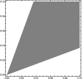

  

  A section along the first diagonal along the line containing the origin O and of the domain ${\|\operatorname {dev}_{3} \log U\|^{2}}<1$. This indicates that, similar to TSTS-M⁺, ellipticity might be controlled by the distortional energy

• In fact it is enough to check where the energy function $F\mapsto e^{\| \operatorname {dev}_{3} \log U\|^{2}}$ looses the ellipticity in all planes λ _i =1, meaning planes π _i containing the point (1,1,1) and orthogonal to the axes Oλ _i , respectively. In view of the symmetry in λ _i , it is enough to see what happens in the plane π ₁:λ ₁=1.

7 Summary and Open Problems

To summarize, in the present paper:

• We have proved that the planar exponentiated Hencky strain energy function

  $$\begin{aligned} F\mapsto W_{{\mathrm{eH}}}(F):=\widehat{W}_{{\mathrm{eH}}}(U):&= \left\{ \begin{array}{l@{\quad }ll} \frac{\mu}{k} e^{k \|\operatorname {dev}_2\log U\|^2}+\frac{\kappa}{2\widehat {k}} e^{\widehat{k} (\operatorname {tr}(\log U))^2}&\text{if}& \det F>0,\\ +\infty& \text{if} &\det F\leq0 \end{array} \right. \end{aligned}$$

  (7.1)

  is rank-one convex for μ>0,κ>0, $k\geq\frac {1}{4}$ and $\widehat{k}\geq\frac{1}{8}$;

• We have shown that the exponentiated volumetric energy function

  $$\begin{aligned} F\mapsto\frac{\kappa}{2\widehat{k}} e^{\widehat{k} (\operatorname {tr}(\log U))^2}, \quad F\in\mathrm{GL}^+(n) \end{aligned}$$

  (7.2)

  is rank-one convex w.r.t. F for the volumetric strain parameter $\widehat{k}\geq\frac{1}{m^{(m+1)}}$. ($m=2: \widehat{k}\geq\frac {1}{8}$, $m=3: \widehat{k}\geq\frac{1}{81}$);

• We have shown that for all distortional strain stiffening parameters k>0 the energy function

  $$\begin{aligned} F\mapsto\frac{\mu}{k} e^{k \|\operatorname {dev}_3\log U\|^2},\quad F \in \mathrm{GL}^+(3) \end{aligned}$$

  (7.3)

  is not rank-one convex;

• Numerical tests suggest that the LH-ellipticity domain of the distortional energy function $F\mapsto\frac{\mu}{k} e^{k \|\operatorname {dev}_{3}\log U\|^{2}}$, F∈GL⁺(3), with $k\geq\frac{3}{16}$ (the necessary condition for separate convexity (SC) of $e^{k \|\operatorname {dev}_{3}\log U\|^{2}}$ in 3D) is an extremely large cone

  $$\begin{aligned} \mathcal{E}(W_{{\mathrm{eH}}},{\mathrm{LH}},U, 27)=\bigl\{ U\in {\mathrm{PSym}}(3) | \|\operatorname {dev}_3\log U\|^2< 27\bigr\} ; \end{aligned}$$

  (7.4)

• We have proved that the energy function

  $$\begin{aligned} F\mapsto\frac{\mu}{k} e^{k \|\log U\|^2},\quad F \in\mathrm {GL}^+(n), \quad n=2,3 \end{aligned}$$

  (7.5)

  is not rank-one convex;

• We have shown that the true-stress-true-strain relation is invertible for the family of energies W _eH;

• The monotonicity of the Cauchy stress tensor, as a function of logV, for our family of exponentiated Hencky energies is true in certain domains of bounded distortions

  $$\begin{aligned} \mathcal{E}\biggl(W_{{\mathrm{eH}}},\text{TSTS-M}^+, \tau _{{\mathrm{eH}}}, \frac{2}{3} {\boldsymbol{\sigma}}_{ \mathbf{y}}^2\biggr):= \biggl\{ \tau\in\mathrm{Sym}(3) | \|\operatorname {dev}_3 \tau\|^2 \leq\frac{2}{3} {\boldsymbol{\sigma}}_{ \mathbf{y}}^2 \biggr\} , \end{aligned}$$

  (7.6)

  superficially similar to the observed ellipticity domains $\mathcal {E}(W_{{\mathrm{eH}}},\text{TSTS-M}^{+}, \tau_{{\mathrm{eH}}},\frac {2}{3} {\boldsymbol{\sigma}}_{ \mathbf{y}}^{2})$;

• For all exponentiated energies KSTS-M⁺, KSTS-I, TSTS-I, TSS-I conditions are satisfied everywhere;

• For n=3 among the family W _eH we have singled out a special ($k=\frac{2}{3} \widehat{k}$) three parameter subset

  $$\begin{aligned} W_{{\mathrm{eH}}}^{\sharp}(\log V)=\frac{1}{2 k} \biggl\{ \frac{E}{1+\nu} e^{k \|\operatorname {dev}_3\log V\|^2}+\frac{E}{2(1-2 \nu )} e^{\frac{2}{3} k (\operatorname {tr}(\log V))^2} \biggr\} \end{aligned}$$

  such that uniaxial tension leads to no lateral contraction if and only if ν=0, as in linear elasticity.

In forthcoming papers [170, 171, 177] our geodesic invariants

$$\begin{aligned} \begin{array}{l@{\qquad }l} \text{``the magnitude-of-dilatation'':} & K_1^2=\bigl|\operatorname {tr}(\log U)\bigr|^2=|\log\det U|^2\\ &\hphantom{K_1^2} =|\log\det V|^2=|\log\det F|^2,\\ \text{``the magnitude-of-distortion'':}& K_2^2=\|\operatorname {dev}_3\log U\|^2=\|\operatorname {dev}_3\log V\|^2, \end{array} \end{aligned}$$

as basic ingredients of idealized isotropic strain energies will be motivated in detail. As already stated in the introduction, it can be shown that [170, 171, 177]

where and $\operatorname {dist}^{2}_{{\mathrm{geod},\mathrm{SL}(n)}}$ are the canonical left invariant geodesic distances on the Lie-group SL(n) and on the group , respectively (see [170, 171, 177]). For this investigation new mathematical tools had to be discovered [132, 177] also having consequences for the classical polar decomposition [118, 119].

Hence, using this terminology, in the present paper we have shown rank-one convexity of

(7.7)

Our W _eH formulation ignores at first sight yield surfaces and other aspects of a theory of plasticity. Yet, our investigation on the ellipticity conditions in 3D suggests a relation between loss of ellipticity conditions and permanent deformations [173].

Let us finish this paper with some conjectures stemming from our unsuccessful attempts in this direction:

Conjecture 7.1

For n=2,3 the energy $F\mapsto\frac{\mu}{k} e^{k \|\operatorname {dev}_{n}\log U\| ^{2}}$, $k>\frac{3}{16}$ is rank-one convex in a set which contains the large cone

$$\begin{aligned} \mathcal{E}(W_{{\mathrm{eH}}},{\mathrm{LH}},U,27)=\bigl\{ U\in {\mathrm{PSym}}(3) | \|\operatorname {dev}_3\log U\|^2< 27\bigr\} . \end{aligned}$$

(7.8)

Moreover, it would be interesting to know the rank-one convex and quasiconvex envelope of the energy $F\mapsto\frac{\mu}{k}e^{k \| \operatorname {dev}_{n}\log U\|^{2}}$, $k>\frac{3}{16}$.

Conjecture 7.2

For n=3 there is no elastic energy expression

$$\begin{aligned} W=W\bigl(K_2^2\bigr)=W\bigl(\|\operatorname {dev}_3\log U \|^2\bigr) \end{aligned}$$

(7.9)

such that $F\mapsto W(\|\operatorname {dev}_{3}\log U\|^{2})$ is Legendre-Hadamard elliptic in GL⁺(3), i.e., over the entire deformation range.

Conjecture 7.3

For n=2,3 there is no elastic energy expression

$$\begin{aligned} W=W\bigl(K_2^2\bigr)=W\bigl(\|\operatorname {dev}_n\log U \|^2\bigr) \end{aligned}$$

(7.10)

such that $F\mapsto W(\|\operatorname {dev}_{n}\log U\|^{2})$ satisfies the TSTS-M ⁺ condition in GL⁺(n), i.e., over the entire deformation range.

A further open problem is to find an energy $F\mapsto W(\|\operatorname {dev}_{3}\log U\|^{2}, [\operatorname {tr}(\log U)]^{2})$ such that the BSS-I condition is satisfied. In a future contribution we will discuss the application of the family W _eH(F) to the description of large strain rubber elasticity for Treloar’s classical data.

Appendix

1.1 A.1 Some Useful Identities

• $\operatorname {tr}(B^{-1}X B)=\operatorname {tr}(X)$ for any invertible matrix B.

• $\operatorname {dev}_{n}(B^{-1}X B)=B^{-1}X B-\frac{1}{n} \operatorname {tr}(B^{-1}X B)=B^{-1}(\operatorname {dev}_{n} X) B$ for any invertible matrix B.

• .

• The norm of the deviator in $\mathbb {R}^{n\times n}$:

  $$\begin{aligned} \left \Vert \operatorname {dev}_n\left ( \begin{array}{c@{\quad}c@{\quad}c@{\quad}c} \xi_1&0&\cdots&0\\ 0&\xi_2&\cdots&0\\ \vdots&\vdots&\ddots&\vdots\\ 0&0&\cdots&\xi_n\\ \end{array} \right ) \right \Vert ^2&=\sum_{i=1}^n \xi_i^2-\frac{1}{n}\Biggl(\sum_{i=1}^n \xi_i\Biggr)^2 =\frac{n-1}{n}\sum _{i=1}^n \xi_i^2- \frac{2}{n}\sum_{i,j=1,i< j}^n \xi_i\xi_j \\ &=\frac{1}{n}\Biggl[(n-1)\sum_{i=1}^n \xi_i^2-2\sum_{i,j=1,i<j}^n \xi_i\xi_j\Biggr] \\ &=\frac{1}{n}\sum_{i,j=1,i<j}^n \bigl( \xi_i^2-2 \xi_i\xi_j+ \xi_j^2\bigr)=\frac{1}{n}\sum _{i,j=1,i<j}^n (\xi_i-\xi_j)^2. \end{aligned}$$

  (A.1)

• From [165, page 200] we have: $\frac{\|X\| ^{p}}{z^{\alpha}}$ is convex in (X,z) if $\frac{\alpha+1}{\alpha}\geq \frac{p}{p-1}\Leftrightarrow p\geq\alpha+1$.

• $\log U=\sum_{i=1}^{n} \log\lambda_{i} N_{i}\otimes N_{i}$, where N _i are the eigenvectors of U and λ _i are the eigenvalues of U.

• , convergent for .

• $\log V=\sum_{i=1}^{n} \log\widehat{\lambda}_{i} \widehat {N}_{i}\otimes\widehat{N}_{i}$, where $\widehat{N}_{i}$ are the eigenvectors of V and $\widehat{\lambda}_{i}$ are the eigenvalues of V.

• , convergent for .

• $$\begin{aligned} \left ( \begin{array}{c@{\quad}c} F_{11} & F_{12} \\ F_{21} & F_{22} \\ \end{array} \right )^{-1}=\frac{1}{F_{11}F_{22}-F_{12}F_{21}}\left ( \begin{array}{c@{\quad}c} F_{22} & -F_{12} \\ -F_{21} & F_{22} \\ \end{array} \right )\quad\Rightarrow\quad\|F^{-1}\|^2 \overset{n=2}{=} \frac{1}{(\det F)^2}\|F\|^2. \end{aligned}$$
• $$\begin{aligned} F=\left ( \begin{array}{c@{\quad}c} F_{11} & F_{12} \\ F_{21} & F_{22} \\ \end{array} \right ),\qquad U^2=F^T F=\left ( \begin{array}{c@{\quad}c} F_{11}^2+F_{21}^2 & F_{11} F_{12}+F_{21} F_{22} \\ F_{11} F_{12}+F_{21} F_{22} & F_{12}^2+F_{22}^2 \\ \end{array} \right ). \end{aligned}$$

  The eigenvalues of U ² are:

  $$\begin{aligned} \mu_1&=\frac{1}{2} \Bigl(F_{11}^2+F_{12}^2+F_{21}^2+F_{22}^2- \sqrt{ \bigl(F_{11}^2+F_{12}^2+F_{21}^2+F_{22}^2 \bigr){}^2-4 (F_{12} F_{21}-F_{11} F_{22} ){}^2} \Bigr) \\ &=\frac{1}{2} \bigl(\|F\|^2-\sqrt{\|F\|^4-4(\det F)^2} \bigr), \\ \mu_2&=\frac{1}{2} \Bigl(F_{11}^2+F_{12}^2+F_{21}^2+F_{22}^2+ \sqrt{ \bigl(F_{11}^2+F_{12}^2+F_{21}^2+F_{22}^2 \bigr){}^2-4 (F_{12} F_{21}-F_{11} F_{22} ){}^2} \Bigr) \\ &=\frac{1}{2} \bigl(\|F\|^2+\sqrt{\|F\|^4-4(\det F)^2} \bigr). \end{aligned}$$

  The principal stretches of F, i.e., the eigenvalues of $U=\sqrt{F^{T} F}$, which are the same as the eigenvalues of $V=\sqrt{F F^{T}}$, are $\lambda_{1}(F)=\sqrt{\mu_{1}}, \lambda_{2}(F)=\sqrt{\mu_{2}}$.

• Taking the pure stretch under shear stress $F_{1}= \bigl( {\scriptsize\begin{matrix} \cosh\frac{t}{2} & \sinh\frac{t}{2} & 0 \cr \sinh\frac{t}{2} & \cosh\frac{t}{2} & 0 \cr 0 & 0 & 1 \end{matrix}} \bigr)$ and the simple glide $F_{2}= \bigl( {\scriptsize\begin{matrix} 1 & t& 0 \cr 0 & 1 & 0 \cr 0 & 0 & 1 \end{matrix}} \bigr)$, the corresponding rates $L_{1}(t)=\frac{{\mathrm{d}}}{{\mathrm{dt}}}F_{1}\cdot F_{1}^{-1}\neq \frac{{\mathrm{d}}}{{\mathrm{dt}}}F_{2}\cdot F_{2}^{-1}=L_{2}(t)$ are different, as is $\log U_{1}(t)\neq \log\sqrt{F_{2}^{T}F_{2}}=\log U_{2}(t)$ and $\frac{{\mathrm {d}}}{{\mathrm{dt}}}\log U_{1}\neq\frac{{\mathrm{d}}}{{\mathrm {dt}}}\log U_{2}(t)$. However, D ₁(t)=sym L ₁(t)=sym L ₂(t)=D ₂(t). This shows that $\frac {{\mathrm{d}}}{{\mathrm{dt}}}\log U(t)=D(t)$ is true only for coaxial families U(t).

1.2 A.2 Vallée’s Formula

Lemma A.1

(Vallée’s formula³² (see also [130, 210, 256, 257]))

Let us consider S∈Sym(3) and let $\varPsi:\mathrm {Sym}(3)\rightarrow \mathbb {R}$ be a differentiable isotropic scalar value function. We define W(S)=Ψ(exp(S)). Then, the following chain rules hold:

$$\begin{aligned} \begin{aligned} &D_S\bigl[\varPsi\bigl(\exp(S)\bigr) \bigr]=\exp(S)\cdot D \varPsi\bigl(\exp(S)\bigr), \qquad D_SW(S)=D \varPsi\bigl(\exp(S)\bigr)\cdot\exp(S), \\ &D_C \varPsi(C)=D W(\log C)\cdot C^{-1},\qquad C\cdot D_C\varPsi(C)=D W(\log C), \end{aligned} \end{aligned}$$

(A.2)

while it is generally not true that D _C [logC].H=〈C ⁻¹,H〉.

Proof

Let us first remark that

(A.3)

Further we consider the Taylor expansion of the function Ψ(exp(S))

$$\begin{aligned} &\varPsi\bigl(\exp(S+H)\bigr) \\ &\quad=\varPsi\bigl(\exp(S)+D\bigl(\exp(S)\bigr). H+\cdots\bigr) \\ &\quad=\varPsi\bigl(\exp(S)\bigr)+\bigl\langle D \varPsi\bigl(\exp (S)\bigr), D\bigl( \exp(S)\bigr). H\bigr\rangle +\cdots \\ &\quad=\varPsi\bigl(\exp(S)\bigr)+\biggl\langle D \varPsi\bigl(\exp (S)\bigr), H+ \frac{1}{2}(S H+H S)\biggr\rangle \\ &\qquad+\biggl\langle D \varPsi\bigl(\exp(S)\bigr),\frac{1}{6}(S S H+S H S+H S S)+\cdots\biggr\rangle +\cdots \\ &\quad=\varPsi\bigl(\exp(S)\bigr)+\bigl\langle D \varPsi\bigl(\exp (S)\bigr), H\bigr\rangle +\frac{1}{2} \bigl\langle D \varPsi\bigl(\exp(S)\bigr),S H+H S\bigr\rangle \\ &\qquad+\frac{1}{6}\bigl\langle D \varPsi\bigl(\exp(S)\bigr),SSH+S H S+H S S\bigr\rangle +\cdots \\ &\quad=\varPsi\bigl(\exp(S)\bigr)+\bigl\langle D \varPsi\bigl(\exp (S)\bigr), H\bigr\rangle +\frac{1}{2} \bigl[\bigl\langle S^T D \varPsi\bigl(\exp(S) \bigr), H\bigr\rangle +\bigl\langle D \varPsi\bigl(\exp(S)\bigr) S^T,H \bigr\rangle \bigr] \\ &\qquad+\frac{1}{6} \bigl[S^T S^T \bigl\langle D \varPsi\bigl(\exp(S)\bigr),H\bigr\rangle +\bigl\langle S^T D \varPsi \bigl( \exp(S)\bigr) S^T,H\bigr\rangle \\ &\qquad+\bigl\langle D \varPsi\bigl(\exp(S)\bigr) S^T S^T,H\bigr\rangle \bigr]+\cdots. \end{aligned}$$

(A.4)

Since S∈Sym(3), it follows

$$\begin{aligned} \varPsi\bigl(\exp(S+H)\bigr)&=\varPsi\bigl(\exp(S)\bigr)+\bigl\langle D \varPsi\bigl( \exp(S)\bigr), H\bigr\rangle \\ &\quad+\frac{1}{2} \bigl[\bigl\langle S D \varPsi\bigl(\exp(S)\bigr), H \bigr\rangle +\bigl\langle D \varPsi\bigl(\exp(S)\bigr) S,H\bigr\rangle \bigr] \\ &\quad+\frac{1}{6} \bigl[S S \bigl\langle D \varPsi\bigl(\exp (S)\bigr),H \bigr\rangle +\bigl\langle S D \varPsi\bigl(\exp(S)\bigr) S,H\bigr\rangle \\ &\qquad+\bigl\langle D \varPsi\bigl(\exp(S)\bigr) S S,H\bigr\rangle \bigr]+\cdots. \end{aligned}$$

(A.5)

On the other hand, since DΨ is a isotropic tensor function and obvious exp(S) is also isotropic, we have that DΨ(exp(S)) is also a isotropic tensor function and therefore it holds

$$\begin{aligned} D \varPsi\bigl(\exp(S)\bigr)\cdot S=S\cdot D \varPsi\bigl(\exp(S)\bigr). \end{aligned}$$

(A.6)

Therefore,

(A.7)

Using again the isotropy of DΨ(exp(S)), we obtain

$$\begin{aligned} \varPsi\bigl(\exp(S+H)\bigr) &=\varPsi\bigl(\exp(S)\bigr)+\bigl\langle \exp(S)\cdot D \varPsi\bigl(\exp(S)\bigr),H\bigr\rangle + \cdots. \end{aligned}$$

(A.8)

We recall that we simultaneously have

$$\begin{aligned} \varPsi\bigl(\exp(S+H)\bigr) &=\varPsi\bigl(\exp(S)\bigr)+\bigl\langle D_S \varPsi\bigl(\exp(S)\bigr),H\bigr\rangle +\cdots, \end{aligned}$$

(A.9)

for all H∈Sym(3). Thus, we deduce

$$\begin{aligned} \begin{aligned} &\bigl\langle D_S\varPsi\bigl(\exp(S)\bigr),H\bigr\rangle =\bigl\langle \exp(S)\cdot D \varPsi\bigl(\exp(S)\bigr),H\bigr\rangle , \\ &\bigl\langle D_SW(S),H\bigr\rangle =\bigl\langle \exp(S)\cdot D \varPsi\bigl(\exp(S)\bigr),H\bigr\rangle . \end{aligned} \end{aligned}$$

(A.10)

Choosing S=logC, the relations (A.2)₃ also results and the proof is complete. □

1.3 A.3 LH-Ellipticity for Functions of the Type F↦h(detF)

We consider a function $h:\mathbb {R}\to \mathbb {R}$ and we analyze when the function F↦h(detF) is LH-elliptic as a function of F, $F\in \mathbb {R}^{3\times3}$. We recall that

$$\begin{aligned} D(\det F).H=\det F\cdot \operatorname {tr}\bigl(H F^{-1}\bigr)=\langle \operatorname {Cof}F,H \rangle. \end{aligned}$$

(A.11)

Using the first Frechét-formal derivative, we compute the derivative

$$\begin{aligned} D\bigl(h(\det F)\bigr).(H,H)=h^{\prime}(\det F)\cdot\langle \operatorname {Cof}F, H \rangle, \end{aligned}$$

(A.12)

and the second derivative will be

$$\begin{aligned} &D^2\bigl(h(\det F)\bigr).(H,H) \\ &\quad=h^{\prime\prime}(\det F)\cdot\langle \operatorname {Cof}F, H\rangle ^2+h^{\prime}( \det F)\bigl\langle D(\operatorname {Cof}F).H, H\bigr\rangle \\ &\quad=h^{\prime\prime}(\det F)\cdot\langle \operatorname {Cof}F, H\rangle ^2+h^{\prime}( \det F) \bigl\{ \bigl\langle \langle \operatorname {Cof}F,H\rangle F^{-T},H\bigr\rangle \\ &\qquad+\det F\bigl\langle -F^{-T}H^T F^{-T},H \bigr\rangle \bigr\} , \\ &\quad=h^{\prime\prime}(\det F)\cdot\langle \operatorname {Cof}F, H\rangle ^2+h^{\prime} (\det F) \det F \bigl\{ \bigl\langle F^{-T},H\bigr\rangle ^2 \\ &\qquad-\bigl\langle F^{-T}H^T F^{-T},H\bigr\rangle \bigr\} . \end{aligned}$$

(A.13)

Hence, for $\xi,\eta\in \mathbb {R}^{3}$ we have

$$\begin{aligned} &D^2\bigl(h(\det F)\bigr).(\xi\otimes\eta,\xi\otimes\eta)) \\ &\quad=h^{\prime\prime}(\det F)\cdot\bigl\langle \operatorname {Cof}F, (\xi \otimes\eta) \bigr\rangle ^2+h^{\prime} (\det F) \det F \bigl\{ \bigl\langle F^{-T},(\xi\otimes\eta)\bigr\rangle ^2 \\ &\qquad-\bigl\langle F^{-T}(\xi\otimes\eta)^T F^{-T},(\xi\otimes\eta)\bigr\rangle \bigr\} . \end{aligned}$$

(A.14)

On the other hand

This leads to the surprising simplification

$$\begin{aligned} D^2\bigl(h(\det F)\bigr).&(\xi\otimes\eta,\xi\otimes \eta)=h^{\prime\prime}(\det F)\cdot\bigl\langle \operatorname {Cof}F, (\xi \otimes\eta)\bigr\rangle ^2. \end{aligned}$$

(A.15)

In conclusion, F↦h(detF) is LH-elliptic if and only if t↦h(t) is convex since $\langle \operatorname {Cof}F, (\xi\otimes\eta )\rangle^{2}$ is positive.

From [55, page 213] we know more:

Proposition A.2

Let $W:\mathbb{R}^{n\times n}\rightarrow\mathbb{R}$ be quasiaffine but not identically constant and $h:\mathbb{R}\rightarrow\mathbb{R}$ be such that W(F)=h(detF). Then

$$\begin{aligned} W \textit{polyconvex}\quad\Leftrightarrow\quad W \textit {quasiconvex}\quad \Leftrightarrow\quad W \textit{rank one convex}\quad\Leftrightarrow \quad h\ \textit{convex}. \end{aligned}$$

(A.16)

1.4 A.4 Convexity for Functions of the Type t↦ξ((logt)²)

We consider a generic function $\xi:\mathbb {R}_{+}\to \mathbb {R}_{+}$ and we find a characterization of the convexity for the function t↦ξ((logt)²). In the following let ζ denote the function $\zeta:\mathbb {R}_{+}\to \mathbb {R}_{+}$ , ζ(t)=(logt)². We deduce

$$\begin{aligned} \begin{aligned} \frac{\mathrm{d}}{\mathrm{dt}}{\xi}\bigl((\log t)^2\bigr)&= \xi^{\prime}\bigl((\log t)^2\bigr) 2 \frac{1}{t} \log t, \\ \frac{{\mathrm{d}}^2 }{{\mathrm{dt}}^2}\xi\bigl((\log t)^2\bigr)&=2\frac{\mathrm{d}}{\mathrm{dt}} \biggl(\xi^{\prime}\bigl((\log t)^2\bigr) 2 \frac{1}{t} \log t \biggr) \\ &=4 \xi^{\prime\prime}\bigl((\log t)^2\bigr) \frac{1}{t^2} ( \log t)^2-2 \xi^{\prime}\bigl((\log t)^2\bigr) \frac{1}{t^2} \log t+2 \xi^{\prime}\bigl((\log t)^2\bigr) \frac{1}{t^2} \\ &=2\frac{1}{t^2} \bigl[{2} \xi^{\prime\prime}\bigl((\log t)^2 \bigr) (\log t)^2 +\xi^{\prime}\bigl((\log t)^2 \bigr) (1- \log t) \bigr], \end{aligned} \end{aligned}$$

(A.17)

where $\xi^{\prime}=\frac{d \xi}{d\zeta}$. Hence, the function t↦ξ((logt)²) is

• convex on [1,∞) as a function of t if and only if $2\frac{d^{2}\xi(\zeta)}{d\zeta^{2}} \zeta+ {\frac{d\xi(\zeta )}{d\zeta} (}1- \sqrt{\zeta})\geq 0$, for all $\zeta\in \mathbb {R}_{+}$.

• convex on (0,1) as a function of t if and only if $2\frac{d^{2}\xi(\zeta)}{d\zeta^{2}} \zeta+ {\frac{d\xi(\zeta )}{d\zeta}(1}+ \sqrt{\zeta})\geq 0$, for all $\zeta\in \mathbb {R}_{+}$.

1.5 A.5 Connecting $\operatorname {dev}_{3}\log U$ with $\operatorname {dev}_{2}\log U$

For U ^♯∈GL(2), we define the lifted quantity

$$\begin{aligned} U=\left ( \begin{array}{c@{\quad}c@{\quad}c} &U^\sharp& 0\\ & & 0\\ 0&0&(\det U^\sharp)^{1/2} \end{array} \right )\in\mathrm{GL}(3). \end{aligned}$$

(A.18)

We remark that

$$\begin{aligned} \det \left ( \begin{array}{c@{\quad}c@{\quad}c} &U^\sharp& 0\\ & & 0\\ 0&0&(\det U^\sharp)^{1/2} \end{array} \right )=\det U^\sharp\bigl(\det U^\sharp\bigr)^{1/2}=\bigl(\det U^\sharp \bigr)^{3/2}, \end{aligned}$$

(A.19)

which implies (detU)^1/3=[detU ^♯(detU ^♯)^1/2]^1/3=[(detU ^♯)^3/2]^1/3=(detU ^♯)^1/2. Moreover, we obtain

$$\begin{aligned} \operatorname {dev}_3\log U&=\log\frac{U}{\det U^{1/3}}=\log\frac{U}{(\det U^\sharp)^{1/2}}=\log \left ( \begin{array}{c@{\quad}c@{\quad}c} & \frac{U^\sharp}{(\det U^\sharp)^{1/2}}& 0\\ & & 0\\ 0&0&1 \end{array} \right ) \\ &=\left ( \begin{array}{c@{\quad}c@{\quad}c} & \log\frac{U^\sharp}{(\det U^\sharp)^{1/2}}& 0\\ & & 0\\ 0&0&0 \end{array} \right )=\left ( \begin{array}{c@{\quad}c@{\quad}c} &\operatorname {dev}_2 \log U^\sharp& 0\\ & & 0\\ 0&0&0 \end{array} \right ). \end{aligned}$$

(A.20)

In general, for $A^{\sharp}\in \mathbb {R}^{2\times2}$ and $\alpha\in \mathbb {R}$ we have

$$\begin{aligned} \left\|\operatorname {dev}_3\left ( \begin{array}{c@{\quad}c@{\quad}c} &A^\sharp& 0\\ & & 0\\ 0&0&\alpha \end{array} \right )\right\|^2&=\left\| \left ( \begin{array}{c@{\quad}c@{\quad}c} &A^\sharp& 0\\ & & 0\\ 0&0&\alpha \end{array} \right )\right\|^2-\frac{1}{3} [\operatorname {tr}\left[ \left ( \begin{array}{c@{\quad}c@{\quad}c} &A^\sharp& 0\\ & & 0\\ 0&0&\alpha \end{array} \right )\right]^2 \\ &=\bigl\| A^\sharp\bigr\| ^2+\alpha^2-\frac{1}{3} \bigl[\operatorname {tr}\bigl(A^\sharp\bigr)+\alpha\bigr]^2 \\ &=\bigl\| A^\sharp\bigr\| ^2-\frac{1}{3} \bigl[\operatorname {tr}\bigl(A^\sharp\bigr)\bigr]^2-\frac{2}{3}\alpha \operatorname {tr}\bigl(A^\sharp\bigr) -\frac{1}{3} \alpha^2+ \alpha^2 \\ &=\bigl\| \operatorname {dev}_2 A^\sharp\bigr\| ^2-\frac{2}{3} \alpha \operatorname {tr}\bigl(A^\sharp\bigr) +\frac{2}{3} \alpha^2. \end{aligned}$$

(A.21)

Thus

$$\begin{aligned} \left\|\operatorname {dev}_3\left ( \begin{array}{c@{\quad}c@{\quad}c} &A^\sharp& 0\\ & & 0\\ 0&0&\alpha \end{array} \right )\right\|^2&=\bigl\| \operatorname {dev}_2 A^\sharp\bigr\| ^2 \end{aligned}$$

(A.22)

if and only if α=0 or $\alpha=\operatorname {tr}(A^{\sharp})$. Hence, we deduce ${\|\operatorname {dev}_{3}\log U\|^{2}}={\|\operatorname {dev}_{2}\log U^{\sharp}\|^{2}}$, for U of the form (A.18). Since U ^♯∈PSym(2), we can assume that $U^{\sharp}= \bigl({\scriptsize\begin{matrix}\lambda_{1}&0\cr 0&\lambda_{2}\end{matrix}} \bigr)$, $\lambda_{1},\lambda_{2}\in \mathbb {R}_{+}$. Then, the lifted quantity U lies in $\operatorname {PSym}(3)$ and $U = \bigl({\scriptsize\begin{matrix}\lambda_{1}&0&0\cr 0&\lambda_{2}&0\cr 0&0&(\lambda_{1} \lambda_{2})^{1/2}\end{matrix}} \bigr)$.

The next problem is if for a given deformation $\varphi^{\sharp}=(\varphi_{1}^{\sharp}, \varphi_{2}^{\sharp}):\mathbb {R}^{2}\rightarrow \mathbb {R}^{2}$ such that $U^{\sharp}=\sqrt{(\nabla\varphi^{\sharp})^{T} \nabla\varphi^{\sharp}}$ we can construct an ansatz $\varphi:\mathbb {R}^{3}\rightarrow \mathbb {R}^{3}$ such that $U=\sqrt{\nabla\varphi^{T} \nabla\varphi}$, where U is the lifted quantity associated to U ^♯. For this it is necessary to have φ=(φ ₁(x ₁,x ₂),φ ₂(x ₁,x ₂),x ₃ α(x ₁,x ₂)) and $\alpha_{,x_{1}}=0, \alpha_{,x_{2}}=0$. Checking the compatibility equation we see that this is possible if and only if $\det\nabla \varphi^{\sharp}=K=\mathit{const.}$, which implies $\varphi_{3,x_{3}}=K$. In the incompressible case det∇φ=1, an appropriate ansatz is therefore

$$\begin{aligned} \varphi(x_1,x_2,x_3)=\bigl( \varphi_1^\sharp(x_1,x_2), \varphi_2^\sharp(x_1,x_2),x_3 \bigr), \end{aligned}$$

(A.23)

since

$$\begin{aligned} U^2&={\nabla\varphi^T \nabla\varphi}= \left ( \begin{array}{c@{\quad}c@{\quad}c}&(\nabla\varphi^\sharp)^T \nabla \varphi^\sharp&0\\ &&0\\ 0&0&1 \end{array} \right )=\left ( \begin{array}{c@{\quad}c@{\quad}c}&(\nabla\varphi^\sharp)^T \nabla \varphi^\sharp&0\\ &&0\\ 0&0&\det[(\nabla\varphi^\sharp)^T \nabla\varphi^\sharp] \end{array} \right ) \\ &=\left ( \begin{array}{c@{\quad}c@{\quad}c}&(U^\sharp)^2&0\\ &&0\\ 0&0&(\det[(U^\sharp)^{1/2}])^2 \end{array} \right )=\left ( \begin{array}{c@{\quad}c@{\quad}c}&U^\sharp&0\\ &&0\\ 0&0&(\det U^\sharp)^{1/2} \end{array} \right )^2, \end{aligned}$$

(A.24)

with detU ^♯=1.