A novel deep reinforcement learning scheme for task scheduling in cloud computing

Abstract

Recently, the demand of cloud computing systems has increased drastically due to their significant use in various real-time online and offline applications. Moreover, it is widely being adopted from research, academia and industrial field as a main solution for computation and storage platform. Due to increased workload and big-data, the cloud servers receive huge amount of data storage and computation request which need to be processed through cloud modules by mapping the tasks to available virtual machines. The cloud computing models consume huge amount of energy and resources to complete these tasks. Thus, the energy aware and efficient task scheduling approach need to be developed to mitigate these issues. Several techniques have been introduced for task scheduling, where most of the techniques are based on the heuristic algorithms, where the scheduling problem is considered as NP-hard problem and obtain near optimal solution. But handling the different size of tasks and achieving near optimal solution for varied number of VMs according to the task configuration remains a challenging task. To overcome these issues, we present a machine learning based technique and adopted deep reinforcement learning approach. In the proposed approach, we present a novel policy to maximize the reward for task scheduling actions. An extensive comparative analysis is also presented, which shows that the proposed approach achieves better performance, when compared with existing techniques in terms of makespan, throughput, resource utilization and energy consumption.

1 Introduction

During the last decade, we have noticed tremendous growth in technological advancements. These technical growths raised the demand for high-performing computing (HPC) systems to accomplish the tasks. Nowadays, cloud computing has emerged as a promising solution to facilitate, efficient resources for highly complex tasks [1]. Generally, cloud computing is known as a distributed computing system that consists of a collection of interconnected and virtualized computers that are provisioned dynamically [2]. The newly developed cloud computing (CC) techniques exploits several advantages over traditional high performance computing systems such as: (a) Cloud Computing (CC) techniques facilitate the on demand resources according to the user request and task requirement, (b) It reduces the cost of hardware expenditure because it has shared resources which can be used based on the “pay-per-use” model, (c) It ensures the user satisfaction because it works under the conditions of service level agreement (SLA) which is a negotiation process between user and service providers and (d) It uses the virtualization process to create the virtual machine which improves the resource utilization [3]. Generally, the cloud computing consists of three service modules such as infrastructure as service (IaaS) that includes servers, virtual machines, and storage etc., Platform as a service (PaaS) that consists database, web server, execution runtime and development tools etc., and Software as a service (SaaS) that includes virtual desktops, emails and communication setups. Figure 1 illustrates the basic architecture of cloud computing.

Fig. 1

Cloud architecture

The cloud computing techniques are widely adopted by various organizations and real-time applications due to numerous applications and significant computing performance. Moreover, these techniques play a significant role in information and communication technology (ICT) and academic research. Moreover, cloud computing techniques encompasses sundry functionalities and services such as advanced security, efficient distribution of large data in the geographical region, virtualization, resilient computing, web infrastructure, and various web-related applications. The cloud computing technology offers several services such as data processing, storing, computing resources, virtual desktops, virtual services, web-based deployment platforms, web services, and databases. It uses the “pay-as-you-go” model offered by cloud service providers for specific applications. The cloud computing offers several benefits such as energy efficiency, cost-saving, flexibility, faster implementation, and scalability [4,5,6].

In this field of computing applications, several techniques are being presented based on technological advancements such as distributed computing, parallel computing, grid computing, cluster computing, mobile computing, fog computing, and cloud computing. Due to the increment in technology such as IoT, sensor networks, and mobile applications [7], a huge amount of data is generated and stored on cloud servers. This increased data requires huge resources and consumes excessive energy while processing these data. Thus, cloud computing has emerged as a promising solution to deal with these issues and offers a virtualization process by creating virtual computing machines at cloud data centers. These characteristics of cloud computing (CC) considered as a big breakthrough in green computing. However, minimizing energy consumption and efficient resource allocation still remains a challenging task [8,9,10].

Currently, the green computing has become one of the hot research topics in high performance computing systems. During the last decade, the internet-based services has surged up where cloud computing based systems are considered as the main cause of increased energy consumption in information and communication technology (ICT) sector. Recently, a study presented in [11] reported that the energy consumption by cloud data center is increasing by 15% annually and energy consumption cost make up about 42% of the total cost of operating of data centers. A study presented in [12] reported that around 6000 data centers are present in USA whose approximated energy consumption was 61 billion kilowatt hours (kWh). In [13], authors discussed that energy consumption rate between 2005 and 2010 was growing at the rate of 24%. It was also reported that data center in US consumed 70 billion kWh power in 2014 which was the 1.8% of the total power consumption.

Thus, minimizing the energy consumption has become an important research topic to improve the green computing systems. Several techniques have been presented to minimize the energy consumption such as load balancing [14, 15], task scheduling [16, 17], virtual machine scheduling [18], VM migration and allocation [19]. Task scheduling is considered as promising technique to minimize the energy consumption which uses efficient resource allocation according to the incoming tasks. Efficient resource allocation for incoming task is a challenging issue because it has a significant impact on the entire system. Generally, the task scheduling techniques distribute the tasks over available resources based on their goals such as load balancing, increasing the resource utilization, reducing the waiting time and system throughput. These tasks can be independent where tasks can be scheduled in any sequence or dependent where the upcoming tasks can only be scheduled after completing the ongoing dependent tasks. The main aim of any novel scheduling algorithm is to balance different types of conflicting parameters simultaneously, such as allocating better resources and maintaining the fair execution time. Several algorithms have been presented which are based on the meta-heuristic optimization schemes such as particle swarm optimization (PSO), genetic algorithm (GA), ant colony optimization, and many more [20]. Similarly, machine learning based schemes are adopted for this purpose such as Q-learning with earliest finish time [21], neural network based approach [22], combination of deep learning and reinforcement learning [23], hybrid particle swarm optimization and fuzzy theory [24], and neural network with evolutionary computation [25] etc. Most of the existing schemes achieve desired performance for a certain limit of tasks and also performs well with the homogenous tasks. As the number of tasks increase, the convergence performance is affected which leads to increase the execution time. In this work, we introduce a reinforcement learning based approach which adapts the environment and updates its working procedure based on the reward and punish mechanism. Moreover, the reinforcement learning learns from the complex environment and makes the decision. This automated adaptive learning helps to minimize the complexity to process the task when compared with the traditional algorithms. Thus, the convergence and the optimization function problem can be solved. Moreover, it focusses on improving the performance of the overall system by considering CPU, RAM, Bandwidth and resource parameters which improve the efficient resource utilization.

1.1 Motivation

Load balancing is a promising technique which helps to distribute the workload evenly among the available virtual machines and computing resources. Its main aim is to facilitate continuous support to the cloud systems by efficient utilization. Moreover, load balancing is the promising technique which minimizes response time for tasks and improves the resource utilization performance. Load balancing also strives to offer scalability and flexibility for applications that may grow in size in the future and demand additional resources, as well as to prioritize operations that require immediate execution above others. Load balancing's other goals include lowering energy usage, minimizing bottlenecks, bandwidth utilization, and meeting QoS criteria for better load balancing. Workload mapping and load balancing approaches that account various metrics are required. However, the current researches need to be improved by developing the fast and responsive scheduling process to accomplish the task requirement. Due to several challenges present in the existing techniques of task scheduling in cloud computing, we focused on the development of a novel scheme for energy efficient task scheduling. The main aim of the proposed approach is to allocate resources efficiently, on time task completion, task scheduling and minimizing the energy consumption.

1.2 Work contribution

In this work, first of all, we present a system model where we describe the architecture of cloud computing, which includes user, cloud broker, VM allocator, VM provisioner, VM scheduler and processing elements. In the next step, we present the problem formulation for task scheduling and minimizing the energy consumption. We define the task model and components of task scheduling. In order to achieve the objective of scheduling and minimizing the energy consumption, we present a deep reinforcement learning model. Finally, a comparative analysis is presented to describe the robustness of the proposed approach.

The rest of the article is arranged in four sections, where Sect. 2 presents a brief description about existing techniques of task scheduling, Sect. 3 presents proposed deep reinforcement learning based model for task scheduling, Sect. 4 presents the comparative analysis based on the obtained performance using proposed approach and finally, Sect. 5 presents the concluding remarks about this approach.

2 Literature survey

This section presents the literature review study about existing techniques of task scheduling and resource allocation in cloud computing. Currently, the energy consumption in cloud data centers has increased drastically. Thus, several researches have been presented to diminish the energy consumption. Most of the traditional techniques are not suitable for the dynamic loads, thus iterative optimization schemes are also widely adopted. Pradeep et al. [1] reported that the efficient task scheduling can be obtained by jointly optimizing the cost, makespan and resource allocation. Based on this, authors presented a hybrid scheduling approach which is a combination of cuckoo search and harmony search algorithm. However, the overall performance of these systems can be improved by optimizing the number of parameters, thus a multi-objective optimization function is presented which considers cost, energy, memory, credit and penalty as the function parameters.

Ebadifard et al. [2] discussed that dynamic task scheduling is a nondeterministic polynomial time (NP) hard problem which can be solved by optimization schemes. Thus, authors developed a PSO based scheduling which considers the tasks as non-preemptive and independent. This approach, focus on the load balancing, where it formulates the resource vector by considering CPU, storage, RAM and bandwidth, whereas several traditional techniques only consider the CPU based resources. This fitness function is designed based on makespan and average utilization. Similarly, Chhabra et al. [6] also considered the task scheduling problem as NP-hard problem and suggested that it can be tackled by meta-heuristic approaches. Thus, authors adopted cuckoo search optimization scheme, but it is identified that the tradition cuckoo-search approach suffer from inaccurate local search, lack of diversity solution and slow convergence problem. These issues cause complexity in load balancing scenarios. To overcome these issues, authors developed a combined approach which uses opposition based learning, cuckoo-search, and differential evolution algorithm to optimize the energy and makespan of incoming loads. The opposition based learning (OBL) generates the optimal initial population. Then, an adaptive mechanism is used to switch between cuckoo-search (CS) and differential evolution (DE) approaches. In [24] Mansouri et al. presented a hybrid approach which uses a combination of modified particle swarm optimization and fuzzy logic theory. In first phase, a new method is presented to update the velocity and roulette wheel selection is used to improve the global search capability. In the next phase, it applies crossover and mutation operators to deal with the local optima issue of PSO. Finally, a fuzzy logic based inference system is applied to compute the overall fitness of the system. In order to compute the fitness function, authors used task length, CPU speed, RAM, and execution time. The designed fitness function minimizes the executing time and resource wastage. Sulaiman et al. [26] focused on developing the energy efficient and low complexity scheduling approach. In order to achieve this objective, authors developed hybrid heuristic and genetic algorithm based approach. This approach improves the quality of initial population generated by the genetic algorithm.

On the other hand, the machine learning based approaches are also widely adopted in this field. Tong et al. [21] presented a combined approach which uses Q-learning and heterogeneous earliest finish time (HEFT) approach. The Q-learning approach uses a reward mechanism which is improved by incorporating the upward rank parameter from HEFT approach. Moreover, the self-learning process of Q-learning helps to update the Q-table efficiently. The complete process is divided into two phases, where first of all Q-learning is applied, which sorts the tasks to generate the optimal task order for processing and later earliest finish time strategy is applied to allocate the tasks to most suitable virtual machine (VM).

Sharma et al. [22] focused on energy efficient task scheduling using machine learning techniques. In this work, authors presented a neural network based approach to achieve the reduced makespan, minimized energy consumption, computation overhead and number of active racks, which can improve the overall performance of the datacenters. This is a supervised learning scheme which considers the historical task data and predicts the most suitable available resources for numerous tasks.

Currently, deep learning techniques have gained huge attention from research community, industries and academic field because of their significant nature of pattern learning. Based on this assumption, Rjoub et al. [23] adopted deep learning scheme for cloud computing scenario and combined it with reinforcement learning scheme to perform the load balancing. Specifically, this work presents four different schemes which are reinforcement learning (RL), deep Q networks, recurrent neural network long short-term memory (RNN-LSTM), and deep reinforcement learning combined with LSTM (DRL-LSTM).

Machine learning techniques are categorized as supervised and unsupervised learning. The supervised learning schemes classify the data based on the pre-labelled dataset, which is trained based on the historical features whereas unsupervised schemes generate the groups of similar data. Based on this concept, Negi et al. [25] presented a hybrid approach which uses artificial neural network (ANN) as supervised learning, clustering as unsupervised learning and type 2 fuzzy logic as soft computing technique for load balancing. The complete approach is divided into two phases, where first of all it includes ANN based load balancing which clusters the virtual machines into under loaded and overloaded VMs with the help of Bayesian optimization and improved K-means approach. In next phase, the multi-objective TOPSIS-PSO algorithm is presented to perform the load balancing.

Ding et al. [30] authors developed a Q-learning based energy efficient task schedule for cloud computing module, this scheme is carried out into two states: in first phase, a centralized dispatcher is used for M/M/S queuing model which helps to assign the incoming user requests to suitable server on cloud. In next phase, a Q-learning based scheduler is applied to prioritize the tasks by continuously updating the policy to assign tasks to virtual machines.

Hoseiny et al. [31] introduced internet based distributed computing called as volunteer computing which is based on the resource sharing paradigm. The volunteers with extra resources share the available extra resources to handle the large-scale tasks. However, the power consumption, computation cost and latency are the well-known issues in distributed computing systems. To overcome these issues, authors considered this as NP-hard task scheduling problem and developed, two mechanisms namely Min-CCV (computation-communication-violation) and Min-V (Violation).

Abualigah et al. [32] considered task scheduling as a critical challenge in cloud computing. To achieve the minimum makespan and maximum resource utilization, authors developed an optimization scheme with elite based differential evolution approach called as MALO (Multi-objective Antlion optimizer). This technique is able to tackle the multi-objective task scheduling problem. The MALO simultaneously minimize the makespan and improves the resource utilization.

Hoseiny et al. [33] developed a novel scheduling algorithm in fog-cloud computing named as PGA (Priority Genetic Algorithm). The main aim of the PGA approach is to improve the overall performance of the system through scheduling, by considering computation time, energy requirement and task deadlines. In order to achieve this, genetic algorithm based optimization scheme is presented to prioritize the tasks which can be assigned further for processing according to VMs capacity.

This section described several related works to improve the energy performance of cloud computing systems with the help of energy aware task scheduling, resource allocation, VMs scheduling and many more. Table 1 shows the comparative analysis of these techniques. The complete study focused on the optimization and machine learning process to perform the task scheduling. The optimization techniques suffer from the convergence issues and machine learning based methods suffer from the appropriate training, data labeling and clustering errors etc.

Table 1 Comparative analysis of existing techniques

3 Proposed model

This section presents the proposed solution for energy aware task scheduling based on self-learning approach for heterogeneous cloud computing environment. In these scenarios, the cloud data centers receive numerous tasks where identifying the correct execution order and then allocating the task to the best suitable virtual machine (VM) plays an important role. This can be obtained by a decision making strategy. Moreover, the tasks are heterogeneous and loaded randomly to the servers, thus a self-learning mechanism can be a promising solution for these scenarios. Based on these assumptions, we present an energy aware task scheduling approach based on reinforcement learning.

3.1 System model

We consider a cloud computing based task scheduling framework as depicted in below given Fig. 2. As mentioned before, the cloud data centers receive computationally intensive tasks which cannot be performed at local devices thus, the cloud centers create virtual machines with different configuration and tasks are allocated to these machines. In this work, we mainly focus on the task scheduling and its resources. We assume that the cloud datacenter has several virtual machines and a task scheduler which has complete information about incoming tasks and capacity details of other virtual machines which includes task size, computation speed in million instructions per second (MIPS), expected time to complete the tasks and waiting time for the task in the queue. The scheduler observes this information and generates the scheduling decision which includes where and when to schedule the task based on their start time, end time and bandwidth requirement. Below given Fig. 2 depicts the working process of a cloud computing system. For simplicity, we consider that real-time tasks are characterized by start time ${s}_{i}$, deadline ${d}_{i}$ and task length ${l}_{i}$.

Fig. 2

Schematic of cloud computing model

In the first phase, the cloud user submits real-time tasks at time ${s}_{i}$ to a cloud computing (CC) environment. After submission of real-time tasks, the user has an assurance that the outcome of these tasks will be received by the deadline ${d}_{i}$. Similarly, the cloud computing (CC) environment is further divided into multiple VMs which are characterized by their processing capacities. The VM unit contains a processing element (PE) which require power to accomplish the assigned tasks. Further, VM allocator search for the host where the VM can find its required resources to complete the task. The VM allocator also considers that the total maximum MIPS of all VMs allocated to host should not exceed the maximum power of the host. Further, these hosts use VM provisioner to map the PEs of a host selected by VM allocator. Finally, the VM schedulers facilitate the processing power of PEs to each VM based on their requirement to complete the task.

The main aim of our work is to increase the task completion rate in the given time duration without wasting the resources. Thus, for a known resource provisioning $\delta$ and a scheduling plan $\beta$, the first objective function is defined as maximizing [34] the successful task completion rate (STCR) given as:

$$STCR=\underset{{T}_{i}\in T}{\mathrm{max}}\left\{{t}_{i}^{F}\left(\delta ,\beta \right)\right\}$$

(1)

where ${t}_{i}^{F}$ denotes the task completion time of task $i$ which is allocated to ${VM}_{j}$.

Further, we consider the power consumption issue by PEs to complete the task. Let us consider that static and dynamic power consumption of host is given as:

$$P={P}_{static }+{P}_{dynamic }$$

(2)

The static power denotes the power consumed by the host when it is in idle mode and it remains unchanged when the host is turned on. Thus, the static power is denoted as:

$${P}_{static }=\alpha {P}_{max}$$

(3)

where $\alpha$ denotes the ratio of static power and maximum power of host and ${P}_{max}$ is the maximum power consumed by the host. Similarly, the dynamic power consumption can be expressed as [35]:

$${P}_{dynamic }\left(u\right)=\left({P}_{max }-{P}_{static}\right){u}^{2}$$

(4)

where $u$ denotes the utilization of a host at a specific time.

The computing power of a host at a given time is related to its efficiency. Thus, the energy required by host to deliver maximum efficiency is denoted as:

$${E}_{max}={\int }_{0}^{{t}_{max}}{P}_{max}dx={P}_{max}{t}_{max}$$

(5)

where ${t}_{max}$ is the time, where the host operates at maximum power to complete the certain types of instructions. Let us consider the power used by the system is $P\left(u\right)$, then the energy consumption can be expressed as:

$$E={\int }_{0}^{\frac{{t}_{max}}{u}}P\left(u\right)dt$$

(6)

Thus, the overall energy consumption of host to complete the tasks can be expressed as:

$$E=\left[\alpha +\left(1-\alpha \right){u}^{2}\right]\frac{{P}_{max}{t}_{max}}{u}$$

(7)

Thus, minimizing the power consumption becomes our second objective. The overall objectives of this work are:

$$\begin{aligned} & \left\{ {Min\sum\limits_{{j = 1}}^{J} {\sum\limits_{{n = 1}}^{N} {\sum\limits_{{m = 1}}^{M} {\left[ {E\left( {{\mathbb{T}}_{n}^{j} \left( j \right)} \right)} \right]} } } } \right. \\ & s.t.\sum\limits_{{j = 1}}^{J} {\sum\limits_{{n = 1}}^{N} {\left| {{\mathbb{T}}_{n}^{j} \left( m \right)} \right|} } \le m_{{slot}} \\ & s.t.T_{w} \times T_{{idle}} = 0 \\ \end{aligned}$$

(8)

According to this equation, the energy consumption should be minimized, moreover, the waiting time ${T}_{w}$ and idle slots ${T}_{idle}$ also should be avoided which improves the efficiency of the overall resource utilization.

3.2 Task and scheduling model

In this section, we present the heterogeneous incoming task model and their scheduling process. In this model we assume that heterogeneous and computationally intensive tasks are arriving at the cloud server which are classified into $K$ categories as $J=\left\{{j}_{1},{j}_{2},..,{j}_{K}\right\}$. The tasks which belong to same category have the same characteristics such as million instructions (MI), task start time, finish time and bandwidth. The task $i$ which belong to $K$ category can be represented as:

$${j}_{i,k}=\langle {a}_{i}.{z}_{i},{l}_{i},{d}_{i}\rangle$$

(9)

where ${a}_{i}$ denotes the task arriving time, ${l}_{i}$ is the size of task, ${d}_{i}$ is the expected delay of task and ${z}_{i}$ is the bandwidth.

The cloud computing servers are configured with several heterogeneous virtual machines as $V=\left\{{v}_{1},{v}_{2},\dots ,{v}_{M}\right\}$. Task scheduler plays important role by deciding the task scheduling order and selection of most suitable VM. Generally, these types of mechanism follow a queuing process, where before scheduling the task, it is placed in the waiting slot which is later vacated after successful scheduling of task and another task is placed in the empty waiting queue. The response time of tasks after scheduling is obtained by including the waiting time and execution time. Thus, the expected time of scheduling task $i$ in ${j}^{th}$ VM can be computed as:

$${e}_{i,j}=\frac{{l}_{i}}{{v}_{j}}$$

(10)

Let us consider that task start time ${s}_{i,j}$ and finish time ${f}_{i,j}$ of task $i$ on ${j}^{th}$ VM. The starting time of other incoming tasks depends on the finish time of previously scheduled task. Thus, the starting time for incoming tasks can be denoted as ${s}_{i,j}=\mathrm{max}\left\{{f}_{i,j},{a}_{i}\right\}$ and task finish time can be expressed as ${f}_{i,j}={s}_{i,j}+{e}_{i,j}$, where ${e}_{i,j}$ represents the time required by VM to process the task. Similarly, the response time for task $i$ can be computed with the help of waiting time and execution time. The response time can be expressed as:

$${t}_{i,j}={w}_{i,j}+{e}_{i,j}$$

(11)

where ${w}_{i,j}$, denotes the waiting time. If the task which is in queue is processed immediately then there is no waiting period, otherwise the gap between starting time and arriving time can be given as ${w}_{i,j}={s}_{i,j}-{a}_{i}$. Based on these parameters, the successful task completion rate (STCR) can be computed as:

$${g}_{i,j}=\frac{{\mathcal{l}}_{i}}{{t}_{i,j}}$$

(12)

where $\mathcal{l}$ denotes the expected latency value and $g$ is the successful task completion rate. To accomplish this, we present reinforcement learning based approach which helps to improve the performance of task scheduling mechanism.

3.3 Proposed scheduling model using deep reinforcement learning

Generally, the main concept of reinforcement learning is to design an agent based system, which can adapt the change in the environment and behave in that environment accordingly. In this work, we apply Q-learning based approach to optimize the scheduling scheme based on the decisions and evaluating the feedback from cloud environment. Let us consider that total $T$ tasks as $T=\left\{{t}_{1},{t}_{2},{t}_{3},\dots ,{t}_{n}\right]$ are submitted to cloud sever which contains total $V$ virtual machines as $V=\left\{{v}_{1},{v}_{2},\dots ,{v}_{m}\right\}$. This learning scheme works in three phases by computing state space, action space and rewards. Let us consider that ${s}_{t}$ denotes the task scheduler state in state space $S$ at time $t$, and ${a}_{t}$ denotes the action in the action space $A$ at time $t$ with probability $P\left({s}_{1}|s,\mathcal{a}\right)=P\left[{s}_{t+1}={s}_{1}|{s}_{t}=s,{\mathcal{a}}_{t}=\mathcal{a}\right]$, where $\sum_{{s}_{1}\in S} P\left({s}_{1}|s,\mathcal{a}\right)=1$. In this model, we consider a cloud scheduler policy as $\pi \left(\mathcal{a}|s\right)$, which is used for mapping the states to actions. Table 2 shows the notations used in this work.

Table 2 Main notations used in this work

The reward of the action ${a}_{t}$ in state ${s}_{t}$ is denoted by ${r}_{t}$. The main aim of this scheduler is to obtain the optimal scheduling policy to minimize the cost for all available VMs and tasks. The states, actions and rewards of the reinforcement learning can be considered as follows:

• State space: In our model, at each time $t$ the state space ${s}_{t}$ represents the present scheduling of the tasks on the VMs, where each VM is characterized based on its available resources such as CPU, RAM, bandwidth and storage space.

• Action space: In current state space, the action state ${a}_{t}$ denotes the scheduling action at time $t$ for all the tasks scheduled on the VMs. Specifically, for each task, this action is denoted as 0 or 1, which is a decision process, represents whether the task is scheduled to VM or not.

• Reward: The reward function denotes the efficiency of the task scheduling process. Let us assume that, task ${t}_{i}$ is assigned to the VM ${v}_{j}$ then, we define the execution cost as ${\zeta }_{i,j}$ which is considered as an immediate reward for this action. Similarly, the overall reward for all the scheduling actions can be obtained by adding the execution cost for each task. The reward for individual task is defined in terms of CPU, bandwidth, RAM and storage as follows:

  $${\zeta }_{i,j}=\left({\psi }_{i,j}+ {w}_{i,j}\right)\times {\mathbb{P}}_{j}$$

  (13)

where ${w}_{i,j}$ denotes the waiting time for task ${t}_{i}$ to be assigned to its corresponding VM, ${\mathbb{P}}_{j}$ denotes the price for virtual machine, and ${\psi }_{i,j}$ is the execution time of task on assigned VM. In this approach, we focus on optimizing the scheduling model with the help of Q-learning which evaluate the feedback from cloud environment. This feedback model improves the decision making process.

Once all the rewards are collected, mean $Q$ value of an action $a$ in state $s$ with policy $\pi$ can be denoted as ${Q}_{\pi }\left(s,\mathcal{a}\right)$ and the optimal function can be expressed as:

$${Q}^{*}\left(s,a\right)={{\mathrm{min}}_{\pi }Q}_{\pi }\left(s,\mathcal{a}\right)$$

(14)

This expression can be re-written in the form of transition probability from one state to another state, which is given as:

$${Q}^{*}\left(s,a\right)=\sum_{{s}_{1}}\Upsilon \left({s}_{1}|s,a\right)\left[r+\gamma \underset{{a}_{1}}{\mathrm{min}}{Q}^{*}\left({s}_{1},{a}_{1}\right)\right]$$

(15)

where $\Upsilon$ represents the transition probability of moving from current state $s$ to next state ${s}_{1}$ based on the action $\mathcal{a}$ and $\gamma$ represents discount parameter of rewards. Here, we assume the requirement of resources for the execution of a task is identified after the arrival of task and before assigning the task to any VM, meanwhile the following resource conditions need to be satisfied such as:

$$\begin{aligned} & K_{i}^{{CPU}} \le CPU_{j}^{t} \\ & K_{i}^{{RAM}} \le RAM_{j}^{t} \\ & K_{i}^{{BW}} \le BW_{j}^{t} \\ & K_{i}^{{Storage}} \le Storage_{j}^{t} \\ \end{aligned}$$

(16)

where ${K}_{i}^{CPU}$, ${K}_{i}^{RAM}$, ${K}_{i}^{BW}$ and ${K}_{i}^{Storage}$ represents CPU, memory, bandwidth and storage required for the task respectively and ${CPU}_{j}^{t}$, ${RAM}_{j}^{t}$, ${BW}_{j}^{t}$, ${Storage}_{j}^{t}$ represents current resource availability status of the VM. Now, the scheduler considers the policy and evaluates the ${Q}_{\pi }\left(s,a\right)$ for the current policy. Thus, the policy updating process can be expressed as:

$${\pi }_{1}=\mathrm{arg}\underset{a}{\mathrm{min}}{Q}_{\pi }\left(s,a\right)$$

(17)

Further this process focuses on obtaining the optimal policy ${\pi }^{*}$ which can decrease the reward in each state $s$ as:

$$\underset{{\pi }^{*}}{\mathrm{min}}E\left[{Q}_{{\pi }^{*}}\left(s,a\right)\right]$$

(18)

In order to obtain the optimal task scheduling, we redesign the state space, action space and state transition. At this stage, we consider cloud server as the environment and task scheduler is considered as the agent which interacts with the environment.

Let us consider that the system is in current state $s\in S$ which provides the information as resource matrix, weight matrix and queued tasks. Thus, the state of system can be expressed as:

$$S=\left\{S|S=\left(\mathcal{R},\mathcal{W},\left|\mathcal{Q}\right|\right)\right\}$$

(19)

where $\mathcal{R}$ denotes the resource matrix, $\mathcal{W}$ denotes the weight matrix, and $\mathcal{Q}$ is the queued tasks. The resource matrix shows the state of various VMs including their processing capacity and availability for the next task. The upcoming tasks are stored in two parts, first is waiting slot and queue. The tasks which are present in the waiting slot have higher priority for scheduling. Moreover, these tasks only can be scheduled in each time stamp. For this scenario, the waiting slot can be represented as:

$$\mathcal{W}=\left[\mathbbm{w}_{1},\mathbbm{w}_{2},\dots ,\mathbbm{w}_{O}\right]$$

(20)

where ${\mathbbm{w}}_{i}$ denotes the size of waiting slot where $O$ denotes the total tasks which can be present in the waiting slot.

In the next phase, we focus on the action space, where task scheduling process performs two actions which includes determining the task execution order and finding the optimal virtual machine to allocate the task. At this phase, processing two types of action require large action space which causes complexity in learning mechanism. For this scenario, the action for ${v}_{m}$ to schedule the task ${j}_{n}$ can be presented as:

$$\mathcal{A}=\left\{{\mathcal{A}}_{e}|{\mathcal{A}}_{e}\right.=\left({v}_{m},{j}_{n}\right)| \begin{array}{c}m\in \left\{-\mathrm{1,1},2,\dots ,M\right\} \\ n\in \left\{-\mathrm{1,1},2,\dots ,O\right\}\end{array}$$

(21)

where $-1$ denotes that the invalid task is selected.

Finally, the reward mechanism is presented, which evaluates the scheduling process, whether it is achieving the goal of optimal policy $\pi =p\left(a|s\right)$. For a valid action, the reward is assigned by taking the ratio of response time, energy and latency requirement, whereas for invalid action, the reward is assigned as zero. This reward function can be expressed as:

$$r=\left\{\begin{array}{c}{w}_{j},a\in {A}_{\phi }\\ 0, a\in {A}_{\psi }\end{array}\right.$$

(22)

where ${A}_{\psi }$ is the set of invalid action and ${A}_{\psi }$ is the set of tasks which are selected under valid action. Similarly, this policy is updated for each incoming task until the all tasks are allocated efficiently.

The novelty of the proposed approach is laid down in reinforcement learning paradigm. Unlike conventional approaches, we characterize the optimal scheduling by incorporating multiple parameters during reward mechanism such as CPU, RAM, Bandwidth resource and storage resource. This leads to commencement of a robust reinforcement learning model. Furthermore, this configuration of RL scheme is able to handle the variations in job sizes by efficiently utilizing its resources. However, deep learning based approaches are considered as computationally complex algorithms. In order to minimize the complexity, we adopt reinforcement learning which doesn’t require multiple trainings as dataset size increase. In this work, we have trained the model for small size of the dataset and the same model is amalgamated during further training process, whereas traditional machine learning algorithms require multiple trainings which affects the performance of the system. In the worst case scenario (where the task is not finished in a given time), the system complexity is reported as ${\mathcal{O}}({N^{\prime}}^{2})$ where N′ is the total number of offloaded tasks.

4 Results and discussion

This section presents the experimental analysis of proposed energy efficient task scheduling. We compare the obtained performance with various existing schemes. The proposed approach is implemented by using MATLAB and Python 3 running with Pytorch installed on windows platform. The system is equipped with 16 GB RAM, and 6 GB of NVDIA 2060 RTX graphical memory card unit. In the experiments, we have considered the discount factor as 0.99, waiting slot is fixed at 5 s and backlog queue is fixed as 10 s.

4.1 Dataset description

In this scheme our aim is to develop a robust scheme for task scheduling which schedules the tasks efficiently to virtual machines. For this experiment, we have considered Google Cloud Jobs dataset (GoCJ). The main advantage of using this dataset over the synthetic dataset is, it is a real-time dataset which shows the actual behavior of user requests. These datasets are collected from Google cluster traces and MapReduce logs obtained from the M45 supercomputing cluster. This dataset repository contains a group of datasets which are stored in the form of text files which contains the specific number of tasks [27]. We have divided the dataset as mentioned in [28]. Below given Table 3 shows the description of the dataset in the form of job size and MI.

Table 3 Job description

Given Fig. 3 depicts the distribution of jobs based on their size in the complete dataset. According to the Fig. 3, the complete dataset contains five groups of tasks which include small, medium, large, extra-large and huge tasks. The small, medium, large, extra-large and huge job group contains 20%, 40%, 30%, 4% and 6% portion of the total jobs.

Fig. 3

Distribution of jobs

In this experiment, total number of jobs in small number of jobs are 15,000–55,000, medium number of jobs are 59,000–99,000, large number of jobs are 101,000–135,000, extra-large number of jobs are 150,000–337,500, and huge number of jobs are 525,000–900,000.

In this work, we divide the dataset into two groups as regular size dataset, and big size dataset. For each group, we measured the performance in terms of makespan, throughput and resource for fixed and varied number of VMs.

4.2 Experimental analysis

In this section, we present the performance of proposed reinforcement learning for task scheduling. First of all, we describe the performance for regular-size dataset for fixed and varied number of virtual machines.

4.2.1 Performance analysis for regular-size dataset

In this scenario of regular size dataset, we consider number of jobs 100, 200, 300, 400, 500 and 600. For these groups of tasks, we measure the performance in terms of makespan, throughput, and resource utilization.

• Performance analysis for fixed VMs

In this experiment, we have applied the proposed approach on regular size dataset, where tasks are ranging from 100 to 600. The number of VMs are fixed as 50 VMs with the MI ranging from 100 to 4000.

• (a) Makespan performance analysis: The makespan time is measurement of time taken by processor or virtual machine to complete the task. Minimum value of makespan time is always considered as best computing performance. Below given Table 4 shows the comparative analysis in terms of average makespan.

  Table 4 Average makespan performance for regular size dataset and fixed VMs

  Below given Fig. 4 shows the graphical representation of this comparative analysis. According to this experiment, the average makespan performance is obtained as 763.67 s, 742.72 s, 643.46 s and 587.57 s using PSO [28], MVO (Multi-Verse Optimizer) [28], EMVO (Enhanced Multi-Verse Optimizer) [28], and Proposed approach.

  Fig. 4

  

  Makespan performance for regular size dataset and fixed VMs

  The average makespan of proposed approach is decreased by 23.05% when compared with PSO, 20.88% when compared with MVO and 8.68% when compared with EMVO techniques. The decreased makespan shows that the proposed approach executes tasks faster.

• (b) Throughput performance analysis: Generally, the throughput parameter is measured by computing the rate of data transfer from one point to another point. In this work, we consider the speed of task allocation from scheduler to VMs and one VM to another VMs. The quick response of the proposed approach for task allocation shows that the proposed approach is capable to handle the incoming tasks faster, which improves the performance of the system when compared with existing schemes. Below given Table 5 shows the comparative analysis in terms of throughput for regular sized dataset.

  Table 5 Throughput performance for regular size dataset and fixed VMs

  For this experiment, given Fig. 5 depicts the graphical comparative analysis of obtained throughput for varied number of jobs. The average throughput is obtained as 45.69, 47.76, 54.33, and 73.96 using PSO [28], MVO [28], EMVO [28] and proposed approach, respectively. This comparative analysis shows that the performance of proposed approach is improved by 61.87%, 54.85%, and 36.13% when compared with PSO [28], MVO [28], and EMVO [28]. From this study, we can conclude that scheduling speed of the proposed approach is faster than the existing schemes.

  Fig. 5

  

  Throughput performance for regular size dataset and fixed VMs

• (c) Resource utilization analysis: Resource utilization is a measurement of efficient use of available computing resources in such a way that task can be completed on time, without wasting the resources. Generally, maximum utilization of available resources shows the better performance. Below given Table 6 shows the comparative analysis in terms of resource utilization.

  Table 6 Resource performance for regular size dataset and fixed VMs

  Given Fig. 6 depicts the graphical comparative analysis in terms of resource utilization for regular size dataset. The average resource utilization performance is obtained as 93.13, 95.2, 94.66, and 96.30 using PSO [28], MVO [28], EMVO [28] and Proposed approach.

  Fig. 6

  

  Resource utilization performance for regular size dataset and fixed VMs

  The comparative analysis shows that the performance of proposed approach is improved by 3.40%, 1.15%, and 1.79% when compared with PSO [28], MVO [28], and EMVO [28], respectively.

• Performance analysis for varied VMs

  In this section, we consider the regular-size dataset and varied number of virtual machines. We have considered the same simulation setup as used in previous experimental analysis. Below given Table 7 shows the number of virtual machines used for varied number of tasks.

  Table 7 Varied VMs for different sets of regular size dataset

• (a) Makespan performance: First of all, we measure the makespan performance for regular task sets where virtual machines are ranging from 10 to 60 as mentioned in Table 7. The obtained performance is presented in Table 8.

  Table 8 Makespan performance for regular size data and varied VMs

  The comparative analysis for this experiment is depicted in below given Fig. 7 which shows the robustness of proposed approach.

  Fig. 7

  

  Makespan performance for regular size data and varied number of VMs

  According to this experiment, the average makespan performance is obtained as 976.17 s, 904.53 s, 764.66 s, and 473.37 s by using PSO [28], MVO [28], EMVO [28], and Proposed approach respectively. This experiment shows that makespan performance of proposed approach is improved by 51.53%, 47.70%, and 38.14% when compared with aforementioned techniques.

• (b) Throughput performance analysis for regular-size data and varied VMs: In this experiment, we have measured the throughput performance as measured in previous experiment. However, this experiment is conducted based on varied number of virtual machines. Given Table 9 presents the numerical comparative analysis.

  Table 9 Throughput performance for regular-size data and varied VMs

  Below given Fig. 8 depicts the throughput comparison for varied number of virtual machines for each task group. The average performance is obtained as 34.70, 36.29, 43.5, and 60.72 using PSO [28], MVO [28], EMVO [28] and Proposed approach respectively.

  Fig. 8

  

  Average throughput performance for varied virtual machines

  Based on this experiment, we obtained that the performance of proposed approach is improved by 74.98%, 67.31%, and 39.58% when compared with PSO [28], MVO [28], and EMVO [28] respectively.

• (c) Resource utilization analysis: Generally, the traditional algorithms mainly focused on the resource utilization, thus the existing techniques are also capable to obtain the better resource utilization. However, due to frequent load variations, these techniques fail to achieve the desired performance. For this varied number of VMs scenario, we present a comparative study as mentioned in Table 10.

  Table 10 Resource utilization performance for regular size dataset and varied VMs

  Below given Fig. 9 shows a comparative analysis of resource utilization. According to this experiment, we obtained the average resource utilization performance as 95.24, 95.91, 95.91, and 97.065 by using PSO [28], MVO [28], EMVO [28], and Proposed approach respectively.

  Fig. 9

  

  Resource utilization performance

  According to this experiment, the resource utilization performance of proposed approach is improved by 1.91%, 1.20% and 1.20% when compared with aforementioned techniques.

4.2.2 Performance analysis for big-size dataset

In this subsection, we present the experimental analysis for big size dataset and measured the performance for fixed and varied number of virtual machines. Similar to previous experiment, we measure the performance in terms of resource utilization, makespan and throughput.

• Performance analysis for fixed VMs: In this experiment, we have considered the task group which contains 700 to 1000 number of tasks. These tasks are tackled by the fixed number of virtual machines which are considered as 100.

• (a) Makespan performance: First of all, we measure the performance in terms of makespan. Given Table 11 presents the comparative analysis in terms of makespan.

  Table 11 Makespan performance for big size data and fixed VMs

  Below given Fig. 10 depicts the comparative analysis in term of makespan. In this analysis, we obtained the average makespan as 1231.11 s, 1095.26 s, 971.36 s, and 852.89 s using PSO [28], MVO [28], EMVO [28], and Proposed approach respectively.

  Fig. 10

  

  Makespan performance for varied number of jobs for fixed VM (100 VMs)

  The makespan of proposed approach is reduced by 30.72%, 22.12%, and 12.19% when compared with aforementioned existing techniques.

• (b) Throughput performance: Here, we present the throughput performance analysis for big-size dataset where we have considered 100 number of virtual machines. The obtained throughput is compared with other existing techniques as mentioned in Table 12.

  Table 12 Throughput performance for big size data and fixed VMs

  Given Fig. 11 depicts the throughput performance for big-size task dataset. The average throughput performance is obtained as 69.25, 77.5, 87.5, and 94.53 by using PSO [28], MVO [28], EMVO [28] and Proposed approach, respectively.

  Fig. 11

  

  Throughput performance for varied number of jobs for fixed VM (100 VMs)

  From this experiment, we conclude that the throughput performance of proposed approach improved by 36.53%, 22%, and 8.05%, respectively.

• (c) Resource utilization performance: Further, we measure the performance in terms of resource utilization. A comparative performance is presented in below given Table 13.

  Table 13 Resource utilization performance for big size data and fixed VMs

  Given Fig. 12 depicts the resource utilization performance for big-size task dataset. The average throughput performance is obtained as 98.4, 98.9, 98.95, and 99.075 by using PSO [28], MVO [28], EMVO [28] and Proposed approach, respectively.

  Fig. 12

  

  Resource utilization performance for big-size task and fixed VMs

  From this experiment, we conclude that the resource utilization performance of proposed approach improved by 0.68%, 0.17%, and 0.12% when compared with PSO [28], MVO [28], and EMVO [28], respectively.

• Performance analysis for varied VMs: In this experiment, we have considered the task group which contains 700 to 1000 number of tasks. These tasks are tackled by the varied number of virtual machines. The considered set of virtual machines is presented in below given Table 14. Based on these parameters, we measure the performance in terms of makespan, throughput and resource utilization.

  Table 14 Varied VMs for different sets of regular size dataset

• (a) Makespan Performance: First of all, we measure the makespan performance for big-size task data, where we have considered different set of virtual machines to process these tasks. Below given Table 15 shows the comparative makespan performance.

  Table 15 Makespan performance for big size task and varied VMs

  Given Fig. 13 depicts the comparative analysis in terms of makespan for varied number of virtual machines. The average performance for this experiment is obtained as 1407.27 s, 1251.82 s, 1131.45 s, and 1006.8 s using PSO [28], MVO [28], EMVO [28], and Proposed approach, respectively.

  Fig. 13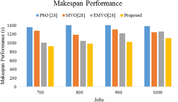

  

  Makespan performance for big-size task and varied VMs

• (b) Throughput Performance: Here, we present the throughput performance analysis for big-size dataset, where we have considered varied number of virtual machines based on the different sets of tasks. The obtained throughput is compared with other existing techniques as mentioned in Table 16.

  Table 16 Throughput performance for big size task and varied VMs

  Given Fig. 14 depicts the comparative analysis of throughput. The average throughput is obtained as 69.24, 77.54, 87.45 and 93.79 using PSO [28], MVO [28], EMVO [28], and Proposed approach, respectively.

  Fig. 14

  

  Throughput performance for big-size task and varied VMs

  This experiment shows that, the throughput performance of proposed approach is improved by 35.45%, 20.95%, and 7.24% when compared with aforementioned existing techniques.

• (c) Resource utilization Performance: Here, we present the comparative analysis for resource utilization for different virtual machines. Below given Table 17 shows the comparative analysis in terms of resource utilization.

  Table 17 Resource utilization performance for big size task and varied VMs

  Given Fig. 15 depicts the resource utilization performance. The average resource utilization performance is obtained as 98.40, 98.80, 98.40, and 99.28 using PSO [28], MVO [28], EMVO [28], and Proposed approach, respectively.

  Fig. 15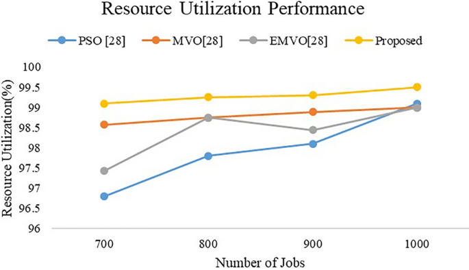

  

  Resource utilization for big-size task and varied VMs

  The resource utilization performance of proposed approach is improved by 0.89%, 0.48%, and 0.89% when compared with PSO [28], MVO [28] and EMVO [28].

  Finally, we present the comparative study in terms of energy consumption for varied number of tasks and virtual machines scenarios. Below given Fig. 16 depicts the energy consumption performance for varied number of tasks, where we have considered the total number of tasks as 200 to 1000. The obtained performance is compared with several scheduling schemes mentioned in [29].

  Fig. 16

  

  Energy consumption performance for varied number of tasks

  In this experiment, we obtained the average energy consumption as 4.48 J, 6.48 J, 5.7 J, 5.22 J, 4.58 J, 5.14 J, 5.34 J, 5.24 J, 4.34 J and 3 J by using MCT, SJFP, LJFP, Min–Min, Max–Min, PSO, SJFP-PSO, LJFP-PSO, MCT-PSO, and Proposed approach, respectively. Similarly, we measure the performance for varied number of virtual machines as depicted in Fig. 17.

  Fig. 17

  

  Energy consumption performance for varied number of virtual machines

  The average energy consumption is obtained as 3.64 J, 5.48 J, 4.81 J, 4.44 J, 3.88 J, 3.56 J, 5.06 J, 4.46 J, 3.36 J, and 2.14 J by using MCT, SJFP, LJFP, Min–Min, Max–Min, PSO, SJFP-PSO, LJFP-PSO, MCT-PSO, and Proposed approach for 40, 80, 120, 160, and 200 number of virtual machines, respectively. The experimental results show that, as the number of tasks, increasing along with the VMs, then the proposed approach balances load efficiently and utilizes resources efficiently. Moreover, this efficient utilization of resources and scheduling helps to minimize the energy consumption.

In these experiments, we obtained improved performance of makespan, throughput, resource utilization and energy consumption. The initial two parameters i.e., makespan and throughput satisfies the faster computing scenario which leads to complete the task in given deadline. The efficient task completion helps to minimize the energy consumption. Similarly, the better resource utilization reduces the resource wastages which lead towards the improving Quality of Service. Thus, the proposed approach is capable to reduce the energy consumption and improves overall performance of the cloud computing model.

5 Conclusion

In this work, we have focused on the energy consumption and task scheduling related issues of cloud computing. Task scheduling plays an important role in this field of cloud computing, which helps to obtain the efficient task allocation and minimizes the energy consumption. Several techniques have been presented in this field such as soft computing, optimization and machine learning, but the existing techniques suffer from various challenges. Thus, to overcome these issues, we present a novel scheme of task scheduling which adopts the reinforcement learning and a new solution is presented for reward mechanism and designing the policy. The experimental study shows that proposed approach achieves better performance when compared with existing task scheduling algorithms.

References

Pradeep, K., Jacob, T.P.: A hybrid approach for task scheduling using the cuckoo and harmony search in cloud computing environment. Wirel Pers. Commun. 101(4), 2287–2311 (2018)
Ebadifard, F., Babamir, S.M.: A PSO-based task scheduling algorithm improved using a load-balancing technique for the cloud computing environment. Concurr. Comput. 30(12), e4368 (2018)
Singh, P., Dutta, M., Aggarwal, N.: A review of task scheduling based on meta-heuristics approach in cloud computing. Knowl. Inf. Syst. 52(1), 1–51 (2017)
Madni, S.H.H., Abd Latiff, M.S., Abdullahi, M., Abdulhamid, S.I.M., Usman, M.J.: Performance comparison of heuristic algorithms for task scheduling in IaaS cloud computing environment. PLoS ONE 12(5), e0176321 (2017)
Shafiq, D.A., Jhanjhi, N.Z., Abdullah, A., Alzain, M.A.: A load balancing algorithm for the data centres to optimize cloud computing applications. IEEE Access 9, 41731–41744 (2021)
Chhabra, A., Singh, G., Kahlon, K.S.: Multi-criteria HPC task scheduling on IaaS cloud infrastructures using meta-heuristics. Clust. Comput. 24(2), 885–918 (2021)
Gani, A., Nayeem, G.M., Shiraz, M., Sookhak, M., Whaiduzzaman, M., Khan, S.: A review on interworking and mobility techniques for seamless connectivity in mobile cloud computing. J. Netw. Comput. Appl. 43, 84–102 (2014)
Ab-Rahman, N.H., Choo, K.K.R.: A survey of information security incident handling in the cloud. Comput. Secur. 49, 45–69 (2015)
Khan, S., Ahmad, E., Shiraz, M., Gani, A., Wahab, A.W.A., Bagiwa, M.A.: Forensic challenges in mobile cloud computing. Computer, Communications, and Control Technology (I4CT), 2014 International Conference on; 2014: IEEE.
Iqbal, S., Kiah, M.L.M., Dhaghighi, B., Hussain, M., Khan, S., Khan, M.K., et al.: On cloud security attacks: a taxonomy and intrusion detection and prevention as a service. J. Netw. Comput. Appl. 74, 98–120 (2016)
Han, S., Min, S., Lee, H.: Energy efficient VM scheduling for big data processing in cloud computing environments. J. Amb. Intell. Hum. Comput. 14, 1–10 (2019)
Kurp, P.: Green computing. Commun. ACM 51(10), 11–13 (2008)
https://www.computerworld.com/article/3089073/cloud-computing-slows-energy-demand-us-says.html
Zhang, J., Yu, F.R., Wang, S., Huang, T., Liu, Z., Liu, Y.: Load balancing in data center networks: a survey. IEEE Commun. Surv. Tutor. 20(3), 2324–2352 (2018)
Afzal, S., Kavitha, G.: Load balancing in cloud computing: a hierarchical taxonomical classification. J. Cloud Comput. 8(1), 1–24 (2019)
Arunarani, A.R., Manjula, D., Sugumaran, V.: Task scheduling techniques in cloud computing: a literature survey. Futur. Gener. Comput. Syst. 91, 407–415 (2019)
Alworafi, M. A., Dhari, A., El-Booz, S. A., Nasr, A. A., Arpitha, A., & Mallappa, S.: An enhanced task scheduling in cloud computing based on hybrid approach. In: Data Analytics and Learning (pp. 11–25). Springer, Singapore (2019)
Liu, L., & Qiu, Z.: A survey on virtual machine scheduling in cloud computing. In 2016 2nd IEEE International Conference on Computer and Communications (ICCC) (pp. 2717–2721). IEEE. (2016)
Zakarya, M.: An extended energy-aware cost recovery approach for virtual machine migration. IEEE Syst. J. 13(2), 1466–1477 (2018)
Alkayal, E. S., Jennings, N. R., & Abulkhair, M. F.: Survey of task scheduling in cloud computing based on particle swarm optimization. In 2017 International Conference on Electrical and Computing Technologies and Applications (ICECTA) (pp. 1–6). IEEE. (2017)
Tong, Z., Deng, X., Chen, H., Mei, J., Liu, H.: QL-HEFT: a novel machine learning scheduling scheme base on cloud computing environment. Neural Comput. Appl. 15, 1–18 (2019)
Sharma, M., Garg, R.: An artificial neural network based approach for energy efficient task scheduling in cloud data centers. Sustain. Comput. 26, 100373 (2020)
Rjoub, G., Bentahar, J., Abdel Wahab, O., Saleh Bataineh, A.: Deep and reinforcement learning for automated task scheduling in large-scale cloud computing systems. Concurr. Comput. 15, 5919 (2020)
Mansouri, N., Zade, B.M.H., Javidi, M.M.: Hybrid task scheduling strategy for cloud computing by modified particle swarm optimization and fuzzy theory. Comput. Ind. Eng. 130, 597–633 (2019)
Negi, S., Rauthan, M.M.S., Vaisla, K.S., Panwar, N.: CMODLB: an efficient load balancing approach in cloud computing environment. J Supercomput. 12, 1–53 (2021)
Sulaiman, M., Halim, Z., Lebbah, M., Waqas, M., Tu, S.: An evolutionary computing-based efficient hybrid task scheduling approach for heterogeneous computing environment. J. Grid Comput. 19(1), 1–31 (2021)
Shukri, S.E., Al-Sayyed, R., Hudaib, A., Mirjalili, S.: Enhanced multi-verse optimizer for task scheduling in cloud computing environments. Expert Syst. Appl. 15, 114230 (2020). https://doi.org/10.1016/j.eswa.2020.114230
Alsaidy, S. A., Abbood, A. D., & Sahib, M. A.: Heuristic initialization of PSO task scheduling algorithm in cloud computing. J. King Saud Univ. Comput. Inform. Sci. (2020)
Ding, D., Fan, X., Zhao, Y., Kang, K., Yin, Q., Zeng, J.: Q-learning based dynamic task scheduling for energy-efficient cloud computing. Futur. Gener. Comput. Syst. 108, 361–371 (2020)
Hoseiny, F., Azizi, S., Shojafar, M., Tafazolli, R.: Joint QoS-aware and cost-efficient task scheduling for fog-cloud resources in a volunteer computing system. ACM Trans. Internet Technol. (TOIT) 21(4), 1–21 (2021)
Abualigah, L., Diabat, A.: A novel hybrid antlion optimization algorithm for multi-objective task scheduling problems in cloud computing environments. Clust. Comput. 24(1), 205–223 (2021)
Hoseiny, F., Azizi, S., Shojafar, M., Ahmadiazar, F., & Tafazolli, R.: PGA: a priority-aware genetic algorithm for task scheduling in heterogeneous fog-cloud computing. In IEEE INFOCOM 2021-IEEE Conference on Computer Communications Workshops (INFOCOM WKSHPS) (pp. 1–6). IEEE. (2021)
Calzarossa, M.C., Della Vedova, M.L., Massari, L., Nebbione, G., Tessera, D.: Multi-objective optimization of deadline and budget-aware workflow scheduling in uncertain clouds. IEEE Access 9, 89891–89905 (2021)
Beloglazov, A., Buyya, R., Lee, Y. C., & Zomaya, A.: A taxonomy and survey of energy-efficient data centers and cloud computing systems. In Advances in computers (Vol. 82, pp. 47–111). Elsevier (2011).
Funding
None.
Author information
Authors and Affiliations
Corresponding author
Ethics declarations
Conflict of interest
Additional information
Publisher's Note
Springer Nature remains neutral with regard to jurisdictional claims in published maps and institutional affiliations.
Rights and permissions
About this article
Cite this article
Siddesha, K., Jayaramaiah, G.V. & Singh, C. A novel deep reinforcement learning scheme for task scheduling in cloud computing. Cluster Comput 25, 4171–4188 (2022). https://doi.org/10.1007/s10586-022-03630-2
Received:
Revised:
Accepted:
Published:
Issue Date:
DOI: https://doi.org/10.1007/s10586-022-03630-2