Finding exoplanets using object detection

Abstract

Since the initial finding of exoplanets, planet detection has gained prominence as a field of research in astronomy. Using a variety of techniques, including gravitational microlensing, direct imaging, astrometry, and the radial velocity approach, more than 5,000 exoplanets have been found. The majority of confirmed exoplanet discoveries, have been made using the transit method. The machine learning (ML) models used in earlier approaches for prediction of exoplanets involve usage of large datasets and complex architectures, which takes a lot of time for training and hence detection of exoplanets.

This work has presented a novel exoplanet detection approach based on the Object Detection algorithm- You only look once (YOLO). The data was collected for 221 confirmed exoplanets detected by Telescope and Transiting Exoplanet Survey Satellite (TESS) and light curves were downloaded for the same. The annotations were generated around the brightness dips in the light curves, followed by YOLO-object detection. The presented work not only predicts the dips in brightness in the light curve accurately but also takes less time to train the proposed model.

The work has achieved a mAP 0.5 of 0.82, a precision of 0.85, and a recall of 0.81. Additionally, a comparison of YOLO, MobileNet-SSDv2, and EfficientDet Lite is presented. The EfficientDet Lite D2 scores mAP0.5 0.66 and Average Recall 0.56, which is very satisfactory considering it is running on low computing power devices such as mobile phones, Raspberry Pi and other microcomputers.

1 Introduction

Are we alone? Is there any other planet like Earth in the universe? This is a uniquely human question that has deep roots in all of us and probably originated when humanity first looked up at the stars in the night sky.

Multidisciplinary science that includes astronomy, astrobiology, geology, planetary science, and much more. Exoplanet detection started about 25 years ago and continues to give hope for the diversity of the world, well beyond our solar system. The rapid unearthing of exoplanets has broadened the field of scientific possibilities. This research problem drives an understanding of planetary processes outside the solar system, and finding exoplanets opens up vast exploration areas to look for other habitable planets (Chickles 2021; Azari et al. 2020; Cannon et al. 2022).

With recent technological advances and the use of sophisticated telescopes such as NASA’s Kepler Space Telescope and Transiting Exoplanet Survey Satellite (TESS) (Yu et al. 2019), scientists can now scan stars in the visible cosmos to check if they have extrasolar planets (called “exoplanets”). Depending on the diameter of the planet(stars), a planet may travel in front of its host star, obscuring a portion of the star’s light and causing the pragmatic visual illumination of the star to decline by a tiny amount. So, for the transit method, a star’s brightness is constantly measured, and “dips” in the light curves are looked for.

One downside of this approach is that transits can only be witnessed once the planet’s circle exactly aligned with the position of the observer. Another worry is the high number of false detections, which can be caused by binary systems or asteroids that pass in front of each other. This means that findings need to be backed up by more evidence.

This work is aimed at combining observations from light curves of 221 confirmed exoplanets using an object detection technique, paving the way for a broader area of exoplanet study, including planet size and characteristics. The work deals with the following points: i) To come up with an algorithm that can accurately detect dips in light curves with a minimum number of false positives. ii). To introduce simpler or less computationally intensive ways of exoplanet detection that perform similarly well or better than existing approaches. iii). To do a comparative study between a few object detection algorithms to determine the most efficient one.

2 Literature review

(Wright and Gaudi 2012) research looked at several observational methods for finding planetary companions to stars, with a focus on radial velocities, imaging, astrometry etc. For each technique, this document derives or summarises the main observable phenomena utilised to deduce the reality of planetary partners, planet and star features that may be determined from the size of these signals. This study then compares the amount of the common causes of measurement error to the total experimental requirements for robustly identifying signals using each technique. Whereas (Botros 2014) performs the basic analytics technique like preprocessing, feature extraction on Kepler Telescope light curves for binary classification of exoplanets. There system generates 85 percent accuracy. To improve the accuracy further, the proposed method works on Roboflow technique to do real time object detection

(Malik et al. 2022) presents a traditional machine learning (ML), appeal in finding a planet. The solution involves autonomously collecting time series characteristics from light curves and feeding them into a gradient enhanced trees model. The research shows that ML approaches can recognize light curves containing planet signals more reliably than BLS while dramatically lowering the amount of false positives. They able to predict a planet with an AUC of 0.94. To further enhance the accuracy, the proposed work used YOLO model, which takes lesser training time with near equal results.

The study (Pearson et al. 2018) demonstrates the use of an artificial neural network to study the photometric features of a transiting exoplanet. As neural networks are discriminative, they can only provide a qualitative evaluation of the candidate signal by predicting the likelihood of sensing a transportation within a subset of the given time sequence. They used periodic transits by employing a phase folding approach that provides a constraint when fitting for the orbital period of planet signals that are shorter than the noise

(Chintarungruangchai and Jiang 2019) used a light curve from the Kepler Space Telescope and deep-learning models were created and tested. According to the research, folding can help retain high accuracy. Even when Signal to noise (S/N) is less than 10, all models with folding may achieve more than 98 percent accuracy. They show that the 2D-CNN-folding-2 model has good value even when the folding time differs from the transit length by 20%.

(Shallue and Vanderburg 2018) presented a deep learning-based technique for identifying Kepler transiting planet candidates automatically. The neural network method can determine the difference among transiting exoplanets and false positives (FP) such as eclipsing binaries, observational artefacts, and stellar variability. On the test set, the model ranks true planet candidates above FP 98.8 percent of the time. While the model improves simulated planets at a decent rate on simulated data, it fails to reject several kinds of simulated FP, such as weak secondary eclipses, as well as the more mature Robovetter system.

To further enhance the accuracy and to reduce the time consumption, the propose work divides confirmed images of exoplanet light curves into a grid of cells, with each cell immediately predicting a bounding box around the dip and dip categorization.

3 Proposed solution

Data in astronomy is rapidly expanding thanks to new and advanced telescopes. Traditional procedures based on inefficient human judgments that vary depending on the investigating expert. The YOLO Object detection model trains on the dataset of light curves of 221 confirmed exoplanets based on the brightness dips. The dataset is downloaded from the TESS Input Catalog (TIC) ID’s of the confirmed exoplanet sites (NASA 2022 & Berrios et al. 2021) https://exoplanetarchive.ipac.caltech.edu/, which is a NASA Exoplanet Archive. The TIC ID aids in the determination of both physical and observational parameters of planet candidates. It is intended for use by both the TESS research team and the general public, and it is regularly updated. Figure 1 shows the image of a light curve.

Fig. 1

Image of a light curve

To perform the computation more effectively the work has incorporated following tools and methods

• i. LabelImg- It is an annotation tool for graphical images. This has been used to annotate, drawing bounding boxes around brightness dips of the confirmed set of exoplanets. Figure 2, illustrate the light curve after annotate.

  Fig. 2

  

  Annotated light curve

• ii. Roboflow has been used for real time object detection and it also makes things easy/simple/clean by the following:

  • Creates simple and effective file structure of train test validation sets that aids in training.

  • Creating train test validation sets

  • Resizing of image data and transforming or cleaning the data.

  • Converting data to suitable formats required to train object detection models.

• iii. Weights & Biases (WB) is used for experiment tracking, dataset versioning, and collaborating on ML. It is basically used for visualizing all the data that the model outputs.

3.1 Proposed architecture

The presented work architecture is shown in Fig. 3, which consists of the YOLOv1 architecture (Redmon et al. 2016) and other subsequent models. Here, the input image is divided into a GSxGS grid by the system. Each grid cell forecasts bounding boxes (around the bright-ness dips) and their confidence ratings; these scores give certainty that the box contains the dip (the object) and the accuracy of the predicted result. Each bounding box (He et al. 2019; Świeżewsk 2022) around the dip is represented using a 5-D vector:

Fig. 3

Exoplanet detection using YOLOv1

• the box’s middle (bmX, bmY)

• Width (bmW)

• Height (bmH), a value denoting the object’s class with the letter “c” (dog, cat..)

• A probability of an item being present in the box, represented by the value “pc”

The ‘C’ conditional class probabilities, Prob(Class-Object), are also detected for respectively grid cell. These probabilities depend on the grid cell in which an object(dip) is situated. Irrespective of the number of bounding boxes, they only estimate 1 set of class probabilities per grid cell (Redmon et al. 2016). They multiply the discrete box confidence, predict with the conditional class probabilities. This provides with scores for every box in the class. These scores encode the probability of that class presence in the box as well as how well the projected box matches the item.

As each cell predicts an output, the number of anticipated boxes might grow excessive, and the majority of them will be empty. To address this issue, the technique employs the Non-Max Suppression algorithm to delete boxes based on ‘pc’ that do not contain any objects (Redmon et al. 2016 & Świeżewsk 2022).

3.2 Object detection model construction

Object detection is a computer vision task that includes both localising and categorising one or more dips within a picture of verified light curves. It is a computer vision problem that requires both effective dip localization (finding and drawing a bounding box around each dip in the image of the light curve) and successful object classification (predicting the proper class of dip that was localised), which aids in predicting the planet’s likelihood of being an exoplanet.

3.2.1 Data pre-processing and annotations

The data being used is the TIC ID of the 221 confirmed exoplanets. To detect the planets, the TESS satellite employs a technique known as the transit method. TESS monitors a star for 27.4 days, and if any planet orbiting the star passes in front of it, that is, between the satellite and the star, the brightness of the star decreases, which is detected and displayed in a graph called the light curve.

LabelImg has been used for annotations. It is a free, open-source tool for graphically labelling images(light curves of 221 confirmed exoplanets). It’s written in Python and uses QT for its graphical interface. Bounding boxes have been created across the prominent dips for the generated light curve images.

3.2.2 Data compatibility using roboflow

Roboflow is used here to convert the data into a compatible format for YOLO V3 and YOLO V5. Roboflow makes it simpler by cheating on training test validation sets and helps resize the image data from the light curves and cleaning of data. Roboflow is a computer vision platform that allows us to create training-ready datasets for the YOLO models more rapidly and accurately by improving data collection, preprocessing, and model training by transforming the data to a suitable format for YOLO versions V3 and V4.

Users may use Roboflow to upload custom datasets, draw annotations, adjust image orientations, and resize photos to improve compliance with the models used for training. It may also be used to upload custom datasets, change image contrast, alteration image orientations, resize, and perform data augmentation and model training.

Object detection model training using Roboflow train: models may also be trained using it and this report uses Roboflow train to train on the annotated images of the light curves of 221 confirmed exoplanets. The Roboflow training turned our dataset into a compatible format and has the following advantages.

• Improved model performance for (YOLO V3 and YOLO V5).

• Easy training and streamlined deployment.

• Active and real time learning (Object detection).

3.2.3 Object detection using YOLO

The “You Only Look Once,” or YOLO, family of models is a set of end-to-end deep learning models developed by Joseph Redmon for quick object recognition.

YOLO causes more localization errors but predicts fewer FP in the related. Finally, YOLO learns extremely broad illustrations of objects. It outperforms other detection algorithms like DPM and R-CNN. Using transfer learning, the model trained YOLOv3 and YOLOv5 using the Ultralytics framework.

3.2.4 Proposed model training - epochs

The initial YOLO model versions provided a wide architecture, whereas the second refined the design and employed preset anchor boxes to improve bounding box suggestion around brightness dips, and the final the third expanded the model architecture and training procedure. The latest version V5 has shown to be more exact and efficient for predicting brightness dips from light curves, resulting in better exoplanet prediction.

Training had been done for YOLO version 3 and YOLO version 5. For version 3, the model has been trained on 100 and 150 epochs as shown in Fig. 4 & 5. For YOLO version V5, the model has been trained for 100 epochs as shown in Fig. 6.

Fig. 4

Detection of dips using YOLOv3 for 100 Epochs

Fig. 5

Detection of dips using YOLOv3 for 150 Epochs

Fig. 6

Detection of dips using YOLOv5 for 100 Epochs

Roboflow, It has the ability to resize images to be compatible with the versions of YOLO used for a general comparison on the efficiency.

3.2.5 Detection of dips

The Object detection method makes use of a single deep convolutional neural network (first a version of GoogLeNet, then modified and named DarkNet based on VGG) that divides confirmed images of exoplanet light curves into a grid of cells, with each cell immediately predicting a bounding box around the dip and dip categorization.

As a consequence, a huge number of potential bounding boxes are generated and this constitutes a part of the annotations, which are then aggregated into a final forecast of the prediction of dips via a post-processing phase.

Figure 4 & 6 are the detection’s made for a test image using VOLO v3 with 100 & 150 epochs. Similarly Fig. 6 shows VOLO v 5 with 100 epochs. By observing the light curve of Fig. 4, 5 and 6, author has notice that the v3 is unable to predict all four dips, whereas v5 is able to predict all the four dips.

3.2.6 Exoplanet classification

The proposed model is applied to TESS data. As the length is supplied, the most significant drop may be automatically recognised, allowing for a better understanding for categorizing it as an exoplanet. Other ML models are typically black boxes with difficult to anticipate outcomes. Here Roboflow train is used to make the annotated data in a compatible format for the YOLO model.

Thereafter the work has further compared with MobileNet–SSDV2 and Efficient Det-Lite. Here MobileNet–SSDV2 uses two different kinds of blocks. Block one is a residual block with a stride of one. Another block is for downsizing with a stride of two. For both kinds of blocks, there are three levels. 1 × 1 convolution with ReLU6 makes up the first layer. The depthwise convolution is the second layer. The third layer is 1 × 1 convolution once more, but this time there is no non-linearity.

Subsequently to run object detection model on low power devices such as mobile phone, Raspberry Pi, author has incorporated EfficientDet-Lite which is built specifically to run object detection models on low-power devices. This work compares EfficientDet-Lite-D0 and EfficientDet-Lite-D2 for 150 and 100 epcohs, respectively.

4 Results and discussion

The proposed work is validated using matrices and statistical measures such as mAP, Precision, Recall and F1 using YOLO v3, YOLO v5, Mobile NET-SSDV 2 and Efficient DET-LITE - D0 & D2 as shown in Table 1.

Table 1 Results of mAP, Precision, Recall and F1 using YOLO v3, YOLO v5, Mobile NET-SSDV 2 and Efficient DET-LITE (D0 & D2)

Mean average precision

In Fig. 7, blue and red lines denote the results of YOLO V3 for 100 and 150 epochs respectively. The mAP 0.5 shows the performance of the model at IOU threshold of 0.5, which implies that 50% of the predicted bounding boxes along the dips overlap with the ground truth box. It can be concluded from the graphs of both the YOLO versions that mAP of version 5 is higher than version 3 and hence is a better performing model. Similarly Fig. 8, blue and green lines denote the result of YOLO V5 during 1st and 2nd run respectively.

Fig. 7

Mean Average Precision using YOLOv3 for 100 epochs (blue line) and 150 epochs (red line)

Fig. 8

YOLOv5 mAP Mean Average Precision using YOLOv5 for 1st run (blue line) and 2nd run (green line)

Precision

Precision for YOLO v5 is 0.83. Thus, 83% of all the dips predicted by the model are confirmed. Figure 9 shows the precision for YOLO v3 is 0.6. here, 63% of all the dips predicted by the model are confirmed. Result shows that version 5 has a higher precision of 0.83 which results in better prediction as displayed in Fig. 10.

Fig. 9

Precision graph using YOLOv3, here blue line represents 100 epochs and red line represents 150 epochs

Fig. 10

Precision graph using YOLOv5, here blue line represents 1st run and red line represents 2nd run

Recall

Recall for YOLO V3 is 0.6 which is comparatively much lower and hence it accurately predicts 60% out of the set as displayed in Fig. 11. Whereas recall value for YOLO V5 is greater than 0.8, which implies that the suggested model is able to predict more than 80% out of all the dips as shown in Fig. 12.

Fig. 11

Recall graph using YOLOv3, here blue line signifies 100 epochs whereas red line 150 epochs

Fig. 12

Recall graph using YOLOv5, here blue line represents 1st run and red line signifies 2nd run

Meanwhile the most complex CNN models are able to achieve this rate compared to the suggested model which is less complex and takes less time and does more training

Training losses

Training losses correspond to the model’s predicted values to the actual values or the true values. This helps with a more competitive study between both the versions of YOLO. The models are trained on 100 and 150 epochs. As the validation loss starts to plateau, the test is not performed for a greater number of epochs. This will only result in an increment of the validation loss, which is not required.

• Train/box loss: The proposed model predicts the bounding boxes across the dips. The box loss metric gives a classification as to how distinct the predicted box is compared to the ground truth box as displayed in Fig. 13.

  Fig. 13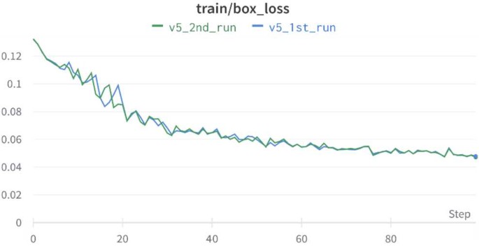

  

  Computation of box loss using YOLOv5

• Train/Object loss: The proposed model predicts the object(dip) inside the bounding boxes. The object loss metric gives a difference between a model’s predicted value and its true value as shown in Fig. 14.

  Fig. 14

  

  Computation of obj loss using YOLOv5

• Train/class loss: As it can be observed from the previous figures, there is only one class to be predicted and hence the cls loss graph is a constant like at 0 as show in Fig. 15.

  Fig. 15

  

  Computation of cls loss using YOLOv5

Box loss is low for YOLOv5 and tends to decrease giving the model better accuracy for the prediction. It also indicates that the predicted bounding boxes are similar to ground truth boxes.

The object loss also tends to decrease. The result concludes that the graph obtained from both the YOLO models state that v5 has lower training losses overall and thus gives a more accurate prediction of the brightness dips.

5 Conclusion and future scope

Object detection models have advanced rapidly in the previous decade, and they are now an integral element of our way of functioning. The majority of confirmed exoplanet discoveries, have been made using the transit method. This work presents a novel approach to detecting exoplanets using the object detection YOLO model. The model has been trained on the light curves of 221 confirmed exoplanets, it is successfully able to detect the brightness dips. In comparison to the Mobile NET-SSDV 2 and Efficient DET-LITE (D0 & D2) models. on ML-TESS data. Subsequently YOLO V5 GPU metric signifies that the smaller amount of data gives a better output by drawing boundary boxes around the dips, which thus gives a better way of analyzing. Further, the EfficientDet-Lite and MobileNet-SSDv2 object detection models were evaluated in this study. The comparative study between the different versions of YOLO models shows the competency of YOLO V5, giving a precision of 0.856 which is atleast 15% better than the other models. However, the applications of the presented model can be extended to determining the planet size/radius as an output based on the length of the “dip” detected.

References

Azari, A.R., Biersteker, J.B., Dewey, R.M., Doran, G., Forsberg, E.J., Harris, C.D., et al.: Integrating machine learning for planetary science: Perspectives for the next decade (2020). ArXiv preprint. arXiv:2007.15129
Berrios, D.C., Galazka, J., Grigorev, K., Gebre, S., Costes, S.V.: NASA GeneLab: interfaces for the exploration of space omics data. Nucleic Acids Res. 49(D1), D1515–D1522 (2021)
Botros, A.: Artificial intelligence on the final frontier: using machine learning to find new earths. Technical report, Stanford University (2014)
Cannon, M., Kelly, A., Freeman, C.: Implementing an open & FAIR data sharing policy—a case study in the Earth and environmental sciences. Learn. Publ. 35(1), 56–66 (2022)
Chickles, E.T.: Applications of Convolutional Neural Networks to Problems in Astronomy and Planetary Science (2021)
Chintarungruangchai, P., Jiang, G.: Detecting exoplanet transits through machine-learning techniques with convolutional neural networks. Publ. Astron. Soc. Pac. 131(1000), 064502 (2019)
He, Y., Zhu, C., Wang, J., Savvides, M., Zhang, X.: Bounding box regression with uncertainty for accurate object detection. In: Proceedings of the IEEE/CVF Conference on Computer Vision and Pattern Recognition, pp. 2888–2897 (2019)
Malik, A., Moster, B.P., Obermeier, C.: Exoplanet detection using machine learning. Mon. Not. R. Astron. Soc. 513(4), 5505–5516 (2022)
NASA Exoplanet Archive (2022). https://exoplanetarchive.ipac.caltech.edu/. Dataset
Pearson, K.A., Palafox, L., Griffith, C.A.: Searching for exoplanets using artificial intelligence. Mon. Not. R. Astron. Soc. 474(1), 478–491 (2018)
Redmon, J., Divvala, S., Girshick, R., Farhadi, A.: You only look once: unified, real-time object detection. In: Proceedings of the IEEE Conference on Computer Vision and Pattern Recognition, pp. 779–788 (2016)
Shallue, C.J., Vanderburg, A.: Identifying exoplanets with deep learning: a five-planet resonant chain around Kepler-80 and an eighth planet around Kepler-90. Astron. J. 155(2), 94 (2018)
Świeżewsk, J.: Algorithm and YOLO object detection (2022). https://appsilon.com/object-detection-yolo-algorithm/
Wright, J.T., Gaudi, B.S.: Exoplanet detection methods (2012). ArXiv preprint. arXiv:1210.2471
Yu, L., Vanderburg, A., Huang, C., Shallue, C.J., Crossfield, I.J., Gaudi, B.S., et al.: Identifying exoplanets with deep learning. III. Automated triage and vetting of TESS candidates. Astron. J. 158(1), 25 (2019)
Acknowledgements
Not applicable.
Funding
Author information
Authors and Affiliations
Contributions
All authors has contributed equally.
Corresponding author
Ethics declarations
Competing interests
The authors declare no competing interests.
Additional information
Publisher’s Note
Springer Nature remains neutral with regard to jurisdictional claims in published maps and institutional affiliations.
Rights and permissions
Springer Nature or its licensor (e.g. a society or other partner) holds exclusive rights to this article under a publishing agreement with the author(s) or other rightsholder(s); author self-archiving of the accepted manuscript version of this article is solely governed by the terms of such publishing agreement and applicable law.
About this article
Cite this article
Sekhar, S.R.M., Tejas, C., Kanna, V.S.N. et al. Finding exoplanets using object detection. Astrophys Space Sci 368, 75 (2023). https://doi.org/10.1007/s10509-023-04232-z
Received:
Accepted:
Published:
DOI: https://doi.org/10.1007/s10509-023-04232-z