Semantic Factorization and Descent

Abstract

Let ${\mathbb {A}}$ be a 2-category with suitable opcomma objects and pushouts. We give a direct proof that, provided that the codensity monad of a morphism p exists and is preserved by a suitable morphism, the factorization given by the lax descent object of the two-dimensional cokernel diagram of p is up to isomorphism the same as the semantic factorization of p, either one existing if the other does. The result can be seen as a counterpart account to the celebrated Bénabou–Roubaud theorem. This leads in particular to a monadicity theorem, since it characterizes monadicity via descent. It should be noted that all the conditions on the codensity monad of p trivially hold whenever p has a left adjoint and, hence, in this case, we find monadicity to be a two-dimensional exact condition on p, namely, to be an effective faithful morphism of the 2-category ${\mathbb {A}}$.

1 Introduction

Grothendieck descent theory [7] has been generalized from a solution of the problem of understanding the image of the functors ${\textsf {Mod}}(f)$ in which ${\textsf {Mod}}:{\textsf {Ring}}\rightarrow {\textsf {Cat}}$ is the usual pseudofunctor between the category of rings and the 2-category of categories that associates each ring $\mathcal {R}$ with the category ${\textsf {Mod}}( \mathcal {R})$ of right $\mathcal {R}$-modules (e.g. [10]).

It is often more descriptive to portray descent theory as a higher dimensional counterpart of sheaf theory (see, for instance, the introduction of [8]). In this context, the analogy can be roughly stated as follows: the descent condition and the descent data are respectively two-dimensional counterparts of the sheaf condition and the gluing condition.

The most fundamental constructions in descent theory are the lax descent category and its variations (e.g. [28, pag. 177]). Namely, given a truncated pseudocosimplicial category

we construct its lax descent category or descent category. An object of the lax descent category (descent category) is an object x of the category $\mathcal {A}(\textsf {1} )$ endowed with a descent data which is a morphism (respectively, invertible morphism) $\mathcal {A}(d^1)(x)\rightarrow \mathcal {A}(d^0)(x)$ satisfying the usual cocycle/associativity and identity conditions. Morphisms are morphisms between the underlying objects in $\mathcal {A}(\textsf {1} )$ that respect the descent data.

Another perspective, which highlights descent theory’s main role in Janelidze-Galois theory, is that, given a bifibred category, the lax descent category of the truncated pseudocosimplicial category induced by an internal category generalizes the notion of the category of internal (pre)category actions (e.g. [9, Section 1]).

In the setting above, if the bifibration is the basic one, we actually get the notion of internal actions. The simplest example is the category of actions of a small category in ${\textsf {Set}}$; that is to say, the category of functors from a small category into ${\textsf {Set}}$. A small category a is just an internal category in ${\textsf {Set}}$ and the category of actions (functors) $a\rightarrow {\textsf {Set}}$ coincides with the lax descent category of the composition of the (image by $\textrm{op}: {\textsf {Cat}}^\text {co} \rightarrow {\textsf {Cat}}$ of the) internal category a, $\textrm{op}(a): \Delta _\text {3} \rightarrow {\textsf {Set}}^\textrm{op}$, with the pseudofunctor ${\textsf {Set}}/ -:{\textsf {Set}}^\textrm{op}\rightarrow {\textsf {Cat}}$ that comes from the basic fibration.

Assume that we have a pseudofunctor $\mathcal {F}: {\mathbb {C}} ^\textrm{op}\rightarrow {\textsf {Cat}}$ such that ${\mathbb {C}}$ has pullbacks, and $\mathcal {F}(q)!\dashv \mathcal {F}(q)$ for every morphism q of ${\mathbb {C}}$. Given a morphism $q: w\rightarrow w'$ of ${\mathbb {C}}$, the Bénabou–Roubaud theorem (see [4] or, for instance, [19, Theorem 1.4]) says that the (lax) descent category of the truncated pseudocosimplicial category

given by the composition of $\mathcal {F}$ with the internal groupoid induced by q, is equivalent to the Eilenberg–Moore category of the monad induced by the adjunction $\mathcal {F}(q)!\dashv \mathcal {F}(q)$, provided that $\mathcal {F}$ satisfies the so called Beck-Chevalley condition (see, for instance, the Beck-Chevalley condition for pseudofunctors in [21, Section 4]).

Since monad theory already was a established subfield of category theory, the Bénabou–Roubaud theorem gave an insightful connection between the theories, motivating what is nowadays often called monadic approach to descent by giving a characterization of descent via monadicity in several cases of interest (see, for instance, [24, Section 1], [8, Section 2], or the introduction of [19]).

The main contribution of the present article can be seen as a counterpart account to the Bénabou–Roubaud theorem. We give the semantic factorization via descent, hence giving, in particular, a characterization of monadicity via descent. Although the Bénabou–Roubaud theorem is originally a result in the setting of the 2-category ${\textsf {Cat}}$, our contribution takes place in the more general context of two-dimensional category theory (e.g. [12]), or in the so called formal category theory, as briefly explained below.

In his pioneering work on bicategories, Bénabou observed that the notion of monad, formerly called standard construction or triple, coincides with the notion of a lax functor $\textsf {1}\rightarrow {\textsf {Cat}}$ and can be pursued in any bicategory, giving convincing examples to the generalization of the notion [3, Section 5].

Taking Bénabou’s point in consideration, Street [25, 26] gave a formal account and generalization of the former established theory of monads by developing the theory within the general setting of 2-categories. The formal theory of monads is a celebrated example of how two-dimensional category theory can give insight to 1-dimensional category theory, since, besides generalizing several notions, it conceptually enriches the formerly established theory of monads. Street [25] starts showing that, when it exists, the Eilenberg–Moore construction of a monad in a 2-category ${\mathbb {A}}$ is given by a right 2-reflection of the monad along a 2-functor from the 2-category ${\mathbb {A}}$ into the 2-category of monads in ${\mathbb {A}}$. From this point, making good use of the four dualities of two-dimensional category theory, Street develops the formal account of aspects of monad theory, including distributive laws, Kleisli construction, and a generalization of the semantics-structure adjunction (e.g. [5, Chapter II]).

The theory of two-dimensional limits (e.g. [11, 28]), or weighted limits in 2-categories, also provides a great account of formal category theory, since it shows that several constructions previously introduced in 1-dimensional category theory are actually examples of weighted limits and, hence, are universally defined and can be pursued in the general context of a 2-category.

Examples of the constructions that are particular weighted limits are: the lax descent category and variations, the Eilenberg–Moore category [6, Theorem 2.2] and the comma category [15, pag. 36]. Duality also plays important role in this context: it usually illuminates or expands the original concepts of 1-dimensional category theory. For instance:

• The dual of the notion of descent object gives the notion of codescent object, which is important, for instance, in 2-dimensional monad theory (see, for instance, [14, 17, 18]);

• The dual notion of the Eilenberg–Moore object in ${\textsf {Cat}}$ gives the Kleisli category [13] of a monad, while the codual gives the category of the coalgebras of a comonad.

Despite receiving less attention in the literature than the notion of comma object, the dual notion, called opcomma object, was already considered in [27, pag. 109] and it is essential to the present work. More precisely, given a morphism $p: e\rightarrow b$ of a 2-category ${\mathbb {A}}$, if ${\mathbb {A}}$ has suitable opcomma objects and pushouts, on one hand, we can consider the two-dimensional cokernel diagram

of p, whose precise definition can be found in 2.9 below. Assuming that ${\mathbb {A}}$ has the lax descent object of $\mathcal {H}_p$, the universal property of $\text {lax}\text {-}\mathcal {D}\text {esc}\left( \mathcal {H}_p\right)$ and the universal 2-cell of the opcomma object induce a factorization

of p, called herein the semantic lax descent factorization. If the comparison morphism $e\rightarrow \text {lax}\text {-}\mathcal {D}\text {esc}\left( \mathcal {H}_p \right)$ is an equivalence, we say that p is an effective faithful morphism. This concept is actually self-codual, meaning that its codual notion coincides with the original one.

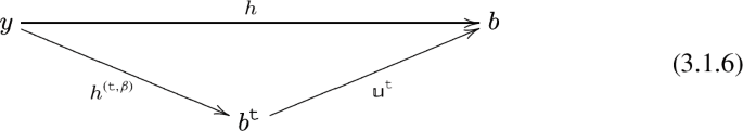
On the other hand, if such a morphism p has a codensity monad $\texttt {t}$ which means that the right Kan extension of p along itself exists in ${\mathbb {A}}$, then the universal 2-cell of the $\textrm{ran}_p p$ induces the semantic factorization

through the Eilenberg–Moore object $b^\texttt {t}$ of $\texttt {t}$ provided that it exists (see, for instance, [5, pag. 67] for the case of the 2-category of enriched categories). If the comparison $e\rightarrow b ^\texttt {t}$ is an equivalence, we say that p is monadic. The codual notion is that of comonadicity.

The main theorem of the present article concerns both the factorizations above. More precisely, Theorem 4.8 states the following:

Main Theorem: 1

Let ${\mathbb {A}}$ be a 2-category which has the two-dimensional cokernel diagram of a morphism p. Moreover, assume that $\textrm{ran}_p p$ exists and is preserved by the universal morphism $\delta _ {p\uparrow p} ^0$ of the opcomma object $b\uparrow _p b$.

There is an isomorphism between the Eilenberg–Moore object $b ^\texttt {t}$ and the lax descent object $\text {lax}\text {-}\mathcal {D}\text {esc}\left( \mathcal {H}_p \right)$, either one existing if the other does. In this case, the semantic factorization (SF) is isomorphic to the semantic lax descent factorization (SLDF).

In particular, this gives a formal monadicity theorem as a corollary, since it shows that, assuming that a morphism p of ${\mathbb {A}}$ satisfies the conditions above on the codensity monad, p is monadic if and only if p is an effective faithful morphism. Moreover, since this result holds for any 2-category, we can consider the duals of this formal monadicity theorem: namely, we also get characterizations of comonadic, Kleisli and co-Kleisli morphisms.

By the Dubuc-Street formal adjoint-functor theorem (viz., [5, Theorem I.4.1] and [30, Prop. 2]), if p has a left adjoint, the codensity monad is the monad induced by the adjunction and $\textrm{ran}_p p$ is absolute. Thus, in this case, assuming the existence of the two-dimensional cokernel diagram, the hypothesis of our theorem holds. Therefore, as a corollary of our main result, we get the following monadicity characterization:

Monadicity Theorem:

Assume that the 2-category ${\mathbb {A}}$ has the two-dimensional cokernel diagram of $p: e\rightarrow b$.

• The morphism p is monadic if and only if p is an effective faithful morphism and has a left adjoint;

• The morphism p is comonadic if and only if p is an effective faithful morphism and has a right adjoint.

Recall that, in the particular case of ${\mathbb {A}}= {\textsf {Cat}}$ (and other 2-categories, such as the 2-category of enriched categories), we have Beck’s monadicity theorem (e.g. [2, Theorem 3.14] and [5, Theorem II.2.1]). It states that: a functor is monadic if and only if it creates absolute coequalizers and it has a left adjoint. Hence, by our main result, we can conclude that: provided that the functor p has a left adjoint, p creates absolute coequalizers if and only if it is an effective faithful morphism.

The fact above suggests the following question: are effective faithful morphisms in ${\textsf {Cat}}$ characterized by the property of creating absolute coequalizers? In Remark 5.14 we show that the answer to this question is negative by the self coduality of the concept of effective faithful morphism and non-self duality of the concept of functor that creates absolute coequalizers.

This work was motivated by two main aims. Firstly, to get a formal monadicity theorem given by a 2-dimensional exact condition. Secondly, to better understand the relation between descent and monadicity in a given 2-category and, together with [19], get alternative guiding templates for the development of higher descent theory and monadicity.

Although we do not make these connections in this paper, the results on 2-dimensional category theory of the present work already establish framework and have applications to the author’s ongoing work on descent theory in the context of [8, 19].

The main aim of Sect. 1 is to set up basic terminology related to the category of the finite nonempty ordinals $\Delta$ and its strict replacement $\Delta _ \text {Str}$. As observed above, this work is meant to be applicable in the classical context of descent theory and, hence, we should consider lax descent categories of pseudofunctors $\Delta _\text {3}\rightarrow {\textsf {Cat}}$. In order to do so, we consider suitable strict replacements $\Delta _ \text {Str}\rightarrow {\textsf {Cat}}$.

The main results (Theorems 4.7 and 4.8) can be seen as theorems on 2-dimensional limits and colimits. For this reason, we recall basics on 2-dimensional limits in Sect. 2. We give an explicit definition of the 2-dimensional limits related to the two-dimensional cokernel diagram. This helps to establish terminology and framework for the rest of the paper.

In 2.5, we give an explicit definition of the lax descent object for 2-functors $\Delta _ \text {Str}\rightarrow {\mathbb {A}}$ in order to establish the lax descent factorization induced by the two-dimensional cokernel diagram (2.11.1) of a morphism p, the semantic lax descent factorization of p. This perspective over lax descent objects is also useful to future work on giving further applications of the results of the present paper in Grothendieck descent theory within the context of [8, 19].

In Sect. 3, we recall basic aspects of Eilenberg–Moore objects in a 2-category ${\mathbb {A}}$. Given a tractable morphism p in ${\mathbb {A}}$, it induces a monad and, in the presence of the Eilenberg–Moore objects, it also induces a factorization, the semantic factorization of p (e.g. [25, Section 2] or [5, Theorem II.1.1]). We are only interested in morphisms p that have codensity monads, that is to say, the right Kan extension of p along itself. We recall the basics of this setting, including the definitions of right Kan extensions and codensity monads in Sect. 3.

We do not present more than very basic toy examples of codensity monads. We refer to [5, Chapter II] for the classical theory on codensity monads, while [1, 16] are recent considerations that can be particularly useful to understand interesting examples.

Still in Sect. 3, Lemma 3.5 gives a connection between opcomma objects and right Kan extensions. The statement is particularly useful for establishing an important adjunction (see Propositions 4.1 and 4.2) and proving the main results. The Dubuc-Street formal adjoint-functor theorem, also important for our proofs, is recalled in Theorem 3.14.

The mate correspondence [12, Proposition 2.1] is a useful framework in 2-dimensional category theory that states an isomorphism between two special double categories that come from each 2-category ${\mathbb {A}}$. It plays a central role in the proof of Theorem 4.7, but we only need it in very basic terms as recalled in Remark 3.15, with which we finish Sect. 3.

The point of Sect. 4 is to prove the main results of the present paper. We start by establishing an important condition to the main theorem, which arises from Propositions 4.1 and 4.2: the condition of preservation of $\textrm{ran}_ p p$ by the universal morphism $\delta ^0_ {p\uparrow p}$. We, then, go towards the proof of the main result, constructing an adjunction in Proposition 4.4, defining particularly useful 2-cells for our proof in Lemma 4.6 and, finally, proving Theorem 4.7.

We also give a brief discussion on the condition of Proposition 4.2. Firstly, we show that every right adjoint morphism satisfies the condition in Proposition 4.3. Then we give examples and counterexamples in 4.12.

The final section is mostly intended to apply our main result in order to get our monadicity theorem using the concept of effective faithful morphism. We finish the article with a remark on the self-coduality of this concept, in opposition to the non-self duality of the property of creating absolute coequalizers. This gives a comparison between the Beck’s monadicity theorem and ours, showing in particular that effective faithful morphisms in ${\textsf {Cat}}$ are not characterized by the property of creating absolute coequalizers.

2 Categories of Ordinals

Let ${\textsf {Cat}}$ be the cartesian closed category of categories in some universe. We denote the internal hom by

$$\begin{aligned} {\textsf {Cat}}[-,-]: {\textsf {Cat}}^\textrm{op}\times {\textsf {Cat}}\rightarrow {\textsf {Cat}}. \end{aligned}$$

A 2-category ${\mathbb {A}}$ herein is the same as a ${\textsf {Cat}}$-enriched category. As usual, the composition of 1-cells (morphisms) is denoted by $\circ$, $\cdot$, or omitted whenever it is clear from the context. The vertical composition of 2-cells is denoted by $\cdot$ or omitted when it is clear, while the horizontal composition is denoted by $*$. Recall that, from the vertical and horizontal compositions, we construct the basic operation of pasting (see [12, pag. 79] and [23]).

As mentioned in the introduction, duality is one of the most fundamental aspects of theories on 2-categories. Unlike 1-dimensional category theory, two-dimensional category theory has four duals. More precisely, any 2-category ${\mathbb {A}}$ gives rise to four 2-categories: ${\mathbb {A}}$, ${\mathbb {A}}^\textrm{op}$, ${\mathbb {A}}^\textrm{co}$, ${\mathbb {A}}^{\textrm{coop}}$ which are respectively related to inverting the directions of nothing, morphisms, 2-cells, morphisms and 2-cells. Hence every concept/result gives rise to four (not necessarily different) duals: the concept/result itself, the dual, the codual, the codual of the dual.

Although it is important to keep in mind the importance of duality, we usually leave to the interested reader the straightforward exercise of stating precisely the four duals of most of the dualizable aspects of the present work.

In this section, we fix notation related to the categories of ordinals and the strict replacement $\Delta _\text {Str}$. We denote by $\Delta$ the locally discrete 2-category of finite nonempty ordinals and order preserving functions between them. Recall that $\Delta$ is generated by the degeneracy and face maps; that is to say, $\Delta$ is generated by the diagram

with the following relations:

$$\begin{aligned} \begin{aligned} d ^k d ^i= & {} d^{i}d^{k-1},&\text{ if } i<k ;&\\ s^ks^i= & {} s^is^{k+1},&\text{ if } i\le k ;&\\ s^k d^i= & {} d^i s^{k-1},&\text{ if } i< k ;&\end{aligned} \qquad \qquad \qquad \begin{aligned} s^k d^i&= \textrm{id},\text{ if } i=k \text{ or } i=k+1 ; \\ s^k d^i&= d^{i-1}s^k, \text{ if } i>k+1 . \end{aligned} \end{aligned}$$

We are particularly interested in the sub-2-category $\Delta _\text {3}$ of $\Delta$ with the objects $\textsf {1}, \textsf {2}$ and $\textsf {3}$ generated by the morphisms below.

For simplicity, we use the same notation to the objects and morphisms of $\Delta$ and their images by the usual inclusion $\Delta \rightarrow {\textsf {Cat}}$ which is locally bijective on objects. It should be noted that the image of the faces and degeneracy maps by $\Delta \rightarrow {\textsf {Cat}}$ are given by:

Furthermore, in order to give the weight of the lax descent object, we consider the 2-category $\Delta _ \text {Str}$.

Definition 1.1

($\Delta _\text {Str}$) We denote by $\Delta _\text {Str}$ the 2-category freely generated by the diagram

with the invertible 2-cells:

Lemma 1.2

($\texttt {e}_{\Delta _ \text {Str} }$) There is a biequivalence $\texttt {e}_{\Delta _ \text {Str} }: \Delta _ \text {Str}\approx \Delta _{\text {3}}$ which is bijective on objects, defined by:

Remark 1.3

It should be noted that, given a 2-category ${\mathbb {A}}$ and a pseudofunctor $\mathcal {B}: \Delta _ {\text {3}}\rightarrow {\mathbb {A}}$, we can replace it by a 2-functor $\mathcal {A}: \Delta _ \text {Str}\rightarrow {\mathbb {A}}$ defined by

in which, for each pair of morphisms $(v, v')$ of $\Delta _ {\text {3} }$, $\mathfrak {b} _{v v' }$ is the invertible 2-cell

$$\begin{aligned} \mathfrak {b} _{v v' }: \mathcal {B}(v)\mathcal {B}(v ')\Rightarrow \mathcal {B}(vv') \end{aligned}$$

component of the pseudofunctor $\mathcal {B}$ (see, for instance, [17, Def. 2.1]). Whenever we refer to a pseudofunctor (truncated pseudocosimplicial category) $\Delta _ \text {3}\rightarrow {\textsf {Cat}}$ in the introduction, we actually consider the replacement 2-functor $\Delta _{\text {Str}}\rightarrow {\textsf {Cat}}$. For this work, there is no need for further considerations on coherence theorems.

3 Weighted Colimits and the Two-Dimensional Cokernel Diagram

The main result of this paper relates the factorization given by the lax descent object of the two-dimensional cokernel diagram of a morphism with the semantic factorization, in the presence of opcomma objects and pushouts inside a 2-category ${\mathbb {A}}$. In other words, it relates the lax descent objects, the Eilenberg–Moore objects, the opcomma objects and pushouts. These are known to be examples of 2-dimensional limits and colimits. Hence, in this section, before defining the two-dimensional cokernel diagram and the factorization induced by its lax descent object, we recall the basics of the special weighted (co)limits related to the definitions.

Two dimensional limits are the same as weighted limits in the ${\textsf {Cat}}$-enriched context [11, 28]. Assuming that ${\mathbb {S}}$ is a small 2-category, let $\mathcal {W}: {\mathbb {S}}\rightarrow {\textsf {Cat}}, \mathcal {D}: {\mathbb {S}}\rightarrow {\textsf {Cat}}$ and $\mathcal {D} ': {\mathbb {S}}^\textrm{op}\rightarrow {\mathbb {A}}$ be 2-functors. If it exists, we denote the weighted limit of $\mathcal {D}$ with weight $\mathcal {W}$ by $\mathrm{\mathsf lim}\left( \mathcal {W}, \mathcal {D}\right)$. Dually, we denote by $\mathrm{\mathsf colim}\left( \mathcal {W}, \mathcal {D} '\right)$ the weighted colimit of $\mathcal {D} '$ provided that it exists. Recall that $\mathrm{\mathsf colim}\left( \mathcal {W}, \mathcal {D} '\right)$ is a weighted colimit if and only if we have a 2-natural isomorphism (in z)

$$\begin{aligned} {\mathbb {A}}(\mathrm{\mathsf colim}\left( \mathcal {W}, \mathcal {D} '\right) , z )\cong \left[ {\mathbb {S}}^\textrm{op}, {\textsf {Cat}}\right] (\mathcal {W}, {\mathbb {A}}(\mathcal {D} ' -, z ) )\cong \mathrm{\mathsf lim}\left( \mathcal {W}, {\mathbb {A}}(\mathcal {D} ' -, z )\right) \end{aligned}$$

in which $\left[ {\mathbb {S}}^\textrm{op}, {\textsf {Cat}}\right]$ denotes the 2-category of 2-functors ${\mathbb {S}}^\textrm{op}\rightarrow {\textsf {Cat}}$, 2-natural transformations and modifications. By the Yoneda embedding of 2-categories, if a two dimensional (co)limit exists, it is unique up to isomorphism. It is also important to keep in mind the fact that existing weighted limits in ${\mathbb {A}}$ are created by the Yoneda embedding ${\mathbb {A}}\rightarrow \left[ {\mathbb {A}}^\textrm{op}, {\textsf {Cat}}\right]$, since it preserves weighted limits and is locally an isomorphism (${\textsf {Cat}}$-fully faithful).

Recall that ${\textsf {Cat}}$ has all weighted colimits and all weighted limits. Moreover, in any 2-category ${\mathbb {A}}$, every weighted colimit can be constructed from some special 2-colimits provided that they exist: namely, tensor coproducts (with $\textsf {2}$), coequalizers and (conical) coproducts. Dually, weighted limits can be constructed from cotensor products (with $\textsf {2}$), equalizers and products provided that they exist.

3.1 Tensorial Coproducts

Tensorial products and tensorial coproducts are weighted limits and colimits with the domain/shape $\textsf {1}$. So, in this case, the weight of a tensorial coproduct is entirely defined by a category a in ${\textsf {Cat}}$. If b is an object of ${\mathbb {A}}$, assuming its existence, we usually denote by $a\otimes b$ the tensorial coproduct, while the dual, the cotensorial product, is denoted by $a\pitchfork b$.

Clearly, if b is an object of ${\textsf {Cat}}$, the tensorial coproduct $a\otimes b$ in ${\textsf {Cat}}$ is isomorphic to the (conical) product $a\times b$, while $a\pitchfork b \cong {\textsf {Cat}}[a,b]$.

3.2 Pushouts and Coproducts

Two dimensional conical (co)limits are just weighted limits with a weight constantly equal to the terminal category $\textsf {1}$. Hence the weight/shape of a two dimensional conical (co)limits is entirely defined by the domain of the diagram.

The existence of a 2-dimensional conical (co)limit of a 2-functor $\mathcal {D}: {\mathbb {S}}\rightarrow {\mathbb {A}}$ defined in a locally discrete 2-category ${\mathbb {S}}$ (i.e. a diagram defined in a category ${\mathbb {S}}$) in a 2-category ${\mathbb {A}}$ is stronger than the existence of the 1-dimensional conical (co)limit of the underlying functor of the 2-functor $\mathcal {D}$ in the underlying category of ${\mathbb {A}}$. However, in the presence of the former, by the Yoneda lemma for 2-categories, both are isomorphic.

As in the 1-dimensional case, the conical 2-colimits of diagrams shaped by discrete categories are called coproducts, while the conical 2-colimits of diagrams with the domain being the opposite of the category $\texttt {S}$ defined by (2.2.1) gives the notion of pushout.

(2.2.1)

Recall that, if $p_0:e\rightarrow b_0$, $p_1: e\rightarrow b_1$ are morphisms of a 2-category ${\mathbb {A}}$, assuming its existence, the pushout of $p_1$ along $p_0$ is an object $\displaystyle b_0\sqcup _{(p_0, p_1)} b_1$, also denoted by $\displaystyle p_0\sqcup _{e}p_1$, satisfying the following: there are 1-cells

$$\begin{aligned} \displaystyle \mathfrak {d} ^0_ {p_0\sqcup _{e}p_1 }: b_1\rightarrow b_0\sqcup _{(p_0, p_1)} b_1 \hbox { and }\displaystyle \mathfrak {d}_{p_0\sqcup _{e}p_1} ^1: b_0\rightarrow b_0\sqcup _{(p_0, p_1)} b_1 \end{aligned}$$

making the diagram

commutative and, for every object y and every pair of 2-cells

$$\begin{aligned} (\xi _ 0: h_0\Rightarrow h_0': b_1\rightarrow y,\, \xi _ 1: h_1\Rightarrow h_1': b_0\rightarrow y ) \end{aligned}$$

such that the equation

holds, there is a unique 2-cell $\xi : h\Rightarrow h': b_0\sqcup _{(p_0,p_1)}b_1\rightarrow y$ satisfying the equations

3.3 Opcomma Objects

We consider the 2-category $\texttt {S}$ defined in (2.2.1) and the weight $P:\texttt {S}\rightarrow {\textsf {Cat}}$, defined by $P({\mathfrak {1}} ): = P(\mathfrak {0}): = \textsf {1}$, $P({\mathfrak {2}} ): =\textsf {2}$, and $P(\texttt {d}_0 )= d^0, P(\texttt {d}_1 ) = d^1$; that is to say, the weight

in which $d^0$ and $d^1$ are respectively the inclusion of the codomain and the inclusion of the domain of the non-trivial morphism of $\textsf {2}$ (as defined in Sect. 1).

Limits weighted by P are the well known comma objects, while the colimits weighted by P are called opcomma objects. By definition, if $p_0:e\rightarrow b_0$, $p_1: e\rightarrow b_1$ are morphisms of a 2-category ${\mathbb {A}}$ and $p_0\uparrow p_1$ is the opcomma object of $p_1$ along $p_0$, then ${\mathbb {A}}( p_0\uparrow p_1, - )$ is the comma object of ${\mathbb {A}}( p_1, - )$ along ${\mathbb {A}}( p_0, - )$. This means that: there are 1-cells

$$\begin{aligned} \delta _{p_0\uparrow p_1} ^0 : b_1\rightarrow p_0\uparrow p_1,\quad \delta _{p_0\uparrow p_1} ^1: b_0\rightarrow p_0\uparrow p_1 \end{aligned}$$

(2.3.1)

and a 2-cell

satisfying the following:

• 1. For every triple $(h_0: b_1\rightarrow y,\, h_1: b_0\rightarrow y, \,\beta : h_1 p_0\Rightarrow h_0 p_1 )$ in which $h_0, h_1$ are morphisms and $\beta$ is a 2-cell of ${\mathbb {A}}$, there is a unique morphism $h: p_0\uparrow p_1\rightarrow y$ such that the equations $h_0 = h\cdot \delta _ {p_0\uparrow p_1} ^0$, $h_1 = h\cdot \delta _{p_0\uparrow p_1} ^1$ and

  

  hold.

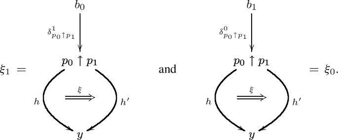
• 2. For every pair of 2-cells

  $$\begin{aligned} (\xi _ 0: h\cdot \delta _{p_0\uparrow {p_1}}^0\Rightarrow h'\cdot \delta _{p_0\uparrow {p_1}}^0: b_1\rightarrow y,\quad \xi _ 1: h\cdot \delta _{p_0\uparrow {p_1}}^1\Rightarrow h'\cdot \delta _{p_0\uparrow {p_1}}^1: b_0\rightarrow y ) \end{aligned}$$

  such that

  

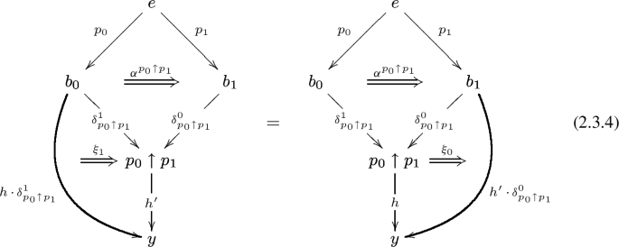
  holds, there is a unique 2-cell $\xi : h\Rightarrow h': p_0\uparrow p_1\rightarrow y$ such that

  

Remark 2.4

Since ${\textsf {Cat}}$ has all weighted colimits and limits, it has opcomma objects. More generally, if any 2-category ${\mathbb {A}}$ has tensorial coproducts and pushouts, then ${\mathbb {A}}$ has opcomma objects.

More precisely, assuming that the tensorial coproduct $\textsf {2}\otimes e$ exists in ${\mathbb {A}}$, we have the universal 2-cell $d^1\otimes e\Rightarrow d^0\otimes e: e\rightarrow \textsf {2}\otimes e$ given by the image of the identity $\textsf {2}\otimes e\rightarrow \textsf {2}\otimes e$ by the isomorphism

$$\begin{aligned} {\mathbb {A}}(\textsf {2}\otimes e, \textsf {2}\otimes e )\cong {\textsf {Cat}}\left[ \textsf {2}, {\mathbb {A}}(e, \textsf {2}\otimes e) \right] . \end{aligned}$$

If it exists, the conical colimit of the diagram below is the opcomma object $p_0\uparrow p_1$ of $p_1: e\rightarrow b_1$ along $p_0: e\rightarrow b_0$.

3.4 Lax Descent Objects

We consider the 2-category $\Delta _ \text {Str}$ of Definition 1.1 and we define the weight $\mathfrak {D}: \Delta _ \text {Str}\rightarrow {\textsf {Cat}}$ by

in which:

• The functor $\overline{S}: \Delta _ \text {Str}({\underline{\textsf {1} } },{\underline{\textsf {1} } })\times \textsf {2}\rightarrow \Delta _ \text {Str}({\underline{\textsf {1} } },{\underline{\textsf {1} } })\times \textsf {1}$ is defined by

  $$\begin{aligned} \overline{S} (\overline{v}: v\cong v', \textsf {0}\rightarrow \textsf {1} ) = \left( \left( \mathfrak {n}_0^{-1}\cdot \mathfrak {n}_1 \right) *\overline{v}, \textrm{id}_ {\textsf {0}}\right) = \left( s^0 d ^1 v\cong s^0 d^0 v', \textrm{id}_ {\textsf {0}}\right) . \end{aligned}$$

• $\left\langle \textsf {3}\right\rangle$ is the category corresponding to the preordered set

  $$\begin{aligned} \left\{ (\textsf {i}, \textsf {k} )\in \left\{ \textsf {0}, \textsf {1}, \textsf {2}\right\} ^2: \textsf {i}\ne \textsf {k}\right\} \end{aligned}$$

  in which the preorder induced by the first coordinate, that is to say, $(\textsf {i}, \textsf {k})\le (\textsf {i}', \textsf {k}')$ if $\textsf {i}\le \textsf {i}'$. In other words, the category $\left\langle \textsf {3}\right\rangle$ is defined by the preordered set below.

  

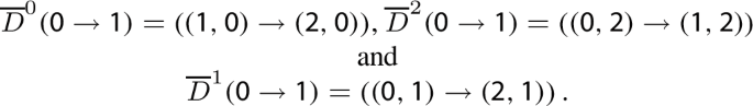
• The functors $\overline{D}^0, \overline{D}^1, \overline{D}^2: \textsf {2}\rightarrow \left\langle \textsf {3}\right\rangle$ are defined by

  

• The natural transformations $\mathfrak {D} (\sigma _ {01} )$, $\mathfrak {D} (\sigma _ {02} )$ and $\mathfrak {D} (\sigma _ {12} )$ are defined by

  $$\begin{aligned} \mathfrak {D} (\sigma _ {ij} ):= \textrm{id}_ {\textrm{id}_ {\Delta _ \text {Str}({\underline{\textsf {1} } },{\underline{\textsf {1} } })}}\times \overline{\mathfrak {D} (\sigma _ {ij} )}, \end{aligned}$$

  in which

  

• The natural transformation

  $$\begin{aligned} \mathfrak {D} (\mathfrak {n} _ {i} ): \overline{S}\circ \left( \textrm{id}_ {\Delta _ \text {Str}({\underline{\textsf {1} } }, {\underline{\textsf {1} } })}\times d^i\right) \Rightarrow \textrm{id}_ {\Delta _ \text {Str}({\underline{\textsf {1} } }, {\underline{\textsf {1} } })\times \textsf {1} } \end{aligned}$$

  is defined by $\mathfrak {D} (\mathfrak {n} _ {i} )_{ (v, \textsf {0} ) }: = \left( \mathfrak {n} _ {i}*\textrm{id}_ v, \textrm{id}_{\textsf {0}} \right)$.

Definition 2.6

(Lax descent object) Given a 2-functor $\mathcal {B}: \Delta _ {\text {Str}}\rightarrow {\mathbb {A}}$, if it exists, the weighted limit $\mathrm{\mathsf lim}(\mathfrak {D}, \mathcal {B})$ is called the lax descent object of $\mathcal {B}$.

Remark 2.7

Since ${\textsf {Cat}}$ has all weighted limits, it has lax descent objects. More precisely, if $\mathcal {A}: \Delta _ {\text {Str}}\rightarrow {\textsf {Cat}}$ is a 2-functor,

$$\begin{aligned} \mathrm{\mathsf lim}(\mathfrak {D}, \mathcal {A})\cong \left[ \Delta _ {\text {Str}}, {\textsf {Cat}}\right] (\mathfrak {D}, \mathcal {A}) \end{aligned}$$

is the category in which:

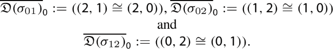
• 1. Objects are 2-natural transformations ${\overline{\psi }}: \mathfrak {D} \longrightarrow \mathcal {A}$. We have a bijective correspondence between such 2-natural transformations and pairs $(w, \psi )$ in which w is an object of $\mathcal {A}({\underline{\textsf {1} } })$ and is a morphism in $\mathcal {A}({\underline{\textsf {2} } })$ satisfying the following equations:

  • Associativity:

    $$\begin{aligned} \mathcal {A}(\mathbbm {d}^0 )(\psi )\,\cdot \, \mathcal {A}(\sigma _ {02}) _ {w}\, \cdot \, \mathcal {A}(\mathbbm {d}^2)(\psi ) = \mathcal {A}(\sigma _ {01} )_ {w}\,\cdot \,\mathcal {A}(\mathbbm {d}^1)(\psi )\,\cdot \,\mathcal {A}(\sigma _ {12}) _ {w}; \end{aligned}$$

  • Identity:

    

  If ${\overline{\psi }}: \mathfrak {D}\longrightarrow \mathcal {A}$ is a 2-natural transformation, we get such pair by the correspondence

  $$\begin{aligned} {\overline{\psi }} \mapsto ({\overline{\psi }}_{{\underline{\textsf {1} } }} (\textrm{id}_ {{}_{{\underline{\textsf {1} } }}}, \textsf {0} ), {\overline{\psi }} _ {{\underline{\textsf {2} } }} (\textrm{id}_ {{}_{{\underline{\textsf {1} } }}}, \textsf {0}\rightarrow \textsf {1} ) ). \end{aligned}$$

• 2. The morphisms are modifications. In other words, a morphism $\mathfrak {m}: (w, \psi )\rightarrow (w', \psi ')$ is determined by a morphism $\mathfrak {m}: w\rightarrow w'$ in $\mathcal {A}({\underline{\textsf {1} } })$ such that

  

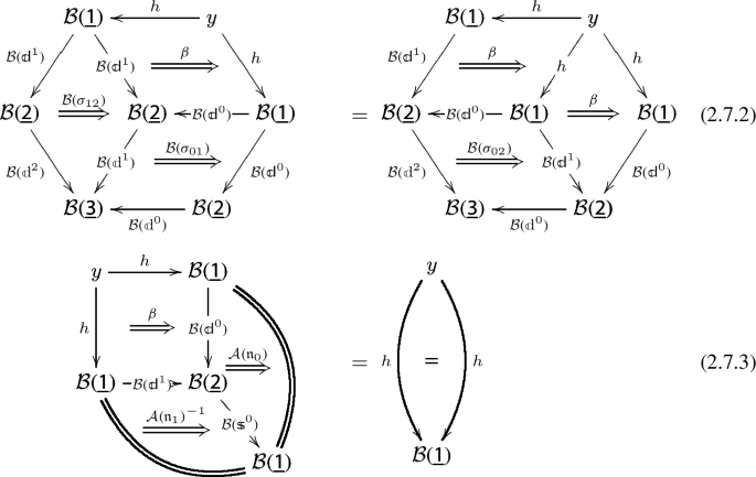
By definition, if $\mathcal {B}: \Delta _ {\text {Str}}\rightarrow {\mathbb {A}}$ is a 2-functor, an object $\text {lax}\text {-}\mathcal {D}\text {esc}\left( \mathcal {B}\right)$ is the lax descent object $\mathrm{\mathsf lim}(\mathfrak {D}, \mathcal {B})$ of $\mathcal {B}$ if and only if there is a 2-natural isomorphism (in y)

$$\begin{aligned} {\mathbb {A}}(y, \text {lax}\text {-}\mathcal {D}\text {esc}\left( \mathcal {B}\right) )\cong \mathrm{\mathsf lim}(\mathfrak {D}, {\mathbb {A}}(y, \mathcal {B}-) ). \end{aligned}$$

Equivalently, a lax descent object of $\mathcal {B}$ is, if it exists, an object $\mathrm{\mathsf lim}(\mathfrak {D},\mathcal {B})$ of ${\mathbb {A}}$ together with a pair

of a morphism and a 2-cell $\Psi ^{\left( \mathfrak {D},\mathcal {B}\right) }$ in ${\mathbb {A}}$ satisfying the following three properties.

• 1. For each pair

  

  in which h is a morphism and $\beta$ is a 2-cell of ${\mathbb {A}}$ such that the equations

  

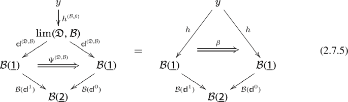
  hold, there is a unique morphism $h^{( \mathcal {B}, \beta ) }: y\rightarrow \mathrm{\mathsf lim}(\mathfrak {D}, \mathcal {B})$ making the diagram

  

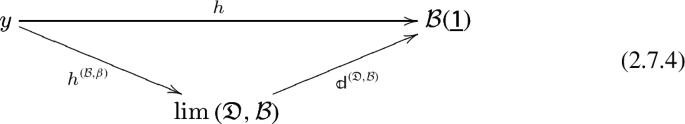
  commutative and such that (2.7.5) holds.

  

• 2. The pair satisfies the descent associativity (2.7.2) and the descent identity (2.7.3). In this case, the unique morphism induced is clearly the identity on $\mathrm{\mathsf lim}(\mathfrak {D}, \mathcal {B})$, that is to say,

  

• 3. Assume that $(h _ 1, \beta _1 )$ and $(h_0, \beta _ 0 )$ are pairs satisfying (2.7.2) and (2.7.3), inducing factorizations and .

  For each 2-cell

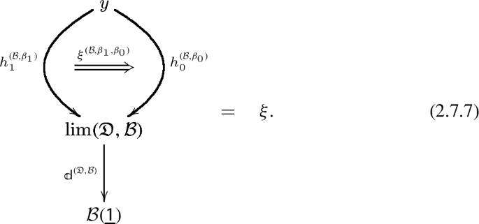
  $$\begin{aligned} \xi : h_1\Rightarrow h_0: y\rightarrow \mathcal {B}({\underline{\textsf {1} } }) \end{aligned}$$

  satisfying the equation

  

  there is a unique 2-cell

  $$\begin{aligned} \xi ^{(\mathcal {B}, \beta _ 1, \beta _0)}: h_1 ^{(\mathcal {B}, \beta _1)}\Rightarrow h _0^{(\mathcal {B}, \beta _ 0 )}: y\rightarrow \mathrm{\mathsf lim}(\mathfrak {D}, \mathcal {B}) \end{aligned}$$

  such that

  

3.5 The Two-Dimensional Cokernel Diagram

Let $p: e\rightarrow b$ be a morphism of a 2-category ${\mathbb {A}}$. ${\mathbb {A}}$ has the two-dimensional cokernel diagram of p if ${\mathbb {A}}$ has the opcomma object

of p along itself and the pushout (2.8.2) of $\delta ^0$ along $\delta ^1$.

Henceforth, in this section, we assume that ${\mathbb {A}}$ has the two-dimensional cokernel diagram of p. We denote by

$$\begin{aligned} \partial ^1: b\uparrow _p b\rightarrow b\uparrow _p b \uparrow _p b \end{aligned}$$

the unique morphism such that the equations

$$\begin{aligned} \partial ^1 \, \delta ^1 = \partial ^2\, \delta ^1 ,\quad \partial ^1 \, \delta ^0 = \partial ^0\, \delta ^0 \end{aligned}$$

(2.8.3)

hold, while we denote by ${\mathfrak {s}}^0:b\uparrow _ p b\rightarrow b$ the unique morphism such that ${\mathfrak {s}}^0\cdot \delta ^1 = {\mathfrak {s}}^0 \cdot \delta ^0 = \textrm{id}_ b$ and (2.8.5) holds.

Definition 2.9

(Two-dimensional cokernel diagram) Consider the 2-functor

$$\begin{aligned} \mathcal {H}_p ': \Delta _\text {3}\rightarrow {\mathbb {A}}\end{aligned}$$

defined by $\mathcal {H}_p ' (d^i: \textsf {1}\rightarrow \textsf {2} ) = \delta ^i$, $\mathcal {H}_p ' (d^i: \textsf {2}\rightarrow \textsf {3} ) = \partial ^i$ and $\mathcal {H}_p ' (s ^0) = {\mathfrak {s}}^0$. The 2-functor

$$\begin{aligned} \mathcal {H}_p: = \mathcal {H}_p '\circ \texttt {e}_{\Delta _ \text {Str} }: \Delta _\text {Str}\rightarrow {\mathbb {A}}\end{aligned}$$

is called the two-dimensional cokernel diagram of p.

Remark 2.10

This construction was, for instance, already considered in [31, pag. 135] under the name resolution, specially in the 2-category of pretoposes and in the 2-category of exact categories.

Remark 2.11

The 2-category of categories ${\textsf {Cat}}$ has the two-dimensional cokernel diagram of any functor. In particular, the two-dimensional cokernel diagram of $\textrm{id}_ \textsf {1}$ is

which is just the usual inclusion of the locally discrete 2-category $\Delta _ \text {3}$ in ${\textsf {Cat}}$.

By the definitions of $\partial ^1$ and ${\mathfrak {s}}^0$ ((2.8.4) and (2.8.5)), the pair

$$\begin{aligned} (p: e\rightarrow b,\quad \upalpha : \delta ^1 \cdot p\Rightarrow \delta ^0 \cdot p: e \rightarrow b\uparrow _ p b ) \end{aligned}$$

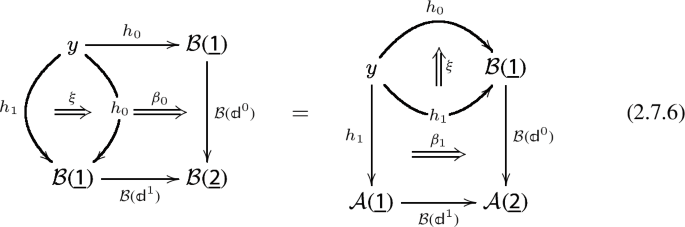
satisfies the descent associativity and identity w.r.t. $\mathcal {H}_p: \Delta _\text {Str}\rightarrow {\mathbb {A}}$ (that is to say, (2.7.2) and (2.7.3) w.r.t. $\mathcal {H}_p$). Hence, if ${\mathbb {A}}$ has the lax descent object

of $\mathcal {H}_p$, by the universal property of the lax descent object, there is a unique morphism

$$\begin{aligned} p^\mathcal {H}:= p ^{(\mathcal {H}_p, \upalpha )}: e\rightarrow \mathrm{\mathsf lim}(\mathfrak {D}, \mathcal {H}_p) \end{aligned}$$

such that

commutes and the equation

holds.

Inspired by our main result (Theorem 4.7), we establish the following terminology.

Definition 2.12

Assume that ${\mathbb {A}}$ has the lax descent object of $\mathcal {H}_p$. The lax descent factorization induced by $\mathcal {H}_p$ and the universal 2-cell of the opcomma object $b\uparrow _pb$ given in (2.11.1) is called the semantic lax descent factorization of p.

Remark 2.13

Given an object x and a morphism $p: e\rightarrow b$ of ${\mathbb {A}}$ as above, the factorization induced by the universal property of the lax descent category $\mathrm{\mathsf lim}(\mathfrak {D}, {\mathbb {A}}(x,\mathcal {H}_p -) )$ and by the pair

is given by

in which

Clearly, if ${\mathbb {A}}$ has the lax descent object of the two-dimensional cokernel diagram $\mathcal {H}_p$, the factorization given in (2.13.2) is isomorphic to the factorization

(2.13.3)

given by the image of (2.11.1) by ${\mathbb {A}}(x,-): {\mathbb {A}}\rightarrow {\textsf {Cat}}$, since the Yoneda embedding creates any existing lax descent objects in ${\mathbb {A}}$.

Remark 2.14

It should be noted that, assuming that we can construct $\mathcal {H}_ p$ in ${\mathbb {A}}$, the factorization (2.13.2) always exists, since ${\textsf {Cat}}$ has lax descent objects (lax descent categories).

Moreover, since opcomma objects (weighted colimits in general) might not be preserved by the Yoneda embedding, the definition of the factorization given in (2.13.2) does not coincide with the definition of semantic lax descent factorization of ${\mathbb {A}}(x, p )$ in ${\textsf {Cat}}$.

For instance, consider the example of Remark 2.11. For any object x of ${\textsf {Cat}}$, clearly the opcomma object of ${\textsf {Cat}}[x, \textrm{id}_ {\textsf {1}}]$ along itself is isomorphic to the opcomma object of $\textrm{id}_ {\textsf {1}}$ along itself, that is to say, $\textsf {2}$. Hence, since there is a category x such that ${\textsf {Cat}}[x, \textsf {2} ]$ is not isomorphic to $\textsf {2}$, this shows that the Yoneda embedding does not preserve the opcomma object $\textrm{id}_ {\textsf {1}}\uparrow \textrm{id}_ {\textsf {1}}$.

Remark 2.15

(Duality: two-dimensional kernel diagram and the induced factorization) The codual notion of that of the two-dimensional cokernel diagram gives the same notion of factorization (assuming the existence of the suitable lax descent object): namely, the factorization given in (2.11.1) of the morphism p.

The dual concept of the two-dimensional cokernel diagram, the 2-dimensional kernel diagram of $l:b\rightarrow e$, if it exists, is a 2-functor

$$\begin{aligned} \mathcal {H}^l: \Delta _{\text {Str}} ^{\textrm{op}}\rightarrow {\mathbb {A}}\end{aligned}$$

constructed from suitable comma objects and pullbacks.

In this case, we get the lax codescent factorization induced by the 2-dimensional kernel diagram of l (2.15.1), provided that the lax codescent object of $\mathcal {H}^l$ exists. Herein, we call the factorization (2.15.1) the semantic lax codescent factorization of l.

In the special case of the 2-category ${\textsf {Cat}}$, the 2-dimensional kernel diagram was, for instance, also considered in [29, pag. 544] under the name higher kernel and at [14, Proposition 4.7] under the name congruence.

4 Semantic Factorization

Assuming that ${\mathbb {A}}$ has suitable Eilenberg–Moore objects, the semantics-structure adjunction (e.g. [25, Section 2]) gives rise to what is called herein the semantic factorization of a tractable morphism p. In this section, we recall the semantic factorization of morphisms that have codensity monads. Before doing so, we recall the definition of the Eilenberg–Moore object of a given monad.

4.1 Eilenberg–Moore Object

Recall that a monad in a 2-category ${\mathbb {A}}$ is a quadruple

in which b is an object, t is a morphism and $m, \eta$ are 2-cells in ${\mathbb {A}}$ such that the equations

hold. A monad can be seen as a 2-functor $\texttt {t} : \mathrm{\mathsf mnd}\rightarrow {\mathbb {A}}$ from the free monad 2-category $\mathrm{\mathsf mnd}= \Sigma \Delta$ to ${\mathbb {A}}$ (e.g. [28, pag. 178] or [19, Sect. 6]). If it exists, the Eilenberg–Moore object, also called the object of algebras, is a special weighted limit of $\texttt {t}$. More precisely, given a monad $\texttt {t}$ in ${\mathbb {A}}$, the object $b^\texttt {t}$ is the Eilenberg–Moore object of $\texttt {t}$ if and only if there is a 2-natural isomorphism (in y)

$$\begin{aligned} {\mathbb {A}}( y, b ^\texttt {t} )\cong {\mathbb {A}}(y, b) ^{{\mathbb {A}}(y, \texttt {t} )} \end{aligned}$$

in which ${\mathbb {A}}(y, b) ^{{\mathbb {A}}(y, \texttt {t} )}$ is the Eilenberg–Moore category of the monad

$$\begin{aligned} ({\mathbb {A}}(y, b ), {\mathbb {A}}(y, t ), {\mathbb {A}}(y, m ), {\mathbb {A}}(y, \eta )) \end{aligned}$$

in ${\textsf {Cat}}$. This means that, if the Eilenberg–Moore object $b ^\texttt {t}$ of $\texttt {t} = (b, t, m, \eta )$ exists, it is characterized by the following universal property. There is a pair

in which is a morphism, and $\mu ^\texttt {t}$ is a 2-cell in ${\mathbb {A}}$ satisfying the following three properties.

• 1. For each pair $( h: y\rightarrow b, \beta : t\cdot h\Rightarrow h )$ in which h is a morphism and $\beta$ is a 2-cell in ${\mathbb {A}}$ making the equations

  

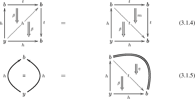
  hold, there is a unique morphism $h^{( \texttt {t} , \beta ) }: y\rightarrow b ^\texttt {t}$ such that the equation $\mu ^\texttt {t} *\textrm{id}_{h^{( \texttt {t} , \beta ) }} = \beta$. It should be noted that, in this case, we get in particular that

  

  commutes.

• 2. The pair satisfies the algebra associativity (3.1.4) and identity (3.1.5) equations. In this case, the unique morphism induced is clearly the identity on $b ^\texttt {t}$.

• 3. Assume that $h_1 ^{(\texttt {t} , \beta _1 )}, h _0^{(\texttt {t} , \beta _0 )}: y\rightarrow b ^\texttt {t}$ are morphisms in ${\mathbb {A}}$. For each 2-cell

  

  such that the equation

  

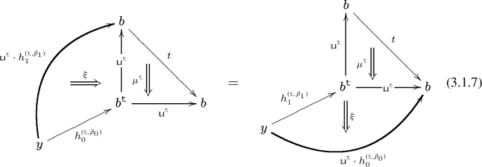
  is satisfied, there is a unique 2-cell

  $$\begin{aligned} \xi _{(\texttt {t} , \beta _1, \beta _0)}: h_1^{(\texttt {t} , \beta _1 )}\Rightarrow h _0^{(\texttt {t} , \beta _0 )}: y\rightarrow b ^\texttt {t} \end{aligned}$$

  such that

  

Remark 3.2

(Duality: Kleisli objects and co-Eilenberg–Moore objects) The dual of the notion of Eilenberg–Moore object of a monad is called the Kleisli object of a monad, while the codual is called the co-Eilenberg–Moore object, or object of coalgebras, of a comonad. In the special case of ${\textsf {Cat}}$, these notions coincide with the usual ones (e.g. [25, Section 5]).

4.2 Kan Extensions

Let $f: z\rightarrow y$ and $g: z\rightarrow x$ be morphisms of a 2-category ${\mathbb {A}}$. The right Kan extension of f along g is, if it exists, the right reflection $\textrm{ran}_ g f$ of f along the functor

$$\begin{aligned} {\mathbb {A}}(g, y ): {\mathbb {A}}(x, y)\rightarrow {\mathbb {A}}(z, y). \end{aligned}$$

This means that the right Kan extension is actually a pair

$$\begin{aligned} \left( \textrm{ran}_ g f: x\rightarrow y, \gamma ^{ \textrm{ran}_ g f }: \left( \textrm{ran}_ g f\right) \cdot g\Rightarrow f \right) \end{aligned}$$

of a morphism $\textrm{ran}_ g f$ and a 2-cell $\gamma ^{ \textrm{ran}_ g f }$, called the universal 2-cell, such that, for each morphism $h: x\rightarrow y$ of ${\mathbb {A}}$,

defines a bijection ${\mathbb {A}}(x,y)(h, \textrm{ran}_ g f)\cong {\mathbb {A}}(z,y)(h \cdot g, f)$.

Remark 3.4

(Duality: right lifting and left Kan extension) The dual notion of that of a right Kan extension is called right lifting (see [30, Section 1]), while the codual notion is called the left Kan extension. Finally, of course, we also have the codual notion of the right lifting: the left lifting.

Let $p_0: e\rightarrow b_0, p_1: e\rightarrow b_1$ be morphisms of a 2-category ${\mathbb {A}}$. Assume that ${\mathbb {A}}$ has the opcomma object $p_0\uparrow p_1$ and

$$\begin{aligned} \alpha ^{p_0\uparrow p_1}: \delta ^1 _{p_0\uparrow p_1 }\cdot p_0\Rightarrow \delta ^0 _{p_0\uparrow p_1 }\cdot p_1 \end{aligned}$$

is the universal 2-cell that gives $p_0\uparrow p_1$ as the opcomma object of $p_1$ along $p_0$, as in 2.3 (Eq. 2.3.2). In this case, we have:

Lemma 3.5

Given a morphism $h: p_0\uparrow p_1\rightarrow y$, the following statements are equivalent.

• (i) The pair $(h,\, \textrm{id}_ { h\cdot \delta ^0_{p_0\uparrow p_1}} )$ is the right Kan extension of $h\cdot \delta ^0_{p_0\uparrow p_1}$ along $\delta ^0_{p_0\uparrow p_1}$.

• (ii) The pair $(h\cdot \delta ^1_{p_0\uparrow p_1},\, \textrm{id}_ h *\alpha ^{p_0\uparrow p_1} )$ is the right Kan extension of $h\cdot \delta ^0_{p_0\uparrow p_1}\cdot p_1$ along $p_0$.

Proof

Assuming i), given a 2-cell

$$\begin{aligned} \check{\beta }: h'_1 \cdot p_0\Rightarrow h\cdot \delta ^0_{p_0\uparrow p_1}\cdot p_1: e\rightarrow y, \end{aligned}$$

we conclude, by the universal property of the opcomma object, that there is a unique morphism $h': p_0\uparrow p_1\rightarrow y$ such that

and $h' \cdot \delta ^0_{p_0\uparrow p_1} = h\cdot \delta ^0_{p_0\uparrow p_1}$.

By the universal property of the Kan extension, there is a unique 2-cell $\underline{\beta }: h'\Rightarrow h$ such that the equation

is satisfied.

By the universal property of the opcomma object (see (2.3.4)), this means that $\underline{\beta }*\textrm{id}_ {\delta ^1_{p_0\uparrow p_1}}$ is the unique 2-cell such that

This proves ii).

Reciprocally, assuming ii), by the universal property of the right Kan extension

$$\begin{aligned} \textrm{ran}_{p_0} \left( h\cdot \delta ^0 _{p_0\uparrow p_1}\cdot p_1\right) = (h\cdot \delta ^1_{p_0\uparrow p_1},\, \textrm{id}_ h *\alpha ^{p_0\uparrow p_1} ) \end{aligned}$$

of the hypothesis, we have that, given any 2-cell

$$\begin{aligned} \beta _0: h'\cdot \delta ^0 _{p_0\uparrow p_1}\Rightarrow h\cdot \delta ^0 _{p_0\uparrow p_1}, \end{aligned}$$

there is a unique 2-cell $\beta _1: h'\cdot \delta ^1 _{p_0\uparrow p_1}\Rightarrow h\cdot \delta ^1 _{p_0\uparrow p_1}$ such that

holds, in which, for each $i\in \left\{ 1,2 \right\}$, $h_i ': = h ' \cdot \delta ^i _{p_0\uparrow p_1}$ and $h_i: = h \cdot \delta ^i _{p_0\uparrow p_1}$.

By the universal property of the opcomma $p_0\uparrow p_1$, this implies that there is a unique $\beta : h'\Rightarrow h$ such that $\beta *\textrm{id}_ {\delta ^0 _{p_0\uparrow p_1} } = \beta _0$. Hence we get i). $\square$

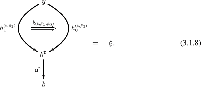
Definition 3.6

(Codensity monad) A morphism $p: e\rightarrow b$ of a 2-category ${\mathbb {A}}$ has the codensity monad if the right Kan extension $( \textrm{ran}_p p, \gamma )$ of p along itself exists. Assuming that ${\mathbb {A}}$ has the codensity monad of p and denoting $\textrm{ran}_p p$ by t, we consider:

• the 2-cell $m: t^2\Rightarrow t$ such that

  

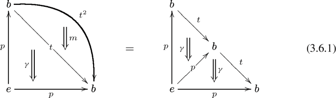
  holds;

• the 2-cell $\eta : \textrm{id}_ b\Rightarrow t$ such that (3.6.2) holds.

  

In this case, by the universal property of the right Kan extension of p along itself, the quadruple $\texttt {t} = (b, t, m, \eta )$ is a monad called the codensity monad of p.

Assuming that $\texttt {t} = (b, t, m, \eta )$ is the codensity monad of $p: e\rightarrow b$ as above, by (3.6.1) and (3.6.2), it is clear that the pair $(p: e\rightarrow b,\, \gamma : t\cdot p\Rightarrow p )$ satisfies the algebra associativity and identity equations w.r.t. the monad $\texttt {t}$ (that is to say, (3.1.5) and (3.1.4) w.r.t. the monad $\texttt {t}$). Hence, assuming that ${\mathbb {A}}$ has the Eilenberg–Moore object of the monad $\texttt {t}$, by the universal property, there is a unique $p^\texttt {t} := p^{(\texttt {t} , \gamma )}$ such that

commutes and $\mu ^\texttt {t} *\textrm{id}_ {p ^\texttt {t} } = \gamma$.

Definition 3.7

The factorization given by (3.6.3) is called herein the semantic factorization of p.

For each object x, assuming the existence of the semantic factorization of p, we can take its image by the representable 2-functor ${\mathbb {A}}(x, -): {\mathbb {A}}\rightarrow {\textsf {Cat}}$, getting the factorization

(3.7.1)

Since the Yoneda embedding creates any existing Eilenberg–Moore object of ${\mathbb {A}}$, the factorization (3.7.1) coincides up to isomorphism with the factorization of ${\mathbb {A}}(x, p )$ induced by $\left( {\mathbb {A}}(x, p ),{\mathbb {A}}(x, \gamma )\right)$ and ${\mathbb {A}}(x, b) ^{{\mathbb {A}}(x, \texttt {t} ) }$; that is to say, the commutative triangle

which is given by

Remark 3.8

Let p be a morphism of ${\mathbb {A}}$ which has the codensity monad $\texttt {t}$. Since ${\textsf {Cat}}$ has Eilenberg–Moore objects, the factorization of ${\mathbb {A}}(x, p )$ induced by $\left( {\mathbb {A}}(x, p ),{\mathbb {A}}(x, \gamma )\right)$ and ${\mathbb {A}}(x, b) ^{{\mathbb {A}}(x, \texttt {t} ) }$ as above always exists, even if ${\mathbb {A}}$ does not have the Eilenberg–Moore object of $\texttt {t}$.

Remark 3.9

(Duality: op-codensity monad) The codual notion of the notion of codensity monad is that of density comonad, which is induced by the left Kan extension of the morphism along itself, assuming its existence.

The dual notion is herein called op-codensity monad. Notice that, if it exists, the op-codensity monad of a morphism is induced by the right lifting of the morphism through itself. Finally, of course, we have also the codual notion of the op-codensity monad, called herein the op-density comonad.

Therefore, we also have factorizations: assuming the existence of the Kleisli object of the op-codensity monad of a morphism, we get the op-semantic factorization. Codually, we have the co-semantic factorization of a morphism that has the density comonad, provided that the 2-category has its co-Eilenberg–Moore object.

4.3 Right Adjoint Morphism

Recall that an adjunction inside a 2-category ${\mathbb {A}}$ is a quadruple

$$\begin{aligned} \left( l: b\rightarrow e,\, p:e\rightarrow b,\, \varepsilon : lp\Rightarrow \textrm{id}_ e,\, \eta : \textrm{id}_ b\Rightarrow pl \right) \end{aligned}$$

in which l, p are 1-cells and $\varepsilon , \eta$ are 2-cells of ${\mathbb {A}}$ satisfying the triangle identities. This means that

are, respectively, the identities $\textrm{id}_ l: l\Rightarrow l$ and $\textrm{id}_ p: p\Rightarrow p$. In this case, p is right adjoint to l and we denote the adjunction by $( l\dashv p, \varepsilon , \eta ): b\rightarrow e$.

If $(l\dashv p,\varepsilon , \eta ): b\rightarrow e$ is an adjunction in a 2-category ${\mathbb {A}}$, p has the codensity monad and the op-density comonad. More precisely, in this case, the pair $(pl, \textrm{id}_p *\varepsilon )$ is the right Kan extension of p along itself and $(lp, \eta *\textrm{id}_ p )$ is the left lifting of p through itself. Hence, the codensity monad of p coincides with the monad $\texttt {t} = (b, pl, \textrm{id}_ p *\varepsilon *\textrm{id}_ l, \eta )$ induced by the adjunction, while the op-density comonad coincides with the comonad $(e, lp, \textrm{id}_ l *\eta *\textrm{id}_ p, \varepsilon )$ induced by the adjunction. Codually, if $(l\dashv p,\varepsilon , \eta ): b\rightarrow e$ is an adjunction, the density comonad and the op-codensity monad induced by $l: b\rightarrow e$ are the same of those induced by the adjunction.

Assuming the existence of the Eilenberg–Moore object of the monad (codensity monad $\texttt {t}$) induced by the adjunction $(l\dashv p,\varepsilon , \eta )$, the semantic factorization is the usual factorization of the right adjoint morphism through the object of algebras. Dually and codually, assuming the existence of the suitable weighted limits and colimits, we get all the four usual factorizations of l and p.

More precisely, the op-semantic factorization of $l: b\rightarrow e$ is the usual Kleisli factorization

w.r.t. the induced monad ${(b, pl, \textrm{id}_ p *\varepsilon *\textrm{id}_ l, \eta )}$. Codually and dually, the co-semantic and the coop-semantic factorizations are, respectively, the usual factorization of l through the co-Eilenberg–Moore object, and the usual factorization of p through the co-Kleisli object of the comonad $(e, lp, \textrm{id}_ l *\eta *\textrm{id}_ p, \varepsilon )$.

Definition 3.11

(Preservation of a Kan extension) Let $\left( \textrm{ran}_ g f, \gamma ^{ \textrm{ran}_ g f } \right)$ be the right Kan extension of $f: z\rightarrow y$ along g in a 2-category ${\mathbb {A}}$. A morphism $\delta : y\rightarrow y '$ preserves the right Kan extension $\textrm{ran}_ g f$ if

gives the right Kan extension of the morphism $\delta \cdot f$ along g. Furthermore, the right Kan extension $\left( \textrm{ran}_ g f, \gamma ^{ \textrm{ran}_ g f } \right)$ is absolute if it is preserved by any morphism with domain in y.

Remark 3.12

(Duality: respecting liftings) The dual notion of that of preservation of a Kan extension is that of respecting a lifting. If a pair $\left( \textrm{rlift}_ g f, \upgamma ^{ \textrm{rlift}_ g f } \right)$ is the right lifting of f through g, a morphism $\delta : y'\rightarrow y$ respects the right lifting of f through g if $\left( \left( \textrm{rlift}_ g f\right) \cdot \delta , \upgamma ^{ \textrm{rlift}_ g f }*\textrm{id}_ \delta \right)$ is the right lifting of $f\cdot \delta$ through g.

Remark 3.13

In some contexts, such as in the case of 2-categories endowed with Yoneda structures [30], we have a stronger notion of Kan extensions: the pointwise Kan extensions (for instance, see [5, Theorem I.4.3] for the case of the 2-category of V-enriched categories). Although this concept plays a fundamental role in the theory of Kan extensions, we do not use this notion in our main theorem. However, we mention them in our examples and, herein, a pointwise Kan extension of a functor in ${\textsf {Cat}}$ is just a Kan extension that is preserved by any representable functor. See [22, Section X.5] for basic aspects of pointwise Kan extensions and their constructions via conical (co)limits.

If $(l\dashv p,\varepsilon , \eta ): b\rightarrow e$ is an adjunction in a 2-category ${\mathbb {A}}$, p preserves any right Kan extension with codomain in b. Furthermore:

Theorem 3.14

(Dubuc-Street [5, 30]) If $p:e\rightarrow b$ is a morphism in a 2-category ${\mathbb {A}}$, the following statements are equivalent.

• (i) The pair $(l, \varepsilon )$ is the right Kan extension of $\textrm{id}_ e$ along p and it is preserved by p.

• (ii) The pair $(l, \varepsilon )$ is the right Kan extension of $\textrm{id}_ e$ along p and it is absolute.

• (iii) The morphism p has a left adjoint l, with the counit $\varepsilon : lp\Rightarrow \textrm{id}_ e$.

In particular, if $p: e\rightarrow b$ has a left adjoint, then it has the codensity monad and the right Kan extension of p along itself is absolute.

Proof

See [5, Theorem I.4.1] or [30, Propositions 2]. $\square$

Remark 3.15

(Mate correspondence) Assume that

$$\begin{aligned} (l_1\dashv p_1):= (l_1\dashv p_1, \varepsilon _1, \eta _1 ): b_1\rightarrow e_1 \hbox { and }(l_0\dashv p_0):= (l_0\dashv p_0, \varepsilon _0, \eta _ 0 ): b_0\rightarrow e_0 \end{aligned}$$

in a 2-category ${\mathbb {A}}$. Recall that we have the mate correspondence [12, Proposition 2.1]. More precisely, given 1-cells $h_b: b_0\rightarrow b_1$ and $h_e: e_0\rightarrow e_1$ of ${\mathbb {A}}$, there is a bijection

$$\begin{aligned} {\mathbb {A}}(e_0,b_1)\left( h_b\cdot p_ 0,\, p_1\cdot h_e\right) \cong {\mathbb {A}}(b_0,e_1)\left( l_1\cdot h_b,\, h_e\cdot l_ 0 \right) \end{aligned}$$

defined by

whose inverse is given by

The image of a 2-cell $\beta : h_b\cdot p_ 0 \Rightarrow p_1\cdot h_e$ by the isomorphism ${\mathbb {A}}(e_0,b_1)(h_b\cdot p_ 0, p_1\cdot h_e)\cong {\mathbb {A}}(b_0,e_1)( l_1\cdot h_b, h_e\cdot l_ 0 )$ above is called the mate of $\beta$ under the adjunction $l_0\dashv p_0$ and $l_1\dashv p_1$.

5 Main Theorems

Let ${\mathbb {A}}$ be a 2-category and $p: e\rightarrow b$ a morphism of ${\mathbb {A}}$. Throughout this section, we assume that p has the codensity monad $\texttt {t} = (b, t, m, \eta )$, in which $\left( t, \gamma \right)$ is the right Kan extension of p along itself. Furthermore, we assume that ${\mathbb {A}}$ has the two-dimensional cokernel diagram $\mathcal {H}_ p:\Delta _\text {Str} \rightarrow {\mathbb {A}}$ of p.

We follow the notation respectively established in3.6, 2.8and2.9for the codensity monad of p, the two-dimensional cokernel diagram of p and the morphisms involved in the diagram.

Moreover, by the universal property of the opcomma object $b\uparrow _ p b$, there is a unique morphism $\ell$ such that (4.0.1) and (4.0.2) hold. Henceforth, we denoted this morphism by $\ell : b\uparrow _ p b\rightarrow b$.

$$\begin{aligned} \ell \cdot \delta ^0 = \textrm{id}_ b, \quad \ell \cdot \delta ^1 = t, \end{aligned}$$

(4.0.1)

Proposition 4.1

The pair $(\ell , \textrm{id}_ {\textrm{id}_ {b} } )$ is the right Kan extension of $\textrm{id}_{b}$ along $\delta ^0: b\rightarrow b\uparrow _ p b$.

Proof

By Lemma 3.5, since $(t, \gamma )$ is the right Kan extension of $\ell \cdot \delta ^0\cdot p=p$ along p, we get that $(\ell , \gamma )$ is the right Kan extension of $\ell \cdot \delta ^0 = \textrm{id}_ b$ along $\delta ^0$. $\square$

Proposition 4.2

(Condition) The right Kan extension $(t, \gamma )$ of p along itself is preserved by $\delta ^0: b\rightarrow b\uparrow _ p b$ if and only if $\ell$ is left adjoint to $\delta ^0$. In this case, we have an adjunction

$$\begin{aligned} (\ell \dashv \delta ^0, \textrm{id}_ {\textrm{id}_ b}, {\overline{\upeta }} ): b\uparrow _ p b\rightarrow b. \end{aligned}$$

Proof

It follows from Lemma 3.5 and Proposition 4.1 that $(\delta ^0 \cdot \ell , \textrm{id}_ {\delta ^0} )$ is the right Kan extension of $\delta ^0$ along itself if and only if $(\delta ^0 \cdot t, \textrm{id}_{\delta ^0} *\gamma )$ is the right Kan extension of $\delta ^0 \cdot p$ along p.

By Proposition 4.1 and Theorem 3.14, we know that $\delta ^0$ preserves the right Kan extension $(\ell ,\textrm{id}_ {\textrm{id}_ b} )$ of $\textrm{id}_ {b}$ along $\delta ^0$ if and only if $\ell \dashv \delta ^0$ with the counit $\textrm{id}_ b$. $\square$

We postpone the discussion on examples and counterexamples of morphisms satisfying the condition of Proposition 4.2 (see 4.12). For now, we only observe that:

Proposition 4.3

If the morphism $p: e\rightarrow b$ has a left adjoint, then it satisfies the condition of Proposition 4.2.

In particular, since ${\textsf {Cat}}$ has the two-dimensional cokernel diagram of any functor, any right adjoint functor satisfies the condition of Proposition 4.2.

Proof

By the Dubuc-Street Theorem (Theorem 3.14), if $p: e\rightarrow b$ is a right adjoint morphism of the 2-category ${\mathbb {A}}$, we get, in particular, that $\textrm{ran}_p p \cong p\circ \textrm{ran}_p \textrm{id}_ e$ exists and is absolute. $\square$

We prove below that the condition of Proposition 4.2 on the morphism p also implies that $\partial ^0\delta ^0$ has a left adjoint ${\ell _ *}$. This result is going to be particularly useful to the proof of our main theorem (Theorem 4.7).

Proposition 4.4

Assume that $p: e\rightarrow b$ satisfies the condition of Proposition 4.2. There is an adjunction $\left( {\ell _ *}\dashv \partial ^0 \cdot \delta ^0, \textrm{id}_ {\textrm{id}_ b }, \uprho \right) : b\uparrow _ p b\uparrow _ p b\rightarrow b$. Moreover, the equations

$$\begin{aligned} {\ell _ *}\cdot \partial ^2 = t\cdot \ell ,\qquad {\ell _ *}\cdot \partial ^0 = \ell , \qquad \uprho *\textrm{id}_{\partial ^0} =\textrm{id}_{\partial ^0 } *{\overline{\upeta }} \end{aligned}$$

are satisfied. Furthermore, the 2-cell $\uprho _2$ given by the pasting

is equal to $\uprho *\textrm{id}_ {\partial ^2}$.

Proof

By the universal property of the pushout $b\uparrow _ p b\uparrow _ p b$ of $\delta ^0$ along $\delta ^1$ (as defined in (2.8.2)), we have that:

• there is a unique morphism ${\ell _ *}: b\uparrow _ p b\uparrow _ p b\rightarrow b$ such that the diagram

  

  commutes;

• there is a unique 2-cell $\uprho : \textrm{id}_ {b\uparrow _ p b\uparrow _ p b}\Rightarrow \partial ^0\delta ^0 \cdot {\ell _ *}$ such that $\uprho *\textrm{id}_{\partial ^0} =\textrm{id}_{\partial ^0 } *{\overline{\upeta }}$ and $\uprho *\textrm{id}_ {\partial ^2} = \uprho _2$, because $\uprho _ 2 *\textrm{id}_{\delta ^0 }$ is equal to the composition of 2-cells

  

  since $\textrm{id}_ {\partial ^2 }*{\overline{\upeta }} *\textrm{id}_ {\delta ^ 0 } = \textrm{id}_ { \partial ^2\,\delta ^0 }$, and $\textrm{id}_ {\partial ^0 }*{\overline{\upeta }} *\textrm{id}_ {\delta ^1 \ell }*\textrm{id}_ {\delta ^ 0 } = \textrm{id}_ {\partial ^0 } *{\overline{\upeta }} *\textrm{id}_ {\delta ^1 }$.

Furthermore, $\uprho *\textrm{id}_ {\partial ^0 \delta ^0} = \uprho *\textrm{id}_ {\partial ^0 }*\textrm{id}_{ \delta ^0} = \textrm{id}_ {\partial ^0 }*{\overline{\upeta }} *\textrm{id}_{ \delta ^0}$ is a horizontal composition of identities, since ${\overline{\upeta }} *\textrm{id}_ {\delta ^0} = \textrm{id}_{\delta ^0 }$. This proves one of the triangle identities for the adjunction ${\ell _ *}\dashv \partial ^0 \delta ^0$.

Finally, by the universal property of the pushout $b\uparrow _ p b\uparrow _ p b$ of $\delta ^0$ along $\delta ^1$, the 2-cell $\textrm{id}_ {{\ell _ *}}*\uprho$ is the identity on ${\ell _ *}$, since:

• $\left( \textrm{id}_ {{\ell _ *}}*\uprho \right) *\textrm{id}_ {\partial ^0 }$ is equal to

  $$\begin{aligned} \textrm{id}_ {{\ell _ *}}*\uprho *\textrm{id}_ {\partial ^0 } = \textrm{id}_ {{\ell _ *}}*\textrm{id}_{\partial ^0 } *{\overline{\upeta }} = \textrm{id}_ {\ell } *{\overline{\upeta }} = \textrm{id}_ {\ell } = \textrm{id}_ {{\ell _ *}\partial ^0}; \end{aligned}$$

• $\left( \textrm{id}_ {{\ell _ *}}*\uprho \right) *\textrm{id}_ {\partial ^2 } = \textrm{id}_ {{\ell _ *}}*\uprho _2$ is, by the definition of ${\ell _ *}$ and $\uprho _2$, equal to

  

  which is a vertical composition of identities, since $\textrm{id}_ {\ell }*{\overline{\upeta }}$ is equal to the identity by the triangle identity of the adjunction $(\ell \dashv \delta ^0, \textrm{id}_ {\textrm{id}_ b}, {\overline{\upeta }} )$.

This completes the proof that $({\ell _ *}\dashv \partial ^0 \delta ^0,\, \textrm{id}_ {\textrm{id}_ b},\, \uprho )$ is an adjunction. $\square$

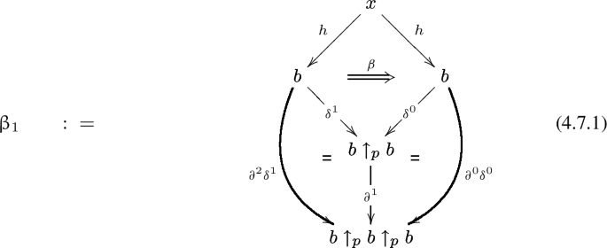
In order to prove Theorem 4.7, we consider the 2-cells defined in Lemma 4.6. Before defining them, it should be noted that:

Lemma 4.5

(${\ell _ *}\cdot \partial ^1$) Assume that p satisfies the condition of Proposition 4.2. The morphism ${\ell _ *}\cdot \partial ^1$ is the unique morphism such that the equations

$$\begin{aligned} \left( {\ell _ *}\partial ^1\right) \cdot \delta ^1 = t^2, \quad \left( {\ell _ *}\partial ^1\right) \cdot \delta ^0 = \textrm{id}_ b\quad \text{ and }\quad \textrm{id}_ {{\ell _ *}\partial ^1} *\upalpha = \left( \textrm{id}_ {t} *\gamma \right) \cdot \gamma \end{aligned}$$

hold.

Proof

In fact, by the definitions of $\ell$ (see Proposition 4.1) and ${\ell _ *}$ (see Proposition 4.4), the equations

hold. Therefore, by the definition of $\partial ^1$ (see 2.8 and, more particularly, (2.8.3) and (2.8.4)), we get the results. $\square$

Lemma 4.6

($\uptheta$ and $\uplambda$) Assume that $p: e\rightarrow b$ satisfies the condition of Proposition 4.2. There are 2-cells

$$\begin{aligned} \uptheta : {\mathfrak {s}}^0 \Rightarrow \ell \,: b\uparrow _ p b\rightarrow b, \qquad \uplambda : {\ell _ *}\cdot \partial ^1\Rightarrow \ell \,: b\uparrow _ p b\rightarrow b \end{aligned}$$

such that the equations

$$\begin{aligned} \uptheta *\textrm{id}_ {\delta ^1} = \eta , \quad \uptheta *\textrm{id}_ {\delta ^0} = \textrm{id}_ {\textrm{id}_ b}, \quad \uplambda *\textrm{id}_ {\delta ^1} = m, \quad \uplambda *\textrm{id}_ {\delta ^0} = \textrm{id}_ {\textrm{id}_ b} \end{aligned}$$

are satisfied.

Proof

In fact, by the universal property of the opcomma object $b\uparrow _p b$ of p along itself:

• there is a unique 2-cell $\uptheta : {\mathfrak {s}}^0 \Rightarrow \ell$ such that $\uptheta *\textrm{id}_ {\delta ^1} = \eta$ and $\uptheta *\textrm{id}_ {\delta ^0} = \textrm{id}_ {\textrm{id}_ b}$, since

  $$\begin{aligned} \left( \textrm{id}_ \ell *\upalpha \right) \cdot \left( \eta *\textrm{id}_ p \right) = \gamma \cdot \left( \eta *\textrm{id}_ p \right) = \textrm{id}_ p = \textrm{id}_ {{\mathfrak {s}}^0 }*\upalpha \end{aligned}$$

  by the definitions of $\ell$, $\eta$ and ${\mathfrak {s}}^0$;

• there is a unique 2-cell $\uplambda : {\ell _ *}\cdot \partial ^1\Rightarrow \ell$ such that $\uplambda *\textrm{id}_ {\delta ^1} = m$ and $\uplambda *\textrm{id}_ {\delta ^0} = \textrm{id}_ {\textrm{id}_ b}$, since it follows from the definitions of $\ell$ and $m: t ^2\Rightarrow t$ that

  $$\begin{aligned} \left( \textrm{id}_ \ell *\upalpha \right) \cdot (m*\textrm{id}_ p ) = \gamma \cdot (m*\textrm{id}_ p ) = \gamma \cdot (\textrm{id}_ t *\gamma ) = \textrm{id}_ {{\ell _ *}\cdot \partial ^1}*\upalpha \end{aligned}$$

  by Lemma 4.5.

$\square$

Theorem 4.7

Assume that p satisfies the condition of Proposition 4.2. We get that the factorization defined in (2.13.2) is 2-naturally (in x) isomorphic to the factorization defined in (3.7.2).

Proof

Recall that (2.13.2) is the factorization of ${\mathbb {A}}(x, p )$ induced by the pair

$$\begin{aligned} \left( {\mathbb {A}}(x, p), {\mathbb {A}}(x, \upalpha ) \right) \end{aligned}$$

and the universal property of the lax descent category of ${\mathbb {A}}(x,\mathcal {H}_p -): \Delta _ \text {Str}\rightarrow {\textsf {Cat}}$; and (3.7.2) is the factorization of ${\mathbb {A}}(x, p )$ induced by the pair $({\mathbb {A}}(x, p ), {\mathbb {A}}(x, \gamma ))$ and the universal property of the Eilenberg–Moore category ${\mathbb {A}}(x, b) ^{{\mathbb {A}}(x, \texttt {t} ) }$ of the monad ${\mathbb {A}}(x, \texttt {t} )$.

Observe that, since $(\ell \dashv \delta ^0, \textrm{id}_ {\textrm{id}_ b}, {\overline{\upeta }} ): b\uparrow _ p b\rightarrow b$ is an adjunction by Proposition 4.2, for each morphism $h: x\rightarrow b$ of ${\mathbb {A}}$ (i.e. for each object of ${\mathbb {A}}(x, b )$), there is a bijection

$$\begin{aligned} {\mathbb {A}}(x, b\uparrow _ p b )(\delta ^1\cdot h, \delta ^0\cdot h )\cong {\mathbb {A}}(x, b)(\ell \cdot \delta ^1\cdot h, \ell \cdot \delta ^0\cdot h ) = {\mathbb {A}}(x, b)(t\cdot h, h ) \end{aligned}$$

defined by $\beta \mapsto \textrm{id}_ {\ell }*\beta$, that is to say, the mate correspondence under the identity adjunction $\textrm{id}_ x\dashv \textrm{id}_ x$ and the adjunction $(\ell \dashv \delta ^0, \textrm{id}_ {\textrm{id}_ b}, {\overline{\upeta }} )$, see Remark 3.15.

Given an object h of ${\mathbb {A}}(x, b)$, we prove below that a 2-cell $\beta : \delta ^1\cdot h\Rightarrow \delta ^0\cdot h$ satisfies the descent associativity and identity ((2.7.2) and (2.7.3)) w.r.t. $\mathcal {H}_p$ if and only if its corresponding 2-cell $\textrm{id}_ {\ell }*\beta$ satisfies the algebra associativity and identity equations w.r.t. $\texttt {t}$ ((3.1.4) and (3.1.5)).

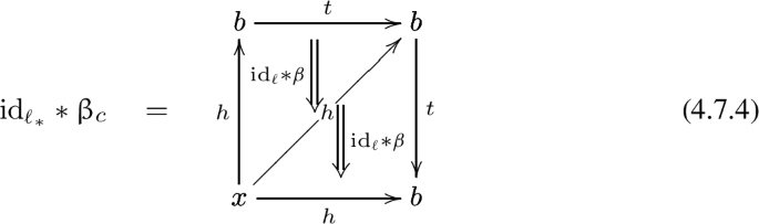
• 1. Observe that, given a 2-cell $\beta : \delta ^1\cdot h\Rightarrow \delta ^0\cdot h$, by the definition of $\uptheta$ in Lemma 4.6, we get that

  $$\begin{aligned} \textrm{id}_ {{\mathfrak {s}}^0}*\beta= & {} \textrm{id}_ {{\mathfrak {s}}^0\cdot \delta ^0 \cdot h}\cdot \left( \textrm{id}_ {{\mathfrak {s}}^0}*\beta \right) \\= & {} \left( \textrm{id}_ { \textrm{id}_ b }*\textrm{id}_ h \right) \cdot \left( \textrm{id}_ {{\mathfrak {s}}^0}*\beta \right) \\= & {} \left( \left( \uptheta *\textrm{id}_ {\delta ^0} \right) *\textrm{id}_ h \right) \cdot \left( \textrm{id}_ {{\mathfrak {s}}^0}*\beta \right) \\= & {} \left( \uptheta *\textrm{id}_ {\delta ^0 \cdot h}\right) \cdot \left( \textrm{id}_ {{\mathfrak {s}}^0}*\beta \right) \\= & {} \uptheta *\beta \end{aligned}$$

  which, by the interchange law, is equal to the left side of the equation

  $$\begin{aligned} \left( \textrm{id}_ \ell *\beta \right) \cdot \left( \uptheta *\textrm{id}_ {\delta ^1}*\textrm{id}_ h \right) = \left( \textrm{id}_ \ell *\beta \right) \cdot \left( \eta *\textrm{id}_ h \right) \end{aligned}$$

  which holds by Lemma 4.6. Thus, of course, $\left( \textrm{id}_ \ell *\beta \right) \cdot \left( \eta *\textrm{id}_ h \right)$ is the identity on h if and only if $\textrm{id}_ {{\mathfrak {s}}^0}*\beta = \left( \textrm{id}_ \ell *\beta \right) \cdot \left( \eta *\textrm{id}_ h \right)$ is the identity on h as well. This proves that $\left( h, \beta \right)$ satisfies the descent identity (2.7.3) w.r.t. $\mathcal {H}_p$ if and only if $\left( h, \textrm{id}_ \ell *\beta \right)$ satisfies the algebra identity equation w.r.t. $\texttt {t}$ (3.1.5).

• 2. Recall the adjunction $\left( {\ell _ *}\dashv \partial ^0 \delta ^0,\, \textrm{id}_{\textrm{id}_b},\, \uprho \right)$ of Proposition 4.4. Given a 2-cell $\beta : \delta ^1\cdot h\Rightarrow \delta ^0\cdot h$, consider the 2-cells defined by the pastings below.

  

  

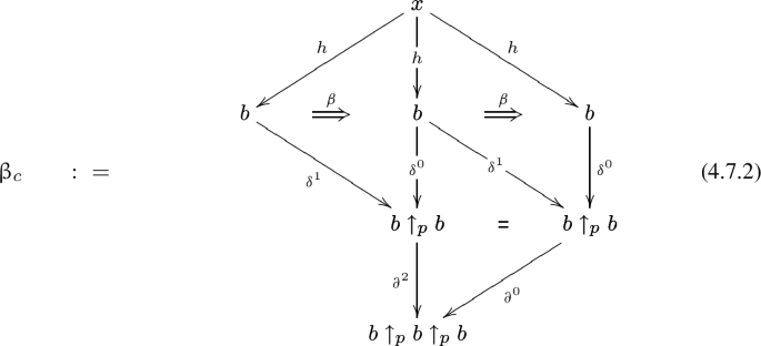
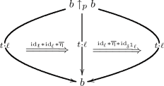
  We have that $\upbeta _c = \upbeta _ 1$ if, and only if, $\left( h, \beta \right)$ satisfies the descent associativity (2.7.2) w.r.t. $\mathcal {H}_p$. Therefore, by the mate correspondence under the identity adjunction $\textrm{id}_ x \dashv \textrm{id}_ x$ and the adjunction $({\ell _ *}\dashv \partial ^0 \delta ^0, \textrm{id}_{\textrm{id}_b}, \uprho )$, we conclude that $\left( h, \beta \right)$ satisfies the descent associativity (2.7.2) w.r.t. $\mathcal {H}_p$ if, and only if,

  $$\begin{aligned} \textrm{id}_ {{\ell _ *}}*\upbeta _ c = \textrm{id}_ {{\ell _ *}}*\upbeta _ 1. \end{aligned}$$

  (4.7.3)

  Now, we observe that:

  • (a) Since ${\ell _ *}\cdot \partial ^2 = t\cdot \ell$ and ${\ell _ *}\cdot \partial ^0 = \ell$, we have that

    

  • (b) By Lemma 4.6,

    $$\begin{aligned} \textrm{id}_{{\ell _ *}}*\upbeta _ 1= & {} \left( \textrm{id}_ {{\ell _ *}\partial ^1}*\beta \right) \\= & {} \left( \textrm{id}_ {\textrm{id}_ b}*\textrm{id}_ h \right) \cdot \left( \textrm{id}_ {{\ell _ *}\partial ^1}*\beta \right) \\= & {} \left( \uplambda *\textrm{id}_ {\delta ^0 }*\textrm{id}_ h \right) \cdot \left( \textrm{id}_ {{\ell _ *}\partial ^1}*\beta \right) \end{aligned}$$

    which, by the interchange law and Lemma 4.6, is equal to

    

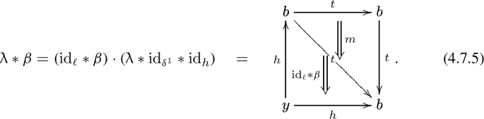
  Therefore (4.7.3) holds if, and only if, the pasting (4.7.4) is equal to (4.7.5).

  This completes the proof that $\left( h, \beta \right)$ satisfies descent associativity w.r.t. $\mathcal {H}_p$ if, and only if, $\textrm{id}_ \ell *\beta$ satisfies the algebra associativity (3.1.4) w.r.t. $\texttt {t}$.

The above implies that the association $(h, \beta )\mapsto (h, \textrm{id}_ \ell *\beta )$ gives a bijection between the objects of $\mathrm{\mathsf lim}\left( \mathfrak {D}, {\mathbb {A}}(x, \mathcal {H}_ p - )\right)$ and ${\mathbb {A}}(x, b)^{{\mathbb {A}}(x, \texttt {t} )}$.

Given objects $(h _ 1, \beta _1 )$ and $(h_0, \beta _ 0 )$ of $\mathrm{\mathsf lim}\left( \mathfrak {D}, {\mathbb {A}}(x, \mathcal {H}_ p - )\right)$, by the mate correspondence under the identity adjunction and $\ell \dashv \delta ^0$, a 2-cell

$$\begin{aligned} \xi : h_1\Rightarrow h_0: x\rightarrow b \end{aligned}$$

satisfies the equation

if and only if the mate of the left side is equal to the mate of the right side, which means

which is precisely the condition of being a morphism of algebras in ${\mathbb {A}}(x, b)^{{\mathbb {A}}(x, \texttt {t} )}$. In other words, this proves that $\xi$ gives a morphism between $(h _ 1, \beta _1 )$ and $(h_0, \beta _ 0 )$ in $\mathrm{\mathsf lim}\left( \mathfrak {D}, {\mathbb {A}}(x, \mathcal {H}_ p - )\right)$ if and only if it gives a morphism between $(h _ 1, \textrm{id}_ \ell *\beta _1 )$ and $(h_0, \textrm{id}_ \ell *\beta _0 )$ in ${\mathbb {A}}(x, b)^{{\mathbb {A}}(x, \texttt {t} )}$.

Finally, given the facts above, we can conclude that we actually can define

$$\begin{aligned} \mathrm{\mathsf lim}\left( \mathfrak {D}, {\mathbb {A}}(x, \mathcal {H}_ p - )\right)\rightarrow & {} {\mathbb {A}}(x, b)^{{\mathbb {A}}(x, \texttt {t} )}\\ (h, \beta )\mapsto & {} (h, \textrm{id}_\ell *\beta ) \\ \xi\mapsto & {} \xi \end{aligned}$$

which is clearly functorial and, hence, it defines an invertible functor (since it is bijective on objects and fully faithful as proved above).

This invertible functor is 2-natural in x, giving a 2-natural isomorphism between (2.13.2) and (3.7.2). $\square$

Theorem 4.8

(Main Theorem) Assume that $\textrm{ran}_p p$ exists and is preserved by the morphism $\delta ^0: b\rightarrow b\uparrow _p b$. We have that the semantic factorization (3.6.3) of p is isomorphic to the semantic lax descent factorization (2.11.1) of p, either one existing if the other does.

Proof

It is clearly a direct consequence of Theorem 4.7. $\square$

Recall that, since the result above works for any 2-category, we have the dual results. For instance, we have Theorems 4.9 and 4.10.

Theorem 4.9

(Codual) Let $l: b\rightarrow e$ be a morphism of ${\mathbb {A}}$ satisfying the following conditions:

• 1. ${\mathbb {A}}$ has the two-dimensional cokernel diagram of l;

• 2. the left Kan extension $\textrm{lan}_ l l$ of l along itself exists (that is to say, l has the density comonad);

• 3. the left Kan extension $\textrm{lan}_ l l$ is preserved by $\delta _ {l\uparrow l} ^1: e\rightarrow l\uparrow l$.

The diagram of the co-semantic factorization of l is isomorphic to the semantic lax descent factorization of l either one existing if the other does.

Proof

By the observations on the self-coduality of the factorization in Remark 2.15, we get the result from Theorem 4.8. $\square$

Theorem 4.10

(Dual) Let $l: b\rightarrow e$ be a morphism of ${\mathbb {A}}$ satisfying the following conditions:

• 1. ${\mathbb {A}}$ has the higher kernel of l;

• 2. the right lifting of l through itself exists (that is to say, l has the op-codensity monad);

• 3. the right lifting of l through itself is respected by the arrow $\delta ^ {l\downarrow l} _0: l\downarrow l\rightarrow b$.

The diagram of the op-semantic factorization of l is 2-naturally isomorphic to the semantic lax codescent factorization of l (see Remark 2.15 and (2.15.1)).

As a consequence of Theorem 4.8 and its duals, by Proposition 4.3, we get:

Theorem 4.11

(Adjunction) Let $(\mathfrak {l} \dashv \mathfrak {p}, \varepsilon , \eta ): \mathfrak {b}\rightarrow \mathfrak {e}$ be an adjunction in ${\mathbb {A}}$. We have the following:

• 1. if ${\mathbb {A}}$ has the two-dimensional cokernel diagram of $\mathfrak {p}$, then the semantic lax descent factorization (2.11.1) of $\mathfrak {p}$ coincides up to isomorphism with the usual factorization of $\mathfrak {p}$ through the Eilenberg–Moore object, either one existing if the other does;

• 2. if ${\mathbb {A}}$ has the two-dimensional kernel diagram of $\mathfrak {l}$, then the semantic lax codescent factorization of $\mathfrak {l}$ coincides up to isomorphism with the usual factorization of $\mathfrak {l}$ through the Kleisli object, either one existing if the other does;

• 3. if ${\mathbb {A}}$ has the two-dimensional cokernel diagram of $\mathfrak {l}$, then the semantic lax descent factorization of $\mathfrak {l}$ coincides up to isomorphism with the usual factorization of $\mathfrak {l}$ through the co-Eilenberg–Moore object, either one existing if the other does;

• 4. if ${\mathbb {A}}$ has the two-dimensional kernel diagram of $\mathfrak {p}$, then the semantic lax codescent factorization of $\mathfrak {p}$ coincides up to isomorphism with the usual factorization of $\mathfrak {p}$ through the co-Kleisli object, either one existing if the other does.

5.1 (Counter)Examples of Morphisms Satisfying Proposition 4.2

Even ${\textsf {Cat}}$ has morphisms that do not satisfy the condition of Proposition 4.2.

For instance, the inclusion of the domain $d^1: \textsf {1}\rightarrow \textsf {2}$ has the codensity monad. More precisely $\textrm{ran}_{d^1} d^1$ is given by $\textrm{id}_ {\textsf {2}}: \textsf {2}\rightarrow \textsf {2}$ with the unique 2-cell (natural transformation) $d^1\Rightarrow d^1$. However, in this case, $\delta _ {d^1\uparrow d^1} ^0$ is the inclusion

which does not preserve the terminal object, since $\textsf {2}$ has terminal object and $d^1\uparrow d^1$ does not. Hence $\delta _ {d^1\uparrow d^1} ^0$ does not have a left adjoint. Actually, it even does not have a codensity monad. Therefore the condition of Proposition 4.2 does not hold for $d^1: \textsf {1}\rightarrow \textsf {2}$.

It should be noted that $d ^1$ is left adjoint to $s ^0$ and, hence, it does satisfy the codual of the condition of Proposition 4.2. More precisely, since $d ^1: \textsf {1}\rightarrow \textsf {2}$ is a left adjoint functor, it satisfies the hypothesis of 3 of Theorem 4.11. Hence the co-semantic factorization (usual factorization through the category of coalgebras) coincides with the semantic lax descent factorization of $d ^1$. These factorizations are given by

$$\begin{aligned} d ^1 = d^1 \circ \textrm{id}_ {\textsf {1} }. \end{aligned}$$

By Proposition 4.3, any right adjoint morphism satisfies Proposition 4.2. The converse is false, that is to say, the condition of Proposition 4.2 does not imply the existence of a left adjoint. There are simple counterexamples in ${\textsf {Cat}}$. In order to construct such an example, we observe that:

Lemma 4.13

Let $\iota _ e: e\rightarrow \textsf {1}$ be a functor between a small category e and the terminal category. We have that $\textrm{ran}_ {\iota _ e}\iota _ e$ and $\textrm{lan}_ {\iota _ e}\iota _ e$ are given by the identity on $\textsf {1}$. Therefore the semantic factorization and the co-semantic factorization are both given by

$$\begin{aligned} \iota _ e = \textrm{id}_ {\textsf {1} }\circ \iota _ e. \end{aligned}$$

Moreover, $\iota _ e$ has a left adjoint (right adjoint) if and only if e has initial object (terminal object).

Since the thin category ${\mathbb {R}}$ corresponding to the usual preordered set of real numbers does not have initial or terminal objects, the only functor $\iota _ {\mathbb {R}}: {\mathbb {R}}\rightarrow \textsf {1}$ does not have any adjoint. However, it is clear that every functor $\textsf {1}\rightarrow b$ preserves the (conical) limit of ${\mathbb {R}}\rightarrow \textsf {1}$ and, hence, any such functor does preserve $\textrm{ran}_ {\iota _ {\mathbb {R}}} \iota _ {\mathbb {R}}$. In particular, $\iota _ {\mathbb {R}}$ does satisfy Proposition 4.2.

This proves that, although the morphism $\iota _ {\mathbb {R}}: {\mathbb {R}}\rightarrow \textsf {1}$ does not satisfy any of the versions of Theorem 4.11, it does satisfy the conditions of Theorem 4.8. Hence the semantic lax descent factorization of $\iota _ {\mathbb {R}}$ (Eq. 2.11.1) coincides with the semantic factorization of $\iota _ {\mathbb {R}}$. In this case, by Lemma 4.13, both factorizations are given by

$$\begin{aligned} \iota _ {\mathbb {R}} = \textrm{id}_ {\textsf {1} }\circ \iota _ {\mathbb {R}}. \end{aligned}$$

Remark 4.14

Although (by Lemma 4.13) the codensity monad and the density comonad of $\iota _{\textsf {1}\sqcup \textsf {1}}$ are the identity on $\textsf {1}$, the functor $\iota _{\textsf {1}\sqcup \textsf {1}}$ does not satisfy the condition of Proposition 4.2 nor the codual.

In fact, a functor $\textsf {1} \rightarrow b$ preserves $\textrm{ran}_ {\iota _{\textsf {1}\sqcup \textsf {1}} } \iota _{\textsf {1}\sqcup \textsf {1}}$ ($\textrm{lan}_{\iota _{\textsf {1}\sqcup \textsf {1}} } \iota _{\textsf {1}\sqcup \textsf {1}}$) if and only if $\textsf {1} \rightarrow b$ preserves binary products (binary coproducts) which does happen if and only if the image of $\textsf {1}\rightarrow b$ is a preterminal (preinitial) object (see [20, Remark 4.5] for instance).

The opcomma category of $\iota _{\textsf {1}\sqcup \textsf {1}}$ along itself is the category with two distinct objects and two parallel arrows between them: hence it does not have any preterminal or preinitial objects. This shows that neither $\textrm{ran}_ {\iota _{\textsf {1}\sqcup \textsf {1}}} \iota _{\textsf {1}\sqcup \textsf {1}}$ nor $\textrm{lan}_{\iota _{\textsf {1}\sqcup \textsf {1}}} \iota _{\textsf {1}\sqcup \textsf {1}}$ is preserved by any functor $\textsf {1}\rightarrow \iota _{\textsf {1}\sqcup \textsf {1}} \uparrow \iota _{\textsf {1}\sqcup \textsf {1}}$.

This proves that the functor $\iota _{\textsf {1}\sqcup \textsf {1}}: \textsf {1}\sqcup \textsf {1}\rightarrow \textsf {1}$ does not satisfy the hypotheses of Theorem 4.8. Since ${\textsf {Cat}}$ has Eilenberg–Moore objects, two-dimensional cokernel diagrams and lax descent objects, we have the semantic lax descent factorization of $\iota _{\textsf {1}\sqcup \textsf {1}}$ and the semantic factorization. However, in this case, they do not coincide. More precisely, they are respectively given by the commutative triangles below.

6 Monadicity and Effective Faithful Morphisms

In this section, we show direct consequences of Theorem 4.8 on monadicity. Henceforth, whenever a 2-category ${\mathbb {A}}$ has the two-dimensional cokernel diagram $\mathcal {H}_ p$ of a morphism $p: e\rightarrow b$, we use the notation of 2.8 and 2.9. If ${\mathbb {A}}$ has the two-dimensional kernel diagram of a morphism $l: e\rightarrow b$, we use the notation of Remark 2.15.

Recall that a morphism $\mathfrak {p}: \mathfrak {e}\rightarrow \mathfrak {b}$ of a 2-category ${\mathbb {A}}$ is an equivalence if there is are a morphism $\mathfrak {l}: \mathfrak {b}\rightarrow \mathfrak {e}$ and invertible 2-cells $\mathfrak {l}\mathfrak {p}\Rightarrow \textrm{id}_ \mathfrak {e}$, $\textrm{id}_ \mathfrak {b} \Rightarrow \mathfrak {p}\mathfrak {l}$. It is a basic coherence result the fact that, whenever we have such a data, we can actually get an adjunction $\mathfrak {l} \dashv \mathfrak {p}$ and an adjunction $\mathfrak {p}\dashv \mathfrak {l}$ with invertible units and invertible counits. These adjunctions are called adjoint equivalences.

Definition 5.1

Let $\mathcal {A}: \Delta _ \text {Str}\rightarrow {\mathbb {A}}$ be a 2-functor. We say that the pair

(5.1.1)

in which p is a morphism and $\uppsi$ is a 2-cell, is effective w.r.t. $\mathrm{\mathsf lim}( \mathfrak {D}, \mathcal {A})$ if the following statements hold:

• ${\mathbb {A}}$ has the lax descent object $\mathrm{\mathsf lim}( \mathfrak {D}, \mathcal {A})$;

• the pair $(p, \uppsi )$ satisfies the descent associativity (2.7.2) and identity (2.7.3) w.r.t. $\mathcal {A}$;

• the induced factorization is such that $p^{( \mathcal {A}, \uppsi ) }$ is an equivalence.

Definition 5.2

(effective faithful morphism) Let $p:e\rightarrow b$ be a morphism of a 2-category ${\mathbb {A}}$. The morphism p is an effective faithful morphism of ${\mathbb {A}}$ if the following statements hold:

• ${\mathbb {A}}$ has the two-dimensional cokernel diagram of p;

• ${\mathbb {A}}$ has the lax descent object of the two-dimensional cokernel diagram $\mathcal {H}_ p$;

• the semantic lax descent factorization (2.11.1) of p, , is such that $p ^\mathcal {H}$ is an equivalence, that is to say, $(p, \upalpha )$ is effective w.r.t. $\mathcal {H}_p$.

Remark 5.3

The terminology of Definition 5.2 is motivated by the 1-dimensional case. In a category with suitable pushouts and coequalizers, every morphism p has a factorization induced by the equalizer of the “cokernel pair”

of p. If the morphism p is itself the equalizer, p is said to be an effective monomorphism.

Remark 5.4

The concept of effective faithful morphism was already considered in [31, pag. 142] under the name effective descent morphism. The terminology of [31, pag. 142] does not agree with the usual terminology of Grothendieck descent theory within the context of [9, 19]. Since the present work is intended to be applied to the context of [19], we adopt the alternative terminology.

Remark 5.5

If a morphism $p: e\rightarrow b$ of a 2-category ${\mathbb {A}}$ is effective w.r.t. any 2-functor $\mathcal {A}: \Delta _ \text {Str}\rightarrow {\mathbb {A}}$, it is clear that p is faithful. More precisely, in this case, for any object x, ${\mathbb {A}}(x, p ): {\mathbb {A}}(x, e)\rightarrow {\mathbb {A}}(x,b)$ is faithful. In particular, if p is an effective faithful morphism, then p is faithful.

By Remark 2.15, the codual of (2.11.1) of a morphism p gives the same factorization, provided that it exists. Hence, we have:

Lemma 5.6

(Self-coduality) Let p be a morphism of a 2-category ${\mathbb {A}}$. The morphism p is an effective faithful morphism in ${\mathbb {A}}$ if and only if the morphism corresponding to p is an effective faithful morphism in ${\mathbb {A}}^\textrm{co}$.

Definition 5.7

(Duality: effective op-faithful morphism) Let $p: e\rightarrow b$ be a morphism of a 2-category ${\mathbb {A}}$. The morphism p is an effective op-faithful morphism of ${\mathbb {A}}$ if the morphism corresponding to p is an effective faithful morphism in ${\mathbb {A}}^\textrm{op}$.

Definition 5.8

(Monadicity, comonadicity, Kleisli morphism) Let $p: e\rightarrow b$ be a morphism of a 2-category ${\mathbb {A}}$. We say that p is monadic if the following statements hold:

• p has a codensity monad $\texttt {t} = (t, m, \eta )$;

• ${\mathbb {A}}$ has the Eilenberg–Moore object of $\texttt {t}$;

• the semantic factorization of is such that $p^\texttt {t}$ is an equivalence.

Dually, $l: b\rightarrow e$ is a Kleisli morphism if the corresponding morphism in ${\mathbb {A}}^\textrm{op}$ is monadic, while l is comonadic if its corresponding morphism in ${\mathbb {A}}^\textrm{co}$ is monadic.

By Theorem 4.8 and its dual versions, we get the following characterizations of monadicity, comonadicity and Kleisli morphisms:

Corollary 5.9

(Monadicity theorem) Assume that ${\mathbb {A}}$ has the two-dimensional cokernel diagram of a morphism $p: e\rightarrow b$.

• 1. provided that $\textrm{ran}_p p$ exists and is preserved by $\delta ^0$, p is monadic if and only if p is an effective faithful morphism;

• 2. provided that $\textrm{lan}_p p$ exists and is preserved by $\delta ^1$, p is comonadic if and only if p is an effective faithful morphism.

Proof

The first result follows immediately from the definitions and from Theorem 4.8. The second one is just its codualization (see Lemma 5.6, Theorem 4.9 and Remark 2.15). $\square$

Corollary 5.10

(Characterization of Kleisli morphisms) Assume that ${\mathbb {A}}$ has the higher kernel of a morphism $l: b\rightarrow e$.

• 1. assuming that $\textrm{rlift}_l l$ exists and is respected by $\delta _0^{l\downarrow l}$, l is a Kleisli morphism if and only if l is an effective op-faithful morphism;

• 2. assuming that $\textrm{llift}_p p$ exists and is respected by $\delta _1^{l\downarrow l}$, l is comonadic if and only if l is an effective op-faithful morphism.

It is a well known fact that, whenever a morphism is monadic in a 2-category ${\mathbb {A}}$, it has a left adjoint. In our setting, if p is monadic as in Definition 5.8, the existence of a left adjoint follows from: (1) since $p^\texttt {t}$ is an equivalence, it has a left adjoint; (2) has always a left adjoint induced by the underlying morphism of the monad $t: b\rightarrow b$, the multiplication $m: t^2\Rightarrow t$ and the universal property of $b ^\texttt {t}$; and (3) composition of right adjoint morphisms is right adjoint. From this fact and Theorem 4.11, we get cleaner versions of our monadicity results:

Corollary 5.11

(Monadicity theorem) Assume that the 2-category ${\mathbb {A}}$ has the two-dimensional cokernel diagram of a morphism p.

• 1. The morphism p is monadic if and only if p has a left adjoint and p is an effective faithful morphism.

• 2. The morphism p is comonadic if and only if p has a right adjoint and p is an effective faithful morphism.

Corollary 5.12

(Characterization of Kleisli morphisms) Assume that the 2-category ${\mathbb {A}}$ has the two-dimensional kernel diagram of a morphism l.

• 1. The morphism l is a co-Kleisli morphism if and only if l has a left adjoint and l is an effective op-faithful morphism.

• 2. The morphism l is Kleisli morphism if and only if l has a right adjoint and l is an effective op-faithful morphism.

Remark 5.13

(Monadicity vs comonadicity) It should be noted that, unlike Beck’s monadicity theorem in ${\textsf {Cat}}$, the condition to get monadicity from a right adjoint morphism coincides with the condition to get comonadicity from a left adjoint morphism; namely, to be an effective faithful morphism. Of course, as a consequence, we get that, under the conditions of Corollary 5.11, if the morphism p has a left and a right adjoint morphism, the following statements are equivalent:

• (i) p is an effective faithful morphism;

• (ii) p is monadic;

• (iii) p is comonadic.

Remark 5.14

(Beck’s monadicity theorem vs formal monadicity theorem) Beck’s monadicity theorem states that, in ${\textsf {Cat}}$, a functor p is monadic if and only if p has a left adjoint and p creates absolute coequalizers. By our monadicity theorem, we can conclude that, provided that a functor $p:e\rightarrow b$ has a left adjoint, p creates absolute coequalizers if and only if p is an effective faithful morphism in ${\textsf {Cat}}$.

However, the effective faithful morphisms in ${\textsf {Cat}}$ are not characterized by the property of creation of absolute coequalizers. For instance, this follows from the fact that, by Lemma 5.6, the concept of effective faithful morphism is self codual, while the property of creation of absolute coequalizers is not self dual.

More precisely, one of the key aspects of duality in 1-dimensional category theory is that the usual 2-functor $\textrm{op}$ given by

is invertible. Therefore a functor $p ^\textrm{op}: e ^\textrm{op}\rightarrow b ^\textrm{op}$ is an effective faithful morphism in ${\textsf {Cat}}$ if and only if the morphism $p: e\rightarrow b$ is an effective faithful morphism in ${\textsf {Cat}}^\textrm{co}$. Moreover, by Lemma 5.6, the morphism p is an effective faithful morphism in ${\textsf {Cat}}^\textrm{co}$ if and only if the corresponding morphism (functor) p is an effective faithful morphism in ${\textsf {Cat}}$. Hence, by abuse of notation, p is an effective faithful morphism in ${\textsf {Cat}}$ if and only if $p ^\textrm{op}$ is an effective faithful morphism in ${\textsf {Cat}}$.

It is clear that a functor $p: e\rightarrow b$ creates absolute coequalizers if and only if the functor corresponding to $p^\textrm{op}: e^\textrm{op}\rightarrow b ^\textrm{op}$ creates absolute equalizers. Since there are functors that create absolute coequalizers but do not create absolute equalizers, the property of creation of absolute equalizers is not self dual. It follows, then, that there are functors that do create absolute coequalizers but are not effective faithful morphisms.

For instance, consider the usual forgetful functor between the category of free groups and the category of sets. This functor reflects isomorphisms and preserves equalizers: hence, since the category of free groups has equalizers, this forgetful functor creates all equalizers. However, since it has a left adjoint, it does not create absolute coequalizers and it is not an effective faithful morphism in ${\textsf {Cat}}$ (otherwise, it would be monadic). Therefore the image of the morphism corresponding to this functor in ${\textsf {Cat}}^\textrm{co}$ by $\textrm{op}$ is a functor that creates absolute coequalizers but it is not an effective faithful morphism in ${\textsf {Cat}}$.

Remark 5.15

(Characterization of effective faithful morphisms) In [31], Zawadowski gave the characterizations of effective faithful morphisms in some special 2-categories. Moreover, as a consequence of proof of [29, Proposition 3.1], the effective op-faithful morphisms in ${\textsf {Cat}}$ are precisely the functors that are essentially surjective on objects.

References

Adámek, J., Sousa, L.: A formula for codensity monads and density comonads. Appl. Categ. Struct. 26(5), 855–872 (2018)
Barr, M., Wells, C.: Toposes, triples and theories. Repr. Theory Appl. Categ. TAC(12), x+288 (2005). (Corrected reprint of the 1985 original)
Bénabou, J.: Introduction to bicategories. In: Reports of the Midwest Category Seminar, pp. 1–77. Springer, Berlin (1967)
Bénabou, J., Roubaud, J.: Monades et descente. C. R. Acad. Sci. Paris Sér. A-B 270, A96–A98 (1970)
Dubuc, E.: Kan Extensions in Enriched Category Theory. Lecture Notes in Mathematics, vol. 145. Springer, Berlin (1970)
Eilenberg, S., Moore, J.C.: Adjoint functors and triples. Ill. J. Math. 9, 381–398 (1965)
Grothendieck, A.: Technique de descente et théorèmes d’existence en géometrie algébrique. I. Généralités. Descente par morphismes fidèlement plats. In: Séminaire Bourbaki, vol. 5, pp. 190, 299–327. French Mathematical Society, Paris (1995)
Janelidze, G., Tholen, W.: Facets of descent. I. Appl. Categ. Struct. 2(3), 245–281 (1994)
Janelidze, G., Tholen, W.: Facets of descent. II. Appl. Categ. Struct. 5(3), 229–248 (1997)
Janelidze, G., Tholen, W.: Facets of descent. III. Monadic descent for rings and algebras. Appl. Categ. Struct. 12(5–6), 461–477 (2004)
Kelly, G.M.: Elementary observations on \(2\)-categorical limits. Bull. Austral. Math. Soc. 39(2), 301–317 (1989)
Kelly, G.M., Street, R.: Review of the elements of \(2\)-categories. Category Seminar (Proc. Sem., Sydney, 1972/1973). Lecture Notes in Mathematics, vol. 420, pp. 75–103 (1974)
Kleisli, H.: Every standard construction is induced by a pair of adjoint functors. Proc. Am. Math. Soc. 16, 544–546 (1965)
Lack, S.: Codescent objects and coherence. J. Pure Appl. Algebra 175(1–3), 223–241 (2002). (Special volume celebrating the 70th birthday of Professor Max Kelly)
Lawvere, F.W.: Functorial semantics of algebraic theories and some algebraic problems in the context of functorial semantics of algebraic theories. Repr. Theory Appl. Categ. TAC(5), 1–121 (2004). (Reprint of the Ph.D. thesis, Columbia University, 1963 and in Reports of the Midwest Category Seminar II, 1968, 41–61, Springer-Verlag, with author’s comments (2004))
Leinster, T.: Codensity and the ultrafilter monad. Theory Appl. Categ. 28(13), 332–370 (2013)
Lucatelli Nunes, F.: On biadjoint triangles. Theory Appl. Categ. 31(9), 217–256 (2016)
Lucatelli Nunes, F.: On lifting of biadjoints and lax algebras. Categ. Gen. Algebraic Struct. Appl. 9(1), 29–58 (2018)
Lucatelli Nunes, F.: Pseudo-Kan extensions and descent theory. Theory Appl. Categ. 33(15), 390–444 (2018)
Lucatelli Nunes, F.: Pseudoalgebras and non-canonical isomorphisms. Appl. Categ. Struct. 27(1), 55–63 (2019)
Lucatelli Nunes, F.: Descent data and absolute Kan extensions. Theory Appl. Categ. 37(18), 530–561 (2021)
Mac Lane, S.: Categories for the Working Mathematician. Graduate Texts in Mathematics, vol. 5, 2nd edn. Springer, New York (1998)
Power, A.J.: A \(2\)-categorical pasting theorem. J. Algebra 129(2), 439–445 (1990)
Reiterman, J., Tholen, W.: Effective descent maps of topological spaces. Topol. Appl. 57(1), 53–69 (1994)
Street, R.: The formal theory of monads. J. Pure Appl. Algebra 2(2), 149–168 (1972)
Street, R.: Two constructions on lax functors. Cahiers Topologie Géom. Différentielle 13, 217–264 (1972)
Street, R.: Elementary cosmoi. I. In: Category Seminar (Proc. Sem., Sydney, 1972/1973). Lecture Notes in Mathematics, vol. 420, pp. 134–180. Springer, Berlin (1974)
Street, R.: Limits indexed by category-valued \(2\)-functors. J. Pure Appl. Algebra 8(2), 149–181 (1976)
Street, R.: Categorical and combinatorial aspects of descent theory. Appl. Categ. Struct. 12(5–6), 537–576 (2004)
Street, R., Walters, R.: Yoneda structures on 2-categories. J. Algebra 50(2), 350–379 (1978)
Zawadowski, M.W.: Descent and duality. Ann. Pure Appl. Logic 71(2), 131–188 (1995)
Acknowledgements
I am grateful to the Coimbra Category Theory Group for their unfailing support. I am also thankful to the Software Technology Group at Utrecht University for their welcoming and supportive environment. This work was realized during my postdoctoral fellowship at the Centre for Mathematics, University of Coimbra, in 2018. My ideas and results for this project were positively influenced by the peaceful and inspiring atmosphere I found there. I want to give special thanks to Marino Gran and Tim Van der Linden, who warmly hosted me at Université catholique de Louvain in May 2018, where my ideas and work for this project started. In my stay there, I found a very encouraging and productive environment. Maria Manuel Clementino made my stay at UCLouvain even more memorable, allowing me to work with her on exciting problems about Janelidze-Galois Theory. My discussions on examples of codensity monads with her and Eduardo Dubuc, whom I also wish to thank, were instrumental in coming up with counterexamples to some tempting but wrong strengthening of some of the present paper’s results. After publishing this work, I have received several questions and suggestions for future work, terminology and bibliography. In these directions, I am specially thankful to George Janelidze, Zurab Janelidze and Steve Lack. I want to thank Eduardo Ochs for taking his valuable time to teach me about his Dednat6 LaTeX package. During the revision of the present paper, Dednat6 proved very efficient to write and edit diagrams quickly.
Author information
Authors and Affiliations
Corresponding author
Additional information
Communicated by Maria Manuel Clementino.
Publisher's Note
Springer Nature remains neutral with regard to jurisdictional claims in published maps and institutional affiliations.
This research was partially supported by the Institut de Recherche en Mathématique et Physique (IRMP, UCLouvain, Belgium), and by the Centre for Mathematics of the University of Coimbra - UIDB/00324/2020, funded by the Portuguese Government through FCT/MCTES.
This work was also supported through the programme “Oberwolfach Leibniz Fellows” by the Mathematisches Forschungsinstitut Oberwolfach in 2022.
Rights and permissions
Open Access This article is licensed under a Creative Commons Attribution 4.0 International License, which permits use, sharing, adaptation, distribution and reproduction in any medium or format, as long as you give appropriate credit to the original author(s) and the source, provide a link to the Creative Commons licence, and indicate if changes were made. The images or other third party material in this article are included in the article’s Creative Commons licence, unless indicated otherwise in a credit line to the material. If material is not included in the article’s Creative Commons licence and your intended use is not permitted by statutory regulation or exceeds the permitted use, you will need to obtain permission directly from the copyright holder. To view a copy of this licence, visit http://creativecommons.org/licenses/by/4.0/.
About this article
Cite this article
Lucatelli Nunes, F. Semantic Factorization and Descent. Appl Categor Struct 30, 1393–1433 (2022). https://doi.org/10.1007/s10485-022-09694-w
Received:
Accepted:
Published:
Issue Date:
DOI: https://doi.org/10.1007/s10485-022-09694-w
Keywords
- Formal monadicity theorem
- Formal theory of monads
- Codensity monads
- Semantic lax descent factorization
- Descent data
- Two-dimensional cokernel diagram
- Opcomma object
- Effective faithful morphism
- Bénabou–Roubaud theorem
- Lax descent category
- Two-dimensional limits