Homogenization of fundamental solutions for parabolic operators involving non-self-similar scales

Abstract

We establish the asymptotic expansion of the fundamental solutions with precise error estimates for second-order parabolic operators

$$\begin{aligned} \partial _t -\text {div}(A(x/\varepsilon , t/\varepsilon ^\ell )\nabla ), \quad \, 0<\varepsilon<1,\, 0<\ell <\infty ,\end{aligned}$$

in the case $\ell \ne 2,$ where the spatial and temporal variables oscillate on non-self-similar scales and do not homogenize simultaneously. To achieve the goal, we explore the direct quantitative two-scale expansions for the aforementioned operators, which should be of some independent interests in quantitative homogenization of parabolic operators involving multiple scales. In the self-similar case $\ell =2$, similar results have been obtained in Geng and Shen (Anal PDE 13(1): 147–170, 2020).

1 Introduction

We consider the asymptotic behavior of fundamental solutions to a family of second-order parabolic operators

$$\begin{aligned} \partial _t +{\mathcal {L}}_\varepsilon =\partial _t -\text {div}(A(x/\varepsilon , t/\varepsilon ^\ell )\nabla ) \quad \quad \text { in } {\mathbb {R}}^{d+1} , \end{aligned}$$

(1.1)

where $0<\varepsilon<1,0<\ell <\infty$, the coefficient tensor $A=A (z,\tau )=(A^{\alpha \beta }_{ij}(z,\tau ) ), 1\le i, j\le d, 1\le \alpha ,\beta \le m,$ is real, bounded measurable and satisfy

• Ellipticity condition: there exists $\mu >0$ such that

  $$\begin{aligned} \mu |\xi |^2\le A_{ij}^{\alpha \beta }(z,\tau ) \xi _i^\alpha \xi _j^\beta \le \frac{1}{\mu } |\xi |^2 \end{aligned}$$

  (1.2)

  for any matrix $\xi =(\xi _i^\alpha )\in {\mathbb {R}}^{m\times d}$ and a.e. $(z,\tau )\in {\mathbb {R}}^{d+1}$.

• Periodicity condition: for any $(y,s) \in {\mathbb {Z}}^{d+1}$ and a.e. $(z,\tau )\in {\mathbb {R}}^{d+1}$,

  $$\begin{aligned} A(z+y, \tau +s)=A (z,\tau ) ~. \end{aligned}$$

  (1.3)

Under the conditions (1.2) and (1.3), it is well known that $\partial _t +{\mathcal {L}}_\varepsilon$ G-converges to $\partial _t +{\mathcal {L}}_0$, which has constant coefficients and depends on $\ell$ in three different cases: $0<\ell <2, \ell =2,$ and $2<\ell <\infty$. See [1] and also Section 2 for the details.

Quantitative homogenization of (1.1) has aroused great interests in recent years. In the case $\ell =2$, where the spatial and temporal variables oscillate on self-similar scales, the uniform Hölder and Lipschitz estimates in homogenization were derived by Geng and Shen in [7], while the two-scale expansions with precise error estimates for the operators were studied in different contexts in [8, 14, 17, 20, 21]. In particular, the asymptotic expansion of the fundamental solutions to (1.1) with sharp error estimates was established in [9].

In the case $\ell \ne 2$, the scales of the spatial and temporal variables do not coincide with the scales of the parabolic operators. As a result, the temporal and spatial variables do not homogenize simultaneously [1], and the quantitative homogenization theory for (1.1) is therefore much more intricate. Few results on the quantitative theory is known until very recently [10]. In [10], Geng and Shen developed an effective approach to study the quantitative homogenization theory of (1.1). One of the key ideas is to introduce a family of intermediate operators

$$\begin{aligned} \partial _t -\text {div}\big (A (x/\varepsilon , t /(\lambda \varepsilon ^2) )\nabla \big ), \quad \lambda >0, \end{aligned}$$

(1.4)

which converts the original operator to the one with self-similar scales (for each fixed $\lambda$). Then by the quantitative two-scale expansions for (1.4) and some intricate estimates on the corresponding ($\lambda$-dependent) correctors, they were able to establish the convergence rate and the large-scale estimates for the original operator (1.1).

In this paper, we shall explore the direct quantitative two-scale expansions of (1.1) in the non-self-similar case $\ell \ne 2$, and study the quantitative homogenization theory without introducing the intermediate operators (1.4). To fix the idea, we study the asymptotic expansion of the fundamental solution $\Gamma _{\varepsilon }$ of (1.1). Our results, combined with those in [9] for the case $\ell =2$, provide the whole view of asymptotic expansions of the fundamental solutions to (1.1).

Since the homogenized operator $\partial _t+{\mathcal {L}}_0$ has constant coefficients. It is well known that the matrix of fundamental solution $\Gamma _0(x,t;y,s)$ exists, and for any $x,y\in {\mathbb {R}}^{d}, -\infty<s<t<\infty$, and $M,N\ge 0$,

$$\begin{aligned} |\nabla _{x}^{M}\partial _{t}^{N}\Gamma _0(x,t;y,s)| \le \frac{C }{(t-s)^{(d+M+2N)/2}}\exp \Big \{-\frac{\kappa |x-y|^2}{t-s}\Big \}, \end{aligned}$$

(1.5)

where $\kappa >0$ depends on $\mu$, and C depends on $d, m, \mu , M,$ and N. See [2, 11] and also [3,4,5] for earlier works.

For the operator (1.1), in the case $m=1$ Nash’s theorem [15] implies that under the assumption (1.2) the local solutions to $(\partial _{t}+{\mathcal {L}}_{\varepsilon }) u_\varepsilon =0$ are uniformly (in $\varepsilon$) Hölder continuous. For the case $m\ge 2$, the uniform Hölder estimate still holds if A satisfies (1.2), (1.3) and the assumption that $A\in \text {VMO}_x$ (see Section 3 for the details). Here $A\in \text {VMO}_x$ means that

$$\begin{aligned} \text {lim}_{\varrho \rightarrow 0}\ \omega _\varrho (A)=0, \end{aligned}$$

(1.6)

where

As a result, under the assumptions (1.2), (1.3), and also (1.6) if $m\ge 2,$ the matrix of fundamental solutions $\Gamma _{\varepsilon }$ of (1.1) exists and satisfies the Gaussian type estimate

$$\begin{aligned} |\Gamma _\varepsilon (x,t;y,s)| \le \frac{C }{(t-s)^{d/2}}\exp \Big \{-\frac{\kappa |x-y|^2}{t-s}\Big \} \end{aligned}$$

(1.7)

for any $x,y\in {\mathbb {R}}^d$ and $-\infty<s<t<\infty$, with $\kappa >0$ depending only on $\mu$, and $C>0$ depending only on $d, m, \mu$ and $\omega _\varrho (A)$ (if $m\ge 2$).

Theorem 1.1

Assume $A(z,\tau )$ satisfies (1.2) and (1.3), and also (1.6) if $m\ge 2$. Also assume that $\Vert \partial _\tau A\Vert _\infty <\infty$ if $0<\ell <2$, and $\Vert \nabla ^2 A\Vert _\infty <\infty$ if $2<\ell <\infty$. Then for any $x,y\in {\mathbb {R}}^{d}$ and $-\infty<s<t<\infty$,

$$\begin{aligned}&\big |\Gamma _\varepsilon (x,t;y,s)-\Gamma _0(x,t;y,s) \big |\nonumber \\&\quad \le \frac{C}{(t-s)^{\frac{d+1}{2}}} \exp \Big \{-\frac{\kappa |x-y|^2}{t-s}\Big \} \cdot {\left\{ \begin{array}{ll} \varepsilon ^{\ell /2} + \varepsilon ^{2-\ell }\sqrt{t-s} &{}\text { if } 0<\ell<2, \\ \varepsilon +\varepsilon ^{\ell -2}\sqrt{t-s} &{}\text { if } 2< \ell <\infty , \end{array}\right. } \end{aligned}$$

(1.8)

where $\kappa >0$ depends only on $\mu$, and C depends only on $d, m, \mu ,$ and $\omega _\varrho (A)$ (if $m\ge 2$), and also $\Vert \partial _\tau A\Vert _\infty$ (if $0<\ell <2$) and $\Vert \nabla ^2 A\Vert _\infty$ (if $2<\ell <\infty$).

Given a function f(x, t) in ${\mathbb {R}}^{d+1}$, for $E \subseteq {\mathbb {R}}^{d+1}$ we define for $0<\theta \le 1$

$$\begin{aligned} \Vert f\Vert _{C^{\theta ,0}(E)}=\sup \Big \{\frac{|f(x,t)-f(y,t)|}{|x-y|^\theta }: (x,t), (y,t) \in E \text { and } x\ne y\Big \}. \end{aligned}$$

(1.9)

Let

$$\begin{aligned} \chi (z,\tau ) = {\left\{ \begin{array}{ll} \chi ^\infty (z,\tau ) &{}\quad \quad \text { if } 0<\ell<2,\\ \chi ^0(z) &{}\quad \quad \text { if } 2<\ell <\infty , \end{array}\right. } \end{aligned}$$

(1.10)

where $\chi ^\infty$ and $\chi ^0$ are the correctors given by the cell problems (2.1) and (2.20) respectively.

Theorem 1.2

Assume A satisfies (1.2) and (1.3), and

$$\begin{aligned} | A (z,\tau )-A(z',\tau ')|\le h \left( |z-z'|+|\tau -\tau '|^{1/2}\right) ^\theta \end{aligned}$$

(1.11)

for any $(z,\tau ), (z',\tau ') \in {\mathbb {R}}^{d+1}$, where $h>0$ and $\theta \in (0,1).$ Assume also that $\Vert \partial _\tau A\Vert _\infty <\infty$ if $0<\ell <2$, and $\Vert \nabla ^2 A \Vert _{C^{\theta ,0}}<\infty$ if $2<\ell <\infty$. Then for any $x,y\in {\mathbb {R}}^{d}$ and $-\infty<s<t<\infty$,

$$\begin{aligned}&\Big |\frac{\partial }{\partial x_i} \Gamma _\varepsilon ^{\alpha \beta }(x,t;y,s)- \frac{\partial }{\partial x_i}\big (\delta ^{\alpha \gamma }x_j + \varepsilon \chi _j^{\alpha \gamma }(x/\varepsilon ,t/\varepsilon ^\ell )\big )\frac{\partial }{\partial x_j } \Gamma _0^{\gamma \beta }(x,t;y,s) \Big |\nonumber \\&\quad \le \frac{C \log \big (2+\varepsilon ^{-1}\sqrt{t-s}\big )}{(t-s)^{\frac{d+2}{2}}} \exp \Big \{-\frac{\kappa |x-y|^2}{t-s}\Big \} \cdot {\left\{ \begin{array}{ll} \varepsilon ^{\ell /2} + \varepsilon ^{2-\ell }\sqrt{t-s} &{}\text { if } 0<\ell<2 , \\ \varepsilon +\varepsilon ^{\ell -2}\sqrt{t-s} &{}\text { if } 2< \ell <\infty , \end{array}\right. } \end{aligned}$$

(1.12)

where $1\le i,j\le d,$ $1 \le \alpha ,\beta ,\gamma \le m$, and $\delta$ is the Kronecker symbol. The constant $\kappa$ depends only on $\mu$, and C depends on $d, m, \mu ,$ $(h,\theta )$ in (1.11), and also $\Vert \partial _\tau A\Vert _\infty$ (if $0<\ell <2$) and $\Vert \nabla ^2 A \Vert _{C^{\theta ,0}}$ (if $2<\ell <\infty$).

Let ${\widetilde{A}}(z,\tau )=\big ({\widetilde{A}}^{\alpha \beta }_{ij}(z,\tau )\big )$ with ${\widetilde{A}}^{\alpha \beta }_{ij}(z,\tau )=A^{\beta \alpha }_{ji}(z,-\tau )$, and $\widetilde{{\mathcal {L}}}_\varepsilon =-\text {div}({\widetilde{A}}(x/\varepsilon ,t/\varepsilon ^{\ell })\nabla ).$ Let ${\widetilde{\Gamma }}_{\varepsilon }(x,t;y,s) =({\widetilde{\Gamma }}^{\alpha \beta }_{\varepsilon }(x,t;y,s))$ be the fundamental matrix associated to the operator $\partial _t +\widetilde{{\mathcal {L}}}_\varepsilon$. It follows that $\Gamma _{\varepsilon }^{\beta \alpha }(x,t;y,s)={\widetilde{\Gamma }}_{\varepsilon }^{\alpha \beta }(y,-s;x,-t)$. Since ${\widetilde{A}}(z, \tau )$ satisfies the same conditions as $A(z,\tau ),$ (1.12) implies that

$$\begin{aligned}&\Big |\frac{\partial }{\partial y_i} {\widetilde{\Gamma }}_\varepsilon ^{\alpha \beta }(y,-s;x,-t)- \frac{\partial }{\partial y_i}\big (\delta ^{\alpha \gamma }y_j +\varepsilon {\widetilde{\chi }}_j^{\alpha \gamma }(y/\varepsilon ,-s/\varepsilon ^\ell )\big )\frac{\partial }{\partial y_j } {\widetilde{\Gamma }}_0^{\gamma \beta }(y,-s;x,-t) \Big | \end{aligned}$$

(1.13)

can be bounded by the right hand of (1.12), where ${\widetilde{\chi }}_j^{\alpha \gamma }(y/\varepsilon ,-s/\varepsilon ^\ell \big )$ is the corrector of $\partial _t +\widetilde{{\mathcal {L}}}_\varepsilon$. Therefore, we have

$$\begin{aligned}&\Big |\frac{\partial }{\partial y_i} \Gamma _\varepsilon ^{\beta \alpha }(x,t;y,s)- \frac{\partial }{\partial y_i}\big (\delta ^{\alpha \gamma }y_j +\varepsilon {\widetilde{\chi }}_j^{\alpha \gamma }(y/\varepsilon ,-s/\varepsilon ^\ell )\big )\frac{\partial }{\partial y_j } \Gamma _0^{\beta \gamma }(x,t;y,s) \Big |\nonumber \\&\quad \le \frac{C \log \big (2+\varepsilon ^{-1}\sqrt{t-s}\big )}{(t-s)^{\frac{d+2}{2}}} \exp \Big \{-\frac{\kappa |x-y|^2}{t-s}\Big \} \cdot {\left\{ \begin{array}{ll} \varepsilon ^{\ell /2} + \varepsilon ^{2-\ell }\sqrt{t-s} &{}\text { if } 0<\ell<2 , \\ \varepsilon +\varepsilon ^{\ell -2}\sqrt{t-s} &{}\text { if } 2< \ell <\infty . \end{array}\right. } \end{aligned}$$

(1.14)

This, together with (1.12), allows us to derive the asymptotic expansion for $\nabla _{x}\nabla _{y}\Gamma _{\varepsilon }(x,t;y,s)$.

Theorem 1.3

Assume A satisfies (1.2), (1.3) and (1.11). Assume also that $\Vert \partial _\tau A\Vert _\infty <\infty$ if $0<\ell <2$, and $\Vert \nabla ^2 A \Vert _{C^{\theta ,0}} <\infty$ if $2<\ell <\infty$. Then for any $x,y\in {\mathbb {R}}^{d}$ and $-\infty<s<t<\infty$,

$$\begin{aligned}&\Big |\frac{\partial ^2}{\partial x_i \partial y_j}\Gamma _\varepsilon ^{\alpha \beta }(x,t;y,s) - \frac{\partial }{\partial x_i}\big (\delta ^{\alpha \gamma }x_k + \varepsilon \chi _k^{\alpha \gamma }(x/\varepsilon ,t/\varepsilon ^\ell )\big )\frac{\partial ^2}{\partial x_k \partial y_l} \nonumber \\&\quad \quad \Gamma _0^{\gamma \zeta }(x,t;y,s) \frac{\partial }{\partial y_j} \big (\delta ^{\beta \zeta }y_l + \varepsilon {\widetilde{\chi }}_l^{\beta \zeta }(y/\varepsilon ,-s/\varepsilon ^\ell )\big ) \Big |\nonumber \\&\quad \le \frac{C \log \big (2+\varepsilon ^{-1}\sqrt{t-s}\big )}{(t-s)^{\frac{d+3}{2}}} \exp \Big \{-\frac{\kappa |x-y|^2}{t-s}\Big \} \cdot {\left\{ \begin{array}{ll} \varepsilon ^{\ell /2} + \varepsilon ^{2-\ell }\sqrt{t-s} &{}\text { if } 0<\ell<2 , \\ \varepsilon +\varepsilon ^{\ell -2}\sqrt{t-s} &{}\text { if } 2<\ell <\infty , \end{array}\right. } \end{aligned}$$

(1.15)

where $1\le i,j,k,l\le d,$ $1 \le \alpha ,\beta ,\gamma ,\zeta \le m$, and $\delta$ is the Kronecker symbol. The constant $\kappa$ depends only on $\mu$, and C depends on $d, m, \mu ,$ $(h,\theta )$ in (1.11), and also $\Vert \partial _\tau A\Vert _\infty$ (if $0<\ell <2$) and $\Vert \nabla ^2 A \Vert _{C^{\theta ,0}}$ (if $2<\ell <\infty$).

The proof of Theorem 1.1 follows the scheme of [9] (see [13] for the elliptic operators). Our main contribution is on the direct two-scale expansions for the operator (1.1). Two-scale expansions are essential in the study of quantitative homogenization theory. Here different from [10], we try to deal with the non-self similar scales directly, and introduce the two-scale expansions for (1.1) from the point view of reiterated homogenization [1]. Very recently, the second author developed the quantitative reiterated homogenization theory and established the convergence rate and uniform regularity estimates for the parabolic operators with several spatial and temporal scales [16].

Precisely speaking, in the cases $0<\ell <2$ and $2<\ell <\infty$, we introduce respectively the auxiliary functions

$$\begin{aligned} w_{\varepsilon }(x,t)&= u_{\varepsilon }(x,t)-u_{0}(x,t)-\varepsilon \chi ^{\infty }(x/\varepsilon ,t/\varepsilon ^\ell )S_{\varepsilon ^{\ell /2}}(\nabla u_0(x,t))\nonumber \\&\quad -\varepsilon ^\ell {\mathcal {B}}(t/\varepsilon ^\ell )\nabla S_{\varepsilon ^{\ell /2}}(\nabla u_0(x,t))-\varepsilon ^{2}\nabla {\mathfrak {B}}(x/\varepsilon ,t/\varepsilon ^\ell )\nabla S_{\varepsilon ^{\ell /2}}(\nabla u_0(x,t)), \end{aligned}$$

(1.16)

and

$$\begin{aligned} {\widetilde{w}}_{\varepsilon }(x,t)&=u_{\varepsilon }(x,t)-u_{0}(x,t)-\varepsilon \chi ^{0}(x/\varepsilon )S_\varepsilon (\nabla u_0(x,t))\nonumber \\&\quad -\varepsilon ^{\ell -1} \nabla \Phi (x/\varepsilon , t/\varepsilon ^\ell ) S_\varepsilon (\nabla u_0(x,t))-\varepsilon ^\ell \Phi (x/\varepsilon , t/\varepsilon ^\ell )\nabla S_\varepsilon (\nabla u_0(x,t))\nonumber \\&\quad -\varepsilon ^{2}\nabla \Upsilon (x/\varepsilon )\nabla S_\varepsilon (\nabla u_0(x,t)), \end{aligned}$$

(1.17)

to perform the two-scale expansions, where $S_\varepsilon$ is the smoothing operator, $\chi ^{\infty }, \chi ^0$ are the correctors, and ${\mathcal {B}}, {\mathfrak {B}}, \Phi ,\Upsilon$ are understood as the flux correctors for (1.1). See Sect. 2 for the exact definitions and the properties. Compared with [10], the key ingredient in (1.16) and (1.17) is that the spatial and time variables are considered separately when we introduce the flux correctors. This is coherent with reiterated homogenization process, and allows us to overcome the problem brought by the non-self similar scales in the spatial and temporal variables, and show that

$$\begin{aligned} (\partial _t +{\mathcal {L}}_\varepsilon )w_{\varepsilon }=\varepsilon \text {div} F_{\varepsilon } \quad \text {and}\quad (\partial _t +{\mathcal {L}}_\varepsilon ){\widetilde{w}}_{\varepsilon }=\varepsilon \text {div} {\widetilde{F}}_\varepsilon \end{aligned}$$

(1.18)

with proper $F_{\varepsilon }$ and ${\widetilde{F}}_\varepsilon$ depending only on $u_0$.

Prepared with the quantitative two-scale expansions, we then follow the ideas in [9] to consider the weighted functions

$$\begin{aligned}&u_\varepsilon (x,t)=\int _{-\infty }^{t}\int _{{\mathbb {R}}^{d}}\Gamma _\varepsilon (x,t;y,s)f(y,s) e^{-\psi (y)}dyds, \nonumber \\&u_0(x,t)=\int _{-\infty }^{t}\int _{{\mathbb {R}}^{d}}\Gamma _0(x,t;y,s)f(y,s) e^{-\psi (y)}dyds, \end{aligned}$$

where $f\in C _c^\infty (Q_r(x_0,t_0))$ and $\psi$ is a bounded Lipschitz function in ${\mathbb {R}}^{d}$, and establish proper bounds for $\Vert w_{\varepsilon }e^{\psi }\Vert _{L^2({\mathbb {R}}^d)}$ and $\Vert {\widetilde{w}}_{\varepsilon }e^{\psi }\Vert _{L^2({\mathbb {R}}^d)}$. This, together with the uniform $L^\infty$ estimates for $\partial _t +{\mathcal {L}}_\varepsilon$, allows us to bound $\Vert e^{\psi }(u_\varepsilon -u_0)\Vert _{L^{\infty }(Q_r(x_0,t_0))}$ by $\Vert f\Vert _{L^2(Q_r(y_0,s_0))}$. By duality this gives the weighted $L^2$ bound for $\Gamma _\varepsilon -\Gamma _0$ (see (6.4) and (6.6)). Finally, by utilizing the $L^\infty$ estimates for the dual operator $\partial _t +\widetilde{{\mathcal {L}}}_\varepsilon$ and proper choice of the weight function, we get the desired estimate (1.8) and complete the proof of Theorem 1.1. The proof of Theorem 1.2 is based on Theorem 1.1 and the uniform Lipschitz estimate of $w_{\varepsilon }$ and ${\widetilde{w}}_{\varepsilon }$. Theorem 1.3 is a direct consequence of Theorem 1.2 and (1.14).

2 Correctors and flux correctors

2.1 The case $0<\ell <2$

For $1\le j \le d$, let $\chi _{j}^{\infty }=\chi _{j}^{\infty }(z,\tau )$ be the correctors given by the cell problem

$$\begin{aligned} {\left\{ \begin{array}{ll} -\text {div}( A\nabla \chi _{j}^{\infty })=\text {div}( A\nabla z_{j}) &{}\text { in } {\mathbb {R}}^{d+1}, \\ \chi _{j}^{\infty }=\chi _{j}^{\infty }(z,\tau ) &{} \text { is 1-periodic in } (z,\tau ) , \\ \int _{{\mathbb {T}}^{d}}\chi _{j}^{\infty }(z,\tau ) dz=0, \end{array}\right. } \end{aligned}$$

(2.1)

where ${\mathbb {T}}^{d}=[0,1)^{d}={\mathbb {R}}^{d}/{\mathbb {Z}}^{d}$. By the energy estimate and Poincaré’s inequality,

$$\begin{aligned} \int _{{\mathbb {T}}^{d}}(|\nabla \chi ^{\infty }_{j}(z,\tau ) |^{2}+|\chi ^{\infty }_{j}(z,\tau ) |^{2})dz\le C, \end{aligned}$$

(2.2)

where C depends only on d and $\mu$. Thanks to [1], the homogenized operator of $\partial _{t}+{\mathcal {L}}_{\varepsilon }$ is given by $\partial _t -\text {div}(\widehat{A_{\infty }}\nabla )$ with $\widehat{A_{\infty }}= \int _{{\mathbb {T}}^{d+1}}(A+A\nabla \chi ^{\infty }) dz d\tau .$

Lemma 2.1

Suppose that $A (z,\tau )$ satisfies the conditions (1.2) and (1.3). If $m\ge 2$, we assume that

(2.3)

uniformly in $\tau$. Then $\chi _{j}^{\infty } \in L^{\infty }({\mathbb {T}}^{d+1})$.

Proof

The result follows from the classical De Giorgi-Nash estimate in the case $m=1$, and from the $W^{1,p}$ estimate for elliptic systems with VMO coefficients in the case $m\ge 2$ [12]. Moreover, we have for any $x\in {\mathbb {R}}^{d},$ and $0<r<1,$

(2.4)

$\square$

Remark 2.1

If A satisfies (1.6) and $\Vert \partial _\tau A\Vert _\infty <\infty$. It is not difficult to see that A satisfies (2.3).

We now introduce the flux correctors.

Lemma 2.2

Suppose that $A (z,\tau )$ satisfies the assumption of Lemma 2.1. There exists a unique 1-periodic (in $(z,\tau )$) function ${\mathfrak {B}}(z,\tau )$ in ${\mathbb {R}}^{d+1}$ such that $\int _{{\mathbb {T}}^d}{\mathfrak {B}}(z,\tau ) dz=0$, ${\mathfrak {B}} \in L^\infty (0,1; H^{2}({\mathbb {T}}^{d}))$, $\nabla {\mathfrak {B}}, \nabla ^2{\mathfrak {B}} \in L^\infty ({\mathbb {T}}^{d+1})$, and

$$\begin{aligned} \Delta _{d}{\mathfrak {B}}(z,\tau )=\chi ^{\infty }(z,\tau ) \quad \text { in } {\mathbb {R}}^{d+1}.\end{aligned}$$

Moreover, if $\Vert \partial _\tau A\Vert _{\infty }<\infty$, then

$$\begin{aligned} \sup _{\tau \in {\mathbb {R}}} \{\Vert \partial _\tau \nabla {\mathfrak {B}}(z,\tau ) \Vert _{L^p({\mathbb {T}}^{d})} +\Vert \partial _\tau \nabla ^2{\mathfrak {B}}(z,\tau ) \Vert _{L^p({\mathbb {T}}^{d})}\}\le C \quad \text { for any } 1\le p< \infty . \end{aligned}$$

(2.5)

Proof

Since $\int _{{\mathbb {T}}^{d}}\chi ^{\infty }(z,\tau ) dz=0$, for any $\tau \in {\mathbb {R}}$ there exists ${\mathfrak {B}}(\cdot ,\tau ) \in H^{2}({\mathbb {T}}^{d})$ such that $\int _{{\mathbb {T}}^{d}}{\mathfrak {B}}(z,\tau ) dz=0$ and

$$\begin{aligned} \Delta _{d}{\mathfrak {B}}(z,\tau ) =\chi ^{\infty }(z,\tau ) \quad \text {in} \quad {\mathbb {R}}^{d+1}. \end{aligned}$$

(2.6)

Note that under the assumptions of Lemma 2.1, $\chi ^{\infty }(z,\tau )$ is indeed Hölder continuous in z for any $\tau \in {\mathbb {R}}.$ Standard Schauder estimates for (2.6) imply that

$$\begin{aligned} \sup _{\tau \in {\mathbb {R}}}\Vert \nabla {\mathfrak {B}}(\cdot ,\tau ) \Vert _{L^{\infty }({\mathbb {T}}^{d})}&\le C\big \{\sup _{\tau \in {\mathbb {R}}}\Vert \nabla {\mathfrak {B}}(\cdot ,\tau ) \Vert _{L^{2}({\mathbb {T}}^{d})}+\sup _{\tau \in {\mathbb {R}}}\Vert \chi ^{\infty }(\cdot ,\tau ) \Vert _{L^{\infty }({\mathbb {T}}^{d})}\big \}\le C,\\ \sup _{\tau \in {\mathbb {R}}} \Vert \nabla ^{2} {\mathfrak {B}}(\cdot ,\tau ) \Vert _{L^{\infty }({\mathbb {T}}^{d})}&\le C. \end{aligned}$$

To prove (2.5), we differentiate the first equation in (2.1) to get

$$\begin{aligned} -\text {div}( A\nabla \partial _\tau \chi _{j}^{\infty })=\text {div}( \partial _\tau A\nabla z_{j})+\text {div}( \partial _\tau A\nabla \chi _{j}^{\infty }) \qquad \text { in }\,\, {\mathbb {R}}^{d+1}. \end{aligned}$$

(2.7)

We claim that

$$\begin{aligned} \sup _{\tau \in {\mathbb {R}}}\Vert \partial _{\tau }\chi ^{\infty }(z,\tau ) \Vert _{L^{q}({\mathbb {T}}^{d})}\le C \quad \quad \text { for any } 1\le q<\infty . \end{aligned}$$

(2.8)

As a result, the desired estimate (2.5) follows directly from the $W^{2,p}$ estimate for

$$\begin{aligned} \Delta _{d} \partial _\tau {\mathfrak {B}}(z,\tau ) =\partial _\tau \chi ^{\infty }(z,\tau ) \quad \text {in} \quad {\mathbb {R}}^{d+1}, \end{aligned}$$

(2.9)

and Poincaré’s inequality.

It remains to prove (2.8). In the case $m\ge 2$, since $\Vert \partial _{\tau }A\Vert _{\infty }<\infty$ and (1.6) holds, A satisfies (2.3). Standard $W^{1,p}$ estimate for (2.1) implies that $\sup _{\tau \in {\mathbb {R}}}\Vert \nabla \chi ^{\infty }(z,\tau ) \Vert _{L^{p}({\mathbb {T}}^{d})}\le C$. This together with the $W^{2,p}$ estimate for (2.7) gives (2.8) directly.

In the case $m=1$, we just assume A satisfies (1.2) and (1.3). To prove (2.8), for $B=B(x_0,R) \subseteq {\mathbb {R}}^d$, $0<R<1/8$, we decompose $\partial _\tau \chi _{j}^{\infty }$ as $\partial _\tau \chi _{j}^{\infty }= \partial _\tau \chi _{j}^{\infty ,1} +\partial _\tau \chi _{j}^{\infty ,2}$, where

$$\begin{aligned} -\text {div}( A\nabla \partial _\tau \chi _{j}^{\infty ,1})=0 \text { in }\,\, B_R, \quad \text { and } \quad \partial _\tau \chi _{j}^{\infty ,1}=\partial _\tau \chi _{j}^{\infty } \text { on }\,\, \partial B_R, \end{aligned}$$

(2.10)

and

$$\begin{aligned} {\left\{ \begin{array}{ll} -\text {div}( A\nabla \partial _\tau \chi _{j}^{\infty ,2})=\text {div}( \partial _\tau A\nabla z_{j})+\text {div}( \partial _\tau A\nabla \chi _{j}^{\infty }) &{} \text { in }\,\, B_R,\\ \partial _\tau \chi _{j}^{\infty ,2}=0, \text { on }\,\, \partial B_R. \end{array}\right. } \end{aligned}$$

(2.11)

The De Giorgi-Nash estimate and energy estimate for (2.10) imply that

(2.12)

where standard energy estimates have been used in the last step. By Caccioppoli-type estimate for (2.7), and (2.4), we deduce that

where $0<\sigma <1$. This combined with (2.12) implies that

(2.13)

On the other hand, by Poincaré’s inequality, standard energy estimate for (2.11), and also (2.4),

(2.14)

By using Theorem 4.2.3 in [19] with $F= \partial _\tau \chi _{j}^{\infty }(\cdot ,\tau ) , F_B =\partial _\tau \chi _{j}^{\infty ,1}(\cdot ,\tau ),$ and $R_B=\partial _\tau \chi _{j}^{\infty ,2}(\cdot ,\tau ),$ we get (2.8) from (2.13) and (2.14) immediately. The proof is complete. $\square$

For $1\le i, j\le d$, $1\le \alpha ,\beta \le m$, let

$$\begin{aligned} B^{\alpha \beta }_{ij}(z,\tau ) =A^{\alpha \beta }_{ij}(z,\tau ) +A^{\alpha \gamma }_{ik}(z,\tau ) \frac{\partial }{\partial z_{k}} \chi ^{\infty \gamma \beta }_{j}(z,\tau ) - \widehat{A_{\infty }} ^{\alpha \beta }_{ij}. \end{aligned}$$

(2.15)

It is obvious that B is 1-periodic in $(z,\tau )$, and $B \in L^\infty (0,1; L^2({\mathbb {T}}^d))$. Define

$$\begin{aligned} {\widehat{B}}(\tau )=\int _{{\mathbb {T}}^{d}}B(z,\tau ) dz. \end{aligned}$$

(2.16)

Lemma 2.3

Let $1\le \alpha ,\beta \le m$, $1\le k, i, j\le d$. There exists a 1-periodic $( \text {in}\ (z,\tau )$) function $\phi _{kij}^{\alpha \beta }(z,\tau )\in L^\infty (0,1; H^{1}_{per}({\mathbb {T}}^{d}))$, such that

$$\begin{aligned} \phi _{kij}^{\alpha \beta }&=-\phi _{ikj}^{\alpha \beta },\quad \text { and } \quad B_{ij}^{\alpha \beta }(z,\tau ) -{\widehat{B}}_{ij}^{\alpha \beta }(\tau ) =\frac{\partial }{\partial z_{k}}\phi _{kij}^{\alpha \beta }(z,\tau ) . \end{aligned}$$

(2.17)

Furthermore, under the assumptions of Lemma 2.1, one has $\phi _{kij}^{\alpha \beta } \in L^{\infty }({\mathbb {T}}^{d+1})$.

Proof

By (2.16), $\int _{{\mathbb {T}}^{d}}\big (B_{ij}^{\alpha \beta }(z,\tau ) -{\widehat{B}}_{ij}^{\alpha \beta }(\tau )\big )dz=0.$ As a result, for any $\tau \in {\mathbb {R}}$ there exists a 1-periodic $( \text {in}\ (z,\tau )$) function $f_{ij}^{\alpha \beta }(\cdot ,\tau ) \in H^{2} ({\mathbb {T}}^{d})$ such that $\int _{{\mathbb {T}}^{d}}f_{ij}^{\alpha \beta }(z,\tau ) dz=0$ and

$$\begin{aligned} \Delta _{d}f_{ij}^{\alpha \beta }(z,\tau ) =B_{ij}^{\alpha \beta }(z,\tau ) -{\widehat{B}}_{ij}^{\alpha \beta }(\tau )\quad \text {in} \quad {\mathbb {R}}^{d}. \end{aligned}$$

(2.18)

Define

$$\begin{aligned} \phi _{kij}^{\alpha \beta }(z,\tau ) =\frac{\partial }{\partial z_{k}}f_{ij}^{\alpha \beta }(z,\tau ) -\frac{\partial }{\partial z_{i}}f_{kj}^{\alpha \beta }(z,\tau ) . \end{aligned}$$

(2.19)

It is obviously that $\phi _{kij}^{\alpha \beta } \in L^\infty (0,1; H^{1} ({\mathbb {T}}^{d}))$ and $\phi _{kij}^{\alpha \beta }=-\phi _{ikj}^{\alpha \beta }$. Moreover by (2.1) and (2.15),

$$\begin{aligned} \frac{\partial }{\partial z_{i}}\big (B_{ij}^{\alpha \beta }(z,\tau ) -{\widehat{B}}_{ij}^{\alpha \beta }(\tau )\big )=0. \end{aligned}$$

It follows from (2.18) that $\frac{\partial }{\partial z_{i}}f_{ij}^{\alpha \beta }(z,\tau )$ is a 1-periodic harmonic function, and thus a constant. Therefore,

$$\begin{aligned} \frac{\partial }{\partial z_{k}}\phi _{kij}^{\alpha \beta }(z,\tau )&=\Delta _{d} f_{ij}^{\alpha \beta }(z,\tau ) -\frac{\partial ^{2}}{\partial z_{k}\partial z_{i}}f_{kj}^{\alpha \beta }(z,\tau ) =B_{ij}^{\alpha \beta }(z,\tau ) -{\widehat{B}}_{ij}^{\alpha \beta }(\tau ). \end{aligned}$$

To show $\phi _{kij}^{\alpha \beta } \in L^{\infty }({\mathbb {T}}^{d+1})$, we note that by (2.4) for any $x\in {\mathbb {R}}^{d}$ and $0<r<1$,

$$\begin{aligned} \sup _{\tau \in {\mathbb {R}}} \int _{B(x,r)}|B_{ij}^{\alpha \beta }(z,\tau )-{\widehat{B}}_{ij}^{\alpha \beta }(\tau )|^{2}\le Cr^{d+2\sigma -2} \end{aligned}$$

for some $\sigma \in (0,1)$. By Hölder’s inequality,

$$\begin{aligned} \sup _{\tau \in {\mathbb {R}}} \int _{B(x,r)}|B_{ij}^{\alpha \beta }(z,\tau )-{\widehat{B}}_{ij}^{\alpha \beta }(\tau )|\le Cr^{d+\sigma -1}. \end{aligned}$$

This implies that

$$\begin{aligned}&\sup _{\tau \in {\mathbb {R}}} \sup _{x\in {\mathbb {T}}^{d}}\int _{{\mathbb {T}}^{d}}\frac{|B_{ij}^{\alpha \beta }(z,\tau )-{\widehat{B}}_{ij}^{\alpha \beta }(\tau )|}{|x-z|^{d-1}} dz\\&\quad \le C\sup _{\tau \in {\mathbb {R}}}\sum _{j=1}^{\infty }2^{j(d-1)}\int _{|x-z|\sim 2^{-j}}|B_{ij}^{\alpha \beta }(z,\tau )- {\widehat{B}}_{ij}^{\alpha \beta }(\tau )|dz\le C. \end{aligned}$$

In view of (2.18), we can use the fundamental solution of $\Delta _{d}$ to deduce that

$$\begin{aligned} \Vert \nabla f_{ij}^{\alpha \beta } \Vert _{L^{\infty }({\mathbb {T}}^{d+1})}&\le C\sup _{\tau \in {\mathbb {R}}} \Vert f_{ij}^{\alpha \beta }(z,\tau )\Vert _{L^{2}({\mathbb {T}}^{d})} + \sup _{\tau \in {\mathbb {R}}}\sup _{x\in {\mathbb {T}}^{d}}\int _{{\mathbb {T}}^{d}}\frac{|B_{ij}^{\alpha \beta }(z,\tau )-{\widehat{B}}_{ij}^{\alpha \beta }(\tau )|}{|x-z|^{d-1}} dz \le C. \end{aligned}$$

It follows from (2.19) that $\phi _{kij}^{\alpha \beta } \in L^{\infty }({\mathbb {T}}^{d+1})$. The proof is complete. $\square$

Lemma 2.4

Let ${\widehat{B}}(\tau )$ be defined as in (2.16). There exists a 1-periodic function ${\mathcal {B}}(\tau )\in L^{\infty }({\mathbb {R}})$ such that $\partial _{\tau }{\mathcal {B}}(\tau )={\widehat{B}}(\tau ).$

Proof

Since $\int _0^1{\widehat{B}}(\tau )d\tau =0$, ${\mathcal {B}}(\tau )=\int _{0}^{\tau }{\widehat{B}}(\tau )d\tau$ is the desired function. $\square$

Remark 2.2

Under the assumption (1.11), $\nabla _z\chi ^{\infty } \in C^{\theta ,\theta /2}({\mathbb {T}}^{d+1} )$, i.e.,

$$\begin{aligned} \sup _{\begin{array}{c} (\tau _1,z_1), (\tau _2, z_2)\in {\mathbb {T}}^{d+1}\\ (\tau _1,z_1)\ne (\tau _2,z_2) \end{array}}\frac{|\nabla _z\chi ^{\infty }(z_1,\tau _1)-\nabla _z\chi ^{\infty }(z_2,\tau _2)|}{(|z_1-z_2|+|\tau _1-\tau _2|^{1/2})^\theta }\le C.\end{aligned}$$

By the definition, ${\mathcal {B}}(\tau )$ is Hölder continuous in $\tau$. On the other hand, by (2.6) and (2.19), we know that $\nabla _{z} {\mathfrak {B}}, \nabla ^2_{z} {\mathfrak {B}}, \phi$ and $\nabla _z\phi$ are also Hölder continuous. Moreover, if $\Vert \partial _\tau A\Vert _\infty <\infty ,$ (2.7) implies that $\partial _\tau \chi ^{\infty } \in C^{\theta ,0}({\mathbb {T}}^{d+1})$ for some $0<\theta <1$, i.e.,

$$\begin{aligned} \sup _{\tau \in {\mathbb {R}}} \sup _{z_1,z_2\in {\mathbb {T}}^d, z_1\ne z_2}\frac{|\partial _\tau \chi ^{\infty }(z_1,\tau )-\partial _\tau \chi ^{\infty }(z_2,\tau )|}{|z_1-z_2|^\theta }\le C,\end{aligned}$$

which by (2.9) implies that $\partial _{\tau }\nabla {\mathfrak {B}}(z,\tau ) \in C^{\theta ,0}({\mathbb {T}}^{d+1})$. These regularity results would be used in the proof of Theorems 1.2 and 1.3.

2.2 The case $2<\ell <\infty$

For $1\le j \le d$ , let $\chi _{j}^{0}=\chi _{j}^{0}(z)$ be the correctors given by the cell problem

$$\begin{aligned} {\left\{ \begin{array}{ll} -\text {div}({\bar{A}}\nabla \chi ^{0}_{j})=\text {div}({\bar{A}}\nabla z_{j}) &{}\text { in } {\mathbb {R}}^{d}, \\ \chi _{j}^{0}=\chi _{j}^{0}(z) &{} \text { is 1-periodic in } z, \\ \int _{{\mathbb {T}}^{d}}\chi _{j}^{0}(z)dy=0, \end{array}\right. } \end{aligned}$$

(2.20)

where ${\bar{A}}= {\bar{A}}(z)=\int _{0}^{1}A (z,\tau )d\tau .$ By the energy estimates and Poincaré’s inequality,

$$\begin{aligned} \int _{{\mathbb {T}}^{d}}\big (|\nabla \chi _{j}^{0}(z)|^{2}+|\chi _{j}^{0}(z)|^{2}\big )dz\le C, \end{aligned}$$

(2.21)

where C depends only on d and $\mu$. Thanks to [1], the homogenized operator of $\partial _{t}+{\mathcal {L}}_{\varepsilon }$ is given by $\partial _{t}-\text {div}(\widehat{A_{0}}\nabla )$ with $\widehat{A_{0}} =\int _{{\mathbb {T}}^{d}}({\bar{A}}+{\bar{A}}\nabla \chi ^{0})dz.$

Similar to Lemmas 2.1 and 2.2, it is not difficult to prove the following two lemmas.

Lemma 2.5

Suppose that $A (z,\tau )$ satisfies conditions (1.2) and (1.3). If $m\ge 2$, we assume that ${\bar{A}}\in \textrm{VMO}$, i.e.,

Then $\chi _{j}^{0}\in L^{\infty }({\mathbb {T}}^{d})$.

Lemma 2.6

Let $\chi ^{0}(z)$ be defined as in (2.20). There exists a 1-periodic function $\Upsilon (z) \in H^{2} ({\mathbb {T}}^{d})$ such that $\Delta _{d}\Upsilon (z)= \chi ^{0}(z)$. Moreover, assume that ${\bar{A}}\in \textrm{VMO}$ for $m\ge 2$. Then

$$\begin{aligned} \Vert \nabla \Upsilon \Vert _{L^{\infty }({\mathbb {T}}^{d})}\le C \ \text {and }\ \Vert \nabla ^{2}\Upsilon \Vert _{L^{\infty }({\mathbb {T}}^{d})}\le C. \end{aligned}$$

(2.22)

Let

$$\begin{aligned} B_{0} (z,\tau ) =A (z,\tau ) +A (z,\tau ) \nabla _z\chi ^{0}(z) - \widehat{A_{0}}, \quad \text { and} \quad \widetilde{B_{0}}(z)=\int _{0}^{1}B_{0}(z,\tau ) d\tau . \end{aligned}$$

(2.23)

Lemma 2.7

For $1\le \alpha ,\beta \le m$ and $1\le k, i, j\le d$, there exist functions $\Psi _{kij}^{\alpha \beta }(z)$ in $H^{1}_{per}({\mathbb {T}}^{d})$ such that

$$\begin{aligned} \Psi _{kij}^{\alpha \beta }&=-\Psi _{ikj}^{\alpha \beta }\quad \text {and}\quad \widetilde{B_{0}}_{ij}^{\alpha \beta }=\frac{\partial }{\partial z_{k}}\Psi _{kij}^{\alpha \beta }. \end{aligned}$$

(2.24)

Furthermore, under the assumptions of Lemma 2.5 we have $\Psi _{kij}^{\alpha \beta }\in L^{\infty }({\mathbb {T}}^{d})$.

Proof

Note that

$$\begin{aligned} \int _{{\mathbb {T}}^{d}}\widetilde{B_{0}}_{ij}^{\alpha \beta }(z)dz =0\quad \text {and}\quad \frac{\partial }{\partial z_{i}}\widetilde{B_{0}}_{ij}^{\alpha \beta }=0. \end{aligned}$$

The proof is almost the same as that for Lemma 2.3. $\square$

Lemma 2.8

There exist 1-periodic functions $\Phi (z,\tau )$ in ${\mathbb {R}}^{d+1}$ such that $\partial _\tau \Phi (z,\tau ) =B_0(z,\tau ) -\widetilde{B_{0}}(z)$. Moreover, assume that $\Vert \nabla _{z}^{2}A\Vert _{\infty }<\infty$. Then $\Phi , \nabla \Phi \in L^{\infty }({\mathbb {T}}^{d+1})$ and $\Phi \in L^{\infty }(0,1; W^{2,p}({\mathbb {T}}^{d}))$ for any $1\le p<\infty$.

Proof

Let $\Phi (z,\tau ) =\int _{0}^{\tau }\big (B_0(z,s) -\widetilde{B_{0}}(z)\big )ds$. We have $\partial _{\tau }\Phi (z,\tau ) =B_0(z,\tau ) -\widetilde{B_{0}}(z).$ If $\Vert \nabla _{z}^{2}A\Vert _{\infty }<\infty$, standard Schauder theory for the system (2.20) implies that

$$\begin{aligned} \Vert \nabla ^2\chi ^{0}\Vert _{L^{\infty }({\mathbb {T}}^{d})} + \Vert \nabla \chi ^{0}\Vert _{L^{\infty }({\mathbb {T}}^{d})}+ \Vert \chi ^{0}\Vert _{L^{\infty }({\mathbb {T}}^{d})} \le C. \end{aligned}$$

(2.25)

By the definition of $\Phi (z,\tau )$, $B_0$ and $\widetilde{B_0}$, we have

$$\begin{aligned} \Vert \Phi \Vert _{L^{\infty }({\mathbb {T}}^{d+1})}&\le C\Vert B_0 \Vert _{L^{\infty }({\mathbb {T}}^{d+1})}+C\Vert \widetilde{B_{0}} \Vert _{L^{\infty }({\mathbb {T}}^{d})} \le C+C\Vert \nabla \chi ^{0} \Vert _{L^{\infty }({\mathbb {T}}^{d})} \le C, \end{aligned}$$

and

$$\begin{aligned} \Vert \nabla \Phi \Vert _{L^{\infty }({\mathbb {T}}^{d+1})} \le C+C\Vert \nabla ^{2}\chi ^{0} \Vert _{L^{\infty }({\mathbb {T}}^{d})}+ C\Vert \nabla \chi ^{0} \Vert _{L^{\infty }({\mathbb {T}}^{d})} \le C, \end{aligned}$$

where (2.25) is used for the last step.

Finally, note that

$$\begin{aligned} -\text {div}\big ({\bar{A}}\nabla (\partial _{z_i}\partial _{z_k} \chi ^{0}_{j})\big )&=\text {div}( \partial _{z_i}\partial _{z_k}{\bar{A}}\nabla z_{j})+ \text {div}\big ( \partial _{z_i} {\bar{A}}\nabla (\partial _{z_k} \chi ^{0}_{j})\big )\\&\quad + \text {div}\big (\partial _{z_k}{\bar{A}}\nabla (\partial _{z_i} \chi ^{0}_{j})\big )+ \text {div}\big (\partial _{z_i}\partial _{z_k}{\bar{A}}\nabla \chi ^{0}_{j} \big ) \end{aligned}$$

in ${\mathbb {R}}^{d}.$ Standard $W^{1,p}$ estimate implies that $\Vert \nabla ^2\chi ^0 \Vert _{W^{1,p}({\mathbb {T}}^{d})}\le C$ for any $1\le p<\infty ,$ which, together with the definition of $\Phi$, implies that

$$\begin{aligned} \sup _{\tau \in {\mathbb {R}}} \Vert \Phi (\cdot , \tau ) \Vert _{W^{2,p}({\mathbb {T}}^{d})}\le C.\end{aligned}$$

The proof is complete. $\square$

Remark 2.3

If A satisfies (1.11), it is easy to see that $\nabla \chi ^0, \nabla ^{2}\Upsilon , \Psi , \nabla \Psi \in C^{\theta }({\mathbb {T}}^d).$ Moreover, assume that $\Vert \nabla ^2 A \Vert _{C^{\theta ,0}}<\infty$, then (2.20) implies that $\nabla ^3 \chi ^{0} \in C^{\theta }({\mathbb {T}}^{d})$. As a result, by the definition of $\Phi (z,\tau )$ we know that $\nabla ^2\Phi \in C^{\theta ,0}({\mathbb {T}}^{d+1})$.

3 Existence of fundamental solutions

In this part, we provide the uniform regularity estimates for the operator $\partial _t+ {\mathcal {L}}_\varepsilon$, and also the existence and the size estimates for the fundamental solutions.

Theorem 3.1

Assume that $A=A(z,\tau )$ satisfies (1.2), (1.3), and (1.6) if $m\ge 2$. Let $u_{\varepsilon }$ be the weak solution to $(\partial _t+ {\mathcal {L}}_\varepsilon ) u_\varepsilon =\text {div } f$ in $Q_{2r}=Q_{2r}(x_{0},t{_0})$ with $f\in L^p(Q_{2r}), p>d+2$. Then for $\theta =1-(d+2)/p$,

(3.1)

where C depends on $d,m,p,\mu$ and $\omega _\varrho (A)$ in (1.6) (if $m\ge 2$). In particular,

(3.2)

Proof

It suffices to prove (3.1), since (3.2) is a direct consequence of (3.1). For the scalar case $m=1$, the estimate follows from the well-known De Giorgi-Nash estimates.

We now consider the case $m\ge 2$. If $2<\ell <\infty$, we let $\lambda =\varepsilon ^{2}/\varepsilon ^{\ell }>1$, and $t=\lambda ^{-1}[\lambda ]t'$. By setting $v_{\varepsilon }(x,t')=u_{\varepsilon }(x,\lambda ^{-1}[\lambda ]t')$, where $[\lambda ]$ denotes the integer part of $\lambda$, we get

$$\begin{aligned} A(x/\varepsilon ,t/\varepsilon ^{\ell })=A(x/\varepsilon ,\lambda t/\varepsilon ^{2})=A(x/\varepsilon ,[\lambda ] t'/\varepsilon ^{2}). \end{aligned}$$

Let $A^{\sharp }(z,\tau )=\lambda ^{-1}[\lambda ]A(z,[\lambda ]\tau )$. Then $A^{\sharp }(z,\tau )$ is periodic in $(z,\tau )$, and

$$\begin{aligned} \partial _{t'}v_{\varepsilon }-\text {div}(A^{\sharp }(x/\varepsilon ,t'/\varepsilon ^{2})\nabla v_{\varepsilon })=\lambda ^{-1}[\lambda ]\text {div}f. \end{aligned}$$

By the uniform Hölder estimates in periodic homogenization of parabolic equations [7],

(3.3)

This by changing variables gives (3.1).

Likewise, if $0<\ell <2$ we set $\lambda =\varepsilon ^{\ell }/\varepsilon ^{2}>1$ and $x=(\sqrt{\lambda })^{-1}[\sqrt{\lambda }]x'$. Let ${\widetilde{v}}_{\varepsilon }(x',t)=u_{\varepsilon }((\sqrt{\lambda })^{-1}[\sqrt{\lambda }]x',t)$. It follows that

$$\begin{aligned}&A(x/\varepsilon ,t/\varepsilon ^{\ell })=A\big (\sqrt{\lambda }x/\varepsilon ^{\ell /2}, t/\varepsilon ^{\ell }\big )=A\big ([\sqrt{\lambda }]x'/\varepsilon ^{\ell /2},t/\varepsilon ^{\ell }\big ), \end{aligned}$$

and

$$\begin{aligned} \partial _{t}{\widetilde{v}}_{\varepsilon }-\text {div}({\widetilde{A}}^{\sharp }(x'/\varepsilon ^{\ell /2},t/\varepsilon ^{\ell })\nabla {\widetilde{v}}_{\varepsilon })=\text {div}{\widetilde{f}}, \end{aligned}$$

where ${\widetilde{A}}^{\sharp }(z,\tau )=\lambda [\sqrt{\lambda }]^{-2}A([\sqrt{\lambda }]z,\tau )$ and ${\widetilde{f}}(x',t)=\sqrt{\lambda }[\sqrt{\lambda }]^{-1}f((\sqrt{\lambda })^{-1}[\sqrt{\lambda }]x',t)$. Since ${\widetilde{A}}^{\sharp }(z,\tau )$ is periodic in $(z,\tau )$. The uniform Hölder estimates in periodic homogenization of parabolic equations implies that ${\widetilde{v}}_{\varepsilon }$ satisfies the estimate (3.3). This gives (3.1) by a changing of variables. The proof is complete. $\square$

As we have mentioned, the uniform Hölder estimate (3.2) implies that the matrix of fundamental solutions for $\partial _{t}+{\mathcal {L}}_{\varepsilon }$ exists and satisfies the Gaussian type estimate (1.7).

By using the same reperiodization argument above, it not difficult to prove the following uniform Lipschitz estimate (see [6, 18]), which provides further estimates on the upper bounds for $\nabla _{x}\Gamma _{\varepsilon }(x,t;y,s)$, $\nabla _{y}\Gamma _{\varepsilon }(x,t;y,s)$, and $\nabla _{x}\nabla _{y}\Gamma _{\varepsilon }(x,t;y,s)$.

Theorem 3.2

Assume that $A=A(z,\tau )$ satisfies (1.2), (1.3), and the Hölder continuity condition (1.11). Let $u_{\varepsilon }$ be the weak solutions of $(\partial _t+ {\mathcal {L}}_\varepsilon ) u_\varepsilon =F$ in $Q_{2r}=Q_{2r}(x_{0},t{_0})$, where $0<r<\infty$ and $F\in L^p(Q_{2r}), p>d+2$. Then

(3.4)

where C depends on $d,m,p,\mu$ and $(h,\theta )$ in (1.11).

Theorem 3.3

Suppose A satisfies the assumptions in Theorem 3.2. Then for any $x,y\in {\mathbb {R}}^{d}$, $-\infty<s<t<\infty$,

$$\begin{aligned}&|\nabla _{x}\Gamma _{\varepsilon }(x,t;y,s)|+|\nabla _{y}\Gamma _{\varepsilon }(x,t;y,s)|\le \frac{C}{(t-s)^{(d+1)/2}}\exp \Big \{-\frac{\kappa |x-y|^2}{t-s}\Big \}, \end{aligned}$$

(3.5)

$$\begin{aligned}&|\nabla _{x}\nabla _{y}\Gamma _{\varepsilon }(x,t;y,s)|\le \frac{C}{(t-s)^{(d+2)/2}}\exp \Big \{-\frac{\kappa |x-y|^2}{t-s}\Big \}, \end{aligned}$$

(3.6)

where $\kappa$ depends only on $\mu$, and C depends on $d, m, \mu , (h,\theta )$ in (1.11).

Proof

The estimates follow directly from (3.4) and (1.7). We refer readers to Theorem 2.7 in [9] for the details. $\square$

4 Two-scale expansions

We now perform the two-scale expansions for the operator $\partial _t+ {\mathcal {L}}_\varepsilon$ in the case $\ell \ne 2$. For fixed $\varphi \in C_c^\infty (B(0,1))$ such that $\varphi \ge 0$ and $\int _{{\mathbb {R}}^{d}} \varphi (x) dx=1.$ We define the smoothing operator

$$\begin{aligned} S_\delta (f)(x,t)=\int _{{\mathbb {R}}^{d}} \varphi _{\delta } (y)f(x\!-\!y, t)\, dy , \end{aligned}$$

(4.1)

where $\varphi _{\delta }(x)=\frac{1}{\delta ^{d}} \varphi (x/\delta )$. The following two Lemmas have been proved in [9].

Lemma 4.1

Let $g(z,\tau )$ be a 1-periodic function in $(z,\tau )$ in ${\mathbb {R}}^{d+1}$, and $\psi =\psi (x)$ be a bounded Lipschitz function in ${\mathbb {R}}^{d}$. Then for $1\le p<\infty , 0<\varepsilon \le \delta <1$ and $k=0,1$,

$$\begin{aligned}&\Vert e^{\psi }g^{\varepsilon }S_\delta (\nabla ^k f) \Vert _{L^p({\mathbb {R}}^{d+1})}\le C\delta ^{-k}e^{\delta \Vert \nabla \psi \Vert _{\infty }}\sup \limits _{\tau \in {\mathbb {R}} } \Vert g(\tau ) \Vert _{L^p({\mathbb {T}}^{d})}\Vert e^{\psi }f\Vert _{L^p({\mathbb {R}}^{d+1})}, \end{aligned}$$

(4.2)

where $g^{\varepsilon }(x,t)=g(x/\varepsilon ,t/\varepsilon ^{\ell })$ and C depends only on d and p. Likewise,

$$\begin{aligned}&\Vert e^{\psi }g^{\varepsilon }S_\delta (\nabla ^k f) \Vert _{L^p(\Omega \times (T_0,T_1))}\le C\delta ^{-k}e^{\delta \Vert \nabla \psi \Vert _{\infty }} \sup \limits _{\tau \in {\mathbb {R}}} \Vert g (\tau )\Vert _{L^p({\mathbb {T}}^{d})}\Vert e^{\psi }f\Vert _{L^p(T_{0},T_{1} ;L^p(\Omega _\delta ))} \end{aligned}$$

(4.3)

for any $\Omega \subseteq {\mathbb {R}}^d$ and $(T_{0},T_{1})\subseteq {\mathbb {R}}$, where $\Omega _{ \delta }$ is given by

$$\begin{aligned} \Omega _{ \delta }=\{x\in {\mathbb {R}}^{d}: dist(x, \Omega )<\delta \} . \end{aligned}$$

(4.4)

Lemma 4.2

Let $\psi =\psi (x)$ be a bounded Lipschitz function in ${\mathbb {R}}^{d}$. Then for any $1\le p<\infty$,

$$\begin{aligned} \int _{T_0}^{T_1}\int _{\Omega }\big |e^{\psi }(S_{\delta }(\nabla f)-\nabla f)\big |^{p}dxdt\le C \delta ^{p}e^{\delta p\Vert \nabla \psi \Vert _{\infty }}\int _{T_0}^{T_1}\int _{\Omega _{\delta }}\big |e^{\psi }\nabla ^{2} f\big |^{p}dxdt , \end{aligned}$$

(4.5)

where C depends only on d and p.

We now perform the two-scale expansions for $\partial _t +{\mathcal {L}}_\varepsilon =\partial _t -\text {div}(A(x/\varepsilon , t/\varepsilon ^\ell )\nabla )$. Assume

$$\begin{aligned} (\partial _t +{\mathcal {L}}_\varepsilon )u_\varepsilon =(\partial _t +{\mathcal {L}}_0)u_0 \quad \text {in} \quad \Omega \times (T_0,T_1), \end{aligned}$$

(4.6)

where $\partial _{t}+{\mathcal {L}}_{0}$ is the homogenized operator associated with $\partial _{t}+{\mathcal {L}}_{\varepsilon }$. Recall that

$$\begin{aligned} {\mathcal {L}}_{0}= {\left\{ \begin{array}{ll} -\text {div}(\widehat{A_{\infty }}\nabla ) &{}\quad \text { if } 0<\ell<2, \\ -\text {div}(\widehat{A_{0}}\nabla ) &{}\quad \text { if } 2<\ell <\infty . \end{array}\right. } \end{aligned}$$

(4.7)

Let $S_\delta$ be defined as in (4.1). For $0<\ell <2$, we consider the two-scale expansion

$$\begin{aligned} w_{\varepsilon ,\delta }(x,t)&=u_{\varepsilon }(x,t)-u_{0}(x,t)-\varepsilon \chi ^{\infty }(x/\varepsilon ,t/\varepsilon ^\ell )S_\delta (\nabla u_0(x,t))\nonumber \\&\quad -\varepsilon ^\ell {\mathcal {B}}(t/\varepsilon ^\ell )\nabla S_\delta (\nabla u_0(x,t))-\varepsilon ^{2}\nabla {\mathfrak {B}}(x/\varepsilon ,t/\varepsilon ^\ell )\nabla S_\delta (\nabla u_0(x,t)), \end{aligned}$$

(4.8)

where $\chi ^{\infty }$ is the corrector, and ${\mathcal {B}},{\mathfrak {B}}$ are the flux correctors defined in Sect. 2.1. For $2<\ell <\infty ,$ we consider the two-scale expansion

$$\begin{aligned} {\widetilde{w}}_{\varepsilon }(x,t)&= u_{\varepsilon }(x,t)-u_{0}(x,t)-\varepsilon \chi ^{0}(x/\varepsilon )S_\varepsilon (\nabla u_0(x,t))\nonumber \\&\quad -\varepsilon ^{\ell -1}\nabla \Phi (x/\varepsilon , t/\varepsilon ^{\ell }) S_\varepsilon (\nabla u_0(x,t))-\varepsilon ^{\ell }\Phi (x/\varepsilon , t/\varepsilon ^{\ell })\nabla S_\varepsilon (\nabla u_0(x,t))\nonumber \\&\quad -\varepsilon ^{2}\nabla \Upsilon (x/\varepsilon )\nabla S_\varepsilon (\nabla u_0(x,t)), \end{aligned}$$

(4.9)

where $\chi ^{0}$ is the corrector, and $\Phi ,\Upsilon$ are the flux correctors defined in Sect. 2.2. For convenience, hereafter we shall use $f^{\varepsilon }$ to denote $f(x/\varepsilon ,t/\varepsilon ^{\ell })$. Particularly $f^{\varepsilon }= f(x/\varepsilon )$ if f is independent of t, and $f^{\varepsilon }= f(t/\varepsilon ^\ell )$ if f is independent of x. For example, ${\mathcal {B}}^\varepsilon ={\mathcal {B}}(t/\varepsilon ^\ell )$ and ${\mathfrak {B}}^\varepsilon ={\mathfrak {B}}(x/\varepsilon ,t/\varepsilon ^\ell ).$

Lemma 4.3

Let $u_\varepsilon$ and $u_0$ satisfy (4.6), and $w_{\varepsilon ,\delta }$ be defined as in (4.8). Then we have

$$\begin{aligned} (\partial _t +{\mathcal {L}}_\varepsilon )w_{\varepsilon ,\delta }=\varepsilon \text {div}(F_{\varepsilon ,\delta }) \quad \text { in}\,\, \Omega \times (T_0,T_1), \end{aligned}$$

(4.10)

where

$$\begin{aligned} F_{\varepsilon ,\delta }&=\varepsilon ^{-1}(A^{\varepsilon }-\widehat{A_{\infty }}) (\nabla u_0-S_{\delta }(\nabla u_0) )-\phi ^{\varepsilon }\nabla S_{\delta }(\nabla u_0 )- \varepsilon ^{\ell -1} {\mathcal {B}}^{\varepsilon }\partial _{t}S_{\delta }(\nabla u_0 )\nonumber \\&\quad +\varepsilon ^{\ell -1} A^{\varepsilon }{\mathcal {B}}^{\varepsilon }\nabla ^{2} S_\delta (\nabla u_0)+ A^{\varepsilon }(\chi ^{\infty })^{\varepsilon }\nabla S_{\delta }(\nabla u_0)-\varepsilon (\nabla {\mathfrak {B}})^{\varepsilon }\partial _{t}S_\delta (\nabla u_0)\nonumber \\&\quad -\varepsilon ^{1-\ell }(\partial _{\tau }\nabla {\mathfrak {B}})^{\varepsilon }S_\delta (\nabla u_0)+ A^{\varepsilon }(\nabla ^{2}{\mathfrak {B}})^{\varepsilon }\nabla S_\delta (\nabla u_0)+\varepsilon A^{\varepsilon }(\nabla {\mathfrak {B}})^{\varepsilon }\nabla ^{2} S_\delta (\nabla u_0). \end{aligned}$$

(4.11)

Proof

By direct calculations, we deduce that

$$\begin{aligned} (\partial _{t}+{\mathcal {L}}_{\varepsilon })w_{\varepsilon ,\delta }&=({\mathcal {L}}_{0}-{\mathcal {L}}_{\varepsilon })u_{0} -(\partial _{t}+{\mathcal {L}}_{\varepsilon })\big \{\varepsilon (\chi ^{\infty })^{\varepsilon }S_\delta (\nabla u_0)\big \}\nonumber \\&\quad -(\partial _{t}+{\mathcal {L}}_{\varepsilon })\big \{\varepsilon ^\ell {\mathcal {B}}^{\varepsilon }\nabla S_\delta (\nabla u_0)\big \} -(\partial _{t}+{\mathcal {L}}_{\varepsilon })\big \{\varepsilon ^{2}(\nabla {\mathfrak {B}})^{\varepsilon }\nabla S_\delta (\nabla u_0)\big \}\nonumber \\&=-{\text {div}}\big \{(\widehat{A_{\infty }}-A^{\varepsilon })\big (\nabla u_0-S_{\delta }(\nabla u_0)\big )\big \}-{\text {div}}\big \{(\widehat{A_{\infty }}-A^{\varepsilon })S_{\delta }(\nabla u_0)\big \}\nonumber \\&\quad +{\text {div}}\big \{A^{\varepsilon }(\nabla \chi ^{\infty })^{\varepsilon }S_{\delta }(\nabla u_0)\big \}+\varepsilon {\text {div}}\big \{A^{\varepsilon }(\chi ^{\infty })^{\varepsilon }\nabla S_{\delta }(\nabla u_0)\big \}\nonumber \\&\quad -\partial _{t}\big \{\varepsilon (\chi ^{\infty })^{\varepsilon }S_\delta (\nabla u_0)\big \}-(\partial _{t}+{\mathcal {L}}_{\varepsilon })\big \{\varepsilon ^\ell {\mathcal {B}}^{\varepsilon }\nabla S_\delta (\nabla u_0)\big \} \nonumber \\&\quad -(\partial _{t}+{\mathcal {L}}_{\varepsilon })\big \{\varepsilon ^{2}(\nabla {\mathfrak {B}})^{\varepsilon }\nabla S_\delta (\nabla u_0)\big \}. \end{aligned}$$

(4.12)

In view of Lemma 2.2, we have

$$\begin{aligned} \partial _{t}\big \{\varepsilon (\chi ^{\infty })^{\varepsilon }S_\delta (\nabla u_0)\big \}&= \varepsilon ^{2}\partial _{t}\text {div}\big \{(\nabla {\mathfrak {B}})^\varepsilon S_\delta (\nabla u_0)\big \}-\varepsilon ^{2}\partial _{t}\big \{(\nabla {\mathfrak {B}})^\varepsilon \nabla S_\delta (\nabla u_0)\big \} \nonumber \\&=\varepsilon ^{2}\text {div}\big \{(\nabla {\mathfrak {B}})^{\varepsilon }\partial _{t}S_\delta (\nabla u_0)\big \}+\varepsilon ^{2-\ell }\text {div}\big \{(\partial _{\tau }\nabla {\mathfrak {B}})^{\varepsilon } S_\delta (\nabla u_0)\big \} \nonumber \\&\quad -\varepsilon ^{2}\partial _{t}\big \{(\nabla {\mathfrak {B}})^{\varepsilon } \nabla S_\delta (\nabla u_0)\big \}. \end{aligned}$$

(4.13)

On the other hand, note that

$$\begin{aligned}&-{\text {div}}\big \{(\widehat{A_{\infty }}-A^{\varepsilon })S_{\delta }(\nabla u_0)\big \}+{\text {div}}\big \{A^{\varepsilon }(\nabla \chi ^{\infty })^{\varepsilon }S_{\delta }(\nabla u_0)\big \}\\&\quad ={\text {div}}\big \{(B^{\varepsilon }-{\widehat{B}}^{\varepsilon })S_{\delta }(\nabla u_0)\big \}+{\text {div}}\big \{{\widehat{B}}^{\varepsilon }S_{\delta }(\nabla u_0)\big \}, \end{aligned}$$

where B and ${\widehat{B}}$ are defined by (2.15) and (2.16). By Lemmas 2.3 and 2.4, we deduce that

$$\begin{aligned}&\frac{\partial }{\partial x_i}\Big \{(B^{\varepsilon }_{ij}-{\widehat{B}}^{\varepsilon }_{ij})S_{\delta }\Big (\frac{\partial u_0}{\partial x_j} \Big )\Big \}+ \frac{\partial }{\partial x_i}\Big \{{\widehat{B}}^{\varepsilon }_{ij}S_{\delta }\Big (\frac{\partial u_0}{\partial x_j} \Big )\Big \}\nonumber \\&\quad =\varepsilon \frac{\partial ^{2}}{\partial x_i\partial x_{k}}\Big \{\phi _{kij}^{\alpha \beta }(x/\varepsilon ,t/\varepsilon ^\ell )S_{\delta }\Big (\frac{\partial u_0}{\partial x_j} \Big )\Big \}-\varepsilon \frac{\partial }{\partial x_i}\Big \{\phi _{kij}^{\alpha \beta }(x/\varepsilon ,t/\varepsilon ^\ell )\frac{\partial }{\partial x_{k}}S_{\delta }\Big (\frac{\partial u_0}{\partial x_j} \Big )\Big \}\nonumber \\&\quad \quad +\varepsilon ^\ell \partial _{t}\frac{\partial }{\partial x_i}\Big \{{\mathcal {B}}^{\alpha \beta }_{ij}(t/\varepsilon ^\ell )S_{\delta }\Big (\frac{\partial u_0}{\partial x_j} \Big )\Big \}- \varepsilon ^\ell \frac{\partial }{\partial x_i}\Big \{{\mathcal {B}}^{\alpha \beta }_{ij}(t/\varepsilon ^\ell )\partial _{t}S_{\delta }\Big (\frac{\partial u_0}{\partial x_j} \Big )\Big \}\nonumber \\&\quad =-\varepsilon \frac{\partial }{\partial x_i}\Big \{\phi _{kij}^{\alpha \beta }(x/\varepsilon ,t/\varepsilon ^\ell )\frac{\partial }{\partial x_{k}}S_{\delta }\Big (\frac{\partial u_0}{\partial x_j} \Big )\Big \}+\varepsilon ^\ell \partial _{t}\Big \{{\mathcal {B}}^{\alpha \beta }_{ij}(t/\varepsilon ^\ell )\frac{\partial }{\partial x_i}S_{\delta }\Big (\frac{\partial u_0}{\partial x_j} \Big )\Big \}\nonumber \\&\quad \quad - \varepsilon ^\ell \frac{\partial }{\partial x_i}\Big \{{\mathcal {B}}^{\alpha \beta }_{ij}(t/\varepsilon ^\ell )\partial _{t}S_{\delta }\Big (\frac{\partial u_0}{\partial x_j} \Big )\Big \}, \end{aligned}$$

(4.14)

where we have used the skew-symmetry of $\phi$ for the last step.

Finally, note that

$$\begin{aligned} \begin{aligned} -(\partial _{t}+{\mathcal {L}}_{\varepsilon })\big \{\varepsilon ^\ell {\mathcal {B}}^{\varepsilon }\nabla S_\delta (\nabla u_0)\big \}&=-\varepsilon ^\ell \partial _{t}\big \{{\mathcal {B}}^{\varepsilon }\nabla S_\delta (\nabla u_0)\big \} +\varepsilon ^\ell {\text {div}}\big \{A^{\varepsilon }{\mathcal {B}}^{\varepsilon }\nabla ^{2} S_\delta (\nabla u_0)\big \}, \end{aligned} \end{aligned}$$

(4.15)

and

$$\begin{aligned} (\partial _{t}+{\mathcal {L}}_{\varepsilon })\big \{\varepsilon ^{2}(\nabla {\mathfrak {B}})^{\varepsilon }\nabla S_\delta (\nabla u_0)\big \}&= \varepsilon ^{2}\partial _{t}\big \{(\nabla {\mathfrak {B}} )^{\varepsilon }\nabla S_\delta (\nabla u_0)\big \}-\varepsilon \text {div}\big \{A^\varepsilon (\nabla ^{2}{\mathfrak {B}})^{\varepsilon } \nabla S_\delta (\nabla u_0)\big \}\nonumber \\&\quad -\varepsilon ^{2}\text {div}\big \{A^\varepsilon (\nabla {\mathfrak {B}})^{\varepsilon } \nabla ^{2} S_\delta (\nabla u_0)\big \}. \end{aligned}$$

(4.16)

By taking (4.13)–(4.16) into (4.12), one gets (4.10) immediately. $\square$

Lemma 4.4

Let $u_\varepsilon$ and $u_0$ be given by (4.6). Let ${\widetilde{w}}_{\varepsilon }$ be defined by (4.9). Then we have

$$\begin{aligned} (\partial _t +{\mathcal {L}}_\varepsilon ){\widetilde{w}}_{\varepsilon }=\varepsilon \text {div}({\widetilde{F}}_\varepsilon ) \quad \text { in } \, \Omega \times (T_0,T_1), \end{aligned}$$

(4.17)

where

$$\begin{aligned} {\widetilde{F}}_\varepsilon&=\varepsilon ^{-1}(A^{\varepsilon }-\widehat{A_{0}})\big (\nabla u_0-S_{\varepsilon }(\nabla u_0)\big )+A^{\varepsilon }(\chi ^{0})^{\varepsilon }\nabla S_{\varepsilon }(\nabla u_0)\nonumber \\&\quad - \varepsilon ^{\ell -1} \Phi ^{\varepsilon }\partial _{t}S_{\varepsilon }(\nabla u_0 )-\Psi ^{\varepsilon }\nabla S_{\varepsilon }(\nabla u_0 )\nonumber \\&\quad + \varepsilon ^{\ell -3}A^{\varepsilon }(\nabla ^{2}\Phi )^{\varepsilon }S_{\varepsilon }(\nabla u_0)+2\varepsilon ^{\ell -2}A^{\varepsilon }(\nabla \Phi )^{\varepsilon }\nabla S_{\varepsilon }(\nabla u_0)\nonumber \\&\quad +\varepsilon ^{\ell -1}A^{\varepsilon }\Phi ^{\varepsilon }\nabla ^{2} S_{\varepsilon }(\nabla u_0)-\varepsilon (\nabla \Upsilon )^{\varepsilon }\partial _{t}S_\varepsilon (\nabla u_0)\nonumber \\&\quad +A^{\varepsilon }(\nabla ^{2}\Upsilon )^{\varepsilon }\nabla S_\varepsilon (\nabla u_0)+\varepsilon A^{\varepsilon }(\nabla \Upsilon )^{\varepsilon }\nabla ^{2} S_\varepsilon (\nabla u_0). \end{aligned}$$

(4.18)

Proof

In view of (4.6), we deduce that

$$\begin{aligned} (\partial _{t}+{\mathcal {L}}_{\varepsilon }){\widetilde{w}}_{\varepsilon }&=({\mathcal {L}}_{0}-{\mathcal {L}}_{\varepsilon })u_{0}\nonumber \\&\quad -(\partial _{t}+{\mathcal {L}}_{\varepsilon })\big \{\varepsilon (\chi ^{0})^{\varepsilon }S_\varepsilon (\nabla u_0)\big \}-(\partial _{t}+{\mathcal {L}}_{\varepsilon })\big \{\varepsilon ^{\ell -1}(\nabla \Phi )^{\varepsilon } S_\varepsilon (\nabla u_0)\big \}\nonumber \\&\quad -(\partial _{t}+{\mathcal {L}}_{\varepsilon })\big \{\varepsilon ^{\ell } \Phi ^{\varepsilon } \nabla S_\varepsilon (\nabla u_0)\big \} -(\partial _{t}+{\mathcal {L}}_{\varepsilon })\big \{\varepsilon ^{2}(\nabla \Upsilon )^{\varepsilon }\nabla S_\varepsilon (\nabla u_0)\big \}\nonumber \\&=-{\text {div}}\big \{(\widehat{A_{0}}-A^{\varepsilon })\big (\nabla u_0-S_{\varepsilon }(\nabla u_0)\big )\big \}-{\text {div}}\big \{(\widehat{A_{0}}-A^{\varepsilon })S_{\varepsilon }(\nabla u_0)\big \}\nonumber \\&\quad +{\text {div}}\big \{A^{\varepsilon }(\nabla \chi ^{0})^{\varepsilon }S_{\varepsilon }(\nabla u_0)\big \}+\varepsilon {\text {div}}\big \{A^{\varepsilon }(\chi ^{0})^{\varepsilon }\nabla S_{\varepsilon }(\nabla u_0)\big \}\nonumber \\&\quad -\partial _{t}\big \{\varepsilon (\chi ^{0})^{\varepsilon }S_\varepsilon (\nabla u_0)\big \}-(\partial _{t}+{\mathcal {L}}_{\varepsilon })\big \{\varepsilon ^{\ell -1}(\nabla \Phi )^{\varepsilon } S_\varepsilon (\nabla u_0)\big \} \nonumber \\&\quad -(\partial _{t}+{\mathcal {L}}_{\varepsilon })\big \{\varepsilon ^{\ell } \Phi ^{\varepsilon } \nabla S_\varepsilon (\nabla u_0)\big \}-(\partial _{t}+{\mathcal {L}}_{\varepsilon })\big \{\varepsilon ^{2}(\nabla \Upsilon )^{\varepsilon }\nabla S_\varepsilon (\nabla u_0)\big \}. \end{aligned}$$

(4.19)

Thanks to (2.23), we have

$$\begin{aligned}&-{\text {div}}\big \{(\widehat{A_{0}}-A^{\varepsilon })S_{\varepsilon }(\nabla u_0)\big \}+{\text {div}}\big \{A^{\varepsilon }(\nabla \chi ^{0})^{\varepsilon }S_{\varepsilon }(\nabla u_0)\big \}\\&\quad ={\text {div}}\big \{(B_{0}^{\varepsilon }-\widetilde{B_0}^{\varepsilon })S_{\varepsilon }(\nabla u_0)\big \}+{\text {div}}\big \{\widetilde{B_0}^{\varepsilon }S_{\varepsilon }(\nabla u_0)\big \}. \end{aligned}$$

By Lemma 2.8 and (2.24), we deduce that

$$\begin{aligned}&\frac{\partial }{\partial x_i}\Big \{\big ((B^{\varepsilon }_{0})_{ij}-(\widetilde{B_0}^{\varepsilon })_{ij}\big )S_{\varepsilon }\Big (\frac{\partial u_0}{\partial x_j} \Big )\Big \}+ \frac{\partial }{\partial x_i}\Big \{(\widetilde{B_0}^{\varepsilon })_{ij}S_{\varepsilon }\Big (\frac{\partial u_0}{\partial x_j} \Big )\Big \} \nonumber \\&\quad =\varepsilon ^{\ell } \partial _{t}\frac{\partial }{\partial x_i}\Big \{\Phi ^{\alpha \beta }_{ij}(x/\varepsilon ,t/\varepsilon ^{\ell })S_{\varepsilon }\Big (\frac{\partial u_0}{\partial x_j} \Big )\Big \}- \varepsilon ^{\ell } \frac{\partial }{\partial x_i}\Big \{\Phi ^{\alpha \beta }_{ij}(x/\varepsilon ,t/\varepsilon ^{\ell })\partial _{t}S_{\varepsilon }\Big (\frac{\partial u_0}{\partial x_j} \Big )\Big \}\nonumber \\&\quad \quad +\varepsilon \frac{\partial ^{2}}{\partial x_i\partial x_{k}}\Big \{\Psi _{kij}^{\alpha \beta }(x/\varepsilon )S_{\varepsilon }\Big (\frac{\partial u_0}{\partial x_j} \Big )\Big \}-\varepsilon \frac{\partial }{\partial x_i}\Big \{\Psi _{kij}^{\alpha \beta }(x/\varepsilon )\frac{\partial }{\partial x_{k}}S_{\varepsilon }\Big (\frac{\partial u_0}{\partial x_j} \Big )\Big \}\nonumber \\&\quad =\varepsilon ^{\ell -1} \partial _{t}\Big \{\big (\frac{\partial }{\partial x_i}\Phi ^{\alpha \beta }_{ij}\big )(x/\varepsilon ,t/\varepsilon ^{\ell })S_{\varepsilon }\Big (\frac{\partial u_0}{\partial x_j} \Big )\Big \}+\varepsilon ^{\ell } \partial _{t}\Big \{\Phi ^{\alpha \beta }_{ij}(x/\varepsilon ,t/\varepsilon ^{\ell })\frac{\partial }{\partial x_i}S_{\varepsilon }\Big (\frac{\partial u_0}{\partial x_j} \Big )\Big \}\nonumber \\&\quad \quad - \varepsilon ^{\ell } \frac{\partial }{\partial x_i}\Big \{\Phi ^{\alpha \beta }_{ij}(x/\varepsilon ,t/\varepsilon ^{\ell })\partial _{t}S_{\varepsilon }\Big (\frac{\partial u_0}{\partial x_j} \Big )\Big \}-\varepsilon \frac{\partial }{\partial x_i}\Big \{\Psi _{kij}^{\alpha \beta }(x/\varepsilon )\frac{\partial }{\partial x_{k}}S_{\varepsilon }\Big (\frac{\partial u_0}{\partial x_j} \Big )\Big \}, \end{aligned}$$

(4.20)

where the skew-symmetry of $\Psi$ is used in the last step. On the other hand, by Lemma 2.6,

$$\begin{aligned} -\partial _{t}\big \{\varepsilon (\chi ^{0})^{\varepsilon }S_\varepsilon (\nabla u_0)\big \}&=-\varepsilon ^{2}\partial _{t}\text {div}\big \{(\nabla \Upsilon )^{\varepsilon }S_\varepsilon (\nabla u_0)\big \}+\varepsilon ^{2}\partial _{t}\big \{(\nabla \Upsilon )^{\varepsilon }\nabla S_\varepsilon (\nabla u_0)\big \}\nonumber \\&=-\varepsilon ^{2}\text {div}\big \{(\nabla \Upsilon )^{\varepsilon }\partial _{t}S_\varepsilon (\nabla u_0)\big \}+\varepsilon ^{2}\partial _{t}\big \{(\nabla \Upsilon )^{\varepsilon }\nabla S_\varepsilon (\nabla u_0)\big \}. \end{aligned}$$

(4.21)

By taking (4.20) and (4.21) into (4.19), and some direct calculations, one gets (4.17) immediately. $\square$

Theorem 4.1

Assume $A(z,\tau )$ satisfies (1.2) and (1.3), and also (1.6) if $m\ge 2$. Also assume that $\Vert \partial _\tau A\Vert _\infty <\infty$ if $0<\ell <2$, and $\Vert \nabla ^2 A \Vert _\infty <\infty$ if $2<\ell <\infty$. Let $F_{\varepsilon ,\delta }$ be given by (4.11), and ${\widetilde{F}}_\varepsilon$ be given by (4.18). Let $\psi =\psi (x)$ be a bounded Lipschitz function in ${\mathbb {R}}^{d}$. Then for any $1\le p<\infty$ , we have

$$\begin{aligned}&\int _{T_0}^{T_1}\int _{\Omega }\big |e^{\psi }F_{\varepsilon ,\delta }\big |^{p}dxdt\nonumber \\&\quad \le C\big ( \delta ^{2p} \varepsilon ^{-p}+\delta ^p+ \varepsilon ^{p(\ell -1)} + \varepsilon ^{p} \big )\delta ^{-p} e^{\delta p\Vert \nabla \psi \Vert _{\infty }}\int _{T_0}^{T_1}\int _{\Omega _{\delta }}\big |e^{\psi }\nabla ^{2} u_0\big |^{p}dxdt\nonumber \\&\quad \quad +C\big ( \varepsilon ^{p(\ell -1)} + \varepsilon ^{p} \big ) \delta ^{-p} e^{\delta p\Vert \nabla \psi \Vert _{\infty }}\int _{T_0}^{T_1}\int _{\Omega _{\delta }}\big |e^{\psi }\partial _{t} u_0\big |^{p}dxdt\nonumber \\&\quad \quad +C\varepsilon ^{p(1-\ell )} e^{\delta p\Vert \nabla \psi \Vert _{\infty }}\int _{T_0}^{T_1}\int _{\Omega _{\delta }}\big |e^{\psi }\nabla u_0\big |^{p}dxdt, \end{aligned}$$

(4.22)

and

$$\begin{aligned} \int _{T_0}^{T_1}\int _{\Omega }\big |e^{\psi }{\widetilde{F}}_{\varepsilon }\big |^{p}dxdt&\le C\big (1+\varepsilon ^{p(\ell -2)}\big ) e^{\varepsilon p\Vert \nabla \psi \Vert _{\infty }}\int _{T_0}^{T_1}\int _{\Omega _{\varepsilon }}\big \{\big |e^{\psi }\nabla ^{2} u_0\big |^{p}+|e^{\psi }\partial _{t} u_0\big |^{p}\big \}dxdt\nonumber \\&\quad +\varepsilon ^{p(\ell -3)}e^{\varepsilon p\Vert \nabla \psi \Vert _{\infty }}\int _{T_0}^{T_1}\int _{\Omega _{\varepsilon }}\big |e^{\psi }\nabla u_0\big |^{p}dxdt, \end{aligned}$$

(4.23)

where $\Omega _{\delta }$ is defined as in (4.4), and C depends only on d, m, p, $\mu$, and $\omega _\varrho (A)$ (if $m\ge 2$).

Proof

It suffices to prove (4.22), as the proof of (4.23) is almost the same by using the estimates for $\chi ^{0}$, $\Upsilon$, $\Psi$, and $\Phi$. As a consequence of (4.11), we note that

$$\begin{aligned}&\int _{T_0}^{T_1}\int _{\Omega }\big |e^{\psi }F_{\varepsilon ,\delta }\big |^{p}dxdt \nonumber \\&\quad \le C\varepsilon ^{-p}\int _{T_0}^{T_1}\int _{\Omega }| \nabla u_0-S_{\delta }(\nabla u_0)|^{p}e^{p\psi }dxdt+C\int _{T_0}^{T_1}\int _{\Omega }|\phi ^{\varepsilon }\nabla S_{\delta }(\nabla u_0 )|^{p}e^{p\psi }dxdt\nonumber \\&\quad \quad +C\varepsilon ^{p(\ell -1)}\int _{T_0}^{T_1}\int _{\Omega }|{\mathcal {B}}^{\varepsilon }\partial _{t}S_{\delta }(\nabla u_0 )|^{p}e^{p\psi }dxdt\nonumber \\&\quad \quad +C\varepsilon ^{p(\ell -1)}\int _{T_0}^{T_1}\int _{\Omega }|{\mathcal {B}}^{\varepsilon }\nabla ^{2} S_\delta (\nabla u_0)|^{p}e^{p\psi }dxdt\nonumber \\&\quad \quad +C\int _{T_0}^{T_1}\int _{\Omega }|(\chi ^{\infty })^{\varepsilon }\nabla S_{\delta }(\nabla u_0)|^{p}e^{p\psi }dxdt\nonumber \\&\quad \quad +C\varepsilon ^{p}\int _{T_0}^{T_1}\int _{\Omega }|(\nabla {\mathfrak {B}})^{\varepsilon }\partial _{t}S_\delta (\nabla u_0)|^{p}e^{p\psi }dxdt\nonumber \\&\quad \quad +C\varepsilon ^{p(1-\ell )}\int _{T_0}^{T_1}\int _{\Omega }|(\partial _{\tau }\nabla {\mathfrak {B}})^{\varepsilon }S_\delta (\nabla u_0)|^{p}e^{p\psi }dxdt\nonumber \\&\quad \quad +C\int _{T_0}^{T_1}\int _{\Omega }|(\nabla ^{2}{\mathfrak {B}})^{\varepsilon }\nabla S_\delta (\nabla u_0)|^{p}e^{p\psi }dxdt\nonumber \\&\quad \quad +C\varepsilon ^{p}\int _{T_0}^{T_1}\int _{\Omega }|(\nabla {\mathfrak {B}})^{\varepsilon }\nabla ^{2} S_\delta (\nabla u_0)|^{p}e^{p\psi }dxdt\nonumber \\&\quad =I_{1}+...+I_{9}, \end{aligned}$$

(4.24)

where C depends only on d and $\mu$. By Lemma 4.2, we obtain that

$$\begin{aligned} I_{1}\le C \delta ^{p} \varepsilon ^{-p} e^{\delta p\Vert \nabla \psi \Vert _{\infty }}\int _{T_0}^{T_1}\int _{\Omega _{\delta }}\big |e^{\psi }\nabla ^{2} u_0\big |^{p}dxdt. \end{aligned}$$

By (4.3) and the estimates for $\chi ^{\infty },{\mathfrak {B}},\phi$ in Lemmas 2.1, 2.2, and 2.3, we may deduce that

$$\begin{aligned} I_{2}+I_{5}+I_{8}\le Ce^{\delta p\Vert \nabla \psi \Vert _{\infty }}\int _{T_0}^{T_1}\int _{\Omega _{\delta }}\big |e^{\psi }\nabla ^{2} u_0\big |^{p}dxdt. \end{aligned}$$

On the other hand, by (4.3) and the estimates of ${\mathfrak {B}}, {\mathcal {B}}$ in Lemmas 2.2 and 2.4, we get

$$\begin{aligned} I_{3}+I_{4}+I_{7}&\le C \varepsilon ^{p(\ell -1)} \delta ^{-p} e^{\delta p\Vert \nabla \psi \Vert _{\infty }}\int _{T_0}^{T_1}\int _{\Omega _{\delta }}\big (\big |e^{\psi }\nabla ^{2} u_0\big |^{p}+|e^{\psi }\partial _{t} u_0\big |^{p}\big )dxdt\\&\quad +C\varepsilon ^{p(1-\ell )} e^{\delta p\Vert \nabla \psi \Vert _{\infty }}\int _{T_0}^{T_1}\int _{\Omega _{\delta }}\big |e^{\psi }\nabla u_0\big |^{p}dxdt, \end{aligned}$$

and also

$$\begin{aligned} I_{6}+I_{9}\le C \varepsilon ^{p} \delta ^{-p} e^{\delta p\Vert \nabla \psi \Vert _{\infty }}\int _{T_0}^{T_1}\int _{\Omega _{\delta }}\big (\big |e^{\psi }\nabla ^{2} u_0\big |^{p}+|e^{\psi }\partial _{t} u_0\big |^{p}\big )dxdt. \end{aligned}$$

By taking the estimates for $I_1$-$I_9$ into (4.24), one gets (4.22) immediately. The proof is complete. $\square$

5 Weighted estimates

Let $\Gamma _0$ be the matrix of fundamental solutions of the homogenized operator $\partial _t+{\mathcal {L}}_{0}$ in ${\mathbb {R}}^{d+1}$ and $\psi$ be a bounded Lipschitz function in ${\mathbb {R}}^{d}$. Given $f\in C_{0}^{\infty }({\mathbb {R}}^{d+1})$, let

$$\begin{aligned} u_0(x,t)=\int _{-\infty }^{t}\int _{{\mathbb {R}}^{d}}\Gamma _0(x,t;y,s)f(y,s)e^{-\psi (y)}dyds. \end{aligned}$$

(5.1)

Then ($\partial _t+{\mathcal {L}}_{0})u_0=e^{-\psi }f$ in ${\mathbb {R}}^{d+1}$. The following two lemmas concerning on the weighted estimates of $\partial _t+{\mathcal {L}}_{0}$ and $\partial _t+{\mathcal {L}}_\varepsilon$ have been proved in [9].

Lemma 5.1

Let $u_{0}$ be given by (5.1), where $f(x,t)=0$ for $t\le s_0$. Then we have

$$\begin{aligned}&\int _{s_0}^{t}\int _{{\mathbb {R}}^{d}}|e^{\psi }\nabla u_0|^{2}dxdt\le C(t-s_0)e^{\kappa _1(t-s_0)\Vert \nabla \psi \Vert ^{2}_{\infty }} \int _{s_0}^{t}\int _{{\mathbb {R}}^{d}}|f|^{2}dxdt, \end{aligned}$$

(5.2)

$$\begin{aligned}&\int _{s_0}^{t}\int _{{\mathbb {R}}^{d}}|e^{\psi }(|\nabla ^{2} u_0|+|\partial _{t}u_0|)|^{2}dxdt\le Ce^{\kappa (t-s_0)\Vert \nabla \psi \Vert ^{2}_{\infty }} \int _{s_0}^{t}\int _{{\mathbb {R}}^{d}}|f|^{2}dxdt \end{aligned}$$

(5.3)

for any $s_0<t<\infty$, where $\kappa , \kappa _1>0$ depend only on $\mu$, and C depends only on $\mu$ and d.

Lemma 5.2

Assume that

$$\begin{aligned} {\left\{ \begin{array}{ll} (\partial _t+{\mathcal {L}}_{\varepsilon })w_{\varepsilon }=\varepsilon \text {div}(F_{\varepsilon })&{}\text { in } {\mathbb {R}}^{d}\times (s_0,\infty ), \\ w_{\varepsilon }=0 &{}\text { on } {\mathbb {R}}^{d}\times (t=s_0). \end{array}\right. } \end{aligned}$$

(5.4)

Let $\psi$ be a bounded Lipschitz function in ${\mathbb {R}}^{d}$. Then for any $t>s_0$,

$$\begin{aligned} \int _{{\mathbb {R}}^{d}}|w_{\varepsilon }(x,t)|^{2}e^{2\psi (x)}dx\le C\varepsilon ^{2}e^{\kappa (t-s_0)\Vert \nabla \psi \Vert ^{2}_{\infty }} \int _{s_0}^{t}\int _{{\mathbb {R}}^{d}}|F_{\varepsilon }(x,s)|^{2}e^{2\psi (x)}dxds, \end{aligned}$$

(5.5)

where $\kappa >0$, and $C>0$ depends only on $\mu$.

Theorem 5.1

Assume that $u_{\varepsilon }\in L^2((-\infty ,T);H^{1}({\mathbb {R}}^d))$ and $u_{0}\in L^2((-\infty ,T);H^{2}({\mathbb {R}}^d)), T\in {\mathbb {R}}$, satisfy

$$\begin{aligned} {\left\{ \begin{array}{ll} (\partial _t +{\mathcal {L}}_\varepsilon )u_\varepsilon =(\partial _t +{\mathcal {L}}_0)u_0&{}\text { in } {\mathbb {R}}^{d+1}, \\ u_{\varepsilon }(x,t)=u_{0}(x,t)=0 &{}\text { for }\ t\le s_0. \end{array}\right. } \end{aligned}$$

Let $\psi$ be a bounded Lipschitz function in ${\mathbb {R}}^{d}$. Let $w_{\varepsilon ,\delta }$ be given by (4.8) with $\delta =\varepsilon ^{\ell /2}$. Then we have for any $t>s_0$,

$$\begin{aligned}&\int _{{\mathbb {R}}^{d}}|w_{\varepsilon ,\delta }(x,t)|^{2}e^{2\psi (x)}dx\nonumber \\&\quad \le C\varepsilon ^{\ell } e^{2\varepsilon ^{\ell /2}\Vert \nabla \psi \Vert _{\infty }+\kappa (t-s_0)\Vert \nabla \psi \Vert ^{2}_{\infty }}\int _{s_0}^{t}\int _{{\mathbb {R}}^{d}}\big (\big |e^{\psi }\nabla ^{2} u_0\big |^{2}+\big |e^{\psi }\partial _{t} u_0\big |^{2}\big )dxds\nonumber \\&\quad \quad +C\varepsilon ^{4-2\ell } e^{2\varepsilon ^{\ell /2} \Vert \nabla \psi \Vert _{\infty }+\kappa (t-s_0)\Vert \nabla \psi \Vert ^{2}_{\infty }}\int _{s_0}^{t}\int _{{\mathbb {R}}^{d}}\big |e^{\psi }\nabla u_0\big |^{2}dxds, \end{aligned}$$

(5.6)

where $\kappa >0$ depends only on $\mu$, and $C>0$ depends only on $\mu$ and d. Likewise, let ${\widetilde{w}}_{\varepsilon }$ be given by (4.9), we have for any $t>s_0$,

$$\begin{aligned}&\int _{{\mathbb {R}}^{d}}|{\widetilde{w}}_{\varepsilon }(x,t)|^{2}e^{2\psi (x)}dx\nonumber \\&\quad \le C\varepsilon ^2 e^{2\varepsilon \Vert \nabla \psi \Vert _{\infty }+ \kappa (t-s_0)\Vert \nabla \psi \Vert ^{2}_{\infty }}\int _{s_0}^{t}\int _{{\mathbb {R}}^{d}}\big (\big |e^{\psi }\nabla ^{2} u_0\big |^{2}+\big |e^{\psi }\partial _{t} u_0\big |^{2}\big )dxds\nonumber \\&\quad \quad +C\varepsilon ^{2\ell -4} e^{2\varepsilon \Vert \nabla \psi \Vert _{\infty }+ \kappa (t-s_0)\Vert \nabla \psi \Vert ^{2}_{\infty }}\int _{s_0}^{t}\int _{{\mathbb {R}}^{d}}\big |e^{\psi }\nabla u_0\big |^{2}dxds, \end{aligned}$$

(5.7)

where $\kappa >0$ depends only on $\mu$, and $C>0$ depends only on $\mu$ and d.

Proof

Since $w_{\varepsilon ,\delta }$ satisfies (4.10) and $w_{\varepsilon ,\delta }=0$ on ${\mathbb {R}}^{d}\times (t=s_0)$. By taking $w_\varepsilon =w_{\varepsilon ,\delta }$ and $F_{\varepsilon }=F_{\varepsilon ,\delta }$ in (5.5), we obtain that

$$\begin{aligned} \int _{{\mathbb {R}}^{d}}|w_{\varepsilon ,\delta }(x,t)|^{2}e^{2\psi (x)}dx\le C\varepsilon ^{2}e^{\kappa (t-s_0)\Vert \nabla \psi \Vert ^{2}_{\infty }} \int _{s_0}^{t}\int _{{\mathbb {R}}^{d}}|F_{\varepsilon ,\delta }(x,s)|^{2}e^{2\psi (x)}dxds, \end{aligned}$$

which, together with (4.22) in the case $p=2$ and $\delta =\varepsilon ^{\ell /2}$, gives (5.6). Similarly, taking $w_\varepsilon ={\widetilde{w}}_{\varepsilon }$ and $F_{\varepsilon }={\widetilde{F}}_{\varepsilon }$ in (5.5), it yields

$$\begin{aligned} \int _{{\mathbb {R}}^{d}}|{\widetilde{w}}_{\varepsilon }(x,t)|^{2}e^{2\psi (x)}dx\le C\varepsilon ^{2}e^{\kappa (t-s_0)\Vert \nabla \psi \Vert ^{2}_{\infty }} \int _{s_0}^{t}\int _{{\mathbb {R}}^{d}}|{\widetilde{F}}_{\varepsilon }(x,s)|^{2}e^{2\psi (x)}dxds, \end{aligned}$$

which, combined with (4.23) with $p=2$, gives (5.7). $\square$

Next, we consider the weighed $L^{\infty }$ estimates.

Theorem 5.2

Assume that A satisfies (1.2), (1.3), and $A\in \textrm{VMO}_x$ if $m\ge 2$. Also assume that $\Vert \partial _\tau A\Vert _\infty <\infty$ if $0<\ell <2$, and $\Vert \nabla ^2 A \Vert _\infty <\infty$ if $2<\ell <\infty$. Let $(\partial _t +{\mathcal {L}}_\varepsilon )u_\varepsilon =(\partial _t +{\mathcal {L}}_0)u_0$ in $B(x_0,3r)\times (t_0-4r^2,t_0)$ with $\varepsilon +\varepsilon ^{\ell /2}\le r <\infty$. Let $\psi$ be a bounded Lipschitz function in ${\mathbb {R}}^{d}$.

• For the case $0<\ell <2$, we have

  

  (5.8)

  where $C>0$ depends only on $d, \mu , m$, $\omega _\varrho (A)$ in (1.6) (if $m\ge 2$), and $\Vert \partial _\tau A\Vert _\infty$.

• For the case $2<\ell <\infty$, we have

  

  (5.9)

  where $C>0$ depends only on $d, \mu , m$, and $\Vert \nabla ^2 A\Vert _\infty$.

Proof

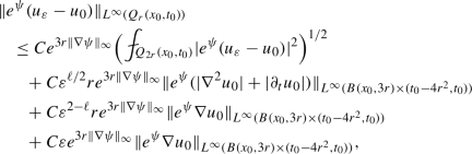
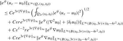
Let $w_{\varepsilon ,\delta }$ be defined by (4.8). By Lemma 4.3, we have $(\partial _t +{\mathcal {L}}_\varepsilon )w_{\varepsilon ,\delta }=\varepsilon \text {div}(F_{\varepsilon ,\delta })$ in $Q_{2r}(x_0,t_0)$. It follows from Theorem 3.1 that

where $p>d+2$. This gives

where we have used the boundedness of $\chi ^{\infty }$, ${\mathcal {B}}$ and $\nabla {\mathfrak {B}}$ in Lemmas 2.1, 2.4 and 2.2, respectively. Using $|\psi (x)-\psi (y)|\le 2r\Vert \nabla \psi \Vert _{\infty }$ for $x,y\in B(x_0,2r)$, we obtain

By setting $\delta =\varepsilon ^{\ell /2}$, and using the assumption $\varepsilon ^{\ell /2}\le r$ and Theorem 4.1, we derive (5.8) immediately.

The proof of (5.9) is completely parallel by using Lemma 4.4 and the estimates of $\chi ^{0}$, $\Phi$, and $\nabla \Upsilon$. We therefore omit the details for concision. $\square$

6 Proof of the main results

We are now ready to provide the proofs of Theorems 1.1 to 1.3.

Proof of Theorem 1.1

We follow the scheme of [9]. For fixed $x_0,y_0\in {\mathbb {R}}^{d}$ and $s_0<t_0$, it suffices to consider the case $\varepsilon +\varepsilon ^{\ell /2}<r= \sqrt{t_0-s_0} /100$, since otherwise the estimate (1.8) follows directly from (1.7). For $f\in C_{0}^{\infty }(Q_r(y_0,s_0) )$, let

$$\begin{aligned}&u_0(x,t)=\int _{-\infty }^{t}\int _{{\mathbb {R}}^{d}}\Gamma _0(x,t;y,s)f(y,s)e^{-\psi (y)}dyds,\nonumber \\&u_\varepsilon (x,t)=\int _{-\infty }^{t}\int _{{\mathbb {R}}^{d}}\Gamma _\varepsilon (x,t;y,s)f(y,s)e^{-\psi (y)}dyds. \end{aligned}$$

(6.1)

Then $(\partial _t+{\mathcal {L}}_{0})u_0=(\partial _t+{\mathcal {L}}_{\varepsilon })u_\varepsilon =e^{-\psi }f$ in ${\mathbb {R}}^{d+1}$ and $u_\varepsilon (x,t)=u_0(x,t)=0$ if $t\le s_0-r^{2}$.

We first consider the case $0<\ell <2$. Let $w_{\varepsilon ,\delta }$ be defined by (4.8) with $\delta =\varepsilon ^{\ell /2}$. It follows from (5.2), (5.3) and (5.6) that

$$\begin{aligned}&\int _{{\mathbb {R}}^{d}}|w_{\varepsilon ,\delta }(x,t)|^{2}e^{2\psi (x)}dx\nonumber \\&\quad \le C\varepsilon ^{\ell } e^{2\varepsilon ^{\ell /2}\Vert \nabla \psi \Vert _{\infty }+2\kappa (t-s_0+r^2)\Vert \nabla \psi \Vert ^{2}_{\infty }}\int _{s_0-r^{2}}^{t} \int _{{\mathbb {R}}^{d}} |f|^{2}dxds\nonumber \\&\quad \quad +C(t-s_0+r^2)\varepsilon ^{4-2\ell } e^{2\varepsilon ^{\ell /2} \Vert \nabla \psi \Vert _{\infty }+2\kappa (t-s_0+r^2)\Vert \nabla \psi \Vert ^{2}_{\infty }}\int _{s_0-r^{2}}^{t}\int _{{\mathbb {R}}^{d}} |f|^{2}dxds \end{aligned}$$

(6.2)

for any $t>s_0-r^2$. By (5.8) and the definition of $w_{\varepsilon ,\delta }$, we obtain that

(6.3)

Since $f\in C_{0}^{\infty }(Q_r(y_0,s_0) )$, (1.5) implies that

for any $x\in B(x_0,3r)$ and $|t-t_0|\le 4r^2$, where $\kappa >0$ depends only on $\mu$. Therefore, by taking (6.2) into (6.3) we deduce that

By duality we find that for any $(x,t)\in Q_r(x_0,t_0)$,

(6.4)

Let ${\widetilde{A}}={\widetilde{A}}(z,\tau )=A^{*}(z,-\tau )$ and $\widetilde{{\mathcal {L}}}_\varepsilon =-\text {div}({\widetilde{A}}\nabla )$. Let $v_{\varepsilon }(y,s)=\Gamma _{\varepsilon }(x_0,t_0;y,-s)$ and $v_{0}(y,s)=\Gamma _{0}(x_0,t_0;y,-s)$. Then

$$\begin{aligned} (\partial _t +\widetilde{{\mathcal {L}}}_\varepsilon )v_\varepsilon =(\partial _t +\widetilde{{\mathcal {L}}}_0)v_0=0 \quad \text {in } B(y_0,3r)\times (-s_0-4r^2,-s_0), \end{aligned}$$

where $\partial _{t}+\widetilde{{\mathcal {L}}}_0$ be the homogenized operator of $\partial _{t}+\widetilde{{\mathcal {L}}}_{\varepsilon }$. Since ${\widetilde{A}}$ satisfies the the same conditions as $A(z,\tau ),$ we apply Theorem 5.2 with $\psi$ replaced by $-\psi$ to obtain that

(6.5)

where we have used (1.5) for the third step and (6.4) for the last step.

Finally, to derive (1.8) we follow the ideas of [2, 11] (see also [9]) to set $\psi (y)=\gamma \psi _0(|y-y_0|)$ with $\psi _{0}(\rho )=\rho$ if $\rho \le |x_0-y_0|$ and $\psi _{0}(\rho )=|x_0-y_0|$ if $\rho >|x_0-y_0|,$ where $\gamma \ge 0$ is to be determined later. Note that $\Vert \nabla \psi \Vert _{\infty }=\gamma$ and $\psi (x_0)-\psi (y_0)=\gamma |x_0-y_0|$. By (6.5), we have

$$\begin{aligned}&|\Gamma _\varepsilon (x_0,t_0;y,s)-\Gamma _0(x_0,t_0;y,s))|\\&\quad \le C(\varepsilon ^{\ell /2}r^{-d-1} +\varepsilon ^{2-\ell }r^{-d}) e^{-\gamma |x_0-y_0|}e^{c_0(\gamma \sqrt{t_0-s_0}+(t_0-s_0)\gamma ^2)}\\&\quad \quad +C\varepsilon ^{\ell /2} r^{-d-1}e^{-\gamma |x_0-y_0|}e^{c_0(\sqrt{t_0-s_0}+|x_0-y_0|)\gamma }\exp \Big \{-\frac{\kappa |x_0-y_0|^2}{t_0-s_0}\Big \} \\&\quad \quad +C\varepsilon ^{2-\ell }r^{-d}e^{-\gamma |x_0-y_0|}e^{c_0(\sqrt{t_0-s_0}+|x_0-y_0|)\gamma }\exp \Big \{-\frac{\kappa |x_0-y_0|^2}{t_0-s_0}\Big \}, \end{aligned}$$

where $c_0$ depends at most on $\mu$. If $|x_0-y_0|\le 2c_0\sqrt{t_0-s_0}$, we choose $\gamma =0$. As a result,

$$\begin{aligned} |\Gamma _\varepsilon (x_0,t_0;y,s)-\Gamma _0(x_0,t_0;y,s))|&\le C \varepsilon ^{\ell /2} (t_0-s_0)^{\frac{-d-1}{2}} \exp \Big \{-\frac{\kappa |x_0-y_0|^2}{t_0-s_0}\Big \} \\&\quad +C\varepsilon ^{2-\ell }(t_0-s_0)^{-\frac{d}{2}}\exp \Big \{-\frac{\kappa |x_0-y_0|^2}{t_0-s_0}\Big \}. \end{aligned}$$

If $|x_0-y_0|> 2c_0\sqrt{t_0-s_0}$, we choose $\gamma =\sigma |x_0-y_0|/(t_0-s_0)$ with $\sigma \le \min \{\frac{1}{4}c_0^{-1}, 1/2(c_0+1/2)^{-1}\kappa \}$. As a result, we get

$$\begin{aligned} -\gamma |x_0-y_0|+c_0\gamma \sqrt{t_0-s_0}+c_0(t_0-s_0)\gamma ^2 \le \frac{-\sigma |x_0-y_0|^{2}}{4(t_0-s_0)}, \end{aligned}$$

and

$$\begin{aligned} c_0\gamma |x_0-y_0|+c_0\gamma \sqrt{t_0-s_0}-\frac{\kappa |x_0-y_0|^{2}}{t_0-s_0}&\le \big \{\frac{1}{2}\sigma +c_0\sigma -\kappa \big \}\frac{|x_0-y_0|^{2}}{t_0-s_0}\\&\le \frac{-\kappa |x_0-y_0|^{2}}{2(t_0-s_0)}. \end{aligned}$$

Recall that $r= \sqrt{t_0-s_0}/100$. We have thus proved that

$$\begin{aligned} |\Gamma _\varepsilon (x_0,t_0;y,s)-\Gamma _0(x_0,t_0;y,s))|&\le C \varepsilon ^{\ell /2} (t_0-s_0)^{\frac{-d-1}{2}} \exp \Big \{-\frac{\kappa _1|x_0-y_0|^2}{t_0-s_0}\Big \} \\&\quad +C\varepsilon ^{2-\ell }(t_0-s_0)^{-\frac{d}{2}}\exp \Big \{-\frac{\kappa _1|x_0-y_0|^2}{t_0-s_0}\Big \}. \end{aligned}$$

This gives the estimate (1.8) for $0<\ell <2$.

Next we consider the case $2<\ell <\infty$. Let ${\widetilde{w}}_{\varepsilon }$ be defined by (4.9). By (5.2), (5.3) and (5.7),

$$\begin{aligned}&\int _{{\mathbb {R}}^{d}}|{\widetilde{w}}_{\varepsilon }(x,t)|^{2}e^{2\psi (x)}dx\\&\quad \le C\varepsilon ^2 e^{2\varepsilon \Vert \nabla \psi \Vert _{\infty }+2\kappa (t-s_0+r^2)\Vert \nabla \psi \Vert ^{2}_{\infty }}\int _{s_0-r^2}^{t} \int _{{\mathbb {R}}^{d}}|f|^{2}dxdt\\&\quad \quad +C(t-s_0+r^2)\varepsilon ^{2\ell -4} e^{2\varepsilon \Vert \nabla \psi \Vert _{\infty }+2\kappa (t-s_0+r^2)\Vert \nabla \psi \Vert ^{2}_{\infty }}\int _{s_0-r^2}^{t}\int _{{\mathbb {R}}^{d}}|f|^{2}dxdt \end{aligned}$$

for any $t>s_0$. By using (1.5) and (5.9) we can deduce that

This, by duality, implies that

(6.6)

for any $(x,t)\in Q_r(x_0,t_0)$. Then we perform the same argument as in the case $0<\ell <2$ to consider the dual operators and chose proper function $\psi$ and finally to deduce that

$$\begin{aligned} |\Gamma _\varepsilon (x_0,t_0;y,s)-\Gamma _0(x_0,t_0;y,s))|&\le C \varepsilon (t_0-s_0)^{\frac{-d-1}{2}} \exp \Big \{-\frac{\kappa _1|x_0-y_0|^2}{t_0-s_0}\Big \} \\&\quad +C\varepsilon ^{\ell -2}(t_0-s_0)^{-\frac{d}{2}}\exp \Big \{-\frac{\kappa _1|x_0-y_0|^2}{t_0-s_0}\Big \}, \end{aligned}$$

which is exactly (1.8) in the case $2<\ell <\infty$. The proof is complete. $\square$

To prove Theorem 1.2, we shall use the following Lipschitz estimate.

Theorem 6.1

Assume that A satisfies conditions (1.2), (1.3) and (1.11). We further assume that $\Vert \partial _\tau A\Vert _{\infty }<\infty$ if $0<\ell <2$, and $\Vert \nabla ^2 A\Vert _{C^{\theta ,0} }<\infty$ if $2<\ell <\infty$. Suppose that $(\partial _t +{\mathcal {L}}_\varepsilon )u_\varepsilon =(\partial _t +{\mathcal {L}}_0)u_0$ in $Q_{2r}(x_0,t_0)$ for some $(x_0,t_0)\in {\mathbb {R}}^{d+1}$ and $\varepsilon +\varepsilon ^{\ell /2}\le r<\infty$.

• For the case $0<\ell <2$, we have

  

  (6.7)

  where C depends on $d, m, \mu$, $(h,\theta )$ in (1.11), and $\Vert \partial _\tau A\Vert _{C^{\theta ,0}}$

• For the case $2<\ell <\infty$, we have

  

  (6.8)

where C depends on $d, m, \mu$, $(h,\theta )$ in (1.11) and $\Vert \nabla ^2 A\Vert _{C^{\theta ,0}}$.

Proof

For the case $0<\ell <2$, we define

$$\begin{aligned} w_{\varepsilon }(x,t)&= u_{\varepsilon }(x,t)-u_{0}(x,t)-\varepsilon \chi ^{\infty }(x/\varepsilon ,t/\varepsilon ^{\ell })\nabla u_0(x,t)\\&\quad -\varepsilon ^{\ell }{\mathcal {B}}(t/\varepsilon ^{\ell })\nabla ^{2} u_0(x,t)-\varepsilon ^{2}\nabla {\mathfrak {B}}(x/\varepsilon ,t/\varepsilon ^{\ell })\nabla ^{2} u_0(x,t). \end{aligned}$$

By Lemma 4.3, we have $(\partial _t +{\mathcal {L}}_\varepsilon )w_{\varepsilon }=\varepsilon \text {div}(F_{\varepsilon })$ in $Q_{2r}(x_0,t_0)$, where $F_{\varepsilon }$ is defined by (4.11) with $S_{\delta }$ replaced by the identity operator. Let $\varphi \in C_{0}^{\infty }({\mathbb {R}}^{d+1})$ such that $0\le \varphi \le 1$ and

$$\begin{aligned} \begin{aligned}&\varphi =1\quad \text {in} \quad Q_{3r/2}(x_0,t_0), \quad \varphi =0 \quad \text { if } |x-x_0|\ge \frac{7}{4}r \text { or } t<t_0-\Big (\frac{7}{4}r\Big )^{2},\\&|\nabla \varphi |\le Cr^{-1}, \quad |\nabla ^{2}\varphi |+|\partial _t \varphi |\le Cr^{-2}. \end{aligned} \end{aligned}$$

(6.9)

Note that

$$\begin{aligned} (\partial _t +{\mathcal {L}}_\varepsilon )(\varphi w_{\varepsilon })&=(\partial _t\varphi )w_{\varepsilon }+\text {div}(\varepsilon \varphi F_{\varepsilon } -A^{\varepsilon } \nabla \varphi w_{\varepsilon } )- (\varepsilon F_{\varepsilon } +A^{\varepsilon }\nabla w_{\varepsilon }) \nabla \varphi . \end{aligned}$$

For any $(x,t)\in Q_{r}(x_0,t_0)$, we have

$$\begin{aligned} w_{\varepsilon }(x,t)&=\int _{-\infty }^{t}\int _{{\mathbb {R}}^{d}}\Gamma _\varepsilon (x,t;y,s) \big \{(\partial _s\varphi )w_{\varepsilon }-\varepsilon F_{\varepsilon }(\nabla \varphi )-A^{\varepsilon }\nabla w_{\varepsilon }(\nabla \varphi )\big \}dyds\\&\quad -\int _{-\infty }^{t}\int _{{\mathbb {R}}^{d}}\nabla _y\Gamma _\varepsilon (x,t;y,s) \big \{\varepsilon \varphi F_{\varepsilon }-A^{\varepsilon }(\nabla \varphi ) w_{\varepsilon }\big \}dyds\\&\doteq I_1+I_2, \end{aligned}$$

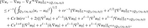
where $I_2=-\varepsilon \int _{-\infty }^{t}\int _{{\mathbb {R}}^{d}}\nabla _y\Gamma _\varepsilon (x,t;y,s) \varphi (y,s) F_\varepsilon (y,s)dyds$. By Theorem 3.3, we deduce that

where we have used Caccioppoli’s inequality for the third step. By the boundedness of $\phi$, $\nabla {\mathfrak {B}}, \nabla ^{2}{\mathfrak {B}}$ and $\partial _{\tau }\nabla {\mathfrak {B}}$ (see Lemmas 2.3 and 2.2, and Remark 2.2), we know that

$$\begin{aligned} |F_\varepsilon |\le C\big \{ |\nabla ^{2}u_0 |+(\varepsilon ^{\ell -1}+\varepsilon )|\partial _{t}\nabla u_0|+(\varepsilon +\varepsilon ^{\ell -1})|\nabla ^{3}u_0 |+\varepsilon ^{1-\ell }|\nabla u_0 |\big \}, \end{aligned}$$

(6.10)

which implies that $\Vert \nabla I_1\Vert _{L^{\infty }(Q_{r}(x_0,t_0))}$ can be bounded by the right-hand side of (6.7).

To estimate $I_2$, we note that

$$\begin{aligned} I_2(x,t)&=-\varepsilon \int _{-\infty }^{t}\int _{{\mathbb {R}}^{d}}\nabla _y\{\Gamma _\varepsilon (x,t;y,s)\varphi (y,s)\} ( F_\varepsilon (y,s)- F_\varepsilon (x,s))dyds\\&\quad +\varepsilon \int _{-\infty }^{t}\int _{{\mathbb {R}}^{d}}\Gamma _\varepsilon (x,t;y,s)\nabla _y\varphi (y,s) F_\varepsilon (y,s)dyds. \end{aligned}$$

Then for any $(x,t)\in Q_{r}(x_0,t_0)$,

In view of (6.10) and the regularity of $\phi , {\mathfrak {B}}$, we obtain that

$$\begin{aligned}&|\nabla I_2(x,t)| \\&\quad \le C\varepsilon \ln (\varepsilon ^{-1}r+2) \Vert |\nabla ^{2}u_0 |+\varepsilon ^{\ell -1}|\partial _{t}\nabla u_0|+\varepsilon ^{\ell -1}|\nabla ^{3}u_0 |+\varepsilon ^{1-\ell }|\nabla u_0 | \Vert _{L^{\infty }(Q_{2r}(x_0,t_0))}\\&\quad \quad +C\varepsilon ^{1+\theta } \Vert |\nabla ^{2}u_0 |+\varepsilon ^{\ell -1}|\partial _{t}\nabla u_0|+\varepsilon ^{\ell -1}|\nabla ^{3}u_0 | +\varepsilon ^{1-\ell }|\nabla u_0 | \Vert _{C^{\theta ,0}(Q_{2r}(x_0,t_0))}. \end{aligned}$$

Thus $\Vert \nabla I_2\Vert _{L^{\infty }(Q_{r}(x_0,t_0))}$ is bounded by the right-hand side of (6.7). Since

$$\begin{aligned} \Vert \nabla w_{\varepsilon }-\{ \nabla u_{\varepsilon }-\nabla u_{0}-(\nabla \chi ^{\infty })^{\varepsilon }\nabla u_0\} \Vert _{L^{\infty }(Q_{r}(x_0,t_0))} \le \varepsilon \Vert |\nabla ^{2}u_0|+\varepsilon ^{\ell -1}|\nabla ^{3}u_0|\Vert _{L^{\infty }(Q_{r}(x_0,t_0))}, \end{aligned}$$

one gets (6.7) immediately.

For the case $2<\ell <\infty$, we consider the function

$$\begin{aligned} {\widetilde{w}}_{\varepsilon }(x,t)&= u_{\varepsilon }(x,t)-u_{0}(x,t)-\varepsilon \chi ^{0}(x/\varepsilon )\nabla u_0(x,t)-\varepsilon ^{\ell -1}\nabla \Phi (x/\varepsilon , t/\varepsilon ^{\ell })\nabla u_0(x,t)\\&\quad -\varepsilon ^{\ell }\Phi (x/\varepsilon , t/\varepsilon ^{\ell })\nabla ^{2} u_0(x,t)-\varepsilon ^{2}\nabla \Upsilon (x/\varepsilon ) \nabla ^{2} u_0(x,t). \end{aligned}$$

By performing similar analysis as above, it is not difficult to derive (6.8). Let us omit the details. $\square$

Proof of Theorem 1.2

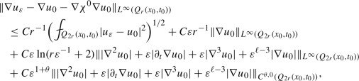
For fixed $x_0,y_0\in {\mathbb {R}}^{d}$ and $s_0<t_0$, it suffices to consider the case $\varepsilon +\varepsilon ^{\ell /2}<r=(t_0-s_0)^{1/2}/100$, since otherwise the estimate follows directly from (3.5). Note that $(\partial _t +{\mathcal {L}}_\varepsilon )u_\varepsilon =(\partial _t +{\mathcal {L}}_0)u_0=0$ in $Q_{4r}(x_0,t_0).$ We apply Theorem 6.1 to the functions $u_{\varepsilon }(x,t)=\Gamma _{\varepsilon }(x,t;y_0,s_0)$ and $u_{0}(x,t)=\Gamma _{0}(x,t;y_0,s_0)$ in $Q_{2r}(x_0,t_0)$. For the case $0<\ell <2$, it follows from (6.7) that

Since $\varepsilon ^{\ell /2}\le r$, by (1.5) and (1.8), we deduce that

$$\begin{aligned}&\big |\nabla _{x}\Gamma _\varepsilon (x,t;y,s)-\nabla _{x}\Gamma _0(x,t;y,s)-\nabla \chi ^{\infty }(x/\varepsilon ,t/\varepsilon ^{\ell }) \nabla _{x}\Gamma _0(x,t;y,s)\big |\\&\quad \le \frac{C}{(t-s)^{\frac{d+2}{2}}}\ln (2+\sqrt{t-s}/\varepsilon )\exp \Big \{-\frac{\kappa |x-y|^2}{t-s}\Big \} \cdot \big (\varepsilon ^{\ell /2} + \varepsilon ^{2-\ell }\sqrt{t-s}\big ). \end{aligned}$$

For the case $2<\ell <\infty$, we use (1.5) and (1.8) to bound the right-hand side of (6.8) to get the desired estimate. The proof is complete. $\square$

Proof of Theorem 1.3

For fixed $x_0,y_0\in {\mathbb {R}}^{d}$ and $s_0<t_0$, we may assume that $\varepsilon +\varepsilon ^{\ell /2}<r=(t_0-s_0)^{1/2}/100$. For otherwise, the estimate (1.15) follows directly from (3.6). For fixed $1\le j\le d, 1\le \beta \le m$, let

$$\begin{aligned}&u^{\alpha }_{\varepsilon } (x,t)=\frac{\partial }{\partial y_j}\{\Gamma ^{\alpha \beta }_\varepsilon \}(x,t;y_0,s_0),\\&u^{\alpha }_{0} (x,t)=\frac{\partial }{\partial y_k } \{\Gamma _0^{\alpha \zeta }\}(x,t;y,s) \frac{\partial }{\partial y_j}\big (\delta ^{\beta \zeta }y_k+ \varepsilon {\widetilde{\chi }}_k^{\beta \zeta }(y/\varepsilon ,-s/\varepsilon ^\ell \big ), \end{aligned}$$

where ${\widetilde{\chi }}_j^{\alpha \gamma }(y/\varepsilon ,-s/\varepsilon ^\ell \big )$ is the corrector of $\partial _t +\widetilde{{\mathcal {L}}}_\varepsilon$. Note that $(\partial _t +{\mathcal {L}}_\varepsilon )u_\varepsilon =(\partial _t +{\mathcal {L}}_0)u_0=0$ in $Q_{4r}(x_0,t_0).$ We can apply Theorem 6.1 to $u_\varepsilon =(u^{\alpha }_{\varepsilon } )$ and $u_0=(u^{\alpha }_{0} )$ in $Q_{2r}(x_0,t_0)$, and then use (1.5) as well as (1.14) to derive the desired estimate. $\square$

References

Bensoussan, A., Lions, J.L., Papanicolaou, G.: Asymptotic analysis for periodic structures, vol. 5, North-Holland Publishing Company Amsterdam (1978)
Cho, S., Dong, H., Kim, S.: On the Green’s matrices of strongly parabolic systems of second order. Indiana Univ. Math. J. 57(4), 1633–1677 (2008)
Davies, E.B.: Explicit constants for Gaussian upper bounds on heat kernels. Am. J. Math. 109(2), 319–333 (1987)
Davies, E.B.: Heat kernel bounds for second order elliptic operators on Riemannian manifolds. Am. J. Math. 109(3), 545–569 (1987)
Fabes, E.B., Stroock, D.W.: A new proof of Moser’s parabolic Harnack inequality using the old ideas of Nash. Arch. Ration. Mech. Anal. 96(4), 327–338 (1986)
Geng, J., Niu, W.: Homogenization of locally periodic parabolic operators with non-self-similar scales, arXiv e-prints (2021), arXiv:2103.01418
Geng, J., Shen, Z.: Uniform regularity estimates in parabolic homogenization. Indiana Univ. Math. J. 64(3), 697–733 (2015)
Geng, J., Shen, Z.: Convergence rates in parabolic homogenization with time-dependent periodic coefficients. J. Funct. Anal. 272(5), 2092–2113 (2017)
Geng, J., Shen, Z.: Asymptotic expansions of fundamental solutions in parabolic homogenization. Anal. PDE 13(1), 147–170 (2020)
Geng, J., Shen, Z.: Homogenization of parabolic equations with non-self-similar scales. Arch. Ration. Mech. Anal. 236(1), 145–188 (2020)
Hofmann, S., Kim, S.: Gaussian estimates for fundamental solutions to certain parabolic systems, Publ. Mat. 481–496 (2004)
Hofmann, S., Kim, S.: The Green function estimates for strongly elliptic systems of second order. Manuscr. Math. 124(2), 139–172 (2007)
Kenig, C.E., Lin, F., Shen, Z.: Periodic homogenization of Green and Neumann functions. Comm. Pure Appl. Math. 67(8), 1219–1262 (2014)
Meshkova, Yu.M., Suslina, T.A.: Homogenization of initial boundary value problems for parabolic systems with periodic coefficients. Appl. Anal. 95(8), 1736–1775 (2016)
Nash, J.: Continuity of solutions of parabolic and elliptic equations. Am. J. Math. 80, 931–954 (1958)
Niu, W.: Reiterated homogenization of parabolic systems with several spatial and temporal scales. J. Funct. Anal. 286(9), 110365 (2024)
Niu, W., Xu, Y.: A refined convergence result in homogenization of second order parabolic systems. J. Differ. Equs. 266(12), 8294–8319 (2019)
Niu, W., Zhuge, J.: Compactness and stable regularity in multiscale homogenization. Math. Ann. 385(3–4), 1431–1473 (2023)
Shen, Z.: Periodic homogenization of elliptic systems. Birkhäuser/Springer, Cham (2018)
Xu, Q., Zhou, S.: Quantitative estimates in homogenization of parabolic systems of elasticity in Lipschitz cylinders, arXiv:1705.01479 (2017)
Xu, Y.: Convergence rates in homogenization of parabolic systems with locally periodic coefficients. J. Differ. Equs. 367(15), 1–39 (2023)
Acknowledgements
This work is supported by NNSF of China (12371106,11971031) and NSF of Anhi Province(2108085Y01). The authors would like to thank professor Zhongwei Shen for the insightful discussions on this work.
Author information
Authors and Affiliations
Corresponding author
Additional information
Publisher's Note
Springer Nature remains neutral with regard to jurisdictional claims in published maps and institutional affiliations.
Rights and permissions
Springer Nature or its licensor (e.g. a society or other partner) holds exclusive rights to this article under a publishing agreement with the author(s) or other rightsholder(s); author self-archiving of the accepted manuscript version of this article is solely governed by the terms of such publishing agreement and applicable law.
About this article
Cite this article
Meng, Q., Niu, W. Homogenization of fundamental solutions for parabolic operators involving non-self-similar scales. Annali di Matematica 203, 2357–2382 (2024). https://doi.org/10.1007/s10231-024-01446-y
Received:
Accepted:
Published:
Issue Date:
DOI: https://doi.org/10.1007/s10231-024-01446-y