Information-preserving abstractions of event data in process mining

Abstract

Process mining aims at obtaining information about processes by analysing their past executions in event logs, event streams, or databases. Discovering a process model from a finite amount of event data thereby has to correctly infer infinitely many unseen behaviours. Thereby, many process discovery techniques leverage abstractions on the finite event data to infer and preserve behavioural information of the underlying process. However, the fundamental information-preserving properties of these abstractions are not well understood yet. In this paper, we study the information-preserving properties of the “directly follows” abstraction and its limitations. We overcome these by proposing and studying two new abstractions which preserve even more information in the form of finite graphs. We then show how and characterize when process behaviour can be unambiguously recovered through characteristic footprints in these abstractions. Our characterization defines large classes of practically relevant processes covering various complex process patterns. We prove that the information and the footprints preserved in the abstractions suffice to unambiguously rediscover the exact process model from a finite event log. Furthermore, we show that all three abstractions are relevant in practice to infer process models from event logs and outline the implications on process mining techniques.

1 Introduction

Process mining comprises methods and techniques for understanding possibly unknown processes from recorded events. Input to process mining is usually an event log containing sequences of events that describe activity occurrences observed in the past. An event log is always a finite sample of the possibly infinite behaviour of the underlying process. Process discovery has the aim of learning a process model that can describe the behaviour of this unknown process [1].

Process discovery is typically studied in terms of formal languages as illustrated in Fig. 1: process S has unknown behaviour $\mathcal {L}(S)$ from which some process executions are recorded in a log $L \subseteq \mathcal {L}(S)$—a finite language over a set of activities. A process discovery algorithm then shall infer from finite L the remaining, infinite, unobserved behaviour of S and encode them in a model M, describing possible process executions as language $\mathcal {L}(M)$. Ideally, the discovered model M describes precisely the behaviour of the underlying process S, that is, $\mathcal {L}(M) = \mathcal {L}(S)$. In practice, the underlying process S is unknown, so finding the “right” model M is often seen as a pareto-optimization problem between fitness (maximize $L \cap \mathcal {L}(M)$), precision (minimize $\mathcal {L}(M) \setminus L$), generalization (maximize behaviour not seen in L but likely to occur in the future), and simplicity of M [2].

Fig. 1

Illustration of the context of process discovery with an abstraction function $\alpha$

1.1 Information preservation in process discovery

In many time-efficient discovery algorithms [3,4,5,6], a function $\alpha$ first abstracts the known behaviour seen in L into abstract behavioural information $B = \alpha (L)$ on the activities recorded in L, thereby generalizing from the sample L. Common abstractions are the “directly follows” [3] and “eventually follows” [4] relations and their variants [7], and “behavioural profiles” [8] that also include “conflict” and “concurrency”. The discovery algorithm then synthesizes a model $M = \gamma (B)$ from B using a concretization function $\gamma$, after optionally processing B [4, 9, 10], thereby interpreting information in abstraction B.

Fig. 2

Two process models in BPMN [11], (a, b), with a different language but the same directly follows abstraction (c)

This renders the abstraction central to information preservation and inference. If for two logs (two different samples) $L_x$ and $L_y$, the abstraction yields $\alpha (L_x) = \alpha (L_y)$, then any discovery algorithm using $\alpha$ will return the same model $\gamma (\alpha (L_x)) = \gamma (\alpha (L_y))$, even if $L_x$ and $L_y$ come from different processes. For example, the two different processes in Fig. 2a, b may yield logs $L_{1} = \{ \langle a, b, c \rangle , \langle a, c, b\rangle \}$ and $L_{2} = \{ \langle a, b, c\rangle , \langle a, c, b \rangle , \langle a, b\rangle , \langle a, c\rangle \}$ both having the same directly follows abstraction shown in Fig. 2c. The directly follows abstraction is not preserving all information of Fig. 2a, b, and any discovery algorithm working with this abstraction alone cannot distinguish these logs.

Beyond event logs, stream process discovery techniques require information-preserving abstraction functions to retain information from event streams in a memory-efficient representation [12], and event databases use indexes based on abstractions [13] to efficiently discover models from very large event data sets [14]. This importance of $\alpha$ gives rise to two questions:

• When does $\alpha$ extract the “right” behavioural information about the underlying process S so that $\gamma$ can use this information to obtain the “right” model, M, with $\mathcal {L}(S) = \mathcal {L}(M)$?

• What information from a log has to be used and stored in a finite abstraction $\alpha$ to allow inferring the “right” model M?

1.2 State of the art

Although considerable progress has been made in recent years by using different abstraction and concretization functions in process discovery, more complex behaviour can still not be accurately discovered from event data [10, 15]. At the same time, the inherent information-preserving properties of the used abstractions have received considerable less attention. That is, the class of models that can be (re-)discovered has been precisely characterized for specific algorithms [3, 16,17,18,19,20,21,22]; however, a systematic study into the information preserved by the abstractions that these algorithms use has not been performed.

Information preservation and recovery for behavioural profiles independent of the alpha-algorithm are only known for acyclic processes, while behavioural profiles cannot preserve information of regular languages in general [8]. Information-preserving “footprints” of directly follows abstraction have been studied [5, 23] and used in multiple discovery algorithms [5, 6] for basic process operators. No existing study considers information preservation in abstractions for practically relevant and frequent process patterns such as unobservable skip paths, interleaving or the inclusive gateways of Fig. 2b.

1.3 Contribution

In this paper, we study how and under which circumstances event data abstractions preserve behavioural information in a way that allows to unambiguously recover basic and complex process patterns for process discovery. Specifically, we consider sequence, exclusive choice (split/join), structured loops, concurrency (split/join), critical section and inclusive choice (split/join), and unobservable paths for skipping [24]. The last three patterns have not been studied before systematically in process mining.

In Sect. 2, we expose the problem in more detail against related work and we contribute a framework to systematically investigate whether for a specific class C of languages (that are generated by process models having a particular set of operators), we can define an abstraction function $\alpha$ that can abstract any language to a finite representation and is injective: $\alpha (L_1) = \alpha (L_2)$ implies $L_1 = L_2$ (for languages $L_1$ and $L_2$), or $\alpha (\mathcal {L}(M_1)) = \alpha (\mathcal {L}(M_2))$ implies $\mathcal {L}(M_1) = \mathcal {L}(M_2)$. In these cases, discovering $\gamma (\alpha (L_1)) = \gamma (\alpha (L_2))$ is correct. Central to our proof is the definition of footprints that allow to precisely recover behavioural information from an abstraction. As the problem has no general solution, even on regular languages [8], we restrict ourselves to languages that can be described syntactically by the relevant subclass of block-structured process models in which each activity is represented at most once (that is, no duplicate activities), which we explain in Sect. 3.

We then use our framework to consolidate previous results on the information-preserving properties and to sharply characterize the limitations of the well-known directly follows abstraction $\alpha _{\text {dfg}}$ in Sect. 5. To overcome these limitations, we then propose and study two new abstractions: the minimum self-distance abstraction and its footprints discussed in Sect. 6 preserve information about loops in the context of concurrency, and our results close a gap left in earlier works [5]. The concurrent-optional-or abstraction discussed in Sect. 7 preserves information about optional behaviour, and we are the first to show that unobservable paths for skipping and inclusive choices are preserved and can be recovered from footprints in finite abstractions of languages, and hence event logs. The operational nature of the footprints allows applying them in process discovery algorithms. We report on experiments showing the practical relevance and applicability of these information-preserving abstractions for process discovery on real-life event logs in Sect. 8. Further, we discuss practical implications of our results on process mining research, mining from streams, and index design for event databases in Sect. 9.

2 Background, problem exposition, and research framework

We first discuss existing abstractions of processes and their applications. We then work out the research problem of information preservation in behavioural abstractions and propose a framework to research this problem systematically.

2.1 Background

Behavioural abstractions of process behaviour have been studied previously, generally with the aim to obtain a finite representation structure for reasoning about and comparing process behaviours. The directly follows graph (DFG) or Transition-adjacency relations [3, 5, 25] are derived from behaviour (a language or log) and relate two activities ‘A’ and ‘B’ if and only if ‘A’ can be directly followed by ‘B’; this relation can be enriched with arc weights (based on frequency of observed behaviour) [9] or semantic information from external sources [26]. Causal footprints [27] abstract model structures to graphs where multi-edges between activities (visible process steps) represent ‘and’ (concurrent) and ‘xor’ (exclusive choice) pre- and post-dependencies between activities. Behavioural profiles (BPs)  [8] derived from behaviour or models combine DFGs and causal footprints by providing binary relations for directly-following, concurrent, and conflicting (mutually exclusive) activities. Further, binary relations between activities can be defined to preserve more subtle aspects of concurrency [28]. Principal transition sequences abstract behaviour as a truncated execution tree of the model that contains all acyclic executions and truncates repetitions and unbounded behaviour [29].

Most behavioural abstractions have been used to measure similarity between process models [30]; BPs [31] and abstraction in [26] preserve more information and allow to define a metric space in order to perform searches in process model collections. In this context also non-behaviour preserving abstractions have been studied, such as projections to “relevant” subsequences [32] and isotactics for preserving concurrency of user-defined sets of activities in true-concurrency semantics [33]. BPs have also been used to propagate changes in behaviour in process model collections to other related process models [34]. Various sets of binary relations in BPs give rise to implications between relations structured along a lattice, allowing to reason within the abstractions [23, 28]. Most process discovery techniques use BPs or DFGs in several variations to abstract and generalize behavioural information from event logs [3,4,5,6, 35].

Information preservation for BPs has been studied in various ways. van der Aalst et al. [3] characterize the rediscoverable models S where from a “complete” log $L \subseteq \mathcal {L}(S)$ the discovered model M describes the same process executions: $\mathcal {L}(M) = \mathcal {L}(S)$. Their proof (1) sufficiently characterizes the rediscoverable model structures that remain distinguished under abstraction $\alpha$ into BPs, and (2) shows that the model synthesis $\gamma$ step of the alpha-algorithm reconstructs the original model. Badouel et al. [16] also provide necessary conditions. While the alpha-algorithm preserves complex structures including non-free choice constructs, behaviours such as unobservable steps, inclusive choices or interleaving are not preserved, and information is only preserved under the absence of deviations or noise [15]. Furthermore, the characterization and proofs are tied to the alpha-algorithm and cannot be applied to other contexts and discovery algorithms. Independent of an algorithm, BPs are not expressive enough to preserve even trace equivalence for any general class of behaviour (within regular languages) [8]. BPs preserve behaviour for acyclic, unlabelled models, i.e. where each activity in the model is observable and distinct from all other activities [8, 36]. For cyclic models, only for unlabelled, free-choice workflow nets a variant of BPs including the “up-to-k” successor relation preserves trace equivalence, though k is model specific [7]; for large enough k, this resembles the eventually follows relation.

Information preservation for DFGs has been studied as rediscoverability for the Inductive Miner [5] and the alpha-algorithm [3, 16] and its variants. For instance, several variants of the alpha-algorithm have been introduced to include short loops (alpha$^+$ [17]), to include long-distance dependencies [18] (using the eventually follows relation, but only for acyclic processes), to include non-free-choice constructs (alpha$^{++}$ [19]) and to include certain types of silent transitions (alpha$^\#$ [20, 21], alpha$^{\$}$ [22]). For these algorithms, it was shown that they could obtain enough information from an event log to reliably rediscover certain constructs; however, these characterizations and proofs are tied to the specific algorithms and cannot be applied to other contexts and discovery algorithms. Information preservation in Inductive Miner [5] was proven by showing that behavioural information can be completely retrieved from the abstraction itself, in the form of footprints in the DFG, independent of a specific model synthesis algorithm, and characterizing the block-structured models for which this information is preserved in the DFG. However, these footprints allow reusing information abstraction and recovery in other (non-block-structured) contexts such as the Split Miner [6], which uses footprints from the DFG in a different way to synthesize a model, or Projected Conformance Checking [37], which uses abstractions to provide guarantees in approximative fast conformance checking measures. Other process discovery techniques might be able to obtain enough information from event logs to reconstruct a model, such as (conjectured) the ILP miner [35] and several genetic techniques [38, 39], but no insights into guarantees and limits of information preservation are available.

2.2 Problem exposition

This paper particularly addresses information-preserving capabilities of abstractions of languages in general, that hold in any application using these abstractions, rather than just a single specific algorithm. To approach the problem in an algorithm-independent setting, we generalize prior work on rediscoverability to the following sub-problems:

• RQ1 For which class $\textsc {C}$ of languages is each language Luniquely defined by its syntactic model M with $L = \mathcal {L}(M)$, i.e. $\mathcal {L}(M_1) = \mathcal {L}(M_2)$ implies $M_1 = M_2$?

• RQ2 For which class $\textsc {C}$ of languages does an abstraction $\alpha$ distinguish languages on their abstractions alone, that is, when does $\alpha (L_1) = \alpha (L_2)$ imply $L_1 = L_2$ for $L_1,L_2 \in \textsc {C}$?

• RQ3 For which class $\textsc {C}$ of languages does $\alpha$ preserve the information about the entire model syntax, i.e. when does $\alpha (\mathcal {L}(M_1)) = \alpha (\mathcal {L}(M_2))$ imply $M_1 = M_2$?

• RQ4 For which classes $\textsc {C}$ of languages and which abstractions $\alpha$ can syntactic constructs of model M be recognized in $\alpha (\mathcal {L}(M))$?

The specific objective of RQ4 is to not only ensure that an abstraction $\alpha$ can distinguish different types of behaviour, but that information about the behaviour can be recovered from the abstraction, so the abstraction can be exploited by different process discovery algorithms.

2.3 Research framework

As discussed in Sect. 1, we will answer the above questions for three different abstractions: directly follows $\alpha _{\text {dfg}}$, minimum self-distance $\alpha _{\text {msd}}$, and concurrent-optional-or $\alpha _{\text {coo}}$. Each abstraction function $\alpha _x$ returns a finite abstraction $\alpha _x(L)$ for any language L in the form of finite graphs over the alphabet $\Sigma$ of L. As RQ2 has no general answer [8], we limit our model class to a very general class of block-structured models $C_\mathcal {B}$ defined in Sect. 3. We then employ the following framework to answer RQ1–RQ4 for each abstraction:

• Using a system of sound rewriting rules on block-structured process models [40, p. 113] explained in Sect. 4, we obtain a unique syntactic normal form $NF (M)$ for each model $M\in C_\mathcal {B}$.

• We show that each abstraction $\alpha _x(L)$ of any language L of some model $M \in C_\mathcal {B}, L=\mathcal {L}(M)$ preserves not only the behaviour but also syntax of M in an implicit form: we can recover from $\alpha _x(L)$ the top-level operator of the normal form $NF (M)$ through specific characteristic features in $\alpha _x(L)$, called footprints, answering RQ4. Specifically, much of the information preserved in BPs is already contained in the more basic $\alpha _{\text {dfg}}$ from which not only sequence, choice, loops and concurrency but also interleaving (Sect. 5) can be recovered. The minimum self-distance abstraction $\alpha _{\text {msd}}$ preserves information about loops in the context of concurrency (Sect. 6) allowing to preserve information from a larger model class. The new concurrent-optional-or abstraction $\alpha _{\text {coo}}$ (Sect. 7) preserves information about unobservable skipping and inclusive choices not considered before.

• We then characterize for each abstraction $\alpha _x$ the class of models $C_x \subset C_\mathcal {B}$ for which the entire recursive structure of $M \in C_x$ is uniquely preserved in the abstraction of its language $\alpha _x(\mathcal {L}(M))$; each $C_x$ partially constrains the nesting of operators, most notably concurrency.

• As our core result, we then show that the languages $\mathcal {L}(M_1),\mathcal {L}(M_2)$ of any two models $M_1,M_2 \in C_x$ with different normal forms $NF (M_1) \ne NF (M_2)$ can always be distinguished in their finite abstractions $\alpha _x(\mathcal {L}(M_1)) \ne \alpha _x(\mathcal {L}(M_2))$ based on the footprints in $\alpha _x$. Our characterization is sharp in the sense that for any necessary condition, we provide a counterexample, answering RQ3.

• As the normal form $NF (M)$ is unique, we can then conclude RQ2: any two different languages$L_1 \ne L_2$ of any two models $L_i = \mathcal {L}(M_i), M_i \in C_x$ can always be distinguished by their finite abstractions $\alpha _x(L_1) \ne \alpha _x(L_2)$.

• We finally can answer RQ1: by RQ3 two different syntactic normal forms $NF (M_1) \ne NF (M_2)$ have different abstractions of their languages $\alpha _x(L_1) \ne \alpha _x(L_2), L_i = \mathcal {L}( NF (M_i))$ and have therefore different languages $L_1 \ne L_2 \in C_x$ (as $\alpha _x$ is a deterministic function).

3 Preliminaries

3.1 Traces, languages, partitions

A trace is a sequence of events, which are executions of activities (i.e. the process steps). The empty trace is denoted with $\epsilon$.

A language is a set of traces, and an event log is a finite set of traces. For instance, the language $L_{3} = \{\langle a, b, c \rangle , \langle a, c, b\rangle \}$ consists of two traces. For the first trace, first activity a was executed, followed by b and c. Traces can be concatenated using $\cdot$.

In this paper, we limit ourselves to regular languages, that is, languages that can be defined using the regular expression patterns sequence, exclusive choice and Kleene star.

We refer to the activities that appear in a language or event log as the alphabet$\Sigma$ of the language or event log. A partition of an alphabet consists of several sets, such that each activity of the alphabet appears in precisely one of the sets, and each activity in the sets appears in the alphabet. For instance, the alphabet of $L_{3}$ is $\{a, b, c\}$ and a partition of this alphabet is $\{\{a, b\}, \{c\}\}$.

3.2 Block-structured models

A block-structured process model can be recursively broken up into smaller pieces. These smaller pieces form a hierarchy of model constructs, that is, a tree [41].

A process tree is an abstract representation of a block-structured workflow net [1]. The leaves are either unlabelled or labelled with activities, and all other nodes are labelled with process tree operators. A process tree describes a language: the leaves describe singleton or empty languages, and an operator describes how the languages of its subtrees are to be combined. We formally define process trees recursively:

Definition 3.1

(process tree syntax) Let $\Sigma$ be an alphabet of activities, then

• activity$a \in \Sigma$ is a process tree;

• the silent activity$\tau$ ($\tau \notin \Sigma$) is a process tree;

• let $M_1 \ldots M_n$ with $n > 0$ be process trees and let $\oplus$ be a process tree operator; then, the operator node$\oplus (M_1, \ldots M_n)$ is a process tree. We also write this as

  

Each process tree describes a language: an activity describes the execution of that activity, a silent activity describes the empty trace, while an operator node describes a combination of the languages of its children. Each operator combines the languages of its children in a specific way.

Fig. 3

Recursive Petri-net translations of process trees

In this paper, we consider six process tree operators:

• 1. exclusive choice ,

• 2. sequence $\rightarrow$,

• 3. interleaved (i.e. not overlapping in time) $\leftrightarrow$,

• 4. concurrency (i.e. possibly overlapping in time) $\wedge$,

• 5. inclusive choice and

• 6. structured loop $\circlearrowleft$ (i.e. the loop body $M_1$ and alternative loop back paths $M_2 \ldots M_n$).

For instance, the language of

is $\{\langle a, b, c \rangle$, $\langle b, a, c \rangle$, $\langle b, c, a \rangle$, $\langle d, e, f \rangle$, $\langle e, f, d \rangle$, $\langle g \rangle$, $\langle h \rangle$, $\langle g, h \rangle$, $\langle h, g \rangle$, $\langle i \rangle$, $\langle i, j, i \rangle$, $\langle i, j, i, j, i \rangle$$\ldots \}$. A formal definition of these operators is given in “Appendix A”.

Each of the process tree operators can be translated to a sound block-structured workflow net, and to, for instance, a BPMN model [11]. Figure 3 provides some intuition by giving the translation of the process tree operators to (partial) Petri nets [42].

We refer to a process tree that is part of a larger process tree as a subtree of the larger tree.

4 A canonical normal form for process trees

Some process trees are structurally different but nevertheless express the same language. For instance, the process trees

and

have a different structure but the same language, consisting of the choice between a, b and c. Such trees are indistinguishable by their language, and thus also indistinguishable by any language abstraction. To take such structural differences out of the equation, we use a set of rules that, when applied, preserve the language of a tree while reducing the structural size and complexity of the tree. It does not matter which rules or in which order the rules are applied: applying the rules exhaustively always yields the same canonical normal form.

The set of rules consist of four types of rules: (1) a singularity rule, which removes operators with only a single child: $\oplus (M) \Rightarrow M$ for any process tree M and operator $\oplus$ (except $\circlearrowleft$); (2) associativity rules, which remove nested operators of the same type, such as $\circlearrowleft ( \circlearrowleft ( M, \ldots _1 ), \ldots _2 ) \Rightarrow \,\circlearrowleft ( M, \ldots _1, \ldots _2 )$; (3) $\tau$-reduction rules, which remove superfluous $\tau$s, such as $\wedge (\ldots , M, \tau ) \Rightarrow \wedge (\ldots , M)$; and (4) rules that establish the relation between concurrency and other operators, such as $\leftrightarrow (M_1, \ldots M_n) \Rightarrow \wedge (M_1, \ldots M_n)$ with $\forall _{1 \leqslant i \leqslant n, t \in \mathcal {L}(M_i)}~ |t| \leqslant 1$.

The set of rules is terminating, that is, to any process tree only a finite number of rules can be applied sequentially; the set is locally confluent, that is, if two rules are applicable to a single tree, yielding trees A and B, then it is possible to reduce A and B to a common tree C; and by extension, the set of rules is confluent and canonical. For more details, please refer to [40, p. 118].

As a result, the rules are canonical, so in the remainder of this paper, we only need to consider process trees in canonical normal form, to which we refer as reduced process trees; a reduced process tree is a process to which the reduction rules have been applied exhaustively. This allows us to reason based on the structure of reduced trees, rather than on the behaviour of arbitrarily structured trees.

5 Preservation and recovery with directly follows graphs

In order to study the information preserved in abstractions, in this section we study the first abstraction: directly follows graphs. This abstraction has been well studied in context of process discovery. For instance, in the context of the alpha-algorithm, the directly follows abstraction has been shown to preserve information about a certain class of Petri nets. In this section, we show that directly follows graphs preserve even more information than previously known.

We first formally introduce the abstraction, after which we introduce characteristics of the recursive process tree operators in the abstraction: footprints. Using these footprints, we show that every two reduced process trees that are structurally different have different abstractions. That is, we show that if two trees have the same directly follows abstraction, then there cannot be a structural difference between the two trees. For subsequent abstractions in this paper, which get more involved, we will use a similar proof strategy.

We first introduce the abstraction. Second, we introduce the footprints of the recursive process tree operators in this abstraction. Third, we introduce a class of recursively defined languages and show that this class is tight, that is, structurally different trees outside this class might yield the same abstraction. Finally, we show that different normal forms within the class have different abstractions (and hence languages), thereby using the research framework of Sect. 2.

5.1 Directly follows graphs

A directly follows graph abstracts from a language by only expressing which activities (the nodes of the graph) are followed directly by which activities in a trace in the language. Furthermore, a directly follows graph expresses the activities with which traces start or end in the language, and whether the language contains the empty trace.

Definition 5.1

(directly follows graph) Let $\Sigma$ be an alphabet and let L be a language over $\Sigma$ such that $\epsilon \notin \Sigma$. Then, the directly follows graph$\alpha _{\text {dfg}}$ of L consists of:

$$\begin{aligned} \alpha _{\text {dfg}}(a, b) \Leftrightarrow {}&\exists _{t \in L}~ t = \langle \ldots a, b, \ldots \rangle \\ a \in {{\,\mathrm{Start}\,}}(\alpha _{\text {dfg}}) \Leftrightarrow {}&\exists _{t \in L}~ t = \langle a, \ldots \rangle \\ a \in {{\,\mathrm{End}\,}}(\alpha _{\text {dfg}}) \Leftrightarrow {}&\exists _{t \in L}~ t = \langle \ldots , a \rangle \\ \epsilon \in \alpha _{\text {dfg}}\Leftrightarrow {}&\exists _{t \in L}~ t = \epsilon \end{aligned}$$

For a directly follows graph $\alpha _{\text {dfg}}$, $\Sigma (\alpha _{\text {dfg}})$ denotes the alphabet of activities, i.e. the nodes of $\alpha _{\text {dfg}}$.

For instance, let $L_{4} = \{ \langle a, b, c \rangle , \langle a, c, b \rangle , \epsilon \}$ be a language. Then, the directly follows graph of $L_{4}$ consists of the edges $\alpha _{\text {dfg}}(a, b)$, $\alpha _{\text {dfg}}(b, c)$, $\alpha _{\text {dfg}}(a, c)$, $\alpha _{\text {dfg}}(c, b)$. The start activity is a, the end activities are b and c and the directly follows graph contains $\epsilon$. A graphic representation of this directly follows graph is shown in Fig. 4.

Fig. 4

An example of a directly follows graph: $\alpha _{\text {dfg}}(L_{4})$

5.2 Footprints

Each process tree operator has a particular characteristic in a directly follows graph, a footprint. We will use footprints in our uniqueness proofs to show differences between trees: if one tree contains a particular footprint and another one does not, the languages of these trees must be different. Furthermore, process discovery algorithms can use footprints to infer syntactic constructs that capture the abstracted behaviour.

In this section, we introduce these characteristics and show that process tree operators exhibit them.

A cut is a tuple $(\oplus , \Sigma _1, \ldots \Sigma _m)$, such that $\oplus$ is a process tree operator and $\Sigma _1 \ldots \Sigma _m$ are sets of activities. A cut is non-trivial if $m > 1$ and no $\Sigma _i$ is empty.

Definition 5.2

(directly follows footprints) Let $\alpha _{\text {dfg}}$ be a directly follows relation and let $c = (\oplus , \Sigma _1, \ldots \Sigma _n)$ be a cut, consisting of a process tree operator and a partition of activities with parts $\Sigma _1 \ldots \Sigma _n$ such that $\Sigma (\alpha _{\text {dfg}}) = \bigcup _{1 \leqslant i \leqslant n} \Sigma _i$ and $\forall _{1 \leqslant i < j \leqslant n}~ \Sigma _i \cap \Sigma _j = \emptyset$.

• Exclusive choice. c is an exclusive choice cut in $\alpha _{\text {dfg}}$ if and

x.1:

No part is connected to any other part:

• Sequential. c is a sequence cut in $\alpha _{\text {dfg}}$ if $\oplus = \rightarrow$ and

s.1:

Each node in a part is indirectly and only connected to all nodes in the parts “after” it:

• Interleaved. c is an interleaved cut in $\alpha _{\text {dfg}}$ if $\oplus = \leftrightarrow$ and

i.1:

Between parts, all and only connections exist from an end to a start activity:

• Concurrent. c is a concurrent cut in $\alpha _{\text {dfg}}$ if $\oplus = \wedge$ and

c.1:

Each part contains a start and an end activity.

c.2:

All parts are fully interconnected.

• Loop. c is a loop cut in $\alpha _{\text {dfg}}$ if $\oplus \,=\,\circlearrowleft$ and

l.1:

All start and end activities are in the body (i.e. the first) part.

l.2:

Only start/end activities in the body part have connections from/to other parts.

l.3:

Redo parts have no connections to other redo parts.

l.4:

If an activity from a redo part has a connection to/from the body part, then it has connections to/from all start/end activities.

A formal definition is included in “Appendix B.1”.

For instance, consider the directly follows graph of $L_{4}$ shown in Fig. 4: in this graph, the cut $(\rightarrow , \{a\}, \{b, c\})$ is a $\rightarrow$-cut.

Inspecting the semantics of the process tree operators (Definition A.1), it follows that in the directly follows graphs of process trees, these footprints are indeed present:

Lemma 5.1

(Directly follows footprints) Let $M = \oplus (M_1, \ldots M_m)$ be a process tree without duplicate activities, with . Then, the cut $(\oplus$, $\Sigma (M_1)$, $\ldots \Sigma (M_n))$ is a $\oplus$-cut in $\alpha _{\text {dfg}}(M)$ according to Definition 5.2.

5.3 A class of trees: $\textsc {C}_{\text {dfg}}$

Not all process trees can be distinguished using the introduced footprints. In this section, we describe the class of trees that can be distinguished by directly follows graphs: $\textsc {C}_{\text {dfg}}{}$. To illustrate that this class is tight, we give counterexamples of pairs of trees outside of $\textsc {C}_{\text {dfg}}{}$ and show that these trees cannot be distinguished using their directly follows graphs.

Definition 5.3

(Class $\textsc {C}_{\text {dfg}}$) Let $\Sigma$ be an alphabet of activities. Then, the following process trees are in $\textsc {C}_{\text {dfg}}$:

• a with $a \in \Sigma$ is in $\textsc {C}_{\text {dfg}}$

• Let $M_1 \ldots M_n$ be reduced process trees in $\textsc {C}_{\text {dfg}}$ without duplicate activities:

  $\forall _{i \in [1\ldots n], i \ne j \in [1\ldots n]}~ \Sigma (M_i) \cap \Sigma (M_j) = \emptyset$. Then,

• $\oplus (M_1, \ldots M_n)$ with is in $\textsc {C}_{\text {dfg}}$;

• $\leftrightarrow (M_1, \ldots M_n)$ is in $\textsc {C}_{\text {dfg}}$ if all:

i.1:

At least one child has disjoint start and end activities:

$\exists _{i \in [1\ldots n]}~ {{\,\mathrm{Start}\,}}(M_i) \cap {{\,\mathrm{End}\,}}(M_i) = \emptyset$;

i.2:

No child is interleaved itself:

$\forall _{i\in [1\ldots n]}~ M_i \ne \leftrightarrow (\ldots )$;

i.3:

Each concurrent child has at least one child with disjoint start and end activities:

$\forall _{i \in [1\ldots n] \wedge M_i = \wedge (M_{i_1}, \ldots M_{i_m}) }~ \exists _{j \in [1 \ldots m]}~ {{\,\mathrm{Start}\,}}(M_{i_j}) \cap {{\,\mathrm{End}\,}}(M_{i_j}) = \emptyset$

• $\circlearrowleft (M_1, \ldots M_n)$ is in $\textsc {C}_{\text {dfg}}$ if:

l.1:

the first child has disjoint start and end activities:

${{\,\mathrm{Start}\,}}(M_1) \cap {{\,\mathrm{End}\,}}(M_1) = \emptyset$.

These requirements are tight as for each requirement there exists counterexamples of the following form: two process trees whose syntax violates the requirement and who have different languages but have identical directly follows graphs. Consequently, the two trees cannot be distinguished by the directly follows abstraction.

Figure 5 illustrates the counterexample for $\hbox {C}_{\mathrm{dfg}}.\hbox {l}.1$. This requirement has some similarity with the so-called short loops of the $\alpha$ algorithm [1].

The counterexamples for $\hbox {C}_{\mathrm{dfg}}.\hbox {i}.1$, $\hbox {C}_{\mathrm{dfg}}.\hbox {i}.2$ and $\hbox {C}_{\mathrm{dfg}}.\hbox {i}.3$ follow a similar reasoning and are given in “Appendix C.1”.

Trees with $\tau$ and nodes are excluded from $\textsc {C}_{\text {dfg}}$ entirely. The corresponding counterexamples for the directly follows abstraction and how to preserve information on $\tau$ and will both be discussed in Sect. 7.

Fig. 5

An example for the necessity of Requirement $\hbox {C}_{\mathrm{dfg}}.\hbox {l}.1$

A weaker requirement one could consider to replace $\hbox {C}_{\mathrm{dfg}}.\hbox {l}.1$is that at least one child of the loop should have disjoint start and end activities: $M'\,=\,\circlearrowleft (M'_1, \ldots M'_n): \exists _{1 \leqslant i \leqslant n}~ {{\,\mathrm{Start}\,}}(M'_i) \cap {{\,\mathrm{End}\,}}(M'_i) = \emptyset$. This weaker requirement would allow both $M_{7}$ and $M_{8}$ (see Fig. 6), i.e. c can be in the redo of the inner or outer $\circlearrowleft$-nodes. However, the counterexample in Fig. 6 shows that this weaker constraint is not strong enough.

Fig. 6

A counterexample that a weaker constraint, which would state that at least one child of a $\circlearrowleft$ node should have disjoint start and end activities, would not suffice to replace Requirement $\hbox {C}_{\mathrm{dfg}}.\hbox {l}.1$

5.4 Uniqueness

Now that all concepts for abstraction and recovery have been introduced, what is left is to prove for $\alpha _{\text {dfg}}$ which behaviour can be preserved. Here, we provide the lemmas and theorems according to the framework of Sect. 2 to establish the fundamental formal limits. This proof structure will be reused on the more complex abstractions later.

That is, in this section, we prove that two structurally different reduced process trees of $\textsc {C}_{\text {dfg}}$ always have different directly follows graphs. To prove this, we exploit the recursive structure of process trees: we first show that if the root operator of two process trees differs, then their directly follows graphs differ. Second, we show that if the activity partition (that is, the distribution of activities over the children of the root) of two trees differs, then their directly follows graphs differ. These two results yield that any structural difference over the entire tree will result in a different directly follows graph.

Lemma 5.2

(Operators are mutually exclusive) Take two reduced process trees of $\textsc {C}_{\text {dfg}}$$K = \oplus (K_1, \ldots K_n)$ and $M = \otimes (M_1, \ldots M_m)$ such that $\oplus \ne \otimes$. Then, $\alpha _{\text {dfg}}(K) \ne \alpha _{\text {dfg}}(M)$.

This lemma is proven by showing that for each pair of operators, there is always a difference in their directly follows graphs. For instance, the directly follows graph of a node is not connected, while all other operators make the graph connected. For a detailed proof, please refer to “Appendix D.1”.

Lemma 5.3

(Partitions are mutually exclusive) Take two reduced process trees of $\textsc {C}_{\text {dfg}}$$K = \oplus (K_1 \ldots K_n)$ and $M = \oplus (M_1 \ldots M_m)$ such that their activity partition is different: $\exists _{1 \leqslant w \leqslant \text {min}(n, m)}~ \Sigma (K_w) \ne \Sigma (M_w)$. Then, $\alpha _{\text {dfg}}(K) \ne \alpha _{\text {dfg}}(M)$.

For this proof, we assume a fixed order of children for the non-commutative operators $\rightarrow$ and $\circlearrowleft$. Then, we show, for each operator, that a difference in activity partitions leads to a difference in directly follows graphs. For a detailed proof, please refer to “Appendix D.2”.

Lemma 5.4

(Abstraction uniqueness for $\textsc {C}_{\text {dfg}}$) Take two reduced process trees of $\textsc {C}_{\text {dfg}}$K and M such that $K \ne M$. Then, $\alpha _{\text {dfg}}(K) \ne \alpha _{\text {dfg}}(M)$.

Proof

Towards contradiction, assume that there exist two reduced process trees K and M, both of $\textsc {C}_{\text {dfg}}$, such that $\alpha _{\text {dfg}}(K) = \alpha _{\text {dfg}}(M)$, but $K \ne M$. Then, there exist topmost subtrees $K'$ in K and $M'$ in M such that $\alpha _{\text {dfg}}(K') = \alpha _{\text {dfg}}(M')$ and such that $K'$, $M'$ are structurally different in their activity, operator or activity partition, i.e. either

• $K'$ or $M'$ is a $\tau$, while the other is not. Then, obviously $\alpha _{\text {dfg}}(K') \ne \alpha _{\text {dfg}}(M')$.

• $K'$ or $M'$ is a single activity while the other is not. Then, by the restrictions of $\textsc {C}_{\text {dfg}}$, $\alpha _{\text {dfg}}(K') \ne \alpha _{\text {dfg}}(M')$.

• $K' = \otimes (K'_1 \ldots K'_ n)$ and $M' = \oplus (M'_1 \ldots M'_n)$ such that $\oplus \ne \otimes$. By Lemma 5.2, $\alpha _{\text {dfg}}(K') \ne \alpha _{\text {dfg}}(M')$.

• $K' = \oplus (K'_1 \ldots K'_ n)$ and $M' = \oplus (M'_1 \ldots M'_n)$ such that the activity partition is different, i.e. there is an i such that $\Sigma (K'_i) \ne \Sigma (M'_i)$. By Lemma 5.3, $\alpha _{\text {dfg}}(K') \ne \alpha _{\text {dfg}}(M')$.

Hence, there cannot exist such K and M, and therefore, $\alpha _{\text {dfg}}(K) \ne \alpha _{\text {dfg}}(M)$. $\square$

As a language abstraction is solely derived from a language, different directly follows graphs imply different languages (the reverse not necessarily holds), we immediately conclude uniqueness:

Corollary 5.1

(Language uniqueness for $\textsc {C}_{\text {dfg}}$) There are no two different reduced process trees of $\textsc {C}_{\text {dfg}}$ with equal languages. Hence, for trees of class $\textsc {C}_{\text {dfg}}$, the normal form of Sect. 4 is uniquely defined.

Fig. 7

Example of two process trees outside of $\textsc {C}_{\text {dfg}}$ that have the same directly follows graph. In this section, we introduce the new minimum self-distance abstraction ($\alpha _{\text {msd}}$) and corresponding footprints that distinguish these trees

6 Preservation and recovery with minimum self-distance

A structure that is difficult to distinguish in directly follows graphs is the nesting of $\circlearrowleft$ and $\wedge$ operators, resembling the so-called short loops of the $\alpha$ algorithm. For instance, Fig. 7 shows an example of two process trees with such a nesting, having the same directly follows graph. In $\textsc {C}_{\text {dfg}}$, such nestings were excluded.

In this section, we introduce a new abstraction, the minimum self-distance abstraction, that distinguishes some of such nestings by considering which activities must be in between two executions of the same activity. As illustrated in Fig. 7, the minimum self-distance abstraction captures more information of process trees, enabling discovery and conformance checking algorithms to distinguish the languages of these trees.

The remainder of this section follows a strategy similar to Sect. 5: first, we introduce the language abstraction of minimum self-distance graphs. Second, we introduce adapted footprints of the recursive process tree operators in minimum self-distance graphs. Third, we characterize the extended class of recursively defined languages and show where this class is tight (conditions cannot be dropped). Fourth, we show that different trees in normal form of this class have different combinations of directly follows graphs and minimum self-distance graphs (and hence languages), using the research framework of Sect. 2.

6.1 Minimum self-distance

The minimum self-distancem of an activity is the minimum number of events in between two executions of that activity:

Definition 6.1

(Minimum self-distance) Let L be a language, and let $a, b \in \Sigma (L)$. Then,

$$\begin{aligned} m(a) = \left\{ \begin{array}{ll} {\min }_{\langle \ldots , a, \ldots _1, a, \ldots \rangle \in L} |\ldots _1| &{} \text {if } \exists _{\langle \ldots , a, \ldots _1, a, \ldots \rangle \in L}~\\ \infty &{} \text {otherwise} \end{array}\right. \end{aligned}$$

A minimum self-distance graph$\alpha _{\text {msd}}$ is a directed graph whose nodes are the activities of the alphabet $\Sigma$. An edge $\alpha _{\text {msd}}(a, b)$ in a minimum self-distance graph denotes that b is a witness of the minimum self-distance of a, i.e. activity b can appear in between two minimum-distant executions of activity a:

Definition 6.2

(Minimum self-distance graph) Let L be a language, and let $a, b \in \Sigma (L)$. Then,

$$\begin{aligned} \alpha _{\text {msd}}(a, b) \equiv \exists _{\langle \ldots , a, \ldots _1, a, \ldots \rangle \in L}~ b \in \ldots _1 \wedge |\ldots _1| = m(a) \end{aligned}$$

For a minimum self-distance graph $\alpha _{\text {msd}}$, $\Sigma (\alpha _{\text {msd}})$ denotes the alphabet of activities, i.e. the nodes of $\alpha _{\text {msd}}$.

For instance, consider the log $L_{11} = \{ \langle a, b \rangle , \langle b, a, c, a, b \rangle , \langle a, b, c, a, b, c, b, a \rangle \}$. In this log, the minimum self-distances are $m(a) = 1$, $m(b) = 1$ and $m(c) = 2$, witnessed by the subtraces $\langle a, c, a \rangle$ (for a), $\langle b, c, b \rangle$ (for b) and $\langle c, a, b, c \rangle$ (for c). Thus, the minimum self-distance relations are $\alpha _{\text {msd}}(a, c)$, $\alpha _{\text {msd}}(b, c)$, $\alpha _{\text {msd}}(c, a)$ and $\alpha _{\text {msd}}(c, b)$. Figure 8 visualizes this minimum self-distance relation as a graph.

Fig. 8

Minimum self-distance graph of $L_{11}$

6.2 Footprints

In this section, we introduce the characteristics that process tree operators leave in minimum self-distance graphs.

Definition 6.3

(minimum self-distance footprints) Let $\alpha _{\text {msd}}$ be a minimum self-distance graph and let $c = (\oplus , \Sigma _1, \ldots \Sigma _n)$ be a cut, consisting of a process tree operator and a partition of activities with parts $\Sigma _1 \ldots \Sigma _n$ such that $\Sigma (\alpha _{\text {msd}}) = \bigcup _{1 \leqslant i \leqslant n} \Sigma _i$ and $\forall _{1 \leqslant i < j \leqslant n}~ \Sigma _i \cap \Sigma _j = \emptyset$.

• Concurrent and interleaved. If $\oplus = \wedge$ or $\oplus = \leftrightarrow$, then in $\alpha _{\text {msd}}$:

ci.1:

There are no $\alpha _{\text {msd}}$ connections between parts:

• Loop. If $\oplus = \circlearrowleft$ then in $\alpha _{\text {msd}}$:

l.1:

Each activity has an outgoing edge.

l.2:

All redo activities that have a connection to a body activity have connections to the same body activities:

l.3:

All body activities that have a connection to a redo activity have connections to the same redo activities:

l.4:

No two activities from different redo children have an $\alpha _{\text {msd}}$-connection:

A formal definition is included in “Appendix B.2”.

For instance, consider the example shown in Fig. 7: the two process trees $M_{9}$ and $M_{10}$ have the same directly follows graph (Fig. 7c). However, the minimum self-distance graphs of these two trees differ (Fig. 7d, e). To exploit this difference, the footprints in both graphs differ: in $\alpha _{\text {msd}}(M_{9})$, the only footprint is $(\circlearrowleft , \{a, b\}, \{c\})$, while in $\alpha _{\text {msd}}(M_{9})$ the only footprint is $(\wedge , \{a, c\}, \{b\})$ footprint.

From the semantics of process trees, it follows that these footprints are present in minimum self-distance graphs of process trees without duplicate activities:

Lemma 6.1

(Minimum self-distance footprints) Let $M = \oplus (M_1, \ldots M_m)$ be a process tree without duplicate activities, with . Then, the cut $(\oplus$, $\Sigma (M_1)$, $\ldots \Sigma (M_n))$ is a $\oplus$-cut in $\alpha _{\text {msd}}(M)$ according to Definition 6.3.

6.3 A class of trees: $\textsc {C}_{\text {msd}}$

Using the minimum self-distance graph, we can lift a restriction of $\textsc {C}_{\text {dfg}}$ partially. In this section, we introduce the extended class of process trees $\textsc {C}_{\text {msd}}$, in which a $\circlearrowleft$-node can be a direct child of a $\wedge$-node.

Definition 6.4

(Class$\textsc {C}_{\text {msd}}$) Let $\Sigma$ be an alphabet of activities. Then, the following process trees are in $\textsc {C}_{\text {msd}}$:

• $M \in \textsc {C}_{\text {dfg}}$ is in $\textsc {C}_{\text {msd}}$;

• Let $M_1 \ldots M_n$ be reduced process trees in $\textsc {C}_{\text {msd}}$ without duplicate activities: $\forall _{i \in [1\ldots n], i \ne j \in [1\ldots n]}~ \Sigma (M_i) \cap \Sigma (M_j) = \emptyset$. Then, $\circlearrowleft (M_1, \ldots M_n)$ is in $\textsc {C}_{\text {msd}}$ if:

l.1:

the body child is not concurrent:

$M_1 \ne \wedge (\ldots )$

We neither have a proof nor a counterexample for the necessity of Requirement $\hbox {C}_{\mathrm{msd}}.\hbox {l}.1$. Figure 9 illustrates this: the two trees have a different language, an equivalent $\alpha _{\text {dfg}}$-graph (shown in Fig. 9b) but a different $\alpha _{\text {msd}}$-graph (shown in Fig 9c, d). Thus, they could be distinguished using their $\alpha _{\text {msd}}$-graph. However, the footprint (Definition 6.3) cannot distinguish these trees: both cuts $(\circlearrowleft , \{a, b, c\}, \{d\})$ and $(\circlearrowleft , \{a, c, d\}, \{b\})$ are valid in both $\alpha _{\text {msd}}$-graphs, where $(\circlearrowleft , \{a, b, c\}, \{d\})$ corresponds to $M_{12}$ and $(\circlearrowleft , \{a, c, d\}, \{b\})$ corresponds to $M_{13}$. This implies that a discovery algorithm that uses only the footprint cannot distinguish these two trees. In “Appendix E.1”, we elaborate on this.

Fig. 9

A counterexample for uniqueness using $\alpha _{\text {msd}}$ footprints: $M_{12}$ and $M_{13}$ have a different language and $\alpha _{\text {msd}}$-graph, but this does not become apparent in the $\alpha _{\text {msd}}$-footprint

6.4 Uniqueness

To prove that the combination of directly follows and minimum self-distance graphs distinguishes all reduced process trees of $\textsc {C}_{\text {msd}}$, we follow a strategy that is similar to the one used in Sect. 5.4: we first show that, given two process trees, a difference in root operators implies a difference in either the $\alpha _{\text {dfg}}$ or $\alpha _{\text {msd}}$-abstractions of the trees. Second, we show that, given two process trees, a difference in root activity partitions implies a difference in the abstractions. Third, using the first two results, we show that any structural difference between two process trees implies that the trees have different abstractions. For the full proofs, please refer to “Appendix E”. Consequently:

Corollary 6.1

(Language uniqueness for $\textsc {C}_{\text {msd}}$) There are no two different reduced process trees of $\textsc {C}_{\text {msd}}$ with equal languages. Hence, for trees of class $\textsc {C}_{\text {msd}}$, the normal form of Sect. 4 is uniquely defined.

7 Preserving and recovering optionality and inclusive choice

The abstractions discussed in previous sections preserve information only if all behaviour is always fully observable. The $\alpha _{\text {dfg}}$ and $\alpha _{\text {msd}}$ abstractions cannot preserve information about unobservable behaviour, or skips, caused by the inclusive choice operator or by an alternative silent $\tau$ step making behaviour optional.

Fig. 10

The process tree $M_{15}$ is outside of $\textsc {C}_{\text {msd}}$. Although they have different abstractions $\alpha _{\text {dfg}}(M_{14}) \ne \alpha _{\text {dfg}}(M_{15})$, their $\rightarrow$-footprints are indistinguishable: $(\rightarrow ,\{a\},\{b\},\{c\},\{d\})$

Fig. 11

The two models $M_{16} \in \textsc {C}_{\text {msd}}{}$ and $M_{17} \notin \textsc {C}_{\text {msd}}{}$ have different behaviour but the same $\alpha _{\text {dfg}}$-graph (c) and the same $\alpha _{\text {msd}}$-graph (d). Information about $\tau$ and in $M_{17}$ is preserved in the $\alpha _{\text {coo}}$-graphs in (f) and (g)

The model $M_{15}$ in Fig. 10b exhibits optionality of the sequence b, c due to a silent activity $\tau$ under a choice . Although its $\alpha _{\text {dfg}}$-graph in Fig. 10c differs from the $\alpha _{\text {dfg}}$-graph of $M_{14}$ in Fig. 10a without optionality, the optionality of b, c cannot be recovered as both models have the same $\rightarrow$-footprint of Sect. 5.2. Model $M_{17}$ in Fig. 11a exhibits skips due to the inclusive choice operator and under $\wedge$. Yet, its $\alpha _{\text {dfg}}$ and $\alpha _{\text {msd}}$ abstractions are identical to the $\alpha _{\text {dfg}}$ and $\alpha _{\text {msd}}$ abstractions (Fig. 11c and d) of the model of Fig. 11b having no skips, making their behaviour indistinguishable under these abstractions.

In this section, we introduce techniques to preserve and recover information about these unobservable types of behaviour. We first discuss the influence of optionality on $\alpha _{\text {dfg}}$-footprints and exclude some cases, in particular some types of loops, from further discussion in this paper (Sect. 7.1). We then follow our framework and provide abstractions and footprints to preserve information about optionality and inclusive choices. We show that partial cuts (that consider only a subset of the activities in a language) allow to localize skips.

For example, to recover the optionality in $\alpha _{\text {dfg}}(M_{15})$ of Fig. 10c, we find the partial  $\rightarrow$-cut footprint$(\rightarrow ,\{b\},\{c\})$ as a subgraph that adheres to the $\rightarrow$-cut of Sect. 5.2and can be tightly skipped by $\alpha _{\text {dfg}}(M_{15})(a, d)$. We formalize this notion and show that it correctly recovers skips in a sequence from $\alpha _{\text {dfg}}$ in Sect. 7.2.

Preserving information about requires an entirely new abstraction as the $\alpha _{\text {dfg}}$-graph for and $\wedge$ is identical. We introduce the concurrent-optional-or (coo, $\alpha _{\text {coo}}$) abstraction which preserves information on a family of graphs “bottom-up”. For instance, the traces of $M_{17}$ such as $\langle b \rangle$, $\langle a, b\rangle$, $\langle c, d, b\rangle$, $\langle c, b, d, a\rangle$, $\langle c, d\rangle$ and $\langle c, d, a\rangle$ show that if $\{a\}$ occurs there is a similar trace in which $\{a\}$ does not occur ($\{a\}$ is optional), and that if any of the sets $\{b\}$ and $\{c,d\}$ occur, then similar traces with any combination of $\{b\}$ and $\{c, d\}$ occur as well (are interchangeable), which we encode in the coo-graph of Fig. 11f. A pattern for also relating $\{a\}$ emerges by grouping b, c and d: the presence of $\{a\}$ in a trace implies the occurrence of $\{b, c, d\}$ in that trace (but not vice versa), which we encode in the coo-graph of Fig. 11g. Both coo-graphs together are the $\alpha _{\text {coo}}$-abstraction of $M_{17}$. Similarly, Fig. 11e is the $\alpha _{\text {coo}}$-abstraction of 11a. In Sect. 7.3, we further explain and define $\alpha _{\text {coo}}$ for languages and we show that , $\wedge$, and can be correctly recovered from $\alpha _{\text {coo}}$ through corresponding partial cut footprints. In Sect. 7.4, we characterize the class $\textsc {C}_{\text {coo}}{}$ of behaviour (in terms of process trees) and prove that $\alpha _{\text {dfg}}$, $\alpha _{\text {msd}}$, and $\alpha _{\text {coo}}$ abstractions and footprints together uniquely preserve behavioural information in $\textsc {C}_{\text {coo}}{}$, thereby using the research framework outlined in Sect. 2.

7.1 Optionality

Unobservable skips can be described syntactically by an construct and a $\circlearrowleft (\tau ,.)$ construct, making one or more subtrees optional. We discuss the influence of optional behaviour on abstractions for these two cases.

The effect of a construct is that its subtree is optional, that is, it can be skipped. We call a process tree optional (${\overline{?}}$) if its language contains the empty trace:

Definition 7.1

(optionality)

$$\begin{aligned} {\overline{?}}(M) \equiv \epsilon \in \mathcal {L}(M) \end{aligned}$$

Optionality has surprisingly little direct influence on the directly follows graph: in a directly follows graph, optionality shows up as an empty trace (by Definition 5.1).

Lemma 7.1

( footprint) Let M be a process tree such that ${\overline{?}}(M)$. Then, $\epsilon \in \alpha _{\text {dfg}}(M)$.

However, optionality may influence the footprints in the $\alpha _{\text {dfg}}$-graph of other behaviour it is embedded in, that is, when an optional subtree is below another operator. The case of under can be eliminated through syntactical normal forms; under $\leftrightarrow$ does not influence the footprints in the $\alpha _{\text {dfg}}$-graph [40, p. 150]. The case of under $\rightarrow$ changes the $\alpha _{\text {dfg}}$-graph and requires a new $\rightarrow$-footprint which we introduce in Sect. 7.2.

The cases of under $\circlearrowleft$ and of $\circlearrowleft (\tau ,.)$ also change the $\alpha _{\text {dfg}}$-graph but cannot be recovered by existing $\circlearrowleft$-footprints. However, in contrast to $\rightarrow$, we may find two syntactically different models with under $\circlearrowleft$ and $\circlearrowleft (\tau ,.)$ which have identical languages, which renders our proof strategy inapplicable as it relies on the assumption that each behaviour (language) has a unique syntactic description, see [40, p. 150] for details. We exclude these cases in the following.

Finally, the $\alpha _{\text {dfg}}$-graph cannot distinguish whether is present under $\wedge$ or not. Likewise, and $\wedge$ yield the same $\alpha _{\text {dfg}}$-graph. Preserving information requires a new abstraction which we introduce in Sect. 7.3.

In [20], five types of silent Petri net transitions were identified: Initialize and Finalize, which start or end a concurrency, are captured by the $\wedge$-operator and considered in this work. Skips, which bypass one or more transitions, are the transitions under study in this section, that is, -constructs and -constructs, see Fig. 3. Redo, which allows the model to go back and redo transitions, are not studied in this paper, that is, $\circlearrowleft (., \tau )$-constructs. Switch-transitions, which allow jumping between exclusive branches, have no equivalent in block-structured models and are typically mimicked by duplicating activities.

7.2 Sequence

The example of Fig. 10 showed that optionality cannot be detected from $\alpha _{\text {dfg}}$ when it is contained in a sequence. The reason is, as shown in the proofs for $\alpha _{\text {dfg}}$, that the footprints of Sect. 5.2 recover behaviour for all activities together, i.e. the $\rightarrow$-cut at the root level, from the $\alpha _{\text {dfg}}$ abstraction. As shown, in the presence of -constructs, a new directly follows footprint is necessary for $\rightarrow$.

To detect optionality for only a subset of activities, we use cuts that partition an alphabet only partially, called partial cuts. Our proof strategy will be to show that if two trees differ in the $\alpha _{\text {dfg}}$-abstraction, then they differ in at least one such partial cut showing a particular $\rightarrow$ relation that can be recovered from $\alpha _{\text {dfg}}$.

Definition 7.2

(partial cut) Let $\Sigma$ be an alphabet of activities and let $\oplus$ be a process tree operator. Then, $(\oplus , \Sigma _1, \ldots \Sigma _n)$ is a partial cut of $\Sigma$ if $\Sigma _1, \ldots \Sigma _n \subseteq \Sigma$ and $\forall _{1 \leqslant i < j \leqslant n}~\Sigma _i \cap \Sigma _j = \emptyset$. A partial cut expresses an $\oplus$-relation between its parts $\Sigma _1 \ldots \Sigma _n$.

For the partial $\rightarrow$-cut footprint, one set $\Sigma _p$ of activities has a special role which we call a pivot. Intuitively, occurrence of $a\in \Sigma _p$ signals the occurrence of the optional behaviour: if one of the activities in the partial cut appears in a trace, then the pivot must appear in the trace as well.

Definition 7.3

(Partial$\rightarrow$-cut footprint) Let $\Sigma$ be an alphabet of activities, let $\alpha _{\text {dfg}}$ be a directly follows graph over $\Sigma$ and let $C = (\rightarrow , S_1, \ldots S_m)$ be a $\rightarrow$-cut of $\alpha _{\text {dfg}}$ according to Definition 5.2. Then, a partial cut $(\rightarrow , \Sigma _1, \ldots \Sigma _n)$ is a partial $\rightarrow$-cut if there is a pivot$\Sigma _p$ such that in $\alpha _{\text {dfg}}$:

s.1:

The partial cut is a consecutive part of C.

s.2:

There are no end activities before the pivot in the partial cut.

s.3:

There are no start activities after the pivot in the partial cut.

s.4:

There are no directly follows edges bypassing the pivot in the partial cut.

s.5:

The partial cut can be tightly avoided:

“Appendix B.3” provides the complete formal definition and proves information preservation according to our framework: in a process tree each $\rightarrow$-node has a pivot and adheres to the footprint. The proof that the pivot, and hence the $\rightarrow$-node, can be uniquely rediscovered uses that by the reduction rules, at least one of the children of any $\rightarrow$-node is not optional. This child is the pivot, and by the reduction rules, a pivot cannot be a sequential node itself.

For instance, consider the process trees $M_{14}$ and $M_{15}$ shown in Fig. 10. Their directly follows graphs shown in Fig. 10c are obviously different, and this becomes apparent in the new directly follows footprint: in $\alpha _{\text {dfg}}(M_{14})$, there is no pivot present, and therefore, there is partial cut that satisfies Definition 7.3 (this allows the conclusion that there is no nested $\rightarrow$-behaviour). However, in $\alpha _{\text {dfg}}(M_{15})$, both b and c are pivots, yielding the partial $\rightarrow$-cut $(\rightarrow , \{b\}, \{c\})$. Intuitively, considering the structure of the directly follows graph, the combination of b and c forms a partial cut because executing either implies executing the other, but both together can be avoided.

7.3 Inclusive choice

7.3.1 Idea

Preserving and recovering inclusive choice require remembering more behaviour than what is stored in $\alpha _{\text {dfg}}$ as illustrated by Fig. 11. We show that this additional information can be stored and recovered in a new abstraction, called $\alpha _{\text {coo}}$. The different nature of the $\alpha _{\text {coo}}$-abstraction requires a slightly different proof and reasoning strategy as we illustrate next on the example tree $M_{17}$ of Fig. 11 before providing the definitions.

While the directly follows graph does not suffice to distinguish $M_{17}$ from other process trees, it yields the concurrent cut $C = (\wedge , \{a\}, \{b\}, \{c, d\})$. From this concurrent cut, we conclude that c and d are not of interest for distinguishing - from $\wedge$-behaviour; thus, we group them together.

From this concurrent cut, we work our way upwards. That is, we consider the $\alpha _{\text {coo}}$-graph for our partition $\{\{a\}, \{b\}, \{c, d\}\}$, shown in Fig. 11f. In this $\alpha _{\text {coo}}$-graph, we identify a footprint that involves two or more sets of activities of the partition. In our example, we identify that the sets $\{b\}$ and $\{c, d\}$ are related using . Then, we merge b, c and d in our partition, which becomes $\{\{a\}, \{b, c, d\}\}$ and repeat the procedure.

Figure 11g shows the $\alpha _{\text {coo}}$-graph belonging to $\{\{a\}, \{b, c, d\}\}$. In this graph, a footprint is present linking $\{a\}$ to $\{b, c, d\}$ using $\wedge$. Thus, we have shown that the $\alpha _{\text {coo}}$-abstraction, that is, the family of graphs $\alpha _{\text {coo}}(M_{17})$, can only belong to a process tree with root $\wedge$ and activity partition $\{a\}$, $\{b, c, d\}$.

The proof strategy of this section formalizes each of these steps and proves that at each step, footprints can only hold in the relevant $\alpha _{\text {coo}}$-graph if and only if they correspond to nodes in the tree.

7.3.2 Coo-abstraction

A coo-abstraction $\alpha _{\text {coo}}$ is a family of coo-graphs, that is, a coo-abstraction contains a coo-graph for each partition of the alphabet of the language. Intuitively, the coo-abstraction indicates dependencies between the sets of activities that can occur in the language described by the $\alpha _{\text {coo}}$-abstraction. Therefore, we first introduce a helper function that expresses which sets of activities occur together in a language. Second, we introduce coo-graphs and third, the coo-abstraction.

Definition 7.4

(occurrence function$f_o$) Let $S = \{\Sigma _1, \ldots \Sigma _n\}$ be a partition, let t be a trace and let L be a language. Then, the occurrence function of t under S yields the sets of S that occur in t or L:

$$\begin{aligned} f_o(t, S) ={}&\{ \Sigma _i \mid {\Sigma _i \in S} \wedge {\Sigma _i \cap \Sigma (t) \ne \emptyset }\}\\ f_o(L, S) ={}&\{ f_o(t, S) \mid t \in L\} \end{aligned}$$

For instance:

Using this occurrence function, we can define coo-graphs. A coo-graph expresses three types of properties of and between sets:

• The unary optionality (${\overline{?}}$) expresses that if the set occurs in a trace, then there is a trace without the set as well;

• The binary implication ($\overline{\Rightarrow }$) expresses that if one set occurs, then the other set occurs as well;

• The binary interchangeability () expresses that if one of the two sets occur, then either or both can occur.

Notice that $\overline{\Rightarrow }$-edges are directed, while -edges are undirected. Formally:

Definition 7.5

(coo-graph$\alpha _{\text {coo}}$) Let L be a language, let S be a partition of $\Sigma (L)$ and let $A, B \in S$. Then, a coo-graph$\alpha _{\text {coo}}(L, S)$ is a graph in which the nodes are the activities of $\Sigma (L)$ and the edges connect sets of activities of S:

For instance, Fig. 12 shows several $\alpha _{\text {coo}}$-graphs of our example log $L_{18}$. Coo-graphs bear some similarities with directed hypergraphs [43], however use two types of edges ($\overline{\Rightarrow }$ and ) and a node annotation (${\overline{?}}{}$).

Fig. 12

Several examples of coo-graphs for the language $L_{18}$ and several partitions. Groups of activities are denoted by blue regions

Finally, we combine all possible coo-graphs for a language into the coo-abstraction:

Definition 7.6

(coo-abstraction$\alpha _{\text {coo}}$) Let L be a language. Then, the coo-abstraction$\alpha _{\text {coo}}(L)$ is the family of coo-graphs consisting of one coo-graph $\alpha _{\text {coo}}(L, S)$ for each possible partition S of $\Sigma (L)$.

In the remainder of this section, we might omit L: $\alpha _{\text {coo}}$ denotes a particular coo-abstraction and $\alpha _{\text {coo}}(S)$ denotes one of its coo-graphs for a particular partition S. Next, we introduce footprints that link the coo-relations to process tree operators.

7.3.3 Footprints

For inclusive choice and concurrency, we can now introduce the $\alpha _{\text {coo}}$-abstraction footprints. We first give the footprints, after which we illustrate them using an example.

Definition 7.7

(partial-cut) Let $\Sigma$ be an alphabet of activities, S a partition of $\Sigma$, let $\alpha _{\text {coo}}(S)$ be a coo-graph, let $\alpha _{\text {dfg}}$ be a directly follows graph, and let be a partial cut such that $\forall _{1 \leqslant i \leqslant n}~ \Sigma _i \in S$. Then, C is a partial -cut if in $\alpha _{\text {coo}}(S)$ and $\alpha _{\text {dfg}}$:

o.1:

C is a part of a $\alpha _{\text {dfg}}$-concurrent cut (Definition 5.2).

o.2:

All parts are interchangeable () in $\alpha _{\text {coo}}(S)$::

A formal definition is included in “Appendix B.4”.

Definition 7.8

(partial$\wedge$-cut) Let $\Sigma$ be an alphabet of activities, S a partition of $\Sigma$, let $\alpha _{\text {coo}}(S)$ be a coo-graph, let $\alpha _{\text {dfg}}$ be a directly follows graph, and let $C = (\wedge , \Sigma _1, \ldots \Sigma _n)$ be a partial cut such that $\forall _{1 \leqslant i \leqslant n}~ \Sigma _i \in S$. Then, C is a partial $\wedge$-cut if in $\alpha _{\text {coo}}(S)$ and $\alpha _{\text {dfg}}$:

c.1:

C is a part of an $\alpha _{\text {dfg}}$-concurrent cut (Definition 5.2).

• Furthermore, in $\alpha _{\text {coo}}(S)$:

• – EITHER –

c.2.1:

All parts bi-imply ($\overline{\Rightarrow }$) one another::

• – OR –

c.3.1:

The first part is optional (${\overline{?}}$).

c.3.2:

The first part implies all other parts.

c.3.3:

All non-first parts bi-imply one another.

c.3.4:

No non-first part $\Sigma _i$ is implied by any part not in C::

A formal definition and a proof that these footprints apply in process trees without duplicate activities are included in “Appendix B.5”.

For instance, consider a process tree $M_{19}$ without duplicate activities, and one of its subtrees , in which $M_1$ and $M_2$ are arbitrary subtrees. Furthermore, consider a partition S of the activities of $M_{20}$. In the language of $M_{20}$, whenever in a trace $M_1$ is executed, there must be a similar trace in which both $M_1$ and $M_2$ are executed, and there must be a trace in which $M_2$ is executed but $M_1$ is not. Then in $\alpha _{\text {coo}}(\mathcal {L}(M_{19}), S)$, the coo-relation holds, and hence, is a partial -cut of $\alpha _{\text {coo}}(\mathcal {L}(M_{19}), S)$.

7.4 A class of trees: $\textsc {C}_{\text {coo}}$

In this section, we introduce the class of trees that we consider for the handling of - and -constructs: $\textsc {C}_{\text {coo}}$. This class of trees extends $\textsc {C}_{\text {dfg}}$ by including -nodes and some $\tau$-leaves.

Definition 7.9

(Class$\textsc {C}_{\text {coo}}$) Let $\Sigma$ be an alphabet of activities, then the following process trees are in $\textsc {C}_{\text {coo}}{}$:

• $\tau$ is in $\textsc {C}_{\text {coo}}{}$;

• a with $a \in \Sigma$ is in $\textsc {C}_{\text {coo}}$;

• Let $M_1 \ldots M_n$ be reduced process trees in $\textsc {C}_{\text {coo}}{}$ without duplicate activities: $\forall _{i \in [1\ldots n], i \ne j \in [1\ldots n]}~ \Sigma (M_i) \cap \Sigma (M_j) = \emptyset$. Then,

• A node $\oplus (M_1, \ldots M_n)$ with is in $\textsc {C}_{\text {coo}}{}$

• An interleaved node $\leftrightarrow (M_1, \ldots , M_n)$ is in $\textsc {C}_{\text {coo}}{}$ if all:

i.1:

At least one child has disjoint start and end activities: $\exists _{i \in [1\ldots n]}~ {{\,\mathrm{Start}\,}}(M_i) \cap {{\,\mathrm{End}\,}}(M_i) = \emptyset$

i.2:

no child is interleaved itself: $\forall _{i\in [1\ldots n]}~ M_i \ne \leftrightarrow (\ldots )$

i.3:

no child is optionally interleaved:

i.4:

each concurrent or inclusive choice child has at least one child with disjoint start and end activities: $\forall _{i \in [1\ldots n]}~ M_i = \oplus (M'_1, \ldots M'_m) \Rightarrow \exists _{j \in [1 \ldots m]}~ {{\,\mathrm{Start}\,}}(M'_j) \cap {{\,\mathrm{End}\,}}(M'_j) = \emptyset$ with

• A loop node $\circlearrowleft (M_1, \ldots M_n)$ is in $\textsc {C}_{\text {coo}}{}$ if all:

l.1:

the body child is not concurrent: $M_1 \ne \wedge (\ldots )$

l.2:

no redo child can produce the empty trace: $\forall _{i \in [2\ldots n]}~ \epsilon \notin \mathcal {L}(M_i)$

Notice that $\textsc {C}_{\text {dfg}}{} \subseteq \textsc {C}_{\text {msd}}{} \subseteq \textsc {C}_{\text {coo}}{}$. We illustrate the necessity of the newly added or relaxed requirements:

• Requirement $\hbox {C}_{\mathrm{coo}}.\hbox {i}.3$: the child of an interleaved node cannot be an optional interleaved node. Nested interleaved nodes cannot be distinguished using directly follows graphs, as was shown in Sect. 5.3. As an optional nested interleaved has the same directly follows graph as a nested interleaving, a similar argument applies here.

• Requirement $\hbox {C}_{\mathrm{coo}}.\hbox {l}.2$: redo children of loops cannot be optional. As shown in Sect. 7.1, the reduction rules of Sect. 4 are not strong enough to distinguish trees with $\circlearrowleft (.,\tau )$ constructs. Furthermore, as shown in Sect. 7.1, optional children under a $\circlearrowleft$ might invalidate directly follows footprints.

From our discussion in Sect. 7.1, it follows that constructs preserve the footprints of the process tree operators , $\rightarrow$, $\leftrightarrow$, $\wedge$ and $\circlearrowleft$ for trees in $\textsc {C}_{\text {coo}}$.

Corollary 7.1

(optionality preserves cuts) Take two reduced process trees $M \in \textsc {C}_{\text {dfg}}{}$, and $M' \in \textsc {C}_{\text {coo}}{}$, such that $M = \oplus (M_1, \ldots M_m)$, $M' = \oplus (M'_1, \ldots M'_n)$ and each $M'_i$ is equal to either $M_i$ or . Then, $\alpha _{\text {dfg}}(M')$ contains a cut $(\oplus , \Sigma (M_1) \ldots \Sigma (M_m))$, i.e. a footprint according to Definition 5.2.

7.5 Uniqueness

In this section, we show that the coo-abstraction in combination with the directly follows abstraction provides enough information to distinguish all languages of $\textsc {C}_{\text {coo}}$. To prove this, we follow a strategy similar to the proofs for directly follows graphs and minimum self-distances: we first show that if the root operators of two process trees are different, then their abstractions must be different.

First, we show that the introduced $\alpha _{\text {dfg}}$-footprints for nested $\rightarrow$- and -structures are correct (“Appendix F.1”). That is, that each two different process trees of $\textsc {C}_{\text {coo}}$ with top parts consisting of such constructs have different directly follows graphs. Second, we show that the introduced $\alpha _{\text {coo}}$-footprints and the reasoning procedure illustrated in Sect. 7.3.1 are correct. That is, that each two different process trees of $\textsc {C}_{\text {coo}}$ with top parts consisting of nested -, $\wedge$- or -constructs have different $\alpha _{\text {coo}}$-graphs (“Appendix F.2”). Third, we show that if the partition of activities over the direct children of the root is different, then their abstractions must be different, and that hence the abstractions are uniquely defined (“Appendix F.3”).

Consequently, uniqueness holds:

Corollary 7.2

(Uniqueness for $\textsc {C}_{\text {coo}}$) There are no two different reduced process trees of $\textsc {C}_{\text {coo}}$ with equal languages: for all reduced $K \ne M$ of $\textsc {C}_{\text {coo}}$, $\mathcal {L}(K) \ne \mathcal {L}(M)$.

8 Application and evaluation on real-life logs

In the previous sections, we showed under which circumstances behavioural information captured in $\alpha _{\text {dfg}}$, $\alpha _{\text {msd}}$ and $\alpha _{\text {coo}}$ can be exactly recovered. In this section, we evaluate the practical applicability, relevance and robustness of these abstractions and their footprints for process discovery on 13 real-life event logs:¹ BPIC$\underline{11}$, BPIC$\underline{12}$, BPIC$\underline{13}$ ($\underline{\hbox {c}}$losed $\underline{\hbox {p}}$roblems, $\underline{\hbox {in}}$cident), BPIC$\underline{14}$, BPIC$\underline{15(1-5)}$, BPIC$\underline{17}$, $\underline{\hbox {R}}$oad Traffic $\underline{\hbox {F}}$ine Management and $\underline{\hbox {Sep}}$sis.

We wanted to investigate (Q1) how much $\alpha _{\text {dfg}}$ alone suffices for process discovery on real-life event logs, and (Q2) whether and how much $\alpha _{\text {msd}}$, optionality footprints, and $\alpha _{\text {coo}}$ contribute to discovering processes on real-life event logs.

We used the Inductive Miner framework [40] to compare the effect of the different abstractions in algorithms that all follow the same principle. All these algorithms discover a process model from an event log in a recursive way: they abstract the log and search for footprints. If a footprint is found, then the log is split accordingly, the footprint is recorded as a process tree node and recursion continues on the sublogs. If no footprint is found in a sublog, then a generalization (fall through) is applied. In some cases, such a fall through allows the recursion to continue. However, as a last resort, a model representing all possible behaviour (a flower model) is returned by that step of the recursion. In that case, the model will give no insights and be highly imprecise for the subset of activities in the sublog. Thus, the more footprints are identified by these algorithms, the more behavioural relations are captured by the syntax of the discovered model giving more insights into the process. In this experiment, we used the following four algorithms to compare the ability of the abstractions to identify footprints, i.e. meaningful behavioural relations, for as many activities as possible:

• Inductive Miner$^*$ (IM$^*$), which is a version of Inductive Miner [40], tailor-made for this experiment, that only uses the directly follows abstraction ($\alpha _{\text {dfg}}$) and the footprints discussed in Sect. 5.

• Inductive Miner-all operators (IMa) [40] uses the $\alpha _{\text {dfg}}$, $\alpha _{\text {msd}}$ and $\alpha _{\text {coo}}$ abstractions and all footprints mentioned in this paper.

• Inductive Miner-infrequent (IMf) [40] uses the $\alpha _{\text {dfg}}$ and $\alpha _{\text {msd}}$ abstractions and footprints, and discovers $\tau$ constructs (Definition 7.1) and nested $\rightarrow$-constructs (Definition 7.3). Furthermore, IMf filters the $\alpha _{\text {dfg}}$ abstraction if necessary to handle infrequent behaviour (please refer to [40] for more details).

• Inductive Miner-infrequent and all operators (IMfa) [40] combines IMa and IMf: it uses all abstractions and footprints, and filters the $\alpha _{\text {dfg}}$ abstraction to handle infrequent behaviour if necessary.

We applied the miners to the 13 original logs, as well as to seven versions of the logs provided by a recent process discovery benchmark [10] from which events were removed for infrequent behaviour using the technique of [44].²

To answer Q1 and Q2, we measured (0) the number of activities that were included in the model; (1) the number of footprints that were identified indicating how many meaningful behavioural relations between activities could be found, (2) the number of activities for which a footprint could be found, (3) the types of footprints that were identified. Furthermore, we measured (4) the quality of the resulting model as precision and the recall of the model with respect to the log. We used the Projected Conformance Checking (PCC) [37] framework to measure precision and recall, which projects the behaviour of event log and model onto all subsets of activities (in our experiments, of size $k=2$) and computes precision and recall using automata. The PCC framework with $k=2$ was the only measure and parameter setting for which values could be obtained for all models and logs. We report normalized precision $p_n = (p - p_f)/(1-p_f)$ against the precision $p_f$ of the flower model.³ The experiment’s code is available [45].

The results are shown in Table 1 (all intermediate models are available from [46]). Comparing IM$^*$ and IMa for unfiltered logs, group (1) shows that $\alpha _{\text {dfg}}$ alone leads to significantly less discovered footprints (9 on average) than when $\alpha _{\text {msd}}$ and $\alpha _{\text {coo}}$ are also used (300 on average). Group (2) shows that using $\alpha _{\text {dfg}}$ alone only discovers meaningful behavioural relations for 2% of the activities, whereas also using $\alpha _{\text {msd}}$ and $\alpha _{\text {coo}}$ leads to meaningful behavioural relations for 71% of the activities on average (93% on filtered logs). Group (3) shows that in each log either optionality or $\alpha _{\text {coo}}$ footprints (or both) were discovered. Group (4) shows that the discovery of more footprints (through $\alpha _{\text {msd}}$ and $\alpha _{\text {coo}}$) increases precision for all logs (except IMa on the 13.in-log). For the RF-log, the use of $\alpha _{\text {msd}}$ and $\alpha _{\text {coo}}$ alone (IMa) leads to a highly precise and fully fitting model. Models with optionality footprints introduce invisible skips which limits the gain in precision.

Table 1 the number of footprints identified by IM$^*$, IMa, IMf and IMfa on filtered and non-filtered real-life event logs (colour figure online)

The algorithms that filter the $\alpha _{\text {dfg}}$ abstraction (IMf, IMfa) omit some activities from the abstraction and ultimately from the model (group (0)). For large unfiltered logs, 39–75% of the activities remain in abstractions, for smaller or filtered logs 100% remain. By group (2), using only $\alpha _{\text {dfg}}$, $\alpha _{\text {msd}}$, and the optionality footprints (IMf) leads to 94% of the remaining activities being in a meaningful behavioural relation; also using $\alpha _{\text {coo}}$ (IMfa) increases this share further to 95% for the unfiltered and 100% for the filtered logs. Group (3) shows that filtering $\alpha _{\text {dfg}}$ reduces the number of optionality footprints (IMf, IMfa vs IMa) and may increase the $\alpha _{\text {coo}}$ footprint. Group (4) confirms again that filtering $\alpha _{\text {dfg}}$ significantly increases precision while reducing recall (the last column reports recall for IMf, the value for IMfa differed by at most 0.01). In most cases, using $\alpha _{\text {coo}}$ and $\alpha _{\text {dfg}}$-filtering together has no impact on precision, but in some cases precision may decrease. The lower number of optionality footprints for the filtered logs can be explained by the filtering procedure of [44], which seems to remove events that could be skipped in other traces and thus have a lower frequency.

Fig. 13

Excerpts from models discovered by IM$^*$, IMf and IMfa on the BPI Challenge 2012 log

Altogether, we found that $\alpha _{\text {dfg}}$ alone is insufficient to discover process models from real-life event logs, answering Q1. Furthermore, $\alpha _{\text {msd}}$, optionality footprints and $\alpha _{\text {coo}}$ lead to significantly more behavioural relations discovered in all real-life logs. Yet, not all logs benefit from $\alpha _{\text {coo}}$, and thus, non-behaviour preserving steps such as filtering $\alpha _{\text {dfg}}$ remain necessary to obtain models of high precision and recall, which answers Q2.

The following examples illustrate the influence of the different abstractions on process discovery when applying IM$^*$ (Fig. 13a), IMf (Fig. 13b) and IMfa (Fig. 13c) on BPIC12 [47] filtered to only contain start and completion events, which was recorded from a loan application process in a Dutch financial institution. All three models express that A_ACTIVATED, O_ACCEPTED, A_APPROVED and A_REGISTERED are executed concurrently, which holds in $>99\%$ of the traces. However, only in Fig. 13b, c, execution of any activity shown implies the execution of W_Validerenaanvraag, which also holds in $>99\%$ of the traces. The model in Fig. 13b describes that W_Nabellenincompletedossiers is followed by either O_DECLINED or all four activities below it, but this dependency is violated in 34% of the traces. In contrast, this dependency is absent in the model in Fig. 13c due to the inclusive choice gateway. These examples together illustrate that the use of more footprints and constructs might reveal information that would otherwise remain undiscovered and can increase the reliability of constraints that are recovered from event logs.

9 Conclusion

In this paper, we studied capabilities of abstractions in process discovery for preserving and inferring information from event logs. In particular, we formally studied the inherent limitations of three concrete abstractions for encoding and recovering infinite behaviour from a finite abstraction. As information cannot be fully preserved on finite abstractions even for regular languages [8], we focused on block-structured process models. We defined a formal research framework which we instantiated and applied for three different abstractions. We tightly characterized the behaviour which can be preserved and recovered from the frequently used directly follows abstraction $\alpha _{\text {dfg}}$. To overcome the limits of $\alpha _{\text {dfg}}$, we developed the minimum self-distance $\alpha _{\text {msd}}$ and the concurrent-optional-or $\alpha _{\text {coo}}$ abstractions. We thereby established for the first time precise boundaries for information preservation and recovery also for interleaving, unobservable behaviour due to skipping and inclusive choices, demonstrating the versatility of the research framework.

The principles and hard information-preservation limits identified in this paper have implications on process mining applications. First, algorithms using any of the discussed abstractions $\alpha _{\text {dfg}}$, $\alpha _{\text {msd}}$, $\alpha _{\text {coo}}$ are limited to correctly recovering only models from the classes these abstractions actually can distinguish; models outside this call will inevitably be misidentified. Second, our results guarantee that on any finite log $L' \subseteq \mathcal {L}(M)$ of some unknown process M where $\alpha (L') = \alpha (L)$, an algorithm using $\alpha$ has sufficient information to rediscover$\gamma (\alpha (L')) = M = \gamma (\alpha (L))$. Algorithms such as Inductive Miner [5] use this principle to obtain information about M from the abstraction $\alpha (L')$, but also leverage more information from $L'$ to handle deficiencies in smaller event logs. Third, the formal results and our evaluation on 13 real-life logs show that $\alpha _{\text {dfg}}$ alone is too limited to reliably preserve and recover information of real-life processes; any discovery algorithm aiming to reliably recover all behaviour a real-life process needs to use more information than $\alpha _{\text {dfg}}$, such as provided by $\alpha _{\text {msd}}$ or $\alpha _{\text {coo}}$. Fourth, when combining $\alpha _{\text {dfg}}$ with $\alpha _{\text {msd}}$ and $\alpha _{\text {coo}}$, significantly more behaviour, in particular inclusive choices and unobservable behaviour due to skips, not considered previously, can be correctly recovered from these abstractions also in the presence of infrequent and noisy behaviour. Particularly, $\alpha _{\text {msd}}$ and $\alpha _{\text {coo}}$ are central to feasible outcomes of process discovery on real-life logs. Ultimately, as our results are defined on the abstractions and independent of any specific discovery algorithm, they can be used in any process mining technique using abstractions. Information-preservation properties of $\alpha _{\text {dfg}}$ are already exploited in discovering process models from event streams [12] and in maintaining database indexes for efficient discovery from large event data [13, 14]. The results of this work show that to fully preserve and recover behavioural information in these settings, further abstractions and indices must be developed. The results of this work may provide templates for the required data structures.

Limitations of our study are that our characterization for behaviour preserved under abstraction states tight sufficient conditions but lacks necessary conditions. Further, although the evaluation shows the applicability on real-life logs, we only prove information preservation and recovery results for block-structured processes with unique activities, leaving other types of models as future work. The abstraction $\alpha$ determines when a log is complete to allow discovering the correct model, that is, when $\alpha (L') = \alpha (\mathcal {L}(M))$ for $L' \subset \mathcal {L}(M)$. As we have shown, for most processes more than one abstraction have to be considered to preserve all information. The question when a log $L'$ is large enough (also in presence of noise) to be complete in all relevant abstractions (without knowing $\mathcal {L}(M)$) is an open question to which this paper may serve as input.

Finally, the results of this paper could inform further research in process mining. The results obtained in this paper could support the development of better generalization measures to quantify the degree with which a model captures future, unseen behaviour [2]. The information preservation by abstractions is also relevant for the management and analysis of event data in distributed settings, where not all information can or shall be shared explicitly between two different sources, but instead information-preserving abstractions or projections of the data may be shared guaranteeing or preventing the reconstruction of certain information from the source data.

Appendices

Semantics of process trees

Definition A.1

(process tree semantics) Let $\Sigma$ be an alphabet of activities and let $\oplus _{\mathcal {L}}$ be a language-combination function, then

$$\begin{aligned} \mathcal {L}(a) ={}&\{\langle a \rangle \} \text { for } a \in \Sigma \\ \mathcal {L}(\tau ) ={}&\{ \epsilon \} \\ \mathcal {L}(\oplus (M_1, \ldots M_n)) ={}&\oplus _{\mathcal {L}}(\mathcal {L}(M_1), \ldots \mathcal {L}(M_n)) \end{aligned}$$

Then, the semantics of process tree operators can be described by a specific language-combination function $\oplus _{\mathcal {L}}$, depending on the operator $\oplus$:

Definition A.2

(process tree operator semantics) Let be a language shuffle function shuffling the events in traces $t_1 \ldots t_n$, and languages $L_1 \ldots L_n$:

Furthermore, let p(n) denote the set of all permutations of the numbers $1 \ldots n$ and let q(n) denote the set of all subsets of the numbers $1 \ldots n$. Then,

Footprints

1.1 Directly follows (Definition 5.2)

Let $\alpha _{\text {dfg}}$ be a directly follows relation and let $c = (\oplus , \Sigma _1, \ldots \Sigma _n)$ be a cut, consisting of a process tree operator and a partition of activities with parts $\Sigma _1 \ldots \Sigma _n$ such that $\Sigma (\alpha _{\text {dfg}}) = \bigcup _{1 \leqslant i \leqslant n} \Sigma _i$ and $\forall _{1 \leqslant i < j \leqslant n}~ \Sigma _i \cap \Sigma _j = \emptyset$.

• Exclusive choice. c is an exclusive choice cut in $\alpha _{\text {dfg}}$ if and

x.1:

No part is connected to any other part:

$\forall _{1 \leqslant i \leqslant n, 1 \leqslant j \leqslant n, i\ne j}~ \forall _{a \in \Sigma _i, b \in \Sigma _j}~ \lnot \alpha _{\text {dfg}}(a, b) \wedge \lnot \alpha _{\text {dfg}}(b, a)$:

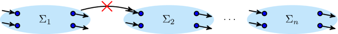
• Sequential. c is a sequence cut in $\alpha _{\text {dfg}}$ if $\oplus = \rightarrow$ and

s.1:

Each node in a part is indirectly and only connected to all nodes in the parts “after” it:

$\forall _{1 \leqslant i < j \leqslant n}~ \forall _{a \in \Sigma _i, b \in \Sigma _j}~ \alpha _{\text {dfg}}\!\!^{+}\!(a, b) \wedge \lnot \alpha _{\text {dfg}}\!\!^{+}\!(b, a)$:

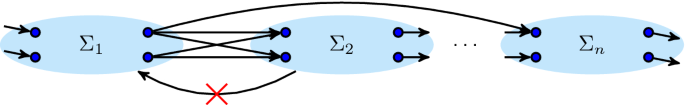
• Interleaved. c is an interleaved cut in $\alpha _{\text {dfg}}$ if $\oplus = \leftrightarrow$ and

i.1:

Between parts, all and only connections exist from an end to a start activity:

$\forall _{1 \leqslant i \leqslant n, 1 \leqslant j \leqslant n, i \ne j}~ \forall _{a \in \Sigma _i, b \in \Sigma _j}~ \alpha _{\text {dfg}}(a, b) \Leftrightarrow (a \in {{\,\mathrm{End}\,}}\wedge b \in {{\,\mathrm{Start}\,}})$):

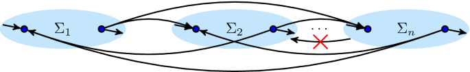
• Concurrent. c is a concurrent cut in $\alpha _{\text {dfg}}$ if $\oplus = \wedge$ and

c.1:

Each part contains a start and an end activity:

$\forall _{1 \leqslant i \leqslant n}~ {{\,\mathrm{Start}\,}}(\alpha _{\text {dfg}}) \cap \Sigma _i \ne \emptyset \wedge {{\,\mathrm{End}\,}}(\alpha _{\text {dfg}}) \cap \Sigma _i \ne \emptyset$

c.2:

All parts are fully interconnected:

$\forall _{1 \leqslant i < n, 1 \leqslant j \leqslant n, i \ne j}~ \forall _{a \in \Sigma _i, b \in \Sigma _j}~ \alpha _{\text {dfg}}(a, b) \wedge \alpha _{\text {dfg}}(b, a)$):

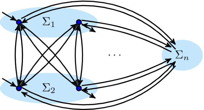
• Loop. c is a loop cut in $\alpha _{\text {dfg}}$ if $\oplus \,=\,\circlearrowleft$ and

l.1:

All start and end activities are in the body (i.e. the first) part:

${{\,\mathrm{Start}\,}}(\alpha _{\text {dfg}}) \cup {{\,\mathrm{End}\,}}(\alpha _{\text {dfg}}) \subseteq \Sigma _1$

l.2:

Only start/end activities in the body part have connections from/to other parts:

$\forall _{2 \leqslant j \leqslant n}~ \forall _{a \in \Sigma _1, b \in \Sigma _j}~ \alpha _{\text {dfg}}(a, b) \Rightarrow a \in {{\,\mathrm{End}\,}}(\alpha _{\text {dfg}})$

$\forall _{2 \leqslant j \leqslant n}~ \forall _{a \in \Sigma _1, b \in \Sigma _j}~ \alpha _{\text {dfg}}(b, a) \Rightarrow a \in {{\,\mathrm{Start}\,}}(\alpha _{\text {dfg}})$

l.3:

Redo parts have no connections to other redo parts:

$\forall _{2 \leqslant i \leqslant n, 2 \leqslant j \leqslant n, i\ne j}~ \forall _{a \in \Sigma _i, b \in \Sigma _j}~ \lnot \alpha _{\text {dfg}}(a, b) \wedge \lnot \alpha _{\text {dfg}}(b, a)$

l.4:

If an activity from a redo part has a connection to/from the body part, then it has connections to/from all start/end activities:

$\forall _{2 \leqslant i \leqslant n}~ \forall _{a \in {{\,\mathrm{Start}\,}}, b \in \Sigma _i}~ \alpha _{\text {dfg}}(b, a) \Leftrightarrow \forall _{c \in {{\,\mathrm{Start}\,}}(\alpha _{\text {dfg}})}~ \alpha _{\text {dfg}}(b, c)$

$\forall _{2 \leqslant i \leqslant n}~ \forall _{a \in {{\,\mathrm{End}\,}}, b \in \Sigma _i}~ \alpha _{\text {dfg}}(a, b) \Leftrightarrow \forall _{c \in {{\,\mathrm{End}\,}}(\alpha _{\text {dfg}})}~ \alpha _{\text {dfg}}(c, b)$):

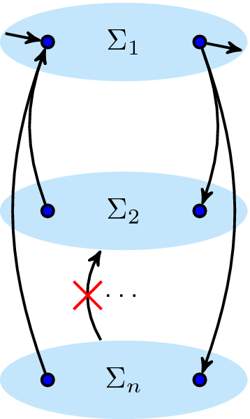
1.2 Minimum self-distance (Definition 6.3)

Let $\alpha _{\text {msd}}$ be a minimum self-distance graph and let $c = (\oplus , \Sigma _1, \ldots \Sigma _n)$ be a cut, consisting of a process tree operator and a partition of activities with parts $\Sigma _1 \ldots \Sigma _n$ such that $\Sigma (\alpha _{\text {msd}}) = \bigcup _{1 \leqslant i \leqslant n} \Sigma _i$ and $\forall _{1 \leqslant i < j \leqslant n}~ \Sigma _i \cap \Sigma _j = \emptyset$.

• Concurrent and interleaved. If $\oplus = \wedge$ or $\oplus = \leftrightarrow$, then in $\alpha _{\text {msd}}$:

ci.1:

There are no $\alpha _{\text {msd}}$ connections between parts:

$\forall _{i \in [1\ldots n], i \ne j \in [1 \ldots n]}~ \forall _{a \in \Sigma _i, b \in \Sigma _j}~ \lnot \alpha _{\text {msd}}(a, b)$):

• Loop. If $\oplus = \circlearrowleft$ then in $\alpha _{\text {msd}}$:

l.1:

Each activity has an outgoing edge:

$\forall _{a \in \Sigma (\alpha _{\text {msd}})}~ \exists _{b \in \Sigma (\alpha _{\text {msd}}), b \ne a}~ \alpha _{\text {msd}}(a, b)$

l.2:

All redo activities that have a connection to a body activity have connections to the same body activities:

$$\begin{aligned} \forall _{2 \leqslant i \leqslant n, 2 \leqslant j \leqslant n}~ \forall _{a \in \Sigma _i, b \in \Sigma _j}~&(\{ c \mid {\alpha _{\text {msd}}(a, c)} \} \cap \Sigma _1 \ne \emptyset \wedge {}\\&\{c \mid {\alpha _{\text {msd}}(b, c)} \} \cap \Sigma _1 \ne \emptyset ) \Rightarrow {}\\&\{c \mid {\alpha _{\text {msd}}(a, c)}\} \cap \Sigma _1 = \{c \mid {\alpha _{\text {msd}}(b, c)}\} \cap \Sigma _1 \end{aligned}$$

l.3:

All body activities that have a connection to a redo activity have connections to the same redo activities:

$$\begin{aligned} \forall _{a, b \in \Sigma _1}~&(\{ c \mid {\alpha _{\text {msd}}(a, c)} \} \cap \Sigma (\alpha _{\text {msd}}) \setminus \Sigma _1 \ne \emptyset \wedge {}\\&\{ c \mid {\alpha _{\text {msd}}(b, c)} \} \cap \Sigma (\alpha _{\text {msd}}){\setminus }\Sigma _1 \ne \emptyset ) \Rightarrow {}\\&\{ c \mid {\alpha _{\text {msd}}(a, c)} \} \cap \Sigma (\alpha _{\text {msd}}){\setminus }\Sigma _1 = \{ c \mid {\alpha _{\text {msd}}(b, c)} \} \cap \Sigma (\alpha _{\text {msd}}){\setminus }\Sigma _1 \end{aligned}$$

l.4:

No two activities from different redo children have an $\alpha _{\text {msd}}$-connection:

$\forall _{2 \leqslant i < j \leqslant n}~ \forall _{a \in \Sigma _i, b \in \Sigma _j}~ \lnot \alpha _{\text {msd}}(a, b) \wedge \lnot \alpha _{\text {msd}}(b, a)$

1.3 Sequence with -constructs: (Definition 7.3)

Let $\Sigma$ be an alphabet of activities, let $\alpha _{\text {dfg}}$ be a directly follows graph over $\Sigma$ and let $C = (\rightarrow , S_1, \ldots S_m)$ be a $\rightarrow$-cut of $\alpha _{\text {dfg}}$ according to Definition 5.2. Then, a partial cut $(\rightarrow , \Sigma _1, \ldots \Sigma _n)$ is a partial $\rightarrow$-cut if there is a pivot$\Sigma _p$ such that:

s.1:

The partial cut is a consecutive part of C:

$\exists _{1 \leqslant s \leqslant m}~ \forall _{1 \leqslant j \leqslant n}~ S_{s + j - 1} = \Sigma _j$

s.2:

There are no end activities before the pivot in the partial cut:

$\forall _{x \in [1 \ldots p - 1]}~ \Sigma _x \cap {{\,\mathrm{End}\,}}(\alpha _{\text {dfg}}) = \emptyset$

s.3:

There are no start activities after the pivot in the partial cut:

$\forall _{x \in [p + 1 \ldots n]}~ \Sigma _x \cap {{\,\mathrm{Start}\,}}(\alpha _{\text {dfg}}) = \emptyset$

s.4:

There are no directly follows edges bypassing the pivot in the partial cut:

$\forall _{x \in [1 \ldots p - 1]}~ \forall _{a \in \Sigma _x}~ \forall _{\alpha _{\text {dfg}}(a, b)}~ \exists _{y \in [1 \ldots p]}~ b \in \Sigma _y$

$\forall _{y \in [p + 1 \ldots n]}~ \forall _{b \in \Sigma _y}~ \forall _{\alpha _{\text {dfg}}(a, b)}~ \exists _{x \in [p \ldots n]}~ a \in \Sigma _x$

s.5:

The partial cut can be tightly avoided:

$$\begin{aligned} \begin{aligned}&\exists _{1 \leqslant x< s, s + n \leqslant y \leqslant m}~ \exists _{a \in S_x, b \in S_y}~ \alpha _{\text {dfg}}(a, b) \\ {} \vee {}&\exists _{1 \leqslant x < s}~ \exists _{a \in S_x}~ a \in {{\,\mathrm{End}\,}}(\alpha _{\text {dfg}}) \\ {} \vee {}&\exists _{s + n \leqslant y \leqslant m}~ \exists _{b \in S_y}~ b \in {{\,\mathrm{Start}\,}}(\alpha _{\text {dfg}}) \\ {} \vee {}&\epsilon \in \alpha _{\text {dfg}}\end{aligned} \end{aligned}$$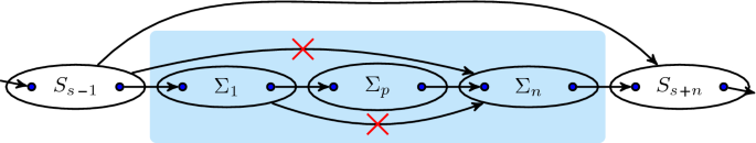

end of definition

Partial cuts are considered only when close enough to the root of the process tree. We formalize this in sequence-optional stems (${{\,\mathrm{so-stem}\,}}$s). If we consider a process tree as a graph, then the so-stem is the connected subgraph that starts at the root of the tree and that consists of $\rightarrow$- and -nodes. In addition, -nodes are only included if such nodes have two children of which one is a $\tau$:

Definition B.1

(sequence-optional tree and stem) A reduced process tree $M = \oplus (M_1,\ldots M_n)$ is a so-tree if and only if $\oplus = \rightarrow$, or if , $n = 2$ and $M_i = \tau$ for some $i\in [1\ldots n]$. The so-stem of a reduced process tree M is the smallest set ${{\,\mathrm{so-stem}\,}}(M)$ with:

• if M is a so-tree, then $M \in {{\,\mathrm{so-stem}\,}}(M)$;

• for each $\oplus (M_1,\ldots M_n) \in {{\,\mathrm{so-stem}\,}}(M)$ and each $M_i, i\in [1\ldots n]$ holds: if $M_i$ is a so-tree, then $M_i \in {{\,\mathrm{so-stem}\,}}(M)$

(For this set, we assume that subtrees can be distinguished.)

For instance, the following tree has an ${{\,\mathrm{so-stem}\,}}$, and $P_1$, $P_2$ and $P_4$ are non-optional non-sequential subtrees:

All subtrees shown here are sequential. Some subtrees can be skipped, however dependencies exist: if a subtree is executed, then each “P-sibling” at any higher level is executed as well. For instance, if $\ldots _3$ is executed, then $P_2$ is executed, as well as $P_1$. The challenge in preserving information in the abstraction is to not combine $P_1$ with $P_2$ in a partial cut without $\ldots _3$ and not to combine $\ldots _3$ and $P_4$ without $P_2$.

Lemma B.1

(Partial $\rightarrow$-cut for process trees) Let M be a reduced process tree without duplicate activities and with an ${{\,\mathrm{so-stem}\,}}$, and let . Let S be a partition of $\Sigma (M)$ such that $\forall _{i \in [1 \ldots n]}~ \Sigma (M'_i) \in S$ . Then, $(\rightarrow , \Sigma (M'_1), \ldots \Sigma (M'_n))$ is a partial $\rightarrow$-cut of $\alpha _{\text {dfg}}(M)$ over S.

By the reduction rules, at least one of the children is not optional: $\exists _{i \in [1 \ldots n]}~ \lnot {\overline{?}}(M_i)$. This child is the pivot. By the reduction rules, a pivot cannot be a sequential node itself. Then, this lemma follows from inspection of semantics of process trees.

1.4 Concurrent-optional-Or: (Definition 7.7)

Let $\Sigma$ be an alphabet of activities, S a partition of $\Sigma$, let $\alpha _{\text {coo}}(S)$ be a coo-graph, let $\alpha _{\text {dfg}}$ be a directly follows graph, and let be a partial cut such that $\forall _{1 \leqslant i \leqslant n}~ \Sigma _i \in S$. Then, C is a partial -cut if in $\alpha _{\text {coo}}(S)$ and $\alpha _{\text {dfg}}$:

o.1:

C is a part of a concurrent cut $(\wedge , X_1, \ldots X_m)$ (Definition 5.2):

$\forall _{1 \leqslant i \leqslant n}~ \exists _{1 \leqslant j \leqslant m}~ \Sigma _i = X_j$

o.2:

all parts are interchangeable in $\alpha _{\text {coo}}(S)$:

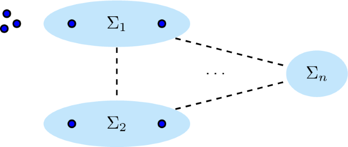
1.5 Concurrent-optional-Or: $\wedge$ (Definition 7.8)

Let $\Sigma$ be an alphabet of activities, S a partition of $\Sigma$, let $\alpha _{\text {coo}}(S)$ be a coo-graph, let $\alpha _{\text {dfg}}$ be a directly follows graph, and let $C = (\wedge , \Sigma _1, \ldots \Sigma _n)$ be a partial cut such that $\forall _{1 \leqslant i \leqslant n}~ \Sigma _i \in S$. Then, C is a partial $\wedge$-cut if in $\alpha _{\text {coo}}(S)$ and $\alpha _{\text {dfg}}$:

c.1:

C is a part of a concurrent cut $(\wedge , X_1, \ldots X_m)$ (Definition 5.2):

$\forall _{1 \leqslant i \leqslant n}~ \exists _{1 \leqslant j \leqslant m}~ \Sigma _i = X_j$

• Furthermore, in $\alpha _{\text {coo}}(S)$:

• – EITHER –

c.2.1:

all parts bi-imply one another:

$\forall _{1 \leqslant i < j \leqslant n}~ \Sigma _i\,\overline{\Rightarrow }\,\Sigma _j \wedge \Sigma _j\,\overline{\Rightarrow }\, \Sigma _i$

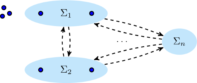
• – OR –

c.3.1:

the first part is optional:

${\overline{?}}{\Sigma _1}$

c.3.2:

The first part implies the other parts:

$\forall _{i \in [2\ldots n]}~ \Sigma _1\,\overline{\Rightarrow }\,\Sigma _i$

c.3.3:

All non-first parts bi-imply one another:

$\forall _{i, j \in [2\ldots n] \wedge i \ne j}~\Sigma _i\,\overline{\Rightarrow }\,\Sigma _j$

c.3.4:

No non-first part $\Sigma _i$ is implied by any part not in C:

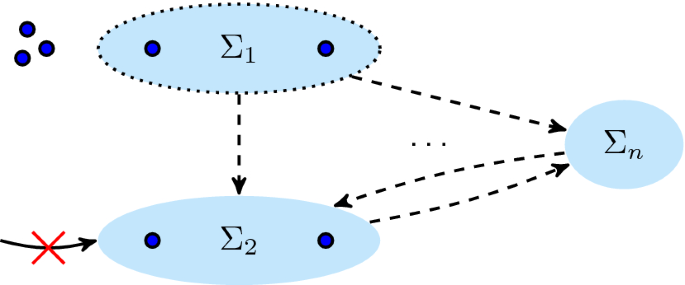
end of definition

Similar to so-stems, when considering a process tree M as a graph, the coo-stem of M is the connected subgraph starting at the root of M consisting of $\wedge$-, -, and nodes (the latter ones only if they have two children of which one is a $\tau$).

Definition B.2

(concurrent-optional-or tree and stem) A reduced process tree $M = \oplus (M_1,\ldots M_n)$ is a coo-tree if and only if , or if , $n = 2$ and $M_i = \tau$ for some $i\in [1\ldots n]$. The coo-stem of a reduced process tree M is the smallest set ${{\,\mathrm{coo-stem}\,}}(M)$ with:

• if M is a coo-tree, then $M \in {{\,\mathrm{coo-stem}\,}}(M)$;

• for each $\oplus (M_1,\ldots M_n) \in {{\,\mathrm{coo-stem}\,}}(M)$ and each $M_i, i\in [1\ldots n]$ holds: if $M_i$ is a coo-tree, then $M_i \in {{\,\mathrm{coo-stem}\,}}(M)$

(For this set, we assume that subtrees can be distinguished.)

Lemma B.2

(partial $\wedge$- and -cuts for process trees) Let M be a reduced process tree without duplicate activities and with an ${{\,\mathrm{coo-stem}\,}}$, and let $M' = \oplus (M'_1, \ldots M'_n) \in {{\,\mathrm{coo-stem}\,}}$, with . Let S be a partition of $\Sigma (M)$ such that $\forall _{i \in [1\ldots n]}~\Sigma (M'_i) \in S$. Then, $(\oplus , \Sigma (M'_1), \ldots \Sigma (M'_n))$ is a partial $\oplus$-cut of the coo-graph $\alpha _{\text {coo}}(\mathcal {L}(M), S)$.

This lemma follows from inspection of the semantics of process trees.

Class counterexamples

1.1 $\textsc {C}_{\text {dfg}}$

See Figs. 14, 15 and 16.

Fig. 14

An example for the necessity of Requirement $\hbox {C}_{\mathrm{dfg}}.\hbox {i}.1$: the trees have different languages but equivalent directly follows graphs. These trees differ in their root operator: activity e can be executed before and after all other activities, making the difference between interleaved and concurrent invisible

Fig. 15

An example for the necessity of Requirement $\hbox {C}_{\mathrm{dfg}}.\hbox {i}.2$: four trees having different languages but equivalent directly follows graphs. The difference between these trees is “semi-long-dependencies”, e.g.  in $M_{23}$, a cannot be executed between b and c, and such dependencies cannot be captured by a directly follows relation

Fig. 16

An example for the necessity of Requirement $\hbox {C}_{\mathrm{dfg}}.\hbox {i}.3$. Activity e witnesses ambiguity: e can be concurrent to ($M_{27}$) or interleaved to all other activities ($M_{28}$)

Uniqueness for $\alpha _{\text {dfg}}$

1.1 Lemma 5.2

Lemma: Take two reduced process trees of $\textsc {C}_{\text {dfg}}$$K = \oplus (K_1, \ldots K_n)$ and $M = \otimes (M_1, \ldots M_m)$ such that $\oplus \ne \otimes$. Then, $\alpha _{\text {dfg}}(K) \ne \alpha _{\text {dfg}}(M)$.

Proof

Towards contradiction, assume that $\alpha _{\text {dfg}}(K) = \alpha _{\text {dfg}}(M)$. By the reduction rules of Sect. 4, $n \geqslant 2$ and $m \geqslant 2$. Perform case distinction on $\oplus$ to prove that $\alpha _{\text {dfg}}(K) \ne \alpha _{\text {dfg}}(M)$.

• By semantics of the operator and the reduction rules, there exist at least n unconnected parts in $\alpha _{\text {dfg}}(K)$ (see Lemma 5.1). As and by the semantics of the other operators, $\alpha _{\text {dfg}}(M)$ is connected, so $\alpha _{\text {dfg}}(K) \ne \alpha _{\text {dfg}}(M)$.

• $\oplus = \rightarrow$ By semantics of the $\rightarrow$ operator, $\alpha _{\text {dfg}}(K)$ is a chain of at least n clusters (see Lemma 5.1). As $\otimes \ne \rightarrow$ and by the semantics of the other operators, $\alpha _{\text {dfg}}(M)$ is not a chain (for , the graph is not connected while for $\leftrightarrow$, $\wedge$ and $\circlearrowleft$, the graph is a clique), so $\alpha _{\text {dfg}}(K) \ne \alpha _{\text {dfg}}(M)$.

• $\oplus = \wedge$ By semantics of the $\wedge$ operator, $\alpha _{\text {dfg}}(K)$ consists of at least n fully interconnected clusters (see Lemma 5.1). Perform case distinction on the (due to symmetry) remaining cases of $\otimes$:

  • $\otimes \,=\,\circlearrowleft$ We try to construct a concurrent cut $(\wedge , \Sigma _1, \ldots \Sigma _p)$ for M. Take an activity $a \in {{\,\mathrm{Start}\,}}(M_1)$. By Requirement $\hbox {C}_{\mathrm{dfg}}.\hbox {l}.1$, $a \notin {{\,\mathrm{End}\,}}(M_1)$. Take an activity $b \in \Sigma (M) \setminus \Sigma (M_1)$. Then, by semantics of $\circlearrowleft$, $\lnot \alpha _{\text {dfg}}(a, b)$ and by Requirement c.2, a and b are part of the same $\Sigma$ in the cut we are constructing, e.g.  $\Sigma _1$. This holds for all a and b, thus $\Sigma (M) = \Sigma _1$. Hence, there is no non-trivial concurrent cut, and $\alpha _{\text {dfg}}(K) \ne \alpha _{\text {dfg}}(M)$.

  • $\otimes \,=\, \leftrightarrow$ By $\textsc {C}_{\text {dfg}}$, $\exists _{1\leqslant i \leqslant n}~ \exists _{a \in \Sigma (M_i)}~ a \notin {{\,\mathrm{Start}\,}}(M_i) \vee a \notin {{\,\mathrm{End}\,}}(M_i)$. Take such an $M_i$ and a. As either $a \notin {{\,\mathrm{Start}\,}}(M_i)$ or $a \notin {{\,\mathrm{End}\,}}(M_i)$, there is no connection to/from a to any other subtree, i.e. $\forall _{1 \leqslant j \leqslant n, j \ne i}~ \forall _{b \in \Sigma (M_j)}~ \lnot \alpha _{\text {dfg}}(b, a) \vee \lnot \alpha _{\text {dfg}}(a, b)$. If we would construct a concurrent cut $(\wedge , \Sigma _1 \ldots \Sigma _p)$, then both a and all such b’s would be in the same $\Sigma$, e.g.  $\{a\} \cup (\Sigma (K) \setminus \Sigma (M_j)\}) \subseteq \Sigma _1$. This holds for all activities of ${{\,\mathrm{Start}\,}}(M_i)$ and ${{\,\mathrm{End}\,}}(M_i)$. Hence, if we would construct a concurrent cut, all ${{\,\mathrm{Start}\,}}(K)$ and ${{\,\mathrm{End}\,}}(K)$ activities would be part of the same $\Sigma$. Therefore, there cannot be a non-trivial concurrent cut for K, and hence, $\alpha _{\text {dfg}}(K) \ne \alpha _{\text {dfg}}(M)$.

• $\oplus \,=\, \circlearrowleft$ Perform case distinction on the remaining case of $\otimes$:

  • $\otimes \,=\, \leftrightarrow$ We try to construct a loop cut $(\circlearrowleft , \Sigma _1, \ldots \Sigma _n)$. Consider a child $M_i$, and an activity s from the start activities of another child. Moreover, consider a path $\alpha _{\text {dfg}}(a_1, a_2) \ldots \alpha _{\text {dfg}}(a_{p-1}, a_p)$ such that all activities on the path are in $\Sigma (M_i)$, and $a_1 \in {{\,\mathrm{Start}\,}}(M_i)$ and $a_p \in {{\,\mathrm{End}\,}}(M_i)$. By Lemma 5.1, $a_1 \in \Sigma _1 \wedge a_p \in \Sigma _1$. Consider activity $a_2$. If $a_2 \in {{\,\mathrm{Start}\,}}(M_i)$, then $a_2 \in \Sigma _1$. If $a_2 \in {{\,\mathrm{End}\,}}(M_i)$, then $a_2 \in \Sigma _1$. If $a_2 \notin {{\,\mathrm{Start}\,}}(M_i) \wedge a_2 \notin {{\,\mathrm{End}\,}}(M_i)$, then by the semantics of $\leftrightarrow$, $\lnot \alpha _{\text {dfg}}(s, a_2)$. If $a_2$ would be in $\Sigma _2$, as it has a connection $\alpha _{\text {dfg}}(a_1, a_2)$, by the semantics of $\circlearrowleft$ there should be a connection $\alpha _{\text {dfg}}(s, a_2)$. Thus, $a_2 \in \Sigma _1$. This argument holds for the entire path, and by construction of $\alpha _{\text {dfg}}(M)$ each activity is on such a path; thus, $\Sigma (M_i) \subseteq \Sigma _1$. This holds for all children $M_i$, so there cannot be a non-trivial loop cut. Hence, $\alpha _{\text {dfg}}(K) \ne \alpha _{\text {dfg}}(M)$.

As these arguments are symmetric in $\oplus$ and $\otimes$, we conclude that $\alpha _{\text {dfg}}(K) \ne \alpha _{\text {dfg}}(M)$. $\square$

1.2 Lemma 5.3

Lemma: Take two reduced process trees of $\textsc {C}_{\text {dfg}}$$K = \oplus (K_1 \ldots K_n)$ and $M = \oplus (M_1 \ldots M_m)$ such that their activity partition is different: $\exists _{1 \leqslant w \leqslant \text {min}(n, m)}~ \Sigma (K_w) \ne \Sigma (M_w)$. Then, $\alpha _{\text {dfg}}(K) \ne \alpha _{\text {dfg}}(M)$.

Proof

Without loss of generality, we assume that children of the non-commutative operators ($\rightarrow$, $\circlearrowleft$) have a fixed order. Towards contradiction, assume that $\alpha _{\text {dfg}}(K) = \alpha _{\text {dfg}}(M)$. Perform case distinction on $\oplus$ (the case for K and M swapped is symmetric):

• Take a pair of activities a, b such that $a \in \Sigma (K_x)$, $a \in \Sigma (M_y)$, $b \in \Sigma (K_x)$ and $b \notin \Sigma (M_y)$ (choose x and y as desired). Obviously, if the activity partitions of K and M are different such a pair exists. By the reduction rules, no child $K_1 \ldots K_n$ is an exclusive-choice subtree itself, and by semantics of the other operators there is an undirected path in $\alpha _{\text {dfg}}(K)$, i.e. $a \leftrightsquigarrow b$ in $\alpha _{\text {dfg}}(K)$. However, as $a \in \Sigma (M_y) \wedge b \notin \Sigma (M_y)$, in $\alpha _{\text {dfg}}(M)$. Hence, $\alpha _{\text {dfg}}(K) \ne \alpha _{\text {dfg}}(M)$.

• $\oplus = \rightarrow$ Take $a \in \Sigma (K_i)$ and $b \in \Sigma (K_j)$ such that $i < j$. Then by the $\rightarrow$-cut, $\alpha _{\text {dfg}}\!\!^{+}\!(a, b) \wedge \lnot \alpha _{\text {dfg}}\!\!^{+}\!(b, a)$. By the reduction rules, all children of K and M are not $\rightarrow$-nodes themselves, thus, by the semantics of the other operators ( is unconnected, $\wedge$ and $\circlearrowleft$ are strongly connected), either $\lnot \alpha _{\text {dfg}}(a, b)$ or $\alpha _{\text {dfg}}\!\!^{+}\!(b, a)$. Then, $a \in \Sigma (M_x) \wedge b \in \Sigma (M_y)$ with $x < y$. This holds for all such a and b, hence $\forall _{1 \leqslant i \leqslant n = m}~ \Sigma (K_i) = \Sigma (M_i)$, which contradicts the initial assumption.

• $\oplus = \wedge$ To prove the equality of the activity partitions, we consider two symmetrical directions: a) if two activities are in the same $\Sigma _i$ in K, then they are in the same $\Sigma _i$ in M. b) if two activities are in the same $\Sigma _i$ in M, then they are in the same $\Sigma _i$ in K.

  Consider a child $M_x$. Perform case distinction on the structure of $M_x$:

  • $M_x = a$ A single activity cannot be split. Thus, $\Sigma (K_x) \subseteq \Sigma (M_x)$.

  • Take two activities $a \in \Sigma (M_{x_1})$ and $b \in \Sigma (M_{x_2})$. By semantics of , $\lnot \alpha _{\text {dfg}}(a, b)$. Thus, in a concurrent cut, a and b should be part of the same $\Sigma$. This holds for all such activities of all children of $M_x$; thus, $\Sigma (K_x) \subseteq \Sigma (M_x)$.

  • $M_x \,=\,\rightarrow (M_{x_1}, \ldots M_{x_p})$ Similar, using that either $\lnot \alpha _{\text {dfg}}(a, b)$ or $\lnot \alpha _{\text {dfg}}(b, a)$.

  • $M_x \,=\, \wedge (M_{x_1}, \ldots M_{x_p})$ Excluded by the reduction rules.

  • $M_x \,=\, \circlearrowleft (M_{x_1}, \ldots M_{x_p})$ By $\textsc {C}_{\text {dfg}}$, there is at least one child $M_{x_i}$ such that ${{\,\mathrm{Start}\,}}(M_{x_i})$${}\cap {}$${{\,\mathrm{End}\,}}(M_{x_i}) = \emptyset$. Take such a $M_{x_i}$ and an a from $\Sigma (M_{x_i})$. Furthermore, take b from any other child. There are three cases for a: $a \notin {{\,\mathrm{Start}\,}}(M_{x_i})$, $a \notin {{\,\mathrm{End}\,}}(M_{x_i})$ or both. For all these three cases, $\lnot \alpha _{\text {dfg}}(a, b) \vee \lnot \alpha _{\text {dfg}}(b, a)$. Thus, by argumentation similar to the case, $\Sigma (K_x) \subseteq \Sigma (M_x)$.

  • $M_x \,=\, \leftrightarrow (M_{x_1}, \ldots M_{x_p})$ Similar to the $\circlearrowleft$ case.

  Hence, $\Sigma (K_x) \subseteq \Sigma (M_x)$. This holds for all $\Sigma (M_x)$ and by symmetry for all $\Sigma (K_x)$. Hence, $\forall _{1 \leqslant i \leqslant n}~ \Sigma (K_i) = \Sigma (M_i)$, which contradicts the initial assumption.

  • $\oplus \,=\, \circlearrowleft$ Consider $\Sigma (K_i)$ for some $2 \leqslant i \leqslant n$. By the reduction rules, $K_i$ is of the form . By semantics of the other operators, for all $a, b \in \Sigma (K_i)$, there exists an undirected path $a \leftrightsquigarrow b$ in $\alpha _{\text {dfg}}(K)$, such that all activities on this undirected path are in $K_i$. Between all the activities on this path, there exists a connection in $\alpha _{\text {dfg}}(K_i)$, and none of the activities on this path is in ${{\,\mathrm{Start}\,}}(K)$ or ${{\,\mathrm{End}\,}}(K)$. By Lemma 5.1, in a non-trivial loop cut, (without loss of generality) $\Sigma (K_i) \subseteq \Sigma (M_i)$.

    Let $K_1 \,=\, \otimes (K_{1_1}, \ldots K_{1_p})$. Perform case distinction on $\otimes$:

  • Take a child $K_{1_i}$. By the reduction rules, this child is not an . For all activities $a \in {{\,\mathrm{Start}\,}}(K_{1_i}), b \in {{\,\mathrm{End}\,}}(K_{1_i})$, there exist a directed path $\alpha _{\text {dfg}}\!\!^{+}\!(a, b)$, such that this path is completely in $\Sigma (K_{1_i})$. Furthermore, take an activity $c \in {{\,\mathrm{End}\,}}(K_{1_{j \ne i}})$. By semantics of , c has no directly follows connection to any node on the path. Towards contradiction, assume there is a first node d on the path $\notin \Sigma (M_1)$. Then, by semantics of $\circlearrowleft$, there should be a connection $\alpha _{\text {dfg}}(c, d)$. This holds for all activities d and children i, so $\Sigma (K_1) \subseteq \Sigma (M_1)$.

  • $\otimes \,=\, \rightarrow$ Similar to the -case.

  • $\otimes \,=\, \wedge$${{\,\mathrm{Start}\,}}(K) \cup {{\,\mathrm{End}\,}}(K) \subseteq \Sigma (M_1)$, thus we only need to consider non-start non-end activities. Take such an activity a in child $K_{1_i}$, and take an activity $b \in {{\,\mathrm{End}\,}}(K_{1_{j \ne i}})$. By semantics of $\wedge$, $\alpha _{\text {dfg}}(a, b)$; by $\textsc {C}_{\text {dfg}}$, $b \notin {{\,\mathrm{Start}\,}}(K_1)$; thus by Lemma 5.1, $a \in \Sigma (M_1)$. This holds for all a, so $\Sigma (K_1) \subseteq \Sigma (M_1)$.

  • $\otimes \,=\, \circlearrowleft$ Excluded by the reduction rules.

  • $\otimes \,=\, \leftrightarrow$ Similar to the -case.

• $\oplus \,=\, \leftrightarrow$ Take a w such that $\Sigma (K_w) \ne \Sigma (M_w)$ and let $K_w = \otimes (K_{w_1}\ldots K_{w_p})$. Perform case distinction on $\otimes$:

  • By semantics of , no end activity of $K_{w_1}$ has a connection to any start activity of any other $K_{w_j}$. Thus, as M contains an interleaved activity partition, $\Sigma (K_w) \subseteq \Sigma (M_w)$.

  • $\otimes \,=\, \rightarrow$ Similar to the case.

  • $\otimes \,=\, \wedge$ By $\textsc {C}_{\text {dfg}}$, at least one child of $K_w$ has disjoint start and end activities. Take such a child $K_{w_y}$, and consider two activities: $a \notin {{\,\mathrm{Start}\,}}(K_{w_y})$ and $b \in \Sigma (K_w) \setminus K_{w_y}$. By semantics of $\wedge$, $\alpha _{\text {dfg}}(b, a)$. Then, by Lemma 5.1, $a \in \Sigma (M_w)$ and $b \in \Sigma (M_w)$. This holds for all b and by symmetry for ${{\,\mathrm{Start}\,}}(K_{w_y}) \cup {{\,\mathrm{End}\,}}(K_{w_y})$. By semantics of $\leftrightarrow$, non-start non-end activities only have connections with start/end activities of $K_w$. Therefore, $\Sigma (K_w) \setminus ({{\,\mathrm{Start}\,}}(K_w) \cup {{\,\mathrm{End}\,}}(K_w)) \subseteq \Sigma (M_w)$. Hence, $\Sigma (K_w) \subseteq \Sigma (M_w)$.

  • $\otimes \,=\, \circlearrowleft$ By semantics of $\leftrightarrow$, non-start non-end activities only have connections with start/end activities of $K_w$. Therefore, $\Sigma (K_w) \setminus ({{\,\mathrm{Start}\,}}(K_w) \cup {{\,\mathrm{End}\,}}(K_w)) \subseteq \Sigma (M_w)$. All activities $\in {{\,\mathrm{Start}\,}}(K_w) \cup {{\,\mathrm{End}\,}}(K_w)$ have connections from/to ${{\,\mathrm{End}\,}}(K_{w_2}) \cup {{\,\mathrm{Start}\,}}(K_{w_2})$, thus ${{\,\mathrm{Start}\,}}(K_w) \cup {{\,\mathrm{End}\,}}(K_w) \subseteq \Sigma (M_w)$. Hence, $\Sigma (K_w) \subseteq \Sigma (M_w)$.

  • $\otimes \,=\, \leftrightarrow$ Excluded by $\textsc {C}_{\text {dfg}}$.

By contradiction, we conclude $\alpha _{\text {dfg}}{K} \ne \alpha _{\text {dfg}}{M}$. $\square$

Uniqueness for $\textsc {C}_{\text {msd}}$

Lemma E.1

(Operators are mutually exclusive) Take two reduced process trees of $\textsc {C}_{\text {msd}}$$K = \oplus (K_1, \ldots K_n)$ and $M = \otimes (M_1, \ldots M_m)$ such that $\oplus \ne \otimes$. Then, $\alpha _{\text {dfg}}(K) \ne \alpha _{\text {dfg}}(M)$ or $\alpha _{\text {msd}}(K) \ne \alpha _{\text {msd}}(M)$.

This proof of this lemma is similar to the proof of Lemma 5.2: for each combination of $\oplus$ and $\otimes$, a difference in $\alpha _{\text {msd}}$-graphs is shown. For a detailed proof, please refer to “Appendix E.2”.

Lemma E.2

(Partitions are mutually exclusive) Take two reduced process trees of $\textsc {C}_{\text {dfg}}$$K = \oplus (K_1 \ldots K_n)$ and $M = \oplus (M_1 \ldots M_m)$ such that their activity partition is different: $\exists _{1 \leqslant w \leqslant \text {min}(n, m)}~ \Sigma (K_w) \ne \Sigma (M_w)$. Then, $\alpha _{\text {dfg}}(K) \ne \alpha _{\text {dfg}}(M)$ or $\alpha _{\text {msd}}(K) \ne \alpha _{\text {msd}}(M)$.

This proof of this lemma is similar to the proof of Lemma 5.3: for each $\oplus$, it is shown that a difference in partitions must lead to a difference in $\alpha _{\text {msd}}$-graphs. For a detailed proof, please refer to “Appendix E.3”.

Lemma E.3

(Abstraction uniqueness for $\textsc {C}_{\text {msd}}$) Take two reduced process trees of class $\textsc {C}_{\text {msd}}$: $K = \oplus (K_1, \ldots K_n)$ and $M = \otimes (M_1, \ldots M_m)$. Then, $K = M$ if and only if $\alpha _{\text {dfg}}(K) = \alpha _{\text {dfg}}(M)$ and $\alpha _{\text {msd}}(K) = \alpha _{\text {msd}}(M)$.

The proof of this lemma is similar to the proof of Lemma 5.4, using Lemmas E.1 and E.2.

Corollary E.1

(Language uniqueness for $\textsc {C}_{\text {msd}}$) There are no two different reduced process trees of $\textsc {C}_{\text {msd}}$ with equal languages. Hence, for trees of class $\textsc {C}_{\text {msd}}$, the normal form of Sect. 4 is uniquely defined.

1.1 LC-property

The minimum self-distance graph possesses more expressive power than the footprints of Definition 6.3 utilize. That is, there exist pairs of process trees that have different normal forms, languages and $\alpha _{\text {msd}}$-graphs, but that the footprints do not distinguish.

For instance, consider the trees

and

These trees have a different language, an equivalent $\alpha _{\text {dfg}}$-graph (shown in Fig. 9b) but a different $\alpha _{\text {msd}}$-graph (shown in Fig. 9c, d). Thus, they could be distinguished using their $\alpha _{\text {msd}}$-graph.

However, the footprint (Definition 6.3) cannot distinguish these trees: both cuts $(\circlearrowleft , \{a, b, c\}, \{d\})$ and $(\circlearrowleft , \{a, c, d\}, \{b\})$ are valid in both $\alpha _{\text {msd}}$-graphs, where $(\circlearrowleft , \{a, b, c\}, \{d\})$ corresponds to $M_{12}$ and $(\circlearrowleft , \{a, c, d\}, \{b\})$ corresponds to $M_{13}$. This implies that a discovery algorithm that uses only the footprint cannot distinguish these two trees.

This problem occurs in certain nestings of loops and concurrent operators, as indicated in the proof of Lemma E.2. We formalize this remaining problem as a loop-concurrency property (LC-property). An LC-property could distinguish the specific nesting using only the $\alpha _{\text {msd}}$-graph.

Definition E.1

(LC-property) Let $K, M \in \textsc {C}_{\text {msd}}{}$ be process trees in normal form such that

and $\alpha _{\text {dfg}}(K) = \alpha _{\text {dfg}}(M)$. Then, an LC-propertyLC is a function that distinguishes the cuts of K and M in their minimum self-distance graphs, i.e. $LC(\alpha _{\text {msd}}(K)) \wedge LC(\alpha _{\text {msd}}(M))$ if and only if the cut $(\circlearrowleft , \Sigma (K_1), \ldots \Sigma (K_n))$ conforms to both K and M.

Consider $\textsc {C}_{\text {msd}}{}'$ to be the class of trees $\textsc {C}_{\text {msd}}{}$ where arbitrary nestings of $\circlearrowleft$ and $\wedge$ are allowed, that is, Requirement $\hbox {C}_{\mathrm{msd}}.\hbox {l}.1$ is dropped. Then, if an LC-property exists, Lemma E.2 applies for $\textsc {C}_{\text {msd}}{}'$.

We did not find an LC-property, but we also did not prove that it cannot exist. A proof that an LC-property cannot exist would, for instance, be the existence of an example of two process trees of $\textsc {C}_{\text {msd}}{}'$ in normal form with equivalent $\alpha _{\text {msd}}$-graphs. We did not find such examples in an extensive search, so we conjecture that an LC-property exists:

Conjecture E.1

(LC-property) There exists an LC-property (Definition E.1).

1.2 Lemma E.1

Lemma: Take two reduced process trees of $\textsc {C}_{\text {msd}}$$K = \oplus (K_1, \ldots K_n)$ and $M = \otimes (M_1, \ldots M_m)$ such that $\oplus \ne \otimes$. Then, $\alpha _{\text {dfg}}(K) \ne \alpha _{\text {dfg}}(M)$ or $\alpha _{\text {msd}}(K) \ne \alpha _{\text {msd}}(M)$.

Proof

Towards contradiction, assume $\alpha _{\text {dfg}}(K) = \alpha _{\text {dfg}}(M)$ and $\alpha _{\text {msd}}(K) = \alpha _{\text {msd}}(M)$. We only consider the cases that were not covered in the proof of Lemma 5.2.

• $\oplus = \wedge$ and $\otimes = \circlearrowleft$. We try to construct a concurrent cut $\Sigma _1 \ldots \Sigma _q$ for M. By Requirement c.1, every such $\Sigma _i$ must have a start and an end activity. Thus, we only need to prove that ${{\,\mathrm{Start}\,}}(M_1) \cup {{\,\mathrm{End}\,}}(M_1) \subseteq \Sigma _1$. Perform case distinction on $M_1$:

  • Each $a \in \Sigma (M_{1_i})$ has no $\alpha _{\text {dfg}}$-connection to any activity in $\Sigma (M_{j \ne i})$. Therefore, ${{\,\mathrm{Start}\,}}(M_1) \cup {{\,\mathrm{End}\,}}(M_1) \subseteq \Sigma _1$.

  • $M_1\,=\,\rightarrow (M_{1_1}, \ldots M_{1_p})$ Each $a \in \Sigma (M_{1_i})$ has no $\alpha _{\text {dfg}}$-connection to any activity in $\Sigma (M_{j < i})$. Therefore, ${{\,\mathrm{Start}\,}}(M_1) \cup {{\,\mathrm{End}\,}}(M_1) \subseteq \Sigma _1$.

  • $M_1 = \wedge (\ldots )$ Consider three cases:

    • If any of the $M_{2 \leqslant i \leqslant p}$ contains a $\circlearrowleft$, consider an activity a in the redo of that $\circlearrowleft$. By semantics of $\circlearrowleft$, there is no $\alpha _{\text {dfg}}$-connection between a and any activity in $\Sigma (M_1)$. Therefore, ${{\,\mathrm{Start}\,}}(M_1) \cup {{\,\mathrm{End}\,}}(M_1) \subseteq \Sigma _1$.

    • If none of the $M_{2 \leqslant i \leqslant p}$ contains a $\circlearrowleft$ and $M_1$ does not contain a $\circlearrowleft$, then the $\alpha _{\text {msd}}$-graph is connected, and therefore, by Requirement  ci.1, $\Sigma (M) \subseteq \Sigma _1$.

    • If none of the $M_{2 \leqslant i \leqslant p}$ contains a $\circlearrowleft$ and $M_1$ contains a $\circlearrowleft$, then consider an activity a under a redo of any such $\circlearrowleft$, and any activity $b \in \Sigma (M_{2 \leqslant i \leqslant m})$. By semantics of $\circlearrowleft$, $\lnot \alpha _{\text {dfg}}(a, b)$ and $\lnot \alpha _{\text {dfg}}(b, a)$, thus a and b must be in the same $\Sigma _1$. All activities ${{\,\mathrm{Start}\,}}(M_1) \cup {{\,\mathrm{End}\,}}(M_1)$ have at least an $\alpha _{\text {msd}}$-connection with at least some activity in the redo of a $\circlearrowleft$. Thus, by Requirement ci.1, ${{\,\mathrm{Start}\,}}(M_1) \cup {{\,\mathrm{End}\,}}(M_1) \subseteq \Sigma _1$.

  • $M_1\,=\,\circlearrowleft (\ldots )$ Excluded by $\textsc {C}_{\text {msd}}$.

  • $M_1\,=\, \leftrightarrow (\ldots )$ By $\textsc {C}_{\text {msd}}$, there exists a child $M_{1_i}$ such that ${{\,\mathrm{Start}\,}}(M_{1_i}) \cap {{\,\mathrm{End}\,}}(M_{1_i})\,=\,\emptyset$. Thus, all activities in ${{\,\mathrm{End}\,}}(M_{1_{j \ne i}})$ have no $\alpha _{\text {dfg}}$-connection to ${{\,\mathrm{End}\,}}(M_{1_i})$, and similarly for the activities of ${{\,\mathrm{Start}\,}}(M_{1_j})$. Therefore, ${{\,\mathrm{Start}\,}}(M_1) \cup {{\,\mathrm{End}\,}}(M_1) \subseteq \Sigma _1$.

  Hence, there is no concurrent cut in M, and therefore, $\alpha _{\text {dfg}}(K) \ne \alpha _{\text {dfg}}(M)$.

• $\oplus \,=\,\circlearrowleft$ and $\otimes \,=\,\leftrightarrow$. No change is necessary. $\square$

1.3 Lemma E.2

Lemma: Take two reduced process trees of $\textsc {C}_{\text {dfg}}$$K = \oplus (K_1 \ldots K_n)$ and $M = \oplus (M_1 \ldots M_m)$ such that their activity partition is different: $\exists _{1 \leqslant w \leqslant \text {min}(n, m)}~ \Sigma (K_w) \ne \Sigma (M_w)$. Then, $\alpha _{\text {dfg}}(K) \ne \alpha _{\text {dfg}}(M)$ or $\alpha _{\text {msd}}(K) \ne \alpha _{\text {msd}}(M)$.

Proof

Towards contradiction, assume that $\oplus = \otimes$, $\alpha _{\text {dfg}}(K) = \alpha _{\text {dfg}}(M)$, $\alpha _{\text {msd}}(K) = \alpha _{\text {msd}}(M)$ and that there is a w such that $\Sigma (K_w) \ne \Sigma (M_w)$. We only consider the cases that were not covered in the proof of Lemma 5.2.

• $\oplus = \wedge$ and $M_x\,=\,\circlearrowleft (M_{x_1},\ldots M_{x_p})$. Try to construct a $\wedge$-cut and prove that $\Sigma (M_x) \subseteq \Sigma _x$. Consider three cases:

  • If any of the $M_{x_{2 \leqslant i \leqslant p}}$ contains a $\circlearrowleft$, consider an activity a in the redo of that $\circlearrowleft$. By semantics of $\circlearrowleft$, there is no $\alpha _{\text {dfg}}$-connection between a and any activity in $\Sigma (M_{x_1})$. Therefore, $\Sigma (M_{x_1}) \subseteq \Sigma _x$. This holds for all such a, thus all such redo activities are in $\Sigma _x$. Consider all remaining activities, i.e. $b \in \Sigma (M_{x_{j \ne i}})$ such that b is in no other $\circlearrowleft$-redo than $M_x$. For each of these activities b, there is a $\alpha _{\text {msd}}$-relation with an activity in $\Sigma _{x_1}$ or an activity such as a. Thus, $\Sigma (M_x) \subseteq \Sigma _x$.

  • If none of the $M_{x_{2 \leqslant i \leqslant p}}$ contains a $\circlearrowleft$ and $M_{x_1}$ does not contain a $\circlearrowleft$, then the $\alpha _{\text {msd}}$-graph is connected, and therefore, $\Sigma (M_x) \subseteq \Sigma _x$.

  • If none of the $M_{x_{2 \leqslant i \leqslant p}}$ contains a $\circlearrowleft$ and $M_{x_1}$ contains a $\circlearrowleft$, then consider an activity a under a redo of any such $\circlearrowleft$, and any activity $b \in \Sigma (M_{x_{2 \leqslant i \leqslant m}})$. By semantics of $\circlearrowleft$, $\lnot \alpha _{\text {dfg}}(a, b)$ and $\lnot \alpha _{\text {dfg}}(b, a)$, thus a and b must be in the same $\Sigma _x$. All activities in $\Sigma (M_{x_1})$ have at least an $\alpha _{\text {msd}}$-connection with at least some activity in the redo of a $\circlearrowleft$, Thus, $\Sigma (M_x) \subseteq \Sigma _x$.

• $\oplus =\, \circlearrowleft$ and $K_1 = \wedge (K_{1, 1}, \ldots K_{1, p})$. Try to construct a $\circlearrowleft$-cut and prove that $\Sigma (K_1) \subseteq \Sigma _1$. By semantics of $\circlearrowleft$, ${{\,\mathrm{Start}\,}}(K_1) \cup {{\,\mathrm{End}\,}}(K_1) \subseteq \Sigma _1$. Take an activity $a \in \Sigma (K_1)$, such that $a \notin {{\,\mathrm{Start}\,}}(K_1) \cup {{\,\mathrm{End}\,}}(K_1)$, and take another $b \in \bigcup _{1 \leqslant i \leqslant n} \Sigma (K_i)$ such that $b \in {{\,\mathrm{Start}\,}}(K_1) \cup {{\,\mathrm{End}\,}}(K_1)$. Then, $b \in \Sigma _1$. Perform case distinction on b:

  • $b \notin {{\,\mathrm{End}\,}}(K_1)$ Then, $\alpha _{\text {dfg}}(b, a)$ and thus $a \in \Sigma _1$.

  • $b \notin {{\,\mathrm{Start}\,}}(K_1)$ Then, $\alpha _{\text {dfg}}(a, b)$ and thus $a \in \Sigma _1$.

  • $b \in {{\,\mathrm{Start}\,}}(K_1) \cap {{\,\mathrm{End}\,}}(K_1)$ Excluded by $\textsc {C}_{\text {msd}}$. (Here, the LC-property (Conjecture E.1) would detect and guarantee $a \in \Sigma _1$). $\square$

Uniqueness for $\alpha _{\text {coo}}$

Given a particular language, several partial cuts might apply. In this section, we prove that each of these partial cuts is “correct”, that is, corresponds to the process tree from which the language was derived. We first formalize this concept, after which we use it to prove uniqueness for so- and coo-stems.

Definition F.1

(partition correspondence, $\mathbb {M}^{\Sigma }$) Let M be a reduced process tree without duplicate activities. Then, $\mathbb {M}^{\Sigma }(M)$ denotes the set of all partitions S that correspond to M. That is, let $S = \{S_1, \ldots S_n\}$ be a partition of $\Sigma (M)$, then $S \in \mathbb {M}^{\Sigma }(M)$ if and only if there exists an $M'$ such that $M'$ reduces to M using only the associativity rules (, $\textsc {A}_{\rightarrow }{}$, $\textsc {A}_{\wedge }{}$, , $\textsc {A}_{\circlearrowleft \textsc {b}}{}$, $\textsc {A}_{\circlearrowleft \textsc {r}}{}$); and for every $S_i \in S$, there is a subtree $M''$ of $M'$ such that $S_i = \Sigma (M'')$.

Intuitively, a partition corresponds to a process tree if each set of activities in the partition can be mapped to a node in the process tree (up to the associativity rules). For instance, let

Then,

$$\begin{aligned} \mathbb {M}^{\Sigma }(M_{29}) = \{&\{ \{a\}, \{b\}, \{c\}, \{d\} \},&\{\{a, b\}, \{c\}, \{d\}\},&\{ \{a\}, \{b, c\}, \{d\} \}, \\&\{ \{a, c\}, \{b\}, \{d\} \},&\{ \{a, b, c\}, \{d\} \},&\{ \{a, b, c, d\} \} \}\\ \end{aligned}$$

Each of these partitions corresponds to $M_{29}$. For instance, consider the partition $\{\{a, c\}, \{b\}, \{d\}\}$. Each of the sets in this partition can be mapped on a node in the tree

which reduces to $M_{29}$ using the associativity rules. In this mapping, $\{d\}$ is mapped on the leaf d, $\{b\}$ is mapped on the leaf b, and $\{a, c\}$ is mapped on the node

In contrast, the partition $\{\{a, b\}, \{c, d\}\}$ does not correspond to $M_{29}$, as c and d cannot be mapped together without a and b.

1.1 SO-stems

In Lemma B.1, we showed that a tree with an structure has a partial $\rightarrow$-cut. Now, we prove the opposite: there can only be a partial $\rightarrow$-cut if the tree has such a structure.

Lemma F.1

(Partitions are mutually exclusive for so-stems) Let $M = \rightarrow (M_1, \ldots M_m)$, $K = \rightarrow (K_1, \ldots K_n)$ be reduced trees of $\textsc {C}_{\text {coo}}$ such that their activity partition is different, i.e. there is a $w \in [1 \ldots n]$ such that $\Sigma (K_w) \ne \Sigma (M_w)$. Then, $\alpha _{\text {dfg}}(M) \ne \alpha _{\text {dfg}}(K)$.

Proof

Towards contradiction, assume that $\alpha _{\text {dfg}}(K) = \alpha _{\text {dfg}}(M)$, and perform case distinction.

In case no child $K_i$ has the structure, $\alpha _{\text {dfg}}(K)$ is a chain of strongly connected or unconnected clusters, which correspond to $\Sigma (K_i)$’s. Notice that $\alpha _{\text {dfg}}$-edges can skip clusters, hence $\alpha _{\text {dfg}}(K)$ contains a maximal $\rightarrow$ cut. The same holds for $\alpha _{\text {dfg}}(M)$, and this holds for all such $\Sigma (K_i)$, so $\alpha _{\text {dfg}}(M) \ne \alpha _{\text {dfg}}(K)$.

In case at least one child $K_i$ has a structure , the corresponding cluster $\Sigma (K_i)$ is a chain itself. By Rule , at least one child of $K_i$ (say $K_{i_p}$) is a pivot (Definition 7.3). By Lemma B.1, $(\rightarrow , \Sigma (K_{i_1}), \Sigma (K_{i_k}) )$ is a partial $\rightarrow$-cut. Due to Requirement s.5, for every pivot, there is one partial $\rightarrow$-cut. The same holds for $\alpha _{\text {dfg}}(M)$, and this holds for all such $\Sigma (K_i)$, so $\alpha _{\text {dfg}}(M) \ne \alpha _{\text {dfg}}(K)$.

Hence, $\alpha _{\text {dfg}}(M) \ne \alpha _{\text {dfg}}(K)$. $\square$

1.2 Coo-stems

In Lemma B.2, we showed that a tree with a coo-stem has partial $\wedge$- and -cuts. In this section, we prove the opposite: there can only be a partial $\wedge$- and -cuts if the tree has such a corresponding coo-stem.

The main Lemmas, F.5 and F.6, consider partitions in a repetitive way: starting from a particular partition, a partial cut is considered, after which the sets of activities of the partial are merged in the partition, and a new, smaller, partition is obtained. For instance, the partition $\{\{a\}, \{b\}, \{c\}\}$ combined with the partial $\wedge$-cut $(\wedge , \{a\}, \{b\})$ becomes $\{\{a, b\}, \{c\}\}$. This reasoning procedure traverses the coo-stem of the process tree.

Invariant in the repetition is that every obtained partition corresponds to the process tree ($\mathbb {M}^{\Sigma }$). To keep the invariant, we prove that for any partition in $\mathbb {M}^{\Sigma }$, partial $\wedge$- and -cuts are always “correct” (Lemmas F.2 and F.3). Second, we prove that every obtained partition using such a partial cut is in $\mathbb {M}^{\Sigma }$ (Lemma F.4).

The repetition starts with the partition of the concurrent cut, which we formalize in Definition F.2. The repetition ends when the partial cut partitions the entire alphabet, and a contradiction is derived.

Definition F.2

(activity sets of non-coo-subtrees) Let M be a reduced process tree without duplicate activities. Then, ${\Sigma ^{\mathcal {C}}}(M)$ denotes the activity sets of the non-coo-subtrees of M:

Notice that ${\Sigma ^{\mathcal {C}}}(M)$ corresponds to a concurrent cut of the directly follows graph (Definition 5.2).

Lemma F.2

(partial -cut corresponds to ) Let $M \in \textsc {C}_{\text {coo}}{}$ be a reduced process tree with a coo-stem, let , $M' \in {{\,\mathrm{coo-stem}\,}}(M)$ be a coo-stem node, let $M'_i$ be a child of $M'$, let $S \in \mathbb {M}^{\Sigma }(M)$ be a partition such that $\Sigma (M'_i) \in S$, and let $\alpha _{\text {coo}}(S)$ be a coo-graph. Take any $A \in S$ such that $A \ne \Sigma (M'_i)$. Then, is a partial -cut of $\alpha _{\text {coo}}(S)$ if and only if $\exists _{1 \leqslant j \leqslant m}~ A = \Sigma (M'_j)$.

The proof of this lemma considers both directions of the bi-implication separately. Towards contradiction, it is assumed that such an A exists, after which semantics of sub-structures of M are used to derive a contradiction. “Appendix F.4” shows the detailed proof.

Lemma F.3

(partial $\wedge$-cut corresponds to $\wedge$) Let $M \in \textsc {C}_{\text {coo}}{}$ be a reduced process tree with a coo-stem, let $M' = \wedge (M'_1, \ldots M'_m)$, $M' \in {{\,\mathrm{coo-stem}\,}}(M)$ be a coo-stem node, let $M'_i$ be a child of $M'$, let $S \in \mathbb {M}^{\Sigma }(M)$ a partition such that $\Sigma (M'_i) \in S$, and let $\alpha _{\text {coo}}(\mathcal {L}(M), S)$ be a coo-graph. Take any $A \in S$ such that $A \ne \Sigma (M'_i)$. Then, $(\wedge , \Sigma (M'_i), A)$ or $(\wedge , A, \Sigma (M'_i))$ is a partial $\wedge$-cut of $\alpha _{\text {coo}}(\mathcal {L}(M), S)$ if and only if $\exists _{1 \leqslant j \leqslant m}~ A = \Sigma (M'_j)$.

The proof of this lemma is similar to the proof of Lemma F.2: the two directions are proven separately and semantics of sub-structures of M are used to derive a contradiction. For a detailed proof, see “Appendix F.5”.

Lemma F.4

(merge sigmaset preservation) Let M be a reduced process tree of $\textsc {C}_{\text {coo}}$ with a coo-stem. Let $S \in \mathbb {M}^{\Sigma }(M)$ and let $C = (\oplus , S_1, \ldots S_n)$ be a partial $\oplus$-cut of $\alpha _{\text {coo}}(\mathcal {L}(M), S)$. Let $S' = S \setminus \{S_1, \ldots S_n\} \cup \{\cup _{i \in [1 \ldots n]} S_i\}$ be S collapsed with respect to C. Then, $S' \in \mathbb {M}^{\Sigma }(M)$.

Proof

As $S \in \mathbb {M}^{\Sigma }(M)$, there must be a tree $M'$ to which S can be structurally mapped (Definition F.1). By Lemmas F.2 and F.3, for each $S_i$ there is a node $M'_i$ in $M'$ such that $S_i = \Sigma (M'_i)$. By the associativity rules, $M'$ can be transformed into $M''$ such that $M''$ contains a node $\oplus (M'_1, \ldots M'_n)$. Then, $S'$ can be structurally mapped to $M''$. Hence, $S' \in \mathbb {M}^{\Sigma }(M)$. $\square$

Lemma F.5

(Operators are mutually exclusive for coo-stems) Let $M = \wedge (M_1, \ldots M_m)$, be reduced trees of $\textsc {C}_{\text {coo}}$. Then, $\alpha _{\text {dfg}}(M) \ne \alpha _{\text {dfg}}(K)$ or $\alpha _{\text {coo}}(M) \ne \alpha _{\text {coo}}(K)$.

Proof

Towards contradiction, assume that $\alpha _{\text {dfg}}(M) = \alpha _{\text {dfg}}(K)$ and $\alpha _{\text {coo}}(M) = \alpha _{\text {coo}}(K)$. Let $S = {\Sigma ^{\mathcal {C}}}(M)$ be a partition of $\Sigma (M)$. As $\alpha _{\text {dfg}}(M) = \alpha _{\text {dfg}}(K)$, $S \in {\Sigma ^{\mathcal {C}}}(K)$. Then, $S \in \mathbb {M}^{\Sigma }(M)$ and $S \in \mathbb {M}^{\Sigma }(K)$. (repeat from here) Take a partial cut C in $\alpha _{\text {coo}}(\mathcal {L}(M), S)$. As $\alpha _{\text {coo}}(M) = \alpha _{\text {coo}}(K)$, C is a partial cut in $\alpha _{\text {coo}}(\mathcal {L}(K), S)$ as well. Update S by collapsing it using C. Then, by Lemma F.4, still $S \in \mathbb {M}^{\Sigma }(M)$ and $S \in \mathbb {M}^{\Sigma }(K)$. Repeat such that $S = \{\Sigma (M_1), \ldots \Sigma (M_m)\}$. As $S \in \mathbb {M}^{\Sigma }(K)$, $\forall _{i \in [1 \ldots n]}~ \Sigma (K_i) \in S$. By Lemmas F.3 and F.2, there is a partial cut $(\wedge , \Sigma (M_1), \ldots \Sigma (M_m))$ and a partial cut , which cannot happen by Definitions 7.7 and 7.8. Hence, $\alpha _{\text {dfg}}(M) \ne \alpha _{\text {dfg}}(K)$ or $\alpha _{\text {coo}}(M) \ne \alpha _{\text {coo}}(K)$. $\square$

Lemma F.6

(Partitions are mutually exclusive for coo-stems) Let $M = \oplus (M_1, \ldots M_m)$, $K = \oplus (K_1, \ldots K_n)$ be reduced trees of $\textsc {C}_{\text {coo}}$ such that their activity partition is different, i.e. there is a $w \in [1 \ldots n]$ such that $\Sigma (K_w) \ne \Sigma (M_w)$. Then, $\alpha _{\text {dfg}}(M) \ne \alpha _{\text {dfg}}(K)$ or $\alpha _{\text {coo}}(M) \ne \alpha _{\text {coo}}(K)$.

Proof

Towards contradiction, assume that there exists such a w. Similar to the proof of Lemma F.5, obtain a partition $S = \{\Sigma (M_1), \ldots \Sigma (M_m)\}$ such that $S \in \mathbb {M}^{\Sigma }(M)$ and $S \in \mathbb {M}^{\Sigma }(K)$. By Lemmas F.3 and F.2, there is a node $K_x$ in K that corresponds to $\Sigma (M_w)$. As we assumed $\Sigma (K_w) \ne \Sigma (M_w)$, this cannot happen, so $\alpha _{\text {dfg}}(M) \ne \alpha _{\text {dfg}}(K)$ or $\alpha _{\text {coo}}(M) \ne \alpha _{\text {coo}}(K)$. $\square$

1.3 Uniqueness

Lemma F.7

(Operators are mutually exclusive for $\textsc {C}_{\text {coo}}$) Take two reduced process trees of $\textsc {C}_{\text {coo}}$$K = \oplus (K_1, \ldots K_n)$ and $M = \otimes (M_1, \ldots M_m)$ such that $\oplus \ne \otimes$. Then, $\alpha _{\text {dfg}}(K) \ne \alpha _{\text {dfg}}(M)$ or $\alpha _{\text {coo}}(K) \ne \alpha _{\text {coo}}(M)$.

We prove this lemma by showing a difference in abstraction for each pair of process tree operators. For a detailed proof, please refer to “Appendix F.6”.

Lemma F.8

(Partitions are mutually exclusive for $\textsc {C}_{\text {coo}}$) Take two reduced process trees of $\textsc {C}_{\text {coo}}$$K = \oplus (K_1 \ldots K_n)$ and $M = \oplus (M_1 \ldots M_m)$ such that their activity partition is different, i.e. there is a $1 \leqslant w \leqslant n$ such that $\Sigma (K_w) \ne \Sigma (M_w)$. Then, $\alpha _{\text {dfg}}(K) \ne \alpha _{\text {dfg}}(M)$ or $\alpha _{\text {coo}}(K) \ne \alpha _{\text {coo}}(M)$.

This lemma is proven by case distinction on the process tree operators, while for each operator showing a difference in abstraction if the root partition differs. For a detailed proof, see “Appendix F.7”.

Lemma F.9

(Directly follows graph and coo-relation uniqueness for $\textsc {C}_{\text {coo}}$) For trees of class $\textsc {C}_{\text {coo}}$, the abstractions of normal forms of Sect. 4 are uniquely defined: for any two reduced process trees $K \ne M$ of $\textsc {C}_{\text {coo}}$, it holds that $\alpha _{\text {dfg}}(K) \ne \alpha _{\text {dfg}}(M)$ or $\alpha _{\text {coo}}(K) \ne \alpha _{\text {coo}}(M)$.

The proof for this lemma is similar to the proof of Lemma 5.4, using Lemmas F.7 and F.8.

1.4 Lemma F.2

Lemma: Let $M \in \textsc {C}_{\text {coo}}{}$ be a reduced process tree with a coo-stem, let , $M' \in {{\,\mathrm{coo-stem}\,}}(M)$ be a coo-stem node, let $M'_i$ be a child of $M'$, let $S \in \mathbb {M}^{\Sigma }(M)$ a partition such that $\Sigma (M'_i) \in S$, and let $\alpha _{\text {coo}}(S)$ be a coo-graph. Take any $A \in S$ such that $A \ne \Sigma (M'_i)$. Then, is a partial -cut of $\alpha _{\text {coo}}(S)$ if and only if $\exists _{1 \leqslant j \leqslant m}~ A = \Sigma (M'_j)$.

Proof

Prove both directions separately:

$\Leftarrow$:

Take such an $M'_j$. By Lemma B.2, is a partial -cut of $\alpha _{\text {coo}}(S)$.

$\Rightarrow$:

Towards contradiction, assume that there exists a set of activities A such that is a partial -cut of $\alpha _{\text {coo}}(S)$ and $\forall _{1 \leqslant j \leqslant m}~ A \ne \Sigma (M'_j)$. By Definition F.1, A corresponds to a node in M. Let $M_A$ be this node. Perform case distinction on whether the lowest common parent of $M_A$ and $M'$ is either $M'$ itself or a parent of $M'$:

• The lowest common parent is $M'$. By the assumptions made, $M_A$ is not a direct child of $M'$, so there is a $\wedge$-node between $M'$ and $M_A$. Without loss of generality, assume that this $\wedge$-node is a direct child of $M'$. Then, M contains the following structure, for certain nodes X and Y (wiggled edges denote possibly indirect children; $M_A$ may be equal to Y):

  

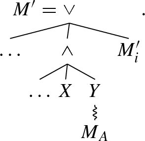
  By semantics of , execution of $M'_i$ does not imply execution of either X or $M_A$. If X is not optional, then execution of $M_A$ implies execution of X, and therefore, $M_A$ and $M'_i$ are not interchangeable ().

  If X is optional, then Y cannot be optional (reduction rule ) and execution of X implies execution of Y. That is, a coo-graph $\alpha _{\text {coo}}(S)'$ that contains $\Sigma (Y)$ and $\Sigma (X)$ would contain the traces $\langle \Sigma (X), \Sigma (Y)) \rangle$ and $\langle \Sigma (X), \Sigma (M'_i), \Sigma (Y) \rangle$ but not $\langle \Sigma (X), \Sigma (M'_i) \rangle$. Therefore, 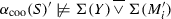. By definition of the occurrence function (“contains any activity of”), .

• The lowest common parent is a parent of $M'$. Then, M contains either of the following structures, for certain nodes X and Y (wiggled edges denote possibly indirect children; $M_A$ may be equivalent to Y):

  

In the first case, X and $M'$ cannot be both optional (reduction rule ). Then, by semantics of $\wedge$, execution of X implies execution of $M'$ (if $M'$ is not optional) and/or execution of $M'$ implies execution of X (if X is not optional). By the reduction rules, there must be an -node or an construct between $\oplus$ and $M'$. Then, execution of neither $M'$ nor X is implied by execution of $M_A$, so .

In the second case, a similar argument holds for Y and $M'$.

Then, by Definition 7.7, is not a partial -cut of $\alpha _{\text {coo}}(S)$.

Hence, is a partial -cut of $\alpha _{\text {coo}}(S)$ if and only if $\exists _{1 \leqslant j \leqslant m}~ A = \Sigma (M'_j)$. $\square$

1.5 Lemma F.3

Lemma: Let $M \in \textsc {C}_{\text {coo}}{}$ be a reduced process tree with a coo-stem, let $M' = \wedge (M'_1, \ldots M'_m)$, $M' \in {{\,\mathrm{coo-stem}\,}}(M)$ be a coo-stem node, let $M'_i$ be a child of $M'$, let $S \in \mathbb {M}^{\Sigma }(M)$ a partition such that $\Sigma (M'_i) \in S$, and let $\alpha _{\text {coo}}(\mathcal {L}(M), S)$ be a coo-graph. Take any $A \in S$ such that $A \ne \Sigma (M'_i)$. Then, $(\wedge , \Sigma (M'_i), A)$ or $(\wedge , A, \Sigma (M'_i))$ is a partial $\wedge$-cut of $\alpha _{\text {coo}}(\mathcal {L}(M), S)$ if and only if $\exists _{1 \leqslant j \leqslant m}~ A = \Sigma (M'_j)$.

Proof

Prove both directions separately:

$\Leftarrow$:

Take such an $M'_j$. By Lemma B.2, $(\wedge , \Sigma (M'_i), A)$ is a partial $\wedge$-cut of $\alpha _{\text {coo}}(S)$.

$\Rightarrow$:

Towards contradiction, assume that there exists a set of activities A such that $(\wedge , \Sigma (M'_i), A)$ is a partial $\wedge$-cut of $\alpha _{\text {coo}}(S)$ and $\forall _{1 \leqslant j \leqslant m}~ A \ne \Sigma (M'_j)$. By Definition F.1, A corresponds to a node in M. Let $M_A$ be this node. Perform case distinction on whether the lowest common parent of $M_A$ and $M'$ is either $M'$ itself or a parent of $M'$:

• The lowest common parent is $M'$. By the assumptions made, $M_A$ is not a direct child of $M'$. Then, M contains either of the following structures, for a certain node X (wiggled edges denote possibly indirect children):

  

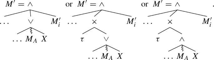
  In all cases, , so $(\wedge , \Sigma (M'_i), A)$ is not a partial $\wedge$-cut of $\alpha _{\text {coo}}(S)$ and the partial cut $(\wedge , A, \Sigma (M_i'))$ must adhere to the second option of Definition 7.8.

  In the first case, if $M'_i$ is not optional, then execution of X implies execution of $M'_i$. Then, for every $Y \in \mathbb {M}^{\Sigma }(X)$, $\alpha _{\text {coo}}(S) \models Y \overline{\Rightarrow }\Sigma (M'_i)$, and at least one such Y is in S, which violates Requirement c.3.4. If $M'_i$ is optional, then , which violates Requirement c.3.2. In the second and third cases, by reduction rule , $M_i'$ cannot be optional, and an argument similar to the first case applies. Hence, $(\wedge , A, \Sigma (M_i'))$ is not a partial $\wedge$-cut of $\alpha _{\text {coo}}(S)$.

• The lowest common parent is a parent of $M'$. Then, M contains either of the following structures, for certain nodes $X_1, X_2, X_4$ (wiggled edges denote possibly indirect children):

  

  In all these cases, , so $(\wedge , A, \Sigma (M'_i))$ is not a partial $\wedge$-cut of $\alpha _{\text {coo}}(S)$ and the partial cut $(\wedge , \Sigma (M_i'), A)$ must adhere to the second option of Definition 7.8.

• In the first case, if $\alpha _{\text {coo}}(S) \models \Sigma (M'_i) \overline{\Rightarrow }A$ then for every $Y \in \mathbb {M}^{\Sigma }(X_1)$ it holds that $\alpha _{\text {coo}}(S) \models Y \overline{\Rightarrow }A$, and at least one such Y is in S, which violates Requirement c.3.4.

• The second case is similar to the first.

• In the third case, 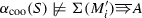, which violates Requirement c.3.2.

• In the fourth case, for every $\alpha _{\text {coo}}(S) \models Y \in \mathbb {M}^{\Sigma }(X_4)$, $Y \overline{\Rightarrow }A$, and one such Y is in S, which violates Requirement c.3.4.

Then, neither $(\wedge , A, \Sigma (M'_i))$ nor $(\wedge , \Sigma (M'_i), A)$ is a partial $\wedge$-cut of $\alpha _{\text {coo}}(S)$.

Hence, $(\wedge , \Sigma (M'_i), A)$ or $(\wedge , A, \Sigma (M'_i))$ is a partial $\wedge$-cut of $\alpha _{\text {coo}}(S)$ if and only if $\exists _{1 \leqslant j \leqslant m}~ A = \Sigma (M'_j)$. $\square$

1.6 Lemma F.7

Lemma: Take two reduced process trees of $\textsc {C}_{\text {coo}}$$K = \oplus (K_1, \ldots K_n)$ and $M = \otimes (M_1, \ldots M_m)$ such that $\oplus \ne \otimes$. Then, $\alpha _{\text {dfg}}(K) \ne \alpha _{\text {dfg}}(M)$ or $\alpha _{\text {coo}}(K) \ne \alpha _{\text {coo}}(M)$.

Proof

Towards contradiction, assume that $\alpha _{\text {dfg}}(K) = \alpha _{\text {dfg}}(M)$ and $\alpha _{\text {coo}}(K) = \alpha _{\text {coo}}(M)$. Perform case distinction on $\oplus$:

• and one child $K_i$ is a $\tau$. As described before, the footprint of applies whenever the root is optional. Thus, we need to consider the case in which M is optional, but does not have the construct as root. Let (or if ) and perform case distinction on $\otimes$:

  • By semantics of , $\alpha _{\text {dfg}}(M)$ consists of unconnected clusters. As $\alpha _{\text {dfg}}(M) = \alpha _{\text {dfg}}(K)$, and by semantics of the operators, . At least one child (say $M_j$) is optional, but does not have the construct as root. Let $K'_i$ be the corresponding child in K. Then, $\mathcal {L}(K'_i) \cup \{\epsilon \} = M_j$. $M_j$ cannot be a single activity (cannot be optional without the construct), or (by Rule  ). For the other operators, see the other cases (termination of the argument guaranteed as $K_i$ and $M_j$ are strictly smaller than M).

  • $\otimes \,=\,\rightarrow$ By semantics of $\rightarrow$, $\alpha _{\text {dfg}}(M)$ consists of a chain of clusters. As $\alpha _{\text {dfg}}(M) = \alpha _{\text {dfg}}(K)$, and by semantics of the operators, $\oplus ' = \rightarrow$. By semantics of $\rightarrow$, all children $M_j$ are optional. By Rule  , at least one child (say $K_i$) is not optional. Therefore, there is a non-empty trace in $\mathcal {L}(K)$ in which no activity of $\Sigma (K_i)$ occurs. There is no such $M_j$, thus $\mathcal {L}(K) \ne \mathcal {L}(M)$.

  • $\otimes \,=\,\wedge$ By semantics of $\wedge$, all children $M_j$ must be optional. However, by Rule  , this situation cannot occur.

  • By semantics of , at least one child $M_j$ is optional. Consider the options for $M_j$ exhaustively: (would be reduced by Rule  ), (would be reduced by Rule  ), $\wedge (\ldots )$ with all children optional (would be reduced by Rule  ), a (cannot be optional without construct), or, hence, an optional non-coo-subtree without as root. For the other operators, see the other cases (termination of the argument guaranteed as $K_i$ and $M_j$ are strictly smaller than M).

  • $\otimes \,=\, \leftrightarrow$ By semantics of the process tree operators, $\oplus ' \,=\, \leftrightarrow$. By reduction rule  , at least one child $K'_i$ is not optional. By Definition 7.9, all children $M_i$ must be optional.

    Take a child $K'_{j \ne i}$. Then, execution of some activity in $K'_j$ implies execution of some activity in $K'_i$, while there can be no child $M_{j \ne i}$ with such a dependency can exist in $M_i$, as $\leftrightarrow$ cannot be nested by Definition 7.9. Hence, $\alpha _{\text {dfg}}(K) \ne \alpha _{\text {dfg}}(M)$.

  • $\otimes \,=\, \circlearrowleft$ In this case, $\circlearrowleft$ is optional and this is excluded by Requirement $\hbox {C}_{\mathrm{coo}}.\hbox {l}.2$.

  Hence, $\alpha _{\text {dfg}}(K) \ne \alpha _{\text {dfg}}(M)$.

• and no child is a $\tau$. The graph $\alpha _{\text {dfg}}(M)$ consists of several unconnected components, while as $\otimes$ is either , $\alpha _{\text {dfg}}(M)$ is connected. Thus, $\alpha _{\text {dfg}}(K) \ne \alpha _{\text {dfg}}(M)$.

• $\oplus = \rightarrow$ The graph $\alpha _{\text {dfg}}(M)$ is a chain, while as $\otimes$ is either , $\alpha _{\text {dfg}}(M)$ is either unconnected or strongly connected. Thus, $\alpha _{\text {dfg}}(K) \ne \alpha _{\text {dfg}}(M)$.

• $\oplus \,=\,\wedge$ We consider the remaining cases of $\otimes$:

  • By Lemma F.5, $\alpha _{\text {dfg}}(M) \ne \alpha _{\text {dfg}}(K)$ or $\alpha _{\text {coo}}(M) \ne \alpha _{\text {coo}}(K)$.

  • $\otimes \,=\, \leftrightarrow$ As shown in Sect. 7.1, optionality does not influence the footprint of $\wedge$ or $\leftrightarrow$. Therefore, Lemma 5.2 applies. Hence, $\alpha _{\text {dfg}}(M) \ne \alpha _{\text {dfg}}(K)$.

  • $\otimes \,=\, \circlearrowleft$ By Definition 7.9, children of $\circlearrowleft$ are not allowed to be optional. Therefore, Lemma 5.2 applies. Hence, $\alpha _{\text {dfg}}(M) \ne \alpha _{\text {dfg}}(K)$.

• has the same directly follows footprint as $\wedge$. Therefore, the arguments given at $\oplus = \wedge , \otimes \,=\,\leftrightarrow$ and $\otimes \,=\,\circlearrowleft$ apply.

• $\oplus \,=\,\leftrightarrow$ We consider the remaining case of $\otimes$, being $\otimes \,=\, \circlearrowleft$.

  By Definition 7.9, children of $\circlearrowleft$ are not allowed to be optional. Therefore, Lemma 5.2 applies. Hence, $\alpha _{\text {dfg}}(M) \ne \alpha _{\text {dfg}}(K)$.

We conclude that $\alpha _{\text {dfg}}(K) \ne \alpha _{\text {dfg}}(M)$ or $\alpha _{\text {coo}}(K) \ne \alpha _{\text {coo}}(M)$. $\square$

1.7 Lemma F.8

Lemma: take two reduced process trees of $\textsc {C}_{\text {coo}}$$K = \oplus (K_1 \ldots K_n)$ and $M = \oplus (M_1 \ldots M_m)$ such that their activity partition is different, i.e. there is a $1 \leqslant w \leqslant n$ such that $\Sigma (K_w) \ne \Sigma (M_w)$. Then, $\alpha _{\text {dfg}}(K) \ne \alpha _{\text {dfg}}(M)$ or $\alpha _{\text {coo}}(K) \ne \alpha _{\text {coo}}(M)$.

Proof

Without loss of generality, we assume a fixed order of subtrees for all operators. Towards contradiction, assume that $\alpha _{\text {dfg}}(K) = \alpha _{\text {dfg}}(M)$ and $\alpha _{\text {coo}}(K) = \alpha _{\text {coo}}(M)$. Perform case distinction on $\oplus$ (the case for K and M swapped is symmetric).

• If a child $K_i$ is $\tau$, see the proof of Lemma F.7.

  As K is reduced, $\alpha _{\text {dfg}}(K)$ contains n unconnected clusters, corresponding to $\Sigma (K_i)$’s. These clusters themselves are connected (by Rule and semantics of the other operators); hence, $\alpha _{\text {dfg}}(K)$ contains a maximal cut. The same holds for $\alpha _{\text {dfg}}(M)$, hence $\Sigma (K_w) = \Sigma (M_w)$.

• $\oplus = \rightarrow$ By Lemma F.1, $\Sigma (K_w) = \Sigma (M_w)$.

• $\oplus = \wedge$ By Lemma F.6, $\Sigma (K_w) = \Sigma (M_w)$.

• $\oplus = \leftrightarrow$ Let $K_w = \otimes (K_{w_1}\ldots K_{w_p})$. Perform case distinction on $\otimes$:

  • and a child $M_i$ is $\tau$. The $\leftrightarrow$ operator has a distinct directly follows graph footprint, on which has no influence. Therefore, refer to the other cases as if $\otimes$ is the child of , using the requirements of $\textsc {C}_{\text {coo}}$.

  • and no child $M_i$ is $\tau$. By semantics of , no end activity of $K_{w_1}$ has a connection to any start activity of any other $K_{w_j}$. Thus, as M contains an interleaved activity partition, $\Sigma (K_w) \subseteq \Sigma (M_w)$.

  • $\otimes =\,\rightarrow$ Similar to the case.

  • $\otimes =\,\wedge$ and . By Definition 7.9, at least one child of $K_w$ has disjoint start and end activities. Take such a child $K_{w_y}$, and consider two activities: $a \notin {{\,\mathrm{Start}\,}}(K_{w_y})$ and $b \in \Sigma (K_w){\setminus }K_{w_y}$. By semantics of $\wedge$ and , $\alpha _{\text {dfg}}(b, a)$. Then, by Lemma 5.1, $a \in \Sigma (M_w)$ and $b \in \Sigma (M_w)$. This holds for all b and by symmetry for ${{\,\mathrm{Start}\,}}(K_{w_y}) \cup {{\,\mathrm{End}\,}}(K_{w_y})$. By semantics of $\leftrightarrow$, non-start non-end activities only have connections with start/end activities of $K_w$. Therefore, $\Sigma (K_w) {\setminus }{}$$({{\,\mathrm{Start}\,}}(K_w) \cup {{\,\mathrm{End}\,}}(K_w))$$\subseteq \Sigma (M_w)$. Hence, $\Sigma (K_w) \subseteq \Sigma (M_w)$.

  • $\otimes \,=\, \leftrightarrow$ Excluded by Definition 7.9.

  • $\otimes \,=\,\circlearrowleft$ By semantics of $\leftrightarrow$, non-start non-end activities only have connections with start/end activities of $K_w$. Therefore, $\Sigma (K_w) \setminus ({{\,\mathrm{Start}\,}}(K_w) \cup {{\,\mathrm{End}\,}}(K_w)) \subseteq \Sigma (M_w)$. All activities $\in {{\,\mathrm{Start}\,}}(K_w) \cup {{\,\mathrm{End}\,}}(K_w)$ have connections from/to ${{\,\mathrm{End}\,}}(K_{w_2}) \cup {{\,\mathrm{Start}\,}}(K_{w_2})$, thus ${{\,\mathrm{Start}\,}}(K_w) \cup {{\,\mathrm{End}\,}}(K_w)$${}\subseteq \Sigma (M_w)$. Hence, $\Sigma (K_w) \subseteq \Sigma (M_w)$.

  By symmetry, $\Sigma (K_w) = \Sigma (M_w)$.

• In K, . By Lemma F.2 and as $\alpha _{\text {dfg}}(K) = \alpha _{\text {dfg}}(M)$ and $\alpha _{\text {coo}}(K) = \alpha _{\text {coo}}(M)$, it holds that . Hence, $\Sigma (K_w) = \Sigma (M_w)$.

• $\oplus = \circlearrowleft$ By Definition 7.9, children of $\circlearrowleft$ are not allowed to be optional. Therefore, Lemma 5.3 applies.

By contradiction, we conclude that $\alpha _{\text {dfg}}(K) \ne \alpha _{\text {dfg}}(M)$ or $\alpha _{\text {coo}}(K) \ne \alpha _{\text {coo}}(M)$. $\square$

References

van der Aalst WMP (2016) Process mining–data science in action, 2nd edn. Springer, Berlin. https://doi.org/10.1007/978-3-662-49851-4
Buijs JCAM, van Dongen BF, van der Aalst WMP (2014) Quality dimensions in process discovery: the importance of fitness, precision, generalization and simplicity. Int J Cooperative Inf Syst. https://doi.org/10.1142/S0218843014400012
van der Aalst WMP, Weijters AJMM, Maruster L (2004) Workflow mining: discovering process models from event logs. IEEE Trans Knowl Data Eng 16:1128–1142
vanden Broucke SKLM, Weerdt JD (2017) Fodina: a robust and flexible heuristic process discovery technique. Decis Support Syst 100:109–118
Leemans SJJ, Fahland D, van der Aalst WMP (2013) Discovering block-structured process models from event logs—a constructive approach. In: PETRI NETS 2013. Lecture notes in computer science, vol 7927. Springer, pp 311–329. https://doi.org/10.1007/978-3-642-38697-8_17
Augusto A, Conforti R, Dumas M, Rosa ML (2017) Split miner: discovering accurate and simple business process models from event logs. In: ICDM 2017. IEEE Computer Society, pp 1–10. https://doi.org/10.1109/ICDM.2017.9
Weidlich M, van der Werf JMEM (2012) On profiles and footprints—relational semantics for petri nets. In: Petri Nets
Polyvyanyy A, Armas-Cervantes A, Dumas M, García-Bañuelos L (2016) On the expressive power of behavioral profiles. Form Asp Comput 28:597–613
Leemans SJJ, Fahland D, van der Aalst WMP (2014) Discovering block-structured process models from event logs containing infrequent behaviour. In: Lohmann N, Song M, Wohed P (eds) Business process management workshops. Lecture notes in business information processing, vol 171. Springer, pp 66–78
Augusto A, Conforti R, Dumas M, Rosa ML, Maggi FM, Marrella A, Mecella M, Soo A (2018) Automated discovery of process models from event logs: review and benchmark. IEEE Trans Knowl Data Eng. arXiv:1705.02288
OMG (2011) Business Process Model and Notation (BPMN), Version 2.0. http://www.omg.org/spec/BPMN/2.0. Accessed 8 July 2019
van Zelst SJ, van Dongen BF, van der Aalst WMP (2018) Event stream-based process discovery using abstract representations. Knowl Inf Syst 54(2):407–435. https://doi.org/10.1007/s10115-017-1060-2
Syamsiyah A, van Dongen BF, van der Aalst WMP (2016) DB-XES: enabling process discovery in the large. In: SIMPDA 2016. LNBIP, vol 307. Springer, pp 53–77. https://doi.org/10.1007/978-3-319-74161-1_4
Syamsiyah A, van Dongen BF, van der Aalst WMP (2017) Recurrent process mining with live event data. In: BPM Workshops 2017. LNBIP, vol 308. Springer, pp 178–190
Weerdt JD, Backer MD, Vanthienen J, Baesens B (2012) A multi-dimensional quality assessment of state-of-the-art process discovery algorithms using real-life event logs. Inf Syst 37:654–676
Badouel E, Bernardinello L, Darondeau P (2015) Petri net synthesis. Springer, Berlin
de Medeiros, AKA, van Dongen BF, van der Aalst WMP, Weijters AJMM (2004) Process mining for ubiquitous mobile systems: an overview and a concrete algorithm. In: Baresi L, Dustdar S, Gall HC, Matera M (eds) Ubiquitous mobile information and collaboration systems, second CAiSE workshop, UMICS 2004, Riga, Latvia, 7–8 June 2004, Revised selected papers. Lecture notes in computer science, vol 3272. Springer, pp 151–165. https://doi.org/10.1007/978-3-540-30188-2_12
Wen L, Wang J, Sun J (2006) Detecting implicit dependencies between tasks from event logs. In: Zhou X, Li J, Shen HT, Kitsuregawa M, Zhang Y (eds) Frontiers of WWW Research and Development—APWeb 2006, 8th Asia-Pacific Web Conference, Harbin, China, 16–18 January 2006, Proceedings. Lecture notes in computer science, vol 3841. Springer, pp 591–603. https://doi.org/10.1007/11610113_52
Wen L, van der Aalst WMP, Wang J, Sun J (2007) Mining process models with non-free-choice constructs. Data Min Knowl Discov 15(2):145–180. https://doi.org/10.1007/s10618-007-0065-y
Wen L, Wang J, van der Aalst WMP, Huang B, Sun J (2010) Mining process models with prime invisible tasks. Data Knowl Eng 69(10):999–1021. https://doi.org/10.1016/j.datak.2010.06.001
Wen L, Wang J, Sun J (2007) Mining invisible tasks from event logs. In: Dong G, Lin X, Wang W, Yang Y, Yu JX (eds) Advances in data and web management, Joint 9th Asia-Pacific Web Conference, APWeb 2007, and 8th international conference, on web-age information management, WAIM 2007, Huang Shan, China, 16–18 June 2007, Proceedings. Lecture notes in computer science, vol 4505. Springer, pp 358–365. https://doi.org/10.1007/978-3-540-72524-4_38
Guo Q, Wen L, Wang J, Yan Z, Yu PS (2015) Mining invisible tasks in non-free-choice constructs. In: Motahari-Nezhad HR, Recker J, Weidlich M (eds) Business process management—13th international conference, BPM 2015, Innsbruck, Austria, August 31–September 3 2015, Proceedings. Lecture notes in computer science, vol 9253. Springer, pp 109–125. https://doi.org/10.1007/978-3-319-23063-4_7
Leemans SJJ, Fahland D, van der Aalst WMP (2014) Discovering block-structured process models from incomplete event logs. In: Ciardo G, Kindler E (eds) Application and theory of petri nets and concurrency—35th international conference, PETRI NETS 2014, Tunis, Tunisia, 23–27 June 2014. Proceedings. Lecture notes in computer science, vol 8489. Springer, pp 91–110. https://doi.org/10.1007/978-3-319-07734-5_6
Russell N, van der Aalst WMP, ter Hofstede AHM (2016) Workflow patterns: the definitive guide. MIT Press, Cambridge
Zha H, Wang J, Wen L, Wang C, Sun JG (2010) A workflow net similarity measure based on transition adjacency relations. Comput Ind 61:463–471
Sun J, Gu T, Qian J (2017) A behavioral similarity metric for semantic workflows based on semantic task adjacency relations with importance. IEEE Access 5:15609–15618
van Dongen BF, Dijkman RM, Mendling J (2008) Measuring similarity between business process models. In: CAiSE 2008. Lecture notes in computer science, vol 5074. Springer, pp 450–464. https://doi.org/10.1007/978-3-540-69534-9_34
Polyvyanyy A, Weidlich M Conforti R, Rosa ML, ter Hofstede AHM (2014) The 4c spectrum of fundamental behavioral relations for concurrent systems. In: Petri Nets
Wang J, He T, Wen L, Wu N, ter Hofstede AHM, Su J (2010) A behavioral similarity measure between labeled petri nets based on principal transition sequences—(short paper). In: OTM 2010. Lecture notes in computer science, vol 6426. Springer, pp 394–401
Becker M, Laue R (2012) A comparative survey of business process similarity measures. Comput Ind 63(2):148–167
Kunze M, Weidlich M, Weske M (2011) Behavioral similarity—a proper metric. In: Business process management 2011. Lecture Notes in Computer Science, vol 6896. Springer, pp 166–181
Kunze M, Weidlich M, Weske M (2015) Querying process models by behavior inclusion. Softw Syst Model 14(3):1105–1125. https://doi.org/10.1007/s10270-013-0389-6
Polyvyanyy A, Weidlich M, Weske M (2012) Isotactics as a foundation for alignment and abstraction of behavioral models. In: BPM
Weidlich M, Mendling J, Weske M (2012) Propagating changes between aligned process models. J Syst Softw 85:1885–1898
van der Werf JMEM, van Dongen BF, Hurkens CAJ, Serebrenik A (2009) Process discovery using integer linear programming. Fundam Inf 94(3–4):387–412. https://doi.org/10.3233/FI-2009-136
Schunselaar DMM, Verbeek E, van der Aalst WMP, Reijers HA (2013) A framework for efficiently deciding language inclusion for sound unlabelled wf-nets. In: Joint proceedings of the international workshop on petri nets and software engineering (PNSE’13) and the international workshop on modeling and business environments (ModBE’13), Milano, Italy, 24–25 June 2013. CEUR Workshop Proceedings, vol 989. CEUR-WS.org, pp 135–154
Leemans SJJ, Fahland D, van der Aalst WMP (2018) Scalable process discovery and conformance checking. Softw Syst Model 17(2):599–631. https://doi.org/10.1007/s10270-016-0545-x
Buijs JCAM, van Dongen BF, van der Aalst WMP (2012) A genetic algorithm for discovering process trees. In: Proceedings of the IEEE congress on evolutionary computation, CEC 2012, Brisbane, Australia, 10–15 June. IEEE, pp 1–8. https://doi.org/10.1109/CEC.2012.6256458
Molka T, Redlich D, Gilani W, Zeng X, Drobek M (2015) Evolutionary computation based discovery of hierarchical business process models. In: Abramowicz W (ed) Business information systems—18th international conference, BIS 2015, Poznań, Poland, 24–26 June 2015, Proceedings. Lecture notes in business information processing, vol 208. Springer, pp 191–204. https://doi.org/10.1007/978-3-319-19027-3_16
Leemans SJJ (2017) Robust process mining with guarantees. Ph.D. thesis, Eindhoven University of Technology
Polyvyanyy A, Vanhatalo J, Völzer H (2010) Simplified computation and generalization of the refined process structure tree. In: Bravetti M, Bultan T (eds) Web services and formal methods—7th international workshop, WS-FM 2010, Hoboken, NJ, USA, 16–17 September 2010. Revised Selected Papers. Lecture notes in computer science, vol 6551. Springer, pp 25–41. https://doi.org/10.1007/978-3-642-19589-1_2
Reisig W (1985) Petri nets: an introduction. Springer, New York
Gallo G, Longo G, Pallottino S (1993) Directed hypergraphs and applications. Discrete Appl Math 42(2):177–201. https://doi.org/10.1016/0166-218X(93)90045-P
Conforti R, Rosa ML, ter Hofstede AHM (2017) Filtering out infrequent behavior from business process event logs. IEEE Trans Knowl Data Eng 29(2):300–314. https://doi.org/10.1109/TKDE.2016.2614680
Leemans SJ, Fahland, D (2019) dfahland/exp-abstractions-in-pm-KAIS: original experiment. https://doi.org/10.5281/zenodo.3243981
Leemans SJJ, Fahland D (2019) Process models obtained from event logs with different information-preserving abstractions. https://doi.org/10.5281/zenodo.3243988
van Dongen B (2012) BPI challenge 2012 dataset. https://doi.org/10.4121/uuid:3926db30-f712-4394-aebc-75976070e91f
Acknowledgements
We thank Wil van der Aalst for his contribution to earlier versions of the directly follows and minimum self-distance abstractions [5]. Furthermore, we thank Alifah Syamsiyah for her corrections in the examples of the minimum self-distance abstraction.
Author information
Authors and Affiliations
Corresponding author
Additional information
Publisher's Note
Springer Nature remains neutral with regard to jurisdictional claims in published maps and institutional affiliations.