
Abstract
Domain adaptation (DA) is a new learning framework dealing with learning problems where the target test data are drawn from a distribution different from the one that has generated the learning source data. In this article, we introduce self-labeling domain adaptation boosting (SLDAB), a new DA algorithm that falls both within the theory of DA and the theory of Boosting, allowing us to derive strong theoretical properties. SLDAB stands in the unsupervised DA setting where labeled data are only available in the source domain. To deal with this more complex situation, the strategy of SLDAB consists in jointly minimizing the empirical error on the source domain while limiting the violations of a natural notion of pseudo-margin over the target domain instances. Another contribution of this paper is the definition of a new divergence measure aiming at penalizing models that induce a large discrepancy between the two domains, reducing the production of degenerate models. We provide several theoretical results that justify this strategy. The practical efficiency of our model is assessed on two widely used datasets.
1 Introduction
In the classic machine learning setting, training and test data are supposed to come from the same statistical distribution. However, it is worth noting that this assumption does not hold in many real applications challenging common learning theories such as the PAC model [44]. To cope with such situations, a new machine learning framework has been recently studied leading to the emergence of the theory of domain adaptation (DA) [5, 29]. A standard DA problem can be defined as a situation where the learner receives labeled data drawn from a source domain (or even from several sources [28]) and very few or no labeled points from the target distribution. DA arises in a large spectrum of applications, such as in computer vision [32], speech processing [26, 38], natural language processing [8, 12], etc. During the past few years, new fundamental results opened the door for the design of theoretically well-founded DA algorithms. In this paper, we focus on the scenario where the training set is made of labeled source data and unlabeled target instances. To deal with this more complex situation, several solutions have been presented in the literature (see, e.g., surveys [31, 37]). Among them, instance weighting-based methods are used to deal with covariate shift where the labeling functions are supposed to remain unchanged between the two domains. On the other hand, feature representation approaches aim at seeking a domain invariant feature space by either generating latent variables or selecting a relevant subset of the original features. A third class of approaches, called iterative self-labeling methods, consists in iteratively inserting target examples, which have been labeled, in the learning set.
In this paper, our objective is to propose a new approach, taking advantage of both feature representation and iterative self-labeling approaches. The idea is to iteratively learn a large margin linear hyperplane in a new projection space. We present a novel DA algorithm which takes its origin from both the theory of boosting [17] and the theory of DA. Let us remind that boosting (via its well known AdaBoost algorithm) iteratively builds a combination of weak classifiers. At each step, AdaBoost makes use of an update rule which increases (resp. decreases) the weight of those instances misclassified (resp. correctly classified) by previous classifiers. It is worth noting that boosting has already been exploited in DA methods but mainly in supervised situations where the learner receives some labeled target instances. In [13], TrAdaBoost uses the standard weighting scheme of AdaBoost on the target data, while the weights of the source instances are monotonically decreased according to their margin. A generalization of TrAdaBoost to multiple sources is presented in [50]. On the other hand, some boosting-based approaches relax the constraint of having labeled target examples. However, they are proposed in the context of semi-supervised ensemble methods, i.e. assuming that the source and the target domains are (sufficiently) similar [6, 27].
In this paper, we present self-labeling domain adaptation boosting (SLDAB), a boosting-like DA algorithm which both optimizes the source classification error and margin constraints over the unlabeled target instances. However, unlike state of the art self-labeling DA methods, SLDAB aims at also reducing the divergence between the two distributions in the space of the learned hypotheses. In this context, we introduce the notion of weak DA assumption which takes into account a measure of divergence. This classifier-induced measure is exploited in the update rule so as to penalize hypotheses inducing a large discrepancy. This strategy tends to prevent the algorithm from building degenerate models which would, e.g., perfectly classify the source data while moving the target examples far away from the learned hyperplane (and thus satisfying any margin constraint). We present a theoretical analysis of SLDAB and derive several theoretical results that, in addition to good experimental results, support our claims.
The rest of this paper is organized as follows: after an overview on related work in DA in Sect. 2 and an intuition about our work in Sect. 3; we give notations and definitions in Sect. 4. SLDAB is presented in Sect. 5 and theoretically analyzed in Sect. 6. We then discuss the way to compute the divergence between the source and target domains in Sect. 7. Finally, we conduct two series of experiments and show practical evidences of the efficiency of SLDAB in Sect. 8, before discussing about generalization guarantees in Sect. 9 and concluding in Sect. 10.
2 Related work in domain adaptation
We consider the binary classification problem in which we have a training set \(S \cup T\) with \(S\) a set of labeled data \((x',y')\) drawn from a source distribution \(\mathcal{S}\) over \(Z= X \times Y\), where \(X\) is the instance space and \(Y=\{-1,+1\}\) is the set of labels and \(T\) a set of unlabeled examples \(x\) drawn from a target distribution \(\mathcal{T}\) over \(X\). We want to learn a classifier with an error rate \(\epsilon _\mathcal{T}\) as low as possible over the target distribution. In this setting, the (unknown) generalization source error of a hypothesis \(h \in \mathcal{H}\) is defined as follows:
where \(\ell :\mathcal{H} \times X \times \{-1,+1\} \rightarrow \mathbb {R}^+\) is a nonnegative loss function, while the (unknown) generalization target error of \(h\) is:
2.1 Theoretical results in DA
In the past few years, DA has been widely studied from a statistical learning theory point of view. Typically, these theoretical results take the form of upper bounds on the generalization target error of \(h\), which has been learned from the source data. To assess the adaptation difficulty of a given problem at hand, Ben-David et al. introduce in [5] the \(\mathcal {H} \Delta \mathcal {H}\)-divergence, noted \(d_{\mathcal {H} \Delta \mathcal {H}}(\mathcal {S},\mathcal {T})\), which is a measure between the source and the target distributions w.r.t. \(\mathcal {H}\). To estimate this divergence, the authors suggest to label each source example of \(S\) with \(-1\) and each unlabeled example of \(T\) as \(+1\) and train a classifier to discriminate between source and target data. The \(\mathcal {H} \Delta \mathcal {H}\)-divergence is immediately computable from the error of the classifier and a term of complexity which depends on the Vapnik–Chervonenkis dimension (VC-dim) of the hypothesis space. Intuitively, if the error is low, we are thus able to easily separate source and target data that means that the two distributions are quite different. On the other hand, the higher the error, the less different \(\mathcal {S}\) and \(\mathcal {T}\). The authors provide a generalization bound for domain adaptation on \(\epsilon _{T}(h)\) which generalizes the standard bound on \(\epsilon _{S}(h)\) by taking into account the \(\mathcal {H} \Delta \mathcal {H}\)-divergence between the source and target distributions. More formally:
where \(\lambda \) is the error of the ideal joint hypothesis on the source and target domains (which is supposed to be a negligible term if the adaptation is possible). Equation (1) expresses the idea that to adapt well, the DA algorithm has to learn an hypothesis \(h\) which works well on the source data while reducing the divergence between \(\mathcal {S}\) and \(\mathcal {T}\).
Based on this work, Mansour et al. [29] introduce a new divergence measure called discrepancy distance. Its empirical estimate is based on the Rademacher [3, 25] complexity (rather than the VC-dim) allowing the use of arbitrary loss functions leading to generalization bounds useful for more general learning problems, such as in classification with SVMs or in regression.
There also exists other theoretical works that have been made in the field of DA, such as [30], which takes advantage of the robustness properties introduced in [46, 48], together with the notion of \(\lambda \)-shift between two distributions, to derive generalization bounds on the target error.
2.2 Algorithmic contributions
Following the underlying ideas of Eq. (1), many DA algorithms have been proposed in the literature in different settings. We present in the following some of these approaches (for more details, the interested reader may refer to the following surveys [22, 31, 35]).
2.2.1 Instance weighting
When the training examples, drawn in a biased manner, are not representative enough of \(\mathcal {T}\), we have to face a problem of sample selection bias. Covariate shift describes the sample selection bias scenario where the prior distributions \(P_\mathcal{S}(x)\) and \(P_\mathcal{T}(x)\) differ but the conditional probabilities are the same, i.e. \(P_\mathcal{S}(y|x) = P_\mathcal{T}(y|x)\).
Assuming that a certain mass of the source data can be used for learning the target examples, the domain adaptation can be done by resorting to a reweighting scheme of the data. Some solutions have been proposed (e.g., see [20, 42]) that use the ratio of the test and training input densities. Roughly speaking, the idea is to increase the importance of source points located into a region where there is a high density of target points. A learning process is then launched on this reweighted training set, which is supposed to be much closer from the target distribution than the unweighted one. In [15], the sample selection bias is corrected by resorting to an entropy maximization, while in [43], the source data are reweighted while minimizing the Kullback–Leibler-divergence between the source and target distributions. Finally, in [7], a classifier is found as the solution of an optimization problem integrating the covariate shift problem.
2.2.2 New feature representations
Rather than reweighting the source data, another way to handle DA problems consists in changing the feature representation of the data to better describe shared characteristics of the two domains \(\mathcal {S}\) and \(\mathcal {T}\). We distinguish two different strategies: the first one assumes that some features are generalizable, and thus they can be shared by both domains, while some others are domain-specific. In this context, a feature selection algorithm which penalizes or removes some features can be used to find the shared low-dimensional space. In [39], the authors suggest to train a model maximizing the likelihood over the training sample on a subset of the original features, minimizing the distance between the two distributions. Another approach proposed in [4] tries to find a task-independent decision boundary in a common space thanks to a nonlinear mapping of the features in each task. This methods stands rather in a multi-task setting and requires labeled examples in each task, and thus target labels in a two tasks setting.
The second strategy aims at learning new latent features. For example, Florian et al. [16] proposed an algorithm that builds a model on the source domain and uses the predicted labels as new features for both source and target data. In [9], the authors introduce the notion of Structural Correspondence Learning (SCL). They identify the correspondence between features of the two domains by modeling their correlations. In this case, the principle is to project the examples from both domains into the same low-dimensional space, obtained by a mapping of the original features as done for example with a Principal Component Analysis (PCA). In [21], the authors use SCL in a Multi-View way. They first choose \(m\) bridge features, as does SCL and then learn for each domain a correspondence between these bridge features and the other features. Finally, a Multi-View Principal Component Analysis is applied to learn a low-dimensional space. In [14], a mapping is learned from the original \(n\)-dimensional space to a new \(3n\)-dimensional space, where the first \(n\) features are shared by both domains, and the last \(n+n\) features are specific to the source and target domains respectively. Note that in this work, the author makes use of a small but labeled set of target data.
Finally, a recent work by [33, 34] tries to minimize the \(\mathcal {H}\)-divergence in order to decrease the generalization target error. The authors propose an approach based on the recent theory of (\(\varepsilon ,\gamma ,\tau \))-good similarity functions [1, 2], which aims to project examples in a new space where each dimension represents the similarity to a learning example.
2.2.3 Iterative Self-labeling
In order to take advantage of the available unlabeled target data during the learning process, iterative self-labeling methods use and label some of them with an hypothesis built from source examples. Such target data are usually called semi-labeled examples. Then, a new classifier is trained taking into account these semi-labeled data, thus considering information from both domains. The main difficulty is to define the way of choosing the considered target points (and the appropriate proportion). Intuitively, a good strategy would retain the semi-labeled target data for which we have the greater confidence in their classification. Perez et al. [36] introduce a two-step algorithm: first, a statistical model is learned from the source domain. Then, using an extension of the EM algorithm, they estimate how these source parameters change in the target set. The assumption is that large changes are less likely to occur than small ones. Finally, they use this re-estimated model to learn a classifier for the target domain. Other works have been proposed, based on co-training or self-training methods [10].
The most famous self-labeling algorithm is certainly DASVM, introduced in [11], and which was shown to be very competitive. The idea is to iteratively incorporate target samples from \(T\) into the learning set to progressively modify an SVM classifier \(h\). Despite good practical results, DASVM is not theoretically founded. In a recent work, [18] has been proposed a theoretical analysis on the necessary conditions ensuring the good behavior of a self-labeling process. An algorithm is also introduced, using the (\(\varepsilon ,\gamma ,\tau \))-good similarity functions [1, 2], and specifically designed for an application on structured data.
In this paper, we try to take advantage of two categories of approaches in the same time, by introducing an algorithm, SLDAB, which follows an iterative procedure by learning weak classifiers with the help of target examples and finally combines all theses weak hypotheses to obtain a hyperplane in a new space in which are projected both source and target data. We give an intuition on our algorithm in the next section.
3 Intuition behind SLDAB
Let us recall that boosting aims to iteratively learn weak classifiers \(h_n\) (typically, stumps) and to make a linear combinations of all the classifiers regarding their relevance. In the classic supervised classification setting, this relevance depends on the ability of \(h_n\) to correctly label source examples from the training set \(S\) drawn according to the current distribution \(D_n^S\). As a recall, the final classifier \(F^N_S\), after \(N\) iterations, is defined as follows:
where \(\alpha _n = \frac{1}{2}\ln \frac{1-\hat{\epsilon }_n(h_n)}{\hat{\epsilon }_n(h_n)},\) and \(\hat{\epsilon }_n=\mathbb {E}_{(x,y) \sim D_n^S}[\ell (h,(x,y))].\)
In a geometric way, \(F^N_S\) takes the form of an optimized hyperplane in the space corresponding to the outputs of the classifiers \(h_n\).
In the DA setting, the adaptation of boosting is not straightforward. Indeed, the learning set is made not only of a subset \(S\) of labeled source examples, but it also contains a subset \(T\) made of unlabeled target samples. In this paper, we aim to use the same weak learners to minimize both the empirical error on \(S\) while maximizing the margins on \(T\). This strategy consists in projecting both source and target examples in the same \(N\)-dimensional space (\(N\) still being the number of iterations of the algorithm), while reducing the divergence between the two domains in this new space.
If the learned hypotheses \(h_1,\ldots ,h_n,\ldots ,h_N\) are the same for \(S\) and \(T\), note that we aim to optimize different weighting coefficients depending on the domain the example belongs to. Indeed, if it seems natural (and theoretically founded) to keep minimizing the empirical classification error on the labeled source examples, a different strategy has to be applied on the target data for which we do not have access to the labels. We claim that the quality of an hypothesis \(h_n\) on the examples from \(T\) has to depend on its ability to minimize the proportion of margin violations of the target examples. Therefore, our objective is to optimize a second linear combination \(\displaystyle F^N_T = \sum \nolimits _{n=1}^N \beta _n h_n(\mathbf {x})\), where \(\beta _n\) depends both on the example margin and the divergence between \(S\) and \(T\) induced by \(h_n\).
In this context, SLDAB aims to jointly learn two separator hyperplanes in the same \(N\)-dimensional space, common to source and target examples. The geometrical orientation of \(F^N_S\) and \(F^N_T\) will depend on their ability to minimize respectively the empirical classification error on \(S\) and the proportion of margin violations on \(T\). Figure 1 illustrates this idea.

Illustration of the intuition behind SLDAB on the Moons database where the target data are generated after a rotation of the source examples. Source and target examples are projected in the same \(N\)-dimensional space, where the same \(N\) weak hypotheses are combined to get the final classifier. The only difference is about the weights applied in the combination. For the source domain \(S\) (on the left), the \(\alpha \)’s parameters are optimized w.r.t. the classification error on \(S\), while for the target distribution \(T\) (on the right), the \(\beta \)’s parameters are learned w.r.t. the ability of the hypothesis to maximize the margins
As previously stated, minimizing the classification error on \(S\) and maximizing the margins on \(T\) is not sufficient. Indeed, designing an algorithm only dedicated to optimize these two criteria may lead to degenerate situations as illustrated in Fig. 2. We can see that along the iterations the algorithm tends to increase the divergence between \(S\) and \(T\) by moving away source and target data, while minimizing source classification errors and target margin violations. This justifies the need of taking into account a divergence measure, depending on the specific hypothesis \(h_n\), to prevent us from getting degenerate situations. In the next four sections, we consider a generic definition of the divergence. We specifically focus on this divergence in Sect. 7.

Illustration of the situation caused by degenerate hypotheses. a Describes the situation after the first iteration. If no divergence measure is taken into account during the process, we might face a situation illustrated by b, where the conditions are fulfilled (low source classification error and important target margins), but in which the divergence between the source and target distributions is higher and higher
4 Definitions and notations
Let us recall that we dispose of a set \(S\) of labeled data \((x',y')\) drawn from a source distribution \(\mathcal{S}\) over \(Z=X \times Y\), where \(X\) is the instance space and \(Y=\{-1,+1\}\) is the set of labels, together with a set \(T\) of unlabeled examples \(x\) drawn from a target distribution \(\mathcal{T}\) over \(X\). Let \(\mathcal{H}\) be a class of hypotheses and \(h_n \in \mathcal{H}:X \rightarrow [-1,+1]\) a hypothesis learned from \(S\) and \(T\) and their associated empirical distribution \(D_n^S\) and \(D_n^T\).
We denote by \(g_n \in [0,1]\) a measure of divergence induced by \(h_n\) between \(S\) and \(T\). Our objective is to take into account \(g_n\) in our new boosting scheme so as to penalize hypotheses that do not allow the reduction in the divergence between \(S\) and \(T\). To do so, we consider the function \(f_{DA}: [-1,+1] \rightarrow [-1,+1]\) such that \(f_{DA}(h_n(x)) = |h_n(x)| - \lambda g_n\), where \(\lambda \in [0,1]\). \(f_{DA}(h_n(x))\) expresses the ability of \(h_n\) to not only induce large margins (a large value for \(|h_n(x)|\)), but also to reduce the divergence between \(S\) and \(T\) (a small value for \(g_n\)). \(\lambda \) plays the role of a trade-off parameter between the importance of the margin and the divergence.
Let \(T_n^-=\{x \in T|f_{DA}(h_n(x)) \le \gamma \}.\) If \(x \in T_n^- \Leftrightarrow |h_n(x)| \le \gamma +\lambda g_n\). Therefore, \(T_n^-\) corresponds to the set of target points that either violate the margin condition (indeed, if \(|h_n(x)| \le \gamma \Rightarrow |h_n(x)| \le \gamma +\lambda g_n\)) or do not satisfy sufficiently that margin to compensate a large divergence between \(S\) and \(T\) (i.e. \(|h_n(x)| > \gamma \) but \(|h_n(x)| \le \gamma +\lambda g_n\)). In the same way, we define \(T_n^+=\{x \in T|f_{DA}(h_n(x)) > \gamma \}\) such that \(T=T_n^- \cup T_n^+\). Finally, from \(T_n^-\) and \(T_n^+\), we define \(\displaystyle W_n^+=\sum \nolimits _{x \in T_n^+}D_n^T(x)\) and \(\displaystyle W_n^-=\sum \nolimits _{x \in T_n^-}D_n^T(x)\) such that \(W_n^++W_n^-=1\).
Let us remind that the weak assumption presented in [17] states that a classifier \(h_n\) is a weak hypothesis over \(S\) if it performs at least a little bit better than random guessing, that is \(\hat{\epsilon }_n < \frac{1}{2}\), where \(\hat{\epsilon }_n\) is the empirical error of \(h_n\) over \(S\) w.r.t. \(D_n^S\). In this paper, we extend this weak assumption to the DA setting.
Definition 1
(Weak DA Learner) A classifier \(h_n\) learned at iteration \(n\) from a labeled source set \(S\) drawn from \(\mathcal{S}\) and an unlabeled target set \(T\) drawn from \(\mathcal{T}\) is a weak DA learner for \(T\) if \(\forall \gamma \le 1\):
-
1.
\(h_n\) is a weak learner for \(S\), i.e. \(\hat{\epsilon }_n < \frac{1}{2}\).
-
2.
\(\hat{L}_{n}=\mathbb {E}_{x \sim D_n^T}[|f_{DA}(h_n(x))| \le \gamma ] = W_n^- < \frac{\gamma }{\gamma +max(\gamma ,\lambda g_n)}\).
Condition 1 means that to adapt from \(\mathcal{S}\) to \(\mathcal{T}\) using a boosting scheme, \(h_n\) must learn something new at each iteration about the source labeling function. Condition 2 takes into account not only the ability of \(h_n\) to satisfy the margin \(\gamma \) but also its capacity to reduce the divergence between \(S\) and \(T\). From Definition 1, it turns out that:
-
1.
if \(max(\gamma ,\lambda g_n)=\gamma \), then \(\frac{\gamma }{\gamma +max(\gamma ,\lambda g_n)}=\frac{1}{2}\) and Condition 2 looks like the weak assumption over the source, except the fact that \(\hat{L}_{n}<\frac{1}{2}\) expresses a margin condition, while \(\hat{\epsilon }_n < \frac{1}{2}\) considers a classification constraint. Note that if this is true for any hypothesis \(h_n\), it means that the divergence between the source and target distributions is rather small, and thus the underlying task looks more like a semi-supervised problem.
-
2.
if \(max(\gamma ,\lambda g_n)=\lambda g_n\), then the constraint imposed by Condition 2 is stronger (that is \(\hat{L}_{n}<\frac{\gamma }{\gamma +max(\gamma ,\lambda g_n)} < \frac{1}{2}\)) in order to compensate a large divergence between \(S\) and \(T\). In this case, the underlying task requires a domain adaptation process in the weighting scheme.
In the following, we make use of this weak DA assumption to design a new boosting-based DA algorithm, called SLDAB.

5 SLDAB algorithm
The pseudo-code of SLDAB is presented in Algorithm 1. Starting from uniform distributions over \(S\) and \(T\), it iteratively learns a new hypothesis \(h_n\) that verifies the weak DA assumption of Definition 1. Note that this task is not trivial. Indeed, while learning a stump (i.e. a one-level decision tree) is sufficient to satisfy the weak assumption of AdaBoost, finding an hypothesis fulfilling Condition 1 on the source and Condition 2 on the target is more complex. To overcome this problem, we present in the following a simple strategy which tends to induce hypotheses that satisfy the weak DA assumption.
First, we generate \(\frac{k}{2}\) stumps that satisfy Condition 1 over the source and \(\frac{k}{2}\) that fulfill Condition 2 over the target. Then, we seek a convex combination \(\displaystyle h_n=\sum \nolimits _k \kappa _k h_n^k\) of the \(k\) stumps that satisfies simultaneously the two conditions of Definition 1. To do so, we propose to solve the following convex optimization problem:
where \([1-x]_+=max(0,1-x)\) is the hinge loss. Solving this optimization problem tends to fulfill Definition 1. Indeed, minimizing the first term of Eq. (2) tends to reduce the empirical risk over the source data, while minimizing the second term tends to decrease the number of margin violations over the target data. Using the combination of several stumps thus allows us to satisfy the two conditions, as illustrated in Fig. 3.

Illustration of the stumps combination. A single stump would not be sufficient to satisfy the two conditions of Definition 1. This explains why we propose to combine several of them, as illustrated in this figure, where the combination of \(h_n^1\) and \(h_n^2\) allows us to obtain a weak learner for Domain Adaptation, correctly classifying most of the source examples and achieving in the same time large margins, with respect to \(\gamma \) and \(\lambda g_n\), on the target domain
Note that in order to generate a simple weak DA learner, we start the process with \(k=2\). If the optimized combination does not satisfy the weak DA assumption, we draw a new set of \(k\) stumps. If the weak DA assumption is not satisfied after several tries, we increase the dimension of the induced hypothesis \(h_n\). If despite the increase of \(k\) (limited to a given value), no hypothesis is able to fulfill the DA weak learner conditions, the adaptation is stopped. The pseudo-code of the algorithm seeking for weak DA hypotheses is described in Algorithm 2.

Once \(h_n\) has been learned, the weights of the labeled and unlabeled data are modified according to two different update rules. Those of source examples are updated using the same strategy as that of AdaBoost. Regarding the target examples, their weights are changed according to their location in the space. If a target example \(x\) does not satisfy the condition \(f_{DA}(h_n(x)) > \gamma \), a pseudo-class \(y^n=-sgn(f_{DA}(h_n(x)))\) is assigned to \(x\) that simulates a misclassification. Note that such a decision has a geometrical interpretation: it means that we exponentially increase the weights of the points located in an extended margin band of width \(\gamma + \lambda g_n\). If \(x\) is outside this band, a pseudo-class \(y^n=sgn(f_{DA}(h_n(x)))\) is assigned leading to an exponential decrease of \(D^T_n(x)\) at the next iteration.
6 Theoretical analysis
In this section, we present a theoretical analysis of our approach. First, we derive a generalization bound on the loss empirically minimized in Algorithm 2. This bound is deduced from the proof of the algorithmic robustness of this algorithm. Then, we focus on theoretical guarantees of SLDAB. Recall that the goodness of a hypothesis \(h_n\) is measured by its ability not only to correctly classify the source examples but also to classify the unlabeled target data with a large margin w.r.t. the classifier-induced divergence \(g_n\). Provided that the weak DA constraints of Definition 1 are satisfied, the standard results of AdaBoost still hold on \(\mathcal{S}\) (because of Condition 1). In the following, we show that the loss \(\hat{L}_{H_N^T}\), which represents after \(N\) iterations the proportion of margin violations over \(T\) (w.r.t. the successive divergences \(g_n\)), also decreases with \(N\).
6.1 Consistency guarantees of Algorithm 2
We present a theoretical analysis of Algorithm 2 which aims at learning a convex combination of stumps. Let us remind that this combination is the solution of the following minimization problem:
where:
-
\(\ell _1(\mathbf {\kappa },z=(x,y))=\left[ -y \sum _k \kappa _k h_n^k(x) \right] _{+}\)
-
and \(\ell _2(\mathbf {\kappa },x)=\left[ 1-\sum _k \kappa _k \left( f_{DA}[h_n^k(x)]-\gamma \right) \right] _{+}\).
The objective of this theoretical analysis is to derive a generalization bound on the true loss \(\mathcal{R}^{\ell _1,\ell _2}= \displaystyle \mathbb {E}_{z \in Z}\ell _1(\mathbf {\kappa },z) +\mathbb {E}_{x \in X}\ell _2(\mathbf {\kappa },x)\) according to the empirical loss \(\mathcal{\hat{R}}^{\ell _1,\ell _2}= \underset{\mathbf {\kappa }}{{\text {min}}} \sum _{z=(x,y) \in S} D^S_n({x}) \ell _1(\mathbf {\kappa },z) + \sum _{x \in T} D^T_n({x}) \ell _2(\mathbf {\kappa },x)\), minimized by Algorithm 2 w.r.t. the training source examples \(S\) and the training target examples \(T\). Said differently, we aim at analyzing the convergence (in terms of the number of training examples, that is \(|S|+|T|\)—where \(|.|\) is the cardinality of the set) of the predicted combination of stumps as an estimate of the true combination. This can be done into two steps: (i) Prove the algorithmic robustness of Problem 3; (ii) use this robustness property to derive a generalization bound on \(\mathcal{R}^{\ell _1,\ell _2}\).
In the following, we propose a new definition of the algorithmic robustness as an extension to the domain adaptation framework of that of introduced in [47].
Definition 2
(Algorithmic Robustness) Let \(\mathcal {A}(\kappa ,\ell _1,\ell _2)\) be an algorithm of first argument \(\mathbf {\kappa }\) trained from \(|S|\) labeled source examples \(\in S\) w.r.t. to a loss function \(\ell _1\) and \(|T|\) unlabeled target examples \(\in T\) w.r.t. to a loss functions \(\ell _2\) . \(\mathcal {A}(\kappa ,\ell _1,\ell _2)\) is \((M_1,M_2,\epsilon (\cdot ))\)-robust, for \(M_1,M_2\in \mathbb {N}\) and \(\epsilon (\cdot ,\cdot ):({Z}^{|S|} \times {X}^{|T|})\rightarrow \mathbb {R}\), if \({Z}=\mathcal {X} \times \mathcal {Y}\) (resp. \(\mathcal {X}\)) can be partitioned into \(M_1\) (resp. \(M_2\)) disjoint sets, denoted by \(\{C_i\}_{i=1}^{M_1}\) (resp. \(\{D_j\}_{j=1}^{M_2}\)), such that the following holds for all \({S}\in {Z}^{|S|}\) and all \({T}\in {X}^{|T|}\):
Roughly speaking, an algorithm is robust if for any source test example \(z' \in Z\) (resp. target test example \(x' \in X\)) falling in the same subset as a training example \(z \in S\) (resp. \(x \in T\)), the gap between the losses \(\ell _1\) (resp. \(\ell _2\)) associated with \(z\) and \(z'\) (resp. \(x\) and \(x'\)) is bounded. In other words, robustness characterizes the capability of an algorithm to perform similarly on close train and test instances. The closeness of the instances is based on a partitioning of \({Z}\) and \({X}\) in the sense that two examples are close if they belong to the same region. In general, the partition is based on the notion of covering number [24] allowing one to cover \({Z}\) (resp. \({X}\)) by regions where the distance/norm between two elements in the same region are no more than a fixed quantity \(\rho _1\) (resp. \(\rho _2\)). The covering over the labeled set \({Z}\) is built as follows: first we consider a \(\rho _1\)-cover over the instance \({X}\), then we partition \({Z}\) by considering one \(\rho _1\)-cover over \({X}\) for the positive instances and another \(\rho _1\)-cover over \({X}\) for the negative instances ensuring that two examples in the same region belong to the same class and the distance between them is no more than \(\rho _1\) (see [47, 49] for details).
Theorem 1
Given a partition of \(Z\) into \(M_1\) subsets \(\{C_i\}\) such that the two labeled source examples \(z=(x_S,y), z'=(x'_S,y') \in C_i\) with \(y=y'\) and given a partition of \(X\) into \(M_2\) subsets \(\{D_j\}\) such that the two unlabeled target examples \(x_T, x_T' \in D_j\), the optimization problem 3 with constraints \(\sum _k \kappa _k=1\) (convex combination of the stumps) is \((M_1,M_2,\epsilon (S,T))\)-robust with \(\epsilon (S,T)=\rho _1+\rho _2\), where \(\rho _1=\sup _{x_S,x_S' \in C_i}||x_S-x_S'||\) and \(\rho _2=\sup _{x_T,x_T' \in D_j}||x_T-x_T'||\).
Proof of Theorem 1
We get Inequality (4) from the 1-lipschitzness of the hinge loss; Inequality (5) comes from the classical triangle inequality; the first term of Inequality (6) is due to the \(1\)-lipschitzness of \(h_n^k(x_S)\). Indeed, since \(h_n^k(x_S)\) comes from a stump, it takes the form of \(x_S-\sigma \). Therefore, \(|h_n^k(x_S)-h_n^k(x_S')|=1.|x_S-x'_S|\). The second term of Inequality (6) is due to the \(1\)-lipschitzness of \(f_{DA}[h_n^k(x_T)]=|h_n^k(x_T)|-\lambda g_n\). Indeed, \(|f_{DA}[h_n^k(x_T)]-f_{DA}[h_n^k(x'_T)]|=\left| |x_T|-|x'_T| \right| \le 1.\left| x_T-x'_T \right| \). Finally, we get Inequality (7) due to the constraint of convex combination and \(\kappa _k \ge 0\). \(\square \)
We now give a PAC generalization bound on the true loss making use of the previous robustness result. Let \(\mathcal{R}^{\ell _1,\ell _2}= \displaystyle \mathbb {E}_{z \sim \mathcal{S}}\ell _1(\mathbf {\kappa },z) +\mathbb {E}_{x \sim \mathcal{T}}\ell _2(\mathbf {\kappa },x)\) be the true loss w.r.t. the unknown distributions \(\mathcal{S}\) and \(\mathcal{T}\).
Let \(\mathcal{\hat{R}}^{\ell _1,\ell _2}= \underset{\mathbf {\kappa }}{{\text {min}}} \sum _{z=(x,y) \in S} D^S_n({x}) \ell _1(\mathbf {\kappa },z) + \sum _{x \in T} D^T_n({x}) \ell _2(\mathbf {\kappa },x)\) be the empirical loss over the training sets \(S\) and \(T\). Based on the results of [47, 49], the proof requires the use of the following concentration inequality over multinomial random variables allowing one to capture statistical information coming from the different regions of the partitions of \(\mathcal {Z}\) and \(\mathcal {X}\).
Proposition 2
[45] Let \((|N_1|,\dots ,|N_M|)\) an i.i.d. multinomial random variable with parameters \(N=\sum _{i=1}^M|N_i|\) and \((p(C_1),\dots ,p(C_M))\). By the Bretagnolle-Huber-Carol inequality we have: \( \Pr \left\{ \sum _{i=1}^M \left| \frac{|N_i|}{N}-p(C_i)\right| \ge \lambda \right\} \le 2^M \exp \left( \frac{-N\lambda ^2}{2}\right) \), hence with probability at least \(1-\delta \),
We are now able to present our generalization bound thanks to the following theorem.
Theorem 3
Considering that problem 3 is \((M_1,M_2,\epsilon (S,T))\)-robust, for any \(\delta >0\) with probability at least \(1-\delta \), we have:
where \(B_1\) (resp. \(B_2\)) is an upper bound of the loss \(\ell _1\) (resp. \(\ell _2\)).
Note that in robustness bounds, the cover radius \(\rho _1\) (resp. \(\rho _2\)) can be made arbitrarily small at the expense of larger values of \(M_1\) (resp. \(M_2\)). As \(M_1\) and \(M_2\) appear in the second term, which decreases to 0 when \(\min (|S|,|T|)\) tends to infinity, this bound provides a standard \(O\left( 1/\sqrt{\min (|S|,|T|)}\right) \) asymptotic convergence.
Proof of Theorem 3
\(\square \)
Inequality 9 is due to the triangle inequality. Inequality 10 comes from the application of Proposition 2 and Theorem 1.
6.2 Upper bound on the empirical loss of SLDAB
Theorem 4
Let \(\hat{L}_{H_N^T}\) be the proportion of target examples of \(T\) with a margin smaller than \(\gamma \) w.r.t. the divergences \(g_n\) (\(n=1 \ldots N\)) after \(N\) iterations of SLDAB:
where \(\mathbf {y}=(y^1,\ldots ,y^n,\ldots , y^N)\) is the vector of pseudo-classes and \(\mathbf {F_N^T}(x)=(\beta _1f_{DA}(h_1(x)),\ldots ,\beta _Nf_{DA}(h_N(x)))\).
Proof
The proof is the same as that of [17] except that \(\mathbf {y}\) is the vector of pseudo-classes (which depend on \(\lambda g_n\) and \(\gamma \)) rather than the vector of true labels. \(\square \)
6.3 Optimal confidence values
Theorem 4 suggests the minimization of each \(Z_n\) to reduce the empirical loss \(\hat{L}_{H_N^T}\) over \(T\). To do this, let us rewrite \(Z_n\) as follows:
The two terms of the right-hand side of Eq. (11) can be upper bounded as follows:
-
\(\forall x \in T_n^+\), \(D^T_n(x)e^{-\beta _nf_{DA}(h_n(x))y^n} \le D^T_n(x)e^{-\beta _n \gamma }\).
-
\(\forall x \in T_n^-\), \(D^T_n(x)e^{-\beta _nf_{DA}(h_n(x))y^n} \le D^T_n(x)e^{\beta _n max(\gamma ,\lambda g_n)}\).
Figure 4 gives a geometrical explanation of these upper bounds. When \(x \in T_n^+\), the weights are decreased. We get an upper bound by taking the smallest drop, that is \(f_{DA}(h_n(x))y^n=|f_{DA}|=\gamma \) (see \(f^{min}_{DA}\) in Fig. 4). On the other hand, if \(x \in T_n^-\), we get an upper bound by taking the maximum value of \(f_{DA}\) (i.e. the largest increase). We differentiate two cases: (i) when \(\lambda g_n \le \gamma \), the maximum is \(\gamma \) (see \(f^{max_1}_{DA}\)), (ii) when \(\lambda g_n > \gamma \), Fig. 4 shows that one can always find a configuration where \(\gamma < f_{DA} \le \lambda g_n\). In this case, \(f^{max_2}_{DA}=\lambda g_n\), and we get the upper bound with \(|f_{DA}|=\max {(\gamma ,\lambda g_n)}\).
Plugging the previous upper bounds in Eq. (11), we get:
Deriving the previous convex combination w.r.t. \(\beta _n\) and equating to zero, we get the optimal values for \(\beta _n\) in Eq. (11):Footnote 1

Upper bounds of the components of \(Z_n\) for an arbitrary value \(\gamma =0.5\). When \(x \in T_n^+\), the upper bound is obtained with \(|f_{DA}|=\gamma \) (see the plateau \(f^{min}_{DA}\)). When \(x \in T_n^-\), we get the upper bound with \(\max {(\gamma ,\lambda g_n)}\), that is either \(\gamma \) when \(\lambda g_n \le \gamma \) (see \(f^{max_1}_{DA}\)) or \(\lambda g_n\) otherwise (see \(f^{max_2}_{DA}\))
It is important to note that \(\beta _n\) is computable if
that is always true because \(h_n\) is a weak DA hypothesis and satisfies Condition 2 of Definition 1. Moreover, from Eq. (13), it is worth noting that \(\beta _n\) gets smaller as the divergence gets larger. In other words, a hypothesis \(h_n\) of weights \(W_n^+\) and \(W_n^-\) (which depend on the divergence \(g_n\)) will have a greater confidence than a hypothesis \(h_{n'}\) of same weights \(W_{n'}^+=W_n^+\) and \(W_{n'}^-=W_n^-\) if \(g_n<g_{n'}\).
Let \(\max {(\gamma ,\lambda g_n)}=c_n \times \gamma \), where \(c_n \ge 1\). We can rewrite Eq. (13) as follows:
and Condition 2 of Definition 1 becomes \(W_n^- < \frac{1}{1+c_n}\).
6.4 Convergence of the empirical loss
The following theorem shows that, provided the weak DA constraint on \(T\) is fulfilled (that is, \(W_n^- < \frac{1}{1+c_n}\)), \(Z_n\) is always smaller than 1 that leads (from Theorem 4) to a decrease in the empirical loss \(\hat{L}_{H_N^T}\) with the number of iterations.
Theorem 5
If \(H_N^T\) is the linear combination produced by SLDAB from \(N\) weak DA hypotheses, then \(\lim \limits _{N \rightarrow \infty } \hat{L}_{H_N^T} = 0\).
Proof
Plugging Eq. (14) into Eq. (12) we get:
where \(u_n=\left( W_n^+\right) ^{\frac{c_n}{(1+c_n)}}\), \(v_n=\left( W_n^-\right) ^{\frac{1}{(1+c_n)}}\) and \(w_n=\left( \frac{c_n+1}{c_n^{\frac{c_n}{(1+c_n)}}}\right) \). Computing the derivative of \(u_n\), \(v_n\) and \(w_n\) w.r.t. \(c_n\), we get
We deduce that
The first three terms of the previous equation are positive. Therefore,
that is always true because of the weak DA assumption. Therefore, \(Z_n(c_n)\) is a monotonic increasing function over \([1,\frac{W_n^+}{W_n^-}[\), with:
-
\(Z_n < 2\sqrt{W_n^+W_n^-}\) (standard result of AdaBoost) when \(c_n=1\),
-
and \(\lim \limits _{c_n \rightarrow \frac{W_n^+}{W_n^-}} Z_n=1\).
Therefore, \(\forall n\), \(\displaystyle Z_n<1\)
\(\Leftrightarrow \lim \limits _{N \rightarrow \infty } \hat{L}_{H_N^T} < \lim \limits _{N \rightarrow \infty } \prod _{n=1}^{N}Z_n = 0\). \(\square \)
Let us now give some insight about the nature of the convergence of \(\hat{L}_{H_N^T}\). A hypothesis \(h_n\) is DA weak if \(W_n^-<\frac{1}{1+c_n} \Leftrightarrow c_n < \frac{W_n^+}{W_n^-} \Leftrightarrow c_n = \tau _n \frac{W_n^+}{W_n^-}\) with \(\tau _n \in ]\frac{W_n^-}{W_n^+};1[\). \(\tau _n\) measures how close is \(h_n\) to the weak assumption requirement. Note that \(\beta _n\) gets larger as \(\tau _n\) gets smaller. From Eq. (16) and \(c_n = \tau _n \frac{W_n^+}{W_n^-}\) (that is \(W_n^-=\frac{\tau _n}{\tau _n +c_n}\)), we get:
We deduce that
Theorem 5 tells us that the term between brackets is negative (that is \(\ln Z_n<0\), \(\forall Z_n\)). Therefore, the empirical loss decreases exponentially fast toward 0 with the number of iterations \(N\). Moreover, let us study the behavior of \(\ln Z_n\) w.r.t. \(\tau _n\). Since \(Z_n\) is a monotonic increasing function of \(c_n\) over \([1,\frac{W_n^+}{W_n^-}[\), it is also a monotonic increasing function of \(\tau _n\) over \([\frac{W_n^-}{W_n^+};1[\). In other words, the smaller \(\tau _n\) the faster the convergence of the empirical loss \(\hat{L}_{H_N^T}\). Figure 5 illustrates this claim for an arbitrarily selected configuration of \(W_n^+\) and \(W_n^-\). It shows that \(\ln Z_n \), and thus \(\hat{L}_{H_N^T}\), decreases exponentially fast with \(\tau _n\).

Evolution of \(\ln Z_n\) w.r.t. \(\tau _n\)
7 Measure of divergence
The theoretical results in DA (e.g. [5, 29]) state that a good adaptation is possible when the mismatch between the two distributions is small while maintaining a good accuracy on the source. In our algorithm, the latter condition is satisfied via the use of a standard boosting scheme. Concerning the mismatch, we inserted in our framework a measure of divergence \(g_n\), induced by \(h_n\). An important issue of SLDAB is the definition of this measure. A straightforward solution may consist in computing a divergence with respect to the considered class of hypotheses, like the well-known \(\mathcal {H}\)-divergenceFootnote 2 [5]. We claim that such a strategy is not suited to our framework because SLDAB rather aims at evaluating the discrepancy induced by a specific classifier \(h_n\). We propose to consider a divergence \(g_n\) able to both evaluate the mismatch between the source and target data and avoid degenerate hypotheses.

For the first objective, we use the recent Perturbed Variation measure [19] that evaluates the discrepancy between two distributions while allowing small permitted variations assessed by a parameter \(\epsilon >0\) and a distance \(d\):
Definition 3
[19] Let \(P\) and \(Q\) two marginal distributions over \(X\), let \(M(P,Q)\) be the set of all joint distributions over \(X\times X\) with \(P\) and \(Q\). The perturbed variation w.r.t. a distance \(d:\mathcal {X}\times \mathcal {X}\rightarrow \mathbb {R}\) and \(\varepsilon >0\) is defined by
over all pairs \((P',Q')\sim \mu \) s.t. the marginal of \(P'\) (resp. \(Q'\)) is \(P\) (resp. \(Q\)).
A source example is thus matched with a target one if their distance is lower than \(\varepsilon \), with respect to distance \(d\), as illustrated in Fig. 6a. Intuitively, two samples are similar if every target instance is close to a source one w.r.t. \(d\). This measure is consistent and the empirical estimate \(\hat{PV}(S,T)\) from two samples \(S\sim P\) and \(T\sim Q\) can be efficiently computed by a maximum graph matching procedure summarized in Algorithm 3. In our context, we apply this empirical measure on the classifier outputs: \(S_{h_n}=\{h_n(x'_1),\ldots ,h_n(x'_{|S|})\}\), \(T_{h_n}=\{h_n(x_1),\ldots ,h_n(x_{|T|})\}\) with the \(L_1\) distance as \(d\) and use \(1 - \hat{PV}(S_{h_n},T_{h_n})\) as similarity measure, as illustrated by Fig. 6b.

Illustration of PV benefit in our divergence measure. The source examples are here represented by black points, while target ones are in white. In a, a source example is matched with a target one, with respect to the Euclidian distance, when they are closer than \(\varepsilon \). In b, the two hypotheses \(h_1\) and \(h_2\) correctly separate source data. However, when comparing the values returned by each of the hypotheses (as indicated at the bottom of the figure), those of \(h_1\) allow us to match all source and target examples, while those of \(h_2\) do not. Indeed, \(h_1\) correctly separates the two target classes, while \(h_2\) gives all target examples the same label
For the second point, we take the following entropy-based measure:
where \(p_n\) Footnote 3 is the proportion of target instances classified as positive by \(h_n\): \(p_n=\frac{\sum _{i=1}^{|T|} [h_n(x_i)\ge 0]}{|T|}\). For the degenerate cases where all the target instances have the same class, the value of \(ENT(h_n)\) is 0, otherwise, if the labels are equally distributed, this measure is close to 1.
Finally, \(g_n\) is defined by 1 minus the product of the two previous similarity measures allowing us to have a divergence of 1 if one of the similarities is null.
8 Experiments
To assess the practical efficiency of SLDAB and support our claim of Sect. 4, we perform two kinds of experiments, respectively, in the DA and semi-supervised settings. We use two different databases. The first one, Moons [11], corresponds to two inter-twinning moons in a 2-dimensional space where the data follow a uniform distribution in each moon representing one class (see Fig. 7a for the source domain and Fig. 7b for the target domain, after a \(30^{\circ }\) rotation). The second one is the UCI Spam database,Footnote 4 containing 4601 e-mails (2788 considered as “non-spams” and 1813 as “spams”) in a 57-dimensional space.
8.1 Domain adaptation
8.1.1 Moons database
In this series of experiments, the target domain is obtained by rotating anticlockwise the source domain, corresponding to the original data. We consider 8 increasingly difficult problems according to 8 rotation angles from 20\(^{\circ }\) to 90\(^{\circ }\). For each domain, we generate 300 instances (150 of each class). To estimate the generalization error, we make use of an independent test set of 1000 points drawn from the target domain. Each adaptation problem is repeated 10 times and we report the average results obtained on the test sample without the best and the worst draws.
We compare our approach with two non DA baselines: the standard AdaBoost, using decision stumps, and a SVM classifier (with a Gaussian kernel) learned only from the source. We also compare SLDAB with DASVM (based on a LibSVM implementation) and with a reweighting approach for the co-variate shift problem presented in [20]. This unsupervised method (referred to as SVM-W) reweights the source examples by matching source and target distributions by a kernel mean matching process, then a SVM classifier is inferred from the reweighted source sample. Note that all the hyperparameters are tuned by a 10-fold cross-validation. Finally, to confirm the relevance of our divergence measure \(g_n\), we run SLDAB with two different divergences: SLDAB-\(g_n\) uses our novel measure \(g_n\) introduced in the previous section and SLDAB-\(\mathcal {H}\) is based on the \(\mathcal {H}\)-divergence. We tune the parameters of SLDAB by selecting, through an exhaustive grid search in the range \([0,1]\) for both parameters \(\lambda \) and \(\gamma \), those able to fulfill Definition 1 and leading to the smallest divergence over the final combination \(F^T_N\). As expected, the optimal \(\lambda \) grows with the difficulty of the problem.
Results obtained on the different adaptation problems are reported in Table 1. We can see that, except for 20\(^{\circ }\) (for which DASVM is—not significantly—slightly better), SLDAB-\(g_n\) achieves a significantly better performance (using a Student paired t test with \(\alpha =1\,\%\)), especially on important rotation angles. DASVM that is not able to work with large distribution shifts diverges completely. This behavior shows that our approach is more robust to difficult DA problems. Finally, despite good results compared to other algorithms, SLDAB-\(\mathcal {H}\) does not perform as well as the version using our divergence \(g_n\), showing that \(g_n\) is indeed much more adapted.
Figure 8a illustrates the behavior of our algorithm on a 20\(^{\circ }\) rotation problem. First, as expected by Theorem 5, the empirical target loss converges very quickly toward 0. Because of the constraints imposed on the target data, the source error \(\hat{\epsilon }_{H_N^S}\) requires more iterations to converge than a classical AdaBoost procedure. Moreover, the target error \(\epsilon _{H_N^\mathcal{T}}\) decreases with \(N\) and keeps dropping even when the two empirical losses have converged to zero. This confirms the benefit of having a low source error with large target margins.

a Loss functions on a \(20^{\circ }\) task. b Evolution of the global divergence
Figure 8b shows the evolution throughout the iterations of the divergence \(g_n\) of the combination  . We can see that our boosting scheme allows us to reduce the divergence between the source and the target data, thus explaining the decrease in the target generalization error observed on the figure.
Finally, Fig. 9a, b represent decision areas of inferred models on a \(30^{\circ }\) rotation task. Examples are labeled negative in dark region and positive in bright one. Observing Fig. 9 allows us to see that the decision boundary learned on source domain (i.e.  correctly classifies all the examples from the learning set. In Fig. 9b is reported the decision boundary learned by SLDAB on target domain (i.e.
  . We can see that the rotation has been almost perfectly learned. Let us recall that this boundary decision has been inferred without any information about target labels. These two decision boundaries show the benefit of two different weighting schemes.

Illustration of the behavior of SLDAB in a \(30^{\circ }\) rotation task. a Decision boundary for \(H^N_S\) on source data. b Decision boundary for \(H_T^N\) on target data
8.1.2 Spams database
To design a DA problem from this UCI database, we first split the original data in three different sets of equivalent size. We use the first one as the learning set, representing the source distribution. In the two other samples, we add a gaussian noise to simulate a different distribution. As all the features are normalized in the [0,1] interval, we use, for each feature \(n\), a random real value in [\(-\)0.15,0.15] as expected value \(\mu _n\) and a random real value in [0,0.5] as standard deviation \(\sigma _n\). We then generate noise according to a normal distribution \(\mathcal {N}(\mu _n,\sigma _n)\). After having modified these two samples jointly with the same procedure, we keep one as the target learning set, the other as the test set.
This operation is repeated 5 times. The average results of the different algorithms are reported in Table 2. As for the moons problem, we compare our approach with the standard AdaBoost and a SVM classifier learned only from the source. We also compare it with DASVM and SVM-W. We see that SLDAB is able to obtain better results than all the other algorithms on this real database. However, it is worth noting that using a Student paired-t test, we get a p value equal to \(16\,\%\). Therefore, even though SLDAB is better, the risk of Type I for this second dataset is higher than for the Moons database. On the other hand, note that SLDAB used with our divergence \(g_n\) leads again to the best result.
8.2 Semi-supervised setting
Our divergence criterion allows us to quantify the distance between the two domains. If its value is low all along the process, this means that we are facing a problem that looks more like a semi-supervised task. In a semi-supervised setting, the learner receives few labeled and many unlabeled data generated from the same distribution. In this series of experiments, we study our algorithm on two semi-supervised variants of the Moons and Spams databases.
8.2.1 Moons database
We generate randomly a learning set of 300 examples and an independent test set of 1000 examples from the same distribution. We then draw \(n\) labeled examples from the learning set, from \(n=10\) to \(50\) such that exactly half of the examples are positives, and keep the remaining data for the unlabeled sample. The methods are evaluated by computing the error rate on the test set. For this experiment, we compare SLDAB-\(g_n\) with AdaBoost, SVM and the transductive SVM T-SVM introduced in [23] which is a semi-supervised method using the information given by unlabeled data to train a SVM classifier. We repeat each experiment 5 times and show the average results in Fig. 10a.

a Error rate of different algorithms on the moons semi-supervised problem according to the size of the training set. b Error rate of different algorithms on the spam recognition semi-supervised problem according to the size of the training set
Our algorithm performs better than the other methods on small training sets and is competitive to SVM for larger sizes. We can also note that AdaBoost using only the source examples is not able to perform well. This can be explained by an overfitting phenomenon on the small labeled sample leading to poor generalization performances. Surprisingly, T-SVM performs quite poorly too. This is probably due to the fact that the unlabeled data are incorrectly exploited, with respect to the small labeled sample, producing wrong hypotheses.
8.2.2 Spams database
We use here the same setup as in the semi-supervised setting for Moons. We take the 4601 original instances issued from the same distribution and split them into two sets: one third for the training sample and the remaining for the test set used to compute the error rate. From the training set, \(n\) labeled instances are drawn as labeled data, \(n\) varying from \(150\) to \(300\), the remaining part is used as unlabeled data as in the previous experiment. This procedure is repeated 5 times for each \(n\), and the average results are provided in Fig. 10b.
All the approaches are able to decrease their error rate according to the size of the labeled data (even if it is not significant for SVM and T-SVM), which is an expected behavior. SVM and even more AdaBoost (that do not use unlabeled data), achieve a large error rate after 300 learning examples. T-SVM is able to take advantage of the unlabeled examples, with a significant gain compared to SVM. Finally, SLDAB outperforms the other algorithms by at least 10 percentage points. This confirms that SLDAB is also able to perform well in a semi-supervised learning setting. This feature makes our approach very general and relevant for a large class of problems.
8.3 On the usefulness of the divergence measure
Finally, in order to analyze the contribution of our divergence measure \(g_n\), we run SLDAB in two settings: (1) where \(\lambda =0\), that is, the divergence \(g_n\) is not taken into account; (2) where \(\lambda > 0\), that is, one penalizes hypotheses that generate a large divergence between the source and target domains. As illustrated, by Fig. 11a on a \(50^{\circ }\) rotation problem using the Moons database, as soon as the two domains in the DA problem are not close enough, the absence of the divergence \(g_n\) in SLDAB leads to degenerate hypotheses. Figure 11b illustrates the behavior of the algorithm on the exact same task, while using a non-negative value as \(\lambda \). Even if the process is longer, because of the non-selection of some hypotheses which do not fulfill the conditions induced by the divergence, we can see that there is a huge gain in using \(g_n\), confirming the legitimacy of this novel measure and its usefulness in our approach.

Error rates obtained by the algorithm on a \(50^{\circ }\) rotation task: a evolution of the generalization target error without taking into account the divergence measure \(g_n\) (i.e. \(\lambda = 0\)). b Evolution of the generalization target error, on the same experiment, using the divergence measure \(g_n\) with a non-negative value of \(\lambda \)
9 Discussion about generalization guarantees
The theoretical study introduced in Sect. 6 allowed us to derive several results about SLDAB. It is worth noting that we did not derive any generalization result, even though the experimental section has shown that the true risk actually decreases with the number of iterations of SLDAB. In this section, we explain why proving such generalization guarantees is complex in this DA setting.
In boosting theory [41], let us recall that a generalization error bound has been introduced, whose main advantage is not to depend on the number of iterations of the process in the penalization term.
Theorem 6
[41] Let \(\mathcal{H}\) be a class of classifiers with VC dimension \(d_h\). \(\forall \delta >0\) and \(\gamma >0\), with probability \(1-\delta \), any ensemble of \(N\) classifiers built from a learning set \(S\) of size \(|S|\) drawn from a distribution \(\mathcal{S}\) satisfies on the generalization error \(\epsilon _{H_N^\mathcal{S}}\):
This well-known theorem states that achieving a large margin on the training set (the first term of the right-hand side) results in an improved bound on the generalization error, considering \(\gamma \), \(\delta \), \(|S|\) and \(d_h\) fixed. Moreover, Schapire et al. [41] proved that with AdaBoost this term decreases exponentially fast with the number \(N\) of classifiers. Applying Theorem 6 on the target error in our context, we get:
Unlike \(\widehat{Pr}_{x \sim S}(margin(x) \le \gamma )\) in Theorem 6, we are not able to compute the true value of \(\widehat{Pr}_{x \sim T}[yF^N_T(x) \le \gamma ]\): indeed, during our adaptation process, we make use of the pseudo-labels to compute this loss but the true margin of an example would need the true label \(y\). However, it is possible to go around this problem, by noting that we can introduce our target loss based on pseudo-labels thanks to the triangle inequality:
where \(\mathbf {y}=(y^1,\ldots ,y^n,\ldots , y^N)\) is the vector of pseudo-classes and \(\mathbf {F_N^T}(x)=\) \((\beta _1f_{DA}(h_1(x)),\ldots ,\beta _Nf_{DA}(h_N(x)))\). The term \(\hat{L}_{\mathbf {H^N_T}} =\widehat{Pr}_{x \sim T}[\mathbf {y}\mathbf {F_N^T}(x) \le \gamma ]\) corresponds to the empirical loss that we optimize with respect to the pseudo-labeled target examples and \( \widehat{Pr}_{(x,y) \sim S}[yF_N^S (x) \le \gamma ]\) is the empirical loss optimized on the source instances. The quantity \(\widehat{Pr}_{x \sim T}[yF^N_T(x) \le \mathbf {y}\mathbf {F_N^T}(x)]\) can be seen as a term assessing the quality of pseudo-labels found with respect to the true target labels and thus as a measure indicating when an adaptation is possible. Then, following some recent results such as in [5], the objective would be to bound the target error by the source error, the margin violations over the pseudo-labeled target examples and our divergence measure computed between the two domains \(\mathcal{S}\) and \(\mathcal{T}\). This strategy would lead to a bound of the following form:
As expressed in many works in DA, reducing the generalization target error is equivalent to reducing the empirical error, while decreasing the divergence between the two domains. We know that the minimization of the empirical source error and the empirical loss over pseudo-labeled target instances is ensured by our algorithm, but we are only able to observe the empirical decrease in the global divergence between the two distributions, without proving it. In our case, the difficult point is to be able to relate some terms involving the (pseudo) margin violations proportion to our divergence between \(\mathcal {S}\) and \(\mathcal {T}\).
10 Conclusion
Unsupervised domain adaptation is a very challenging problem where the learner has to fit a model without having access to labeled target data. In this setting, we have introduced a new boosting algorithm, namely SLDAB, which projects both source and target data in a new \(N\)-dimensional space, where two source and target hyperplanes are optimized to minimize the source training error and the proportion of target margin violations, respectively. We derive several theoretical results showing that both loss functions decrease exponentially fast with the number of iterations of boosting. Even though we could not derive formal results with respective to the generalization target error, we have experimentally shown that our strategy actually reduces the true risk. Moreover, we have shown that projecting both source and target data in this common space leads to a reduction in the divergence between the two domains. This way, SLDAB satisfies the two constraints imposed by the theoretical domain adaptation frameworks: (1) reduce the source error and (2) decrease the discrepancy between the two distributions. Another contribution of this paper takes the form of a new divergence measure, easy to compute and that prevents SLDAB from building degenerate hypotheses. Our experiments have shown that SLDAB performs well in a DA setting both on synthetic and real data. Moreover, it is also general enough to work well in a semi-supervised case, making our approach widely applicable. Despite several original contributions, this work opens the door for further investigation. From a theoretical standpoint, proving that the margin of the training examples increases or that the divergence between the two domains actually decreases would allow us to derive generalization guarantees on the true target risk. As pointed out in this paper, this task is complex because we do not have labeled target examples. From an algorithmic point of view, the generation of weak DA hypotheses also deserves a special attention. Even though solving Problem (2) tends to satisfy the weak DA constraints, the procedure can take time and may be improved by, e.g., inducing oblique induction trees in a DA way.
Notes
The \(\mathcal {H}\)-divergence is defined with respect to the hypothesis class \(\mathcal {H}\) by: \(\sup _{h,h'\in \mathcal {H}}\left| \mathbb {E}_{x\sim \mathcal {T}}[h(x)\ne h'(x)]-\mathbb {E}_{x'\sim \mathcal {S}}[h(x')\ne h'(x')]\right| \), it can be empirically estimated by learning a classifier able to discriminate source and target instances [5].
True labels are assumed well balanced, if not \(p_n\) has to be reweighted accordingly.
http://archive.ics.uci.edu/ml/datasets/Spambase.
Fig. 7 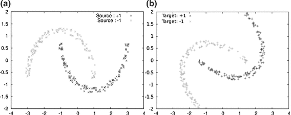
Examples from the Moons database. a Describes examples from the source domain, while b contains data from the target domain, obtained after a \(30^{\circ }\) rotation

References
Balcan M-F, Blum A (2006) On a theory of learning with similarity functions. In: Proceedings of ICML’06, pp 73–80
Balcan M-F, Blum A, Srebro N (2008) Improved guarantees for learning via similarity functions. In: Proceedings of COLT’08, pp 287–298
Bartlett PL, Mendelson S (2002) Rademacher and gaussian complexities: Risk bounds and structural results. J Mach Learn Res 3:463–482
Becker C, Christoudias C, Fua P (2013) Non-linear domain adaptation with boosting. In: Proceedings of NIPS’13, pp 485–493
Ben-David S, Blitzer J, Crammer K, Kulesza A, Pereira F, Vaughan J (2010) A theory of learning from different domains. Mach Learn 79(1–2):151–175
Bennett K, Demiriz A, Maclin R (2002) Exploiting unlabeled data in ensemble methods. In: Proceedings of KDD’02, pp 289–296
Bickel S, Brückner M, Scheffer T (2007) Discriminative learning for differing training and test distributions. In: Proceedings of ICML’07, ACM, New York, NY, USA, pp 81–88
Blitzer J, Dredze M, Pereira F (2007) Biographies, bollywood, boom-boxes and blenders: domain adaptation for sentiment classification. In: Proceedings of ACL’07
Blitzer J, McDonald R, Pereira F (2006) Domain adaptation with structural correspondence learning. In: Proceedings of EMNLP’06, pp 120–128
Blum A, Mitchell T (1998) Combining labeled and unlabeled data with co-training. In: Proceedings of the eleventh annual conference on Computational learning theory, Proceedings of COLT’98, ACM, pp 92–100
Bruzzone L, Marconcini M (2010) Domain adaptation problems: a dasvm classification technique and a circular validation strategy. IEEE Trans Pattern Anal Mach Intell 32:770–787
Chelba C, Acero A (2006) Adaptation of maximum entropy capitalizer: Little data can help a lot. Comput Speech Lang 20(4):382–399
Dai W, Yang Q, Xue G, Yu Y (2007) Boosting for transfer learning. In: Proceedings of ICML’07, pp 193–200
Daumé H III (2007) Frustratingly easy domain adaptation. In: Proceedings of ACL’07, pp 256–263
Dudík M, Schapire RE, Phillips SJ (2005) Correcting sample selection bias in maximum entropy density estimation. In: Proceedings of NIPS’05
Florian R, Hassan H, Ittycheriah A, Jing H, Kambhatla N, Luo X, Nicolov N, Roukos S (2004) A statistical model for multilingual entity detection and tracking. In: Proceedings of HLT-NAACL’04, pp 1–8
Freund Y, Schapire R (1996) Experiments with a new boosting algorithm. In: Proceedings of ICML’96, pp 148–156
Habrard A, Peyrache J-P, Sebban M (2013) Iterative self-labeling domain adaptation for linear structured image classification. Int J Artific Intell Tools 22(5). doi:10.1142/S0218213013600051
Harel M, Mannor S (2012) The perturbed variation. In: Proceedings of NIPS’12, pp 1943–1951
Huang J, Smola A, Gretton A, Borgwardt K, Schölkopf B (2006) Correcting sample selection bias by unlabeled data. In: Proceedings of NIPS’06, pp 601–608
Ji Y, Chen J, Niu G, Shang L, Dai X (2011) Transfer learning via multi-view principal component analysis. J Comput Sci Technol 26(1):81–98
Jiang J (2008) A literature survey on domain adaptation of statistical classifiers. Technical report, Computer Science Department at University of Illinois, Urbana-Champaign
Joachims T (1999) Transductive inference for text classification using support vector machines. In: Proceedings of ICML’1999, ICML ’99, pp 200–209
Kolmogorov A, Tikhomirov V (1961) \(\epsilon \)-entropy and \(\epsilon \)-capacity of sets in functional spaces. Am Math Soc Transl 2(17):277–364
Koltchinskii V (2001) Rademacher penalties and structural risk minimization. IEEE Trans Inf Theory 47(5):1902–1914
Leggetter C, Woodland P (1995) ‘Maximum likelihood linear regression for speaker adaptation of continuous density hidden markov models’. Comput Speech Lang 2:171–185
Mallapragada P, Jin R, Jain A, Liu Y (2009) Semiboost: Boosting for semi-supervised learning. IEEE T. PAMI 31(11):2000–2014
Mansour Y, Mohri M, Rostamizadeh A (2008) Domain adaptation with multiple sources. In: Proceedings of NIPS’08, pp 1041–1048
Mansour Y, Mohri M, Rostamizadeh A (2009) Domain adaptation: learning bounds and algorithms. In: Proceedings of COLT’09
Mansour Y, Schain M (2012) Robust domain adaptation. In: Proceedings of ISAIM’12
Margolis A (2011) A literature review of domain adaptation with unlabeled data, Tec. Report, pp 1–42
Martínez A (2002) Recognizing imprecisely localized, partially occluded, and expression variant faces from a single sample per class. IEEE T. PAMI 24(6):748–763
Morvant E, Habrard A, Ayache S (2011) Sparse domain adaptation in projection spaces based on good similarity functions. In: Proceedings of ICDM’11, pp 457–466
Morvant E, Habrard A, Ayache S (2012) Parsimonious unsupervised and semi-supervised domain adaptation with good similarity functions. Knowl Inform Syst (KAIS) 33(2):309–349
Pan SJ, Yang Q (2010) A survey on transfer learning. IEEE Trans Knowl Data Eng 22:1345–1359
Pérez Ó, Sánchez-Montañés MA (2007) A new learning strategy for classification problems with different training and test distributions. In: Proceedings of IWANN’07, pp 178–185
Quionero-Candela J, Sugiyama M, Schwaighofer A, Lawrence N (2009) Dataset shift in machine learning. MIT Press, Cambridge
Roark B, Bacchiani M (2003) Supervised and unsupervised pcfg adaptation to novel domains. In: Proceedings of HLT-NAACL’03
Satpal S, Sarawagi S (2007) Domain adaptation of conditional probability models via feature subsetting. In: Proceedings of PKDD’07, pp 224–235
Schapire RE, Singer Y (1999) Improved boosting algorithms using confidence-rated predictions. Mach Learn 37(3):297–336
Schapire R, Freund Y, Barlett P, Lee W (1997) Boosting the margin: A new explanation for the effectiveness of voting methods. In: Proceedings of ICML’97, pp 322–330
Sugiyama M, Nakajima S, Kashima H, von Bünau P, Kawanabe M (2008) Direct importance estimation with model selection and its application to covariate shift adaptation. In: Proceedings of NIPS’07
Tsuboi Y, Kashima H, Hido S, Bickel S, Sugiyama M (2009) Direct density ratio estimation for large-scale covariate shift adaptation, Proceedings of JIP’09 17, pp 138–155
Valiant L (1984) A theory of the learnable. Commun ACM 27(11):1134–1142
van der Vaart A, Wellner J (1996) Weak convergence and empirical processes. Springer series in statistics. Springer, Berlin
Xu H, Mannor S (2010a) Robustness and generalization. In: Proceedings of COLT’10, pp 503–515
Xu H, Mannor S (2010b) Robustness and generalization. In: Proceedings of COLT’10, pp 503–515
Xu H, Mannor S (2012a) Robustness and generalization. Mach Learn 86(3):391–423
Xu H, Mannor S (2012b) Robustness and generalization. Mach Learn 86(3):391–423
Yao Y, Doretto G (2010) Boosting for transfer learning with multiple sources. In Proceedings of CVPR’10, pp 1855–1862
Author information
Authors and Affiliations
Corresponding author
Rights and permissions
About this article

Cite this article
Habrard, A., Peyrache, JP. & Sebban, M. A new boosting algorithm for provably accurate unsupervised domain adaptation. Knowl Inf Syst 47, 45–73 (2016). https://doi.org/10.1007/s10115-015-0839-2
Received:
Revised:
Accepted:
Published:
Issue Date:
DOI: https://doi.org/10.1007/s10115-015-0839-2