
Abstract
Statistical model checking (SMC) is an analysis method that circumvents the state space explosion problem in model-based verification by combining probabilistic simulation with statistical methods that provide clear error bounds. As a simulation-based technique, it can in general only provide sound results if the underlying model is a stochastic process. In verification, however, models are very often variations of nondeterministic transition systems. In classical exhaustive model checking, partial order reduction and confluence reduction allow the removal of spurious nondeterministic choices. In this paper, we show that both can be adapted to detect and discard such choices on-the-fly during simulation, thus extending the applicability of SMC to a subclass of Markov decision processes. We prove their correctness in a uniform way and study their effectiveness and efficiency using an implementation in the modes simulator for the Modest modelling language. The examples we use highlight the different strengths and limitations of the two approaches. We find that runtime may be affected by unnecessary recomputations, and thus also investigate the feasibility of caching results to speed up simulation at the cost of increased memory usage.
1 Introduction
Traditional and probabilistic model checking have grown to be useful techniques for finding inconsistencies in designs and computing quantitative aspects of systems and protocols. However, model checking is subject to the state space explosion problem, with probabilistic model checking being particularly affected due to its additional numerical complexity. Several techniques have been introduced to stretch the limits of model checking while preserving its basic nature of performing state space exploration to obtain results that unconditionally, certainly hold for the entire state space. Two of them, partial order reduction (POR) and confluence reduction, work by selecting a subset of the transitions of a model—and thus a subset of the reachable states—in a way that ensures that the reduced system is in some sense equivalent to the complete system.
A very different approach for probabilistic models is statistical model checking (SMC) [24, 28, 41]: instead of exploring—and storing in memory—the entire state space, or even a reduced version of it, discrete-event simulation is used to generate traces through the state space. This comes at constant memory usage and thus circumvents state space explosion entirely, but cannot deliver results that hold with absolute certainty. Statistical methods such as sequential hypothesis testing are then used to make sure that the probability of returning the wrong result is below a certain threshold. As a simulation-based approach, however, SMC is limited to fully stochastic models such as Markov chains.
In this paper, we present two approaches to extend SMC and simulation to the nondeterministic model of Markov decision processes (MDP). In both, simulation proceeds as usual until a nondeterministic choice is encountered; at that point, an on-the-fly check is performed to find a singleton subset of the available transitions that satisfies either the ample set conditions of probabilistic POR [4, 12] or that is probabilistically confluent [19, 37, 38]. If such a set is found, simulation can continue that way with the guarantee that ignoring the other transitions does not affect the verification results, i.e. the nondeterminism was spurious.
The ample set conditions are based on the notion of independence of actions, which can in practice only feasibly be checked on a symbolic/syntactic level (using conditions such as J1 and J2 in [8]). This limits the approach to resolve spurious nondeterminism only when it results from the interleaving of behaviours of concurrently executing (deterministic) components.
It is absolutely vital for the search for a valid singleton subset to succeed: one choice that cannot be resolved means that the entire analysis fails and SMC cannot safely be applied to the given model at all. Therefore, any additional reduction power is highly welcome. Confluence reduction has recently been shown theoretically to be more powerful than branching time POR [19]. Furthermore, in practice, confluence reduction is easily implemented on the level of the concrete state space alone, without any need to go back to the symbolic/syntactic level for an independence check. As opposed to the POR-based approach, it thus allows even spurious nondeterminism that is internal to components to be ignored during simulation. However, confluence preserves branching-time properties and can show only nonprobabilistic (i.e. Dirac) transitions to be confluent. As we can use the less restrictive linear-time notion of POR during simulation, the two approaches are thus incomparable.
Contributions, sources and outline After the introduction of the necessary preliminaries in Sect. 2, we highlight the problems of applying SMC to nondeterministic models like MDP in Sect. 3. Two approaches to overcome these problems are to use either partial order or confluence reduction on-the-fly to detect spurious nondeterminism. They have been introduced in two conference papers before [8, 22]. In this article, we give newly formulated, general criteria for the correctness of any such reduction function-based method, in Sect. 4. This allows us to present the two approaches in a unified and uniform manner, including the correctness arguments, in Sects. 5 and 6. For the POR-based approach, this required a significant revision compared to [8] and the replacement of much of the original argumentation. For confluence, we only needed to formulate a new proof for the overall correctness (Theorem 6) that was not previously in [22]. Based on our observations when evaluating the approaches on three case studies (one from [8], extended, and two from [22]) in Sect. 7, we have built a new set of small models (Example 2) that we use from the start in this article to highlight the differences in reduction capabilities of the two approaches. Inspired by feedback we received on [22], in Sect. 8 we finally investigate the effects of caching the results of the reduction functions that were previously computed over and over again on-the-fly. These caching resolvers are a recent addition to the modes tool implementation. We conclude the article in Sect. 9.
Related work Aside from an approach that focuses on planning problems and infinite-state models [27], we are aware of three other techniques to attack the problem of nondeterminism in SMC: Henriques et al. [23] first proposed the use of reinforcement learning, a technique from artificial intelligence, to actually learn the resolutions of nondeterminism (by memoryless schedulers) that maximise probabilities for a given bounded LTL property. While this allows SMC for models with arbitrary nondeterministic choices (not only spurious ones), scheduling decisions need to be stored for every explored state. Memory usage can thus be as in traditional model checking, but is highly dependent on the structure of the model and the learning process. However, several problems in their algorithm w.r.t. to convergence and correctness have recently been described [29]. Similar learning-based methods have been picked up again by Brázdil et al. [10]. They propose two techniques that require different amounts of information about the model, but provide clear error bounds. Memory usage can again be as high as in model checking but depends on the model structure. Finally, Legay and Sedwards [29] suggest to not only sample over paths, but also over schedulers. To achieve the necessary memory efficiency, they propose an innovative O(1) encoding of a subset of all (memoryless or history-dependent) schedulers. However, their method cannot guarantee that the optimal schedulers are contained in the encodable subset and, therefore, cannot provide an error bound for the optimal probability.
Our approaches based on confluence and POR have the same theoretical memory usage bound as the learning-based ones, but use comparatively little memory in practice. They do not introduce any additional overapproximation and thus have no influence on the usual error bounds of SMC.
2 Preliminaries
We begin by giving the necessary mathematical notation and definitions from probability theory. We then define the model of Markov decision processes that we focus on in this paper, as well as a symbolic variant with variables. We finally outline the kinds of properties we want to verify, namely probabilistic reachability, and briefly summarise the available verification techniques of exhaustive and SMC.
2.1 Mathematical notation and definitions
We use angle brackets for tuples: \(\langle 2, 1 \rangle \) is a pair. We also write functions as sets \(\{\,a \mapsto b, c \mapsto d, \dots \,\}\) of mappings from the values in their domain to values in their range. \(f|_S\) denotes the restriction of function \(f\)’s domain to the set \(S\). Given an equivalence relation \(R \subseteq S \times S\) for a set \(S\), we write \([s]_R\) for the equivalence class induced by \(s\), i.e. \([s]_R = \{\, s' \in S \mid \langle s, s' \rangle \in R \,\}\). We denote the set of all such equivalence classes by \(S/R\).
Probability theory basics A (discrete) probability distribution over a countable set \(S\) is a function \(\mu \in S \rightarrow [0, 1]\) s.t. \(\sum _{s \in S}{\mu (s)} = 1\). We denote by \(\mathrm{Dist}\,\left( {S}\right) \,\) the set of all discrete probability distributions over \(S\). For \(S' \subseteq S\) and \(\mu \in \mathrm{Dist}\,\left( {S}\right) \,\), let \(\mu (S') = \sum _{s \in S'}{\mu (s)}\). We denote by \(\mathrm{support}({\mu }) = \{\,s \in S \mid \mu (s) > 0\,\}\) the support of \(\mu \). We write \(\mathcal {D}(s) \) for the Dirac distribution for \(s\), i.e. the function \(\{\,s \mapsto 1\,\}\). Given two probability distributions \(s, s' \in \mathrm{Dist}\,\left( {S}\right) \,\) and an equivalence relation \(R \subseteq S \times S\), we overload notation by writing \(\langle \mu , \mu ' \rangle \in R\) to denote that \(\mu ([s]_R) = \mu '([s]_R)\) for all \(s \in S\). For a finite set \(S = \{\,s_1, \dots , s_n\,\}\), we denote by \(\mathcal {U}(S) = \{\, s_1 \mapsto \frac{1}{n}, \dots , s_n \mapsto \frac{1}{n} \,\}\) the uniform distribution over \(S\). The product of two discrete probability distributions \(\mu _1 \in \mathrm{Dist}\,\left( {S_1}\right) \,\), \(\mu _2 \in \mathrm{Dist}\,\left( {S_2}\right) \,\) is determined by \(\mu _1 \times \mu _2(\langle s_1, s_2 \rangle ) = \mu _1(s_1) \cdot \mu _2(s_2)\).
A family \(\varSigma \) of subsets of a set \(\varOmega \) is a \(\sigma \)-algebra over \(\varOmega \) if \(\varOmega \in \varSigma \) and \(\varSigma \) is closed under complementation and countable union. A set \(B \in \varSigma \) is called measurable, and the pair \(\langle \varOmega , \varSigma \rangle \) is called a measurable space. Given a family of sets \(\mathcal {A}\), by \(\sigma (\mathcal {A})\) we denote the \(\sigma \)-algebra generated by \(\mathcal {A}\), that is the smallest \(\sigma \)-algebra containing all sets of \(\mathcal {A}\). Given a measurable space \(\langle \varOmega , \varSigma \rangle \), a function \(\mu :\varSigma \rightarrow [0,1]\) is a probability measure if \(\mu (\uplus _{i \in I}\, B_i) = \Sigma _{i \in I}\, \mu (B_i)\) for countable index sets \(I\) and \(\mu (\varOmega )=1\).
Variables and expressions When dealing with models with (discrete) variables, we need the following notions: For a set of variables \(\mathrm {Var}\) , we let \({\mathrm{Val}}({\mathrm {Var}\,})\) denote the set of variable valuations, i.e. of functions \({\mathrm {Var}\,}\rightarrow \bigcup _{x \in {\mathrm {Var}\,}} \mathrm{Dom}(x) \) where \(v \in {\mathrm{Val}}({\mathrm {Var}\,}) \Rightarrow \forall \, x \in {\mathrm {Var}\,}:v(x) \in \mathrm{Dom}(x) \). When \(\mathrm {Var}\) is clear from the context, we may write \( Val \) in place of \(\mathrm{Val}\)(\(\mathrm {Var}\) ). By \(\mathrm{Exp}\)(\(\mathrm {Var}\) ) we denote the set of expressions over the variables in \(\mathrm {Var}\) . When \(\mathrm {Var}\) is clear from the context, we may write \( Exp \) in place of \(\mathrm{Exp}\)(\(\mathrm {Var}\) ). We write \(e(v)\) for the evaluation of expression \(e\) in valuation \(v\). The set of assignments is \({\mathrm{Asgn}}({\mathrm {Var}\,}) = {\mathrm {Var}\,}\times {\mathrm{Exp}}({\mathrm {Var}\,})\), or just \( Asgn \) if \(\mathrm {Var}\) is clear from context, such that \(\langle x, e \rangle \in { Asgn \,}\Rightarrow \forall \, v \in { Val \,}:v(e) \in \mathrm{Dom}(x) \). The modification of a valuation \(v\) according to an assignment \(u\) is written as \({[\![ u ]\!]}(v)\). A set of assignments is called an update, and all the notation for assignments can be lifted to updates. We consider two restricted classes of expressions: Boolean expressions \({ Bxp \,}\subseteq { Exp \,}\) such as \(i == 1\) and arithmetic expressions \( Axp \) such as \(2.5 + x\) or \(\mathtt {ceil}(y)\).
2.2 Markov decision processes
A Markov decision process incorporates both nondeterministic and probabilistic choices on a discrete state space. Its transitions are labelled, and several transitions can be enabled in one state. The target of a transition is a probability distribution over states. Formally,
Definition 1
A Markov decision process (MDP) is a 6-tuple
where
-
\(S\) is a countable set of states,
-
\(A \supseteq \{ \tau \}\) is the alphabet, a countable set of transition labels (or actions) that includes the silent action \(\tau \),
-
\(T \in S \rightarrow \mathcal P\!\left( {A \times \mathrm{Dist}\,\left( {S}\right) \,}\right) \) is the transition function,
-
\({s_{{\mathrm {init}}}\,}\in S \) is the initial state,
-
\( AP \) is a set of atomic propositions, and
-
\(L \in S \rightarrow \mathcal P\!\left( { AP }\right) \) is the state labelling function.
Unless we say otherwise, we use the symbols from the definition above to directly refer to the components of a given MDP. We say that an MDP is finite if its set of states is finite and the transition function maps every state to a finite set of pairs \(\langle a, \mu \rangle \). We call the pairs \(\langle a, \mu \rangle \in T (s)\) the transitions of \(s\) and the triples \(\langle s, a, \mu \rangle \) such that \(\langle a, \mu \rangle \in T (s)\) the transitions of \(M\). We overload notation by writing \(\langle s, a, \mu \rangle \in T (s)\) for \(\langle a, \mu \rangle \in T (s)\) and also write \(s \mathop {\rightarrow }\limits ^{a} \mu \) for the transition \(\langle s, a, \mu \rangle \). We assume that all MDP are deadlock-free, i.e. there is at least one outgoing transition in every state.
Graphically, we represent transitions in MDP as lines with an action label that lead to an intermediate node from which the branches of the probabilistic choice lead to the respective successor states. We omit the intermediate node and probability \(1\) for transitions that lead to a Dirac distribution.
Definition 2
A transition \(\langle a, \mu \rangle \in T (s)\) for \(s \in S \) is nonprobabilistic if \(\exists \,s' :\mu = \mathcal {D}(s') \), and probabilistic otherwise. A state \(s\) is deterministic if \(|T (s)| = 1\), and nondeterministic otherwise. Likewise, an MDP is nonprobabilistic if all its transitions are nonprobabilistic, and deterministic if all its states are deterministic. A deterministic MDP is a discrete-time Markov chain (DTMC). We also write \(T (s)\) to denote the single probability distribution \(\mu \in \{\, \nu \mid \langle a, \nu \rangle \in T (s) \,\}\) in a DTMC.
An end component is a subset of the states and transitions of an MDP that is strongly connected with transition probabilities greater than \(0\):
Definition 3
An end component is a pair \(\langle S _e, T _e \rangle \) where \(S _e \subseteq S \) and \(T _e \in S _e \rightarrow \mathcal P\!\left( {A \times \mathrm{Dist}\,\left( {S}\right) \,}\right) \) with \(T _e(s) \subseteq T (s)\) for all \(s \in S _e\) such that for all \(s \in S_e\) and transitions \(\langle a, \mu \rangle \in T _e(s)\) we have \(\mu (s') > 0 \Rightarrow s' \in S _e\) and the underlying directed graph of \(\langle S _e, T _e \rangle \) is strongly connected.
As we consider closed systems only, a transition is visible if it changes the state labelling:
Definition 4
A transition \(\langle s, a, \mu \rangle \) is visible if there exists a state \(s' \in \mathrm{support}({\mu }) \) such that \(L (s) \ne L (s')\).
The semantics of an MDP is captured by the notion of paths. A path represents a concrete resolution of both nondeterministic and probabilistic choices:
Definition 5
A (finite) path in \(M\) from \(s_0\) to \(s_n\) of length \(n \in \mathbb {N} \) is a finite sequence
where \(s_i \in S \) for all \(i \in \{ 0, \dots , n \}\) and \(\langle a_i, \mu _i \rangle \in T (s_i) \wedge \mu _{i}(s_{i + 1}) > 0\) for all \(i \in \{ 0, \dots , n - 1 \}\). The set of all finite paths from the initial state \({s_{{\mathrm {init}}}\,}\) of an MDP \(M\) is denoted \(\text {Paths}_\mathrm{fin}(M)\). An (infinite) path in \(M\) starting from \(s_0\) is an infinite sequence
where for all \(i \in \mathbb {N} \), we have that \(s_i \in S \), \(\langle a_i, \mu _i \rangle \in T (s_i)\) and \(\mu _{i}(s_{i + 1}) > 0\). The set of all infinite paths starting from the initial state of an MDP \(M\) is denoted \(\text {Paths}(M)\).
Where convenient, we identify a path with the sequence of transitions \(\langle s_0, a_0, \mu _0 \rangle \, \langle s_1, a_1, \mu _1 \rangle \dots \) that it corresponds to.
In contrast to a path, a scheduler (or adversary, policy or strategy) only resolves the nondeterministic choices of an MDP. We only need memoryless schedulers in this paper, which select one outgoing transition for every state. They can be generalised to reduction functions, which select a subset of the outgoing transitions:
Definition 6
A scheduler for an MDP is a function \(\mathfrak {S} \in S \rightarrow A \times \mathrm{Dist}\,\left( {S}\right) \,\) such that \(\mathfrak {S} (s) \in T (s)\) for all \(s \in S \). A reduction function \(f \in S \rightarrow \mathcal P\!\left( {A \times \mathrm{Dist}\,\left( {S}\right) \,}\right) \) is a function such that \(f(s) \subseteq T (s)\) and \(|f(s)| > 0\) for all \(s \in S \). If \(|f(s)| = 1\) for all states, we say that \(f\) is a deterministic reduction function. The scheduler \(\mathfrak {S} \) corresponds to the deterministic reduction function \(\{\, s \mapsto \{\, \mathfrak {S} (s) \,\} \mid s \in S \,\}\). With little abuse of notation, we can thus use schedulers wherever reduction functions \(f\) are required. A scheduler \(\mathfrak {S} \) is valid for a reduction function \(f\) if \(\forall \, s \in S :\mathfrak {S} (s) \in f(s)\). The reduced MDP for \(M\) with respect to \(f\) is
where \(S _f\) is the smallest set such that
We say that \(s \in S _f\) is a reduced state if \(f(s) \ne T (s)\). All outgoing transitions of a reduced state are called nontrivial transitions. We say that a reduction function is acyclic if there are no cyclic paths in \(M_f\) starting in any state when only nontrivial transitions are considered.
As MDP allow nondeterministic choices, we can define the parallel composition of two MDP using an interleaving semantics:
Definition 7
The parallel composition of two MDP
\(i \in \{\, 1, 2 \,\}\), is the MDP \(M_1 \parallel M_2\) defined as
where
-
\(T \in (S _1 \times S _2) \rightarrow \mathcal P\!\left( {(A _1 \cup A _2) \times \mathrm{Dist}\,\left( {S _1 \times S _2}\right) \,}\right) \) s.t. \(\langle a, \mu \rangle \in T (\langle s_1, s_2 \rangle )\) if and only if \(a \notin B \wedge \exists \,\mu _1 :\langle a, \mu _1 \rangle \in T _1(s_1) \wedge \mu = \mu _1 \times \mathcal {D}(s_2) \) \(\vee \ a \notin B \wedge \exists \,\mu _2 :\langle a, \mu _2 \rangle \in T _2(s_2) \wedge \mu = \mathcal {D}(s_1) \times \mu _2\) \(\vee \ a \in B \wedge \exists \,\mu _1, \mu _2 :\langle a, \mu _1 \rangle \in T _1(s_1)\) \(\wedge \langle a, \mu _2 \rangle \in T _2(s_2) \wedge \mu = \mu _1 \times \mu _2\) with \(B = (A _1 \cap A _2) \setminus \{\, \tau \,\}\), and
-
\(L \in (S _1 \times S _2) \rightarrow \mathcal P\!\left( { AP _1 \cup AP _2}\right) \) s.t. \(L (\langle s_1, s_2 \rangle ) = L _1(s_1) \cup L _2(s_2)\).
Synchronisation in this notion of parallel composition takes place over the shared alphabet. The target of a synchronising transition is the product of the probability distributions of the individual component transitions, i.e. probabilities are multiplied. We call the parallel composition of a set of MDP a network of MDP. Parallel composition can both introduce and remove nondeterministic choices to a model.
In Sect. 5, we need to identify transitions that appear, in some way, to be the same. For this purpose, we use equivalence relations \(\equiv \) on transitions and denote the equivalence class of \({\mathrm{tr}} = \langle s, a, \mu \rangle \) under \(\equiv \) by \([{\mathrm{tr}}]_\equiv \). This notation can naturally be lifted to sets of transitions. If we are working with a network of MDP, a useful equivalence relation is the one that has \({\mathrm{tr}} \equiv {\mathrm{tr}}'\) iff the transitions \({\mathrm{tr}}\) and \({\mathrm{tr}}'\) in the product MDP result from the same set of transitions \(\{\, {\mathrm{tr}}_1, \dots , {\mathrm{tr}}_m \,\}\) in the component automata according to Definition 7. For illustration, consider the network of MDP \(\{\, M_1, M_2, M_3 \,\}\) shown in Fig. 1. The product MDP on the right has two equivalence classes of transitions, as shown below the MDP in the figure: The transitions labelled a are in the same class because they both result from the synchronisation of \(\langle 0, \mathtt{a }, \mathcal {D}(1) \rangle \) from \(M_1\) and \(\langle 2, \mathtt{a }, \mathcal {D}(3) \rangle \) from \(M_2\). The two transitions labelled \(\tau \) belong to the same class because they both result from transition \(\langle 4, \tau , \mathcal {D}(5) \rangle \) of \(M_3\).

Transition equivalence \(\equiv \) illustrated
2.3 MDP with variables
Building MDP models becomes easier when we allow the inclusion of variables. In the resulting model of Markov decision processes with variables (VMDP), variables can be read in guards and changed in updates. The target of an edge is a symbolic probability distribution.
Definition 8
A VMDP is a 7-tuple
where
-
\(\mathrm {Loc}\) is a countable set of locations,
-
\(\mathrm {Var}\) is a finite set of variables with countable domains,
-
\(A \supseteq \{ \tau \}\) is the alphabet,
-
\(E \in \mathrm {Loc} \rightarrow \mathcal P\!\left( {{ Bxp \,}\times A \times (\mathcal P\!\left( {{ Asgn \,}}\right) \times \mathrm {Loc} \rightarrow { Axp \,})}\right) \) is the edge function, which maps each location to a set of edges, which in turn consist of a guard, a label and a symbolic probability distribution that assigns weights to pairs of updates and target locations,
-
\({l_{\mathrm {init}}\,}\in \mathrm {Loc} \) is the initial location,
-
\({V_{\mathrm {init}}\,}\in {\mathrm{Val}}({\mathrm {Var}\,})\) is the initial valuation of the variables, and
-
\({ VExp \,}\subseteq { Bxp \,}\) is the set of visible expressions.
Unless we say otherwise, we use the symbols from the definition above to directly refer to the components of a given VMDP. We also write \(l \mathop {\rightarrow }\limits ^{g, a} m\) instead of \(\langle g, a, m \rangle \in E (l)\). As for MDP, we may refer to an edge as \(\langle l, g, a, m \rangle \) if \(\langle g, a, m \rangle \in E (l)\).
The semantics of a VMDP is an MDP whose states keep track of the current location and the current values of all variables. Based on these values, the symbolic probability distributions can be turned into concrete ones as follows: let \(m \in (\mathcal P\!\left( {{ Asgn \,}}\right) \times \mathrm {Loc}) \rightarrow { Axp \,}\). We require that it evaluates to a non-zero expression only on a countable range \(R \subset \mathcal P\!\left( {{ Asgn \,}}\right) \times \mathrm {Loc} \). The corresponding concrete probability distribution is determined as
for valuations \(v\) for the variables of the VMDP. For any reachable valuation \(v\), we need that \(m(\langle U, l \rangle )(v) \ge 0\) for all \(\langle U, l \rangle \in R\) and \(\sum _{\langle U, l \rangle \in R}{m(\langle U, l \rangle )}(v)\) converges to a positive real value. We consider it a modelling error if this is not the case.
Definition 9
The semantics of a VMDP is the MDP
where
-
\(T \in \mathrm {Loc} \times { Val \,}\rightarrow \mathcal P\!\left( {A \times \mathrm{Dist}\,\left( {\mathrm {Loc} \times { Val \,}}\right) \,}\right) \) such that \(\langle a, \mu \rangle \in T (\langle l, v \rangle )\) if and only if
$$\begin{aligned}&\exists \,\langle g, a, m \rangle \in E (l) :g(v) \wedge \mu = m_{\mathrm{conc}}^v\nonumber \\ \vee \,&a = \tau \wedge \mu = \mathcal {D}(l) \wedge \not \exists \,\langle g, a, m \rangle \in E (l) :g(v) \end{aligned}$$(1)and
-
\(L \in (\mathrm {Loc} \times { Val \,}) \rightarrow \mathcal P\!\left( {{ VExp \,}}\right) \) such that \(\forall \langle l, v \rangle \in \mathrm {Loc} \times { Val \,}:L (\langle l, v \rangle ) = \{\, e \in { VExp \,}\mid e(v)\, \}\).
Observe that the second line of Eq. (1) adds a loop to a state in the MDP in case no edge is enabled. This explicitly ensures that the result is deadlock-free.
In the parallel composition of VMDP, the symbolic probability distributions are combined by simply creating multiplication expressions:
Definition 10
The parallel composition of two consistent VMDP \(M_i = \langle \mathrm {Loc} _i, {\mathrm {Var}\,}_i, A _i, E _i, {l_{\mathrm {init}}\,}_{i}, {V_{\mathrm {init}}\,}_i, { VExp \,}_i \rangle \), \(i \in \{1, 2\}\), is the VMDP \(M_1 \parallel M_2\) defined as
where \(E \in (\mathrm {Loc} _1 \times \mathrm {Loc} _2) \rightarrow \mathcal P\!\left( {{ Bxp \,}\times A _1 \cup A _2 \times {SPr}}\right) \) with \({SPr} = (\mathcal P\!\left( {{ Asgn \,}}\right) \times (\mathrm {Loc} _1 \times \mathrm {Loc} _2) \rightarrow { Axp \,})\) s.t. \(\langle g, a, m \rangle \in E (\langle l_1, l_2 \rangle )\) if and only if
where \(B = (A _1 \cap A _2) \setminus \{ \tau \}\) and the product of two consistent symbolic probability distributions \(m_i\), \(i \in \{\, 1, 2 \,\}\), is defined as
We allow shared variables. This is why we need the two components to be consistent. Consistency means that the initial valuations agree on the shared variables and that there are no conflicting assignments.
As for MDP parallel composition, a useful equivalence relation \(\equiv \) over the transitions of the MDP semantics of a network of VMDP is the one that identifies those transitions that result from the same (set of) edges in the component VMDP. We denote this relation by \(\equiv _E \).
2.4 Probabilistic reachability
In this paper, we consider the verification of probabilistic reachability properties. Syntactically, we can write such a property as \({P}_{\max }(\diamond \,\phi )\) and \({P}_{\min }(\diamond \,\phi )\). Intuitively, they represent a query for the maximum or minimum probability of reaching a state whose labelling satisfies the state formula \(\phi \) (a \(\phi \)-state for short) from the initial state of an MDP. A state formula can represent undesirable configurations of the system (or “bad” states); in that case, we typically want to check whether the maximum probability of reaching such a state is sufficiently low. If, on the other hand, it represents desirable configurations that should be reached in a correct or reliable system, then we would like to ensure that the minimum probability of reaching any of them is high.
The actual probability of reaching a certain set of states depends on how the nondeterministic choices of an MDP are resolved, i.e. on which scheduler is used. When ranging over all possible schedulers, we obtain an interval \(\subseteq [0, 1]\) of possible probabilities. As we could see in the examples above, for verification, it is the interval’s extremal values that we are interested in, i.e. the minimum and maximum probabilities. Formally, the semantics is defined as followsFootnote 1:
Definition 11
The semantics of a probabilistic reachability query \({P}_{\max }(\diamond \,\phi )\) or \({P}_{\min }(\diamond \,\phi )\) is defined as
As usual, we omit the subscript \(M\) when it is clear from the context. Observe that the \(\mathrm{red}(M, \mathfrak {S})\) are DTMC. A proof of the facts that 1) a scheduler exists that maximises/minimises the reachability probability and that 2) this scheduler is memoryless can be found in, for example, [5] as the proof of lemmas 10.102 and 10.113.
In the definition above, we have only dealt with the nondeterministic choices. In order to define the meaning of \({[\![ {P}(\diamond \,\phi ) ]\!]}_M\) for a DTMC \(M\), we assign probabilities to the (finite) paths that lead to \(\phi \)-states from the initial state. We need the construct of cylinder sets cylinder set to properly define a probability measure on finite paths.
Definition 12
The cylinder set of a finite path \(\hat{\pi }\!\in \! \text {Paths}_\mathrm{fin}(M)\) for a DTMC \(M\) is defined as
Now let \(\mathrm{Cyl}(M) \mathop {=}\limits ^{\mathrm{ def}}\{\, \mathrm{Cyl}(\hat{\pi }) \mid \hat{\pi }\in \text {Paths}_\mathrm{fin}(M) \,\}\) denote the set of all cylinder sets of \(M\). Then the pair \(\langle \mathrm{Cyl}(M), \sigma (\mathrm{Cyl}(M)) \rangle \) is a measurable space. This allows us to define a probability measure \(\mathrm{Prob}_M\) for \(M\) by assigning probabilities to cylinder sets as follows:
Definition 13
For a DTMC \(M\), \(\mathrm{Prob}_M\) is the probability measure on the \(\sigma \)-algebra \(\langle \mathrm{Cyl}(M), \sigma (\mathrm{Cyl}(M)) \rangle \) uniquely determined by
where \(s_0 = {s_{{\mathrm {init}}}\,}\) by definition.
We can informally say that \(\mathrm{Prob}_M\) assigns probabilities to finite paths, which is what is needed to finally define the semantics of a probabilistic reachability query on DTMC resp. deterministic MDP:
Definition 14
The semantics of \({P}(\diamond \,\phi )\) on a DTMC \(M\) is
where
is the set of finite paths on which the last state is the only one whose labelling satisfies \(\phi \).
Since the set \(\text {Paths}_\mathrm{fin}(\phi , M)\) is countable, the union of the corresponding cylinder sets is a countable union and thus measurable. \({[\![ {P}(\diamond \,\phi ) ]\!]}_M\) is, therefore, well defined. The probability of the union is equal to the sum of the probabilities of the individual cylinder sets because they are pairwise disjoint by the definition of \(\text {Paths}_\mathrm{fin}(\phi , M)\).
Temporal logics
More complex properties for MDP can be specified using temporal logics such as PCTL* or probabilistic LTL. What is important for this paper, in particular for the correctness of the techniques presented in Sects. 5 and 6, is that probabilistic reachability can be expressed in probabilistic LTL as well as in PCTL*.
2.5 Computing reachability probabilities
Several techniques are available to implement the computation of actual values \({[\![ {P}_{\max }(\diamond \,\phi ) ]\!]}_M\) of probabilistic reachability properties.
2.5.1 Exhaustive model checking
The classic approach in verification is to perform exhaustive model checking: First, all reachable states in the MDP are collected and stored, and the \(\phi \)-states are identified. Then, a numeric algorithm is used to obtain the probability of reaching those states from the initial one. Examples of such algorithms are solving a linear programming problem, value iteration, and policy iteration [5, 14]. The results of exhaustive model checking are exact, or can at least be made arbitrarily close to the true probabilities. However, it is only applicable to finite MDP and suffers from the state-space explosion problem: every new variable in a model results in a worst-case exponential growth of the number of states, which need to be represented in some form in limited computer memory. Detailed models of real-world systems quickly grow too large for exhaustive model checking.
2.5.2 Statistical model checking
An alternative to exhaustive model checking for the fully stochastic model of DTMC is statistical model checking (SMC [24, 28, 41]). The idea is to randomly generate a number of paths, determine for each whether the relevant set of states is reached, and then use statistical methods to derive an approximation of the reachability probability. This approximation is usually associated with some level of confidence or specific error bounds guaranteed by the particular statistical method used. We refer to the path generation step as simulation of the DTMC, and refer by SMC to the complete procedure including the statistical analysis. SMC comes at constant memory usage and thus circumvents state-space explosion entirely, but cannot deliver results that hold with absolute certainty. Algorithm 1 shows a simulation procedure for DTMC. It takes as parameters the DTMC \(M\), state formula of interest \(\phi \) and maximum path length \(d\).

Finite paths for unbounded reachability As we are interested in probabilistic reachability properties, we need to explore paths in a way that allows us to determine whether a \(\phi \)-state is eventually reached or not. In particular, it does not suffice to give up and return \( unknown \) in all cases where no \(\phi \)-state is seen up to a certain path length. Algorithm 1 shows a practical solution to this problem: It keeps track of the states visited since the last non-Dirac choice; when we return to such a state, we have discovered a (probability 1) cycle. When this happens, we can conclude that the current path will never reach a \(\phi \)-state. To ensure termination for models whose non-\(\phi \)-paths do not all end in a Dirac cycle, we still include a maximum path length parameter \(d\). This complication results from the fact that we verify unbounded reachability properties, yet we can only explore finite prefixes of paths.
Sample mean and confidence Every run of the function simulate under these conditions (assuming it never aborts with \( unknown \)) explores a finite path \(\hat{\pi }\) and returns \( true \) if \(\hat{\pi }\in \text {Paths}_\mathrm{fin}(\phi , M)\), otherwise \( false \) (which in particular means that no path in \(\mathrm{Cyl}(\hat{\pi }) \) contains a \(\phi \)-state). Since the probability distributions used in line 9 of Algorithm 1 are exactly those given by the model, the probability of encountering any one of these paths in a single run is \(\mathrm{Prob}_M(\mathrm{Cyl}(\hat{\pi }))\). We let the random variable \(X\) be the result of a simulation run. If we interpret \( true \) as \(1\) and \( false \) as \(0\), then \(X\) follows the Bernoulli distribution with success parameter, and hence expected value, of \({[\![ {P}(\diamond \,\phi ) ]\!]}\). This is the foundation for the statistical evaluation of simulation data [35, Chapter 7]: a batch of \(k\) simulation runs corresponds to \(k\) random variables that are independent and identically distributed with expected value \(p = {[\![ {P}(\diamond \,\phi ) ]\!]}\). The average \(\overline{X} = \sum _{i=1}^k{X_i/k}\) of the \(k\) random variables, the sample mean, is then an approximation of \(p\). (It is in fact an unbiased estimator of that actual mean.)
The single quantity of sample mean, however, is fairly useless for verification. We also need to know how good an approximation of \(p\) it is. They key parameter to influence the quality of approximation is \(k\), the number of simulation runs performed. The higher \(k\) is, the more confident can we be that a concrete observed sampled mean \(\overline{x}\) is close to \(p\). There are various statistical methods to precisely describe this notion of confidence and determine the actual confidence for a given set of simulation results. A widely used method is to compute a confidence interval confidence interval [35] of width \(2\epsilon \) around \(\overline{x}\) with confidence level \(100 \cdot (1 - \alpha )\). Typically, \(k\) and \(\alpha \) are specified by the user and \(\epsilon \) is then derived from \(\alpha \) and the collected observations of the \(X_i\). Confidence intervals are not without problems [1], so we explain the alternative APMC method in more detail below. This is to provide a complete context; the techniques we present later in this paper do not depend on the concrete statistical method used.

The APMC method The approximate probabilistic model checking (APMC) method was introduced with and originally implemented in a tool of the same name [24]. The key idea is to use Chernoff–Hoeffding bounds [25] to relate the three parameters of approximation \(\epsilon \), confidence level \(\delta \), and number of simulation runs \(k\) in such a way that we have
i.e. the difference between computed and actual probability is at most \(\epsilon \) with probability \(1 - \delta \). There are several ways to relate the three values. The Prism tool [31], for example, uses the formula

Algorithm 2, based on [24] and [31], combines this relationship and the simulate function of Algorithm 1 to implement a complete SMC procedure using the APMC method.
3 SMC versus nondeterminism in MDP
Using SMC to analyse probabilistic reachability properties on MDP models is problematic: In order to generate a path through an MDP, we not only have to conduct a probabilistic experiment in each state, but also resolve the nondeterminism between the outgoing transitions first. These latter scheduling choices determine which probability out of the interval between maximum and minimum we actually observe in SMC. As the only relevant values in verification are the actual maximum and minimum probabilities, we would need to be able to use the corresponding extremal schedulers to obtain useful results. These schedulers are not known in advance, however.
3.1 Resolving nondeterminism
Extending the DTMC simulation technique of Algorithm 1 to MDP by also resolving the nondeterministic choices results in Algorithm 3. The only addition is line 7. It takes as an additional parameter a resolver \(\mathfrak {R}\), i.e. a function in \(S \rightarrow \mathrm{Dist}\,\left( {A \times \mathrm{Dist}\,\left( {S}\right) \,}\right) \,\) s.t.
for all states \(s\). If we burden the user with the task of specifying \(\mathfrak {R}\), SMC for MDP is easy as this would immediately allow the function simulate of Algorithm 3 to be used for path generation in existing SMC algorithms for DTMC.

Many simulation tools, including e.g. the simulation engine that is part of the Prism probabilistic model checker [26], in fact implicitly use a specific built-in resolver so users do not even need to bother specifying one. On the other hand, this means that users are not able to do so if they wanted to, either. The implicit resolver that is typically used makes a uniformly distributed choice between the available transitions:
However, one can think of other generic resolvers. For example, a total order on the actions (i.e. priorities) can be specified by the user, with the corresponding resolver making a uniform choice only between the available transitions with the highest-priority label. A special case of this appears when we consider MDP that model the passage of a unit of physical time with a dedicated tick action: if we assign the lowest priority to tick, we schedule the other transitions as soon as possible; if we assign the highest priority to tick, we schedule the other transitions as late as possible.
Unfortunately, just performing SMC with some implicit scheduler as described above is not sound: while a probabilistic reachability property asks for the minimum or maximum probability of reaching a set of target states, using an implicit scheduler merely results in some probability in the interval between minimum and maximum.
Definition 15
An SMC procedure for MDP is sound if, given any MDP \(M\) and property \({P}_{\max }(\diamond \,\phi )\) or \({P}_{\min }(\diamond \,\phi )\), it returns a sample mean \(p_{\mathrm{smc}}\) and a useful confidence statement relating \(p_{\mathrm{smc}}\) to \({[\![ {P}_{\max }(\diamond \,\phi ) ]\!]}\) or \({[\![ {P}_{\min }(\diamond \,\phi ) ]\!]}\), respectively.
Observe that we informally require a “useful” confidence statement. This is in order to remain abstract w.r.t. the concrete statistical method used. We consider e.g. confidence intervals with small \(\epsilon \) and \(\alpha \) or an APMC confidence \(\langle k, \epsilon , \delta \rangle \) with small \(\epsilon \) and \(\delta \) useful. In contrast, merely reporting some probability between minimum and maximum means that the potential error can be arbitrarily close to \(1\). This may still be of use in some applications, but is not a useful statement for verification.
Example 1
Figure 2 shows a nonprobabilistic MDP that models a discrete-timed system with a special tick action as described above. It contains two nondeterministic choices between the action go and letting time pass. Let the property of interest be one of performance, namely whether a state labelled with atomic proposition final can be reached with probability at least \(0.5\) in time at most \(t\), i.e. by taking at most \(t\) transitions labelled tick. When we encode that number in the atomic propositions as well, we need to check for \(i \in \{0, \dots , 100\}\) whether \({[\![ {P}_{\max }(\diamond \, \text {final} \wedge i) ]\!]} \ge 0.5\). The maximum and minimum \(i\) for which this is true are then the maximum and minimum time needed to reach a final state with probability \(\ge 0.5\).

An anomalous discrete-timed system
The results we would obtain via exhaustive model-checking are a minimum (best-case) time of \(2\) ticks and a maximum (worst-case) time of \(100\) ticks. For an SMC analysis, the nondeterminism needs to be resolved. Using \(\mathfrak {R}_\mathrm{Uni}\), the result would be around \(27\) ticks. Note that this is quite far from the actual worst-case behaviour. In particular, by adding more “fast” or “slow” alternatives to the model, we can arbitrarily change the SMC result. Even worse, a very small change to the model can make quite a big difference: If the go-labelled transition to the upper branch were available in the initial state instead of after one tick, the “uniform” result would be \(35\) ticks.
Knowing that this is a timed model, we could try the ASAP and ALAP resolvers. Intuitively, we might expect to obtain the best-case behaviour for ASAP and the worst-case behaviour for ALAP. Unfortunately, the results run counter to this intuition: ASAP yields a time of \(3\) ticks, ALAP leads to the best-case result of \(2\) ticks, and the worst case of \(100\) ticks is completely ignored. This is because the example exhibits a timing anomaly: it is best to wait as long as possible before taking go to obtain the minimum time. For this toy example, the anomaly can easily be seen by looking at the model, but similar effects (not limited to timing-related properties) may of course occur in complex models where they cannot so easily be spotted.
While problems with the credibility of simulation results have been observed before [2], most state-of-the-art simulation and SMC tools still implicitly resolve nondeterminism, typically using \(\mathfrak {R}_\mathrm{Uni}\). We argue that using some resolution method under-the-hood in an SMC tool—without warning the user of the possible consequences—is dangerous. As a consequence, our modes tool that provides SMC within the Modest Toolset (cf. Sect. 7) in its default configuration aborts with an error when a nondeterministic choice is encountered. While it is possible to select between different built-in resolvers to have modes simulate such models anyway, including \(\mathfrak {R}_\mathrm{Uni}\), this requires deliberate action on part of the user.
4 Spuriously nondeterministic MDP
The two approaches to perform SMC for MDP in a sound way we present in this paper exploit the fact that resolving a nondeterministic choice in one way or another does not necessarily make a difference for the property at hand. In such a case, the choice is spurious, and any resolution leads to the same probability. When all nondeterministic choices in an MDP are spurious for some reachability property, then the maximum and minimum probability coincide and SMC results can be relied upon. Consider the following example:
Example 2
Communication protocols often have to transfer messages in a broadcast fashion over shared media where a collision results if two senders transmit at the same time. In such an event, receivers are unable to extract any useful data out of the ensuing distortion. In Fig. 3, we show VMDP modelling the sending of a message in such a scenario.Footnote 2 Processes \(H_i^a\) represent the senders, or hosts, which communicate with two alternative models \(M_\mathrm{var}\) and \(M_\mathrm{sync}\) for the shared medium that observes whether a message is transmitted successfully or a collision occurs. Communication with \(M_\mathrm{var}\) is by synchronisation on tick and via shared variable \(i\), while communication with \(M_\mathrm{sync}\) is purely by synchronisation. The full models we are interested in are the networks \(N_v^a = \{\, H_1^a, H_2^a, M_v \,\}\) for all four combinations of \(a \in \{\,\mathtt{a }, \tau \,\}\) and \(v \in \{\,\mathrm{var}, \mathrm{sync}\,\}\).
Seen on their own, the host VMDP as well as their MDP semantics are deterministic. \(M_\mathrm{var}\) looks nondeterministic as a VMDP but its semantics is a deterministic MDP, while \(M_\mathrm{sync}\) and its semantics are nondeterministic. If we consider the MDP semantics of the networks, we can with moderate effort see that they all contain at least one nondeterministic state, namely when both hosts happen to be in location \(h_2\), and possibly more. Still, we have that \({P}_{\min }(\diamond \,\mathrm{success}) = {P}_{\max }(\diamond \,\mathrm{success}) = 0.5\) and \({P}_{\min }(\diamond \,\mathrm{collide}) = {P}_{\max }(\diamond \,\mathrm{collide}) = 0.25\). For the given atomic propositions, all the nondeterministic choices are thus spurious. As for the problem highlighted by Fig. 2 previously, this is relatively easy to see for these small models, but will usually be anything but obvious for larger, more complex, and realistic networks of MDP.
4.1 Reduced deterministic MDP
In order to perform SMC for spuriously nondeterministic MDP as those presented in the previous example, it suffices to supply a resolver to the path generation procedure of Algorithm 3 that corresponds to a deterministic reduction function and that preserves minimum and maximum reachability probabilities. Formally, we want to use a reduction function \(f\) such that
The existence of such a reduction function for a given MDP and property indeed means that the minimum and the maximum probability are the same:
Proposition 1
Given an MDP \(M\) and a state formula \(\phi \) over its atomic propositions, we have that
Proof
Because \(f\) is deterministic, \(\mathrm{red}(M, f)\) is deterministic (i.e. a DTMC). Therefore, we have
and it follows by Eq. (3) that
\(\square \)
The existence of a reduction function satisfying Eq. (3) consequently means that all nondeterministic choices in the MDP can be resolved in such a way that SMC computes the actual minimum and maximum probability (which are necessarily the same). Moreover, it means that no matter how we resolve the nondeterminism, we obtain the correct probabilities:
Theorem 1
Given an MDP \(M\) and a state formula \(\phi \) over its atomic propositions, we have that
Proof
By contraposition and contradiction using Proposition 1.
We could also show the same result for resolvers instead of reduction functions. This means that we could use \(\mathfrak {R}_\mathrm{Uni}\) and obtain correct results, too—that is, if we know that a reduction function satisfying Eq. (3) exists for the given model and property. Unfortunately, attempting to find such a function for all states at once, before we start simulation, would negate the core advantage of SMC over exhaustive model checking: its constant or low memory usage.
4.2 Preservation of probabilistic reachability
The reduction functions we are looking for need to satisfy two relatively separate requirements according to Eq. (3): they need to be deterministic, and they need to preserve maximum and minimum reachability probabilities. The former is a simple property that appears easy to check or ensure by construction. However, it is not so obvious what kind of criteria would guarantee the latter.
In exhaustive model checking, equivalence relations that divide the state space into partitions of states with “equivalent” behaviour have been studied extensively: they allow the replacement of large state spaces with smaller quotients under such a relation and thus help alleviate the state-space explosion problem. We aim to build upon this research to construct our reduction functions. As we are interested in the verification of probabilistic reachability properties, we could potentially use any equivalence relation that preserves those properties:
Definition 16
An equivalence relation \(\sim \) over MDP preserves probabilistic reachability if, for all pairs \(\langle M_1, M_2 \rangle \) of MDP with the same atomic propositions, we have that
and also
Candidates for \(\sim \) would be appropriate variants of trace equivalence, simulation or bisimulation relations. In fact, it turns out that there are two well-known techniques to reduce the size of MDP in exhaustive model checking that appear promising: partial order reduction [3, 16, 33, 39] and confluence reduction [7, 37, 38]. Both provide an algorithm to obtain a reduction function such that the original and the reduced model are equivalent according to relations that preserve probabilistic reachability. Both algorithms can be performed on-the-fly while exploring the state space [17, 34], which avoids having to store the entire (and possibly too large) state space in memory at any time. Instead, the reduced model is generated directly. We, therefore, study in Sects. 5 and 6 whether the two algorithms can be adapted to compute a reduction function on-the-fly during simulation with little extra memory usage.
4.3 Partial exploration during simulation
If we compute the reduction function on-the-fly, however, we only compute it for a subset of the reachable states, namely those visited during the simulation runs of the current SMC analysis. We are thus unable to check whether the supposedly simple first requirement of Eq. (3), determinism, actually holds for all states of the model, or at least (and sufficiently) for all states in the reduced state space.
Yet, requiring determinism for all states is more restrictive than necessary. Instead of Eq. (3), let us require that the reduction function \(f\) computed on-the-fly during the calls to function simulate in one concrete SMC analysis satisfies
where \(T \) is the transition function of \(M\) and \(\varPi \) is the set of paths explored during the simulation runs and we abuse notation to write \(s \in \varPi \) in place of \(s \in \{\,s' \in S \mid \exists \, \ldots s' \ldots \in \varPi \,\}\). This means that the function still has to preserve probabilistic reachability, and it still must be deterministic on the states we visit during simulation, but on all other states, it is now required to perform no reduction instead. As before, if we compute \(f\) such that \(M \sim \mathrm{red}(M, f)\) is guaranteed for a relation \(\sim \) that preserves probabilistic reachability, we already know that the last two lines of Eq. (4) are satisfied.
Although Proposition 1 and Theorem 1 do not hold for such a reduction function in general, let us now show why it still leads to a sound SMC analysis in the sense of Definition 15. Recall that, for every MDP \(M\) and state formula \(\phi \), there are schedulers \(\mathfrak {S} _{\max }\) and \(\mathfrak {S} _{\min }\) that maximise resp. minimise the probability of reaching a \(\phi \)-state, i.e.
If \(f\) is a reduction function that satisfies Eq. (4), then there is at least one such maximising (minimising) scheduler \(\mathfrak {S} _{\max }\) (\(\mathfrak {S} _{\min }\)) that is valid for \(f\). For the states where \(f\) is deterministic, this is the case due to the third (fourth) line of Eq. (4). For this scheduler, we, therefore, also have
(and the corresponding statement for \(\mathfrak {S} _{\min }\)). When exploring the set of paths \(\varPi \), by following \(f\), the simulation runs also followed both \(\mathfrak {S} _{\max }\) and \(\mathfrak {S} _{\min }\) (due to determinism of \(f\) on \(\varPi \) and the schedulers being valid for \(f\)). The resulting sample mean is thus the same as if we had performed the simulation runs on either of the DTMC \(\mathrm{red}(M, \mathfrak {S} _{\max })\) or \(\mathrm{red}(M, \mathfrak {S} _{\min })\). In consequence, whatever statement connecting the sample mean and the actual result we obtain from the ensuing statistical analysis is correct. In particular, we do not need to modify the reported confidence to account for nondeterministic choices that we did not encounter on the paths in \(\varPi \): We already did simulate the correct “maximal”/“minimal” DTMC.
We can now adapt the simulation function given in Algorithm 3 to use a procedure \(\mathfrak {A}\) instead of a resolver \(\mathfrak {R}\). \(\mathfrak {A}\) acts as a function \(S \rightarrow (A \times \mathrm{Dist}\,\left( {S}\right) \,) \cup \{\,\bot \,\}\) and on-the-fly computes the output of a reduction function satisfying Eq. (4). It returns a transition to follow during simulation if the current state is deterministic or if it can show the nondeterminism to be spurious. Otherwise, it returns \(\bot \), which causes both the current simulation run as well as the SMC analysis to be aborted. In particular, for the underlying reduction function \(f\) to satisfy Eq. (4), \(\mathfrak {A}\) must be implemented in a deterministic manner, i.e. it must always return the same transition for the same state. When the SMC analysis terminates successfully (i.e. \(\mathfrak {A}\) has never returned \(\bot \)), \(\mathfrak {A}\) will have determined \(f\) to singleton sets for the states visited, and we complete \(f\) to map all other states \(s\) to \(T (s)\) for the correctness argument.
It now remains to find out whether there are such procedures \(\mathfrak {A}\) that are both efficient (i.e. they do not destroy the advantage of SMC in memory usage and they do not excessively increase runtime) and effective (i.e. they never return \(\bot \) for some practically relevant models). It turns out that at least a check inspired by partial order reduction techniques, which we present in Sect. 5, and checking for confluent transitions as we show in Sect. 6, work well. We investigate the efficiency and effectiveness of the two approaches using three case studies in Sect. 7.
5 Using partial order reduction
For exhaustive model checking of networks of VLTS, an efficient method already exists to deal with models containing spurious nondeterminism resulting from the interleaving of parallel processes: partial order reduction (POR, [16, 33, 39]). It reduces such models to smaller ones containing only those paths of the interleavings necessary to not affect the end result. POR was first generalised to the probabilistic domain preserving linear time properties, including probabilistic LTL formulas without the next operator X [4, 12], with a later extension to preserve branching time properties without next, i.e. \(\text {PCTL*}_{\setminus \text {X}}\) [3]. In the remainder of this section, we first recall how POR for MDP works and then detail how to harvest it to compute a reduction function satisfying Eq. (4) on-the-fly during simulation. The relation \(\sim \) between the original and the reduced model guaranteed by this approach is stutter equivalence, which preserves the probabilities of \(\text {LTL}_{\setminus \text {X}}\) properties [3].Footnote 3
5.1 Partial order reduction for MDP
The aim of partial order techniques for exhaustive model checking is to avoid building the full state space corresponding to a model. Instead, a smaller state space is constructed and analysed where the spurious nondeterministic choices resulting from the interleaving of independent transitions are resolved. The reduced system is not necessarily deterministic, but smaller, which increases the performance and reduces the memory demands of exhaustive model checking (if the reduction procedure is less expensive than analysing the full model right away).
Partial order reduction has first been generalised to the MDP setting [3] based on the ample set method [33] for nonprobabilistic systems. A probabilistic extension of stubborn sets [39] has been developed later, too [18]. Our approach is based on ample sets. The essence is to identify an ample set of transitions \(\mathsf {ample}(s)\) for every state \(s \in S \) of the MDP \(M\), yielding the reduction function
such that conditions A0–A4 of Table 1 are satisfied (where \(S _f\) denotes the state space of \(M_f = \mathrm{red}(M, f)\), cf. Definition 6).
For partial order reduction, the notion of (in)dependent transitionsFootnote 4 (rule A2) is crucial. Intuitively, the order in which two independent transitions are executed is irrelevant in the sense that they do not disable each other (forward stability) and that executing them in a different order from a given state still leads to the same states with the same probabilities (commutativity). Formally,
Definition 17
Two equivalence classes \([{\mathrm{tr}}'_1]_\equiv \ne [{\mathrm{tr}}'_2]_\equiv \) of transitions of an MDP are independent iff for all states \(s \in S \) with \({\mathrm{tr}}_1, {\mathrm{tr}}_2 \in T (s)\), \({\mathrm{tr}}_1 = \langle s, a_1, \mu _1 \rangle \in [{\mathrm{tr}}'_1]_\equiv \), \({\mathrm{tr}}_2 = \langle s, a_2, \mu _2 \rangle \in [{\mathrm{tr}}_2']_\equiv \),
- I1:
-
\(s' \in \mathrm{support}({\mu _1}) \Rightarrow {\mathrm{tr}}_2 \in [T (s')]_\equiv \) and vice-versa (forward stability), and then also
- I2:
-
\(\sum _{s'' \in S}{\mu _1(s'') \cdot \mu _2^{s''}(s')} = \sum _{s'' \in S}{\mu _2(s'') \cdot \mu _1^{s''}(s')}\) for all \(s' \in S \) (commutativity),
where \(\mu _i^{s''}\) is the single element of \(\{\, \mu \ |\ \langle s'', a_i, \mu \rangle \in T (s'') \cap [{\mathrm{tr}}_i]_\equiv \,\}\).
Checking dependence by testing these conditions on all pairs of transitions for all states of an MDP is impractical. Partial order reduction is thus typically applied to the MDP semantics of networks of VMDP where sufficient and easy-to-check conditions on the symbolic level can be used. In that setting, \(\equiv _E \) is used for the equivalence relation \(\equiv \). Then, two transitions \({\mathrm{tr}}_1\) and \({\mathrm{tr}}_2\) in the MDP correspond to two edges \(e_i = \langle l_i, g_i, a_i, m_i \rangle \) on the level of the parallel composition semantics of the network of VMDP. Each of these edges in turn is the result of one or more individual edges in the component VMDP. We can thus associate with each transition \({\mathrm{tr}}_i\) a (possibly synchronised) edge \(e_i\) and a (possibly singleton) set of component VMDP. The following are then an example of such sufficient and easy-to-check symbolic-level conditions:
- J1:
-
The sets of VMDP that \({\mathrm{tr}}_1\) and \({\mathrm{tr}}_2\) originate from are disjoint, and
- J2:
-
for all valuations \(v\),
$$\begin{aligned}&~m_1(\langle U_1, l' \rangle ) \ne 0 \wedge m_2(\langle U_2, l' \rangle ) \ne 0\\&\Rightarrow \begin{aligned}&(g_2(v) \Rightarrow g_2({[\![ A_1 ]\!]}(v)))\\&\!\wedge {[\![ A_1 ]\!]}({[\![ A_2 ]\!]}(v)) = {[\![ A_2 ]\!]}({[\![ A_1 ]\!]}(v)) \end{aligned} \end{aligned}$$and vice-versa.
J1 ensures that the only way for the two transitions to influence each other is via global variables, and J2 makes sure that this does not actually happen, i.e. each transition modifies variables only in ways that do not disable the other’s guard and the assignments are commutative. This check can be implemented on a syntactic level for the guards and the expressions occurring in assignments.
Using the ample set method with conditions A0–A4 and I1–I2 or J1–J2 gives the following result:
Theorem 2
[3] If an MDP \(M\) is reduced to an MDP \(\mathrm{red}(M, f_\mathsf {ample})\) using the ample set method as described above, then \(M \sim \mathrm{red}(M, f_\mathsf {ample})\) where \(\sim \) is stutter equivalence.
Stutter equivalence preserves the probabilities of \(\text {LTL}_{\setminus \text {X}}\) properties and thus probabilistic reachability. For simulation, we are not particularly interested in smaller state spaces, but we can use partial order reduction to distinguish between spurious and actual nondeterminism.
5.2 On-the-fly partial order checking
We can use partial order reduction on-the-fly during simulation to find out whether nondeterminism is spurious: for any state with more than one outgoing transition, we simply check whether a singleton set of transitions exists that is an ample set according to conditions A0 through A4. This check can be used as parameter \(\mathfrak {A}\) to Algorithm 4: if a singleton ample set exists, we return its transition. If all valid ample sets contain more than one transition, we cannot conclude that the nondeterminism between them is spurious, and \(\bot \) is returned to abort simulation and SMC. To make the algorithm deterministic in case there is more than one singleton ample set, we assume a global order on transitions and return the first set according to this order.

Algorithm The ample set construction relies on conditions A0 through A4, but looking at their formulation in Table 1, conditions A2 and A3 cannot be checked on-the-fly without possibly exploring and storing lots of states—potentially the entire MDP. To bound this number of states and ensure termination for infinite-state systems, we instead use the conditions shown in Table 2, which are parametric in \(k_{\mathrm{max}}\) and \(l\). Condition A2 is replaced by A2\(^{\prime }\), which bounds the lookahead inherent to A2 to paths of length at most \(k_{\mathrm{max}}\). Notably, choosing \(k_{\mathrm{max}} = 0\) is equivalent to not checking for spuriousness at all but aborting on the first nondeterministic choice. Instead of checking for end components as in Condition A3, we use A3\(^{\prime }\) that replaces the notion of an end component with the notion of a sequence of at least \(l\) states.
We first modify Algorithm 4 to include the cycle check of Condition A3\(^{\prime }\). The result is shown as Algorithm 5. A new variable \(l_{\mathrm{cur}}\) keeps track of the number of transitions taken since the last fully expanded state. It is reset when such a state is encountered in line 11, and otherwise incremented in line 14. When \(l_{\mathrm{cur}}\) would reach the bound of condition A3\(^{\prime }\), given as parameter \(l\), simulation is aborted in line 13. While this is so far straightforward and guarantees that condition A3\(^{\prime }\) holds when simulate returns \( true \), the case of returning \( false \), which relies on cycle detection, needs special care: we need to make sure that the detected cycle also contains at least one fully expanded state. For this purpose, we compute the length of the encountered cycle and compare it to \(l_{\mathrm{cur}}\) in lines 6 through 9. Finally, whenever a nondeterministic state is encountered, we call the procedure \(\mathfrak {A}\) to check whether the nondeterminism is spurious in line 14.


In order to complete our partial order-based simulation procedure, conditions A1 and A2\(^{\prime }\) remain to be checked. This can be done by using the resolvePOR function of Algorithm 6 in place of \(\mathfrak {A}\). resolvePOR simply iterates over the outgoing transitions of the nondeterministic state and returns the first one that constitutes a valid singleton ample set according to conditions A1 and A2\(^{\prime }\). Checking that these two conditions hold for a candidate ample set is the job of function checkAmpleSet . It first compares the labelling of \(s\) with that of each successor to make sure that condition A1 holds. If that is the case, checkPaths is called to verify A2\(^{\prime }\). checkPaths takes four parameters: the current state \(s\) from which to check all outgoing paths, the single transition \({\mathrm{tr}}_{\mathrm{ample}}\) in the potential ample set, a reference to a set \({seen}\) of states already visited during this particular POR check, and a natural number \({steps}\) counting the number of transitions taken from the initial nondeterministic state. The function simply follows all paths starting in \(s\) in the MDP recursively (i.e. implementing a depth-first search) until it finds a transition that is either equivalent to or dependent on the one in the candidate ample set (lines 16 and 17). If the former happens before the latter, the path satisfies the condition of A2\(^{\prime }\). On the other hand, if a dependent transition occurs before an “ample” one, the current path is a counterexample to the requirements on all paths of A2\(^{\prime }\) and \(\{\,{\mathrm{tr}}_{\mathrm{ample}}\,\}\) is not a valid ample set. All other transitions are neither equivalent to \({\mathrm{tr}}_{\mathrm{ample}}\) nor dependent on it, so we recurse in line 20 with an incremented \({step}\) counter value. If this counter reaches the bound \(k_{\mathrm{max}}\) before an ample or dependent transition is found (line 14), a counterexample to A2\(^{\prime }\) (though not necessarily to A2) has been found, too. Finally, checkPaths ignores cycles of independent transitions (line 12), which is what the set \({seen}\) is used for. This means that indeed, only acyclic prefixes of length up to \(k_{\mathrm{max}}\) are considered.
Function checkPaths uses two additional helper methods that we do not show in further detail: equivalent and dependent . The former returns \( true \) if and only if its two parameters are equivalent transitions according to \(\equiv _E \). If the latter returns \( false \), then its two parameters are independent transitions. equivalent necessarily needs to go back to the network of VMDP that the MDP at hand originates from to be able to reason about \(\equiv _E \). This is also the case in typical implementations of dependent that use conditions J1 and J2 (which includes our implementation in modes).
Correctness We can now state the correctness of the on-the-fly partial order check as described above:
Theorem 3
If an SMC analysis terminates and does not return \( unknown \)
-
using function simulate of Algorithm 5 to explore the set of paths \(\varPi \)
-
together with function resolvePOR of Algorithm 6 in place of \(\mathfrak {A}\),
then the function \(f = f_{POR} \cup \{\,s \mapsto T (s) \mid s \notin \varPi \,\}\) satisfies Eq. (4), where \(f_{POR}\) maps a state \(s \in \varPi \) to \(T (s)\) if it is deterministic and to the result of the call to resolvePOR otherwise.
Proof
By construction and because resolvePOR is deterministic, \(f\) is a reduction function that satisfies \(s \in \varPi \Rightarrow |f(s)| = 1\wedge s \notin \varPi \Rightarrow f(s) = T (s)\). It remains to show that minimum and maximum probabilistic reachability probabilities for any state formula over the atomic propositions are the same for the original and the reduced MDP. From Theorem 2, we know that this is the case if \(f\) maps every state to a valid ample set according to conditions A0 through A4. Note that \(T (s)\) is always a valid ample set, so this is already satisfied for the states \(s \notin \varPi \). If conditions A2\(^{\prime }\) and A3\(^{\prime }\) hold, then so do A2 and A3. All the conditions of Table 2 are indeed guaranteed for the states \(s \in \varPi \):
-
A0
is satisfied by construction.
-
A1
is checked for nondeterministic states by checkAmpleSet , and does not apply to deterministic states.
-
A2’
is ensured by checkPaths as described previously.
-
A3’
is checked via \(l_{\mathrm{current}}\) in the modified simulate function of Algorithm 5. In case \( false \) is returned by simulate , i.e. a cycle is reached, correctness of the check can be seen directly. In case \( true \) is returned, \(\phi (L (s))\) has just become true, so the previous transition was visible. By condition A1, this means that the very previous state was fully expanded.
-
A4
is satisfied by construction for the states visited because we only select singleton ample sets, and by definition for all other states since we assume no reduction for those, i.e. \(\mathsf {ample}(s) = T (s)\). \(\square \)
5.3 Runtime and memory usage
The runtime and memory usage of SMC with the on-the-fly POR check depends directly on the amount of lookahead that is necessary in the function checkPaths . If \(k_{\mathrm{max}}\) needs to be increased to detect all spurious nondeterminism as such, the performance in terms of runtime and memory demand will degrade. Note, though, that it is not the actual user-chosen value of \(k_{\mathrm{max}}\) that is relevant for the performance penalty, but what we denote simply by \(k\): the smallest value of \(k_{\mathrm{max}}\) necessary for condition A2\(^{\prime }\) to succeed in the model at hand. If a larger value is chosen for \(k_{\mathrm{max}}\), A2\(^{\prime }\) will still only cause paths of length \(k\) to be explored.Footnote 5 The value of \(l\) actually has no performance impact.
More precisely, the memory usage of this approach is bounded by \(b \cdot k\) where \(b\) is the maximum fan-out of the MDP. We will see that small \(k\) tend to suffice in practice, and the actual extra memory usage stays very low. Regarding runtime, exploring parts of the state space that are not part of the current path (up to \(b^{k}\) states per invocation of A2\(^{\prime }\)) induces a performance penalty. In addition, the algorithm may recompute information that was partially computed beforehand for a predecessor state, but not stored. The magnitude of this penalty is highly dependent on the structure of the model. In practice, however, we expect small values for \(k\), which limits the penalty, and this is evidenced in our case studies (see Sect. 7).
The on-the-fly approach naturally works for infinite-state systems, both in terms of control and data. In particular, the kind of behaviour that condition A3 is designed to detect—the case of a certain choice being continuously available, but also continuously discarded—can, in an infinite system, also come in via infinite-state “end components”. Since A3\(^{\prime }\) replaces the notion of end components by the notion of sufficiently long sequences of states, this is no problem.
5.4 Applicability and limitations
Although partial order reduction has led to drastic state-space reductions for some models in exhaustive model checking, it is only an approximation: whenever transitions are removed, they are indeed spurious nondeterministic alternatives, but not all spurious choices may be detected as such. In particular, when using feasibly checkable independence conditions like J1 and J2, only spurious interleavings can be reduced. These restrictions directly carry over to our use of POR for SMC. Worse yet, while not being able to reduce a certain single choice during exhaustive model checking leads to the same verification results at the cost of only slightly higher memory usage and runtime, the same would make an SMC analysis abort. More important than any performance consideration is, therefore, whether the approach is applicable at all to realistic models. We investigate this question in detail using a set of case studies in Sect. 7 and content ourselves with a look at the shared medium communication example introduced earlier for now:
Example 3
We already saw that all nondeterminism in the different networks of VMDP modelling the sending of a message over a shared medium presented in Example 2 is spurious. However, for which of them would the on-the-fly POR check work?
First, it clearly cannot work for any of the \(N_\mathrm{sync}^{\cdot }\) networks that contain the \(M_\mathrm{sync}\) process: the nondeterministic choice between \(\mathtt{snd }_1\) and \(\mathtt{snd }_2\) that occurs when both hosts want to send the message is internal to \(M_\mathrm{sync}\) and not a spurious interleaving. The transitions labelled \(\mathtt{snd }_1\) and \(\mathtt{snd }_2\) would thus be marked as dependent by the function dependent , since they do not satisfy condition J1.
On the other hand, the nondeterministic choices in both \(N_\mathrm{var}^\tau \) and \(N_\mathrm{var}^\mathtt{a }\) pose no problem. Let us use \(N_\mathrm{var}^\tau \) for illustration: its MDP semantics, which all SMC methods except for equivalent and dependent work on, is shown in Fig. 4. The nondeterministic states are the initial state \({s_{{\mathrm {init}}}\,}= \langle h_1, h_1, v_1, 0 \rangle \) (composed of the initial states of the three component VMDP plus the current value of \(i\)), the two symmetric states \(\langle h_2, h_1, v_1, 0 \rangle \)/\(\langle h_1, h_2, v_1, 0 \rangle \), and finally \(\langle h_2, h_2, v_1, 0 \rangle \). For brevity, we write \(h_{ij}\) for state \(\langle h_i, h_j, v_1, 0 \rangle \). The model contains no cycles and all paths have length at most \(5\), so the cycle condition A3\(^{\prime }\) is no problem for e.g. \(l = 5\).

MDP semantics of \(N_\mathrm{var}^\tau \)
Let us focus on the initial state for this example. The nondeterministic choice here is between the initial \(\tau \)-labelled edges of the two hosts. Let \(\{\,{\mathrm{tr}}_1^\tau = {s_{{\mathrm {init}}}\,}\mathop {\rightarrow }\limits ^{\tau } \{\, h_{21} \mapsto 0.5, h_{31} \mapsto 0.5 \,\}\,\}\) be the candidate ample set selected first by resolvePOR , i.e. it contains the initial \(\tau \)-labelled transition of the first host. \({\mathrm{tr}}_1^\tau \) is obviously invisible as only the transitions labelled tick lead to changes in state labelling. Thus checkAmpleSet calls checkPaths ( \(s_{{\mathrm {init}}}\) , \({\mathrm{tr}}_1^\tau \), \(\{\,{s_{{\mathrm {init}}}\,}\,\}\), 0) to verify condition A2\(^{\prime }\). It is trivially satisfied for all paths starting with \({\mathrm{tr}}_1^\tau \) itself because that is the single transition in the ample set. For the paths starting with \({\mathrm{tr}}_2^\tau = {s_{{\mathrm {init}}}\,}\mathop {\rightarrow }\limits ^{\tau } \{\, h_{12} \mapsto 0.5, h_{13} \mapsto 0.5 \,\}\), i.e. the case that the second host performs its initial \(\tau \) first, checkPaths returns \( true \) for successor state \(h_{13}\): it has only one outgoing transition, namely the initial \(\tau \) of the first host, which is thus equivalent to the ample set transition \({\mathrm{tr}}_1^\tau \). In successor state \(h_{12}\), however, we have another nondeterministic choice. The \(\tau \)-labelled alternative is again equivalent to \({\mathrm{tr}}_1^\tau \), but the transition labelled \(\mathtt{snd }_2\) is neither equivalent to nor dependent on the ample set (it modifies global variable \(i\), but that has no influence on \({\mathrm{tr}}_1^\tau \)). We thus need another recursive call to checkPaths . In the following state \(\langle h_1, h_3, v_1, 1 \rangle \), we can return \( true \) as the only outgoing transition is finally the first host’s \(\tau \) that is in \([{\mathrm{tr}}_1^\tau ]_{\equiv _E}\).
The choices in the other nondeterministic states can similarly be resolved successfully. In state \(h_{22}\), the choice is between two sending transitions which consequently both modify global variable \(i\), but their assignments just increment \(i\) and are thus commutative.
To summarise our observations: for large enough \(k\) and \(l\), this POR-based approach will allow us to use SMC for networks of VMDP where the nondeterminism introduced by the parallel composition is spurious. Nevertheless, if conditions J1 and J2 are used to check for independence instead of I1 and I2, nondeterministic choices internal to the component VMDP, if present, must already be removed while obtaining the MDP semantics, i.e. by synchronization via actions or shared variables. While avoiding internal nondeterminism is manageable during the modelling phase, parallel composition and the nondeterminism it creates naturally occur in models of distributed or component-based systems. We thus expect this approach to be readily applicable in practice: the modeller needs to take care to specify deterministic components while the nondeterminism from interleaving can usually be handled by the POR check—as long as it is spurious, of course. Usually, a non-spurious interleaving represents a race condition in the model and thus, if the model is useful, in the underlying system. Race conditions are undesirable artefacts of concurrency in most cases, so aborting simulation and alerting the user to the potential presence of a race condition as done in this approach to SMC appears a useful course of action and, in particular, more desirable than hiding the potential error using an implicit resolver instead.
6 Using confluence reduction
An alternative to POR in exhaustive model checking is confluence reduction. It, too, was originally defined for LTS [7, 17] and has been generalised to probabilistic systems [19, 37, 38]. The goal is the same: generating smaller, but equivalent, state spaces. In the probabilistic generalisation, confluence reduction preserves \(\text {PCTL*}_{\setminus \text {X}}\), i.e. branching-time properties. However, as we will see, the way confluence is defined is very different from the ample set conditions of POR.
Confluence reduction has recently been shown theoretically to be more powerful than the variant of POR that preserves branching-time properties [19]. We have already pointed out that it is absolutely vital for the search for a valid singleton subset to succeed when a nondeterministic choice is encountered during simulation: one choice that cannot be resolved means that the entire analysis fails and SMC cannot safely be applied to the given model at all. Therefore, any additional reduction power is highly welcome. Although we used the more liberal variant of POR that preserves linear-time properties in the previous approach and its relation to confluence is unknown, this theoretical difference is still a clear motivation to investigate whether confluence reduction can be used for SMC in place of POR as described in the previous section.
Furthermore, in practice, confluence reduction is easily implemented on the MDP level, i.e. the concrete state space alone, without any need to go back to the symbolic/syntactic VMDP level for an independence check based on conditions like J1 and J2. It thus allows even spurious nondeterminism that is internal to components to be ignored during simulation, lifting the restriction to spurious interleavings of the POR implementation.
6.1 Confluence reduction for MDP
Confluence reduction is based on commutativity of invisible transitions. It works by denoting a subset of the invisible transitions of an MDP as confluent. Basically, this means that they do not change the observable behaviour; everything that is possible before a confluent transition is still possible afterwards. Therefore, they can be given priority, omitting all their neighbouring transitions.
Confluent sets of transitions Previous work defined conditions for a set of transitions to be confluent. In the nonprobabilistic action-based setting, several variants were introduced, ranging from ultra weak confluence to strong confluence [6]. They are all given diagrammatically and define in which way two outgoing transitions from the same state have to be able to join again. Basically, for a transition \(s \mathop {\rightarrow }\limits ^{\tau } t\) to be confluent, every transition \(s \mathop {\rightarrow }\limits ^{a} u\) has to be mimicked by a transition \(t \mathop {\rightarrow }\limits ^{a} v\) such that \(u\) and \(v\) are bisimilar. This is ensured by requiring a confluent transition from \(u\) to \(v\).
To extend confluence to the probabilistic action-based setting, a similar approach was taken [37]. For a transition \(s \mathop {\rightarrow }\limits ^{\tau } \mathcal {D}(t) \) to be confluent, every transition \(s \mathop {\rightarrow }\limits ^{a} \mu \) has to be mimicked by a transition \(t \mathop {\rightarrow }\limits ^{a} \nu \) such that \(\mu \) and \(\nu \) are equivalent; as usual in probabilistic model checking, this means that they should assign the same probability to each equivalence class of the state space in the bisimulation quotient. Bisimulation is again ensured using confluent transitions.
In this paper, we are dealing with a state-based context: only the atomic propositions that are assigned to each state are of interest. Therefore, we base our definition of confluence on the state-based probabilistic notions given in [19]. It is still parameterised in the way that distributions have to be connected by confluent transitions, denoted by \(\mu \rightsquigarrow _\mathcal {T} \nu \). We instantiate this later, in Definition 19.
Definition 18
A subset \(\mathcal {T}\) of the transitions of an MDP \(M\) is probabilistically confluent if it only contains invisible nonprobabilistic transitions, and
Additionally, if \(s \mathop {\rightarrow }\limits ^{b} \mu \in \mathcal {T}\), then so should \(t \mathop {\rightarrow }\limits ^{c} \nu \) be. A transition is probabilistically confluent if there exists a probabilistically confluent set that contains it.
Compared to [19], this definition is more liberal in two aspects. First, not necessarily \(b = c\). In [19], this was needed to preserve probabilistic visible bisimulation. Equivalent systems according to that notion preserve state-based as well as action-based properties. However, in our setting the actions are only for synchronisation of parallel components and have no purpose anymore in the final model: we only need to consider closed systems. Therefore, we can just as well rename all actions to a single one. Then, if a transition is mimicked, the action would be the same by construction. We thus simply chose to omit the required accordance of action names altogether.
Second, we only require confluent transitions to be invisible and nonprobabilistic themselves. In [19], all transitions with the same label had to be so as well (for a fairer comparison with POR). Here, this is not an option, since during simulation we only know part of the state space. However, it is also not needed for correctness, as a local argument about mimicking behaviour until some joining point can clearly never be broken by transitions after this point.
In contrast to POR [3], confluence also allows mimicking by differently labelled transitions, commutativity in triangles instead of diamonds, and local instead of global independence [19]. Additionally, its coinductive definition is well suited for on-the-fly detection, as we show later in this section. However, as confluence preserves branching-time properties, it cannot reduce probabilistic interleavings, a scenario that can be handled by the original linear-time notions of probabilistic POR defined in [4, 12] and used in our POR-based simulation approach.
Equivalence of probability distributions Confluent transitions are used to detect equivalent states. Hence, two distributions are equivalent if they assign the same probabilities to sets of states that are connected by confluent transitions. Given a confluent set \(\mathcal {T}\), we denote this by \(\mu \rightsquigarrow _\mathcal {T} \nu \). For ease of detection, we only take into account confluent transitions from the support of \(\mu \) to the support of \(\nu \). In principle, larger equivalence classes could be used when also considering transitions in the other direction and chains of confluent transitions. However, for efficiency reasons we chose not to be so liberal.
Definition 19
Let \(\mathcal {T}\) be a set of nonprobabilistic transitions of an MDP \(M\) and \(\mu ,\nu \in \mathrm{Dist}\,\left( {S}\right) \,\) two probability distributions. Let \(R\) be the smallest equivalence relation containing the set
Then, \(\mu \) and \(\nu \) are equivalent up to \(\mathcal {T}\) -steps, denoted by \(\mu \rightsquigarrow _\mathcal {T} \nu \), if \(\langle \mu , \nu \rangle \in R\).
Example 4
As an example of Definition 19, consider Fig. 5a. Let \(\mathcal {T}\) be the set consisting of all a-labelled transitions. Note that these transitions indeed are all nonprobabilistic. We denote by \(\mu \) the probability distribution associated with the b-transition from \(s_0\), and by \(\nu \) the one associated with the c-transition from \(s_1\). We find \(R' = \{\, \langle s_2,s_6 \rangle , \langle s_3, s_5 \rangle , \langle s_4, s_5 \rangle \,\}\), and so
where Id is the identity relation. Hence, \(R\) partitions the state space into \(\{\, s_0 \,\}\), \(\{\, s_1 \,\}\), \(\{\, s_2,s_6 \,\}\), and \(\{\, s_3, s_4, s_5 \,\}\). We find
-
\(\mu (\{\, s_0 \,\}) = \nu (\{\, s_0 \,\}) = 0 = \nu (\{\, s_1 \,\}) = \mu (\{\, s_1 \,\})\),
-
\(\mu (\{\, s_2, s_6 \,\}) = \nu (\{\, s_2, s_6 \,\}) = \tfrac{1}{3}\) and
-
\(\mu (\{\, s_3, s_4, s_5 \,\}) = \nu (\{\, s_3, s_4, s_5 \,\}) = \tfrac{2}{3}\).
Therefore, \(\langle \mu , \nu \rangle \in R\) and thus \(\mu \rightsquigarrow _\mathcal {T} \nu \).

An MDP to demonstrate confluence reduction. a Original system. b Reduced system
Also note that \(\mathcal {T}\) is a valid confluent set according to Definition 18. First, all its transitions are indeed invisible and nonprobabilistic. Second, for the \(\mathtt{a }\)-transitions from \(s_2\), \(s_3\) and \(s_4\), nothing interesting has to be checked. After all, from their source states there are no other outgoing transitions, and every transition satisfies the condition \(\mu = \mathcal {D}(t) \vee \exists \, t \mathop {\rightarrow }\limits ^{c} \nu \in T (t) :\mu \rightsquigarrow _\mathcal {T} \nu \) for itself due to the clause \(\mu = \mathcal {D}(t) \). For \(s_0 \mathop {\rightarrow }\limits ^{\mathtt{a }} \mathcal {D}(s_1) \), we do need to check if the condition holds for \(s_0 \mathop {\rightarrow }\limits ^{\mathtt{b }} \mu \). There is a mimicking transition \(s_1 \mathop {\rightarrow }\limits ^{\mathtt{c }} \nu \), and as we saw above \(\mu \rightsquigarrow _\mathcal {T} \nu \) as required.
Our definition of equivalence up to \(\mathcal {T}\)-steps is slightly more liberal than the one in [19]. There, the number of states in the support of \(\mu \) was required to be at least as large as the number of states in the support of \(\nu \), since no nondeterministic choice between equally labelled transitions was allowed. Since we do allow this, we take the more liberal approach of just requiring the probability distributions to assign the same probabilities to the same classes of states with respect to confluent connectivity. The correctness arguments are not influenced by this, as the reasoning that confluent transitions connect bisimilar states does not break down if these support sets are potentially more distinct.
Confluence reduction We now define confluence reduction functions. Such a function always chooses to either fully explore a state, or only explore one outgoing confluent transition.
Definition 20
A reduction function \(f\) is a confluence reduction function for an MDP \(M\) if there exists some confluent set \(\mathcal {T}\) of transitions of \(M\) for which, for every \(s \in S \) such that \(f(s) \ne T (s)\), it holds that
for some \(a \in A \) and \(t \in S \) such that \(s \mathop {\rightarrow }\limits ^{a} \mathcal {D}(t) \in \mathcal {T}\). In such a case, we also say that \(f\) is a confluence reduction function under \(\mathcal {T}\).
Confluent transitions might be taken indefinitely, ignoring the presence of other actions. This problem is well known as the ignoring problem [13] and is dealt with by the cycle condition of the ample set method of POR. We can just as easily deal with it in the context of confluence reduction by requiring the reduction function to be acyclic. Acyclicity can be checked during SMC in the same way as was done for POR in the previous section: always check whether in the last \(l\) steps at least one state was fully expanded (i.e. the state already had only one outgoing transition).
Example 5
In the system of Fig. 5a, we already saw that the set of all \(\mathtt{a }\)-transitions is a valid confluent set. Based on this set, we can define the reduction function \(f\) given by \(f(s_0) = \{\, \langle \mathtt{a }, \mathcal {D}(s_1) \rangle \,\}\) and \(f(s) = T (s)\) for every other state \(s\). That way, the reduced system is given by Fig. 5b. Note that the two models indeed share the same properties, such as that the (minimum and maximum) probability of eventually observing \(r\) is \(\frac{2}{3}\).
Confluence reduction preserves \(\text {PCTL}^*_{\setminus \text {X}}\) and hence basically all interesting quantitative properties, including \(\text {LTL}_{\setminus \text {X}}\), which was preserved by POR as presented in the previous section, and of course probabilistic reachability.
Theorem 4
Let \(M\) be an MDP, \(\mathcal {T}\) a confluent set of its transitions and \(f\) an acyclic confluence reduction function under \(\mathcal {T}\). Then, \(M\) and \(\mathrm{red}(M, f)\) satisfy the same \(\text {PCTL}^*_{\setminus \text {X}}\) formulas.
Proof
A full proof can be found in [36], where this is Theorem 8.11.
6.2 On-the-fly confluence checking
Non-probabilistic confluence was first detected directly on concrete state spaces to reduce them modulo branching bisimulation [17]. Although the complexity was linear in the size of the state space, the method was not very useful: it required the complete unreduced state space to be available, which could already be too large to generate. Therefore, two directions of improvements were pursued.
The first idea was to detect confluence on higher-level process-algebraic system descriptions [6, 7]. Using this information from the symbolic level, the reduced state space could be generated directly without first constructing any part of the original one. More recently, this technique was generalised to the probabilistic setting [37]. The other direction was to use the ideas from [17] to on-the-fly detect non-probabilistic weak or strong confluence [30, 32] during state space generation. These techniques are based on Boolean equation systems and have not yet been generalised to the probabilistic setting.
We present a novel on-the-fly method, shown as Algorithm 7, that works on concrete probabilistic state spaces and does not require the unreduced state space, making it perfectly applicable during simulation for SMC of MDP models.

Algorithm Our algorithm is listed as Algorithm 7. Given a transition \(s \mathop {\rightarrow }\limits ^{a} \lambda \), the function call
tells us whether or not this transition is confluent. We first discuss this function, and then chkEquivalence on which it relies (which determines whether or not two distributions are equivalent up to confluent steps). These functions do not yet fully take into account the fact that confluent transitions have to be mimicked by confluent transitions. Therefore, we have an additional function chkMimicking that is called after termination of chkConfluence to see if indeed no violations of this condition occur.
chkConfluence first checks if the transition \(s \mathop {\rightarrow }\limits ^{a} \lambda \) was already detected to be confluent before (line 10). If it was not, we check whether the transition is nonprobabilistic, i.e. \(\lambda = \mathcal {D}(t) \) for some state \(t\), and invisible (line 11). Then, it is added to the global set \(\mathcal {T}\) of confluent transitions (line 14). To determine whether this is valid, the loop beginning in line 15 checks if indeed all outgoing transitions from \(s\) commute with \(s \mathop {\rightarrow }\limits ^{a} \mathcal {D}(t) \). If so, we return \( true \) (line 28) and keep the transition in \(\mathcal {T}\). Otherwise, all transitions that were added to \(\mathcal {T}\) during these checks are removed again and we return \( false \) (lines 25 and 26). Note that it would not be sufficient to only remove \(s \mathop {\rightarrow }\limits ^{a} \mathcal {D}(t) \) from \(\mathcal {T}\), since during the loop some transitions might have been detected to be confluent (and hence added to \(\mathcal {T}\)) based on the fact that \(s \mathop {\rightarrow }\limits ^{a} \mathcal {D}(t) \) was in \(\mathcal {T}\). As \(s \mathop {\rightarrow }\limits ^{a} \mathcal {D}(t) \) turned out not to be confluent, we can also not be sure anymore whether these other transitions are indeed confluent.
The loop to check whether all outgoing transitions commute with \(s\) follows directly from the definition of confluent sets, which requires for every \(s \mathop {\rightarrow }\limits ^{b} \mu \) that either \(\mu = \mathcal {D}(t) \), or that there exists a transition \(t \mathop {\rightarrow }\limits ^{c} \nu \) such that \(\mu \rightsquigarrow _\mathcal {T} \nu \), where \(t \mathop {\rightarrow }\limits ^{c} \nu \) has to be in \(\mathcal {T}\) if \(s \mathop {\rightarrow }\limits ^{b} \mu \) is. Indeed, if \(\mu = \mathcal {D}(t) \) we immediately continue to the next transition (line 16; this includes the case that \(s \mathop {\rightarrow }\limits ^{b} \mu = s \mathop {\rightarrow }\limits ^{a} \mathcal {D}(t) \)). Otherwise, we range over all transitions \(t \mathop {\rightarrow }\limits ^{c} \nu \) to see if there is one such that \(\mu \rightsquigarrow _\mathcal {T} \nu \). For this, we use the function chkEquivalence in line 18, which is described below. Also, if \(s \mathop {\rightarrow }\limits ^{b} \mu \in \mathcal {T}\), we have to check that also \(t \mathop {\rightarrow }\limits ^{c} \nu \in \mathcal {T}\). We do this by checking it for confluence, which immediately returns if it is already in \(\mathcal {T}\), and otherwise tries to add it.
If indeed we find a mimicking transition, we continue (line 23). If \(s \mathop {\rightarrow }\limits ^{b} \mu \) cannot be mimicked, confluence of \(s \mathop {\rightarrow }\limits ^{a} \mathcal {D}(t) \) cannot be established. Hence, we reset \(\mathcal {T}\) as discussed above and return \( false \). If this did not happen for any of the outgoing transitions of \(s\), then \(s \mathop {\rightarrow }\limits ^{a} \mathcal {D}(t) \) is indeed confluent and we return true.
chkEquivalence checks whether \(\mu \rightsquigarrow _\mathcal {T} \nu \). Since \(\mathcal {T}\) is constructed on-the-fly, during this check some of the transitions from the support of \(\mu \) might not have been detected to be confluent yet, even though they are. Therefore, instead of checking for connecting transitions that are already in \(\mathcal {T}\), we try to add possible connecting transitions to \(\mathcal {T}\) using a call back to chkConfluence (line 33). The two functions are thus mutually recursive.
In accordance with Definition 19, we first determine the smallest equivalence relation that relates states from the support of \(\mu \) to states from the support of \(\nu \) in case there is a confluent transition connecting them. We do so by constructing a set of equivalence classes \(Q\), i.e. a partitioning of the state space according to this equivalence relation. We start with the smallest possible equivalence relation in line 30, in which each equivalence class is a singleton. Then, for each confluent transition \(u \mathop {\rightarrow }\limits ^{d} \mathcal {D}(v) \), with \(u \in \mathrm{support}({\mu }) \) and \(v \in \mathrm{support}({\nu }) \), we merge the equivalence classes containing \(u\) and \(v\) (line 34). Finally, we can easily compute the probability of reaching each equivalence class of \(Q\) by either \(\mu \) or \(\nu \). If all of these probabilities coincide, indeed \(\langle \mu , \nu \rangle \in R\) and we return \( true \); otherwise, we return \( false \) (line 38).
chkMimicking is called after chkConfluence designated a transition to be confluent, to verify that \(\mathcal {T}\) satisfies the requirement that confluent transitions are mimicked by confluent transitions. After all, when a mimicking transition for some transition \(s \mathop {\rightarrow }\limits ^{b} \mu \) was found, it might have been the case that \(s \mathop {\rightarrow }\limits ^{b} \mu \) was not yet in \(\mathcal {T}\) while in the end it is. Hence, chkConfluence keeps track of the mimicking transitions in a global set \(C\). If a transition \(s \mathop {\rightarrow }\limits ^{a} \mathcal {D}(t) \) is shown to be confluent, all pairs \(\langle s \mathop {\rightarrow }\limits ^{b} \mu , t \mathop {\rightarrow }\limits ^{c} \nu \rangle \) of other outgoing transitions from \(s\) and the transitions that were found to mimic them from \(t\) are added to \(C\). This happens in line 22 in chkConfluence. If \(s \mathop {\rightarrow }\limits ^{a} \mathcal {D}(t) \) turns out not to be confluent after all, the mimicking transitions that were found in the process are removed again (line 25).
Based on the set of pairs \(C\), chkMimicking ranges over all its elements \(\langle s \mathop {\rightarrow }\limits ^{b} \mu , t \mathop {\rightarrow }\limits ^{c} \nu \rangle \), checking if one violates the requirement. If no such pair is found, we return \( true \). Otherwise, the current set \(\mathcal {T}\) is not valid yet. However, it could be the case that \(t \mathop {\rightarrow }\limits ^{c} \nu \) is not in \(\mathcal {T}\), while it is confluent (but since \(s \mathop {\rightarrow }\limits ^{b} \mu \) was not in \(\mathcal {T}\) at the moment the pair was added to \(C\), this was not checked earlier). Therefore, we still try to denote \(t \mathop {\rightarrow }\limits ^{c} \nu \) as confluent. If we fail, we return \( false \) (line 43). Otherwise, in line 44, we check again for confluent mimicking using the new sets \(\mathcal {T}\) and \(C\).
Correctness The following theorem states that the functions chkConfluence and chkMimicking together correctly identify confluent transitions.
Theorem 5
Given a transition \(p \mathop {\rightarrow }\limits ^{l} \lambda \) and using initially empty sets \(\mathcal {T}\) and \(C\), if
returns \( true \) as well as chkMimicking ( \(\mathcal {T}\), \(C\) ) subsequently, this together implies that \(p \mathop {\rightarrow }\limits ^{l} \lambda \) is probabilistically confluent.
Proof
A full proof can be found in [36], where this is Theorem 8.12.
Note that the converse of this theorem does not always hold. To see why, consider the situation that the call to chkMimicking fails because a transition \(s \mathop {\rightarrow }\limits ^{b} \mu \) was mimicked by a transition \(t \mathop {\rightarrow }\limits ^{c} \nu \) that is not confluent, and \(s \mathop {\rightarrow }\limits ^{b} \mu \) was added to \(\mathcal {T}\) later on. Although we then abort, there might have been another transition \(t \mathop {\rightarrow }\limits ^{d} \rho \) that could also have been used to mimic \(s \mathop {\rightarrow }\limits ^{b} \mu \) and that is confluent. We chose not to consider this due to the additional overhead of the implementation. Additionally, this situation did not occur in any of the case studies we considered so far.
We can now use Theorem 5 to show that the on-the-fly confluence check implemented by chkConfluence and chkMimicking can be used for a trustworthy SMC analysis of MDP:
Theorem 6
If an SMC analysis terminates and does not return \( unknown \)
-
using the function simulate of Algorithm 5 to explore the set of paths \(\varPi \)
-
together with the function resolveConfluence of Algorithm 7 in place of \(\mathfrak {A}\),
then the function \(f = f_{\mathrm{confl}} \cup \{\,s \mapsto T (s) \mid s \notin \varPi \,\}\) satisfies Eq. (4), where \(f_{\mathrm{confl}}\) maps a state \(s \in \varPi \) to \(T (s)\) if it is deterministic and to the result of the call to resolveConfluence otherwise.
Proof
By construction and since resolveConfluence is deterministic, \(f\) is a reduction function that satisfies \(s \in \varPi \Rightarrow |f(s)| = 1\wedge s \notin \varPi \Rightarrow f(s) = T (s)\). It remains to show that minimum and maximum probabilistic reachability probabilities for any state formula over the atomic propositions are the same for the original and the reduced MDP.
The way it is constructed, we can see \(f\) as the combination of individual reduction functions \(f_{s_i} = \{\, s_i \mapsto {\mathrm{tr}}^{\mathrm{confl}}_i \,\} \cup \{\, s' \mapsto T (s') \mid s' \notin \varPi \,\}\) for \(i \in \{\,1, \dots , n\,\}\) and \(\{\,s_1, \dots , s_n\,\} = \{\, s \in \varPi \,\}\) where \({\mathrm{tr}}^{\mathrm{confl}}_i\) is the result of the call to resolveConfluence for \(s_i\). For each of these \(f_{s_i}\), we know that it is acyclic (otherwise, \(s_i\) would be mapped to a self-loop and the cycle check of Algorithm 5 would have aborted simulation) and a confluence reduction function for \(M\) (by Theorem 5). However, \(f_{s_j}\) is not necessarily a confluence reduction function for \(\mathrm{red}(M, f_{s_i})\), \(i \ne j\): resolveConfluence ( \(s_j\) ) performed its checks on \(M\) and not on \(\mathrm{red}(M, f_{s_i})\). However, each \(f_{s_i}\) gives priority to one transition between two branching bisimilar states (see [19, 36]). We denote branching bisimulation by \(\sim \) here; it is a relation that preserves probabilistic reachability. Therefore, if \(R_\sim \) is the coarsest concrete bisimulation relation for \(M\) under \(\sim \) and \(M_\sim \) is an MDP such that \(\langle M, M_\sim \rangle \in R_\sim \), then also \(\langle M_\sim , \mathrm{red}(M_\sim , f_{s_i}) \rangle \in R_\sim \). By transitivity, this means that \(\langle M, \mathrm{red}(M_\sim , f_{s_i}) \rangle \in R_\sim \), too. In consequence, we have \(M \sim M_f\) since
\(\square \)
Remark
One may want to prove preservation of probabilistic reachability directly for \(f\) based on Theorems 4 and 5. However, this does not work out: we would have to show that \(f\) is itself an acyclic confluence reduction function under a confluent set of transitions \(\mathcal {T}\). The acyclicity of the entire function \(f\) is also guaranteed by the modified simulate function of Algorithm 5. It would remain to show following Definition 20 that
is a confluent set of transitions. While we know from Theorem 5 that each transition \(s \mathop {\rightarrow }\limits ^{a} \mathcal {D}(t) \in \mathcal {T}_\cup \) is probabilistically confluent, this only means that there exists a confluent set that contains it, namely the set \(\mathcal {T}\) computed by chkConfluence and chkMimicking for \(s\). Unfortunately, neither is \(\mathcal {T}_\cup \) in general the union of these individual sets, nor is the union of two confluent sets necessarily a confluent set again [36, Chapter 6].
6.3 Runtime and memory usage
Exactly as for the POR-based approach, the runtime and memory usage of SMC with on-the-fly confluence check depends directly on the amount of lookahead that is necessary in the function chkConfluence. Although we have not included it in Algorithm 7 as shown, it is in practice parameterised by a lookahead bound \(k_{\mathrm{max}}\), too, with the same characteristics as in the POR-based approach. Any differences in runtime and memory usage we see between the two approaches, which we look at in more detail in Sect. 7, should thus come only from a more optimised or computationally simpler implementation. There are no fundamental differences in performance characteristics to be expected.
6.4 Applicability and limitations
Confluence, too, is only a safe approximation when it comes to the detection of spurious choices. Although the confluence check does not need to resort to information from the syntactic/symbolic VMDP level like POR with conditions J1 and J2, and in particular is not limited to detecting spurious interleavings only, we see a few limitations right in the definition of confluence. The most significant one is that only nonprobabilistic transitions can be confluent. Let us again look at the shared medium communication setting of Example 2 to get an impression of what this may mean in practice.
Example 6
We saw in Example 3 that the POR-based approach works for the networks \(N_\mathrm{var}^\tau \) and \(N_\mathrm{var}^\mathtt{a }\), but cannot work for any instance of \(N_\mathrm{sync}^\cdot \) due to the nondeterministic choice inside process \(M_\mathrm{sync}\). This, however, is no problem for confluence reduction, and SMC with the on-the-fly confluence check can handle \(N_\mathrm{sync}^\mathtt{a }\) without problems. On the other hand, nonprobabilistic transitions cannot be confluent. Therefore, simulation with the new approach will abort for \(N_\mathrm{sync}^\tau \) as well as for \(N_\mathrm{var}^\tau \). What about \(N_\mathrm{var}^\mathtt{a }\)? We can consider this a version of \(N_\mathrm{var}^\tau \) that has been specifically fixed to make it amenable to the confluence check: the interleaving of the probabilistic decision has been replaced by a synchronisation. All probabilistic reachability properties are unaffected by this change, but both confluence- and POR-based simulation work with this model. For comparison with Fig. 4, we show the MDP semantics of \(N_\mathrm{var}^\mathtt{a }\) in Fig. 6. The only nondeterministic choice that remains in this case is which host sends first in state \(\langle h_2, h_2, v_1, 0 \rangle \). It is easy to see that both available transitions are confluent and indeed are identified as such by Algorithm 7. Table 3 summarises the applicability of the two simulation approaches to all four variants of the shared medium communication example.
In summary, the new confluence-based approach for the first time allows simulation of models with spurious nondeterministic choices that are internal to one component. However, as confluence preserves branching time properties, it cannot handle nondeterminism between probabilistic choices. Although this can often be avoided, for example by transforming the example models \(N_\mathrm{var}^\tau \) and \(N_\mathrm{sync}^\tau \) into \(N_\mathrm{var}^\mathtt{a }\) and \(N_\mathrm{sync}^\mathtt{a }\), respectively (a technique that we will also use for some of the case studies in Sect. 7), for some models POR might work while confluence does not. Hence, neither of the techniques subsumes the other, and it is best to combine them: if one cannot be used to resolve a nondeterministic choice, the simulation algorithm can still try to apply the other. Implementing this combination is trivial and yields a technique that handles the union of what confluence and POR can deal with.

MDP semantics of \(N_\mathrm{var}^\mathtt{a }\)
7 Evaluation
The modes tool [9], which is part of the Modest Toolset [21], provides SMC for models specified in the Modest language and other input formalisms. The Modest Toolset is available for download at http://www.modestchecker.net/ modes implements both approaches presented so far to perform SMC for MDP with spurious nondeterministic choices: the POR-based and the confluence-based check. In this section, we apply modes and its implementation of the two approaches to three examples to evaluate their applicability and performance impact on practical examples beyond the tiny models of Example 2. The case studies were selected so as to allow us to clearly identify the approaches’ strengths and limitations. For each, we (1) give an overview of the model, (2) discuss, if POR or confluence fails, why it does and which, if any, modifications were needed to apply it, and (3) evaluate memory use and runtime. The underlying Modest models are part of the Modest Toolset download package.
The performance results are summarised in Table 4. For the runtime assessment, we compare to simulation with uniformly-distributed probabilistic resolution of nondeterminism. Although such a hidden assumption cannot lead to trustworthy results in general (but is implemented in many tools), it is a good baseline to judge the overhead of POR and confluence checking. We generated 10,000 runs per model instance to compute probabilities \(p_{\mathrm{smc}}\) for case-specific properties. Using the APMC method as described in Sect. 2.5.2, this guarantees the following probabilistic error bound:
where \(p\) is the actual probability of the property under consideration.
We measure memory usage in terms of the maximum number of extra states kept in memory at any time during POR or confluence checking, denoted by \(s\). The average number of states per check is listed as \(s_{\mathrm{avg}}\). We also report the maximum number of “lookahead” steps necessary in the POR and confluence checks as \(k\), as well as the average length \(t\) of a simulation trace and the average number \(c\) of nontrivial checks, i.e. of nondeterministic choices encountered, per trace.
To get a sense for the size of the models considered, we also attempt model checking using mcpta, which uses Prism for the core analysis. Due to modelling restrictions of Prism, we use mcsta, an explicit-state model checker that is also part of the Modest Toolset and that uses the same core state-space exploration engine that modes also relies on, for our first example. Its performance characteristics and memory limitations are similar to Prism with default settings where we could compare. We report the probability \(p\) for the model-specific properties as computed by mcpta/mcsta where possible, and otherwise list “\(\sim p_{\mathrm{smc}}\)” in that column of Table 4 instead. In all cases, \(p\) and \(p_{\mathrm{smc}}\) match within the expected confidence. Note that we do not intend to perform a rigorous comparison of SMC and traditional model checking here and instead refer the interested reader to dedicated comparison studies such as [40]. Unless otherwise noted, all measurements used a 1.7 GHz Intel Core i5-3317U system with 4 GB of RAM running 64-bit Windows 8.1.
7.1 Binary exponential backoff
We first look at a model of the IEEE 802.3 Binary Exponential Backoff (BEB) protocol for a set of hosts on a network, adapted from the Prism model used in [15]. It gives rise to a network of VMDP. The model under study is determined by \(K\), the maximum backoff counter value, i.e. the maximum number of slots to wait in the exponential backoff procedure, by \(N\), the number of times each host tries to seize the channel, and by \(H\), the number of hosts. The number of component VMDP is \(H+1\): the hosts plus a global timer process. The probability we compute is that of some host eventually getting access to the shared medium. Our simulation scenario ends when a host seizes the channel. The network of VMDP of this model is similar to \(N_\mathrm{var}^\tau \) of Example 2: there is an interleaved probabilistic choice, and a variable keeps track of how many hosts currently try to send. In contrast to the simple model of \(N_\mathrm{var}^\tau \), the hosts react to a collision by starting an exponential backoff procedure, trying to send again \(N\) times before giving up.
First of all, we observe in Table 4 in the rows labelled “BEB (tau)” that model checking with mcsta aborts due to lack of memory for the two larger model instances \(\langle 16, 15, 5 \rangle \) and \(\langle 16, 15, 6 \rangle \). We also attempted to perform model checking using Prism in default configuration on a 64-bit Linux system with 120 GB of RAM, but this failed due to memory usage for the two large instances, too.
Simulation, on the other hand, works for all instances. In all cases the nondeterminism is identified as spurious by the POR-based method for small values of \(k_{\mathrm{max}}\) and \(l\). The runtime values for uniform resolution show that these models are extremely simple to simulate, while the on-the-fly partial order approach induces a significant time overhead. We see a clear dependence between the number of components and the value of \(k\), with \(k = H\). In line with our expectations concerning the performance impact from Sect. 5, the increase in memory usage (not shown in the table because it is not possible to obtain precise and useful measurements for a garbage-collected implementation like modes) is more moderate. Although 83 536 states have to be kept in memory during at least one of the POR checks for the largest instance \(\langle 16,15,6 \rangle \), this is just a tiny fraction of the whole state space considering that the small instance \(\langle 8,7,4 \rangle \) already has more than 20 million states. It is also obvious from the relation between \(s\) and \(s_{\mathrm{avg}}\) that a POR check with such a large amount of on-the-fly state-space exploration is a relatively rare occurrence.
Because this model contains nondeterministic choices between probabilistic transitions, any attempt to perform SMC with the confluence check immediately aborts. However, just like we transformed \(N_\mathrm{var}^\tau \) into \(N_\mathrm{var}^\mathtt{a }\) without affecting reachability probabilities, we can transform the Modest code of the BEB model to make the probabilistic choices synchronise on action tick. The performance numbers for this modified model are in the rows labelled “BEB (sync)” in Table 4. Where model checking with mcsta is possible, we see that the number of states of this synchronised model is roughly of the same order of magnitude as that of the original.
Simulation now works fine using either of the two approaches. The runtime overhead necessary to get trustworthy results by enabling either confluence or POR is now much lower. In particular, the amount of states that need to be explored during the POR and confluence checks is very low compared to the original model. It thus appears that the probabilistic interleavings actually caused most of the work for the POR check. This is very similar to \(N_\mathrm{var}^\tau \) into \(N_\mathrm{var}^\mathtt{a }\): just compare their concrete state spaces as shown in Figs. 4 and 6.
In addition to the four instances that we studied with the unsynchronised model, we now also look at \(\langle 4, 3, H \rangle \), \(\langle 5, 4, H \rangle \) and \(\langle 6, 5, H \rangle \) for \(H \in \{\,5, 6, 7\,\}\). This allows us to more systematically investigate how scaling the different model parameters affects runtime. We first of all see that state-space explosion occurs no matter whether we scale the counters \(K\) and \(N\) or the number of hosts \(H\), and model checking fails for the larger instances. While simulation does work for all instances, there is a clear pattern in the runtime and memory overhead of using the POR or confluence check: it grows significantly with \(H\), but is almost invariant under increases to \(K\) and \(N\). \(H\) determines the number of parallel components in the model and thus the potential amount of interleaving. Both the POR- and the confluence-based approach thus work for models of arbitrary state-space size, but they are sensitive to the size of the interleavings.
Although the confluence-based approach is somewhat faster than POR for \(H \le 6\) and somewhat slower for \(H = 7\), the differences are not very large and could probably be reduced by further optimising both implementations. Most importantly, the memory overhead compared to uniform resolution of nondeterminism is in all cases negligible, and one of the central advantages of SMC over traditional model checking is thus retained.
7.2 IEEE 802.3 CSMA/CD
As a second example, we take the Modest model of the Ethernet (IEEE 802.3) CSMA/CD approach that was introduced in [20]. It consists of two identical stations attempting to send data at the same time, with collision detection and a randomised backoff procedure that tries to avoid collisions for subsequent retransmissions. We consider the probability that both stations eventually manage to send their data without collision. The model is a network of probabilistic timed automata (VPTA), but delays are fixed and deterministic, making it equivalent to a network of VMDP (with real variables for clocks, updated on edges that explicitly represent the delays; modes does this transformation automatically and on-the-fly). The model has two parameters: a time reduction factor \({\mathrm{RF}}\) (i.e. delays of \(t\) time units with \({\mathrm{RF}}=1\) correspond to delays of \(\frac{t}{2}\) time units with \({\mathrm{RF}}=2\)), and the maximum value used in the exponential backoff part of the protocol, \({BC}_{\mathrm{max}}\).
We chose to look into this model because it is similar to the BEB case study: both model a shared medium access protocol that uses an exponential backoff procedure. Yet there are two main differences—apart from one being an untimed, the other a timed model—that justify a separate investigation: the CSMA/CD model focuses on just two hosts, and it explicitly models the shared medium with a dedicated process that uses synchronisation to detect collisions. In this way, it is very similar to \(N_\mathrm{sync}^\tau \) of Example 2.
Unfortunately, but not unexpectedly, modes immediately reports nondeterminism that cannot be discarded as spurious when using the confluence-based check. Inspection of the reported lines in the model quickly shows a nondeterministic choice between two probabilistic transitions as the culprit again. Fortunately, this problem can easily be eliminated in the same way as for the BEB model and the \(N_\cdot ^\tau \) examples: with an additional synchronisation. This appears to be a recurring issue, yet the relevant model code could quite clearly be identified as a modelling artefact without semantic impact in both examples where it appeared so far. SMC on the modified model then leads to \(p_{\mathrm{smc}}=1.0\), which is the correct result.
The POR-based approach also fails for the unmodified model: initially, both stations send at the same time, the order (of the interleaving in zero time) being determined nondeterministically. In the process representing the shared medium, this must be an internal nondeterministic choice. This is exactly the same problem that prevented POR from working for the \(N_\mathrm{sync}^\cdot \) examples. In contrast to the problem for confluence, this cannot be fixed so easily.
In terms of runtime, the confluence checks incur a moderate overhead for this example, lower than for the BEB models. However, we also see that the paths being explored in the confluence checks (value \(k\)) are shorter. Performance appears to quite directly depend on \(k\), which stays low in this case. Again, we observed no significant increase in memory usage compared to uniform resolution. Compared to model checking with Prism, SMC even with the confluence checking overhead appears highly competitive here, and it in particular does not depend on the timing scale (performance is independent of model parameter \({\mathrm{RF}}\)).
7.3 Dining cryptographers
As a last and very different example, we consider the classical dining cryptographers problem [11]: \(N\) cryptographers use a protocol that has them toss coins and communicate the outcome with some of their neighbours at a restaurant table to find out whether their master or one of them just paid the bill, without revealing the payer’s identity in the latter case. We model this problem as the parallel composition of \(N\) instances of a Cryptographer process that communicate via synchronisation on shared actions, and consider as properties the probabilities of (a) protocol termination and (b) correctness of the result.
The model is a network of VMDP whose semantics is a nondeterministic MDP. In particular, the order of the synchronisations between the cryptographer processes is not specified and could conceivably be relevant. It turns out that all nondeterminism can be discarded as spurious by the confluence-based approach though, allowing the application of SMC to this model.
The POR-based approach does not work: although the nondeterministic ordering of synchronisations between non-neighbouring cryptographers is due to interleaving, the choice of which neighbour to communicate with first for a given cryptographer process is a nondeterministic choice within that process. At its core, this is yet again the same problem as with the \(N_\mathrm{sync}^\cdot \) networks of Example 2.
Concerning performance, we see that runtime increases significantly with the number of cryptographers \(N\). In fact, for \(N = 7\), we aborted simulation after 30 minutes and consider this a timeout. An increase is expected, since the number of steps until independent paths from nondeterministic choices join again (\(k\)) depends directly on \(N\). It is so drastic due to the sheer amount of branching that is present in this model. At the same time, the model is extremely symmetric and can thus be handled easily with a symbolic model checker like Prism.
7.4 Summary
All in all, these three case studies show that SMC using an on-the-fly POR or confluence check is effective and efficient. The memory overhead is negligible, and one of the central advantages of SMC over exhaustive model checking is thus retained. In terms of runtime, we see two models where the confluence and, when applicable, the POR-based approach induce a moderate overhead, and one model where runtime explodes. This reinforces our previously stated expectation that performance will be extremely dependent on the structure of the model under study. When comparing confluence and POR, we see that confluence struggles with probabilistic interleavings, yet we were able to overcome this limitation by modifying the models in both cases. On the other hand, SMC is only possible for two of the three examples with the confluence check due to POR’s restriction to spurious interleavings from parallel composition. The different reduction power of confluence is thus relevant and useful, but neither of the techniques subsumes the other. In practice, it would probably be best to combine them: if one cannot be used to resolve a nondeterministic choice, the SMC algorithm can still try to apply the other. Implementing this combination is trivial and yields a technique that handles the union of what confluence and POR can deal with.
8 Caching the reduction function
A key problem that leads to long runtimes of simulation with on-the-fly POR or confluence checks for some models is that the same information may have to be computed over and over again: once a nondeterministic choice has been proven to be spurious, simulation continues to the next state and this spuriousness result is forgotten. We can potentially avoid this problem by caching the results of the calls to the functions resolvePOR or resolveConfluence , i.e. additionally storing a mapping from states to (ample or confluent) transitions.
In the worst case, all states are visited on the set of paths \(\varPi \) and they are all (spuriously) nondeterministic. Then, memory usage would be as in exhaustive model checking: the entire state space would be stored. Still, we have seen in the previous section that the fraction of states that are nondeterministic is usually low:  in Table 4, which is per simulation run and not for the entire model, is below \(1\) for all models, and significantly so (at least less than
  ) for all but the dining cryptographers case. For the latter, however, exhaustive model checking is feasible, so memory usage is unproblematic in any case.
Even if we look at this tradeoff from a high-level point of view, SMC with on-the-fly POR or confluence check can be seen as performing simulation with a certain amount of embedded on-the-fly exhaustive model checking. It is thus a “hybrid” procedure already. Building in more aspects otherwise typical for exhaustive model checking—i.e. storing more states—thus makes it somewhat “less SMC” and more exhaustive, but is no fundamental change of character.
Evaluation We have implemented a caching wrapper around the POR and confluence checks in modes and applied it to the case studies presented in the previous section. The results are shown in Table 5, where the state numbers reported for the cached variants are the numbers of states for which a POR or confluence result has been stored at the end of the SMC analysis. They consequently provide an indication of the additional memory usage due to the caching. The setting is otherwise the same as in the previous section (10,000 runs, same machine, etc.).
We see that caching leads to speedups in all cases, most of them significant, and that the number of states cached is always small in comparison to the full state spacesFootnote 6. However, it does not seem to drastically improve performance for the larger instances of the non-synchronising BEB model. This is likely because, due to the size of the state spaces and the nature of the probabilistic branching, any particular state is rarely visited multiple times in 10,000 runs. In line with this effect is the observation (by looking at modes ’ progress indicator) that, on all models and instances, the first simulation runs take relatively long, but from some point on the remaining ones need almost no time anymore. This point is where most of the relevant choices have been proven spurious. The number of runs after which it is reached depends on the model and parameters, but the sudden change in simulation speed is clearly visible in all cases (except for the largest unsynchronised BEB instance).
Still, even caching does not allow us to perform SMC for the dining cryptographers case with \(N = 7\) within acceptable time. Here, even the first dozen runs take extremely long and do not yet provide enough cached results for any observable speedup.
In summary, caching the results of the POR or confluence checks appears to be a very good way to make the approaches scale to a higher number of simulation runs and thus to more precise and accurate verification results, yet models where SMC was previously unfeasible due to excessive runtime—probably caused by huge underlying state spaces and extreme branching—remain unfeasible.
As an example of scaling accuracy and precision with declining runtime impact by caching, we also performed SMC with 10 times as many simulation runs (i.e. 100,000 instead of 10,000) for two of the unsynchronised BEB model instances. For \(\langle 16, 15, 5 \rangle \), this takes 1,272 s, i.e. just around 5 times as long; for \(\langle 8, 7, 4 \rangle \) the time is 27 s, i.e. an increase by a factor of 3 only. Again using the statistical evaluation based on the Chernoff–Hoeffding bound, this for example means that the probability of the SMC result deviating more than \(0.005\) from the actual probability is now at most \(0.014\), whereas we previously had \(0.015\) deviation with probability \(0.022\)—yet we only invested 3 to 5 times the simulation runtime.
9 Conclusion
We have shown that sound SMC for MDP cannot be achieved by naïve methods. We have presented two approaches to on-the-fly during simulation detect whether nondeterministic choices are spurious. If that is the case, an SMC analysis provides trustworthy results. In this way, SMC can be applied to a restricted but useful subclass of MDP in an efficient way.
We have shown that the two techniques, based on partial order and confluence reduction, are correct, using for the first time the same notion of correctness and similar arguments. While evaluating their performance, we saw that although competitive, it sometimes suffers from unnecessary recomputations. We thus implemented a caching mechanism that successfully trades a small amount of extra memory usage for significant performance gains.
Notes
Definitions 11, 12, 13, and 14 are all based on [5].
We omit the \(\tau \)-loops that need to be added to deadlock states for brevity from now on.
Fig. 3 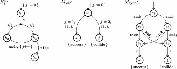
VMDP modelling hosts (\(H\)) that send on a shared medium (\(M\))
By abuse of language, we use the word “transition” when we actually mean “equivalence class of transitions under \(\equiv \)”.
Our implementation in modes therefore uses large default values for \(k_{\mathrm{max}}\) and \(l\) so the user usually need not worry about these parameters. If SMC aborts, the cause and its location is reported, including how it was detected, which may be that \(k_{\mathrm{max}}\) or \(l\) was exceeded.
For the CSMA/CD models, the state space sizes reported are for the digital clocks semantics of the PTA created by mcpta and thus not directly comparable to the state spaces modes works on.

References
Agresti, A., Coull, B.A.: Approximate is better than “exact” for interval estimation of binomial proportions. Am. Stat. 52(2), 119–126 (1998)
Andel, T.R., Yasinsac, A.: On the credibility of MANET simulations. IEEE Comput. 39(7), 48–54 (2006)
Baier, C., D’Argenio, P.R., Größer, M.: Partial order reduction for probabilistic branching time. Electron. Notes Theor. Comput. Sci. 153(2), 97–116 (2006)
Baier, C., Größer, M., Ciesinski, F.: Partial order reduction for probabilistic systems. In: QEST, pp. 230–239. IEEE Computer Society, New York (2004)
Baier, C., Katoen, J.-P.: Principles of Model Checking. MIT Press, Cambridge (2008)
Blom, S.: Partial \(\tau \)-confluence for efficient state space generation. Technical Report SEN-R0123, CWI (2001)
Blom, S., van de Pol, J.: State space reduction by proving confluence. In: Brinksma, E., Larsen, K.G. (eds.) CAV. Lecture Notes in Computer Science, vol. 2404, pp. 596–609. Springer, Berlin (2002)
Bogdoll, J., Fioriti, L.M.F., Hartmanns, A., Hermanns, H.: Partial order methods for statistical model checking and simulation. In: Bruni, R., Dingel, J. (eds.) FMOODS/FORTE. Lecture Notes in Computer Science, vol. 6722, pp. 59–74. Springer, Berlin (2011)
Bogdoll, J., Hartmanns, A., Hermanns, H.: Simulation and statistical model checking for modestly nondeterministic models. In: Schmitt, J.B. (ed.) MMB/DFT. Lecture Notes in Computer Science, vol. 7201, pp. 249–252. Springer, Berlin (2012)
Brázdil, T., Chatterjee, K., Chmelik, M., Forejt, V., Kretínský, J., Kwiatkowska, M.Z., Parker, D., Ujma, M.: Verification of Markov decision processes using learning algorithms. CoRR, abs/1402.2967 (2014)
Chaum, D.: The dining cryptographers problem: unconditional sender and recipient untraceability. J. Cryptol. 1(1), 65–75 (1988)
D’Argenio, P.R., Niebert, P.: Partial order reduction on concurrent probabilistic programs. In: QEST, pp. 240–249. IEEE Computer Society, New York (2004)
Evangelista, S., Pajault, C.: Solving the ignoring problem for partial order reduction. STTT 12(2), 155–170 (2010)
Forejt, V., Kwiatkowska, M.Z., Norman, G., Parker, D.: Automated verification techniques for probabilistic systems. In: Bernardo, M., Issarny, V. (eds.) SFM. Lecture Notes in Computer Science, vol. 6659, pp. 53–113. Springer, Berlin (2011)
Giro, S., D’Argenio, P.R., Fioriti, L.M.F.: Partial order reduction for probabilistic systems: a revision for distributed schedulers. In: Bravetti, M., Zavattaro, G. (eds.) CONCUR. Lecture Notes in Computer Science, vol. 5710, pp. 338–353. Springer, Berlin (2009)
Godefroid, P.: Partial-order methods for the verification of concurrent systems—an approach to the state-explosion problem. Lecture Notes in Computer Science, vol. 1032. Springer, Berlin (1996)
Groote, J.F., van de Pol, J.: State space reduction using partial tau-confluence. In: Nielsen, M., Rovan, B. (eds.) MFCS. Lecture Notes in Computer Science, vol. 1893, pp. 383–393. Springer, Berlin (2000)
Hansen, H., Kwiatkowska, M.Z., Qu, H.: Partial order reduction for model checking Markov decision processes under unconditional fairness. In: QEST, pp. 203–212. IEEE Computer Society, New York (2011)
Hansen, H., Timmer, M.: A comparison of confluence and ample sets in probabilistic and non-probabilistic branching time. Theor. Comput. Sci. 538C, 103–123 (2014)
Hartmanns, A., Hermanns, H.: A modest approach to checking probabilistic timed automata. In: QEST, pp. 187–196. IEEE Computer Society, New York (2009)
Hartmanns, A., Hermanns, H.: The modest toolset: an integrated environment for quantitative modelling and verification. In: Ábrahám, E., Havelund, K. (eds.) TACAS. Lecture Notes in Computer Science, vol. 8413, pp. 593–598. Springer, Berlin (2014)
Hartmanns, A., Timmer, M.: On-the-fly confluence detection for statistical model checking. In: Brat, G., Rungta, N., Venet, A. (eds.) NASA Formal Methods. Lecture Notes in Computer Science, vol. 7871, pp. 337–351. Springer, Berlin (2013)
Henriques, D., Martins, J., Zuliani, P., Platzer, A., Clarke, E.M.: Statistical model checking for Markov decision processes. In: QEST, pp. 84–93. IEEE Computer Society, New York (2012)
Hérault, T., Lassaigne, R., Magniette, F., Peyronnet, S.: Approximate probabilistic model checking. In: Steffen, B., Levi, G. (eds.) VMCAI. Lecture Notes in Computer Science, vol. 2937, pp. 73–84. Springer, Berlin (2004)
Hoeffding, W.: Probability inequalities for sums of bounded random variables. J. Am. Stat. Assoc. 58(301), 13–30 (1963)
Kwiatkowska, M.Z., Norman, G., Parker, D.: PRISM 4.0: Verification of probabilistic real-time systems. In: Gopalakrishnan, G., Qadeer, S. (eds.) CAV. LNCS, vol. 6806, pp. 585–591. Springer, Berlin (2011)
Lassaigne, R., Peyronnet, S.: Approximate planning and verification for large Markov decision processes. In: Ossowski, S., Lecca, P. (eds.) SAC, pp. 1314–1319. ACM, New York (2012)
Legay, A., Delahaye, B., Bensalem, S.: Statistical model checking: an overview. In: Barringer, H., Falcone, Y., Finkbeiner, B., Havelund, K., Lee, I., Pace, G.J., Rosu, G., Sokolsky, O., Tillmann, N. (eds.) RV. Lecture Notes in Computer Science, vol. 6418, pp. 122–135. Springer, Berlin (2010)
Legay, A., Sedwards, S.: Lightweight Monte Carlo algorithm for Markov decision processes. CoRR, abs/1310.3609 (2013)
Mateescu, R., Wijs, A.: Sequential and distributed on-the-fly computation of weak tau-confluence. Sci. Comput. Program. 77(10–11), 1075–1094 (2012)
Nimal, V.: Statistical approaches for probabilistic model checking. Master’s thesis, Oxford University (2010)
Pace, G.J., Lang, F., Mateescu, R.: Calculating-confluence compositionally. In: Hunt Jr., W.A., Somenzi, F. (eds.) CAV. Lecture Notes in Computer Science, vol. 2725, pp. 446–459. Springer, Berlin (2003)
Peled, D.: Combining partial order reductions with on-the-fly model-checking. In: Dill, D.L. (ed.) CAV. Lecture Notes in Computer Science, vol. 818, pp. 377–390. Springer, Berlin (1994)
Peled, D.: Combining partial order reductions with on-the-fly model-checking. Formal Methods Syst. Des. 8(1), 39–64 (1996)
Ross, S.M.: Simulation, 4th edn. Elsevier Academic Press, Amsterdam (2006)
Timmer, M.: Efficient Modelling, Generation and Analysis of Markov Automata. PhD thesis, University of Twente, The Netherlands (2013)
Timmer, M., Stoelinga, M., van de Pol, J.: Confluence reduction for probabilistic systems. In: Abdulla, P.A., Rustan, K., Leino, M. (eds.) TACAS. Lecture Notes in Computer Science, vol. 6605, pp. 311–325. Springer, Berlin (2011)
Timmer, M., van de Pol, J., Stoelinga, M.: Confluence reduction for Markov automata. In: Braberman, V.A., Fribourg, L. (eds.) FORMATS. Lecture Notes in Computer Science, vol. 8053, pp. 243–257. Springer, Berlin (2013)
Valmari, A.: A stubborn attack on state explosion. In: Clarke, E.M., Kurshan, R.P. (eds.) CAV. Lecture Notes in Computer Science, vol. 531, pp. 156–165. Springer, Berlin (1990)
Younes, H.L.S., Kwiatkowska, M.Z., Norman, G., Parker, D.: Numerical vs. statistical probabilistic model checking. STTT 8(3), 216–228 (2006)
Younes, H.L.S., Simmons, R.G.: Probabilistic verification of discrete event systems using acceptance sampling. In: Brinksma, E., Larsen, K.G. (eds.) CAV. Lecture Notes in Computer Science, vol. 2404, pp. 223–235. Springer, Berlin (2002)
Acknowledgments
This work was supported by the Transregional Collaborative Research Centre SFB/TR 14 AVACS, by the NWO-DFG bilateral project ROCKS, by the 7th EU Framework Programme under grant agreements 295261 (MEALS) and 318490 (SENSATION), by NWO under grant 612.063.817 (SYRUP), and by the CAS/SAFEA International Partnership Program for Creative Research Teams.
Author information
Authors and Affiliations
Corresponding author
Rights and permissions
About this article

Cite this article
Hartmanns, A., Timmer, M. Sound statistical model checking for MDP using partial order and confluence reduction. Int J Softw Tools Technol Transfer 17, 429–456 (2015). https://doi.org/10.1007/s10009-014-0349-7
Published:
Issue Date:
DOI: https://doi.org/10.1007/s10009-014-0349-7