Incomplete financial markets with real assets and wealth-dependent credit limits

Abstract

In this paper we analyze the effects of restricted participation in a two-period general equilibrium model with incomplete financial markets and two key elements: the competitive trading of real assets, i.e., assets having payouts in terms of vectors of commodities, and household-specific inequality constraints that restrict participation in the financial markets. Similar to certain arrangements in the market for bank loans, household borrowing is restricted by a household-specific wealth dependent upper bound on credit lines in all states of uncertainty in the second period. We first establish that, generically in the set of the economies, equilibria exist and are finite and regular. We then show that equilibria are generically suboptimal. Finally, we provide a robust example demonstrating that the equilibrium allocations can be Pareto improved through a tightening of the participation constraints. This suggests, contrary to what is often cited as economic wisdom in the popular press, that in a setting with frictions resulting in an inefficient allocation the regulation of markets may have a Pareto-improving effect on the economy.

1 Introduction

In this paper we analyze a two-period general equilibrium model with incomplete financial markets and two key elements: (1) the competitive trading of real assets, where real assets have payouts in terms of vectors of commodities, and (2) household-specific inequality constraints that restrict participation in the financial markets.

A formal introduction of time and uncertainty in a general equilibrium model dates back to Chapter 7 of “Theory of Value” by Debreu (1959). There, it is observed that enlarging the concept of commodity in order to include not only its physical and chemical characteristics, but also its location in space, time and state of the world, it is possible to show that existence and Pareto optimality of equilibria still hold true. In other words, those standard general equilibrium results can be obtained assuming the presence of markets in which all commodities, in the loose sense defined by Debreu, can be exchanged.

Arrow (1964)’s contribution is to observe that, while it is hard to believe that assumption is satisfied, it can probably be assumed that there exist sufficiently diversified and numerous available assets which are able to behave as well as those plethora of markets: indeed, equilibrium allocations in a market a la Debreu are the same as equilibria with commodity markets opening only inside each state of the world and enough available assets. On the other hand, it can also be claimed that in a quite uncertain world, available assets are not enough to insure against each possible future event: financial markets and, therefore, commodity a la Debreu markets, may be incomplete. That observation led to an important literature which focuses on the validity, in that more general and realistic environment, of the three main results in general equilibrium theory: existence, Pareto optimality and generic regularity of equilibria. While the first result is a sort of consistency check of the model and the second one is one of the main goal of economic analysis, the importance of the third, apparently only technical, result lies in the fact that it is the preliminary, indispensable tool for the analysis of existence of second best equilibria and of the chance of success of economic policies—see for example Chapter 15 in Villanacci et al. (2002). Indeed, the validity of the three above results was analyzed in the incomplete market framework with respect to some abstract types of assets, usually denoted in the literature as nominal, numeraire and real assets. Nominal assets promise to deliver units of account; real assets a bundle of goods; and numeraire assets just some amount of a given good, the so called numeraire good.

Each of the three main results of the general equilibrium model fails to hold true in one or more of the above defined types of incomplete market frameworks, as roughly summarized in the following table

(1)

where “Yes” means “it is always insured”, “Yes*” means “it is generically,¹ but not always insured” , and “No*” means “it is generically not insured”.²

Two important constructive criticisms to the model of incomplete markets, concerning the absence of restricted participation and of default possibilities, led to more general and realistic models [see for instance Seghir and Torres-Martinez (2011) and Geanakoplos and Zame (2014)].

“While there might be some disagreement over whether, in a modern developed economy, financial markets are actually incomplete, there can hardly be any disagreement over whether at least some economic agents are variously constrained in transacting on those financial markets” (Cass 1992). In other words, financial markets may be complete, but households surely face a personalized and restricted access to financial markets.

The literature on possibility of default removes the assumption that agents always honor their financial obligations. This literature has a basic link with the literature on restricted participation. It is indeed usually assumed that some commodity and/or financial collateral is required to partially counteract the damages of default. The corresponding conditions to be added to the standard model with incomplete markets make the model of default (and collateral) as a particular model of restricted participation with real assets. While existence and (lack of) Pareto optimality have been proved in such contexts, the existing literature has little to say about generic regularity in those models. The general goal of our paper is to study that problem.

Indeed, apart from the seminal paper by Radner (1972), “ universal” ³ existence proofs can be found in Geanakoplos and Zame (2014) in the case of collateral constraints, as well as in Seghir and Torres-Martinez (2011) and in Gori et al. (2013) in the case of financial constraints depending on some endogenous variables. The main limitation of those results is that the analytical methods used there seem unable to verify other equilibrium properties. By contrast, the technique we use to guarantee generic regularity also verifies the generic existence⁴ of an equilibrium, the generic (Pareto) suboptimality of the equilibrium allocations, and ensures that numerical methods [see Kubler (2007), for example] can be used to compute equilibria.

To the best of our knowledge, the only model of restricted participation with real assets in which generic regularity is proven is the one by Polemarchakis and Siconolfi (1997). Yet, in that paper, the restriction sets for the asset choices are difficult to interpret. Specifically, each household is exogenously associated with a linear subspace of the possible wealth transfers. Its restriction set is then described by the orthogonal projection of that subspace on the (price dependent) image of the return matrix. We are unable to provide an economic interpretation of that modeling choice and the authors themselves provide no explanation at all.

What we offer is an analysis of economically meaningful constraints on households’ participation in financial markets and a general approach to determine which constraints can be analyzed in a real asset setting.

The participation constraints described in our model, consistent with what occurs in the market for bank loans, impose an upper bound, called credit limit, on a household’s future debt in all states of uncertainty in the final period. A credit limit is the maximum amount that a household is allowed to borrow.⁵ It is an assessment of a prospective borrower to determine the likelihood that she will default on debts. For example, it is the most that a credit card company will allow a card holder to take out on a credit card in a given period of time. This limit is based on the household’s credit risk, which depends on a range of factors, such as her employment stability, level of income, level of debt, credit history. Households with a higher expected wealth will generally be loaned more money, that is, have a higher credit limit. In other words, there are two components to credit worthiness. One is a borrower’s current and projected ability to repay a loan or offer of credit. This can be determined by looking at things like income, other debts the borrower is carrying, expenses, and future employment opportunities. Another issue is the borrower’s inclination to repay debts, a surely more complicated matter. Some negative signals on that inclination are repeated delinquencies on other debts, sluggish repayment of loans, and other entries in a borrower’s credit history. One tool lenders can use to quickly assess credit worthiness is to consult a credit rating agency. These agencies monitor consumers and keep track of their financial activities to generate a credit score. Such rating is often used as a device to set credit limits. Credit limits provide some important advantages. For example, they serve to protect the borrower from borrowing too much money, and they also protect the lender from being over exposed to borrower’s getting too far into debt. Credit limits may however cause some disadvantages. For example, they may severely restrict the borrowing capacity of the borrower, reducing the value of items that they can purchase. As a result, credit limits can also reduce the potential income received by the lender because borrowers are limited in what they can borrow.

Our goal is to model the above economic observations in a general equilibrium model with two periods of time and absence of default. To formalize both components describing how credit limits are determined (credit risk and inclination to repay) we proceed as follows. The amount each household can borrow must be such that the household can repay what is due in all states in the final period. Additionally, each household is assumed not being able or willing to consume less than a given proportion of her wealth in each state in the second period. Those requirements lead to a household specific wealth-dependent credit limit, formalized in the borrowing constraint in (7).⁶

For our model, we show generic existence of equilibria and generic regularity, the latter being an indispensable tool to both describe equilibria and to prove several important normative properties of equilibria.

The first property we prove is that the equilibra are generically suboptimal. Additionally, we conjecture that a form of generic constrained suboptimality holds. We are verifying this conjecture in a companion paper, in which we restrict attention to the significant set of economies in which a sufficiently high number of participation constraints are binding. Generically in that set of economies, these equilibria are Pareto improvable through a local change of the participation constraints. The general strategy that is used in that framework is described in Carosi et al. (2009).

In the current paper, we describe a more direct approach to constrained suboptimality for a specific economy. Our contribution is in line with a general viewpoint dating back to what is usually mentioned as Lipsey–Lancaster theory of second best—see Lipsey and Lancaster (1956), according to which an increase in the level of a market imperfection may lead to a Pareto improvement. In the framework of incomplete markets, Hart (1975) showed that decreasing the number of available assets, and thus increasing the incompleteness of the markets, may increase efficiency. We rephrase and show the Lipsey-Lancaster claim in our model of restricted participation on financial markets. Indeed, we present a robust example in the economy space whose associated equilibria are such that using a more restrictive credit policy results in a Pareto improvement.

Without exaggerating the importance of a robust example, we do believe that the presented one supports two simple ideas. First of all, it shows the importance of general equilibrium analysis, i.e., the fact that price effects are able to more than welfare compensate a reduction of available choices. Moreover, it suggests, contrary to what is often cited as economic wisdom in the popular press, that in a setting with frictions resulting in an inefficient allocation, the regulation of markets may have a Pareto-improving effect on the economy.

We think our analysis contains both technically and economically significant features. We first discuss our technical contributions to the analysis of the problem of generic existence and generic regularity of equilibria.

The seminal contribution for generic existence in a model with real assets is the paper by Duffie and Shafer (1985). To prove generic existence, they first set the dimension of the return space equal to the number of available assets, define the resulting equilibrium a “pseudo equilibrium”, and show the existence of such an equilibrium. Finally, they prove that these pseudo equilibria are true equilibria for a generic subset of household endowments and asset payouts. With the inequality constraints that we use to model households’ restricted participation, the household demand functions are in general not $C^{1},$ and therefore the equilibrium manifold is not $C^{1}$ either. This fact prevents us from using the smooth analysis arguments in Duffie and Shafer (1985). Rather, we employ a fixed point argument based on the approach by Dierker (1974) for the Walrasian model and later generalized and formalized by Husseini et al. (1990) for the incomplete markets model with real assets. To the best of our knowledge, we provide the first application of the methodology in Husseini et al. (1990).

Duffie and Shafer (1985) use a “fixed dimension return space” approach⁷ with results in terms of the kernel of a well chosen linear function. In our model, characterizing equilibria using that approach would allow us to verify the existence of appropriately defined pseudo equilibria, but we are then unable to show that the pseudo equilibria are generically true equilibria.⁸ To circumvent this problem, we take a different approach by presenting a natural characterization of equilibria in terms of the image of an appropriately chosen linear function.

For those interested in the technical aspects of our proof,⁹ we preview the strategy used to obtain the generic existence result. As previously discussed, once the definition of equilibrium is introduced, we define a type of equilibrium in which we fix the dimension of the return space. Then, as done in the approach followed by Duffie and Shafer (1985), we use a Mr. 1 trick,¹⁰ i.e., we get rid of the explicit presence of the financial side of the economy using the introduction of a specific household, Mr. 1, who behaves as a Walrasian consumer. After showing that the latter two concepts are equivalent, we prove that they are a “true” equilibrium if a (standard) full rank condition of the return matrix holds true—see Proposition 9.

The technical reason to introduce two different types of auxiliary equilibria is described by the following logic. Using the approach by Dierker (1974) in the form of the theorem proved by Husseini et al. (1990), we are able to show the existence of a Mr. 1 equilibrium. Yet, as mentioned above, we are then unable to complete the next step as we are unable to verify that the projection function from the equilibrium set to the economy space is proper. This is a required step for the genericity argument. We can verify properness by using the equivalent concept of (normalized price) symmetric equilibrium in Definition 6.

We now discuss the economically significant features of both our model and our proof methodology. In terms of the type of participation constraints we employ, we believe they are realistic and economically meaningful. They are meant to represent the market for bank loans. Consider that legal requirements (or uncontractable social norms) are present that guarantee households a base level of consumption expenditure. Thus, for all states of uncertainty, a household is only able to repay previous debts if this leaves the household with at least this base level of consumption expenditure. Knowing this, the financial markets only permit borrowing up the point where the household is able to repay the loan and not be reduced to consumption expenditure below the base level.

To show the economic relevance of the constraints, we consider a simple example of our model. For the particular economy chosen, the equilibrium allocation can be Pareto improved by tightening the participation constraints in some states, without loosening the participation constraints in any other states, for all households. This result may seem counter-intuitive, but demonstrates the importance of general equilibrium price effects in financial markets. Thus, restricting credit access may in fact make all households better off.

More generally, the analysis presented in the paper provides what we believe are crucial conditions on the type of constraints for which generic regularity can be verified, at least following what currently seems to be the only successful approach: the fixed dimension return space approach. As will be discussed further in Sect. 2,¹¹ both the kernel approach [that is used in Duffie and Shafer (1985)] and the image approach (that we use here) require that the constraints on the financial side of the economy are rewritten in terms of constraints on the real side, specifically in terms of the values of the excess demands in each state. In the former approach, the financial side simply disappears from the household maximization problems. In the latter one, we must introduce fictitious asset demands and we recognize that constraints imposed on the fictitious asset demands may not be equivalent to constraints imposed on the true asset demands.

Future research is required to confirm this conjecture about the type of constraints that can be employed in models with real assets. Given this negative result, any attempts to obtain regularity for interesting models of collateral and default may be in vain. The reason is that any known approaches to modeling collateral and default involve restrictions that differ from the types of restrictions that we described above as being successful. Again, future research is required in this direction.

The rest of the paper is organized as follows. In Sect. 2, we present the set up of the model. In Sect. 3, we introduce some equivalent definitions of equilibria with fixed dimension of the return space. In Sect. 4, we state the results of existence of these equilibria, together with the generic existence, generic regularity and generic suboptimality of true equilibria. Section 5 contains the numerical example and the Appendix collects the proofs of Theorems 13 and 14.

2 Set up of the model

Our model builds on the standard two-period, general equilibrium model of pure exchange with uncertainty. In the commodity markets, $C\ge 2$ different physical commodities are traded, denoted by $c\in \fancyscript{C} =\{1,2,\dots ,C\}.$ In the final period, only one among $S\ge 1$ possible states of the world, denoted by $s\in \{1,2,\dots ,S\}$, will occur. The initial period is denoted $s=0$ and we define the set of all states $\fancyscript{S}=\{0,1,\dots ,S\}$ and the set of uncertain states $\fancyscript{S} ^{\prime }=\{1,\dots ,S\}.$ In the initial period, asset markets open and $A\ge 1$ assets are traded, denoted by $a\in \fancyscript{A}=\{1,2,\dots ,A\}.$

We assume $A\le S.$ Finally, there are $H\ge 2$ households, denoted by $h\in \fancyscript{H}=\{1,2,\dots ,H\}.$ The time structure of the model is as follows: in the initial period, households exchange commodities and assets, and consumption takes place. In the final period, uncertainty is resolved, households honor their financial obligations, exchange commodities, and then consume commodities.

We denote ${x}_{h}^{c}(s)\in \mathbb {R}_{++}$ and ${e}_{h}^{c}(s)\in \mathbb {R}_{++}$ as the consumption and the endowment of commodity $c$ in state $s$ by household $h,$ respectively.¹² We define $\mathbf {x}_{h}(s)=({x}_{h}^{c}(s))_{c\in \fancyscript{C}}\in \mathbb {R}_{++}^{C},\$ $\mathbf {x}_{h}=(\mathbf {x}_{h}(s))_{s\in \fancyscript{S}}\in \mathbb {R} _{++}^{G},\ \mathbf {x}=(\mathbf {x}_{h})_{h\in \fancyscript{H}}\in \mathbb {R}_{++}^{GH}$ and similarly $\mathbf {e}_{h}(s)\in \mathbb {R}_{++}^{C},\,\mathbf {e}_{h}\in \mathbb {R}_{++}^{G},\,\mathbf {e}\in \mathbb {R}_{++}^{GH},$ where $G=C(S+1).$

Household $h$’s preferences are represented by a utility function $u_{h}: \mathbb {R}_{++}^{G}\rightarrow \mathbb {R}$. As in most of the literature on smooth economies we assume that, for every $h\in \fancyscript{H}$,

$$\begin{aligned}&u_{h}\in C^{2}(\mathbb {R}_{++}^{G}); \end{aligned}$$

(2)

$$\begin{aligned}&\text{ for } \text{ every } \mathbf {x}_{h}\in \mathbb {R}_{++}^{G},\;\mathbf {Du}_{h}(\mathbf {x}_{h})\gg \mathbf {0}; \end{aligned}$$

(3)

$$\begin{aligned}&\text{ for } \text{ every } \mathbf {v}\in \mathbb {R}^{G}\setminus \{0\}\quad \text{ and } \quad \mathbf {x}_{h}\in \mathbb {R}_{++}^{G},\;\mathbf {v}\,\mathbf {D^{2}u}_{h}(\mathbf {x}_{h})\,\mathbf {v}<0\,; \end{aligned}$$

(4)

$$\begin{aligned}&\text{ for } \text{ every } \underline{\mathbf {x}}_{h}\in \mathbb {R}_{++}^{G},\;\left\{ \mathbf {x}_{h}\in \mathbb {R}_{++}^{G}:u_{h}(\mathbf {x}_{h})\ge u_{h}(\underline{\mathbf {x}}_{h})\right\} \text{ is } \text{ closed } \text{ in } \text{ the } \text{ Euclidean }\nonumber \\&\text{ topology } \text{ of } \mathbb {R}^{G}. \end{aligned}$$

(5)

Let us denote by $\fancyscript{U}$ the set of vectors $\mathbf {u}=(u_{h})_{h\in \fancyscript{H }}$ of utility functions satisfying assumptions (2), (3), (4), and (5). We denote by ${p}^{c}(s)\in \mathbb {R}_{++}$ the price of commodity $c$ in state $s$, by ${q}^{a}\in \mathbb {R}$ the price of asset $a$ and by ${b}_{h}^{a}\in \mathbb {R}$ the quantity of asset $a$ held by household $h$. Moreover we define $\mathbf {p}(s)=({p}^{c}(s))_{c\in \fancyscript{C}}\in \mathbb {R} _{++}^{C},\,\mathbf {p}=(\mathbf {p}(s))_{s\in \fancyscript{S}}\in \mathbb {R}_{++}^{G},\mathbf {q}=({q}^{a})_{a\in \fancyscript{A}}\in \mathbb {R}^{A},\,\mathbf {b}_{h}=({b}_{h}^{a})_{a\in \fancyscript{A}}\in \mathbb {R}^{A},\,\mathbf {b}=(\mathbf {b}_{h})_{h\in \fancyscript{H}}\in \mathbb {R}^{AH}.$

We denote by ${y}^{a,c}(s)\in \mathbb {R}$ the units of commodity $c$ delivered by one unit of asset $a$ in state $s$ and we define $\mathbf {y}^{a}(s)=({y}^{a,c}(s))_{c\in \fancyscript{C}}\in \mathbb {R}^{C},\,\mathbf {y}(s)=\left( \mathbf {y}^{a}(s)\right) _{a\in \fancyscript{A} }\in \mathbb {R}^{CA},\mathbf {y}=(\mathbf {y}(s))_{s\in \fancyscript{S}^{\prime }}\in \mathbb {R} ^{CAS}.$ ¹³ Note in particular that, in state $s$, asset $a$ promises to deliver a vector $\mathbf {y}^{a}(s)$ of commodities.

For any $m,n\in \mathbb {N}\setminus \{0\}$, let $\mathbb {M}\left( m,n\right)$ be the set of real $m\times n$ matrices and $\mathbb {M}^{f}\left( m,n\right)$ be the set of real $m\times n$ matrices with full rank. Define the return matrix function as follows

$$\begin{aligned} \fancyscript{R}:\mathbb {R}_{++}^{G}\times \mathbb {R}^{CAS}\rightarrow \mathbb {M} (S,A), \end{aligned}$$

$$\begin{aligned} \begin{array}{l} (\mathbf {p},\mathbf {y})\mapsto \left[ \begin{array}{lllll} \mathbf {p}(1)\mathbf {y}^{1}(1) &{} \ldots &{} \mathbf {p}(1)\mathbf {y}^{a}(1) &{} \ldots &{} \mathbf {p}(1)\mathbf {y}^{A}(1) \\ \vdots &{} \ddots &{} \vdots &{} \ddots &{} \vdots \\ \mathbf {p}(s)\mathbf {y}^{1}(s) &{} \ldots &{} \mathbf {p}(s)\mathbf {y}^{a}(s) &{} \ldots &{} \mathbf {p}(s)\mathbf {y}^{A}(s) \\ \vdots &{} \ddots &{} \vdots &{} \ddots &{} \vdots \\ \mathbf {p}(S)\mathbf {y}^{1}(S) &{} \ldots &{} \mathbf {p}(S)\mathbf {y}^{a}(S) &{} \ldots &{} \mathbf {p}(S)\mathbf {y}^{A}(S) \end{array} \right] = \left[ \begin{array}{l} \mathbf {r}^{1}(\mathbf {p},\mathbf {y}) \\ \vdots \\ \mathbf {r}^{s}(\mathbf {p},\mathbf {y}) \\ \vdots \\ \mathbf {r}^{S}(\mathbf {p},\mathbf {y}) \end{array} \right] . \end{array} \end{aligned}$$

For future use we also define, for every $\mathbf {p}\in \mathbb {R}^G_{++},$

$$\begin{aligned} {\varPhi } \left( \mathbf {p}\right) =\left[ \begin{array}{llll} \mathbf {p}\left( 0\right) &{} &{} &{} \\ &{} \mathbf {p}\left( 1\right) &{} &{} \\ &{} &{} \ddots &{} \\ &{} &{} &{} \mathbf {p}\left( S\right) \end{array} \right] \in \mathbb {M}(S+1,G). \end{aligned}$$

Mimicking what happens in the market for bank loans, the constraints that we impose are credit limits which bound the amount of future debt of the borrower, proportionally to his/her credit worthiness. In fact, we say that the amount household $h$ can borrow, i.e., $\mathbf {q}\ \left( -\mathbf {b}_{h}\right)$, must be such that the household can repay what is due in all states in the final period. That amount due is

$$\begin{aligned} \mathbf {r}^{s}\left( \mathbf {p},\mathbf {y}\right) \left( -\mathbf {b}_{h}\right) ,\quad \forall s\in \fancyscript{S} ^{\prime }. \end{aligned}$$

(6)

Additionally, we assume that each household will not be able (due to legal restrictions) or will not be willing to consume less than a given proportion $\gamma _{h}\left( s\right)$ of its wealth in state $s\in \fancyscript{S} ^{\prime }.$ In other words, there is a base level of consumption expenditure required for all households:

$$\begin{aligned} \gamma _{h}\left( s\right) \mathbf {p}\left( s\right) \mathbf {e}_{h}\left( s\right) . \end{aligned}$$

Then we require that the amount due in (6) has to be smaller than the difference between a household’s endowment level and the base level of consumption expenditure:

$$\begin{aligned} \left( 1-\gamma _{h}\left( s\right) \right) \mathbf {p}\left( s\right) \mathbf {e}_{h}\left( s\right) . \end{aligned}$$

Therefore, defining $\alpha _{h}\left( s\right) =1-\gamma _{h}\left( s\right)$, the borrowing constraints we impose are¹⁴:

$$\begin{aligned} \forall h\in \fancyscript{H}, \quad \forall s\in \fancyscript{S}^{\prime },\quad -\mathbf {r}^{s}\left( \mathbf {p},\mathbf {y}\right) \mathbf {b}_{h}\le \alpha _{h}\left( s\right) \mathbf {p}\left( s\right) \mathbf {e}_{h}\left( s\right) , \end{aligned}$$

(7)

where $\alpha _{h}\left( s\right) \in \left( 0,1\right) , \forall h\in \fancyscript{H}$ and $\forall s\in \fancyscript{S}^{\prime }.$

Including the participation constraint parameters along with the parameters governing the asset structure and the household endowments and preferences, we define the set of economies as

$$\begin{aligned} \fancyscript{E}=\mathbb {R}_{++}^{GH}\times \fancyscript{U}\times \mathbb {R}^{CAS}\times \left( 0,1\right) ^{SH}, \end{aligned}$$

with generic element $\left( \mathbf {e},\mathbf {u},\mathbf {y},\mathbf {\alpha } \right) ,$ where $\mathbf {\alpha } =(\mathbf {\alpha } _{h})_{h\in \fancyscript{H}}=(\alpha _{h}(s))_{h\in \fancyscript{H},s\in \fancyscript{S} ^{\prime }}.$

Definition 1

A vector $\left( \mathbf {x}^{*},\mathbf {p}^{*},\mathbf {b}^{*},\mathbf {q}^{*}\right)$ $\in \mathbb {R}_{++}^{GH}\times \mathbb {R}_{++}^{G}\times \mathbb {R}^{AH}$ $\times \mathbb {R}^{A}$ is an equilibrium for the economy $\left( \mathbf {e},\mathbf {u},\mathbf {y},\mathbf {\alpha } \right) \in \fancyscript{E}$ if

• 1. $\forall h\in \fancyscript{H},\;\left( \mathbf {x}_{h}^{*},\mathbf {b}_{h}^{*}\right)$ solves the following problem: given $\left( \mathbf {p}^{*},\mathbf {q}^{*},\mathbf {e},\mathbf {u},\mathbf {y},\mathbf {\alpha } \right)$

  $$\begin{aligned}&\underset{\left( \mathbf {x}_{h},\mathbf {b}_{h}\right) \in \mathbb {R}_{++}^{G}\times \mathbb {R}^{A}}{\max }u_{h}\left( \mathbf {x}_{h}\right) \nonumber \\&s.t. \mathbf {p}^{*}\left( 0\right) \left( \mathbf {x}_{h}\left( 0\right) -\mathbf {e}_{h}\left( 0\right) \right) +\mathbf {q}^{*}\mathbf {b}_{h}\le 0 \end{aligned}$$

  (8a)
  $$\begin{aligned}&\mathbf {p}^{*}\left( s\right) \left( \mathbf {x}_{h}\left( s\right) -\mathbf {e}_{h}\left( s\right) \right) -\left( \mathbf {p}^{*}\left( s\right) \mathbf {y}^{a}\left( s\right) \right) _{a=1}^{A}\mathbf {b}_{h}\le 0,\quad \forall s\in \fancyscript{S}^{\prime } \end{aligned}$$

  (8b)
  $$\begin{aligned}&-\left( \mathbf {p}^{*}\left( s\right) \mathbf {y}^{a}\left( s\right) \right) _{a=1}^{A}\mathbf {b}_{h}\le \alpha _{h}\left( s\right) \mathbf {p}^{*}\left( s\right) \mathbf {e}_{h}\left( s\right) ,\quad \forall s\in \fancyscript{S}^{\prime } \end{aligned}$$

  (8c)

• 2. $\left( \mathbf {x}^{*},\mathbf {b}^{*}\right)$ satisfies the market clearing conditions

  $$\begin{aligned} \sum _{h=1}^{H}\left( \mathbf {x}_{h}^{*}-\mathbf {e}_{h}\right) =\mathbf {0} \end{aligned}$$

  (9)

  and

  $$\begin{aligned} \sum _{h=1}^{H}\mathbf {b}_{h}^{*}=\mathbf {0}. \end{aligned}$$

  (10)

Define

$$\begin{aligned} \mathbf {p}^{\backslash }\left( s\right) =\left( p^{c}\left( s\right) \right) _{c\ne 1}\in \mathbb {R}_{++}^{C-1},\text { for any }s\in \fancyscript{S},\,\text { and } \,\mathbf {p}^{\backslash }=\left( \mathbf {p}^{\backslash }\left( s\right) \right) _{s\in \fancyscript{S}}\in \mathbb {R}_{++}^{G-\left( S+1\right) }, \end{aligned}$$

and similarly, for any $h\in \fancyscript{H}$, $\mathbf {x}_{h}^{\backslash }(s),\, \mathbf {x}_{h}^{\backslash },\, \mathbf {e}_{h}^{\backslash }(s)$ and $\mathbf {e}_{h}^{\backslash }.$

Remark 2

Observe that the number of admissible price normalizations for the equilibrium concept presented above is $S+1$ (one for each spot) and there are $S+1$ Walras’ laws. Therefore, the number of significant equations [i.e., conditions (9) and (10) “without $S+1$ Walras’ laws”] is equal to the number of significant variables (i.e., spot by spot normalized good prices $\mathbf {p}^{\backslash }$ and asset prices $\mathbf {q}$).

The above observations are formalized in the following definition.

Definition 3

A vector $\left( \mathbf {x}^{*},\mathbf {p}^{\backslash *},\mathbf {b}^{*},\mathbf {q}^{*}\right)$ $\in \mathbb {R}_{++}^{GH}\times \mathbb {R} _{++}^{G-\left( S+1\right) }\times \mathbb {R}^{AH}\times \mathbb {R}^{A}$ is a normalized equilibrium for the economy $\left( \mathbf {e},\mathbf {u},\mathbf {y},\mathbf {\alpha } \right) \in \fancyscript{E}$ if

• 1. $\forall h\in \fancyscript{H}\ ,\;\left( \mathbf {x}_{h}^{*},\mathbf {b}_{h}^{*}\right)$ solves Problem (8) given $\left( \mathbf {p}^{*},\mathbf {q}^{*},\left( \mathbf {e},\mathbf {u},\mathbf {y},\mathbf {\alpha } \right) \right) ,$ where $\mathbf {p}^{*}=\left( 1,\mathbf {p}^{\backslash *}\left( s\right) \right) _{s=0}^{S};$

• 2. $\mathbf {b}^{*}$ satisfies market clearing conditions (10) and

  $$\begin{aligned} \sum _{h=1}^{H}\left( \mathbf {x}_{h}^{*\backslash }-\mathbf {e}_{h}^{\backslash }\right) =\mathbf {0}. \end{aligned}$$

Remark 4

We do distinguish between different normalizations because showing our results requires to carefully keep track of different normalizations for some of the introduced definitions of equilibria. Observe however that, similarly to what done below in the case of equilibria with fixed dimension of the return space in Proposition 8, it is easy to prove that an equilibrium according to Definition 1 and its normalized version in Definition 3 are allocation equivalent.

Let’s further consider the restrictions we chose to analyze and the technical reasons why these constraints can be analyzed using our proof methodology. From Duffie and Shafer (1985), the standard way to tackle the problem of generic existence of equilibria in the real asset model is to fix the dimension of the return space so that the return matrix does not suffer a drop in rank. We briefly describe this process. Define

$$\begin{aligned} \varPhi ^{\mathbf {1}}\left( \mathbf {p}\right) =\left[ \begin{array}{lll} \mathbf {p}\left( 1\right) &{} &{} \\ &{} \ddots &{} \\ &{} &{} \mathbf {p}\left( S\right) \end{array} \right] \quad \text{ and } \quad \mathbf {z}_{h}^{\mathbf {1}}=\mathbf {x}_{h}^{\mathbf {1} }-\mathbf {e}_{h}^{\mathbf {1}}, \end{aligned}$$

with $\mathbf {x}_{h}^{\mathbf {1}}=(\mathbf {x}_{h}(s))_{s\in \fancyscript{S}^{\prime }}\in \mathbb {R} _{++}^{{CS}}$ and $\mathbf {e}_{h}^{\mathbf {1}}=(\mathbf {e}_{h}(s))_{s\in \fancyscript{S}^{\prime }}\in \mathbb {R}_{++}^{{CS}}\,.$

In this fixed dimension return space approach, the budget constraints in the final period (8b) can be equivalently expressed as:

$$\begin{aligned} \varPhi ^{\mathbf {1}}\left( \mathbf {p}\right) \mathbf {z}_{h}^{\mathbf {1}}\in L, \end{aligned}$$

(11)

where $L\$is an $A$ dimensional subspace of $\mathbb {R}^{S}$. Condition (11) is equivalent to any of the following conditions:

• 1.
  $$\begin{aligned} \exists \mathbf {M}\left( L\right) \in \mathbb {M}^{f}\left( S-A,S\right) \hbox {such that } \mathbf {M}\left( L\right) \cdot \varPhi ^{\mathbf {1}}\left( \mathbf {p}\right) \mathbf {z}_{h}^{\mathbf {1} }=\mathbf {0}, \end{aligned}$$

  (12)

  where $\mathbf {M}(L)$ is such that $\ker \mathbf {M}\left( L\right) =L$;

• 2.
  $$\begin{aligned} \exists \mathbf {N}\left( L\right) \in \mathbb {M}^{f}\left( S,A\right) \, \mathrm{and}\, \exists \mathbf {b}_{h}\in \mathbb {R}^{A} \hbox {such that } \varPhi ^{\mathbf {1}}\left( \mathbf {p}\right) \mathbf {z}_{h}^{\mathbf {1}}=\mathbf {N}\left( L\right) \cdot \mathbf {b}_{h}, \end{aligned}$$

  (13)

  where $\mathbf {N}(L)$ is such that $\mathrm {Im}\,\mathbf {N}\left( L\right) =L$.

Duffie and Shafer (1985) use condition (12). Here, we use condition (13) as well. With either condition, it is not clear how to impose constraints directly on $\mathbf {b}_{h}$. In the first condition, $\mathbf {b}_{h}$ does not appear. In regard to the second condition, we show that for a “fictitious” (regular) equilibrium, up to permutations of states, there exists $\mathbf {E}\in \mathbb {M}\left( S-A,A\right)$ such that

$$\begin{aligned} \left[ \begin{array}{l} \mathbf {I} \\ \mathbf {E} \end{array} \right] \mathbf {b}_{h}=\fancyscript{R}(\mathbf {p},\mathbf {y})\mathbf {b}_{h}^{\prime }=\left[ \begin{array}{l} \mathbf {R}^{*}\left( \mathbf {p},\mathbf {y}\right) \\ \widehat{\mathbf {R}}\left( \mathbf {p},\mathbf {y}\right) \end{array} \right] \mathbf {b}_{h}^{\prime }, \end{aligned}$$

where $\mathbf {R}^{*}\left( \mathbf {p},\mathbf {y}\right)$ has full rank, $\mathbf {b}_{h}$ is the asset demand in a fictitious equilibrium, and $\mathbf {b}_{h}^{\prime }$ is the asset demand in the true equilibrium. Therefore, again up to permutations, we get that¹⁵

$$\begin{aligned} \mathbf {b}_{h}^{\prime }=\left[ \mathbf {R}^{*}\left( \mathbf {p},\mathbf {y}\right) \right] ^{-1}\mathbf {b}_{h}. \end{aligned}$$

The above condition indicates that imposing restrictions on the fictitious equilibrium asset demand $\mathbf {b}_{h}$ does not imply that the same restrictions will hold for the true asset demand $\mathbf {b}_{h}^{\prime }.$ For example, the restriction $\mathbf {b}_{h}\ge \mathbf {0}$ does not imply that $\mathbf {b}_{h}^{\prime }=\left[ \mathbf {R}^{*}\left( \mathbf {p},\mathbf {y}\right) \right] ^{-1}\mathbf {b}_{h}\ge \mathbf {0}$. That explains why the fixed dimension return space approach is likely not applicable for restrictions written directly in terms of $\mathbf {b}_{h}$.

On the other hand, constraints on the physical quantity $b_{h}^{a}$ have little meaning as the future yields depend upon future commodity prices. So constraints could be written for each asset on the value $q^{a}b_{h}^{a},$ but this presupposes that either lenders are not able to gain information about the other assets in a household’s portfolio or do not care about this information.

The latter assumption is absurd as future repayment likelihoods depend upon all asset positions of a household, while the former assumption imposes an unrealistic information gap in this market for bank loans. Thus, it appears more economically meaningful to consider constraints imposed upon the payouts of all assets of a household in the final period.¹⁶

Finally, our methods allow us to conjecture that [similarly to Polemarchakis and Siconolfi (1997)] restricting excess demand in all states to a linear subspace of the column span of the returns matrix also suffices to guarantee generic existence and regularity. The restriction that we have in mind is:

$$\begin{aligned} \varPhi ^{\mathbf {1}}\left( \mathbf {p}\right) \mathbf {z}_{h}^{\mathbf {1}}\in L_{h}\left( \mathbf {p}\right) , \end{aligned}$$

(14)

where $L_{h}\left( \mathbf {p}\right)$ is a household-specific price-dependent return space, which is a linear subspace of $L.$ The constraints of this form (14) fit with the fixed dimension return space approach, as we can simply replace $L$ in the previous analysis with $L_{h}\left( \mathbf {p}\right) .$ In fact, similar restrictions have been considered by Balasko et al. (1990), in the case of nominal assets. We do not consider constraints (14) any further in the present paper, but we are working with them in a companion paper.

3 Equilibria with fixed dimension of the return space

As explained in the previous sections, we present some definitions of equilibria in which the dimension of the feasible wealth transfer space $L$ is fixed and equal to the number of available assets, $A.$

The main difference between the concept of pseudo equilibrium in Duffie and Shafer (1985) and the one proposed below in Definitions 5 and 6 is that in the former the space $L$ appearing in the household maximization problem is written as the kernel of a linear function, while in our household maximization problem [see (16)] the space $L$ is the image of a linear function.

Below, after introducing some preliminary definitions and facts, we present three equivalent definitions of equilibria that are useful for our analysis. Indeed, as explained in Sect. 1, the different steps in the proofs of Theorems 13 and 14 require a different definition of equilibrium.

We denote by $\fancyscript{G}_{A,S}$ the set of $A$ dimensional vector subspaces of $\mathbb {R}^{S}$. It can be shown that $\fancyscript{G}_{A,S}$ is a Hausdorff, compact, and second countable (and therefore sequentially compact) metric space and also a $C^{\infty }$ abstract manifold of dimension $A\left( S-A\right)$.¹⁷

Denoting by $\Sigma$ the set of permutations of $\left\{ 1,\dots ,S\right\} ,$ with generic element $\sigma \in \Sigma ,$ by $\mathbf {P_{\sigma }}$ the corresponding permutation matrix and by $\mathbf {I}_{M}$ the $M$-dimensional identity matrix, then for every $L\in \fancyscript{G}_{A,S},$ there exists $\sigma ^{-1} \in \Sigma ,$ a neighborhood $V_{\sigma ^{-1}}$ of $L,$ and a diffeomorphism¹⁸

$$\begin{aligned} \psi _{{\sigma }^{-1}}:V_{{\sigma }^{-1}}\rightarrow \mathbb {M}\left( S-A,A\right) \end{aligned}$$

(15)

such that $L=\mathrm {Im}\,\mathbf {P_{\sigma }}\left[ \begin{array}{l} -\psi _{{\sigma }^{-1}}\left( L\right) \\ \mathbf {I}_{A} \end{array} \right] =\ker \left[ \mathbf {I}_{S-A}\ |\ \psi _{{\sigma }^{-1}}\left( L\right) \right] \cdot \mathbf {P_{\sigma ^{-1}}}.$

Define

$$\begin{aligned} \mathbf {A}_{h}=\left[ \begin{array}{lll} \alpha _{h}\left( 1\right) &{} &{} \\ &{} \ddots &{} \\ &{} &{} \alpha _{h}\left( S\right) \end{array} \right] . \end{aligned}$$

Definition 5

A vector $\left( \mathbf {x}^{*},\mathbf {p}^{*},\mathbf {b}^{*},\mathbf {q}^{*},L^{*}\right)$ $\in \mathbb {R}_{++}^{GH}\times \mathbb {R} _{++}^{G}\times \mathbb {R}^{AH}\times \mathbb {R}^{A}\times \fancyscript{G}_{A,S}$ is a symmetric equilibrium for the economy $\left( \mathbf {e},\mathbf {u},\mathbf {y},\mathbf {\alpha } \right) \in \fancyscript{E}$ if

• 1. $\forall h\in \fancyscript{H}\ ,\;\left( \mathbf {x}_{h}^{*},\mathbf {b}_{h}^{*}\right)$ solves the following problem:

  given $\left( \mathbf {p}^{*},\mathbf {q}^{*},L^{*},\mathbf {e},\mathbf {u},\mathbf {y},\mathbf {\alpha } \right)$

  $$\begin{aligned}& \underset{\left( \mathbf {x}_{h},\mathbf {b}_{h}\right) \in \mathbb {R}_{++}^{G}\times \mathbb {R} ^{A}}{\max }u_{h}\left( \mathbf {x}_{h}\right) \nonumber \\&s.t. -\mathbf {p}^{*}\left( 0\right) \left( \mathbf {x}_{h}\left( 0\right) -\mathbf {e}_{h}\left( 0\right) \right) -\mathbf {q}^{*}\mathbf {b}_{h}=0 \end{aligned}$$

  (16a)
  $$\begin{aligned}&-\varPhi ^{\mathbf {1}}\left( \mathbf {p}^{*}\right) \left( \mathbf {x}_{h}^{\mathbf {1} }-\mathbf {e}_{h}^{\mathbf {1}}\right) +\mathbf {P_{\sigma }}\left[ \begin{array}{l} -\psi \left( L^{*}\right) \\ \mathbf {I}_{A} \end{array} \right] \mathbf {b}_{h}=\mathbf {0} \end{aligned}$$

  (16b)
  $$\begin{aligned}&\mathbf {P_{\sigma }}\left[ \begin{array}{l} -\psi \left( L^{*}\right) \\ \mathbf {I}_{A} \end{array} \right] \mathbf {b}_{h}+\mathbf {A}_{h}\cdot \varPhi ^{\mathbf {1}}\left( \mathbf {p}^{*}\right) \mathbf {e}_{h}^{ \mathbf {1}}\ge \mathbf {0} \end{aligned}$$

  (16c)

• 2. $\left( \mathbf {x}^{*},\mathbf {b}^{*}\right)$ satisfies market clearing conditions (9) and (10);

• 3. $\mathrm {Im}\fancyscript{R}\left( \mathbf {p}^{*},\mathbf {y}\right) \subseteq L^{*},$ i.e.,

  $$\begin{aligned} \mathrm {vec}\left[ \mathbf {I}_{S-A}\ |\ \psi \left( L^{*}\right) \right] \cdot \mathbf {P_{\sigma ^{-1}}}\cdot \fancyscript{R}\left( \mathbf {p}^{*},\mathbf {y}\right) =\mathbf {0}. \end{aligned}$$

  (17)

Define $\varDelta _{++}^{G-1}=\big \{\mathbf {p}\in \mathbb {R}_{++}^{G}:\sum _{s=0}^{S}\sum _{c=1}^{C}p^{c}\left( s\right) =1\big \}$ and, for any $h\in \fancyscript{H}$, $\mathbf {e}_{h}^{\diamond }=\left( e_{h}^{1}\left( s\right) \right) _{s\in \fancyscript{S} }\in \mathbb {R}_{++}^{S+1},$ $\mathbf {e}_{h}^{\backslash \left( 01\right) }=\left( e_{h}^{c}\left( s\right) \right) _{(s,c)\ne (0,1)}\in \mathbb {R}_{++}^{G-1}, \, \mathbf {x}_{h}^{\backslash \left( 01\right) }=\left( x_{h}^{c}\left( s\right) \right) _{(s,c)\ne (0,1)}\in \mathbb {R}_{++}^{G-1}.$ Moreover, $\mathbf {1}_{N}$ denotes an $N$ dimensional vector whose components are all equal to $1$; if no confusion arises, we will write $\mathbf {1}$ in the place of $\mathbf {1}_{N}$.

As in the case of equilibria presented in Definition 1, we formalize the possibility of normalizing prices and the validity of Walras’ laws in Definition 6 below.

Definition 6

A vector $\left( \mathbf {x}^{*}, \mathbf {p}^{\backslash *},\mathbf {b}^{*},\mathbf {q}^{*},L^{*}\right)$ $\in \mathbb {R} _{++}^{GH}\times \mathbb {R}_{++}^{G-\left( S+1\right) }\times \mathbb {R} ^{AH}\times \mathbb {R}^{A}\times \fancyscript{G}_{A,S}$ is a normalized symmetric equilibrium for the economy $\left( \mathbf {e},\mathbf {u},\mathbf {y},\mathbf {\alpha } \right) \in \fancyscript{E}$ if

• 1. $\forall h\in \fancyscript{H}\ ,\;\left( \mathbf {x}_{h}^{*},\mathbf {b}_{h}^{*}\right)$ solves Problem (16) given $\left( \mathbf {p}^{*},\mathbf {q}^{*},L^{*},\left( \mathbf {e},\mathbf {u},\mathbf {y},\mathbf {\alpha } \right) \right) ,$ where $\mathbf {p}^{*}=\left( 1,\mathbf {p}^{\backslash *}\left( s\right) \right) _{s=0}^{S} ;$

• 2. $\mathbf {b}^{*}$ satisfies market clearing conditions (10) and

  $$\begin{aligned} \sum _{h=1}^{H}\left( \mathbf {x}_{h}^{*\backslash }-\mathbf {e}_{h}^{\backslash }\right) =\mathbf {0}; \end{aligned}$$

• 3. Condition (17) holds true.

We now introduce the needed definition of Mr. 1 equilibrium.

Definition 7

A vector $\left( \mathbf {x}^{*},\mathbf {p}^{*},L^{*}\right) \in \mathbb {R}_{++}^{GH}\times \varDelta _{++}^{G-1}\times \fancyscript{G}_{A,S}$ is a Mr. 1 equilibrium ¹⁹ for the economy $\left( \mathbf {e},\mathbf {u},\mathbf {y},\mathbf {\alpha } \right) \in \fancyscript{E}$ if

• 1a. $\forall h\in \fancyscript{H}\backslash \left\{ 1\right\} ,\;\mathbf {x}_{h}^{*}$ solves the following problem: given $\left( \mathbf {p}^{*},L^{*},\mathbf {e},\mathbf {u},\mathbf {y},\mathbf {\alpha } \right) ,$

  $$\begin{aligned} \underset{\mathbf {x}_{h}\in B_{h}^{\backslash \mathbf {b}}\left( \mathbf {p}^{*},L^{*}\right) }{ \max }u_{h}\left( \mathbf {x}_{h}\right) \end{aligned}$$

  (18)

  where $B_{h}^{\backslash \mathbf {b}}\left( \mathbf {p}^{*},L^{*}\right) =$

  $$\begin{aligned}&\bigg \{\mathbf {x}_{h}\in \mathbb {R}_{++}^{G}: \exists \mathbf {b}_{h}\in \mathbb {R}^{A}\text { such that} \nonumber \\&-\mathbf {p}^{*}\left( 0\right) \left( \mathbf {x}_{h}\left( 0\right) -\mathbf {e}_{h}\left( 0\right) \right) -\mathbf {1}\cdot \mathbf {P}_{\sigma }\left[ \begin{array}{l} -\psi \left( L^{*}\right) \\ \mathbf {I}_{A} \end{array} \right] \mathbf {b}_{h}=0 \end{aligned}$$

  (19a)
  $$\begin{aligned}&-\varPhi ^{\mathbf {1}}\left( \mathbf {p}^{*}\right) \left( \mathbf {x}_{h}^{\mathbf {1}}-\mathbf {e}_{h}^{\mathbf {1}}\right) +\mathbf {P}_{\sigma }\left[ \begin{array}{l} -\psi \left( L^{*}\right) \\ \mathbf {I}_{A} \end{array} \right] \mathbf {b}_{h}=\mathbf {0} \end{aligned}$$

  (19b)
  $$\begin{aligned}&\mathbf {P}_{\sigma }\left[ \begin{array}{l} -\psi \left( L^{*}\right) \\ \mathbf {I}_{A} \end{array} \right] \mathbf {b}_{h}+\mathbf {A}_{h}\varPhi ^{\mathbf {1}}\left( \mathbf {p}^{*}\right) \mathbf {e}_{h}^{\mathbf {1}}\ge \mathbf {0} \bigg \} \end{aligned}$$

  (19c)

• 1b. $\mathbf {x}_{1}^{*}$ solves the following problem: given $\left( \mathbf {p}^{*},L^{*},\mathbf {e},\mathbf {u},\mathbf {y},\mathbf {\alpha } \right) ,$

  $$\begin{aligned}&\underset{\mathbf {x}_{1}\in \mathbb {R}_{++}^{G}}{\max }u_{1}\left( \mathbf {x}_{1}\right) \nonumber \\&s.t. -\mathbf {p}^{*}\left( 0\right) \left( \mathbf {x}_{1}\left( 0\right) -\mathbf {e}_{1}\left( 0\right) \right) -\mathbf {1}\cdot \varPhi ^{\mathbf {1}}\left( \mathbf {p}^{*}\right) \left( \mathbf {x}_{1}^{\mathbf {1}}-\mathbf {e}_{1}^{\mathbf {1}}\right) =0 \end{aligned}$$

  (20a)
  $$\begin{aligned}&\varPhi ^{\mathbf {1}}\left( \mathbf {p}^{*}\right) \left( \mathbf {x}_{1}^{\mathbf {1}}-\mathbf {e}_{1}^{\mathbf {1}}\right) +\mathbf {A}_{1}\varPhi ^{\mathbf {1}}\left( \mathbf {p}^{*}\right) \mathbf {e}_{1}^{\mathbf {1}}\ge \mathbf {0} \end{aligned}$$

  (20b)

• 2. $\mathbf {x}^{*}$ satisfies market clearing conditions

  $$\begin{aligned} \sum _{h=1}^{H}\left( \mathbf {x}_{h}^{*\backslash \left( 01\right) }-\mathbf {e}_{h}^{\backslash \left( 01\right) }\right) =\mathbf {0}; \end{aligned}$$

  (21)

• 3. Condition (17) holds true.

Definitions 5, 6, and 7 are in fact “allocation equivalent”, as stated below.²⁰

Proposition 8

For a given economy $\left( \mathbf {e},\mathbf {u},\mathbf {y},\mathbf {\alpha } \right) \in \fancyscript{E},$ the following statements are equivalent:

• 1. $\mathbf {x}$ is a symmetric equilibrium allocation;

• 2. $\mathbf {x}$ is a normalized symmetric equilibrium allocation;

• 3. $\mathbf {x}$ is a Mr. 1 equilibrium allocation.

Proposition 9 describes the relationship between equilibria with fixed dimension of the return space and “true” equilibria.

Proposition 9

If $\left( \mathbf {x}^{*},\mathbf {p}^{\backslash *},\mathbf {b}^{*},\mathbf {q}^{*},L^{*}\right)$ $\in \mathbb {R}_{++}^{GH}\times \mathbb {R} _{++}^{G-\left( S+1\right) }\times \mathbb {R}^{AH}\times \mathbb {R} ^{A}\times \fancyscript{G}_{A,S}$ is a normalized symmetric equilibrium for the economy $\left( \mathbf {e},\mathbf {u},\mathbf {y},\mathbf {\alpha } \right) \in \fancyscript{E}$ and

$$\begin{aligned} \mathrm{rank} \fancyscript{R}\left( \mathbf {p}^{*},\mathbf {y}\right) =A, \end{aligned}$$

(22)

where $\mathbf {p}^{*}=\left( 1,\mathbf {p}^{\backslash *}\left( s\right) \right) _{s=0}^{S},$ then there exist $\mathbf {b}^{**}$ and $\mathbf {q}^{**}$ such that $\left( \mathbf {x}^{*},\mathbf {p}^{\backslash *},\mathbf {b}^{**},\mathbf {q}^{**}\right)$ is a normalized equilibrium for $\fancyscript{E}.$

Proof

See Hoelle et al. (2012).

4 Generic existence, regularity, and suboptimality

In this section, we first show existence of an Mr. 1 equilibrium—see Theorem 13. Then, we can obtain the generic existence of a true equilibrium, after showing the generic regularity and generic full rank condition of the return matrix for normalized symmetric equilibria—see Theorem 14.

As a preliminary step towards the application of a Brouwer like fixed point theorem to prove Theorem 13—see Appendix A.1—we show some basic properties of the demand function associated with Definition 7.

Omitting for simplicity the dependence on utility functions, define

$$\begin{aligned}&\beta _{1}:\varDelta _{++}^{G-1}\times \mathbb {R}_{++}^{G}\times \left( 0,1\right) ^{S}\rightrightarrows \mathbb {R}_{++}^{G},\\ \beta _{1}\left( \mathbf {p},\mathbf {e}_{1},\mathbf {\alpha } _{1}\right)= & {} \bigg \{\mathbf {x}_{1}\in \mathbb {R}_{++}^{G}: -\mathbf {p}\left( \mathbf {x}_{1}-\mathbf {e}_{1}\right) \ge 0 \\&\quad \varPhi ^{\mathbf {1}}\left( \mathbf {p}\right) \left( \mathbf {x}_{1}^{\mathbf {1}}-\mathbf {e}_{1}^{\mathbf {1}}\right) +\mathbf {A}_{1}\varPhi ^{\mathbf {1}}\left( \mathbf {p}\right) \mathbf {e}_{1}^{\mathbf {1}}\ge \mathbf {0}\\&\quad u_{1}\left( \mathbf {x}_{1}\right) -u_{1}\left( \frac{1}{2}{\mathbf {e}}_{1}\right) \ge 0\bigg \}, \end{aligned}$$

and for every $h\in \fancyscript{H}\backslash \left\{ 1\right\}$

$$\begin{aligned} \beta _{h}:\varDelta _{++}^{G-1}\times \mathbb {R}_{++}^{G}\times \left( 0,1\right) ^{S}\times \fancyscript{G}_{A,S}\rightrightarrows \mathbb {R}_{++}^{G}\times \mathbb {R}^{A}, \end{aligned}$$

$$\begin{aligned} \beta _{h}\left( \mathbf {p},\mathbf {e}_{h},\mathbf {\alpha } _{h},L\right)= & {} \bigg \{\left( \mathbf {x}_{h},\mathbf {b}_{h}\right) \in \mathbb {R}_{++}^{G}\times \mathbb {R}^{A}:\\&-\mathbf {p}\left( 0\right) \left( \mathbf {x}_{h}\left( 0\right) -\mathbf {e}_{h}\left( 0\right) \right) -\mathbf {1}\cdot \mathbf {P}_{\sigma }\left[ \begin{array}{l} -\psi \left( L\right) \\ \mathbf {I}_{A} \end{array} \right] \mathbf {b}_{h}\ge 0 \\&-\varPhi ^{\mathbf {1}}\left( \mathbf {p}\right) \left( \mathbf {x}_{h}^{\mathbf {1}}-\mathbf {e}_{h}^{ \mathbf {1}}\right) +\mathbf {P}_{\sigma }\left[ \begin{array}{l} -\psi \left( L\right) \\ \mathbf {I}_{A} \end{array} \right] \mathbf {b}_{h}\ge \mathbf {0} \\&\quad \mathbf {P}_{\sigma }\left[ \begin{array}{l} -\psi \left( L\right) \\ \mathbf {I}_{A} \end{array} \right] \mathbf {b}_{h}+\mathbf {A}_{h}\varPhi ^{\mathbf {1}}\left( \mathbf {p}\right) \mathbf {e}_{h}^{\mathbf {1}}\ge \mathbf {0} \\&u_{h}\left( \mathbf {x}_{h}\right) -u_{h}\left( \frac{1}{2}{\mathbf {e}}_{h}\right) \ge 0\bigg \}. \end{aligned}$$

Remark 10

It is obvious that if $\left( \mathbf {x}_{h},\mathbf {b}_{h}\right)$ is a solution to

$$\begin{aligned} \max _{\left( \mathbf {x}_{h},\mathbf {b}_{h}\right) \in \mathbb {R}_{++}^{G}\times \mathbb {R}^{A}}u_{h}\left( \mathbf {x}_{h}\right) \,\text { s.t. }\,\left( \mathbf {x}_{h},\mathbf {b}_{h}\right) \in \beta _{h}\left( \mathbf {p},\mathbf {e}_{h},\mathbf {\alpha } _{h},L\right) , \end{aligned}$$

(23)

for some $h\in \fancyscript{H}\setminus \{1\},$ then $\mathbf {x}_{h}$ is a solution to (18); and conversely if $\mathbf {x}_{h}$ is a solution to (18), then there exists $\mathbf {b}_{h}$ such that $\left( \mathbf {x}_{h},\mathbf {b}_{h}\right)$ is a solution to (23).

Lemma 11

For any $h\in \fancyscript{H}$, $\beta _{h}$ is nonempty valued, convex valued, compact valued, closed and lower hemi continuous.

Proof

See Hoelle et al. (2012).

Proposition 12

The demand correspondences associated with Problems (18) and (20) are continuous functions.

Proof

It follows from Remark 10, Lemma 11, the Maximum Theorem, and assumption (4).

Theorem 13

For every economy, a Mr. 1 equilibrium exists.

Proof

The proof is presented in Appendix A.1.

Consider the Hausdorff topological vector space

$$\begin{aligned} \fancyscript{V}=\mathbb {R}_{++}^{GH}\times \left[ C^{2}(\mathbb {R}_{++}^{G})\right] ^{H}\times \mathbb {R}^{CAS}\times (0,1)^{SH}, \end{aligned}$$

(24)

endowed with the product topology of the natural topologies on each of the spaces in the Cartesian product. In particular, on the $C^2$ function space, we consider the $C^2$ compact-open topology. Assume that $\fancyscript{E}\subseteq \fancyscript{V}$ is endowed with the topology induced by $\fancyscript{V}.$

Theorem 14

There exists an open dense set $\fancyscript{D}\subseteq \fancyscript{E}$ such that, for any $(\mathbf {e},\mathbf {u},\mathbf {y},\mathbf {\alpha } )\in \fancyscript{D}$, there is a (positive) finite number of associated normalized equilibria which locally smoothly depend on the elements of $\fancyscript{D}.$

Proof

First of all, observe that from Proposition 8 and Theorem 13, a normalized symmetric equilibrium exists. Moreover, from Proposition 9, it is enough to show that generically rank condition (22) does hold true. The strategy of the proof is then to consider normalized symmetric equilibria and proceed through the following steps:

• 1. The associated extended equilibrium system²¹ is such that border line cases are rare;

• 2. The return matrix has generic full rank;

• 3. The associated projection from the equilibrium set to the economy space is proper;

• 4. Apply a simplified version of the implicit function theorem given in Theorem 2.3 of Glöckner (2006).

Each of the above steps is formalized and proven in Appendix A.2.

The theorem below states the typical inefficiency of equilibria.

Theorem 15

If $A<S,$ then there exists an open and dense set $\widetilde{\fancyscript{D}}\subseteq {\fancyscript{E}}$ such that, for every $(\mathbf {e},\mathbf {u},\mathbf {y},\mathbf {\alpha })\in \widetilde{\fancyscript{D}}$, every corresponding equilibrium allocation is not Pareto optimal.

The proof of the above theorem follows a standard argument and therefore it is omitted.

Observe that in the statement of the above theorem, the qualification $A<S$ is indeed a necessary condition. If it were the case $A=S,$ starting from a regular economy in the complete market model with an associated Pareto optimal equilibrium, and then adding “insignificant” constraints, it would be immediate to construct an open set of economies in the restricted participation model with the property that at least one associated equilibrium is still Pareto optimal.

5 A numerical example

Given the proof of generic regularity of equilibria in Theorem 14, we can now compute an equilibrium of our model using algorithms that utilize the theory of differential topology. Specifically, the two equilibria computed in this section are numerically determined using homotopy methods, i.e., the HOMPACK suite of subroutines for Fortran 90, and Kubler (2007). These methods require generic regularity to work successfully.

With these two equilibria, a comparative statics analysis yields interesting conclusions. In particular, the example shows that by tightening credit constraints, an anonymous planner intervention can actually effect a Pareto improvement. The planner intervention works through adjustments in the parameters governing the participation restriction (7): $\left( \alpha _{h}\left( s\right) \right) _{h\in \fancyscript{H},s\in \fancyscript{S}^{\prime }}\!\!\in \!\!(0,1) ^{SH}.$ For this example, these parameters are household independent, so they are simply $\left( \mathbf {\alpha } \left( s\right) \right) _{s\in \fancyscript{S}^{\prime }}\in \left( 0,1\right) ^{S}.$ The planner intervention is also household independent and its tools are given by $\tau (s)\in \left( -1,-1+\frac{1}{\alpha (s)}\right) ,\,s\in \fancyscript{S}^{\prime },$ so that the new parameters in (7) are defined as

$$\begin{aligned} \widehat{{\alpha }}\left( s\right) =\left( 1+\tau \left( s\right) \right) \cdot \mathbf {\alpha } \left( s\right) \in (0,1),\quad \forall s\in \fancyscript{S}^{\prime }. \end{aligned}$$

Obviously, an intervention with $\mathbf {\tau } =\left( \tau \left( s\right) \right) _{s\in \fancyscript{S}^{\prime }}=\mathbf {0},$ where $\mathbf {0}=(0,\dots ,0)\in \mathbb {R}^{S},$ implies no change in either the parameters or the resulting equilibrium. Define the equilibrium obtained following planner intervention as $\left( \hat{\mathbf {x}},\hat{\mathbf {p}},\hat{\mathbf {b}},\hat{\mathbf {q}}\right) ,$ in contrast to the original equilibrium $\left( \mathbf {x},\mathbf {p},\mathbf {b},\mathbf {q}\right)$ prior to planner intervention.

The example in this section demonstrates the following fact. For some values $\tau (s)\le 0, \,s\in \fancyscript{S}^{\prime },$ the resulting equilibrium allocation $\hat{\mathbf {x}}$ Pareto dominates the original equilibrium allocation $\mathbf {x}.$

That is, for this particular economy, more regulation on the credit markets is employed in order to make all households better off. Notice that, due to the generic regularity result and the way the algorithm works, the example is robust to perturbation.

The economy is defined by:

• $H=3$ households;

• $C=2$ commodities traded in each state;

• $S=4$ possible states of uncertainty tomorrow;

• $A=2$ real assets.

The household endowments are given by:

The household utility functions are given by:

$$\begin{aligned} u_{h}\left( x_{h}\right)= & {} \gamma _{h}(0)\cdot \log \left( x_{h}^{1}(0)\right) +\left( 1-\gamma _{h}(0)\right) \cdot \log \left( x_{h}^{2}(0)\right) \\&+\frac{1}{4}\sum _{s\in \fancyscript{S}^{\prime }}\left[ \gamma _{h}(s)\cdot \log \left( x_{h}^{1}(s)\right) +\left( 1-\gamma _{h}(s)\right) \cdot \log \left( x_{h}^{2}(s)\right) \right] , \end{aligned}$$

where

The assets are real assets, so each asset has payouts in terms of a vector of commodities in each state $s\in \fancyscript{S}^{\prime }.$ These vector of payouts are given by:

Finally, the parameters (identical for all households) governing the participation restriction (7) are given by:

$$\begin{aligned} \alpha (1)= & {} 0.033 \\ \alpha (2)= & {} 0.020 \\ \alpha (3)= & {} 0.029 \\ \alpha (4)= & {} 0.033. \end{aligned}$$

For this economy, the equilibrium²² is given by:

• Consumption

  

• Assets

  

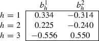
• Prices

  

• Utility values

  $$\begin{aligned} u_{1}\left( \mathbf {x}_{1}\right) =2.2473 \nonumber \\ u_{2}\left( \mathbf {x}_{2}\right) =2.4142 \nonumber \\ u_{3}\left( \mathbf {x}_{3}\right) =3.1676. \end{aligned}$$

  (25)

Above is the original equilibrium. Following planner intervention, we will obtain a new equilibrium. The planner intervenes according to:

$$\begin{aligned} \tau (1)= & {} 0 \\ \tau (2)= & {} -0.22 \\ \tau (3)= & {} 0 \\ \tau (4)= & {} -0.17. \end{aligned}$$

This means that the parameters $\widehat{\alpha }(1)$ and $\widehat{\alpha }(3)$ remain unchanged compared to $\alpha (1)$ and $\alpha (3),$ but $\widehat{\alpha }(2)$ is 22 % lower compared to $\alpha (2)$ and $\widehat{\alpha }(4)$ is 17 % lower compared to $\alpha (4)$:

$$\begin{aligned} \widehat{\alpha }(1)= & {} 0.033 \\ \widehat{\alpha }(2)= & {} 0.016 \\ \widehat{\alpha }(3)= & {} 0.029 \\ \widehat{\alpha }(4)= & {} 0.028\,. \end{aligned}$$

The credit constraints have just been tightened.

The equilibrium following planner intervention (again, unique²³) is:

• Consumption

  

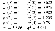
• Assets

  

• Prices

  

• Utility values

  $$\begin{aligned} u_{1}\left( \hat{\mathbf {x}}_{1}\right) =2.2603 \nonumber \\ u_{2}\left( \hat{\mathbf {x}}_{2}\right) =2.4259 \nonumber \\ u_{3}\left( \hat{\mathbf {x}}_{3}\right) =3.1686. \end{aligned}$$

  (26)

Comparing the utility values in (25) and (26), a Pareto improvement has been achieved. The utility increases are 0.58 % for household $h=1,$ 0.48 % for household $h=2,$ and 0.03 % for household $h=3.$

We now explain the intuition behind this Pareto improvement. Taken in isolation, a binding constraint of the form (7) for a single household $h$ and for a particular state $s\in \fancyscript{S}^{\prime }$ has well-established properties. A reduction in the parameter $\alpha _{h}(s)$ restricts the budget set for household $h,$ because the constraint has become tighter. This results in lower utility for household $h.$

However, consider what happens, as in the above example, when a reduction in the parameter $\alpha _{h}(s)$ results in constraints binding in some states in which they previously did not bind. Specifically, the following table illustrates this endogenous effect for the above example:

As can be seen from the table, for households $h=2$ and $h=3,$ different constraints are binding after the intervention compared to before the intervention. When the states of binding constraints  “switch” following an intervention, the property described above for isolated constraints is no longer valid. In particular, two effects now play a leading role in determining the equilibrium. First, portfolio effects are present as households adjust their portfolios across the states of uncertainty where now the constraints may bind for different states. Second, general equilibrium effects are present, whereby one household’s adjustments to the newly binding constraints must affect the other households, through the relative commodity prices and asset prices, in order for the market clearing conditions to be satisfied.

Appendix A

1.1 A.1: Proof of Theorem 13

The proof of Theorem 13 requires some preliminary results before proceeding.

Define $\varDelta _{+}^{G-1}=\big \{\mathbf {p}\in \mathbb {R}_{+}^{G}{:}\sum _{s=0}^{S}\sum _{c=1}^{C}p^{c}(s)=1\big \}$ and $\Pi ^{G-1}=\big \{\mathbf {p}\in \mathbb {R}^{G}{:}\sum _{s=0}^{S}\sum _{c=1}^{C}p^{c}(s)=1\big \}$.

In what follows, we take for given an economy $\left( \mathbf {e},\mathbf {u},\mathbf {y},\alpha \right)$.

From Proposition 12, we can define the following continuous functions.

$$\begin{aligned}&\mathbf {x}_{h}:\varDelta _{++}^{G-1}\times \fancyscript{G}_{A,S}\rightarrow \mathbb {R}^{G}, \quad \text {for }h\in \fancyscript{H}, \\&x_{1}\left( \mathbf {p},L\right) =\arg \max (20), \\&x_{h}\left( \mathbf {p},L\right) =\arg \max (18), \quad \text {for }\, h\in \fancyscript{H}\setminus \{1\}, \end{aligned}$$

and

$$\begin{aligned} z:\varDelta _{++}^{G-1}\times \fancyscript{G}_{A,S}\rightarrow \mathbb {R}^{G},\quad (\mathbf {p},L)\mapsto \sum _{h\in \fancyscript{H}}\left( x_{h}(\mathbf {p},L)-\mathbf {e}_{h}\right) . \end{aligned}$$

(27)

Define also

$$\begin{aligned} \psi :\varDelta _{+}^{G-1}\times \fancyscript{G}_{A,S}\rightarrow \mathbb {R}^{SA}, \quad \left( \mathbf {p},L\right) \mapsto \fancyscript{R}(\mathbf {p},\mathbf {y}). \end{aligned}$$

(28)

We say that a vector $\left( \mathbf {p}^{*},L^{*}\right)$ is a reduced Mr. 1 equilibrium for the economy $\bigl (\mathbf {e},\mathbf {u},\mathbf {y},\alpha \bigr )\in \fancyscript{E}$, if there exists $\mathbf {x}^{*}$ such that $\left( \mathbf {x}^{*},\mathbf {p}^{*},L^{*}\right)$ is a Mr. 1 equilibrium for that economy.

Proposition 16

A vector $\left( \mathbf {p}^{*},L^{*}\right)$ is a reduced Mr. $1$ equilibrium for the economy $\bigl (\mathbf {e},\mathbf {u},\mathbf {y},\alpha \bigr )\in \fancyscript{E}$ if

• 1. $z\left( \mathbf {p}^{*},L^{*}\right) =\mathbf {0}$ and

• 2. $\langle \psi \left( \mathbf {p}^{*},L^{*}\right) \rangle \subseteq L^{*}.$

In the next result we list some properties of the function $z$ in (27) we will need in the proof of Lemma 19.

Lemma 17

• 1. $z$ is continuous;

• 2. $z$ satisfies Walras’ law;

• 3. $z$ is bounded from below;

• 4. $z$ satisfies the boundary condition, i.e., if $(\mathbf {p}^{[n]},L^{[n]})\rightarrow (\bar{\mathbf {p}},\bar{L})$ with $\bar{\mathbf {p}}\in \partial \varDelta _{+}^{G-1},$ then $\Vert z(\mathbf {p}^{[n]},L^{[n]})\Vert \rightarrow \infty$.

Proof

• 1. It follows from Proposition 12.

• 2. It follows from household budget constraints.

• 3. From market clearing, for every $s,c,$ $z^{\,c}\left( s\right)$ is bounded below by $-\sum _{h\in \fancyscript{H}}{e}_{h}^{c}(s)$.

• 4. It follows from the budget constraint and the strict monotonicity of $u_{h.}$

In the proof of Theorem 13 we are going to use the following result in Husseini et al. (1990).

Theorem 18

(A Grassmannian Brouwer-like fixed point theorem) Let $H^{N}$ be an N-dimensional affine subspace, $C\subset H^{N}$ a compact convex subset with nonempty relative interior and let

$$\begin{aligned} \varPhi :C\times \fancyscript{G}_{A,S}\rightarrow H^{N},\quad \varPsi :C\times \fancyscript{G}_{A,S}\rightarrow \mathbb {R}^{AS} \end{aligned}$$

be continuous functions such that $\varPhi (\partial C,L)\subseteq C,\forall L\in \fancyscript{G}_{A,S}.$ Then there exists $(\bar{\mathbf {p}},\bar{L})$ such that

$$\begin{aligned} \varPhi (\bar{\mathbf {p}},\bar{L})=\bar{\mathbf {p}},\quad \langle \varPsi (\bar{\mathbf {p}},\bar{L})\rangle \subseteq \bar{L}. \end{aligned}$$

A crucial role in the application of the above theorem is played by the following lemma. We present the proof of the lemma in the case, analyzed in the present paper, in which the return space is described as a Grassmannian manifold. In fact, Husseini et al. (1990) presented instead the proof in the case of Stiefel manifolds.

Lemma 19

There exists a continuous function $\varphi :\varDelta _{+}^{G-1}\times \fancyscript{G}_{A,S}\rightarrow [0,1]$ such that the function

$\phi :\varDelta _{+}^{G-1}\times \fancyscript{G}_{A,S}\rightarrow \Pi ^{G-1}$ defined by

$$\begin{aligned} \phi (\mathbf {p},L)=\varphi (\mathbf {p},L) (p^{c}\left( s\right) +p^{c}\left( s\right) z^{c}\left( s\right) (\mathbf {p},L))_{s,c}+(1-\varphi (\mathbf {p},L))\mathbf {u}, \end{aligned}$$

(29)

where $\mathbf {u}=(\frac{1}{G},\dots ,\frac{1}{G})\in \mathbb {R}^{G},$ satisfies

• 1. $\phi (\partial \varDelta ^{G-1}_{+},L)\subseteq \varDelta ^{G-1}_{+},\,\forall L\in \fancyscript{G}_{A,S};$

• 2. $\phi (\mathbf {p},L)=\mathbf {p}\Leftrightarrow z(\mathbf {p},L)=\mathbf {0}.$ ²⁴

Proof

Define

$$\begin{aligned} V_{j}=\left\{ (\mathbf {p},L)\in \varDelta _{++}^{G-1}\times \fancyscript{G}_{A,S}:z_{j}(\mathbf {p},L)>0,\,p_{j}<\frac{1}{G}\right\} ,\quad j\in \{1,\dots ,G\} \end{aligned}$$

and $K=\left( \varDelta _{++}^{G-1}\times \fancyscript{G}_{A,S}\right) \setminus \left( \bigcup _{j=1}^{G}V_{j}\right) .$ We are going to prove that $K$ is closed in $\varDelta _{+}^{G-1}\times \fancyscript{G}_{A,S}.$ Since $\fancyscript{G}_{A,S}$ is a metric space, also $\varDelta _{+}^{G-1}\times \fancyscript{G}_{A,S}$ is a metric space. Thus it is enough to prove that $K$ is sequentially closed, i.e., that the limit point of any convergent sequence of elements of $K$ belongs to $K.$

Rewriting $K$ as follows

$$\begin{aligned} K=\left\{ (\mathbf {p},L)\in \varDelta _{++}^{G-1}\times \fancyscript{G}_{A,S}:\forall j\in \{1,\dots ,G\},\,z_{j}(\mathbf {p},L)\le 0 \text{ or } p_{j}\ge \frac{1}{G}\right\} \end{aligned}$$

and recalling that $\fancyscript{G}_{A,S}$ is compact, and thus closed, it is clear that the only way in which the limit point $(\bar{\mathbf {p}},\bar{L})$ of a sequence $(\mathbf {p}^{[n]},L^{[n]})$ of elements of $K$ does not belong to $K$ is that $\bar{\mathbf {p}}\in \partial \varDelta _{+}^{G-1}.$ However this is prevented by the boundary condition and the continuity of $z$ on $K.$ Indeed, if $\bar{\mathbf {p}}\in \partial \varDelta _{+}^{G-1},$ then there exists $j\in \{1,\dots ,G\}$ such that $\bar{p}_{j}=0.$ Hence there exists $\bar{n}\in \mathbb {N}$ such that, for every $n\ge \bar{n},$ $p_{j}^{[n]}<\frac{1}{G}.$ By definition of $K$ and recalling that $z$ is bounded from below, we then have $-\sum _{h\in \fancyscript{H}}e_{h}(j)\le z_{j}(\mathbf {p}^{[n]},L^{[n]})\le 0$ and thus, by the continuity of $z,$ it holds that $-\sum _{h\in \fancyscript{H}}e_{h}(j)\le z_{j}(\bar{\mathbf {p}},\bar{L})\le 0.$ On the other hand, by the boundary condition, $z_{j}(\mathbf {p}^{[n]},L^{[n]})\rightarrow +\infty .$ The contradiction is found.

Notice that $K\cap \left( \partial \varDelta _{+}^{G-1}\times \fancyscript{G} _{A,S}\right) =\varnothing$ and that $\partial \varDelta _{+}^{G-1}\times \fancyscript{G}_{A,S}$ is closed in $\varDelta _{+}^{G-1}\times \fancyscript{G}_{A,S}.$ Recalling that any metric space is normal²⁵ and that on normal spaces the Urysohn Lemma²⁶ applies, there exists a continuous function $\varphi :\varDelta _{+}^{G-1}\times \fancyscript{G}_{A,S}\rightarrow [0,1]$ such that $\varphi (K)=1$ and $\varphi (\partial \varDelta _{+}^{G-1}\times \fancyscript{G} _{A,S})=0.$ Let us then check that the function $\phi$ in (29) has $\Pi ^{G-1}$ as codomain and satisfies 1. and 2.

As regards the codomain of $\phi ,$ fix $(\mathbf {p},L)\in \varDelta _{+}^{G-1}\times \fancyscript{G}_{A,S}.$ Then $\sum _{j=1}^{G}p_{j}=1$ and recalling that $z$ obeys Walras’ law, it holds that

$$\begin{aligned}&\sum _{j=1}^{G}\phi _{j}(\mathbf {p},L)=\sum _{j=1}^{G}\left( \varphi (\mathbf {p},L)(p_{j}+p_{j}\,z_{j}(\mathbf {p},L))+(1-\varphi (\mathbf {p},L))\frac{1}{G}\right) \\&\quad =\varphi (\mathbf {p},L)\sum _{j=1}^{G}\left( p_{j}+p_{j}\,z_{j}(\mathbf {p},L)\right) +(1-\varphi (\mathbf {p},L))\sum _{j=1}^{G}\frac{1}{G}\\&\quad =\varphi (\mathbf {p},L)\sum _{j=1}^{G}p_{j}\,z_{j}(\mathbf {p},L)+1=1, \end{aligned}$$

i.e., $\phi (\varDelta _{+}^{G-1}\times \fancyscript{G}_{A,S})\subseteq \Pi ^{G-1},$ as desired.

In regard to 1., as we already know that $\phi (\partial \varDelta _{+}^{G-1}\times \fancyscript{G}_{A,S})\subseteq \Pi ^{G-1},$ in order to show that $\phi (\partial \varDelta _{+}^{G-1}\times \fancyscript{G}_{A,S})\subseteq \varDelta _{+}^{G-1},$ it is enough to check that $\phi _{j}(\mathbf {p},L)\ge 0,$ for every $(\mathbf {p},L)\in \partial \varDelta _{+}^{G-1}\times \fancyscript{G}_{A,S}$ and $j\in \{1,\dots ,G\}.$ Since $\varphi (\partial \varDelta _{+}^{G-1}\times \fancyscript{G}_{A,S})=0,$ it holds that, for $(\mathbf {p},L)\in \partial \varDelta _{+}^{G-1}\times \fancyscript{G}_{A,S},$ $\phi _{j}(\mathbf {p},L)=\frac{1}{G}\ge 0.$

Let us finally prove 2. Assume that $z(\mathbf {p},L)=\mathbf {0}$ and show that $\phi (\mathbf {p},L)=\mathbf {p}.$ If $z(\mathbf {p},L)=\mathbf {0}$ then $z_{j}(\mathbf {p},L)\le 0$ for every $j$ and so $(\mathbf {p},L)\in K.$ Hence, $\varphi (\mathbf {p},L)=1$ and thus $\phi _{j}(\mathbf {p},L)=p_{j}+p_{j}\,z_{j}(\mathbf {p},L)=p_{j},$ for every $j,$ as desired.

Assume now that $\phi (\mathbf {p},L)=\mathbf {p}$ and show that $z(\mathbf {p},L)=\mathbf {0}.$ Notice that

$$\begin{aligned} \varDelta _{+}^{G-1}\times \fancyscript{G}_{A,S}=\left( \partial \varDelta _{+}^{G-1}\times \fancyscript{G}_{A,S}\right) \cup K\cup \left( \bigcup _{j=1}^{G}V_{j}\right) \end{aligned}$$

and that $\partial \varDelta _{+}^{G-1}\times \fancyscript{G}_{A,S},K$ and $\bigcup _{j=1}^{G}V_{j}$ are pairwise disjoint. If $(\mathbf {p},L)\in \varDelta _{+}^{G-1}\times \fancyscript{G}_{A,S},$ then there are three cases to consider, i.e., $(\mathbf {p},L)\in \partial \varDelta _{+}^{G-1}\times \fancyscript{G}_{A,S},$ $(\mathbf {p},L)\in K$ and $(\mathbf {p},L)\in V_{j^{*}},$ for some $j^{*}\in \{1,\dots ,G\}.$ We claim that only in the second case it may happen that $\phi (\mathbf {p},L)=\mathbf {p}.$ Indeed, in the first case $\phi (\mathbf {p},L)=\left( \frac{1}{G} ,\dots ,\frac{1}{G}\right) \notin \partial \varDelta _{+}^{G-1}.$ In the third case, by definition of $V_{j^{*}},$ we would have

$$\begin{aligned} p_{j^{*}}= & {} \phi _{j^{*}}(\mathbf {p},L)=\varphi (\mathbf {p},L)(p_{j^{*}}+p_{j^{*}}\,z({j^{*}})(\mathbf {p},L))+(1-\varphi (\mathbf {p},L))\frac{1}{G}\\> & {} \varphi (\!\mathbf {p},L)(p_{j^{*}}+p_{j^{*}}\,z({j^{*}})(\!\mathbf {p},L))+(1-\varphi (\!\mathbf {p},L))p_{j^{*}}\\= & {} p_{j^{*}}+\varphi (\!\mathbf {p},L)p_{j^{*}}\,z({j^{*}})(\!\mathbf {p},L)\ge p_{j^{*}}, \end{aligned}$$

a contradiction. Thus $\phi (\mathbf {p},L)=\mathbf {p}$ only if $(\mathbf {p},L)\in K$ and in this case, as $\varphi (\mathbf {p},L)=1,$ it follows that, for every $j\in \{1,\dots ,G\},$ $p_{j}=\phi _{j}(\mathbf {p},L)=p_{j}+p_{j}\,z_{j}(\mathbf {p},L),$ from which, since $p_{j}>0,$ we have $z_{j}(\mathbf {p},L)=0,$ as desired.

Proof of Theorem 13

We want to apply Theorem 18, identifying $\varPhi$ and $\varPsi$ with $\phi$ in (29) and $\psi$ in (28), respectively. $\Pi ^{G-1}$ is an affine subspace of $\mathbb {R}^{G}$ and $\varDelta _{+}^{G-1}\subset \Pi ^{G-1}$ is clearly a compact, convex subset with nonempty relative interior. $\phi$ is a continuous function from Lemma 17 and from the fact that $\varphi$ is a continuous function from Lemma 19. Again from the latter lemma, we have that $\phi (\partial \varDelta _{+}^{G-1},L)\subseteq \varDelta _{+}^{G-1},\,\forall L\in \fancyscript{G}_{A,S}$. Finally, from Theorem 18 and Proposition 16, the desired result follows. $\square$

1.2 A.2: Proof of Theorem 14

Let $\fancyscript{V}$ be a topological Hausdorff vector space, $V\subseteq \fancyscript{V}$ be an open set and $f:V\rightarrow \mathbb {R}^{n}$ be a function. We say that $f\in C^{0}(V,\mathbb {R}^{n})$ if $f$ is continuous, while $f\in C^{1}(V,\mathbb {R}^{n})$ if it is continuous, there exists the limit

$$\begin{aligned} df(\mathbf {v},\mathbf {w})=\lim _{\varepsilon \rightarrow 0}\frac{f(\mathbf {v}+\varepsilon \mathbf {w})-f(\mathbf {v})}{\varepsilon } ,\quad \forall \mathbf {v}\in V,\mathbf {w}\in \fancyscript{V}, \end{aligned}$$

and the function $df:V\times \fancyscript{V}\rightarrow \mathbb {R}^{n}$ is continuous.

Given any (not necessarily open) set $X\subseteq \fancyscript{V}$ and $f:X\rightarrow \mathbb {R}^{n}$, we say $f\in C^{0}(X,\mathbb {R}^{n})$ if $f$ is continuous with respect to the topology induced by $\fancyscript{V}$ on $X$, while, as in the finite dimensional setting, $f\in C^{1}(X,\mathbb {R}^{n})$ if for every $\mathbf {v_{0}}\in X$ there exists an open neighborhood of $\mathbf {v_{0}}$ in $\fancyscript{V}$, say $V(\mathbf {v_{0}})$, and a function $\overline{f}:V(\mathbf {v_{0}})\rightarrow \mathbb {R}^{n}$ such that $\overline{f}\in C^{1}(V(\mathbf {v_{0}}),\mathbb {R}^{n})$ and, for every $\mathbf {x}\in V(\mathbf {v_{0}})\cap X,\,f(\mathbf {x})=\overline{f}(\mathbf {x}).$

Those definitions allow to state the following implicit function theorem which is a simplified version of Theorem 2.3 in Glöckner (2006).²⁷

Theorem 20

Let us consider $f{:}O\times V\rightarrow \mathbb {R}^{n}$, where $O$ is an open subset of $\mathbb {R}^{n}$ and $V$ is an open subset of a topological Hausdorff vector space $\fancyscript{V}$. Assume $f\in C^{1}(O\times V,\mathbb {R}^{n})$ and let $(\mathbf {x_{0}},\mathbf {v_{0}})\in O\times V$ such that $f(\mathbf {x_{0}},\mathbf {v_{0}})=\mathbf {0}$ and $\mathbf {D_{x}f}(\mathbf {x_0},\mathbf {v_0})$ is invertible.²⁸ Then there exist $O(\mathbf {x_{0}})\subseteq O$ open neighborhood of $\mathbf {x_{0}}$, $V(\mathbf {v_{0}})\subseteq V$ open neighborhood of $\mathbf {v_{0}}$ and $g{:}V(\mathbf {v_{0}})\rightarrow O(\mathbf {x_{0}})$ such that

• 1. $g\in C^{1}(V(\mathbf {v_{0}}),O(\mathbf {x_{0}}))$,

• 2. $g(\mathbf {v_{0}})=\mathbf {x_{0}}$,

• 3. $\{(\mathbf {x},\mathbf {v})\in O(\mathbf {x_{0}})\times V(\mathbf {v_{0}}):f(\mathbf {x},\mathbf {v})=\mathbf {0}\}=\{(\mathbf {x},\mathbf {v})\in O(\mathbf {x_{0}})\times V(\mathbf {v_{0}}):\mathbf {x}=g(\mathbf {v})\}$.

Proof of Theorem 14

Step 1.

Define, for each $\sigma \in \Sigma ,$

$$\begin{aligned} \varXi _{\sigma }=\mathbb {R}_{++}^{GH}\times \mathbb {R}^{(S+1)H}\times \mathbb {R }^{AH}\times \mathbb {R}^{SH}\times \mathbb {R}_{++}^{G}\times \mathbb {R}^{A}\times V_{{\sigma }^{-1} }, \end{aligned}$$

(30)

with generic element

$$\begin{aligned} \xi =\left( \left( \mathbf {x}_{h},\lambda _{h},\mathbf {b}_{h},\mu _{h}\right) _{h\in \fancyscript{H}},\mathbf {p},\mathbf {q},L\right) =\left( \mathbf {x},\lambda ,\mathbf {b},\mu ,\mathbf {p},\mathbf {q},L\right) , \end{aligned}$$

and the function

$$\begin{aligned} \fancyscript{F}_{\sigma }:\varXi _{\sigma }\times \fancyscript{E}\rightarrow \mathbb {R}^{\dim (\varXi _{\sigma })}, \end{aligned}$$

$$\begin{aligned} \fancyscript{F}_{\sigma }\left( \xi ,\mathbf {e},\mathbf {u},\mathbf {y},\alpha \right) ={\left[ \begin{array}{ll}&\begin{array}{l} \mathbf {D_{x_{h}(s)}u}_{h}(\mathbf {x}_{h})-\lambda _{h}(s)\mathbf {p}(s) \end{array}\\ &{} \begin{array}{l} -\varPhi \left( \mathbf {p}\right) \left( \mathbf {x}_{h}-\mathbf {e}_{h}\right) +\left[ \begin{array}{l} -\mathbf {q} \\ \mathbf {P}_{\sigma }\left[ \begin{array}{l} -\psi (L) \\ \mathbf {I}_{A} \end{array} \right] \end{array} \right] \mathbf {b_{h}} \end{array} \\ &{} \lambda _{h}\left[ \begin{array}{l} -\mathbf {q} \\ \mathbf {P}_{\sigma }\left[ \begin{array}{l} -\psi (L) \\ \mathbf {I}_{A} \end{array} \right] \end{array} \right] +\mu _{h}\mathbf {P}_{\sigma }\left[ \begin{array}{l} -\psi (L) \\ \mathbf {I}_{A} \end{array} \right] \\ &{} \begin{array}{l} \min \left\{ \mu _{h},\mathbf {P}_{\sigma }\left[ \begin{array}{l} -\psi (L) \\ \mathbf {I}_{A} \end{array} \right] \mathbf {b}_{h}+\mathbf {A}_{h}\varPhi ^{\mathbf {1}}\left( \mathbf {p}\right) \mathbf {e}_{h}^{\mathbf {1}}\right\} \end{array} \\ &{} \begin{array}{l} \underset{h=1}{\overset{H}{\sum }}\big (\mathbf {x}_{h}^{\backslash }-\mathbf {e}_{h}^{\backslash }\big ) \end{array} \\ &{} \begin{array}{l} \underset{h=1}{\overset{H}{\sum }}\mathbf {b}_{h} \end{array} \\ &{} \begin{array}{l} p^{1}(s)-1 \end{array}\\ &{} \begin{array}{l} \mathrm {vec}\left[ \mathbf {I}_{S-A}\ |\ \psi \left( L\right) \right] \cdot \mathbf {P}_{\sigma ^{-1}}\cdot \fancyscript{R}\left( \mathbf {p},\mathbf {y}\right) \end{array} \end{array} \right] } \end{aligned}$$

(31)

where $\psi :V_{{\sigma }^{-1} }\rightarrow \mathbb M(S-A,A)$ is the diffeomorphism in (15), with $V_{{\sigma }^{-1} }\subseteq \fancyscript{G}_{A,S}$ open.

For simplicity and without loss of generality, from now on we consider the case $\mathbf {P}_{\sigma } =\mathbf {I},$ so that $\fancyscript{F}_{\sigma }$ becomes $\fancyscript{F}:\varXi \times \fancyscript{E}\rightarrow \mathbb R^{\dim (\varXi )}.$

We now show that border line cases are rare. For every $h\in \fancyscript{H},$ we define $\fancyscript{S}_{h}^{1},\fancyscript{S}_{h}^{2}$ and $\widehat{\fancyscript{S}}_{h}^{1}$ so that $\left\{ 1,\dots ,S\right\} =\fancyscript{S}_{h}^{1}\cup \fancyscript{S}_{h}^{2}$, with $\left( \fancyscript{S}_{h}^{1}\setminus \widehat{\fancyscript{S}}_{h}^{1}\right) \cap \fancyscript{S}_{h}^{2}=\varnothing$ and $\widehat{\fancyscript{S}}_{h}^{1}\subseteq \fancyscript{S}_{h}^{1},$ in order to have

where we have denoted by $\mathbf {m}(s)$ the $s$-th row of $\left[ \begin{array}{l} -\psi (L) \\ \mathbf {I}_{A} \end{array} \right]$.

Define $\hat{\mathbf {y}}=(y^{a,1}(s))_{a\in \fancyscript{A},\,s\in \{1,\dots ,S-A\}}$ and the full rank matrix

$$\begin{aligned} \mathbf {B}={\left[ \begin{array}{lllllll} {p}^{1}(1) &{} &{} &{} &{} &{} &{} \\ &{} \ddots &{} &{} &{} &{} &{} \\ &{} &{} p^{1}(1) &{} &{} &{} &{} \\ &{} &{} &{} \ddots &{} &{} &{} \\ &{} &{} &{} &{} p^{1}(S-A) &{} &{} \\ &{} &{} &{} &{} &{} \ddots &{} \\ &{} &{} &{} &{} &{} &{} p^{1}(S-A) \\ \end{array} \right] .} \end{aligned}$$

The computation of the desired (partial) Jacobian matrix is presented in the table below, where the following conventions are adopted.

• (a) The symbol $\circledcirc$ denotes a matrix which is insignificant for our argument, while no symbol means $0.$ For size convenience, just in the table below, we set

  $$\begin{aligned} \mathbf {R}\left( \mathbf {q}\right) =\left[ \begin{array}{l} -\mathbf {q} \\ -\psi (L) \\ \mathbf {I} \end{array}\right] \quad \text{ and } \quad \mathbf {R}=\left[ \begin{array}{l} -\psi (L) \\ \mathbf {I} \end{array} \right] . \end{aligned}$$

• (b) The $*$ next to a matrix indicates that it is a full row rank matrix.

• (c) The desired full rank result is obtained as follows. In each super-row, use the starred matrix to clean up that super-row, being sure that in that super-column there are only zero matrices. An order in which the appropriate elementary (super) column operations have to be performed is the one indicated in the last column of the table.

where, for $h\in \fancyscript{H},$ we have set $\mathbf {Z}_{h}^{1}$ equal to the square diagonal matrix with elements $\mathbf {p}(s)\mathbf {e}_{h}(s),$ for $s\in \fancyscript{S}_{h}^{1},$ on the diagonal. Moreover

$$\begin{aligned} \varPhi \bigl ( \mathbf {p^{1}}\bigr ) =\left[ \begin{array}{llll} p^{1}\left( 0\right) &{} &{} &{} \\ &{} p^{1}\left( 1\right) &{} &{} \\ &{} &{} \ddots &{} \\ &{} &{} &{} p^{1}\left( S\right) \end{array} \right] . \end{aligned}$$

Step 2.

After having shown that border line cases are rare, we are going to prove that in a full measure subset of $\mathbb R_{++}^{GH}\times \mathbb R^{CAS},$ the return matrix $\fancyscript{R}(\mathbf {p},\mathbf {y})$ has full rank. Actually, we are going to show that its square $A$-dimensional submatrix $\widehat{\fancyscript{R}}(\mathbf {p},\mathbf {y})$ has full rank, where

$$\begin{aligned}&\widehat{\fancyscript{R}}(\!\mathbf {p},\mathbf {y})\\&\quad ={\left[ \begin{array}{lllll} \mathbf {p}(S-A+1)\mathbf {y}^{1}(S-A+1) &{} \cdots &{} \mathbf {p}(S-A+1)\mathbf {y}^{a}(S-A+1) &{} \cdots &{} \mathbf {p}(S-A+1)\mathbf {y}^{A}(S-A+1) \\ \vdots &{} &{} \vdots &{} &{} \vdots \\ \mathbf {p}(S-A+a)\mathbf {y}^{1}(S-A+a) &{} \ldots &{} \mathbf {p}(S-A+a)\mathbf {y}^{a}(S-A+a) &{} \ldots &{} \mathbf {p}(S-A+a)\mathbf {y}^{A}(S-A+a) \\ \vdots &{} &{} \vdots &{} &{} \vdots \\ \mathbf {p}(S)\mathbf {y}^{1}(S) &{} \ldots &{} \mathbf {p}(S)\mathbf {y}^{a}(S) &{} \ldots &{} \mathbf {p}(S)\mathbf {y}^{A}(S) \end{array} \right] }, \end{aligned}$$

by showing that $\varvec{0}$ is a regular value for $(F,G):\varXi \times \fancyscript{E}\times \mathbb R^{A}\rightarrow \mathbb R^{\dim (\varXi )+(A+1)},$ where

$$\begin{aligned} G:\varXi \times \fancyscript{E}\times \mathbb {R}^{A}\rightarrow \mathbb {R}^{A+1},\quad (\xi ,\mathbf {e},\mathbf {u},\mathbf {y},\alpha ,\mathbf {d})\mapsto (\mathbf {d}\cdot \widehat{\fancyscript{R}}(\mathbf {p},\mathbf {y}),\mathbf {d}\mathbf {d}-1). \end{aligned}$$

Calling $\mathbf {T}$ the Jacobian matrix in the previous page, we then have to show that the following matrix

$$\begin{aligned} { \left[ \begin{array}{l@{\quad }l@{\quad }l} \mathbf {T} &{} \star &{} \mathbf {0} \\ \mathbf {0} &{} \mathbf {N} &{} \widehat{\fancyscript{R}}(\mathbf {p},\mathbf {y}) \\ \mathbf {0} &{} \mathbf {0} &{} 2\mathbf {d}^{T} \end{array}\!\right] } \end{aligned}$$

has full rank, where the last two columns are the derivatives with respect to  $\widehat{\!\widehat{\mathbf {y}}}$ and $\mathbf {d},$ respectively, with   $\widehat{\!\widehat{\mathbf {y}}}$ defined hereinafter.

As $\mathbf {d}=(d(S-A+a))_{a\in \fancyscript{A}}$ is such that $\mathbf {d}\mathbf {d}=1,$ then there exists $\bar{a}\in \fancyscript{A}$ such that $d(S-A+\bar{a})\ne 0.$ Then we set  $\widehat{\!\widehat{\mathbf {y}}}=\left( y^{a,1}(S-A+\bar{a})\right) _{a\in \fancyscript{A} }\in \mathbb {R}^{A}.$ Notice that

$$\begin{aligned} \mathbf {d}\cdot {\widehat{\fancyscript{R}}}(\mathbf {p},\mathbf {y})={\left[ \begin{array}{c} \sum _{j=1}^{A}d(S-A+j)\mathbf {p}(S-A+j)\mathbf {y}^{1}(S-A+j) \\ \vdots \\ \sum _{j=1}^{A}d(S-A+j)\mathbf {p}(S-A+j)\mathbf {y}^{a}(S-A+j) \\ \vdots \\ \sum _{j=1}^{A}d(S-A+j)\mathbf {p}(S-A+j)\mathbf {y}^{A}(S-A+j) \end{array} \right] } \end{aligned}$$

and thus

$$\begin{aligned}&\mathbf {N} \\&\quad ={\left[ \begin{array}{lllll} d(S-A+\bar{a})p^{1}(S-A+\bar{a}) &{} &{} &{} &{} \\ &{} \ddots &{} &{} &{} \\ &{} &{} d(S-A+\bar{a})p^{1}(S-A+\bar{a}) &{} &{} \\ &{} &{} &{} \ddots &{} \\ &{} &{} &{} &{} d(S-A+\bar{a})p^{1}(S-A+\bar{a}) \\ \end{array} \right] } \end{aligned}$$

which has clearly full rank. This concludes the proof of the step.

Step 3.

The proof is given in Proposition 21 below.

Step 4.

Apply Theorem 20. $\square$

Recalling the definition of $\varXi _{\sigma }$ in (30), we rewrite the function $\fancyscript{F}_{\sigma }:\varXi _{\sigma }\times \fancyscript{E}\rightarrow \mathbb {R}^{\dim (\varXi _{\sigma })}$ in (31) as

$$\begin{aligned}&\fancyscript{F}_{\sigma }\left( \xi ,\mathbf {e},\mathbf {u},\mathbf {y},\alpha \right) \\&\quad ={\left[ \begin{array}{ll}&\begin{array}{l} \mathbf {D_{x_{h}(s)}u}_{h}(\mathbf {x}_{h})-\lambda _{h}(s)\mathbf {p}(s) \end{array} \\ &{} \begin{array}{l} -{\mathbf {p}}(0)(\mathbf {x}_{h}(0)-\mathbf {e}_{h}(0))-\mathbf {q}\mathbf {b}_{h} \\ -{\mathbf {p}}(s)(\mathbf {x}_{h}(s)-\mathbf {e}_{h}(s))-\underset{a=1}{\overset{A}{\sum }}m_{\sigma ^{-1}(s)a}b_{h}^{a},\quad \sigma ^{-1}(s)\in \{1,\ldots ,S-A\} \\ -{\mathbf {p}}(s)(\mathbf {x}_{h}(s)-\mathbf {e}_{h}(s))+b_{h}^{\sigma ^{-1}(s)-(S-A)},\quad \sigma ^{-1}(s)\in \{S-A+1,\ldots ,S\} \end{array} \\ &{} \begin{array}{l} -\lambda _{h}(0)q^{\sigma ^{-1}(s)-(S-A)}-\underset{\sigma ^{-1}(s)=1}{ \overset{S-A}{\sum }}(\lambda _{h}(s)+\mu _{h}(s))m_{\sigma ^{-1}(s)(\sigma ^{-1}(s)-(S-A))}+ \\ +\lambda _{h}(s)+\mu _{h}(s),\quad \sigma ^{-1}(s)\in \{S-A+1,\ldots ,S\} \end{array} \\ &{} \begin{array}{l} \min \left\{ \mu _{h},\mathbf {P}_{\sigma }\left[ \begin{array}{l} -\psi (L) \\ \mathbf {I}_{A} \end{array} \right] \mathbf {b}_{h}+\mathbf {A}_{h}\varPhi ^{\mathbf {1}}\left( \mathbf {p}\right) \mathbf {e}_{h}^{\mathbf {1}}\right\} \end{array} \\ &{} \begin{array}{l} \underset{h=1}{\overset{H}{\sum }}\big (\mathbf {x}_{h}^{\backslash }-\mathbf {e}_{h}^{\backslash }\big ) \end{array} \\ &{} \begin{array}{l} \underset{h=1}{\overset{H}{\sum }}\mathbf {b}_{h} \end{array} \\ &{} \begin{array}{l} p^{1}(s)-1 \end{array} \\ &{} \begin{array}{l} \mathrm {vec}\left[ \mathbf {I}_{S-A}\ |\ \psi \left( L\right) \right] \cdot \mathbf {P}_{\sigma ^{-1}}\cdot \fancyscript{R}\left( \mathbf {p},\mathbf {y}\right) \end{array} \end{array} \right] } \end{aligned}$$

where $L\in V_{{\sigma }^{-1} }$ and $\psi (L)=(m_{sa})_{s\in \left\{ 1,\dots ,S-A\right\} ,\,a\in \fancyscript{A}}\in \mathbb M(S-A,A).$

We also recall that a function $f:A\rightarrow B,$ with $A$ and $B$ topological spaces, is proper if, for every $K\subseteq B$ compact set, $f^{-1}(K)\subseteq A$ is compact as well. We also recall that any proper and continuous function is closed, i.e., it maps closed sets onto closed sets.

Proposition 21

$\fancyscript{F}_{\sigma }$ is continuous on $\varXi _{\sigma }\times \fancyscript{E}$ and

$$\begin{aligned} \pi :\bigcup _{\sigma \in \Sigma }\fancyscript{F}_{\sigma }^{-1}(\mathbf {0})\rightarrow \fancyscript{E},\quad \left( \xi ,\mathbf {e},\mathbf {u},\mathbf {y},\alpha \right) \mapsto \pi \left( \xi ,\mathbf {e},\mathbf {u},\mathbf {y},\alpha \right) =(\mathbf {e},\mathbf {u},\mathbf {y},\alpha ) \end{aligned}$$

is proper.

Proof

The continuity of $\fancyscript{F}_{\sigma }$ is immediate. In order to show that $\pi$ is proper, we have to prove that each sequence $(\xi ^{[n]},\mathbf {e}^{[n]},\mathbf {u}^{[n]},\mathbf {y}^{[n]},\alpha ^{[n]})_{n\in \mathbb {N}}$ in $\bigcup _{\sigma \in \Sigma }\fancyscript{F}_{\sigma }^{-1}(\mathbf {0}),$ such that $(\mathbf {e}^{[n]},\mathbf {u}^{[n]},\!\mathbf {y}^{[n]},\!\alpha ^{[n]}\!)$ converges in $\fancyscript{E}$, admits a converging subsequence in $\bigcup _{\sigma \in \Sigma }\fancyscript{F}_{\sigma }^{-1}(\mathbf {0}).$ Since $\fancyscript{G}_{A,S}$ is sequentially compact, let us assume that

$$\begin{aligned} (\mathbf {e}^{[n]},\mathbf {u}^{[n]},\mathbf {y}^{[n]},\alpha ^{[n]},L^{[n]})\rightarrow (\overline{ \mathbf {e}},\overline{\mathbf {u}},\overline{\mathbf {y}},\overline{\alpha },\overline{L})\in \fancyscript{E} \times \fancyscript{G}_{A,S}. \end{aligned}$$

Therefore there exists $\sigma \in \Sigma$ such that $\overline{L}\in V_{{\sigma }^{-1} }$ and for sufficiently large $n,$ $L^{[n]}\in V_{{\sigma }^{-1} },$ too. Without loss of generality we can assume that $\mathbf {P}_{\sigma }=\mathbf {I}$, so that $\fancyscript{F}_{\sigma }$ simply becomes

$$\begin{aligned}&\!\!\! \fancyscript{F}\left( \xi ,\mathbf {e},\mathbf {u},\mathbf {y},\alpha \right) \nonumber \\&\!\!\! \quad ={\left[ \begin{array}{ll} (\mathrm{32a})&\quad \begin{array}{l} \mathbf {D_{x_{h}(s)}u}_{h}(\mathbf {x}_{h})-\lambda _{h}(s)\mathbf {p}(s)\end{array}\\ (\mathrm{32b}) &{}\quad \begin{array}{l} -{\mathbf {p}}(0)(\mathbf {x}_{h}(0)-\mathbf {e}_{h}(0))-\mathbf {q}\mathbf {b}_{h} \\ -{\mathbf {p}}(s)(\mathbf {x}_{h}(s)-\mathbf {e}_{h}(s))-\underset{a=1}{\overset{A}{\sum }} m_{sa}b_{h}^{a},\quad s\in \{1,\ldots ,S-A\} \\ -{\mathbf {p}}(s)(\mathbf {x}_{h}(s)-\mathbf {e}_{h}(s))+b_{h}^{s-(S-A)},\quad s\in \{S-A+1,\ldots ,S\}\end{array}\\ (\mathrm{32c}) &{}\quad \begin{array}{l} -\lambda _{h}(0)q^{a}-\underset{s=1}{\overset{S-A}{\sum }}(\lambda _{h}(s)+\mu _{h}(s))m_{sa}+\lambda _{h}(S-A+a)+\mu _{h}(S-A+a) \\ \end{array} \\ (\mathrm{32d}) &{}\quad \begin{array}{l} \min \left\{ \mu _{h},\left[ \begin{array}{l} -\psi (L) \\ \mathbf {I}_{A} \end{array} \right] \mathbf {b}_{h}+\mathbf {A}_{h}\varPhi ^{\mathbf {1}}\left( \mathbf {p}\right) e_{h}^{\mathbf {1}}\right\} \end{array} \\ (\mathrm{32e}) &{}\quad \begin{array}{l} \underset{h=1}{\overset{H}{\sum }}\big (\mathbf {x}_{h}^{\backslash }-\mathbf {e}_{h}^{\backslash }\big ) \end{array} \\ (\mathrm{32f}) &{}\quad \begin{array}{l} \underset{h=1}{\overset{H}{\sum }}\mathbf {b}_{h} \end{array} \\ (\mathrm{32g}) &{}\quad \begin{array}{l} p^{1}(s)-1 \end{array} \\ (\mathrm{32h}) &{}\quad \begin{array}{l} \mathrm {vec}\left[ \mathbf {I}_{S-A}\ |\ \psi \left( L\right) \right] \cdot \fancyscript{R}\left( \mathbf {p},\mathbf {y}\right) \end{array} \end{array} \!\!\!\right] }\nonumber \\ \end{aligned}$$

(32)

Then it suffices to show that, up to a subsequence, $(\xi ^{[n]})_{n\in \mathbb {N}}$ converges to a certain $\overline{\xi }\in \varXi :$ indeed the condition $\fancyscript{F}(\overline{\xi },\overline{\mathbf {e}},\overline{\mathbf {u}},\overline{\mathbf {y}},\overline{\alpha })=\mathbf {0}$ follows by the continuity of $\fancyscript{F}.$ As we are going to use a diagonal argument, every time we say that a sequence converges we mean it has a converging subsequence. Let us start with the convergence of $\mathbf {x}^{[n]}.$ For a fixed $h\in \fancyscript{H},$ we know that, for every $n\in \mathbb N,\,\bigl (\mathbf {x}_{h}^{[n]},\mathbf {b}_{h}^{[n]}\bigr )$ is solution to the problem

$$\begin{aligned}&\underset{(\mathbf {x}_{h},\mathbf {b}_{h})}{\max }\,u_{h}^{[n]}\left( \mathbf {x}_{h}\right) \nonumber \\&s.t. -\mathbf {p}^{[n]}\left( 0\right) \left( \mathbf {x}_{h}\left( 0\right) -\mathbf {e}_{h}^{[n]}\left( 0\right) \right) -\mathbf {q}^{[n]}\mathbf {b}_{h}=0 \end{aligned}$$

(33)

$$\begin{aligned}&-\varPhi ^{\mathbf {1}}\bigl ( \mathbf {p}^{[n]}\bigr ) \left( \mathbf {x}_{h}^{\mathbf {1}}-\mathbf {e}_{h}^{[n]\mathbf {1}}\right) +\left[ \begin{array}{l} -\psi (L^{[n]}) \\ \mathbf {I}_{A} \end{array} \right] \mathbf {b}_{h}=\mathbf {0} \end{aligned}$$

(34)

$$\begin{aligned}&\left[ \begin{array}{l} -\psi (L^{[n]}) \\ \mathbf {I}_{A} \end{array} \right] \mathbf {b}_{h}+\mathbf {A}_{h}^{[n]}\varPhi ^{\mathbf {1}}\bigl ( \mathbf {p}^{[n]}\bigr ) \mathbf {e}_{h}^{[n]\mathbf {1}}\ge \mathbf {0} \end{aligned}$$

(35)

and then, since $(\mathbf {e}_{h}^{[n]},\mathbf {0})$ belongs to the constraint set, it has to be $u_{h}^{[n]}(\mathbf {x}_{h}^{[n]})\ge u_{h}^{[n]}(\mathbf {e}_{h}^{[n]})$. Since $(\mathbf {e}_{h}^{[n]})_{n\in \mathbb {N}}$ converges to $\overline{\mathbf {e}}_{h}\in \mathbb R_{++}^{G},$ it holds that the compact set $E_{h}=\bigl \{\mathbf {e}_{h}^{[n]}\bigr \}_{n\in \mathbb {N}}\cup \{\overline{\mathbf {e}}_{h}\}$ is a subset of $\mathbb R_{++}^{G}$ and we have

$$\begin{aligned} u_{h}^{[n]}(\mathbf {x}_{h}^{[n]})\ge u_{h}^{[n]}(\mathbf {e}_{h}^{[n]})\ge \min _{\mathbf {x}_{h}\in E_{h}}u_{h}^{[n]}(\mathbf {x}_{h})\ge \min _{\mathbf {x}_{h}\in E_{h}}\overline{u}_{h}(\mathbf {x}_{h})-\varepsilon ^{[n]}, \end{aligned}$$

for a suitable sequence $(\varepsilon ^{[n]})_{n\in \mathbb {N}}$ in $\mathbb R_{++}$ such that $\varepsilon ^{[n]}\rightarrow 0$ if $n\rightarrow \infty ,$ by the definition of the topology on $C^{2}(\mathbb R_{++}^{G}).$ Indeed we can define, for every $n\in \mathbb N,$

$$\begin{aligned} \varepsilon ^{[n]}=\max _{\mathbf {w}\in E_{h}}\big \vert u_{h}^{[n]}\left( \mathbf {w}\right) -\overline{u}_{h}\left( \mathbf {w}\right) \big \vert . \end{aligned}$$

Let $\mathbf {x}_{h}^{*}\in E_{h}$ be such that $\min _{\mathbf {x}_{h}\in E_{h}}\overline{u}_{h}(\mathbf {x}_{h})=\overline{u}_{h}(\mathbf {x}_{h}^{*}),$ and let $\mathbf {1}=(1,\ldots ,1)\in \mathbb R^{G}$ and $\delta >0$ be small enough such that $\mathbf {x}_{h}^{*}-2\delta \mathbf {1}\in \mathbb R_{++}^{G}.$ Obviously, since by (3), $\overline{u}_{h}(\mathbf {x}_{h}^{*})>\overline{u}_{h}(\mathbf {x}_{h}^{*}-\delta \mathbf {1})$, there exists $n_{1}$ such that $n\ge n_{1}$ implies $\overline{u}_{h}(\mathbf {x}_{h}^{*})-\varepsilon ^{[n]}\ge \overline{u}_{h}(\mathbf {x}_{h}^{*}-\delta \mathbf {1})$ and thus, for every $n\ge n_{1},$

$$\begin{aligned} u_{h}^{[n]}(\mathbf {x}_{h}^{[n]})\ge \overline{u}_{h}(\mathbf {x}_{h}^{*}-\delta \mathbf {1}). \end{aligned}$$

(36)

Of course, because of the validity of $S+1$ Walras’ laws in our model, we can also assume that, for every $n\ge n_{1},$

$$\begin{aligned} \mathbf {0}\ll \mathbf {x}_{h}^{[n]}\le \sum _{h=1}^{H}\mathbf {e}_{h}^{[n]}\le \sum _{h=1}^{H}\overline{\mathbf {e}}_{h}+\mathbf {1}. \end{aligned}$$

Our purpose now is to prove that for infinite values of $n$ it is $\overline{ u}_{h}(\mathbf {x}_{h}^{[n]})\ge \overline{u}_{h}(\mathbf {x}_{h}^{*}-2\delta \mathbf {1}).$ Let $\widehat{\mathbf {x}}_{h}\in \big [\mathbf {0},\sum _{h=1}^{H}\overline{\mathbf {e}}_h+\mathbf {1}\big ]$ be a cluster point of $(\mathbf {x}_{h}^{[n]})_{n\ge n_{1}}.$ Then we can assume $\mathbf {x}_{h}^{[n]}\rightarrow \widehat{\mathbf {x}}_{h}.$ Consider any $\widetilde{\mathbf {x}}_{h}\in \mathbb R_{++}^{G}$ such that $\overline{u}_{h}(\widetilde{\mathbf {x}}_{h})=\overline{u} _{h}(\mathbf {x}_{h}^{*}-2\delta \mathbf {1}).$ If we take $n$ large enough, by (36), it is $u_{h}^{[n]}(\mathbf {x}_{h}^{[n]})-u_{h}^{[n]}(\widetilde{\mathbf {x}} _{h})\ge 0.$ Then, for $n$ sufficiently large,

$$\begin{aligned} 0\le u_{h}^{[n]}(\mathbf {x}_{h}^{[n]})-u_{h}^{[n]}(\widetilde{\mathbf {x}}_{h})\le \mathbf {D_{x_{h}}u}_{h}^{[n]}(\widetilde{\mathbf {x}}_{h})(\mathbf {x}_{h}^{[n]}-\widetilde{\mathbf {x}}_{h})= \end{aligned}$$

$$\begin{aligned} =\big (\mathbf {D_{x_{h}}u}_{h}^{[n]}(\widetilde{\mathbf {x}}_{h})-\mathbf {D_{x_{h}}\overline{u}}_{h}(\widetilde{\mathbf {x}}_{h})\big )(\mathbf {x}_{h}^{[n]}-\widetilde{\mathbf {x}}_{h})+\mathbf {D_{x_{h}}\overline{u}}_{h}(\widetilde{\mathbf {x}}_{h})(\mathbf {x}_{h}^{[n]}-\widetilde{\mathbf {x}}_{h}). \end{aligned}$$

Taking the limit as $n\rightarrow \infty$ in the previous inequality, we get

$$\begin{aligned} \mathbf {D_{x_{h}}\overline{u}}_{h}(\widetilde{\mathbf {x}}_{h})(\widehat{\mathbf {x}}_{h}-\widetilde{\mathbf {x}}_{h})\ge 0. \end{aligned}$$

Then

$$\begin{aligned} \widehat{\mathbf {x}}_{h}\in \bigcap _{\widetilde{\mathbf {x}}_{h}\in \{\mathbf {y}\in \mathbb {R}_{++}^{G}:\,\overline{u}_{h}(\mathbf {y})=\overline{u}_{h}(\mathbf {x}_{h}^{*}-2\delta \mathbf {1})\}}\left\{ \mathbf {y}\in \mathbb {R}^{G}:\mathbf {D_{x_{h}}\overline{u}}_{h}(\widetilde{\mathbf {x}}_{h})(\mathbf {y}-\widetilde{\mathbf {x}}_{h})\ge 0\right\} . \end{aligned}$$

(37)

Since the right hand side of (37) is exactly $\{\mathbf {y}\in \mathbb R^{G}: \overline{u}_{h}(\mathbf {y})\ge \overline{u}_{h}(\mathbf {x}_{h}^{*}-2\delta \mathbf {1})\},$ which is a subset of $\mathbb R_{++}^{G}$ by (5), then $\widehat{\mathbf {x}}_{h}\in \mathbb R_{++}^{G}$ and the proof is complete. As regards the convergence of $\lambda ^{[n]},$ from (32a), (32g) and (3) we find that, for every $h\in \fancyscript{H}$ and $s\in \fancyscript{S},$

$$\begin{aligned} \lambda _{h}^{[n]}(s)=\mathbf {D_{x_{h}^{1}(s)}u}_{h}^{[n]}(\mathbf {x}_{h}^{[n]})\rightarrow \mathbf {D_{x_{h}^{1}(s)}\overline{u}}_{h}(\overline{\mathbf {x}}_{h})=\overline{\lambda } _{h}(s)\in \mathbb {R}_{++}, \end{aligned}$$

since $\mathbf {D_{x_{h}^{1}(s)}u}_{h}^{[n]}\!\!\rightarrow \!\! \mathbf {D_{x_{h}^{1}(s)}\overline{u}}_{h}$ uniformly on compact subsets of $\mathbb R_{++}^{G}.$ Then, from (32a) and (3), it follows that, for every $s\in \fancyscript{S},$

$$\begin{aligned} \mathbf {p}^{[n]}(s)=\frac{\mathbf {D_{x_{h}(s)}u}_{h}^{[n]}(\mathbf {x}_{h}^{[n]})}{\lambda _{h}^{[n]}(s)} \rightarrow \frac{\mathbf {D_{x_{h}(s)}\overline{u}}_{h}(\overline{\mathbf {x}}_{h})}{\overline{ \lambda }_{h}(s)}=\overline{\mathbf {p}}(s)\in \mathbb {R}_{++}^{C} \end{aligned}$$

and thus $(\mathbf {p}^{[n]})_{n\in \mathbb {N}}$ converges to an element $\overline{\mathbf {p}} \in \mathbb R_{++}^{G}.$

By (32b) we then immediately get the convergence of $\mathbf {b}_{h}^{[n]}$ to an element $\overline{\mathbf {b}}_{h}\in \mathbb R^{A}.$

Let us now check the convergence of $\mu _{h}^{[n]}.$ Let us set $\fancyscript{S}_{h}^{\prime }=\{s\in \fancyscript{S}^{\prime }:\mu _{h}^{[n]}(s)\rightarrow 0\}$ and $\fancyscript{S}_{h}^{\prime \prime }=\fancyscript{S}^{\prime }\setminus \fancyscript{S}_{h}^{\prime }.$ We have only to show that $\mu _{h}^{[n]}(s)$ is convergent for $s\in \fancyscript{S}_{h}^{\prime \prime }.$ From (32c) it follows that

$$\begin{aligned}&\lambda _{h}^{[n]}(0)\mathbf {q}^{[n]}\mathbf {b}_{h}^{[n]}= -\underset{s=1}{\overset{S-A}{\sum }}\underset{a=1}{\overset{A}{\sum }}(\lambda _{h}^{[n]}(s)+\mu _{h}^{[n]}(s))m_{sa}^{[n]}b_{h}^{[n]a}\\&\quad +\underset{a=1}{\overset{A}{\sum }}\left( \lambda _{h}^{[n]}(S-A+a)+\mu _{h}^{[n]}(S-A+a)\right) b_{h}^{[n]a}=-\underset{s=1}{\overset{S-A}{\sum }}\underset{a=1}{\overset{A}{\sum }}\lambda _{h}^{[n]}(s)m_{sa}^{[n]}b_{h}^{[n]a}\\&\quad + \underset{a=1}{\overset{A}{\sum }}\lambda _{h}^{[n]}(S-A+a)b_{h}^{[n]a}-\underset{s\in \{1,\dots ,S-A\}\cap \fancyscript{S}_{h}^{\prime }}{{\sum }}\,\,\underset{a=1}{\overset{A}{ \sum }}\mu _{h}^{[n]}(s)m_{sa}^{[n]}b_{h}^{[n]a}\\&\quad + \underset{s\in \{S-A+1,\dots ,S\}\cap \fancyscript{S}_{h}^{\prime }}{{\sum }}\mu _{h}^{[n]}(s)b_{h}^{[n](s-(S-A))}-\underset{s\in \{1,\dots ,S-A\}\cap \fancyscript{S}_{h}^{\prime \prime }}{{\sum }}\,\,\underset{a=1}{\overset{A}{ \sum }}\mu _{h}^{[n]}(s)m_{sa}^{[n]}b_{h}^{[n]a}\\&\quad + \underset{s\in \{S-A+1,\dots ,S\}\cap \fancyscript{S}_{h}^{\prime \prime }}{{\sum }}\mu _{h}^{[n]}(s)b_{h}^{[n](s-(S-A))}. \end{aligned}$$

If for $s\in \fancyscript{S}_{h}^{\prime \prime },$ $\mu _{h}^{[n]}$ is bounded above, then it admits a convergent subsequence and we are done. Suppose otherwise. Then, $\mu _{h}^{[n]}$ is not bounded above and there exists a subsequence converging to $+\infty$. Notice that if $s\in \fancyscript{S}_{h}^{\prime \prime }$ there exists $n(s)\in \mathbb N$ such that $\mu _{h}^{[n]}>\mathbf {0},$ for all $n\ge n(s)$ and thus $\sum _{a}m_{sa}^{[n]}b_{h}^{[n]a}=\alpha _{h}^{[n]}(s)\mathbf {p}^{[n]}(s)\mathbf {e}_{h}^{[n]}(s),$ if $s\in \{1,\dots ,S-A\}$ and $b_{h}^{[n](s-(S-A))}=-\alpha _{h}^{[n]}(s)\mathbf {p}^{[n]}(s)\mathbf {e}_{h}^{[n]}(s),$ if $s\in \{S-A+1,\dots ,S\}.$ Set then $n^{*}=\max \{n(s):s\in \fancyscript{S}_{h}^{\prime \prime }\}$ and for $n\ge n^{*}$ the above expression becomes

$$\begin{aligned}&-\underset{s=1}{\overset{S-A}{\sum }}\underset{a=1}{\overset{A}{\sum }} \lambda _{h}^{[n]}(s)m_{sa}^{[n]}b_{h}^{[n]a}\!\!+\!\!\underset{a=1}{\overset{A}{ \sum }}\lambda _{h}^{[n]}(S-A+a)b_{h}^{[n]a}\nonumber \\&\quad - \underset{s\in \{1,\dots ,S-A\}\cap \fancyscript{S}_{h}^{\prime }}{{\sum }}\,\, \underset{a=1}{\overset{A}{\sum }}\mu _{h}^{[n]}(s)m_{sa}^{[n]}b_{h}^{[n]a}+\underset{s\in \{S-A+1,\dots ,S\}\cap \fancyscript{S}_{h}^{\prime }}{{\sum }}\mu _{h}^{[n]}(s)b_{h}^{[n](s-(S-A))}\\&\quad -\underset{s\in \{1,\dots ,S-A\}\cap \fancyscript{S}_{h}^{\prime \prime }}{{\sum }}\mu _{h}^{[n]}(s)\alpha _{h}^{[n]}(s)\mathbf {p}^{[n]}(s)\mathbf {e}_{h}^{[n]}(s)\\&\quad +\underset{s\in \{S-A+1,\dots ,S\}\cap \fancyscript{S}_{h}^{\prime \prime }}{{\sum }}\mu _{h}^{[n]}(s)(-\alpha _{h}^{[n]}(s)\mathbf {p}^{[n]}(s)\mathbf {e}_{h}^{[n]}(s))= -\underset{s=1}{\overset{S-A}{\sum }}\underset{a=1}{\overset{A}{\sum }} \lambda _{h}^{[n]}(s)m_{sa}^{[n]}b_{h}^{[n]a}\\&\quad +\underset{a=1}{\overset{A}{\sum }}\lambda _{h}^{[n]}(S-A+a)b_{h}^{[n]a}-\underset{s\in \{1,\dots ,S-A\}\cap \fancyscript{S}_{h}^{\prime }}{{\sum }}\,\,\underset{a=1}{\overset{A}{ \sum }}\mu _{h}^{[n]}(s)m_{sa}^{[n]}b_{h}^{[n]a}\\&\quad +\underset{s\in \{S-A+1,\dots ,S\}\cap \fancyscript{S}_{h}^{\prime }}{{\sum }} \mu _{h}^{[n]}(s)b_{h}^{[n](s-(S-A))}-\underset{s\in \fancyscript{S}_{h}^{\prime \prime }}{{\sum }}\mu _{h}^{[n]}(s)\alpha _{h}^{[n]}(s)\mathbf {p}^{[n]}(s)\mathbf {e}_{h}^{[n]}(s) \end{aligned}$$

and thus from (32b) we obtain

$$\begin{aligned}&-\lambda _{h}^{[n]}(0)\mathbf {p}^{[n]}(0)(\mathbf {x}_{h}^{[n]}(0)-\mathbf {e}_{h}^{[n]}(0))=\lambda _{h}^{[n]}(0)\mathbf {q}^{[n]}\mathbf {b}_{h}^{[n]}=-\underset{s=1}{\overset{S-A}{\sum }} \underset{a=1}{\overset{A}{\sum }}\lambda _{h}^{[n]}(s)m_{sa}^{[n]}b_{h}^{[n]a}\\&\quad +\underset{a=1}{\overset{A}{\sum }}\lambda _{h}(S-A+a)b_{h}^{[n]a}-\underset{s\in \{1,\dots ,S-A\}\cap \fancyscript{S}_{h}^{\prime }}{{\sum }}\,\,\underset{a=1}{\overset{A}{\sum }}\mu _{h}^{[n]}(s)m_{sa}^{[n]}b_{h}^{[n]a}\\&\quad +\underset{s\in \{S-A+1,\dots ,S\}\cap \fancyscript{S}_{h}^{\prime }}{{\sum }}\mu _{h}^{[n]}(s)b_{h}^{[n](s-(S-A))}-\underset{s\in \fancyscript{S}_{h}^{\prime \prime }}{{\sum }}\mu _{h}^{[n]}(s)\alpha _{h}^{[n]}(s)\mathbf {p}^{[n]}(s)\mathbf {e}_{h}^{[n]}(s). \end{aligned}$$

Letting $n\rightarrow \infty$ we find

$$\begin{aligned}&\underset{s=1}{\overset{S-A}{\sum }}\underset{a=1}{\overset{A}{\sum }}\overline{\lambda }_{h}(s)\overline{m}_{sa}\overline{b}_{h}^{a}-\underset{a=1}{\overset{A}{\sum }}\overline{\lambda }_{h}(S-A+a)\overline{b}_{h}^{a}-\overline{\lambda }_{h}(0)\overline{\mathbf {p}}(0)(\overline{\mathbf {x}}_{h}(0)-\overline{\mathbf {e}}_{h}(0))\\&\quad = - \underset{s\in \fancyscript{S}_{h}^{\prime \prime }}{{\sum }}\overline{\mu }_{h}(s)\overline{\alpha }_{h}(s)\overline{\mathbf {p}}(s)\overline{\mathbf {e}}_{h}(s) \end{aligned}$$

and thus, if $\overline{\mu }_{h}(s)=+\infty$ for some $s,$ we would find that the left hand side should be $-\infty ,$ which is impossible, as all its terms are finite. Thus $\overline{\mu }_{h}(s)\in \mathbb R,$ for every $s,$ as desired.

Finally, from (32c) we easily get that also $q^{a}$ is convergent, for every $a\in \fancyscript{A}.$ The proof is complete.

References

Arrow KJ (1964) The role of securities in the optimal allocation of risk-bearing. Rev Econ Stud 31:91–96
Balasko Y, Cass D, Siconolfi P (1990) The structure of financial equilibrium with exogenous yields: the case of restricted participation. J Math Econ 19:195–216
Bich P, Cornet B (1997) Existence of financial equilibria: space of transfers of fixed dimension. Available on line:http://cermsem.univ-paris1.fr/cornet/cornet1997(bich)-finance.pdf. Accessed 2 Mar 2015
Carosi L, Gori M, Villanacci A (2009) Endogenous restricted participation in general financial equilibrium. J Math Econ 45:787–806
Cass D (1984) Competitive equilibria with incomplete financial markets. CARESS working paper 84-09, University of Pennsylvania, Philadelphia; reprinted in 2006 in J Math Econ 42:384–405
Cass D (1992) Incomplete financial markets and Indeterminacy of competitive equilibrium. In: Laffont JJ (ed) Advances in economic theory, sixth world congress, vol 2. Cambridge University Press, Cambridge, pp 263–288
Debreu G (1959) Theory of value: an axiomatic analysis of economic equilibrium. Wiley, New York
Dierker E (1974) Topological methods in Walrasian economics. In: Lecture notes in economics and mathematical systems 92. Springer, Berlin
Duffie D, Shafer W (1985) Equilibrium with incomplete markets: I. A basic model of generic existence. J Math Econ 14:285–300
Geanakoplos J, Zame W (2014) Collateral equilibrium: a basic framework. Econ Theory 56:443–492
Glöckner H (2006) Implicit functions from topological vector spaces to Banach spaces. Isr J Math 155:205–252
Gori M, Pireddu M, Villanacci A (2013) Existence of financial equilibria with endogenous short selling restrictions and real assets. Decis Econ Fin. doi:10.1007/s10203-013-0144-z
Hart OD (1975) On the optimality of equilibrium when the market structure is incomplete. J Econ Theory 11:418–433
Hoelle M, Pireddu M, Villanacci A (2012) Incomplete financial markets with real assets and endogenous credit limits. Krannert working paper no. 1271, Purdue University, West Lafayette. https://www.krannert.purdue.edu/programs/phd/working-papers-series/2012/1271a.pdf. Accessed 2 Mar 2015
Hirsch M (1976) Differential topology. Springer, New York
Husseini SY, Lasry J-M, Magill MJP (1990) Existence of equilibrium with incomplete markets. J Math Econ 19:39–67
Kato T (1995) Perturbation theory for linear operators. Classics in mathematics. Springer, Berlin
Kubler F (2007) Notes on numerical methods to solve non-linear equations. University of Pennsylvania, Mimeo
Lang S (1983) Real analysis, 2nd edn. Addison-Wesley, Reading
Lipsey RG, Lancaster K (1956) The general theory of second best. Rev Econ Stud 24:11–32
Polemarchakis H, Siconolfi P (1997) Generic existence of competitive equilibria with restricted participation. J Math Econ 28:289–311
Radner R (1972) Existence of equilibrium of plans, prices, and price expectations in a sequence of markets. Econometrica 40:289–303
Seghir A, Torres-Martinez JP (2011) On equilibrium existence with endogenous restricted financial participation. J Math Econ 47:37–42
Villanacci A, Carosi L, Benevieri P, Battinelli A (2002) Differential topology and general equilibrium with complete and incomplete markets. Kluwer Academic Publishers, Boston
Author information
Authors and Affiliations
Corresponding author