
Abstract
Increase in the extreme weather events around the world has necessitated application of numerical weather prediction (NWP) models to forecast these events and minimize consequences. Application of NWP models requires appropriate selection of physics parameterization options for close representation of atmospheric processes. In this study, the WRF model performance was evaluated for varying physical parameterization of surface processes in simulating meteorology with respect to varying (i) shortwave and longwave radiation schemes, (ii) planetary boundary layer (PBL) and corresponding surface layer (SL) schemes over Delhi NCR. A total of 11 simulation sets were curated with 7 PBL schemes (ACM2, GBM, UW, MYJ, SH, TEMF and BouLac), 4 surface layer schemes (Pleim-Xiu, Revised MM5, Eta and TEMF), 3 shortwave radiation schemes (Dudhia, New Goddard and RRTMG), 3 longwave radiation schemes (RRTM, New Goddard and RRTMG) and 2 land surface models (LSM) (Pleim-Xiu and Noah). Sensitivity experiments are performed at a fine resolution (1 km) with updated LULC input. Based on the sensitivity analysis, it is inferred that the simulation set which works best for the region is TEMF PBL, TEMF SL, Dudhia shortwave radiation, RRTM longwave radiation and Noah LSM schemes. The TEMF PBL scheme is designed as hybrid (local–nonlocal) scheme and thereby, with consideration of both local and nonlocal viewpoints it is noted that the near-surface meteorological parameters are depicted with greater accuracy. To further address the model biases it is important to refine the physical parameterizations schemes in the WRF model or using different bias correction and data assimilation techniques.
1 Introduction
Delhi, the capital of India, has witnessed detrimental health impacts due to extreme weather events over the past few years. A study over India from year 2001 to 2014 identified that 25% of accidental deaths was due to extreme weather events such as heat wave, cold wave, lightning, extreme precipitation and tropical cyclone (Mahapatra et al. 2018). The application of numerical weather prediction (NWP) models to study and forecast such events requires careful consideration of model selection for particular study region. Various parameterizations for radiation, cumulus convection, surface layer fluxes, turbulence and clouds are included in a weather model to accurately forecast weather phenomenon (Shrivastava et al. 2014). The Weather Research and Forecasting (WRF) is a NWP model that is widely employed across the world for better understanding of atmospheric processes and resulting extreme weather events in an attempt to curtail the damage to environment and human life. The WRF model offers a range of physical parameterization schemes for selection for a particular region. It is essential to choose the most appropriate combination of physics parameterization options for any simulation for selected study region and time period (Mohan and Bhati 2011; Patil and Kumar 2016).
Studies in different parts of the world performed varying sensitivity simulations of physical parameterization schemes of WRF model. The sensitivity of WRF Planetary Boundary Layer (PBL) schemes has been evaluated by a number of studies over different regions such as over the Northwest Pacific Ocean to study typhoon (Di et al. 2019), Greater Athens area (Banks et al. 2016), Southern Italy (Tyagi et al. 2018; Avolio et al. 2017), Hong Kong (Xie et al. 2012), Texas region (Hu et al. 2010) and Iberian Peninsula (Borge et al. 2008) to analyse its impact on near-surface variables and PBL height. There are other studies which have also incorporated sensitivity of PBL schemes along with other physical parameterization schemes for better assessment of WRF model performance. Jankov et al. (2005) investigated the general impact of physical schemes by varying the PBL scheme, convective parameterization scheme and microphysical scheme for the central United States. Zeyaeyan et al. (2017) tested 26 different configurations with varying cumulus, microphysical and PBL schemes to evaluate the effect on summer rainfall in North West Iran.
A number of WRF physical sensitivity studies have been conducted over different regions of India for improved model performance of meteorological variables (Mohan and Gupta 2018; Gunwani and Mohan 2017; Sathyanadh et al. 2017; Hariprasad et al. 2014; Madala et al. 2014; Panda and Sharan 2012). Tian and Miao (2019) studied characteristics and evolution of the mountain-plain breeze circulation using WRF in the Longquan Mountain, eastern Chengdu, China. BouLac PBL, MM5 surface layer and Noah + UCM land surface parameterization schemes are used in the study. BouLac scheme is a 1.5-order local closure scheme (Bougeault and Lacarrère 1989) and uses local mixing with local diffusivity for both the convective boundary layer and the stable boundary layer. Sathyanadh et al. (2017) evaluated six local and nonlocal PBL—MYJ, BouLac, UW, YSU and ACM2 schemes from WRF at 1-km resolution over rural area Barkachha (25.06°N, 82.59°E) (80 km southwest of Varanasi) and reported that MYNN produce more realistic simulation of spatio-temporal variations in the boundary layer height. Hariprasad et al. 2014 tested seven PBL parameterizations—MYJ, MYNN, QNSE, YSU, ACM2, BL and UW over a tropical site Kalpakkam and found MYNN and YSU simulating the various PBL quantities in better agreement with observations. Madala et al. (2014) evaluated 5 PBL—YSU, MYJ, MYNN2, MRF, ACM2 and 3 cumulus parameterization schemes—KF, BMJ, GD for severe thunderstorm case over Gadanki. Overall, authors suggested MYJ–GD combination to be suitable for the simulation of thunderstorm events over the study region. Panda and Sharan (2012) examined PBL (MYJ, YSU and MRF) and land surface parameterizations (Noah, RUC and THD) over Northern India and found Noah LSM and MYJ PBL performing better in predicting the surface and boundary layer variables. Patil and Kumar (2016) examined the model sensitivity to different microphysics schemes for North West India during Western Disturbances and found better model performance with the combination of National Severe Storms Laboratory one moment microphysics, Kain–Fritsch cumulus, YSU PBL, RRTM longwave and Dudhia shortwave radiation parameterization schemes. Mohan and Bhati (2011) carried out sensitivity of WRF over Delhi, India for microphysics, cumulus parameterization, surface layer, land surface model, PBL parameterization and found MM5-YSU combination gives better estimates for wind speed and Pleim–ACM combination gives better results for temperature and moisture. Gunwani and Mohan (2017) tested five PBL schemes—YSU, MYJ, ACM2, QNSE, MYNN and found ACM2 PBL to be well suited for all the meteorological parameters. The above past studies over National capital region Delhi and other parts of India have attempted to perform WRF model sensitivity to different physical parameterizations, but their inferences may not necessarily be applicable due to different study domain, simulation period, weather conditions and physical parameterizations options. In this study, new improved physics options in WRF have been used over Delhi National Capital Region (NCR) which have not been tested for this region before. There are several other new options provided in the model to parameterize cloud microphysics, surface layer, land surface model, cumulus parameterization and PBL. Based on this, the objective of the study was to identify the best combination of physical parameterization schemes with the current version of WRF model (version 3.9) in simulating meteorology. The objective was achieved by performing sensitivity of (i) shortwave and longwave radiation schemes and (ii) PBL parameterizations and corresponding surface layer parameterizations.
2 Study area
The study area of the present study extends between 26.71°N-29.56°N and longitude 75.56°E–78.36°E covering 86,991 square km, which includes the National Capital Region (NCR) of India (Fig. 1). As per Census 2011, total population of NCR is 58 million and the region now has 20 major cities/towns (NCRPB 2019). The NCR in India was constituted under the NCR Planning Board Act, 1985 that features inter-state regional development planning for the region, spanning over 19 districts in the states of Uttar Pradesh, Haryana, and Rajasthan and National Capital Territory (NCT) of Delhi. The region was formed to encourage balanced development of the region and to restrict unplanned urban growth around the Megacity Delhi. Figure 1b adapted from Sati and Mohan (2018) shows the land use for current decade based on year 2014 for central NCR comprising of Delhi and its satellite cities. There are certain eco-sensitive areas present in the NCR like the extension of Aravalli ridge, Reserve Forests, wild-life and bird sanctuaries, rivers Ganga, Yamuna and Hindon, fertile cultivated land and a dynamic rural–urban region. NCR has a variety of land use and land cover that comprises dense to sparse settlement, dense to sparse tree canopies, shrublands, barren land/sparsely vegetated land, croplands, water bodies, and sandy areas (Mohan et al. 2011; Sati and Mohan 2018). The weather of the region swings between different seasons: from hot and humid in summer (March–June), rains and high humidity levels in monsoon (July–September), followed by an intermediate post-monsoon (October–November), to cold and dry weather in winter (December–February). During the summer months the daily maximum temperatures of the region can rise to 40-45 °C while in winters daily minimum temperatures can drop to 2–3 °C. The annual rainfall of the region is between 600 mm and 900 mm annually out of which almost 75% falls during the Monsoon season. The present study focuses on this city due to its extreme weather patterns, high pollution levels, significant vehicular traffic and highest population growth amongst all mega cities.

a Triple nested domain used in WRF simulation. The numerals 1, 2 and 3 in red colour denote the three domains; b Landsat based LULC of central NCR of India for 2014 at 1-km resolution (Adapted from Sati and Mohan 2018). Black stars in b denote the locations of observation stations used in present study viz., D-Dwarka, F-Faridabad, G-Dilshad Garden, I-IGI Airport and S-Shadipur
3 Methodology
3.1 Brief model description
The WRF model is widely used mesoscale model by both operational and research communities. The description of model is given in detail in WRF users guide and vividly describes the various initial, lateral and top boundary options available in the model solver (Michalakes et al. 2005; NCAR 2014).The WRF dynamical core has fully compressible, Eulerian and non-hydrostatic equations with a run-time hydrostatic option which are conservative for scalar variables. The model uses terrain-following, hydrostatic-pressure vertical coordinate with constant pressure surface as top of the model boundary. The model also supports interactive one-way, two-way and moving nesting options (Michalakes et al. 2005).
3.2 Data used
In this study, Weather Research Forecasting (WRF) model version 3.9 has been used with nonhydrostatic option. The initial and physical boundary conditions are used from National Centers for Environmental Prediction—Final (NCEP—FNL) analysis. In accordance with Sati and Mohan (2018), the model is configured using a triple nested domain (Fig. 1a) wherein the outer two domains (Domain 1 and Domain 2) have default United States Geographical Survey (USGS) Land Use Land Cover (LULC) scheme and the innermost (3rd) domain is classified as per a new Landsat-based classification for the decadal LULC of 2014. The use of Landsat imagery in developing the LULC schemes has been widely utilized in the scientific studies (Lv and Zhou 2011; Gallo et al. 1996; Güler et al. 2007; El-Kawy et al. 2011). Sati and Mohan (2018) gives detailed methodology of updating land use classification using Landsat imageries over Delhi NCR.
The meteorological data used for validation of surface variables has been obtained from website of Central Pollution Control Board (CPCB) for Dilshad Garden, Shadipur, IGI Airport and Dwarka and Faridabad stations (http://www.cpcb.gov.in/CAAQM/MapPage/frmindiamap.aspx) (Table 1).
The upper air sounding data have been accessed from website of Wyoming Weather Web for Safdarjung Airport station (http://weather.uwyo.edu/upperair/sounding.html) (Table 1).
Daily Land Surface Temperature (LST) data at 1-km resolution have been acquired from the observations of the Moderate Resolution Imaging Spectroradiometer (MODIS) on board the Aqua satellite available from LAADS DAAC archive (https://ladsweb.modaps.eosdis.nasa.gov/).
3.3 Model configuration and experiment design
Mohan and Sati (2016) proposed a minimum 12 days as optimum time period for simulations to have confidence in statistical model evaluation and exhibited that the smaller time split simulations (2 and 4 days) show significant improvement in performance in comparison to longer continuous runs (8 or 16 days). Following this, the model is run for a longer period (15 days) as a series of smaller simulations of 96 h’ (4 days) duration each with 12 h overlap between two consecutive runs. The first 12 h are used as model spin up and rest 84 h are used for analysis from each of the 4-day simulations. Sati and Mohan (2018) updated the LULC over the National Capital Region of India for 2014 using Landsat imageries. The authors further examined the impact of LULC changes on spatial and temporal variations of meteorological parameters using WRF model for 15 days from May 1, 2014 to May 15, 2014 (representative of summer season over the study region). Mohan and Sati (2016) reported that Cumulative Mean Absolute Gross Error (CMAGE) variation becomes insignificant after 12–15 days. So, 15 days are considered optimum number of days for which the model performance can be tested for confident and consistent results. The nesting grid ratio of 1:5 and the horizontal grid spacing of the inner, middle and outer domain is 1 km, 5 km and 25 km, respectively, with 2-way nesting. WRF model domain configuration: D1 contains 122 × 138 grid points (25-km resolution), D02 contains 366 × 266 grid points (5-km resolution) and D03 contains 271 × 321 grid points (1-km resolution). The vertical resolution of the model is 30 levels with pressure ranging from 974 mbar to 54 mbar. Up to a height of 2.6 km, there are 10 levels spaced at approximately 0.25, 0.33, 0.43, 0.55, 0.71, 0.92, 1.17, 1.53, 2.01, and 2.51 km. Model timestep is 30 s and model outputs are saved at an interval of 1 h.
The simulation configuration selected for different sensitivity analysis of PBL, surface layer (SL) and land surface model (LSM) combined with shortwave and longwave parameterizations is presented in Table 2. The latest PBL and SL schemes included are Grenier-Bretherton-McCaa (GBM) + Revised MM5, Shin Hong + Revised MM5, Asymmetrical Convective Model version 2 (ACM2) + Pleim-Xiu, MYJ + Eta, UW + Revised MM5, TEMF + TEMF and Bougeault-Lacarrere (BouLac) + Revised MM5. The shortwave and longwave combinations used are Dudhia + Rapid Radiative Transfer Model (RRTM), RRTM for Global Models (RRTMG) and New Goddard Scheme along with two LSMs Noah and Pleim-Xiu. In all the simulations, Lin Scheme and Kain Fritsch were the common microphysics and convective parameterization schemes, respectively. In the present study, all the PBL schemes are paired with Revised MM5 surface layer scheme except in some cases where a boundary layer option is tied to a similar or particular surface layer option—ACM2 PBL scheme (tied with Pleim-Xiu surface layer and Pleim-Xiu land surface), MYJ PBL scheme (tied with Eta surface layer) and TEMF PBL scheme (tied with TEMF surface layer). Mohan and Bhati (2011) and Gunwani and Mohan (2017) reported that combination of Pleim-Xiu land surface model, Pleim surface layer scheme and ACM2 PBL produce better estimates of surface variables for Delhi region. Banks et al. (2016); Gevorgyan (2018) also paired TEMF PBL scheme with TEMF surface layer scheme. A brief description of all parameterization schemes is presented in Appendix 1.
There are a wide variety of quantitative statistical tools available to the modeler that allow comparison of model performance and provide knowledge in establishing the credibility and limitations of a model (Bennett et al. 2013). The WRF model performance is evaluated with the aid of diurnal plots, Quantile–Quantile (Q–Q) plots and statistical parameters (Appendix 2) such as Index Of Agreement (IOA), Mean Bias (MB), Root Mean Square Error (RMSE) and Mean Absolute Gross Error (MAGE) as earlier used in the studies (Willmott et al. 2012; Sati and Mohan 2016; Gunwani and Mohan 2017).
3.4 Synoptic conditions during simulation period
The month of May represents the summer season in the study region characterized by very high temperatures reaching 40 °C and above. In the present study, the WRF model was run for 15 days from 1st May 2014 to 15th May 2014. The daily maximum and minimum temperatures as recorded by Indian Meteorological Department (IMD) at various stations ranged between 40–44 °C and 24–28 °C, respectively, during the simulation period (IMD Bulletin 2014). The relative humidity was between 40 to 60% during the same period. Rain/scattered thundershowers occurred between 9th and 14th May 2014 over some parts of Delhi NCR. The synoptic weather conditions were studied over the domain using ERA5 Reanalysis dataset for the simulation period in Fig. 2. Figure 2 shows isopleths of wind speed and wind direction at (a) 850 hPa (at approximately 1.5 km above mean sea level) and (b) 500 hPa (at around 5.5 km above mean sea level) over India. Westerly winds ranging from 1 to 8 m/s and 1 to 16 m/s at 850 hPa (Fig. 2a) and 500 hPa (Fig. 2b), respectively, were observed over the domain. Westerly winds were stronger at 500 hpa as compared to 850 hPa level.

Wind Speed (m/s) and Direction at 850 hPa (Left) and 500 hPa (Right) from ERA5 Reanalysis data during the simulation period
4 Results and discussion
For sensitivity analysis of the physical parameterization schemes the simulated results are discussed in Sects. (4.1) for the effect of radiation scheme and (4.2) for the effect of PBL and surface layer. The model vs observed comparison is done between hourly simulated meteorological variables (Temperature at 2 m, Relative Humidity at 2 m and Wind Speed at 10 m) with observations for the entire study period (15 days) at five representative stations and the average value of these parameters is shown. Model output is obtained in the gridded form at 1-km resolution whereas station data is basically in situ observations. Model results are compared with observations, by selecting the model data corresponding to the grid closest to the five stations and interpolating the model data to the point observations.
4.1 Effect of shortwave and longwave radiation scheme (S1 to S6)
The first six simulations S1 to S6 (Table 2) were analysed in this section to understand the effect of different radiation schemes (Shortwave—Dudhia, New Goddard and RRTMG; Longwave—RRTM, New Goddard and RRTMG) on meteorological parameters—Temperature at 2 m (T2), Land Surface Temperature (LST), Wind Speed at 10 m (WS10), Relative Humidity at 2 m (RH) and Planetary Boundary Layer Height (PBLH). S1-S3 simulations use fixed ACM2 PBL and Pleim-Xiu SL schemes and S4–S6 simulations use fixed GBM PBL and revised MM5 surface layer scheme. The sensitivity for the simulations S1-S6 is enumerated as follows:
-
(a)
Temperature The diurnal variation of meteorological parameters over Delhi is shown in Fig. 3a for Temperature at 2 m. It is noted that with ACM2 PBL and Pleim-Xiu SL combination (S1–S3) the nocturnal temperature trend shows underestimation while overestimation is noticed during the daytime, whereas with GBM PBL and Revised MM5 SL combination (S4-S6) there is overestimation throughout the day for all the schemes. The Q–Q plots (Fig. 4) provide a visual comparison of the quantiles from the model simulations to the corresponding quantiles from the observed data and helps to determine the deviations in the distribution. It can be seen that for temperature (Fig. 4a) similar observation was noted in the diurnal pattern for temperature as in Fig. 3a where S4–S6 show warm bias while S1–S3 which show underestimation in the lower quantiles (which are representative of lower nighttime temperatures). Table 3 gives the statistics for temperature for daytime (06:30 to 17:30), nighttime (20:30 to 04:30) and overall for the entire simulation period separately. The statistical analysis shows that for S1 to S3 with other parameterizations (ACM2 PBL and Pleim-Xiu SL) kept constant; the Dudhia shortwave and RRTM longwave radiation combination (S1) works best compared to New Goddard (S2) and RRTMG radiation (S3) schemes. Similarly, for simulation S4 to S6 with GBM PBL and Revised MM5 SL kept fixed for varying radiation schemes, the best case for temperature is observed with Dudhia shortwave and RRTM longwave radiation (S4) combination. Thus, overall from S1–S6, simulation sets using Dudhia shortwave and RRTM longwave radiation (S1 and S4) combination show the highest agreement and least errors.
Fig. 3 
Diurnal variation of temperature, relative humidity and wind speed over Delhi
Fig. 4 
Q–Q plots for temperature, wind speed and relative humidity
Table 3 Statistical analysis of temperature over Delhi -
(b)
Relative humidity The diurnal trend of RH (Fig. 3b) shows general underestimation by all the schemes throughout the day. The diurnal trend of RH for S1–S3 shows lower biases at night as compared to daytime, whereas RH trend for S4-S6 have underestimation of almost consistent magnitude throughout the day. Again, the simulation sets S1 and S4 with Dudhia shortwave and RRTM longwave radiation combination perform relatively better than other sets as also noted in Table 4 which gives the statistical analysis of the same. The nocturnal trend represented by S1–S3 with ACM2 PBL and Pleim-Xiu SL combination kept constant for varying radiation schemes shows simulated RH closer to the observation in comparison to the GBM PBL and Revised MM5 SL schemes’ combination. In Fig. 3a, b, and Table 4, both temperature and RH show similar inference with Dudhia shortwave and RRTM longwave radiation combination schemes working best. For RH, in Fig. 4b there is underestimation noted except for S4–S6 simulation set which show overestimation in the higher quantiles above 50% RH. Similar observation was noted in the diurnal pattern for temperature and RH in Fig. 3. Therefore, it is noted that high RH of ≥ 50% observed is nocturnal.
Table 4 Statistical analysis of relative humidity over Delhi -
c.
Wind speed Fig. 3c shows the diurnal pattern of wind speed which is mostly overestimated by the model from 1230 to 2330 h and underestimated by the model from 0030 to 1130 h. Due to the random pattern noted by each simulation set which simulation is best suited for wind speed was not very clear from the diurnal pattern. QQ plot for wind speed (Fig. 4c) show smaller deviations from the reference in the lower quantile all simulation sets. Further, to analyse the model performance for wind speed statistical measures have been evaluated in Table 5. It can be seen that model performance varies during day and night. Overall, with GBM PBL constant (from S4 to S6), S4 scheme using RRTM longwave radiation and Dudhia shortwave radiation shows the best statistics estimates.
Table 5 Statistical analysis of wind speed over Delhi


It is inferred that Dudhia shortwave and RRTM longwave radiation combination schemes work best for the study region explicitly for both temperature and relative humidity even with different sets of PBL (ACM2 and GBM) and SL (Pleim-Xiu and Revised MM5) parameterization schemes. However, as seen the ACM2 PBL and Pleim-Xiu SL combination vary in nocturnal temperature trend with underestimation as compared to the opposite trend noticed for GBM PBL and Revised MM5 SL combination schemes. Even for RH with varying radiation schemes, if the PBL and SL schemes are kept constant the simulation set shows similar trends. To be able to understand this bias and further to further dissect which scheme works better for wind speed, the results are further scrutinized with respect to the PBL and SL schemes in the next section with additional statistical measures.
4.2 Effect of PBL and surface layer
To have a better understanding of the different parameterization schemes on the meteorological parameters, the sensitivity is scrutinized with respect to varying PBL and SL combination schemes with fixed radiation scheme (RRTM longwave radiation and Dudhia shortwave radiation) based on the inference from previous simulations for simulation sets S1 to S6. The PBL simulation sets analysed in this section are S1 (ACM2), S4 (GBM), S7 (MYJ), S8 (SH), S9 (TEMF), S10 (UW) and S11 (BouLac).
-
a.
Temperature It is seen that all the PBL schemes show overestimation during the daytime. Amongst the seven PBL schemes analysed, S9 (TEMF PBL) scheme simulates temperatures close to the observations (Figs. 3a and 4a). To compare the model performance during different times of the day, the model was validated with aid of standard statistical measures for daytime (06:30 to 17:30), nighttime (20:30 to 04:30) separately and overall (i.e. the entire simulation period) as shown in Table 4. It was noted that for temperature (Table 4) during daytime, again S9 scheme shows relatively best performance as indicated by the best value for all four statistical parameters, and for the nocturnal temperature S7 gives better model performance compared to others showing best value for three out of four statistic parameters. In all the statistical parameters, the BouLac scheme appears to be the second best scheme in simulating daytime temperatures as well as in overall performance (second best IOA, MAGE and RMSE).
-
b.
Relative humidity All the PBL schemes show underestimation compared to observed (Figs. 3b and 4b). In Table 5, the statistical analysis of RH during the daytime marks S9 (with three best value and 1 s best value of statistical parameter out of four instances) as the best simulation set and during nighttime S10 as best (with 2 best value and 2 s best value of statistical parameters). It is noted that for temperature and relative humidity, the simulation sets that show good agreement with the observations have the same shortwave radiation scheme (Dudhia), longwave radiation scheme (RRTM) and LSM scheme (Noah); the difference in the day and night time performance of the model for the two meteorological variables is due to change in PBL and SL schemes. For both temperature and relative humidity S9 set works best during day hours which is a combination of TEMF PBL scheme and revised MM5 SL scheme. For nocturnal, simulation set S7 (MYJ PBL scheme and Eta SL scheme) and S10 (UW PBL scheme and Revised MM5 SL scheme) show improvement in temperature and relative humidity, respectively. However, it can be inferred that overall S9 simulation set performs best for temperature and relative humidity over the study region. Similar to the temperature, the BouLac scheme appears to be the second best scheme in simulating daytime relative humidity.
-
c.
Wind speed For wind speed, the simulation set S2 demonstrates to work best over the entire simulation period specifically during the day time as shown in Table 5 with best values for three out of four instances, whereas the nocturnal wind speed is best estimated by the simulation set S3. For wind speed, it is noted that the PBL (ACM2), SL and LSM (Pleim-Xiu) schemes are the same in both the simulation sets S2 and S3. Thereby, the combination of ACM2 PBL and Pleim-Xiu SL and LSM schemes are best suited to estimate wind speed for the region and the difference in model performance noted during the day and night hours is attributed to change in the radiation schemes employed. For daytime wind speed, the New Goddard shortwave and longwave radiation works best and for nocturnal wind speed RRTMG radiation schemes work best. Based on statistical measures, it is also observed that the model performance of wind speed with simulation set S8 (Shin Hong PBL) shows second best model performance (during daytime and overall).
-
d.
Planetary boundary layer height Fig. 5 gives Planetary Boundary Layer height (model vs observed) over Safdarjung airport station twice daily at 0530 and 1730 h. Observed PBL height was calculated based on surface inversion using upper air radiosonde data. It is seen that there is a great variation in the simulated PBL height from different PBL schemes. Amongst all the schemes UW simulates the highest PBLH, whereas TEMF simulates lowest PBLH. It is important to note that the methods used to diagnose the PBL depth vary among the schemes. PBL schemes in WRF model estimate PBL height based on either Richardson number or TKE, whose threshold values vary amongst the individual scheme. Table 6 gives the statistical analysis of PBLH from different simulations over Delhi. It is seen that GBM scheme reproduces the closest PBLH with lower bias and higher IOA when compared with other schemes.
Fig. 5 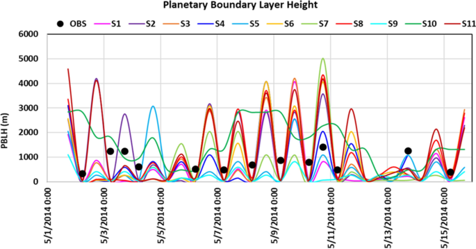
Planetary boundary layer height (model simulations vs observed) where the black circles represent the observations at 0530 and 1730 h
Table 6 Statistical analysis of planetary boundary layer height over Delhi -
e.
Land surface temperature Figs. 6 and 7 show average LST from WRF model simulations (S1 to S11) and TERRA-MODIS (OBS) during daytime (1:30PM) and nighttime (1:30AM), respectively. It can be seen that all the WRF model schemes overestimate LST when compared to the satellite data, both during daytime and nighttime.
Fig. 6 
Average land surface temperature from model simulations (S1 to S11) and MODIS aqua (OBS)—daytime (1:30 PM)
Fig. 7 
Average land surface temperature from model simulations (S1 to S11) and MODIS Aqua (OBS)—nighttime (1:30 AM)
Large differences are seen between LST from different model simulations. During daytime S4, S5, S6, S8 S10 and S11 Schemes show highest LST (between 320 and 330 K) compared to other schemes. It should be noted that these schemes use GBM, Shin-Hong, BouLac and UW PBL and revised MM5 surface layer scheme. S1, S2 and S3 schemes using ACM2 PBL scheme and Pleim surface layer show comparatively lower LST values with maximum LST value of 322 K. S7 and S9 both simulate lower LST values compared to the rest of the schemes. S7 scheme is driven by MYJ PBL and Eta surface layer and S9 using TEMF PBL and surface layer scheme. It is seen that during daytime S7 scheme shows higher LST and S9 scheme shows lowest LST over urban areas compared to other LULC classes (LULC classes shown in Fig. 1b).
During the night, all the schemes (except S1, S2 and S3) show higher LST values over urban areas following the urban signature compared to other LULC classes. Out of all the schemes, S7 simulates highest (304–312 K) LST over Delhi-NCR. Overall, it is seen that S9 (TEMF) well captures daytime and nighttime LST with lower bias compared to other PBL schemes.
-
f.
Solar radiation and surface fluxes Fig. 8 shows the diurnal variation of incoming shortwave radiation (SWDOWN), sensible heat flux (HFX) and latent heat flux (LH) over Delhi. It is observed that during daytime S9 (TEMF PBL) scheme simulates lowest incoming shortwave radiation and heat flux values compared to rest of the simulations. The reduced incoming solar radiation with TEMF PBL scheme (S9) could be attributed to the greater amount of boundary-layer clouds; this inference is depicted in Fig. 9 which gives the average cloud fraction for model simulations S1 to S11. It is noted that S9 simulation (TEMF scheme), shows greater amount of clouds in comparison to other simulation sets. We have seen in above sections that S9 shows lower values (and best estimates) of near-surface and land surface temperature during daytime. Thus, it can be inferred that difference between simulated near surface/land surface temperature is closely related with difference in simulated incoming solar radiation/heat fluxes. S1, S2 and S3 schemes (using Pleim-Xiu LSM) exhibit higher latent heat flux compared to other schemes (using Noah LSM). Sun et al. (2017) also reported higher latent heat flux values with Pleim-Xiu LSM compared to Noah LSM.
Fig. 8 
Diurnal variation of shortwave radiation, sensible heat flux and latent heat flux over Delhi
Fig. 9 
Average cloud fraction from model simulations (S1 to S11)
During nighttime, there are small differences in the sensible and latent heat flux simulated by different schemes, but some differences are seen between the simulated LST with S7 (MYJ + Eta) showing highest surface temperatures. This may be attributed to the accumulation of large heat flux stored in the soil during daytime which gets transported to the surface and causes warmer land surface temperature during nighttime.


It is observed that with the radiation schemes fixed to Dudhia short wave and RRTM long wave (which works best for the study region); irrespective of the PBL and SL combinations, the Noah LSM which has been used in simulation sets S4–S11 performs better than Pleim-Xiu LSM. The simulation set best for T2 (overall S9, nocturnal S7), RH (overall S9), PBLH (S6) and LST (S10) inherently has Noah LSM scheme and is deemed suitable for the study region. A brief description of Noah LSM is given in Appendix 1.
Based on the various statistical evaluation performed for different meteorological parameters it can be inferred that TEMF PBL simulation set works best for the surface temperature, land surface temperature and relative humidity, ACM2 shows good agreement for surface wind speed. GBM PBL scheme gives better agreement for planetary boundary layer height compared to other schemes over the study region. This may be because in GBM vertical fluxes of TKE are enhanced for better comparison to large eddy simulations. In TEMF, vertical mixing is estimated by eddy diffusivity and mass flux. The eddy diffusivity is calculated from total turbulent energy (TE) which is the sum of TKE and turbulent potential energy. ACM2 PBL uses nonlocal upward mixing and local downward mixing. It should be noted that both TEMF and ACM2 PBL schemes are designed as hybrid (local-nonlocal) schemes. Thus, it can be seen that the near-surface meteorological parameters are depicted with greater accuracy when both local and nonlocal viewpoints are considered. It is seen that the wind speed and relative humidity were within the benchmark for the best performing scheme, in terms of MB, MAGE and RMSE; whereas for Temperature errors were found to be on higher side of the acceptable benchmark. The evaluation results indicate that by selecting the scheme showing the best representation of the surface and atmospheric processes for the current application, errors owing to the physical parameterizations in the model can be reduced. To further address the model biases it is important to refine the physical parameterizations schemes in the WRF model or using different bias correction and data assimilation techniques. The model performance evaluation based on analysis of diurnal trends and various statistical parameters for the present study region gives the confidence to employ the model for further application to forecast meteorological variables.
5 Conclusions
The present study assessed the WRF model performance over National Capital Region of India during the summer period in simulating various meteorological variables for various physical parameterizations relating to shortwave and longwave radiation, surface layer, planetary boundary layer and land surface model parameterization schemes. The analysis of diurnal trends and various statistical schemes reveal:
-
The Dudhia shortwave and RRTM longwave radiation combination schemes work best with higher agreement indices and lower errors compared to New Goddard and RRTMG radiation scheme for Temperature and Relative Humidity for the study region.
-
Simulations with all the PBL schemes show overestimation for near surface Temperature during daytime and nighttime except ACM2 PBL and Pleim-Xiu SL combination which differ in nocturnal temperature trend showing underestimation.
-
For Relative Humidity, all the Radiation and PBL schemes show underestimation both during daytime and nighttime.
-
It is seen that with the best performing scheme, simulated Wind Speed and Relative Humidity are found to be within the standard statistical benchmark whereas simulated temperature lies on the higher side of the acceptable range. Model shows overestimation for Land Surface Temperature compared to the satellite data, both during daytime and nighttime with all the parameterization schemes.
-
Overall based on statistical analysis, TEMP PBL scheme (S9) performs best for near surface Temperature, Land Surface Temperature and Relative Humidity over the study region while Boulac scheme performs the second best for near surface temperature and relative humidity.
-
The combination of ACM2 PBL and Pleim-Xiu SL and LSM schemes are best suited to estimate Wind Speed for the region, with New Goddard radiation schemes showing better performance for daytime and RRTMG radiation schemes for nighttime while Shin Hong PBL scheme performs second best for wind speed.
-
GBM PBL scheme performs best estimates for Planetary Boundary Layer Height over Delhi.
-
Noah LSM performs better than the Pleim-Xiu LSM in simulating various meteorological variables.
-
It is inferred that TEMF PBL simulation set works best for the study region and can be employed for further application of the model to forecast meteorological parameters.
References
Angevine WM, Jiang H, Mauritsen T (2010) Performance of an Eddy diffusivity-mass flux scheme for shallow cumulus boundary layers. Mon Weather Rev 138:2895–2912. https://doi.org/10.1175/2010MWR3142.1
Avolio E, Federico S, Miglietta MM et al (2017) Sensitivity analysis of WRF model PBL schemes in simulating boundary-layer variables in southern Italy: an experimental campaign. Atmos Res 192:58–71. https://doi.org/10.1016/j.atmosres.2017.04.003
Banks RF, Tiana-Alsina J, Baldasano JM et al (2016) Sensitivity of boundary-layer variables to PBL schemes in the WRF model based on surface meteorological observations, lidar, and radiosondes during the HygrA-CD campaign. Atmos Res 176–177:185–201. https://doi.org/10.1016/j.atmosres.2016.02.024
Bennett ND, Croke BFW, Guariso G et al (2013) Characterising performance of environmental models. Environ Model Softw 40:1–20. https://doi.org/10.1016/j.envsoft.2012.09.011
Borge R, Alexandrov V, José del Vas J et al (2008) A comprehensive sensitivity analysis of the WRF model for air quality applications over the Iberian Peninsula. Atmos Environ 42:8560–8574. https://doi.org/10.1016/j.atmosenv.2008.08.032
Bougeault P, Lacarrère P (1989) Parameterization of orography induced turbulence in a mesobeta-scale model. Mon Weather Rev 117:1872–1890
Bretherton CS, Park S (2009) A new moist turbulence parameterization in the community atmosphere model. J Clim 22:3422–3448. https://doi.org/10.1175/2008JCLI2556.1
Chen F, Dudhia J (2001) Coupling an Advanced Land Surface-Hydrology Model with the Penn State–NCAR MM5 Modeling System. Part I: model implementation and sensitivity. Mon Weather Rev 129:569–585. https://doi.org/10.1175/1520-0493(2001)129%3c0569:CAALSH%3e2.0.CO;2
Chou M-D, Suarez MJ. A solar radiation parameterization (CLIRAD-SW) for Atmospheric Studies. 48
Di Z, Gong W, Gan Y et al (2019) Combinatorial optimization for WRF physical parameterization schemes: a case study of three-day typhoon simulations over the Northwest Pacific Ocean. Atmosphere 10:233. https://doi.org/10.3390/atmos10050233
Dudhia J (1989) Numerical study of convection observed during the winter monsoon experiment using a mesoscale two-dimensional model. J Atmos Sci 46:3077–3107
El-Kawy OA, Rød JK, Ismail HA, Suliman AS (2011) Land use and land cover change detection in the western Nile delta of Egypt using remote sensing data. Appl Geogr 31:483–494. https://doi.org/10.1016/j.apgeog.2010.10.012
Emery C, Tai E, Yarwood G (2001) Enhanced meteorological modeling and performance evaluation for two Texas ozone episodes. Prepared for the Texas natural resource conservation commission, by ENVIRON International Corporation
Gallo KP, Easterling DR, Peterson TC (1996) The influence of land use/land cover on climatological values of the diurnal temperature range. J Climate 9:2941–2944
Gevorgyan A (2018) A Case Study of Low-Level Jets in Yerevan Simulated by the WRF Model. J Geophys Res 123(1):300–314. https://doi.org/10.1002/2017JD027629
Grenier H, Bretherton CS, Moist PBL (2001) Parameterization for large-scale models and its application to subtropical cloud-topped marine boundary layers. Mon Weather Rev 129:357–377. https://doi.org/10.1175/1520-0493(2001)129%3c0357:AMPPFL%3e2.0.CO;2
Güler M, Yomralıoğlu T, Reis S (2007) Using landsat data to determine land use/land cover changes in Samsun, Turkey. Environ Monit Assess 127:155–167. https://doi.org/10.1007/s10661-006-9270-1
Gunwani P, Mohan M (2017) Sensitivity of WRF model estimates to various PBL parameterizations in different climatic zones over India. Atmos Res 194:43–65. https://doi.org/10.1016/j.atmosres.2017.04.026
Hariprasad KBRR, Srinivas CV, Singh AB et al (2014) Numerical simulation and intercomparison of boundary layer structure with different PBL schemes in WRF using experimental observations at a tropical site. Atmos Res 145–146:27–44. https://doi.org/10.1016/j.atmosres.2014.03.023
Hu X-M, Nielsen-Gammon JW, Zhang F (2010) Evaluation of Three Planetary Boundary Layer Schemes in the WRF Model. J Appl MeteorolClimatol 49:1831–1844. https://doi.org/10.1175/2010JAMC2432.1
Iacono MJ, Delamere JS, Mlawer EJ et al (2008) Radiative forcing by long-lived greenhouse gases: calculations with the AER radiative transfer models. J Geophys Res. https://doi.org/10.1029/2008JD009944
IMD Bulletin, May 2014, http://wamis.org/countries/india/indsum_20140509.pdf
Janjic ZI (1996) The surface layer in the NCEP Eta Model. In: Eleventh conference on numerical weather prediction. http://www2.mmm.ucar.edu/wrf/users/phys_refs/SURFACE_LAYER/eta_part3.pdf
Janjic ZI (2001) Nonsingular Implementation of the Mellor–Yamada Level 2.5 Scheme in the NCEP Meso model, National Centres for Environmental Prediction (NCEP) Office Note. http://citeseerx.ist.psu.edu/viewdoc/download?doi=10.1.1.459.5434&rep=rep1&type=pdf
Janjić ZI (1994) The step-mountain eta coordinate model: further developments of the convection, viscous sublayer, and turbulence closure schemes. Mon Wea Rev 122:927–945
Jankov I, Gallus WA Jr, Segal M, Shaw B, Koch SE (2005) The impact of different WRF model physical parameterizations and their interactions on warm season MCS rainfall. Wea. Forecasting. 20:1048–1060. https://doi.org/10.1175/WAF888.1
Jiménez PA, Dudhia J, González-Rouco JF et al (2012) A revised scheme for the WRF surface layer formulation. Mon Weather Rev 140:898–918. https://doi.org/10.1175/MWR-D-11-00056.1
Kain JS (2004) The Kain-fritsch convective parameterization: an update. J Appl Meteorol 43:170–181. https://doi.org/10.1175/1520-0450(2004)043%3c0170:TKCPAU%3e2.0.CO;2
Lacis AA, Hansen J (1974) A parameterization for the absorption of solar radiation in the earth’s atmosphere. J Atmos Sci 31:118–133. https://doi.org/10.1175/1520-0469(1974)031%3c0118:APFTAO%3e2.0.CO;2
Lin YL, Farley RD, Orville HD (1983) Bulk parameterization of the snow field in a cloud model. J Climate Appl Met 22:1065–1092. http://www.jstor.org/stable/26180993
Lv Z, Zhou Q (2011) Utility of landsat image in the study of land cover and land surface temperature change. Proc Environ Sci 10:1287–1292. https://doi.org/10.1016/j.proenv.2011.09.206
Madala S, Satyanarayana ANV, Rao TN (2014) Performance evaluation of PBL and cumulus parameterization schemes of WRF ARW model in simulating severe thunderstorm events over Gadanki MST radar facility—case study. Atmos Res 139:1–17. https://doi.org/10.1016/j.atmosres.2013.12.017
Mahapatra B, Walia M, Saggurti N (2018) Extreme weather events induced deaths in India 2001–2014: trends and differentials by region, sex and age group. Weather Clim Extremes 21:110–116. https://doi.org/10.1016/j.wace.2018.08.001
Michalakes J, Dudhia J, Gill D, Henderson T, Klemp J, Skamarock W, Wang W (2005) The weather research and forecast model: software architecture and performance. Proc Ele ECMWF Works Use High Perf Comput Meteorol. https://doi.org/10.1142/9789812701831_0012
Mlawer EJ, Taubman SJ, Brown PD et al (1997) Radiative transfer for inhomogeneous atmospheres: RRTM, a validated correlated-k model for the longwave. J Geophys Res Atmos 102:16663–16682. https://doi.org/10.1029/97JD00237
Mohan M, Bhati S (2011) Analysis of WRF model performance over subtropical region of Delhi, India. Adv Meteorol 2011:1–13. https://doi.org/10.1155/2011/621235
Mohan M, Gupta M (2018) Sensitivity of PBL parameterizations on PM10 and ozone simulation using chemical transport model WRF-Chem over a sub-tropical urban airshed in India. Atmos Environ 185:53–63. https://doi.org/10.1016/j.atmosenv.2018.04.054
Mohan M, Sati AP (2016) WRF model performance analysis for a suite of simulation design. Atmos Res 169:280–291. https://doi.org/10.1016/j.atmosres.2015.10.013
National Capital Region Planning Board (Ministry of Housing and Urban Affairs, Government of India). http://ncrpb.nic.in/
Noilhan J, Planton S (1989) A simple parameterization of land surface processes for meteorological models. Mon Weather Rev 117:536–549. https://doi.org/10.1175/1520-0493(1989)117%3c0536:ASPOLS%3e2.0.CO;2
Panda J, Sharan M (2012) Influence of land-surface and turbulent parameterization schemes on regional-scale boundary layer characteristics over northern India. Atmos Res 112:89–111. https://doi.org/10.1016/j.atmosres.2012.04.001
Patil R, Pradeep Kumar P (2016) WRF model sensitivity for simulating intense western disturbances over North West India. Model Earth Syst Environ. https://doi.org/10.1007/s40808-016-0137-3
Pleim JE (2007a) A combined local and nonlocal closure model for the atmospheric boundary layer. Part II: application and evaluation in a mesoscale meteorological model. J Appl MeteorolClimatol 46:1396–1409. https://doi.org/10.1175/JAM2534.1
Pleim JE (2007b) A combined local and nonlocal closure model for the atmospheric boundary layer. Part I: model description and testing. J Appl MeteorolClimatol 46:1383–1395. https://doi.org/10.1175/JAM2539.1
Pleim JE, Gilliam R (2009) An indirect data assimilation scheme for deep soil temperature in the Pleim-Xiu land surface model. J Appl MeteorolClimatol 48:1362–1376. https://doi.org/10.1175/2009JAMC2053.1
Pleim JE, Xiu A (2003) Development of a land surface model. Part II: data assimilation. J Appl Meteorol 42:1811–1822. https://doi.org/10.1175/1520-0450(2003)042%3c1811:DOALSM%3e2.0.CO;2
Sathyanadh A, Prabha TV, Balaji B et al (2017) Evaluation of WRF PBL parameterization schemes against direct observations during a dry event over the Ganges valley. Atmos Res 193:125–141. https://doi.org/10.1016/j.atmosres.2017.02.016
Sati AP, Mohan M (2018) The impact of urbanization during half a century on surface meteorology based on WRF model simulations over National Capital Region, India. Theor Appl Climatol 134:309–323. https://doi.org/10.1007/s00704-017-2275-6
Shin HH, Hong S-Y (2015) Representation of the subgrid-scale turbulent transport in convective boundary layers at Gray-Zone resolutions. Mon Weather Rev 143:250–271. https://doi.org/10.1175/MWR-D-14-00116.1
Shrivastava R, Dash SK, Oza RB, Sharma DN (2014) Evaluation of parameterization schemes in the WRF model for estimation of mixing height. Int J Atmos Sci 2014:1–9. https://doi.org/10.1155/2014/451578
Skamarock WC, Klemp JB, Dudhia J, Gill DO, Barker DM, Duda MG, Huang X-Y, Wang W, Powers JG (2008) A description of the advanced research WRF Version 3. Mesoscale and Microscale Meteorology Division, NCAR, Boulder, pp 1–3
Stephens GL (1978) Radiation profiles in extended water clouds. II: parameterization Schemes. J Atmos Sci 35:2123–2132. https://doi.org/10.1175/1520-0469(1978)035%3c2123:RPIEWC%3e2.0.CO;2
Sun X, Holmes HA, Osibanjo OO, Sun Y, Ivey CE (2017) Evaluation of surface fluxes in the WRF Model: case study for farmland in rolling terrain. Atmosphere 8(10):197. https://doi.org/10.3390/atmos8100197
Tian Y, Miao J (2019) A numerical study of mountain-plain breeze circulation in Eastern Chengdu, China. Sustainability 11:2821. https://doi.org/10.3390/su11102821
Tyagi B, Magliulo V, Finardi S et al (2018) Performance analysis of planetary boundary layer parameterization schemes in WRF modeling set up over Southern Italy. Atmosphere 9:272. https://doi.org/10.3390/atmos9070272
Willmott CJ, Robeson SM, Matsuura K (2012) A refined index of model performance. Int J Climatol 32:2088–2094. https://doi.org/10.1002/joc.2419
Xie B, Fung JCH, Chan A, Lau A (2012) Evaluation of nonlocal and local planetary boundary layer schemes in the WRF model: evaluation of PBL schemes in WRF. J Geophys Res Atmos 117:1. https://doi.org/10.1029/2011JD017080
Zeyaeyan S, Fattahi E, Ranjbar A et al (2017) Evaluating the effect of physics schemes in wrf simulations of summer rainfall in North West Iran. Climate 5:48. https://doi.org/10.3390/cli5030048
Acknowledgements
This study is a part of the project entitled “Incorporation of realistic landuse–landcover features in regional numerical models for improving predictions of temperature and rainfall over National Capital Region of India” funded by the Department of Science and Technology, Government of India [Sanction number: DST/CCP/NCM/68/2017 (G) dated 02.03.2017]. The authors thank IIT Delhi HPC facility for computational resources. We acknowledge the use of data products from Level-1 and Atmosphere Archive & Distribution System (LAADS) Distributed Active Archive Center (DAAC), located in the Goddard Space Flight Center in Greenbelt, Maryland.
Author information
Authors and Affiliations
Corresponding author
Additional information
Responsible Editor: Junfeng Miao.
Publisher's Note
Springer Nature remains neutral with regard to jurisdictional claims in published maps and institutional affiliations.
Appendices
Appendices
1.1 Appendix 1
See Table 7.
1.2 Appendix 2
Statistical measures used for Model Evaluation based on previous studies (Willmott et al. 2012; Sati and Mohan 2016; Gunwani and Mohan, 2017; Emery et al. 2001).
Following statistical parameters have been used in the present study.
-
Index of agreement (IOA)
$$ IOA = 1 - \frac{{\mathop \sum \nolimits_{i = 1}^{n} \left| {Pi - Oi} \right|}}{{2\mathop \sum \nolimits_{i = 1}^{n} \left| {Oi - \bar{O}} \right|}} $$when \( \mathop \sum \nolimits_{i = 1}^{n} \left| {Pi - Oi} \right| \le 2\mathop \sum \nolimits_{i = 1}^{n} \left| {Oi - \bar{O}} \right| \) and
$$ IOA = \frac{{2\mathop \sum \nolimits_{i = 1}^{n} \left| {Oi - \bar{O}} \right|}}{{\mathop \sum \nolimits_{i = 1}^{n} \left| {Pi - Oi} \right|}} - 1 $$when \( \mathop \sum \nolimits_{i = 1}^{n} \left| {Pi - Oi} \right| > 2\mathop \sum \nolimits_{i = 1}^{n} \left| {Oi - \bar{O}} \right| \) IOA ranges between -1 and 1 (Willmott et al. 2012).
-
Mean bias (MB)
$$ {\text{MB}} = {\bar{\text{P}}} - {\bar{\text{O}}} $$ -
Mean absolute gross error (MAGE)
$$ MAGE = \frac{1}{N}\mathop \sum \limits_{i = 1}^{N} \left| {Pi - Oi} \right| $$ -
Root mean square error (RMSE)
$$ {\text{RMSE}} = \sqrt {\frac{{\mathop \sum \nolimits_{{{\text{i}} = 1}}^{\text{N}} \left( {{\text{Pi}} - {\text{Oi}}} \right)^{2} }}{\text{N}}} $$where Pi, Oi, \( \underset{\raise0.3em\hbox{$\smash{\scriptscriptstyle-}$}}{P} \) and \( \underset{\raise0.3em\hbox{$\smash{\scriptscriptstyle-}$}}{O} \) represent predicted data, observed data, predicted mean and observed mean respectively. Statistical benchmarks for the meteorological parameters (Emery et al. 2001; Sati and Mohan 2016; Gunwani and Mohan 2017)—Temperature Mean Bias ± 0.5 K, MAGE 2 K, RMSE 2 K; Wind Speed Mean Bias ± 0.5 m/s, MAGE 2 m/s, RMSE 2.0 m/s; Relative Humidity Mean Bias < 10%, RMSE < 20%.
Rights and permissions
About this article

Cite this article
Gunwani, P., Sati, A.P., Mohan, M. et al. Assessment of physical parameterization schemes in WRF over national capital region of India. Meteorol Atmos Phys 133, 399–418 (2021). https://doi.org/10.1007/s00703-020-00757-y
Received:
Accepted:
Published:
Issue Date:
DOI: https://doi.org/10.1007/s00703-020-00757-y