
Abstract
This paper presents the mechanism and control design of a micro-motion stage, which employs the right-angle flexure hinges and piezoelectric actuators (PZT). Aiming at the mechanism with the characteristics of a large stroke and three degrees of freedom, analytical models of statics and dynamics are established; especially the coupling motions of stage are investigated, which are verified by finite element analysis simulation. Via open-loop experiment, the decoupling property is well certified. Owing to the hysteresis of PZT, the dynamic equation of system with Bouc–Wen hysteresis model is proposed, which is identified through the Least squares. Moreover, a closed-loop controller of proportion integral derivative combined with the inverse hysteresis model-based feedforward is developed to reduce the nonlinearity and uncertainty, which can improve the positioning accuracy. Besides, the single-axis and multi-axis motions are tested. Experimental results reveal that the stage has a well-decoupling performance, and the effectiveness of proposed Bouc–Wen model is validated under open-loop control. Furthermore, the micro-motion performance in single- and multi-axis motions can be achieved as well.
1 Introduction
Recently, micro- and nano-manipulators have become the hot research topic, because they play an increasingly important role in micro and nanotechnologies, such as the Nano Mask Aligner, the biomedical operation, the micro electro mechanical system (MEMS), the atomic force microscope (AFM), and the ultrahigh precision machining, etc. (Liu et al. 2015; Choi and Han 2007). Instead of traditional manipulator, numerous compliant mechanisms appear continuously that are developed to deliver the micro- and nano-scale motion by making use of elastic deformations of material. And the compliant mechanisms provide the merits including no friction, no backlash, high motion sensitivity and great motion repeatability (Jiang et al. 2015; Lin et al. 2018b). As a result, the studies of compliant micro-motion platform which can achieve the micro- and nano-motion have been widely concerned all over the world (Xu 2013; Tian et al. 2011; Ling et al. 2017).
In recent advances, many compliant stages were proposed, which are generally classified into serial and parallel structures. However, serial stages have the expensive of limited freedom, high inertia and cumulative errors, possessing the advantages of large stroke, simple structure and control strategy simultaneously (Kim et al. 2012; Shan et al. 2012). Parallel stages contribute to low inertia and compact size, while the coupling motion is a hard focus (Li et al. 2012; Zhang et al. 2017). Hence, in order to propose a stage with multiple degrees of freedom and a large stroke, the combination of serial and parallel mechanisms is a very meaningful point. Moreover, decoupling analysis is very beneficial to implement the single–input–single–output (SISO) control for multiple-freedom stages. At present, since the piezoelectric actuators (PZTs) are capable of linear positioning with nanometer level resolution, high stiffness, good stability and large blocking force, they are employed for actuation by many compliant mechanisms or micro- and nano- positioning stages (Dong et al. 2016; Zubir et al. 2009). However, the PZTs include the nonlinearity due to the hysteresis property occurring at voltage-driven method, which will reduce the positioning accuracy of micro-motion stage if not driven error compensation. The common way to treat the shortcoming is the hysteresis model-based control scheme (Wei et al. 2014). This method implements a feedforward compensator based on the inverse hysteresis model that precisely describes the complex hysteretic behavior, then makes use of a closed-loop feedback controller to further suppress the other errors. In the past, a number of hysteresis models are developed, such as the Preisach model (Song et al. 2005; Weibel et al. 2008), the Bouc–Wen model (Lin and Yang 2006), the Maxwell model (Yeh et al. 2008) and the Prandtl-Ishlinskii model (Kuhnen 2003). Compared with other hysteresis models, Bouc–Wen model that describes the mechanical nonlinear system has a practical physical significance, which is more consistent with the mechanical and physical characteristics of PZT. Furthermore, Bouc–Wen model has a fewer parameters and an easier integration with the rest of system model. And as the most difficulty of the model, the identification of parameters has been solved (Wang and Zhu 2011; Razman et al. 2014). According to the inverse hysteresis model, the hysteresis errors of PZT driven by voltage can be successfully compensated. Moreover, the closed-loop controller is combined with the inverse hysteresis to overcome the other nonlinear behaviors, such as the proportional integral derivative (PID) feedback control (Shan and Leang 2012) and the sliding mode control (SMC) (Clark et al. 2015). As the basis of most closed-loop control strategies, PID control is appropriate for preliminary research, which is enough to improve the accuracy of micro-motion. And smarter control strategies will be studied solely as the main content in the next paper.
The major contribution of this paper is to present a compliant mechanism capable of delivering X/Y/Z-axis micromotion with micro scale resolution. The mechanism achieves a large stroke by means of the convex and concave bridge-type amplifiers in series, and possesses a multi-freedom decoupling motion due to the symmetric and parallel distribution of mechanism in X/Y/Z axis. The working principle of input–output has been described (Lin et al. 2016). However, it is far from enough. In this work, analytical models for the fundamental characteristics of mechanism in terms of statics, dynamics and decoupling are conducted, and the decoupling performance is validated by Finite Element Analysis (FEA) simulation and the open-loop experiment. Moreover, taken into account, the hysteresis of PZT is tested by the experiment and modeled by the Bouc–Wen model. Considering this analysis, a control strategy employing the inverse Bouc–Wen model-based feedforward plus a proportional integral derivative (PID) feedback control is implemented in the XYZ stage to reduce the nonlinear effects and achieve the accuracy positioning. Finally, the conclusions are given and future works are discussed.
2 Stage modeling and analysis
Combining the Compliant Mechanisms, Machine design and Innovative Design for Mechanism, the CAD model of designed XYZ stage is shown in Fig. 1. The Fig. 1b, c are respectively the top view and left view of component, which is shown in Fig. 1a.

CAD model of the XYZ micromotion stage
The right-angle flexure hinges are employed to transmit the motion and energy in the stage actuated by PZT, and the input displacement of PZT is amplified by bridge-type amplifier (Kim et al. 2003). Thus, the ultra-precision positioning and large workspace can be achieved. And in accordance with the decoupling requirement, the completely symmetric distribution is designed.
2.1 Statics modeling
The static analyses of stage are conducted by making use of the pseudo-rigid-body (PRB) method (Howell 2013). Owing to the symmetry of bridge-type amplifier, only the quarter is considered. In actual work, the flexure hinge is equivalent to the revolute joint with 1-DOF (Degree of Freedom), and other components are all considered as rigid bodies. The PRB model is denoted in Fig. 2. In the equilibrium status, the equation of 1/4 bridge-type amplifier and the moment are derived as follows:
where \( K_{r} \) and \( \Delta \alpha \) are respectively the rotational stiffness and deformation of right-angle hinge. \( \alpha \) is the slant-angle of arm in amplifier, and \( l_{y} = l_{a} \cdot \sin \alpha \). Hence, the equation is derived as
where \( \Delta y \) denotes the output displacement of 1/4 displacement amplifier. And the major potential energy of bridge-type of amplifier is contributed by the rotational energy of eight hinges. Therefore, the equation is generated as
Thus, the output stiffness of amplifier is expressed as

PRB model of 1/4 bridge-type amplifier
And the \( F_{y} \) is obtained as follows:
Combining the equations of (1)–(6), the \( \Delta \alpha \) is written as
Based on the Principle of Virtual Work, the equation of 1/4 displacement amplifier is deduced as
where \( \Delta x \) is the input of amplifier. Therefore, the \( \Delta x \) is given as
In addition, the input rod of amplifier is also considered. As shown in Fig. 2, the angular deflection of input rod under the moment M is derived by the Bernoulli–Euler method.
where x, y denote the coordinate axis along the neutral axis. \( M\left( y \right) \) is the moment at position y along the neutral axis; \( I\left( y \right) \) is the area moment of inertia. E is the Young’s modulus of the material. The static equilibrium equation at position O is derived as
Thus, the equation at position y is written as
Combining the formulas of (2), (7) and (11), the \( M\left( y \right) \) is written as
Based on the equations of (10), (13), and the boundary conditions are considered, the angular deflection of input rod in X direction is denoted as
Therefore, the angular deflection \( \Delta x_{2} \) at position \( A_{0} \) along x direction is calculated as
Thus, the overall input displacement \( \Delta x_{in} \) actuated by \( F_{x} \) is expressed as follows:
The input stiffness and amplification ration of bridge-type amplifier are given as
2.2 Kinematics modeling
First of all, based on the Lagrange’s equations, the free-vibration equation of bridge type amplifier is written as
where P and Q are the overall kinetic energy and potential energy of amplifier, and they are calculated as follows:
where J is moment of inertia of arm, and \( m_{1} \), \( m_{3} \) are shown in Fig. 2, q is the variable. Therefore, the equivalent mass \( M_{b} \) and stiffness \( K_{b} \) of amplifier can be obtained. In order to analyze the kinematic performance of stage, the Lagrange’s equation is employed.
where U and V are respectively the overall kinetic energy and potential energy of stage. Because of the symmetrical structure, the same results are obtained in X or Y direction. Hence, take the X-motion for example. When the main displacement \( t_{x} \) in X direction is produced, the major elastic deformations are considered, such as the bridge-type amplifier in X direction and four hinges in Y direction, which are distributed at the bottom of both sides. When the main displacement \( t_{z} \) is produced in Z direction, the deformations of eight bridge-type amplifier are mainly considered. Thus, the energy equations of stage can be calculated as follows:
where \( M_{s} \) and \( M_{p} \) are respectively the mass of working-table and parallel-guiding mechanism in Z axis. \( L_{1} \) denotes the arm length of branch chain in vertical direction, which is given in Fig. 3. Thus, considering equations of (20) and (21), the dynamic model of the stage under external load is written as
where \( {\mathbf{M}} = \left[ {M_{x} ,M_{y} ,M_{z} } \right]^{T} \),\( {\mathbf{K}} = \left[ {K_{x} ,K_{y} ,K_{z} } \right]^{T} \) and \( {\mathbf{F}} = \left[ {\hat{F}_{x} ,\hat{F}_{y} ,\hat{F}_{z} } \right]^{T} \) respectively represent the equivalent mass, equivalent stiffness and external load of the stage in X/Y/Z-axis. \( {\mathbf{C}} = \left[ {C,C,C} \right]^{T} \) and \( {\mathbf{q}} = \left[ {q,q,q} \right]^{T} \) respectively denote the damping factor of material and the variable of stage in X/Y/Z-axis.

Model of coupling motion
2.3 Coupling motion modeling
In order to satisfy the requirements of ultra-precision positioning, the research of coupling motion is essential. The coupling motion models of stage in plane X–Y, X–Z are shown in Fig. 3.
For example, when the main displacement \( \delta_{x} \) is produced in X direction, and the coupling displacements \( \Delta y \), \( \Delta z \) are also existing, which are named coupling errors in cross-axis. Therefore, the equations of coupling errors are expressed as
where \( L_{1} ,{\kern 1pt} {\kern 1pt} {\kern 1pt} {\kern 1pt} {\kern 1pt} L_{2} \) are respectively the arm lengths of branch chains in Y, Z directions. And the approximate formulas of \( \beta \) and \( \gamma \) are shown as follows:
Thus, the coupling errors \( \Delta y \), \( \Delta z \) are derived by combining equations of (23) and (24)
Similarly, when the main displacement \( \delta_{z} \) is produced in Z direction, the coupling errors can be calculated in cross-axis directions. In order to evaluate the coupling performance of stage, the coupling ratio is employed, which is expressed as \( \eta = {\Delta \mathord{\left/ {\vphantom {\Delta \delta }} \right. \kern-0pt} \delta } \times 100\% . \) Thus, the decoupling capability of stage can be obtained.
3 Model validation with FEA
The simulation study is carried out with FEA software (ANSYS). The deformations of X/Y/Z axis with different input are given in Figs. 4, 5. An external force is assigned at the position of output, the output stiffness and coupling errors with simulation are obtained. For comparison, the performances are tabulated in Table 1. It is observed that the predicted results of output stiffness (\( K_{out}^{stage} \)) in X/Y or Z direction are respectively 18.3 N/mm and 25.6 N/mm.

Output of X/Y axis with input of 20 μm

Output of Z axis with input of 10 μm
However, the FEA results are 19.0 N/mm and 24.1 N/mm. And the relative errors are 3.7% and 6.2%, respectively. Meanwhile, the input stiffness of stage (\( K_{in}^{stage} \)) is described, and the relative errors are less than 10%. It is noticeable that the input stiffness is less than the minimum stiffness of PZT (Pst-40VS15: 60 N/μm), which means the PZT can be adopted to actuate the stage. Besides, the range of coupling ratio is 0.03 ~ 0.09%, which indicates a well-decoupling property of XYZ stage. Thus, it is noticeable that the reasonability of model is verified.
4 Control strategy and experiments
In this section, the prototype of the XYZ stage is fabricated and the experiments are conducted to report the performance of the XYZ stage.
4.1 Experimental setup
The developed prototype of XYZ positioning sage is shown in Fig. 6. The micro-stage is machined by the wire electric discharge machining (WEDM) utilizing the material of AZ31b alloy. The low-voltage PZT actuators (Pst-40VS15) are employed to drive the bridge amplification mechanism. And each PZT is actuated by the linear voltage controller (model: E01.D3). The output displacement of stage is measured by the capacitive displacement sensors (model: CS5), which is supported by magnetic base. And the measuring range of sensor is 0 to 5 mm. Besides, the displacement resolution of sensor is 0.015% FSO, and the linearity is 0.3% FSO. Furthermore, the measured data are delivered to the computer to achieve the display.

Experimental setup of the positioning stage
4.2 Open-loop experiment
The micro-motion accuracy of stage is seriously influenced by the hysteresis of PZT under open-loop control. Hence, the experimental tests with open-loop are conducted to analyze the performance of stage. For instance, a 0.5-Hz input voltage signal is applied to the PZTs in X/Y and Z-axis, and the range of voltage is 0–120 V, the results are shown in Fig. 7.

Output motion of X/Y, Z-axis with PZTs driven by sinusoidal voltage input
The hysteresis of output displacement is observed obviously, and there is a large hysteresis error between voltage-up and voltage-down, which has a large influence on the positioning performance of stage. Besides, the nice output linearity is presented in the range of 40–100 V. And the linearity of voltage-up process is better than the voltage-down process. The output displacements of stage in X/Y- and Z-axis are respectively 238 μm and 202 μm, therefore, T the linearity of stage with ideal condition in X/Y- and Z-axis are respectively 1.98 μm/V and 1.68 μm/V. Thus, there is a big input error caused by hysteresis. In order to improve the positioning precision, the input error of hysteresis must be modeled and compensated.
The Bouc–Wen hysteresis model is employed to simulate the hysteresis of PZT, the dynamic model of the entire micro-motion system with hysteresis can be established as follows:
where the parameters m, c, k, and x are respectively the mass, damping coefficient, stiffness and output displacement in X/Y/Z-axis. \( k_{v} \) denotes the piezoelectric coefficient, \( v\left( t \right) \) is the input voltage, and \( \Delta s \) represents the hysteresis error of PZT. Based on the Bouc–Wen model, the relation between input voltage and output displacement is expressed as
According to the Bouc–Wen model, the hysteresis displacement is written as
where a, b, c are coefficients, n denotes the order of hysteresis, and n = 1 in this work. According to the values of hysteresis displacement (\( \Delta s \)) and differential of voltage (\( \dot{v}\left( t \right) \)), the model is divided as follows
In particular, the Least squares method is adopted in the current problem due to its superiority of optimization performance over other ways. Then the Bouc–Wen hysteresis model of positioning stage can be established by Eq. (26). With a 120 V/0.5 Hz sinusoidal input voltage applied to the PZT, the compensated Bouc–Wen hysteresis models of stage by Eq. (26) are described in Fig. 8. The hysteresis errors are compensated greatly, which certifies the validity of the hysteresis model.

Compensated Bouc–Wen hysteresis model of stage in X/Y- or Z-axis
Besides, in order to describe the decoupling performance, the decoupling test is conducted. The primary output displacement and coupling displacement of stage is recorded and collected. The experimental results are shown in Figs. 9, 10, 11. Because of the symmetry of X–Y, the coupling results in X- or Y-axis are similar. There are coupling results of X–Y, X–Z, Z–X. With a 40 μm/0.5 Hz sinusoidal input signal, the output results are measured. In Fig. 9, the output displacement in X-axis is 262.64 μm, and the coupling displacement in Y-axis is 4.628 μm. The coupling ratio of X–Y is 1.76%. In Fig. 10, the coupling displacement in Z-axis is 3.091 μm. The coupling ratio of X–Z is 1.18%. In Fig. 11, the output displacement in Z-axis is 222.96 μm, and the coupling displacement in X-axis is 2.146. The coupling ratio of Z–X is 0.96%. As a result, the coupling error of positioning stage is less than 2%, which indicates the coupling motion is negligible in comparison to the primary motion. Thus a well-decoupling performance can be achieved. In addition, from the Figs. 9, 10, 11, the coupling curve in X–Y is a clear and normative sinusoidal wave. However, the coupling curve of X–Z and Z–X is an aberrant and nonstandard sinusoidal wave. That is because the complexity of coupling motion and the nonsymmetrical structure in plane of X–Z.

X-axis output displacement and coupling displacement in Y axis

X-axis output displacement and coupling displacement in Z axis

Z-axis output displacement and coupling displacement in X axis
In a word, the effectiveness of constructed Bouc–Wen model is verified. Therefore, the hysteresis errors of PZT can be compensated by the inverse Bouc–Wen. And a well-decoupling performance is obtained. Furthermore, in order to remove the driven errors of creep, and other uncertainties, the PID feedback controller is designed later.
4.3 Closed-loop design and experiment
4.3.1 Controller design
The purpose of motion controller design is to achieve a precision positioning once the desired trajectory of X/Y/Z stage is given. Considering the model errors proposed in the previous works, the nonlinear effects cannot be completely compensated by the inverse Bouc–Wen model. Thus, an additional closed-loop controller is employed. Specifically, the PID controller is adopted due to its robustness. The control scheme is shown in Fig. 12.

Block diagram of designed PID controller
Both the force and displacement generated by PZT are the input source of the stage. However, the output force \( F_{pzt} \) of PZT is reduced under load while the output displacement \( x_{pzt} \) of PZT is amplified by the bridge-type amplifier. Hence, in combination with the dynamic model of the stage in the equations of (22) and (26), the dynamic equation of stage in a single direction of motion is established as
where the parameters y and F are respectively the output displacement and external load of stage in X/Y/Z-axis. Besides, \( \lambda_{amp} \) and \( k_{in} \) respectively represent the actual displacement amplification ratio and the input stiffness of the bridge-type amplifier.
By applying Laplace transform to the equation of (30), the transfer functions in X/Y/Z-axis for the stage between the output displacement and the input displacement can be obtained as
The PID control input in time-domain can be expressed as follows:
where \( e\left( t \right) \) denotes the tracking error, and the three parameters of PID controller \( K_{p} \), \( T_{i} \) and \( T_{d} \) are the proportional gain, integral time and derivative time, respectively. Considering the properties of anti-interference and easy-to-implement, the incremental PID algorithm is adopted. The discretized form of PID controller is derived as
where k denotes the index of time series, T represents the sampling time interval (T = 0.001 s).
In order to identify the control parameters \( K_{p} \), \( T_{i} \) and \( T_{d} \), the Ziegler–Nichols tuning method is employed. Finally, the parameters are identified as follows:
4.3.2 Closed-loop experimental test
-
1.
Comparison under different controller: To demonstrate the applicability of different control method, the simulation studies are performed to obtain the step responses of stage in X axis, as shown in Fig. 13. For a clear comparison, a large oscillation curve can be observed, the \( M_{p} \) of overshoot is 30 μm, and a longer setting time than the standard PID controller is reflected, which is approximately 0.4 s. Even worse, due to other non-linear errors under open-loop control, the statics value is less than the desired value, which largely lowers the positioning precision. In contrast, under the PID control, the setting time is largely shorten, which is more than 50%. And the statics value is approximately equal to the desired value. Thus, the desired trajectory can be achieved. In a word, the simulation results illustrate the effectiveness of the designed PID controller.
Fig. 13 
Results contrast of step responses with different controls
-
2.
Single-Axis Tracking: First, the single-axis tracking experiment is conducted. The output displacement of the stage in theory has been derived and obtained in the previous work (Lin et al. 2018a). With a 10 μm/0.5 Hz square-wave signal applied to PZTs, the X/Y or Z-axis motion response curves are plotted in Figs. 14 and 15. A clear comparison with the oscillation amplitude, the X/Y-motion has the larger step oscillation than the Z-motion, which is because the system is second-order dynamic system, and the stiffness of Z-axis is more excellent to the stiffness of X/Y-axis. And the relative errors between theoretical and experimental in X/Y-axis and Z-axis are respectively 3.01% and 9.38%. Thus, there is a better dynamic property in Z-axis than in X/Y-axis.
Fig. 14 
Results for a 10 μm square-wave in X/Y-axis
Fig. 15 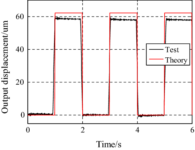
Results for a 10 μm square-wave in Z-axis


Moreover, the motion tracking performances with a 40 μm/0.5 Hz sinusoidal input signal in X/Y/Z axis are also executed. The comparisons between theoretical model output and experimental results of X/Y/Z axis are shown in Figs. 16 and 17. It is observed that the maximum tracking error is 7.56 μm in X/Y axis and the maximum tracking error in Z axis is 23.52 μm. The maximum relative errors between the identified theoretical models and experimental results in X/Y and Z axes are respectively 2.81% and 9.49%. The relative error in Z-axis is larger than in X/Y-axis, which is because the mass of stage and PZTs have a great influence on the motion of Z-axis.

Results for a 40 μm sinusoidal wave in X/Y-axis

Results for a 40 μm/0.5 Hz sinusoidal wave in Z-axis
-
3.
Multi-Axis Tracking: Second, in order to discuss the multi-axis cooperative tracking performance of XYZ stage, the biaxial and triaxial tracking tests are conducted. First of all, by driving the two axes simultaneously in X–Y area with the maximum input of 40 μm, the response results of stage are shown in Fig. 18. The ideal reference tracking is a linear contour along a 45° line with the constant tracking velocity of 10 μm/s, as shown by red line. And the actual tracking is obtained. The stage moves from the home position (0, 0) to (262, 262) and then returns to the home. The maximum tracking error is less than 2 μm, and the maximum relative error is 1.01%. Therefore, the fine linearity is achieved, which indicates that the stage has a nice biaxial motion performance. Similarly, the tracking with an input of three axes driven simultaneously in X–Y–Z area is shown in Fig. 19. The stage moves from home position (0, 0, 0) to (200, 200, 200) and then returns to the home. The ideal reference track is a linear contour along a 45° line. However, because of the influence of coupling motion, the actual track is not well-pleasing. The maximum tracking error is 6.23 μm, and the maximum relative error between the ideal reference tracking and experimental result is 10.25%. Thus, the mediocre triaxial motion performance is demonstrated.
Fig. 18 
Biaxial linear tracking results in X–Y area
Fig. 19 
Triaxial linear tracking results in X–Y–Z area


5 Discussions
The obtained experimental results indicate that the stage has satisfactory performances, such as the well-decoupling motion in cross-axis, the nice biaxial-axis and mediocre triaxial motion properties. Moreover, the limitation of the workspace of stage mainly arises from the maximum output displacement of PZT. Using large-range PZTs, larger workspace can be achieved with the proposed stage. However, the tracking error between the identified theoretical model and experimental results is not perfect, the relative tracking errors in X/Y and Z axis are respectively approximately 3% and 10%, which is effected by many factors, such as the mass of PZT and stage in Z-axis, the machining error, installation error, measurement error, the limit of experimental conditions and other uncertainties. If the high-precision machining and measurement methods are adopted, the more satisfactory results can be obtained. In addition, even though the nonlinear effects of PZT can be weakened by PID control, the fixed control parameters cannot be adapted to the change of reference input. Thus, a more intelligent and sophisticated control schemes will be discussed in future.
6 Conclusions
A completely decoupling micromotion stage with symmetric mechanism actuated by PZTs is proposed. The static analysis is performed by the pseudo-rigid-body (PRB) method, and the dynamic model is established with Lagrange’s equation, especially the coupling motions are investigated. The FEA simulations not only verify the accuracy of derived models but also reveal the nice decoupling performance of XYZ stage. Experimental results under open-loop control demonstrate the bad hysteresis of stage and the Bouc–Wen model is capable of describing the piezoelectric hysteresis accurately. Besides, the desired decoupling motion in cross-axis of stage is obtained, and the coupling ratio between two axes is less than 2%. A closed-loop controller with a PID feedback is constructed, which decreases largely the effect of nonlinearity and compensates the driving errors. A fine output linearity of stage is obtained. With the closed-loop controller of PID, a good performance of stage in single-axis and multi-axis motion is given. Furthermore, the proposed method can be easily extended to other types of micro-motion stage with PZT as well.
References
Choi KB, Han CS (2007) Optimal design of a compliant mechanism with circular notch flexure hinges. Proc Inst Mech Eng Part C J Mech Eng Sci 221:385–392
Clark L, Shirinzadeh B, Bhagat U, Smith J, Zhong Y (2015) Development and control of a two DOF linear–angular precision positioning stage. Mechatronics 32:34–43
Dong R, Tan Y, Xie Y, Janschek K (2016) Recursive identification of micropositioning stage based on sandwich model with hysteresis. IEEE Trans Control Syst Technol 25:317–325
Howell LL (2013) Compliant mechanisms. 21st Century Kinematics. Springer, London, pp 457–463
Jiang Y, Li TM, Wang LP (2015) Stiffness modeling of compliant parallel mechanisms and applications in the performance analysis of a decoupled parallel compliant stage. Rev Sci Instrum 86:095109
Kim JH, Kim SH, Kwak YK (2003) Development of a piezoelectric actuator using a three-dimensional bridge-type hinge mechanism. Rev Sci Instrum 74:2918–2924
Kim YS, Yoo JM, Yang SH, Choi YM, Dagalakis NG, Gupta SK (2012) Design, fabrication and testing of a serial kinematic mems xy stage for multifinger manipulation. J Micromech Microeng 22(22):85029–85038
Kuhnen K (2003) Modeling, identification and compensation of complex hysteretic nonlinearities: a modified Prandtl-Ishlinskii approach. Eur J Control 9:407–418
Li Y, Huang J, Tang H (2012) A compliant parallel XY micromotion stage with complete kinematic decoupling. IEEE Trans Autom Sci Eng 9:538–553
Lin CJ, Yang SR (2006) Precise positioning of piezo-actuated stages using hysteresis-observer based control. Mechatronics 16:417–426
Lin C, Wu Z, Ren Y, Yu H (2016) Characteristic analysis of unidirectional multi-driven and large stroke micro/nano-transmission platform. Microsyst Technol 23:3389–3400
Lin C, Shen Z, Wu Z, Yu J (2018a) Kinematic characteristic analysis of a micro-/nano positioning stage based on bridge-type amplifier. Sens Actuators, A 271:230–242
Lin C, Shen Z, Yu J, Li P, Huo D (2018b) Modelling and analysis of characteristics of a piezoelectric-actuated micro-/nano compliant platform using bond graph approach. Micromachines 9(10):498
Ling M, Cao J, Jiang Z, Lin J (2017) Modular kinematics and statics modeling for precision positioning stage. Mech Mach Theory 107:274–282
Liu P, Yan P, Zhang Z (2015) Design and analysis of an X–Y parallel nanopositioner supporting large-stroke servomechanism. Proc Inst Mech Eng Part C J Mech Eng Sci 229:364–376
Razman MA, Priyandoko G, Yusoff AR (2014) Bouc-wen model parameter identification for a mr fluid damper using particle swarm optimization. Adv Mater Res 903:279–284
Shan Y, Leang KK (2012) Dual-stage repetitive control with Prandtl-Ishlinskii hysteresis inversion for piezo-based nanopositioning. Mechatronics 22:271–281
Shan MC, Wang WM, Ma SY, Liu S, Xie H (2012) Analysis and design of large stroke series flexure mechanism. Nanotechnol Precis Eng 10(3):268–272
Song G, Zhao J, Zhou X, Abreu-Garcia JAD (2005) Tracking control of a piezoceramic actuator with hysteresis compensation using inverse Preisach model. IEEE/ASME Trans Mechatron 10:198–209
Tian Y, Shirinzadeh B, Zhang D, Zhong Y (2011) Modelling and analysis of a three-revolute parallel micro-positioning mechanism. Proc Inst Mech Eng Part C J Mech Eng Sci 225:1273–1286
Wang DH, Zhu W (2011) A phenomenological model for pre-stressed piezoelectric ceramic stack actuators. Smart Mater Struct 20(3):035018
Wei Q, Zhang C, Zhang D, Zhang CJ (2014) Sliding-mode control for piezoelectric actuators based on hysteresis observer. Key Eng Mater 609–610:1271–1276
Weibel F, Michellod Y, Mullhaupt P, Gillet D (2008) Real-time compensation of hysteresis in a piezoelectric-stack actuator tracking a stochastic reference. In: American control conference, pp 2939–2944, 11 Jun 2008
Xu Q (2013) Design and development of a compact flexure-based XY precision positioning system with centimeter range. IEEE Trans Industr Electron 61:893–903
Yeh TJ, Ruo-Feng H, Shin-Wen L (2008) An integrated physical model that characterizes creep and hysteresis in piezoelectric actuators. Simul Model Pract Theory 16(1):93–110
Zhang X, Zhang Y, Xu Q (2017) Design and control of a novel piezo-driven XY parallel nanopositioning stage. Microsyst Technol 23:1067–1080
Zubir MNM, Shirinzadeh B, Tian Y (2009) Development of novel hybrid flexure-based microgrippers for precision micro-object manipulation. Rev Sci Instrum 80:065106
Acknowledgements
This work is supported by the National Natural Science Foundation of China (No. 51675060) and the Fundamental Research Funds for the Central Universities (No. 106112017CDJPT280002).
Author information
Authors and Affiliations
Corresponding author
Additional information
Publisher's Note
Springer Nature remains neutral with regard to jurisdictional claims in published maps and institutional affiliations.
Rights and permissions
About this article

Cite this article
Lin, C., Yu, J., Wu, Z. et al. Decoupling and control of micromotion stage based on hysteresis of piezoelectric actuation. Microsyst Technol 25, 3299–3309 (2019). https://doi.org/10.1007/s00542-019-04501-4
Received:
Accepted:
Published:
Issue Date:
DOI: https://doi.org/10.1007/s00542-019-04501-4