Rethinking k-means clustering in the age of massive datasets: a constant-time approach

Abstract

We introduce a highly efficient k-means clustering approach. We show that the classical central limit theorem addresses a special case (k = 1) of the k-means problem and then extend it to the general case. Instead of using the full dataset, our algorithm named k-means-lite applies the standard k-means to the combination C (size nk) of all sample centroids obtained from n independent small samples. Unlike ordinary uniform sampling, the approach asymptotically preserves the performance of the original algorithm. In our experiments with a wide range of synthetic and real-world datasets, k-means-lite matches the performance of k-means when C is constructed using 30 samples of size 40 + 2k. Although the 30-sample choice proves to be a generally reliable rule, when the proposed approach is used to scale k-means++ (we call this scaled version k-means-lite++), k-means++’ performance is matched in several cases, using only five samples. These two new algorithms are presented to demonstrate the proposed approach, but the approach can be applied to create a constant-time version of any other k-means clustering algorithm, since it does not modify the internal workings of the base algorithm.

1 Introduction

The emerging Fourth Industrial Revolution [1, 2] is characterized by applications that rely on large datasets and intelligent analysis [3]. This new ‘data era’ calls for analysis methods that can handle massive datasets efficiently and accurately. This paper presents such an algorithm for a widely studied data analysis problem, namely clustering [2,3,4]. Clustering, which involves organizing objects into natural groups [7], is a fundamental mode of learning, understanding and intelligence [8]. It is widely studied in data mining, pattern recognition, machine learning and other scientific disciplines such as biology [9] and psychology [10]. Jain et al. [8, 11, 12] have presented in-depth discussion of clustering techniques and challenges. A more recent survey is that of Wong [13]. This review discusses extensively classes of clustering techniques, such as partitional, hierarchical, density-based, grid-based, correlational, spectral and herd clustering techniques. Li and Ding [12] presented a survey of nonnegative factorization methods for clustering.

The k-means approach is, perhaps, the most popular clustering method [15,16,17], not just in the clustering domain, but also in the wider sphere of data mining [18] and in computational geometry [19]. Applications include image segmentation [20], document clustering [21], data compression and quantization [22], market segmentation [23], sensor networks [24], genetics [25] and remote sensing [26]. Despite attracting much research attention over the last half-century, the potentials and limitations of k-means are still being actively studied to date [10, 19,20,21,22,23,24,25,26,27]. A rich discussion of k-means-related issues can be found in [37].

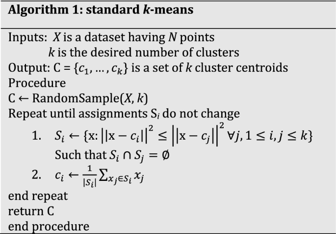
The goal of the k-means problem is to group N data points into k clusters, by finding a set of k centroids which minimize the sum of squared distances (SSD or SSE) between each point and its nearest centroid. A centroid is simply the center (mean) of points grouped together into one cluster. Thus, a k-means solution is uniquely defined by the set of k centroids. The standard k-means algorithm [38], also known as Lloyd’s algorithm, is a heuristic for approximating the solution to the problem. It starts by selecting k random points as the cluster centroids (initialization step), and each point is assigned to the nearest of these centroids. The centroid of each cluster is updated to be the mean of the points in that cluster (update step), after which the points are assigned again to the nearest updated centroid (assignment step). The update and assignment steps are repeated (iterations) until the assignment does not change (convergence). Franti and Sieranoja [30] identified as good reasons for k-means’ popularity, the fact that it is simple to implement and it is well understood. They emphasize the importance of simplicity in the choice of an algorithm. Fahim et al. [4] agree to the fact that k-means’ simplicity makes it widely favored, while also noting that k-means has been shown to produce good results in many applications. Other authors, such as [39], agree with these comments. Nevertheless, the algorithm is not without its shortcomings. Although k-means is efficient for small datasets, one major shortcoming is that its running time is proportional to data size and the number of clusters [4]. This becomes a problem in today’s age of massive datasets.

In this paper, we present an alternative approach to solving the k-means problem. Our approach scales well with data size. The approach is based on a generalization of the classical central limit theorem (CLT) from the single population case to the mixture distribution case. The classical CLT is a fundamental result in statistics and probability theory. It provides a basis for inferring population parameters from samples. It also provides a basis for applying methods meant for the normal distribution to arbitrary distributions. We discuss details of the theorem’s extension in Sect. 3. In our work, we observe that the classical CLT addresses a special case (k = 1) of the k-means problem, and then generalize it for all cases.

Two algorithms are presented to demonstrate the approach. In the first algorithm, named k-means-lite, instead of running k-means on the full dataset, a small sample is selected, k-means is applied to it and the centroids obtained are stored. This process is repeated a few (n) times. Finally, all the centroids obtained from all samples are combined into a new dataset (consisting of only nk points), to which k-means is now applied to obtain the final centroids. With sufficient number of samples (say 30 samples of size 40 +2k), this approach matches the performance of the standard approach in many cases and can even improve it in some cases. Additionally, the proposed approach addresses the local minimum problem that plagues the standard algorithm due to selection of multiple random samples. Experimental results presented in this paper also show that the results are also fairly accurate for this first algorithm, when only five samples are used. The key advantage, however, is that for a given choice of number and size of samples (which are easy to fix), the algorithm runs in constant time with respect to the data size.

The second algorithm presented in this paper, k-means-lite++, harnesses the advantage of seeding within our proposed framework. Specifically, in place of each run of k-means in k-means-lite, the k-means++ algorithm is used instead. The k-means++ algorithm uses D²-weighted sampling to choose initial centroids before running standard k-means. With this simple modification, the algorithm has speed that is still comparable to k-means-lite, and with only five samples, in many cases, it achieves accuracy that is superior to the standard k-means, matching that of the standard k-means++.

2 The standard k-means and k-means++ algorithms

To provide background for the rest of the study, we present brief descriptions of the standard k-means and k-means++ algorithms in this section.

2.1 The k-means algorithm

K-means partitions the data space into Voronoi cells [29]. In other words, given a dataset X in R^d, the goal of the k-means problem is to partition X into k groups (clusters) Y₁, Y₂, …, Y_k, such that ${\bigcup }_{i = 1}^{k} Y_{i} = X$ and $Y_{i} \cap Y_{j} = \emptyset$ for i ≠ j. Each cluster $Y_{i}$ is uniquely defined by a center $c_{i}$:

$$c_{i} = \frac{1}{{\left| {Y_{i} } \right|}}\mathop \sum \limits_{{y \in Y_{i} }} y.$$

Thus, a k-means solution is uniquely defined by the set of k centers $C = \left\{ {c_{1} , \ldots ,c_{k} } \right\}$. In optimization terms, the k-means objective is to find C so as to minimize the within-cluster variance $\emptyset$:

$$\phi = \mathop \sum \limits_{x \in X} \mathop {\hbox{min} }\limits_{c \in C} \left\| {x - c} \right\|^{2} .$$

The above sum-of-squares objective function is also referred to as distortion [40].

The k-means problem described above is NP-hard. The most popular heuristic for solving the problem is the Lloyd’s algorithm [40], popularly referred to, simply, as k-means algorithm. In this paper also, the term ‘k-means algorithm’ refers to this algorithm. The algorithm proceeds as follows:

• 1. Initialization: randomly select k data points to be used as an initial set of cluster centroids.

• 2. Repeat until assignment does not change:

  • (a) Assignment: Let each of the k centroids represent k different clusters, then assign each data point in the same cluster as its nearest centroid.

  • (b) Centroid update: For each cluster, update the centroid as the mean of all the points belonging to that cluster.

    

As earlier mentioned in Sect. 1, this algorithm is practical, effective and simple, but scales poorly, due to running time per iteration that is proportional to N and k. Furthermore, since initialization is random, the performance can also be arbitrary, a problem which k-means++ handles.

2.2 K-means++

Developed to address the sensitivity of the standard k-means algorithm to the choice of initial centroids, k-means++ is based on the intuition that the correct cluster centroids are well spread out, since they belong to different clusters. Thus, the k initial centroids are chosen such that they are far apart from each other. The k-means++ algorithm proceeds as follows [19]:

• 1. Randomly (uniform) select one data point to be used as one of the initial centroids.

• 2. Repeat until k centroids are chosen:

  • (a) For each data point, compute the distance $D^{2} \left( x \right)$ from the nearest of the already chosen centroids.

  • (b) Choose the next centroid c_i, selecting $c_{i} = x \in X$ with probability $\frac{{D^{2} \left( x \right)}}{{\mathop \sum \nolimits_{x \in X} D^{2} \left( x \right)}}$.

• 3. Proceed with standard k-means, initialized with the chosen centroids.

In Sect. 3, we highlight different approaches that have been adopted to improve the efficiency.

3 Related works

The k-means algorithm is dominated by computation of distances between each of k centroids and each of the N data points. This is done in every iteration. Thus, it computes Nk distances per iteration. So, its running time per iteration is O(Nk). The point is that k-means’ running time is proportional to N and k; thus, it grows fast with an increase in these values. Therefore, all solutions that have been proposed to address the problem are essentially techniques to reduce the number of distance computations performed. In this section, we briefly highlight approaches that have been adopted to achieve this goal.

3.1 Triangle inequality

Elkan [41] proposed a popular accelerated method which uses triangle inequality and tracking of point-to-centroid distance lower bounds, to avoid redundant distance computations. The algorithm yields same results as standard k-means. However, the costs of storing lower bounds may dominate in applications where k is large. Hamerly [42] builds on Elkan’s method by introducing a novel lower bound that allows the algorithm to eliminate k-means’ innermost loop 80% of the time in their reported experiments. Yet another improvement was proposed by Drake and Hammerly [43]. While Elkan’s method keeps k lower bounds and Hammerly’s method keeps one lower bound, this third algorithm employs an adaptive number b of stored lower bounds, such that 1 < b < k. The value of b is computed online. Agustsson et al. [44] proposed the k²-means algorithm which claims worst-case complexity of O(Nk_nd + k²d) and utilizes seeding and triangle inequality.

3.2 Kd-tree

Some efficient k-means extensions involve organizing the data into a kd-tree structure. The tree is traversed using a pruning test to reduce the number of distance calculations. Efficient kd-tree-based k-means algorithms include those of Alsabti et al. [45], Kanungo et al. [40] and Pelleg and Moore [46].

3.3 Sampling

Sampling is another approach that has been adopted to reduce k-means computational load. The general idea here is to reduce the number of distance computations by reducing the number data points used. Instead of dealing with the full data, methods in this category deal rather with samples. Sampling-based approaches include the method of Capo et al. [47] which partitions the full dataset recursively into a few subsets. It then applies a weighted k-means over representations of these subsets. Another notable work in this category is the mini-batch algorithm of Sculley [48].

3.4 Cluster closure

The method of Wang et al. [49] is based on the observation that most ‘active’ points that will change clusters are close to cluster boundaries. Active points are identified by pre-assembling the data into groups of neighboring points using multiple random spatial partition trees. The neighborhood information is used to construct a closure for each point. Thus, only those points in a centroids cluster closure need be considered during the k-means assignment step.

3.5 Seeding

In addition to these direct methods for reducing distance computations, efficiency has also been indirectly achieved through seeding. Although better efficiency is not always guaranteed, it has been reported in some studies [19, 50,51,52]. The point is that good initial centroids are likely to lead to faster convergence.

The approach proposed in this paper differs from many previous works, in that it does not modify the internal working of the standard algorithm. Rather, it is a ‘lightweight’ technique that ensures that the standard algorithm (or any other k-means clustering algorithm) is run on only a few very small samples. The power is in the fact that the standard algorithm is fast on small data. The proposed technique then uses statistical inference to compute the final solution for the full data from the outcome of these runs on the samples. We show that it is not only more wasteful to compute centroids using the full data, but can also be less accurate in some cases. Since the main focus of this paper is to address k-means’ scalability problem, one interesting attribute of our method is that the running time is not a function of data size, for a given combination of number and size of samples (which are easy to fix). Two algorithms are presented to demonstrate our proposed approach: one based on k-means and the other on k-means++ [19]. The k-means++ algorithm, widely considered the state-of-the-art algorithm within the k-means family, was proposed to solve another k-means problem: sensitivity to the choice of initial centroids. K-means’ sensitivity to the choice of initial centroids, which creates accuracy problems, is addressed by incorporating a seeding module into the standard algorithm. Instead of random selection, seeding methods pick initial centroids systematically. K-mean++ is well-studied and widely used. It employs the state-of-the-art D²-weighted sampling proposed independently by Arthur and Vassilvitski [19] and Ostrovsky et al. [53]. K-means++ has been shown in [19] to provide accuracy guarantee, being O(log k)-competitive. However, its sequential nature makes it time-consuming for large datasets [54]. This means the seeding method of k-means++ also suffers from poor scalability. Hence, some authors have resorted to approximations such as the approximate k-means++ method of Bachem et al. [54] and the related method of [55]. K-means-lite++, our second algorithm, can be seen as a more scalable version of k-means++.

In summary, our paper presents a constant-time k-means clustering approach based on statistical inference of population centroids from the centroids obtained from independent samples. In Sect. 4, we show that the classical central limit theorem addresses a special case (k = 1) of the k-means problem. Then, we generalize to all cases, leading to a simple algorithm, named k-means-lite. The approach is fast, accurate and free from k-means’ local optimum problem. In Sect. 4, we present analyses related to performance guarantees for k-means-lite. In Sect. 5, we discuss the k-means-lite++ algorithm, a modification of k-means-lite, in which we replace every appearance of k-means in k-means-lite with k-means++. After these, experimental results are presented comparing the new algorithms with their traditional counterparts, to establish the value of the proposed approach.

4 The proposed k-means-lite paradigm

In this section, we describe the proposed clustering approach. We begin by discussing the theoretical basis and then describe the proposed k-means-lite algorithm and its improved version, k-means-lite++.

4.1 The central limit theorem (CLT) and estimation of population mean

The CLT is widely regarded as one of the most central results of probability theory. It has a long history and exists in various forms with diverse proofs. Trotter presented an elementary proof in [56]. Two proofs are discussed in Filmus’ work [57]. History and concepts of the CLT are extensively discussed by Fischer [58], Mether [59], Le Cam [60] and Adams [61]. In brief, suppose {x₁, x₂, …, x_|S|} is a sequence of independently and identically distributed (i.i.d) random variables having expected value $E\left[ x \right] = \mu$ and finite variance ${\text{Var}}\left[ x \right] = \sigma^{2}$. The CLT states that as $\left| S \right|,n \to \infty$, $\left| S \right|\mathop \to \limits^{d} N\left( {\mu ,\sigma^{2} /\left| S \right|} \right)$,where $\overline{S} \text{ := }\frac{{x_{1} + \cdots + x_{\left| S \right|} }}{\left| S \right|}$. In other words, if from an arbitrarily distributed population that has mean $\mu$ and variance $\sigma^{2}$, we select independent random samples n times and obtain each sample mean $\overline{S}_{1} , \ldots , \overline{S}_{n}$, for sufficiently large n, the distribution of these sample means is (approximately) a normal distribution with mean $\mu$ and variance $\sigma^{2} /\left| S \right|$. One application of this theorem, related to our study, is that the mean of a sequence of numbers can be accurately estimated without adopting the traditional approach that involves dealing exhaustively with all the numbers.

As a toy example to illustrate this application, suppose we want to find the mean of the set {1, 2, 3, 4, 5}, the traditional approach yields (1 + 2 + 3 + 4 + 5)/5 = 3. Now, let us apply the CLT-based method. With the aid of a computing software, we select three numbers randomly, three different times. The first sampling yields the subset {4, 1, 3}, the second yields {1, 2, 5} and the third {5, 4, 2}. The means of the samples are 2.6667, 2.6667, and 3.6667, respectively. The mean of these means is (2.6667 + 2.6667 + 3.6667)/3 = 3.0000. A second trial of this method yields samples, {4, 5, 3} , {1, 3, 4} and {5, 1, 4}, which have means 4.0000, 2.6667 and 3.3333, respectively, and a final answer (4.0000 + 2.6667 + 3.3333)/3 = 3.3333. This is still close to the true mean. Notice the final answer obtained by taking the mean of samples estimates the true population mean more accurately than individual sample means. This shows the advantage of the CLT-based approach over uniform sampling. We discuss this advantage in more detail in Sect. 5.

We present another example that further reveals the behavior of this CLT-based method. We want to find the mean of {1, 2, …,1000} using different combinations of sample sizes and number of samples. We do not bother to report the sample means, but only the final results. The experiment is repeated for each combination 30 times, and average result over these 30 runs is reported in Table 1.

Table 1 Performance of the CLT-based method for computing the mean of a set of numbers

We note in the given examples that the CLT-based approach is able to produce good results using a few samples. Now, if we fix the number and size of sample (to values that work well for most problems), then the method takes the same amount of time for all problems, regardless of data size. In order words, it is highly scalable. Precisely, it runs in constant time with respect to data size. Another observation is that although the direct method is faster for small datasets, the CLT method continues to gain efficiency over the direct method, as data size increases.

4.2 The CLT and k-means clustering, for k = 1

A key observation of our work is that the problem of finding the mean of a given set of numbers is equivalent to a special case of the k-means clustering problem, where k = 1. The goal of the k-means problem for this case is to find the single centroid (mean) of an entire set of points in R^d. Three different ways to achieve this are as follows:

• 1. The direct method: Perform vector addition of all the data points and divide the result by the number of points.

• 2. The standard k-means algorithm (Lloyd’s method): Select a point at random to be used as the initial centroid. Then, assign each data point to its nearest centroid. In this case, all points get assigned to the single centroid. Finally, compute the mean of all the points assigned to this centroid. This last step which obtains the final centroids is identical with the direct method.

• 3. CLT-based method (k-means-lite): Select a sample of size of s, apply the standard k-means to this sample and store the centroid (mean) of this sample. Repeat this process until n samples have been selected. Combine the n centroids into a single set of points and apply standard k-means to this combination to obtain the final mean. Note than any mean finding method (such as the direct method) can replace k-means in the described framework. The value of this framework will lie in its ability to ensure that the base method is only applied to small data (sufficiently small s) and is only run a few times (sufficiently small n). In this way, when the dataset is very large, the algorithm’s running time does not change much. Note also that the samples are i.i.d; that is, the points selected in a previous sample ‘have been returned’ back to the original dataset before another sample is selected. This distinguishes k-means-lite from mere divide-and-conquer strategy. Independence of samples is required for CLT to hold.

The third method explains how k-means-lite works. We generalize the method to the any k in the next subsection (Sect. 4.3), to have our k-means-lite algorithm.

4.3 Generalizing the CLT for k-means clustering

The key to generalizing from the k = 1 case to all k lies in recognizing the dataset as a mixture of k different distributions. Hence, the standard algorithm starts with k centroids, so that the points are clustered into k groups. Our proposed k-means-lite algorithm remains as described for the k = 1 case in Sect. 4.3 (method 3). It is the k-means component that needs to cater for the change in k. In other words, each time a sample is selected from the dataset, that sample is partitioned into k clusters and k centroids are obtained. After all n samples have been selected, there will be a total of nk centroids forming a new dataset, to which k-means is again applied to obtain the final k centroids. Before presenting our extension of the CLT for the general k-means problem, we establish that (with high probability) a sufficiently sized sample contains points from all clusters and for sufficiently large n, the average proportion within the sample occupied by points belonging to any given cluster u approaches the expected proportion |u|/N. This makes it almost impossible for our algorithm to miss a cluster. This validates our extension to the CLT and also establishes the reliability of k-means-lite.

Lemma 1

[62] For a cluster A, if the sample size s satisfies

$$s \ge\, fN + \frac{N}{\left| A \right|}\log \left( {\frac{1}{t}} \right) + \frac{N}{\left| A \right|}\sqrt {\left( {{ \log }\left( {\frac{1}{t}} \right)} \right)^{2} + 2f\left| u \right|{ \log }\left( {\frac{1}{t}} \right)}$$

Then, the probability that the sample contains fewer than f|A| points belonging to cluster A is less than $t , 0 \le t \le 1$.

Guha et al. [62] presented the above lemma and concluded based on the inequality that for a sample to contain at least f|A| points that are from a cluster A with high probability, the sample should have more than a fraction f of N. They also observe that the inequality holds for the minimum-sized cluster A_min, and if s_min is the result of substituting A_min for A in the inequality, the probability that the number of points selected from any cluster A is fewer than f|A| has an upper bound of $kt$.

Lemma 2 provides more insight on s and the probability of missing a cluster.

Lemma 2

$\lim_{s \to \infty } \Pr \left[ {A \cap S = \emptyset } \right] = 0$, where $S$ is a random sample selected from X, $A$ is an arbitrary cluster in X, $s = \left| S \right|$ and $\emptyset$ is the empty set.

Proof

The lemma follows from Lemma 1. If s (the left-hand side of the inequality) is increased, f is increased as well. So, as $s \to \infty$, $f \to 1$. Now,

$$f = \frac{{\left| {A \cap S} \right|}}{\left| A \right|}$$

$$\left| {A \cap S} \right| = \left| A \right|f.$$

Clearly, as $s \to \infty$, which causes $f \to 1$, $A \cap S \to A \ne \emptyset$ and $\mathop {\lim }\nolimits_{s \to \infty } { \Pr }\left[ {A \cap S = \emptyset } \right]$ goes to 0.□

Practically, Lemma 1 means that if s is sufficiently large (s ≫ k), it is unlikely that the sample will not contain at least a few points from every cluster. This fact is a necessary foundation for our extended CLT. We discuss more about choosing an appropriate value for s in Sect. 5 (Theorem 5).

Lemma 3

$\mathop {\lim }\nolimits_{n \to \infty } \overline{p} = \frac{\left| A \right|}{N}$ and $\mathop {\lim }\nolimits_{n \to \infty } {\text{Var}}\left[ p \right] = \frac{\left| A \right|}{N}\left( {1 - \frac{\left| A \right|}{N}} \right)$ where $p_{i}$ is the random variable defined as $p_{i} = \frac{{\left| {A \cap S_{j} } \right|}}{s}, \quad j \in \left\{ {1, \ldots ,n} \right\}$.

Proof

Let $p_{i}$ be the proportion of points from an arbitrary cluster u, in the sample $S_{j} :j = 1, \ldots ,n$.The event of selecting a point from cluster A constitutes a Bernoulli trial. Given s ≪ N (small sample from a large population), the selections of each point in a given sample are practically independent, and the number of successes (picking from cluster A). Thus, $\Pr \left[ {\text{success}} \right] = \left| A \right|/N$. Therefore, mean number of successes is $\frac{s\left| A \right|}{N}$ and the variance is $\frac{s\left| A \right|}{N}\left( {1 - \frac{\left| A \right|}{N}} \right)$ yielding mean and variance of proportions of $\frac{\left| A \right|}{N}$ and $\frac{\left| A \right|}{N}\left( {1 - \frac{\left| A \right|}{N}} \right)$, respectively. Thus, $E\left[ p \right] = \left| A \right|/N$. This is also consistent with the law of large numbers. Now,

$$p = \frac{{p_{i} + \cdots + p_{n} }}{n}$$

$$E\left[ p \right] = \frac{{E\left[ {p_{i} } \right] + \cdots + E[p_{n} ]}}{n} = \frac{nE\left[ p \right]}{n}$$

$$E\left[ p \right] = \mathop {\lim }\limits_{n \to \infty } p = E\left[ p \right] = \frac{\left| A \right|}{N}.$$

Lemma 2 is nothing but a manifestation of the CLT, which applies not only to distribution of sample means but also to that of sample proportions. Both are specific cases of normalized sums of i.i.d. random variables. So, we know that as $n \to \infty$, $p_{i} \mathop \to \limits^{d} N\left( {\frac{\left| A \right|}{N},\frac{1}{n}\frac{\left| A \right|}{N}\left( {1 - \frac{\left| A \right|}{N}} \right)} \right)$, and the distribution of sample proportions approaches Gaussian with mean $E\left[ p \right]$ (equal to the true population proportion).□

Practically, Lemmas 1 and 2 imply that, provided s ≫ k, for each cluster A, every sample of size s will contain points from A (with high probability), and the number of points of a cluster A contained in the sample fluctuates (approximately normally distributed) around $\frac{\left| A \right|}{N}s$ with finite variance $\frac{s\left| A \right|}{N}\left( {1 - \frac{\left| A \right|}{N}} \right)$. We illustrate the concept further with an empirical example. We take the G2-2-20 dataset [30] which has N = 2048 points and k = 2 clusters. Each cluster covers 50% of the entire data (1024 points each). We select random samples of varying sizes $s \in \left\{ {10,20,30,40,50,100} \right\}$. For each sample size s, we perform 1000 trials and record the average proportion of each cluster in each sample selected.

$${\text{Proportion }}p_{j} {\text{ for cluster }}j = \, \left| {{\text{selected cluster }}j{\text{ points}}} \right|/s$$

The results in Table 2 validate Lemmas 1 and 2, showing that the mean of sample proportion for a given cluster u approaches |u|/N as more samples are used. Figure 1 shows further detail: the distribution of the sample proportion over the 1000 trials, for each sample size.

Table 2 G2-2-20 dataset: average proportion of points from each cluster in 1000 random samples

Fig. 1

Distribution of sample proportions for points belonging to cluster 1 over 1000 trials (sample size = 100) is bell-shaped, i.e., normal, with mean ≈ 0.5 (the proportion the cluster occupies in the full dataset)

Now, we proceed to generalize the CLT. We note that the k-means clustering problem is a generalization of the problem of finding the mean of a single distribution. Precisely, it can be viewed as the process of simultaneously finding the mean of each of the k components in a mixture distribution. We have shown earlier how the classical CLT provides a scalable method for solving the special case k = 1. Our goal here is to generalize this CLT-based method, which becomes a scalable k-means clustering method.

Theorem 1

(Generalized Central Limit Theorem for Mixture Distributions) Given $S_{j} = \left\{ {x_{1} , \ldots ,x_{s} } \right\},\quad j \in \left\{ {1, \ldots ,n} \right\}$ which is a sequence of independently and identically distributed (i.i.d) random variables, $\forall i \in \left\{ {1, \ldots ,k} \right\}, \quad \hat{\mu }_{i} \mathop \to \limits^{d} N\left( {\mu_{i} ,\frac{{\sigma^{2}_{i} }}{{s_{i} }}} \right)$, as $n,s_{i} \to \infty$, where $\widehat{\mu }_{i} : = \frac{{\sum \left( {S_{j} \cap A_{i} } \right)}}{{|S_{j} \cap A_{i} |}}$, $s_{i} \le {\text{s}}$ is the number of points picked from $A_{i}$ the $i$th component of a mixture of k distributions, with $E\left[ {A_{i} } \right] = \mu_{i}$ and ${\text{Var}}\left[ {A_{i} } \right] = \sigma_{i}^{2}$.

Proof

The theorem follows from Lemmas 1 and 2. Lemma 1 establishes that each sample of sufficient size s ≫ k will contain points from each cluster (with high probability). This probability approaches 1 as s increased. Consequently, each sample $S_{j}$ of size s selected from a mixture of k distributions $A_{1} , \ldots ,A_{k}$ is itself a mixture having k components $S_{j} \cap u_{1} , \ldots ,S_{j} \cap A_{k}$, and the mean $\hat{\mu }_{i}$ of the $i$ th component of $S_{j}$ is given by $\hat{\mu }_{i} : = \frac{{\sum \left( {S_{j} \cap A_{i} } \right)}}{{\left| {S_{j} \cap A_{i} } \right|}}$.Since $\hat{\mu }_{i}$ is the random variable constructed by taking the mean of points sampled from $A_{\alpha }$, then each pair of $\hat{\mu }_{i}$ and $A_{i}$ is related by the classical CLT. Therefore, as $n,s_{i} \to \infty , \quad \hat{c}_{i} \mathop \to \limits^{d} N\left( {\mu_{i} ,\frac{{\sigma^{2}_{i} }}{{s_{i} }}} \right)$□

4.4 The k-means-lite algorithm

In clustering terms, we recast Theorem 1; thus, given a dataset X which consists of k clusters having centroids $\mu_{1} , \ldots , \mu_{k}$, if n random samples are taken from P, and each is partitioned into k clusters, each defined by k centroids, then the k centroids obtained by partitioning the collection C of sample centroids into k clusters approach $\mu_{1} , \ldots , \mu_{k}$, as the number of samples and size of samples are increased. Also, C consists of k clusters that are denser and better separated (within-cluster variance lowered by a factor of equal to the sample size) than the clusters in the original dataset. Our proposed k-means-lite is explained by these insights. The algorithm is outlined as follows:

Input: dataset X, number of clusters k, sample size s, number of samples n.

• 1. Repeat n times:

  • (a) Select a sample of size s from the dataset.

  • (b) Run standard k-means algorithm on the sample and store the centroids.

• 2. Obtain the optimal centroids by running k-means on the combination of the stored centroids.

• 3. Assign each point in X to the nearest centroid in C.

  

5 Analysis

This section presents some useful analysis of k-means-lite. Specifically, we focus on time complexity and approximation bound. The latter establishes theoretical comparison of the performance of k-means-lite with the full-data version, as well as with ordinary uniform sampling. Throughout this section, the term Q-lite describes the scaled version of any k-means algorithm Q.

5.1 Complexity

As a key result of this paper, we present Theorem 2, showing the time complexity is constant in the number of data points.

Theorem 2

K-means-lite’s running time is O(1) in N.

Proof

The algorithm selects n samples each of size s, clusters each with k-means to obtain a collection of nk centroids which is clustered, again using k-means, to obtain the final k centroids. Let t be the number of k-means iterations that a sample will take, and let T be the number of iterations, if k-means were run on the full dataset. Clustering each sample takes O(skt); that is, in each of the t iterations, k centroids are compared, to make a total of O(nskt + nk²t) or O((ns + nk)kt). Clearly, the complexity is not a function of N, unlike k-means’ complexity of O(NkT).□

The result of the above complexity analysis has the following implications:

• 1. As mentioned, k-means-lite’s running time is not a function of data size.

• 2. Although k-means-lite will always be fast (less than 1 s on the average computer for the many well-known datasets), k-means could be faster when N is small enough for t ≈T and (ns + nk) > N.

• 3. As N is increased, k-means running time grows proportionately, while k-means-lite should be able to maintain roughly the same running time, if s and n are fixed.

5.2 Performance bound

Here, we are concerned with accuracy guarantees offered by the proposed approach. We present the well-known Lemma 4, which is foundational to our analysis [19, 63, 64].

Lemma 4

$$\phi_{{Q} \left( A \right) }- \phi_{{\text{OPT}}} \left( A \right) = \left| A \right|.\left| {\left| {\hat{\mu }_{QA} - \mu } \right|} \right|^{2}$$

where $\phi \left( A \right)$ is the SSE computed by an algorithm on a cluster A, $\phi_{{\text{OPT}}} \left( {\text{A}} \right)$ is the optimal solution and $\hat{\mu }_{QA}$ and $\mu$ are the estimated and optimal centers for A, respectively.

Theorem 3

Given an exact algorithm Q, that is, $\Delta_{QA} = \left| {\hat{\mu }_{QA} - \mu } \right|$ = 0 then, Q-lite is asymptotically exact, that is, $\Delta_{\text{Qlite}} = \left| {\hat{\mu }_{\text{Qlite}} - \mu } \right|$  ≈ 0, for sufficient n and a.

Proof

Let $\Delta_{QA} = \left| {\hat{\mu }_{QA} - \mu } \right|$ be the deviation of the center estimate $\hat{\mu }_{QA}$ produced by Q when applied to the full cluster. If Q is exact ($\Delta_{QA} = 0$), then if it is applied to a sample a instead, by the CLT, the deviation $\Delta_{Qa} = \left| {c - \mu } \right|$ is given by the random variable:

$$\Delta_{Qac\mu } = \frac{{z\sigma_{A} }}{{\sqrt {\left| a \right|} }}$$

where z ~ N(0,1). So,

$$\Delta_{Qac\mu } \le \frac{{z_{ \propto } \sigma_{A} }}{{\sqrt {\left| a \right|} }}$$

Intuitively, this means (100 − $z_{ \propto }$) % of the time, $c$ is within a distance of $\frac{{z_{ \propto } \sigma_{A} }}{{\sqrt {\left| a \right|} }}$ from $\mu$. We can take $z_{ \propto } = 3$ (99.7% confidence) as a reasonable conclusion.

The corresponding deviation $\Delta_{Qa}$ produced by Q-lite is:

$$\Delta_{\text{Qlite}} = E\left( {\Delta_{Qa} } \right) = E\left( {\frac{{z\sigma_{A} }}{{\sqrt {\left| a \right|} }}} \right) = \frac{{\sigma_{A} }}{{\sqrt {\left| a \right|} }}E\left[ z \right] = 0.$$

That is, unlike ordinary sampling, despite Q-lite’s improvement of Q’s time complexity, it is asymptotically exact, if Q is exact: the general case in which Q may be only able to produce an approximate solution.

Theorem 4

Given $\phi_{Q} \left( A \right) \le \phi_{\text{OPT}} \left( A \right) + \Delta_{QA}^{2} \left| A \right|$, then $\phi_{\text{Qlite}} \left( A \right) \le \phi_{\text{OPT}} \left( A \right) + \left( {1.2-\delta} \right)^{2} \Delta_{QA}^{2} \left| A \right|$, where $\delta$ is a small constant.

Proof

Now, we consider the general case, where Q is itself an approximate clustering algorithm, as is the case with all practical algorithms.Take Q to be a β-approximation algorithm: for any cluster A, $\phi_{Q} \left( A \right) \le \beta \phi_{\text{OPT}} \left( A \right)$. The deviation of the estimated cluster center comes from two sources: approximation error and sampling error. By Lemma 4, $\phi_{Q} \left( A \right) = \phi_{\text{OPT}} \left( A \right) + \left( {\beta - 1} \right)\phi_{\text{OPT}} \left( A \right)$. Similarly, $\phi_{Q} \left( a \right) = \phi_{\text{OPT}} \left( a \right) + \left( {\beta - 1} \right)\phi_{\text{OPT}} \left( a \right)$. Thus,

$$\beta - 1 = \frac{{\Delta_{QA}^{2} \left| A \right|}}{{\phi_{\text{OPT}} \left( A \right)}} = \frac{{\Delta_{Qa}^{2} \left| a \right|}}{{\phi_{\text{OPT}} \left( a \right)}}$$

$$\frac{{\Delta_{Qa}^{2} }}{{\Delta_{QA}^{2} }} = \frac{{\left| A \right|\phi_{\text{OPT}} \left( a \right)}}{{\left| a \right|\phi_{\text{OPT}} \left( A \right)}} = \frac{{\left( {\left| a \right| - 1} \right)\sigma_{a}^{2} }}{{\left| a \right|\sigma_{A}^{2} }}$$

$$\Delta_{Qa} = \frac{{\Delta_{QA} \sigma_{a} }}{{\sigma_{A} }}\sqrt {\frac{\left| a \right| - 1}{\left| a \right|}} .$$

$\Delta_{Qa}$ is the deviation of the estimated sample center $c_{a}$ from the true sample center $\hat{\mu }_{a}$. Thus, the total distance from $c_{a}$ to $\mu$ is:

$$\Delta_{Qac\mu } = \Delta_{Qa} + \frac{{z\sigma_{A} }}{{\sqrt {\left| a \right|} }} = \frac{{\Delta_{Qa} \sigma_{a} }}{{\sigma_{A} }}\sqrt {\frac{\left| a \right| - 1}{\left| a \right|}} + \frac{{z\sigma_{A} }}{{\sqrt {\left| a \right|} }}$$

$$\Delta_{Qac\mu } \le \frac{{\Delta_{QA} \sigma_{a} }}{{\sigma_{A} }}\sqrt {\frac{\left| a \right| - 1}{\left| a \right|}} + \frac{{z_{ \propto } \sigma_{A} }}{{\sqrt {\left| a \right|} }}$$

Now, if we select several samples and collect the estimated sample centers, into a single dataset $\overline{c}$, then the true center of $\overline{c}$ deviates from $\mu$ by $\Delta_{{{\text{OPT}},\bar{c}}}$:

$$\Delta_{{{\text{OPT}},\overline{c} }} \le E\left[ {\Delta_{Qac\mu } } \right] = E\left[ {\frac{{\Delta_{QA} \sigma_{a} }}{{\sigma_{A} }}\sqrt {\frac{\left| a \right| - 1}{\left| a \right|}} + \frac{{z\sigma_{A} }}{{\sqrt {\left| a \right|} }}} \right] = g\left( a \right)\Delta_{QA} \sqrt {\frac{\left| a \right| - 1}{\left| a \right|}}$$

where

$$g\left( {\left| a \right|} \right) = \sqrt {\frac{2}{\left| a \right| - 1}} \frac{{\varGamma \left( {\frac{\left| a \right|}{2}} \right)}}{{\varGamma \left( {\frac{\left| a \right| - 1}{2}} \right)}} = 1 - \frac{1}{4\left| a \right|} - \frac{7}{{32\left| a \right|^{2} }} - \frac{19}{{128\left| a \right|^{3} }} + O\left( {\left| a \right|^{ - 4} } \right)$$

where $\varGamma \left( . \right)$ is the gamma function. The total deviation of Q-lite’s estimated center from the true cluster center $\Delta_{\text{Qlite}} = \left| {\hat{\mu }_{\text{Qlite}} - \mu } \right|$

$$\Delta_{Qlite} \le g\left( a \right)\Delta_{QA} \sqrt {\frac{\left| a \right| - 1}{\left| a \right|}} + {\Delta_{{Q\bar{c}}} }\sqrt {\frac{n - 1}{n}} .\frac{{\sigma_{{\bar{c}}} }}{{\sigma_{A} }}$$

where $\Delta_{{Q\overline{c} }}$ is the worst deviation Q produces on $\bar{c}$. For sufficient n and a, by the CLT, $\sigma_{{\overline{c} }} \to \frac{{\sigma_{A} }}{{\sqrt {\left| a \right|} }}$, and $\bar{c}$ approaches normal distribution and is denser than A, which implies better clusterability. So, $\frac{{\Delta_{{Q\bar{c}}} }}{{\Delta_{QA}}} = \frac{1}{\gamma } < 1$.

$$\begin{aligned} \Delta_{\text{Qlite}} &\le \frac{{\Delta_{QA} }}{{\sqrt {\left| a \right|} }}\left( {g\left( a \right)\sqrt {\left| a \right| - 1} + \frac{1}{\gamma }\sqrt {\frac{n - 1}{n}} } \right) \hfill \\ \Delta_{\text{Qlite}} &\le \left( {1 + \epsilon } \right) \Delta_{QA} , \hfill \\ \end{aligned}$$

if we take $\frac{1}{\gamma }=1, \left( {1 + \epsilon } \right) < 1.2$. And the theorem follows.□

5.3 Advantage over simple uniform sampling and repeated sampling

We briefly highlight a few points in our analysis that establish the advantage of our approach compared to ordinary uniform sampling. Sampling is perhaps one of the most effective ways to gain efficiency. But the more the gain in efficiency (achieved by reducing the sample size), the worse the performance. One way to improve the performance of sampling is to increase the sample size, but this defeats the purpose of sampling. If the algorithm could handle large data fast, there will be no need for sampling in the first place. K-means-lite provides a more efficient solution. Since we know $E\left[ {\mu_{a}^{2} } \right] = \mu_{A}^{2}$, then if we take the mean of the sample center estimates, we can recover the true mean with high precision. Notice in the exact case, where Q produces the true solution, uniform sampling does not. It can deviate from the true solution as far as $\Delta_{Qac\mu } \le \frac{{z_{ \propto } \sigma_{A} }}{{\sqrt {\left| a \right|} }}$ and as far as $\Delta_{Qac\mu } \le \frac{{\Delta_{QA} \sigma_{a} }}{{\sigma_{A} }}\sqrt {\frac{\left| a \right| - 1}{\left| a \right|}} + \frac{{z_{ \propto } \sigma_{A} }}{{\sqrt {\left| a \right|} }}$ in the approximate case (such as the k-means algorithms we seek to improve). Our ‘lite’ approach takes advantage of the CLT to correct this error by computing the expected value of each component. The $\frac{{z\sigma_{A} }}{{\sqrt {\left| a \right|} }}$ component, therefore, is corrected to zero, while the first component is corrected to the mean $g\left( a \right)\Delta_{QA} \sqrt {\frac{\left| a \right| - 1}{\left| a \right|}}$, with a small approximation error introduced depending on the quality of the algorithm. If uniform sampling is repeated several times, so that the best is chosen, with sufficient trials, very good results will be obtained, with high probability. One disadvantage of such an approach is that time only saved in computing centroids; typically (as in the CLARA [65] algorithm which uses repeated sampling to improve the efficiency of k-medoids), each of the centroids set obtained from samples is evaluated over the full dataset. In our approach, these evaluations are unnecessary. Our approach provides better guarantee, as shown in the analysis. We also show via brief experiments that the proposed approach produces better results.

5.4 Brief experiment: comparing single and repeated uniform sampling with the proposed approach

We compare the performance of k-means-lite (with 30 samples) and k-means applied to uniform sample. We also study the effect of applying k-means on multiple (30 samples) and then choosing the solution (centroids) that yields the lowest cost over the full data. We employ the same settings to k-means++. Table 3 shows the accuracies achieved by each method, based on Adjusted Rand Index (ARI). Table 4 compares accuracy based on k-means cost (SSE). As Tables 3 and 4 show, there is no single case among the five cases tested, in which our approach does not outperform sampling (single or repeated). This is true for both the k-means and k-means++ versions of these methods. Moreover, repeated sampling is less efficient (Table 5). This is due to the computation of distances between each sample centroid set and the full data, to evaluate the quality of each solution. This makes the running time a function of N. Our approach, on the other hand, does not evaluate each sample centroid set, but only clusters their combination.

Table 3 Comparing k-means-lite with uniform sampling: ARI (%)

Table 4 Comparing k-means-lite with uniform sampling: SSE

Table 5 Comparing k-means-lite with uniform sampling: running time (s)

5.5 Highlights of advantages of k-means-lite compared to the conventional approach

Besides comparison with traditional sampling, we note the following advantages of our proposed approach over the conventional full-data approach.

• 1. Since the number and size of samples can be fixed to values that generally work well, with these fixed values, the algorithm runs in constant time, with respect to data size. That is, the running time is not a function of the data size. This implies that the algorithm is highly scalable.

• 2. The algorithm consists of n + 1 runs of standard k-means, each on very small data. The last of these n + 1 runs is typically performed on much smaller and ‘nicely’ clustered data. Since the standard k-means algorithm is fast for small data, k-means-lite’s speed is ensured on small and large data.

• 3. The k-means-lite algorithm can be viewed as a process of mapping a large dataset to a small derived dataset (the combination of sample centroids), which can be used to accurately find the solution without dealing with the full dataset. Although small in size, this derived dataset possesses the following properties:

  • (a) It shares similar cluster structure and cluster centers, with the full dataset.

  • (b) Its clusters are (approximately) Gaussian.

  • (c) Its clusters are denser than those in the original data.

These properties are ‘nice’ properties for clustering algorithms, and they lie at the root of k-means-lite’s effectiveness. Illustrating these properties, Fig. 2b shows the derived dataset constructed from the G2-2-20 dataset (Fig. 2a).

Fig. 2

a Original data: g2-2-20 (2048 points). b k-means-lite illustrated: top left to bottom right: centroids set derived using 1, 2, 3, 4, 5, 20, 30, and 1000 random samples of 40 + 2 k. Notice how the derived dataset has neatly separated, dense clusters that are representative of the original data cluster structure

• 4. As an added advantage, k-means-lite addresses k-means’ problem of local optima, due to the use of multiple samples, which introduces better randomization.

• (5) Unlike many existing approaches to improving k-means efficiency, we have made no changes to the k-means algorithm itself. Rather, k-means-lite is a framework wrapped around the algorithm, using it to infer the solution from samples. Thus, the proposed approach can be used to scale any other k-means clustering algorithm.

• 6. Depending on the specific algorithm used in clustering the samples, it is asymptotically possible to achieve the true (globally optimal) clustering for any given problem. This will be achieved if the base algorithm is sufficiently accurate on the samples and the number and size of samples are large enough, so that $S^{\left( \alpha \right)} - \mu_{\alpha } < e$, where e is the maximum perturbation allowed for $\mu_{\alpha }$, to retain the true clustering.

5.6 Choosing number and size of samples

There are two questions that arise in the implementation of k-means-lite. Firstly, how many points should be selected to make a sample? Secondly, how many samples should be selected?

Since we have established that, assuming the ‘right’ sample size and number of samples, the sample mean comes from an (approximately) Gaussian distribution with mean equal to the true centroid. With this information, if we were seeking to fit the entire Gaussian distribution, we will need a high number of large samples, but since the goal is to locate the population mean (which converges much faster than the tails), a few small samples should suffice (Fig. 3).

Fig. 3

2-D plots of some synthetic datasets studied (one member per group). From top left to bottom right: A1, S1, Dim256, Birch1, Birch 2, Iris, C5k1mN

For the implementation presented in this paper, we go with convention established for the popular CLARA k-medoids algorithm, which is also a sampling-based clustering algorithm. Although not in the k-means family, k-medoids also seeks k centers. CLARA runs k-medoids on multiple (say 5) samples of 40 + 2k [65, 66] and chooses the best k centers (most central data points, not centroids) evaluated over the full dataset. Since this algorithm is successful and well known, we reckon that its settings can be adopted in our approach; especially the sample size. We further justify this choice of sample size 40 + 2k by Theorem 5.

Theorem 5

If s ≥ 2k, then, E[ψ] ≥ 2, provided clusters are uniform, where ψ is the number of points picked from an arbitrary cluster. For non-uniform clusters, provided probability of picking a point from that cluster is $p \ge {\raise0.7ex\hbox{$1$} \!\mathord{\left/ {\vphantom {1 {2k}}}\right.\kern-0pt} \!\lower0.7ex\hbox{${2k}$}}$, s ≥ 2k yields E[ψ] ≥ 1.

Proof

Uniform clusters, an assumption of the k-means formulation, imply $p = 1/k$.Also, with sample size s ≪ N, the selection of points to make up a sample is practically independent. So, expected number of hits E[ψ] for that cluster = s/k. Consider three possible cases. One, if s < k, then E[ψ] = 0; two, s = k, then E[ψ] = exactly 1, requiring the impractical condition that p be strictly 1/k; lastly, s ≥ 2k, then E[ψ] ≥ 2. Clearly, s ≥ 2k should be satisfied. With this choice, E[ψ] ≥ 1 still holds, as long as $p \ge \frac{1}{2k}$. This second part follows from $E\left[ {{\psi }} \right] = sp \ge \frac{s}{2k}$, and the second part of the theorem follows.□

The choice of 40 + 2k points is therefore sound. With E[ψ] > 1, then we expect this setting applied to our algorithms, to give reasonably accurate results, while selecting up to 30 samples is expected to yield algorithms with performance very close to the theoretical guarantees.

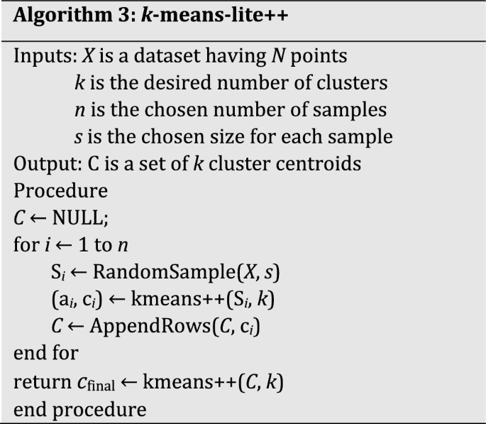
6 K-means-lite++: the advantage of per-sample seeding

We identify an opportunity to improve the proposed k-means-lite algorithm, by employing the D ²-weighting-based seeding of k-means++ for each k-means-lite sample. Basically, we replace every k-means run in k-means-lite with k-means++. With this simple modification, experimental results (in Sect. 7) show that the resulting algorithm, k-means-lite++, is nearly as efficient as k-means-lite and statistically indistinguishable from the state-of-the-art algorithm, k-means++ (more accurate than k-means), if only five samples are used. With 30 samples, k-means-lite++ even surpasses the accuracy of k-means++.

The accuracy and efficiency of k-means-lite++ can be explained by two factors. First, high accuracy is expected because k-means++ provides better accuracy guarantees than k-means. Thus, the quality of the derived dataset from which the final centroids are obtained will be improved if it was constructed using k-means++ on each sample, in place of k-means. Second, high efficiency/scalability is expected because the k-means++ component of our algorithm is never run on large data throughout. This is because, typically, k is less than a few hundreds even in cases that would be considered very large. In many applications, even when N is large (millions or hundreds of thousands), k might even be less than 10. So, for our samples of size 40 + 2k and the derived dataset C which has size of 5 k (if 5 samples are used) or 30 k (if 30 samples are used), the poor scalability of k-means++’s seeding technique pointed out by Bachem et al. [54] is not an issue.

In summary, the proposed k-means-lite++ algorithm is outlined as follows (see pseudocode in Algorithm 3):

• 1. Select n samples, each of size s from the dataset P.

• 2. Run k-means++ on each sample and store the cluster centroids in C (size nk).

• 3. Run k-means++ on C to obtain the final centroids set.

• 4. Assign each point in P to the nearest medoid in c_final.

  

7 Experiments

To evaluate the proposed clustering approach, we compare the speed and accuracy of our algorithms against those of their traditional counterparts, k–means and k-means++. Speed is measured by CPU time, while accuracy is measured by Adjusted Rand Index (ARI). We note that k-means++ is widely regarded as the state-of-the-art algorithm. So its inclusion in our experiment and the exploration of a corresponding version that adopts our approach instead of the traditional approach are important for our study. All our experiments were performed on a computer having 4GB (3.7GB usable) RAM, intel (R) core (TM) i5 – 3320M CPU @ 2.60 Hz 2.60 Hz, running the Windows 10 operating system. All code was implemented in MATLAB. We measure time using the cputime function, while measured by Adjusted Rand Index (ARI) [67]. We use the ARI implemented in the adjrand function provided in the Exploratory Data Analysis toolbox (http://cda.psych.uiuc.edu/martinez/edatoolbox).

7.1 Description of datasets

We use benchmark datasets and generate new ones to reflect properties of interest. The benchmark datasets were recently presented by Franti and Seinaroja [30]. Echoing the work of Luxburg et al. [68], they argue against the use of real-world datasets for studying the statistical properties of algorithms. They also criticized the use of classification datasets found in many popular machine learning repositories, noting that they can be misleading because in some cases, the dataset might reveal a different clustering structure than what is suggested by the classification labels. Following their argument in favor of artificial datasets specifically designed to reflect properties to be studied, they present a benchmark set, among which we have chosen in this work. Ground truth partitioning is publicly available, for each of these benchmark datasets. This is required to evaluate accuracy based on ARI. The ground truth clustering is the one that correctly represents the original parameters used in generating a given dataset. Franti et al. [30] pointed out that the ground truth matches both the SSE optimal clustering for the dataset and human intuition, unlike real-world datasets in which there may be more than one correct clustering. Nevertheless, for rigor and robustness of study, we tested the proposed algorithms on real-life data as well the prescribed benchmark synthetic datasets. The benchmark datasets are described as follows.

A set [69]: Three datasets A1, A2 and A3 contain spherical clusters. K = 20, 35 and 50, respectively, and N = 3000, 5250 and 7500, respectively, while cluster size (150), deviation (1402), overlap (20%) and dimensionality (2) are kept constant.

S set [70]: Four datasets S1, S2, S3 and S4 contain Gaussian clusters with overlap varied (9%, 22%, 41%, 44%) across the datasets. K = 16 and number of points per cluster is 64.

Dim set [71]: Five datasets dim032, dim064, dim128, dim256 and dim512, have dimensionalities 32, 64, 128, 256 and 512. The clusters contain points randomly sampled from Gaussian distribution. K (16) and N are constant across all the datasets.

Unbalance [72]: A dataset with unbalanced clusters of sizes 100 – 2000. K = 8 and N = 6500.

Birch set [73]: Two large datasets (k = 100, N = 100,000) Birch1 and Birch2 represent varying cluster structures. Birch1 has a grid structure while Birch2 has a sine curve structure. Their overlaps are 52% and 4%, respectively.

To get much larger datasets than the above benchmark and to isolate the effect of k and N, we synthesized a new collection of datasets CX. The CX set consists of new groups. Both groups are generated via the same process. The difference is that in the first group, k is the parameter that is increased while N is kept constant (N = 1 million). In the second group, the varied parameter is N while k is kept constant (k = 4). The datasets are generated using a 2D generator designed by Nuno Fachada.¹ Each cluster is generated along straight lines. The data parameters are:

• (i) Slope, which defines the base direction of lines.

• (ii) Standard deviation of slope, for obtaining a Gaussian random variation to be added to the base slope value, to get the actual slope.

• (iii) Number of clusters k, that is, the number of lines to be generated.

• (iv) X component of average separation of line centers.

• (v) Y component of average separation of line centers.

• (vi) Baseline length.

• (vii) Standard deviation of length, for obtaining a Gaussian random variation to be added to the base length value to get the actual length.

• (viii) Cluster fatness, that is, the standard deviation of the distance in both x- and y-directions from each point to the line that defines its cluster.

• (ix) Total number of points N.

In generating these datasets, the above parameters are set to {1, 0.5, k, 20, 20, 5, 1, 5, N}, respectively.

Description of real datasets

Dataset	Description	k	N	D
Gene	Gene expression of cancer patients with different tumor types	5	801	20,531
Breast	Breast Cancer database	2	699	9
Bridge	Image—bridge	256	4096	16
Europe	Differential coordinates of Europe map	256	169,308	2
House	Image—house	256	34,112	3
Iris	Species of the Iris flower	3	150	4
Leaves	Sample leaves of hundred plant species	100	1600	64
Letter	Letter recognition dataset	26	20,000	16
Missa	Image—Miss America	256	6480	16
MNIST	Handwritten digits database	10	10,000	748

1. The gene expression and Iris datasets are available at the UCI machine learning repository: https://archive.ics.uci.edu/ml/datasets/gene+expression+cancer+RNA-Seq. All others are available at http://cs.joensuu.fi/sipu/datasets/

7.2 Results

For statistically representative results, on each dataset tested, each algorithm is run 30 times, and the average ARI over these 30 runs is recorded for each algorithm per dataset, in Table 6. As another measure of solution quality, Table 7 records the cost (SSE) given by the k-means objective function. For easier comparison of the algorithms’ SSE, we present another table (Table 8) which shows the ratio of the cost produced by each algorithm to that of the k-means algorithm. In Table 9, k-means-lite++’s cost is compared to that of k-means++. At the bottom of these tables (and others in the rest of the paper), by means of bold fonts, we have highlighted the ability of our proposed algorithms to match the accuracy of their full-data counterparts.

Table 6 Accuracy—Adjusted Rand Index (ARI %)

Table 7 Synthetic datasets: SSE

Table 8 Synthetic datasets: ratio of each algorithm’s SSE to k-means’ SSE

Table 9 Synthetic datasets: ratio of k-means-lite++ SSE to k-means++ SSE

7.2.1 ARI

Comparing ARI on these wide range of datasets (30 in number), the average performance of the 30-sample k-means-lite (74.4%) matches that of k-means (74.3%). The performance of k-means++ (84.5) is matched by five-sample k-means-lite++ (85.2%), while the 30-sample k-means-lite++ (86.0%) outperforms k-means++ slightly.

7.2.2 SSE

From Table 8, for these synthetic datasets, on average, k-means-lite’s (30 samples) SSE is 1.06 times that of k-means. K-means++ is matched by five-sample k-means++ (ratio 1:1), while 30-sample k-means-lite++ performs slightly better (ratio 0.9).

7.2.3 Speed

The average running time for each algorithm on each dataset is recorded in Table 10. For the largest dataset (C50k1mN), k-means runs in 101.27 s, while the 30-sample k-means-lite, which matches k-means’ performance, takes only 1.32 s. k-means++ correspondingly takes 58.77 s, while five-sample k-means-lite++ which matches k-means++’ performance takes only 1.33 s.

Table 10 Synthetic data: running time (in s)

The 30-sample k-means-lite++ which slightly outperforms k-means++ took 2.26 s on this dataset. Across these 30 datasets, k-means’ running time grew by a factor of 8838, k-means++ by 2351, 5-and 30-sample k-means-lite by 39 and 11, respectively, and 5- and 30-sample k-means-lite++ by factors of 32 and 15, respectively.

These experimental results are consistent with theoretical results presented in Theorems 3 and 4: When our proposed approach is used to scale a k-means algorithm Q, Q-lite (the scale version) can reproduce (or even slightly improve) the Q’s performance. Furthermore, regardless of the specific complexity of Q, the running time of Q-lite is constant in N. Further validation is found in Tables 9 and 10, which show the results of testing the algorithms on ten real datasets.

7.2.4 Real datasets

Just as we did for the synthetic datasets, on each real dataset tested, each algorithm is run 30 times. Table 11 records the cost (SSE) given by the k-means objective function. For easier comparison of the algorithms’ SSE, we present another table (Table 12) which shows the ratio of the cost produced by each algorithm to that of the k-means algorithm. In Table 13, k-means-lite++’s cost is compared to that of k-means++. We do not use the ARI metric for these real datasets because ground truth partitioning is unavailable for majority of these datasets.

Table 11 Real datasets: SSE

Table 12 Real datasets: Ratio of each algorithm’s SSE to k-means’ SSE

Table 13 Real datasets: ratio of k-means-lite++’s SSE to k-means++’s SSE

7.2.5 SSE

From Table 12, for these synthetic datasets, on average, k-means-lite’s (30 samples) SSE is 1.20 times that of k-means. Although this factor is still fairly close to 1, we notice that k-means-lite performs exceptionably bad on the Europe dataset compared to other datasets. If this dataset is exempted (outlier), the ratio of k-means-lite’s average performance to that of k-means becomes 1.01. Over all the ten datasets, the average SSE’s of the five-sample and 30-sample k-means-lite++ to that of k-means++ are 1.51 and 1.17, respectively. Again, when the Europe dataset is exempted, the ratios are 1.14 and 1.04.

7.2.6 Speed

The average running time for each algorithm on each dataset is recorded in Table 14. For the largest dataset (Europe), k-means takes 237.72 s, while the 30-sample k-means-lite, which practically matches k-means’ performance, takes only 0.70 s. k-means++’s correspondingly takes 82.56 s, while 30-sample k-means-lite++, which exhibits performance that is comparable to that of k-means++, takes 4.14 s. The five-sample k-means-lite++ takes only 1.13 s. Across these 30 datasets, k-means’ running time grew by a factor of 65,204, k-means++ by a factor of 6605; the running time of five-sample and 30-sample k-means-lite grew by factors of 24 and 28, respectively, while five-sample and 30-sample k-means-lite++ grew by factors of 35 and 37, respectively.

Table 14 Running time (in s)

7.3 Conclusion

This work was carried out mainly to improve to the scalability of the standard k-means algorithm, purely algorithmically, that is, without leveraging hardware or special technologies. We have presented a general approach to creating constant-time versions of k-means clustering algorithms. The idea was demonstrated with the two most popular variants: standard k-means and k-means++. Perhaps, the easiest way to scale an algorithm is to apply it to samples instead of the full data. However, the more the efficiency gained in this way, the further the accuracy will be from what the full-data version can produce. Repeated sample trials will yield improved results but can hardly match the performance of the full-data version. More so, each solution (sample centroids set) will be evaluated on the full dataset, making the running time a function of data size. Inspired by the central limit theorem, which we have extended from the single population case to the mixture distribution case, our proposed approach corrects for sampling error and possesses approximately same performance bound as the full-data version. The implementation is simple: Apply the algorithm to n samples; then, apply the algorithm again to the combination of all the k centroids obtained from each of samples. This process yields a high-speed, constant-time version of the original algorithm. Experiments have shown that the performance of the standard k-means algorithm is matched by our scaled version, named k-means-lite, if the latter constructs its solution using 30 samples of size 40 + 2k each. For k-means-lite++ (our scaled version of k-means++), the performance of the full-data k-means++ is matched when only five samples are used, in many of the cases tested, though the use of 30 samples remains the more reliable choice. Although further efficiency can be realized via scaling technologies, such as parallelization, MapReduce and GPU-acceleration, from which our method can easily benefit, we note that without any of these, our algorithms exhibited real-time speed on large datasets.

References

Philbeck T, Davis N (2019) The Fourth Industrial Revolution. J Int Aff 72(1):17–22
Gunal MM (2019) Simulation and the fourth industrial revolution. In: Simulation for Industry 4.0, Springer, pp 1–17
Vassakis K, Petrakis E, Kopanakis I (2018) Big data analytics: applications, prospects and challenges. In Mobile big data, Springer, pp 3–20
Fahim AM, Salem AM, Torkey FA, Ramadan MA (2006) An efficient enhanced k-means clustering algorithm. J Zhejiang Univ Sci A 7(10):1626–1633
Xu R, Wunsch D (2005) Survey of clustering algorithms. IEEE Trans Neural Netw 16(3):645–678
Milligan GW (1980) An examination of the effect of six types of error perturbation on fifteen clustering algorithms. Psychometrika 45(3):325–342
Bindra K, Mishra A (2019) Effective data clustering algorithms. In: Soft computing: theories and applications, Springer, pp 419–432
Jain AK (2010) Data clustering: 50 years beyond K-means. Pattern Recogn Lett 31(8):651–666
Gondeau A, Aouabed Z, Hijri M, Peres-Neto P, Makarenkov V (2019) Object weighting: a new clustering approach to deal with outliers and cluster overlap in computational biology. IEEE/ACM Trans Comput Biol Bioinform. https://doi.org/10.1109/TCBB.2019.2921577
Brusco MJ, Steinley D, Stevens J, Cradit JD (2019) Affinity propagation: an exemplar-based tool for clustering in psychological research. Br J Math Stat Psychol 72(1):155–182
Jain AK, Murty MN, Flynn PJ (1999) Data clustering: a review. ACM Comput Surv CSUR 31(3):264–323
Jain AK, Dubes RC (1988) Algorithms for clustering data. Prentice Hall, Englewood Cliffs
Wong K-C (2015) A short survey on data clustering algorithms. In: 2015 Second international conference on soft computing and machine intelligence (ISCMI), pp 64–68
Li T, Ding C (2018) Nonnegative matrix factorizations for clustering: a survey. In: Data clustering. Chapman and Hall/CRC, pp 149–176
He Z, Yu C (2019) Clustering stability-based evolutionary k-means. Soft Comput 23(1):305–321
Melnykov V, Michael S (2019) Clustering large datasets by merging K-means solutions. J Classif. https://doi.org/10.1007/s00357-019-09314-8
Lücke J, Forster D (2019) k-means as a variational EM approximation of Gaussian mixture models. Pattern Recognit Lett 125:349–356
Wu X et al (2008) Top 10 algorithms in data mining. Knowl Inf Syst 14(1):1–37
Arthur D, Vassilvitskii S (2007) k-means++: the advantages of careful seeding. In: Proceedings of the eighteenth annual ACM-SIAM symposium on Discrete algorithms, pp 1027–1035
Mitra P, Shankar BU, Pal SK (2004) Segmentation of multispectral remote sensing images using active support vector machines. Pattern Recogn Lett 25(9):1067–1074
Steinbach M, Karypis G, Kumar V (2000) A comparison of document clustering techniques. KDD Workshop Text Min 400:525–526
Celebi ME (2011) Improving the performance of k-means for color quantization. Image Vis Comput 29(4):260–271
Kuo RJ, Ho LM, Hu CM (2002) Integration of self-organizing feature map and K-means algorithm for market segmentation. Comput Oper Res 29(11):1475–1493
Wagh S, Prasad R (2014) Power backup density based clustering algorithm for maximizing lifetime of wireless sensor networks. In: 2014 4th International conference on wireless communications, vehicular technology, information theory and aerospace & electronic systems (VITAE), pp 1–5
Le Roch KG et al (2003) Discovery of gene function by expression profiling of the malaria parasite life cycle. Science 301(5639):1503–1508
Ng HP, Ong SH, Foong KWC, Goh PS, Nowinski WL (2006) Medical image segmentation using k-means clustering and improved watershed algorithm. In: 2006 IEEE southwest symposium on image analysis and interpretation, pp 61–65
Su M-C, Chou C-H (2001) A modified version of the K-means algorithm with a distance based on cluster symmetry. IEEE Trans Pattern Anal Mach Intell 23(6):674–680
Olukanmi PO, Twala B (2017) Sensitivity analysis of an outlier-aware k-means clustering algorithm. In: Pattern Recognition Association of South Africa and Robotics and Mechatronics (PRASA-RobMech), pp 68–73
Olukanmi PO, Twala B (2017) K-means-sharp: modified centroid update for outlier-robust k-means clustering. In: Pattern Recognition Association of South Africa and Robotics and Mechatronics (PRASA-RobMech), pp 14–19
Fränti P, Sieranoja S (2017) K-means properties on six clustering benchmark datasets. Appl Intell 48:1–17
Shrivastava P, Sahoo L, Pandey M, Agrawal S (2018) AKM—augmentation of K-means clustering algorithm for big data. In: Intelligent engineering informatics, Springer, pp 103–109
Meng Y, Liang J, Cao F, He Y (2018) A new distance with derivative information for functional k-means clustering algorithm. Information Science
Joshi E, Parikh DA (2018) An improved K-means clustering algorithm
Ismkhan H (2018) Ik-means- + : an iterative clustering algorithm based on an enhanced version of the k-means. Pattern Recogn 79:402–413
Ye S, Huang X, Teng Y, Li Y (2018) K-means clustering algorithm based on improved Cuckoo search algorithm and its application. In: 2018 IEEE 3rd international conference on big data analysis (ICBDA), pp 422–426
Yu S-S, Chu S-W, Wang C-M, Chan Y-K, Chang T-C (2018) Two improved k-means algorithms. Appl Soft Comput 68:747–755
Steinley D (2006) K-means clustering: a half-century synthesis. Br J Math Stat Psychol 59(1):1–34
Lloyd S (1982) Least squares quantization in PCM. IEEE Trans Inf Theory 28(2):129–137
Bahmani B, Moseley B, Vattani A, Kumar R, Vassilvitskii S (2012) Scalable k-means++. Proc VLDB Endow 5(7):622–633
Kanungo T, Mount DM, Netanyahu NS, Piatko CD, Silverman R, Wu AY (2002) An efficient k-means clustering algorithm: analysis and implementation. IEEE Trans Pattern Anal Mach Intell 7:881–892
Elkan C (2003) Using the triangle inequality to accelerate k-means. In: Proceedings of the 20th international conference on machine learning (ICML-03), pp 147–153
Hamerly G (2010) Making k-means even faster. In: Proceedings of the 2010 SIAM international conference on data mining, pp 130–140
Drake J, Hamerly G (2012) Accelerated k-means with adaptive distance bounds. In: 5th NIPS workshop on optimization for machine learning, pp 42–53
Agustsson E, Timofte R, Van Gool L (2017) “$$ k^ 2$$ k 2-means for fast and accurate large scale clustering. In: Joint European conference on machine learning and knowledge discovery in databases, pp 775–791
Alsabti K, Ranka S, Singh V (1997) An efficient k-means clustering algorithm. Elect Eng Comput Sci 43. https://surface.syr.edu/eecs/43
Pelleg D, Moore A (1999) Accelerating exact k-means algorithms with geometric reasoning. In: Proceedings of the fifth ACM SIGKDD international conference on Knowledge discovery and data mining, pp 277–281
Capó M, Pérez A, Lozano JA (2017) An efficient approximation to the K-means clustering for massive data. Knowl-Based Syst 117:56–69
Sculley D (2010) Web-scale k-means clustering. In: Proceedings of the 19th international conference on World wide Web, pp 1177–1178
Wang J, Wang J, Ke Q, Zeng G, Li S (2015) Fast approximate K-means via cluster closures. In: Multimedia data mining and analytics, Springer, pp 373–395
Bachem O, Lucic M, Hassani H, Krause A (2016) Fast and provably good seedings for k-means. In: Advances in neural information processing systems, pp 55–63
Newling J, Fleuret F (2017) K-medoids for k-means seeding. In: Advances in neural information processing systems, pp 5195–5203
Sherkat E, Velcin J, Milios EE (2018) Fast and simple deterministic seeding of K-means for text document clustering. In: International conference of the cross-language evaluation forum for European languages, pp 76–88
Ostrovsky R, Rabani Y, Schulman LJ, Swamy C (2012) The effectiveness of Lloyd-type methods for the k-means problem. JACM 59(6):28
Bachem O, Lucic M, Hassani H, Krause A (2016) Approximate K-means++ in sublinear time. In: AAAI, pp 1459–1467
Bachem O, Lucic M, Hassani H, Krause A (2016) K-mc2: approximate k-means++ in sublinear time. In: AAAI
Trotter HF (1959) An elementary proof of the central limit theorem. Arch Math 10(1):226–234
Filmus Y (2010) Two proofs of the central limit theorem. Recuperado de http://www.cs.toronto.edu/yuvalf/CLT.pdf
Fischer H (2010) A history of the central limit theorem: from classical to modern probability theory. Springer, Berlin
Mether M (2003) The history of the central limit theorem. Sovelletun Matematiikan erikoistyöt 2(1):08
Le Cam L (1986) The central limit theorem around 1935. Stat Sci 1(1):78–91
Adams WJ (2009) The life and times of the central limit theorem, vol 35. American Mathematical Society, Providence
Guha S, Rastogi R, Shim K (1998) CURE: an efficient clustering algorithm for large databases. ACM Sigmod Record 27:73–84
Kanungo T, Mount DM, Netanyahu NS, Piatko CD, Silverman R, Wu AY (2004) A local search approximation algorithm for k-means clustering. Comput Geom 28(2–3):89–112
Har-Peled S, Sadri B (2005) How fast is the k-means method? Algorithmica 41(3):185–202
Kaufman L, Rousseeuw PJ (2008) Clustering large applications (Program CLARA). In: Finding groups in data: an introduction to cluster analysis, pp 126–146
Ng RT, Han J (2002) CLARANS: a method for clustering objects for spatial data mining. IEEE Trans Knowl Data Eng 14(5):1003–1016
Vinh NX, Epps J, Bailey J (2010) Information theoretic measures for clusterings comparison: Variants, properties, normalization and correction for chance. J Mach Learn Res 11:2837–2854
Guyon I, Von Luxburg U, Williamson RC (2009) Clustering: science or art. In: NIPS 2009 workshop on clustering theory, pp 1–11
Kärkkäinen I, Fränti P (2002) Dynamic local search algorithm for the clustering problem. University of Joensuu, Joensuu
Fränti P, Virmajoki O (2006) Iterative shrinking method for clustering problems. Pattern Recogn 39(5):761–775
Franti P, Virmajoki O, Hautamaki V (2006) Fast agglomerative clustering using a k-nearest neighbor graph. IEEE Trans Pattern Anal Mach Intell 28(11):1875–1881
Rezaei M, Fränti P (2016) Set matching measures for external cluster validity. IEEE Trans Knowl Data Eng 28(8):2173–2186
Zhang T, Ramakrishnan R, Livny M (1996) BIRCH: an efficient data clustering method for very large databases. ACM Sigmod Record 25:103–114
Acknowledgements
The first author was supported by the Global Excellence and Stature Scholarship Fund of the University of Johannesburg, South Africa.
Author information
Authors and Affiliations
Corresponding author
Ethics declarations
Conflict of interest
The authors do not have any conflict of interest.
Additional information
Publisher's Note
Springer Nature remains neutral with regard to jurisdictional claims in published maps and institutional affiliations.
Rights and permissions
About this article
Cite this article
Olukanmi, P., Nelwamondo, F. & Marwala, T. Rethinking k-means clustering in the age of massive datasets: a constant-time approach. Neural Comput & Applic 32, 15445–15467 (2020). https://doi.org/10.1007/s00521-019-04673-0
Received:
Accepted:
Published:
Issue Date:
DOI: https://doi.org/10.1007/s00521-019-04673-0