Outliers in the Single Ring Theorem

Abstract

This text is about spiked models of non-Hermitian random matrices. More specifically, we consider matrices of the type ${\mathbf {A}}+{\mathbf {P}}$, where the rank of ${\mathbf {P}}$ stays bounded as the dimension goes to infinity and where the matrix ${\mathbf {A}}$ is a non-Hermitian random matrix, satisfying an isotropy hypothesis: its distribution is invariant under the left and right actions of the unitary group. The macroscopic eigenvalue distribution of such matrices is governed by the so called Single Ring Theorem, due to Guionnet, Krishnapur and Zeitouni. We first prove that if ${\mathbf {P}}$ has some eigenvalues out of the maximal circle of the single ring, then ${\mathbf {A}}+{\mathbf {P}}$ has some eigenvalues (called outliers) in the neighborhood of those of ${\mathbf {P}}$, which is not the case for the eigenvalues of ${\mathbf {P}}$ in the inner cycle of the single ring. Then, we study the fluctuations of the outliers of ${\mathbf {A}}$ around the eigenvalues of ${\mathbf {P}}$ and prove that they are distributed as the eigenvalues of some finite dimensional random matrices. Such kind of fluctuations had already been shown for Hermitian models. More surprising facts are that outliers can here have very various rates of convergence to their limits (depending on the Jordan Canonical Form of ${\mathbf {P}}$) and that some correlations can appear between outliers at a macroscopic distance from each other (a fact already noticed by Knowles and Yin in (Ann Probab 42:1980–2031, 2014) in the Hermitian case, but only for non Gaussian models, whereas spiked Gaussian matrices belong to our model and can have such correlated outliers). Our first result generalizes a result by Tao proved specifically for matrices with i.i.d. entries, whereas the second one (about the fluctuations) is new.

1 Introduction

We know that, most times, if one adds to a large random matrix, a finite rank perturbation, it barely modifies its spectrum. However, we observe that the extreme eigenvalues may be altered and deviated away from the bulk. This phenomenon has already been well understood in the Hermitian case. It was shown under several hypotheses in [7–10, 13–15, 17, 24, 25, 27] that for a large random Hermitian matrix, if the strength of the added perturbation is above a certain threshold, then the extreme eigenvalues of the perturbed matrix deviate at a macroscopic distance from the bulk (such eigenvalues are usually called outliers) and have well understood fluctuations, otherwise they stick to the bulk and fluctuate as those of the non-perturbated matrix (this phenomenon is called the BBP phase transition, named after the authors of [3], who first brought it to light for empirical covariance matrices). Also, Tao, O’Rourke, Renfrew, Bordenave and Capitaine studied a non-Hermitian case: in [11, 26, 30] they considered spiked i.i.d. or elliptic random matrices and proved that for large enough spikes, some outliers also appear at precise positions. In this paper, we study finite rank perturbations for another natural model of non-Hermitian random matrices, namely the isotropic random matrices, i.e. the random matrices invariant, in law, under the left and right actions of the unitary group. Such matrices can be written

$$\begin{aligned} {\mathbf {A}}= {\mathbf {U}}\left( \begin{array}{lll} s_1 &{} &{} \\ &{} \ddots &{} \\ &{} &{} s_n \\ \end{array}\right) {\mathbf {V}}, \end{aligned}$$

(1)

with ${\mathbf {U}}$ and ${\mathbf {V}}$ independent Haar-distributed random matrices and the $s_i$’s some positive numbers which are independent from ${\mathbf {U}}$ and ${\mathbf {V}}$. We suppose that the empirical distribution of the $s_i$’s tends to a probability measure $\nu$ which is compactly supported on ${\mathbb {R}}^+$. We know that the singular values of a random matrix with i.i.d. entries satisfy this last condition (where $\nu$ is the Mar$\check{{\text {c}}}$enko-Pastur quarter circular law with density $\pi ^{-1}\sqrt{4-x^2}{\mathbf {1}}_{[0,2]}(x)dx$, see for example [1, 2, 12, 29]), so one can see this model as a generalization of the Ginibre matrices (i.e. matrices with i.i.d. standard complex Gaussian entries). In [18], Guionnet, Krishnapur and Zeitouni showed that the eigenvalues of ${\mathbf {A}}$ tend to spread over a single annulus centered in the origin as the dimension tends to infinity. Furthermore in [19], Guionnet and Zeitouni proved the convergence in probability of the support of its ESD (Empirical Spectral Distribution) which shows the lack of natural outliers for this kind of matrices (see Fig. 1). This result has been recently improved in [6] with exponential bounds for the rate of convergence.

In this paper, we prove that, for a finite rank perturbation ${\mathbf {P}}$ with bounded operator norm, outliers of ${\mathbf {A}}+{\mathbf {P}}$ show up close to the eigenvalues of ${\mathbf {P}}$ which are outside the annulus whereas no outlier appears inside the inner circle of the ring. Then we show (and this is the main difficulty of the paper) that the outliers have fluctuations which are not necessarily Gaussian and whose convergence rates depend on the shape of the perturbation, more precisely on its Jordan Canonical Form.¹ Let us denote by $a<b$ the radiuses of the circles bounding the support of the limit spectral law of ${\mathbf {A}}$. We prove that for any eigenvalue $\theta$ of ${\mathbf {P}}$ such that $|\theta |>b$, if one denotes by

$$\begin{aligned} \underbrace{p_{1}, \ldots , p_{1}}_{\beta _1\text { times}}>\underbrace{p_{2}, \ldots , p_{2}}_{\beta _2\text { times}}>\cdots >\underbrace{p_{\alpha }, \ldots , p_{\alpha }}_{\beta _\alpha \text { times}} \end{aligned}$$

the sizes of the blocks of type ${\mathbf {R}}_p(\theta )$ (notation introduced in Footnote 1) in the Jordan Canonical Form of ${\mathbf {P}}$, then there are exactly $\beta _1p_1+\cdots +\beta _{\alpha }p_\alpha$ outliers of ${\mathbf {A}}+{\mathbf {P}}$ tending to $\theta$ and among them, $\beta _1p_1$ go to $\theta$ at rate $n^{-1/(2p_1)}$, $\beta _2p_2$ go to $\theta$ at rate $n^{-1/(2p_2)}$, etc...(see Fig. 1). Moreover, we give the precise limit distribution of the fluctuations of these outliers around their limits. This limit distribution is not always Gaussian but corresponds to the law of the eigenvalues of some Gaussian matrices (possibly with correlated entries, depending on the eigenvectors of ${\mathbf {P}}$ and ${\mathbf {P}}^*$). A surprising fact is that some correlations can appear between the fluctuations of outliers with different limits. In [25], for spiked Wigner matrices, Knowles and Yin had already brought to light some correlations between outliers at a macroscopic distance from each other but it was for non Gaussian models, whereas spiked Ginibre matrices belong to our model and can have such correlated outliers.

Fig. 1

Spectrums of ${\mathbf {A}}$ (left), of ${\mathbf {A}}+{\mathbf {P}}$ (center) and zoom on a part of the spectrum of ${\mathbf {A}}+{\mathbf {P}}$ (right), for the same matrix ${\mathbf {A}}$ (chosen as in (1) for $s_i$’s uniformly distributed on $[0.5,4]$ with $n=10^3$) and ${\mathbf {P}}$ with rank 4 having one block ${\mathbf {R}}_3(\theta )$ and one block ${\mathbf {R}}_1(\theta )$ in its Jordan Canonical Form ($\theta =4+i$). We see, on the right, four outliers around $\theta$ ($\theta$ is the red cross): three of them are at distance $\approx n^{-1/6}$ and one of them, much closer, is at distance $\approx n^{-1/2}$. One can notice that the three ones draw an approximately equilateral triangle. This phenomenon will be explained by Theorem 2.10

The motivations behind the study of outliers in non-Hermitian models comes mostly from the general effort toward the understanding of the effect of a perturbation with small rank on the spectrum of a large-dimensional operator. The Hermitian case is now quite well understood, and this text provides a review of the question as far as outliers of isotropic non-Hermitian models are concerned. Besides, isotropic non-Hermitian matrix models also appear in wireless networks (see e.g. the recent preprint [31]).

2 Results

2.1 Setup and assumptions

Let, for each $n\ge 1$, ${\mathbf {A}}_n$ be a random matrix which admits the decomposition ${\mathbf {A}}_n = {\mathbf {U}}_n {\mathbf {T}}_n {\mathbf {V}}_n$ with ${\mathbf {T}}_n = {{\mathrm{{diag}}}}\left( s_1,\ldots ,s_n\right)$ where the $s_i$’s are non negative numbers (implicitly depending on $n$) and where ${\mathbf {U}}_n$ and ${\mathbf {V}}_n$ are two independent random unitary matrices which are Haar-distributed and independent from the matrix ${\mathbf {T}}_n$. We make (part of) the assumptions of the Single Ring Theorem [18]:

• Hypothesis 1 There is a deterministic number $b\ge 0$ such that as $n\rightarrow \infty$, we have the convergence in probability

  $$\begin{aligned} \displaystyle \frac{1}{n}{\text {Tr}}\left( {\mathbf {T}}_n^2\right) \longrightarrow b^2, \end{aligned}$$

• Hypothesis 2 There exists $M>0$, such that ${\mathbb {P}}(\Vert {\mathbf {T}}_n\Vert _{{{\mathrm{op}}}} > M) \longrightarrow 0$,

• Hypothesis 3 There exist a constant $\kappa >0$ such that

  $$\begin{aligned} {\mathfrak {I}}(z) \ > \ n^{-\kappa } \implies \left| {\mathfrak {I}}\left( G_{\mu _{{\mathbf {T}}_n}}(z)\right) \right| \ \le \ \frac{1}{\kappa }, \end{aligned}$$

  where for ${\mathbf {M}}$ a matrix, $\mu _{\mathbf {M}}$ denotes the empirical spectral distribution (ESD) of ${\mathbf {M}}$ and for $\mu$ a probability measure, $G_{\mu }$ denotes the Stieltjes transform of $\mu$, that is $G_{\mu }(z) = \int \frac{\mu (dx)}{z-x}$.

Example 2.1

Thanks to [18], we know that our hypotheses are satisfied for example in the model of random complex matrices ${\mathbf {A}}_n$ distributed according to the law

$$\begin{aligned} \frac{1}{Z_n} \exp \left( -n {\text {Tr}}V({\mathbf {X}}{\mathbf {X}}^*)\right) d {\mathbf {X}}, \end{aligned}$$

where $d{\mathbf {X}}$ is the Lebesgue measure of the $n \times n$ complex matrices set, $V$ is a polynomial with positive leading coefficient and $Z_n$ is a normalization constant. It is quite a natural unitarily invariant model. One can notice that $V(x) = \frac{x}{2 }$ gives the renormalized Ginibre matrices.

Remark 2.2

If one strengthens Hypothesis 1 into the convergence in probability of the ESD $\mu _{{\mathbf {T}}_n}$ of ${\mathbf {T}}_n$ to a limit probability measure $\nu$, then by the Single Ring Theorem [18, 28], we know that the ESD $\mu _{{\mathbf {A}}_n}$ of ${\mathbf {A}}_n$ converges, in probability, weakly to a deterministic probability measure whose support is $\left\{ z \in {\mathbb {C}}, \ a \le |z| \le b \right\}$ where

$$\begin{aligned} \displaystyle a= & {} \left( \int x^{-2} \nu (dx)\right) ^{-1/2},\\ \displaystyle b= & {} \left( \int x^2 \nu (dx)\right) ^{1/2}.\\ \end{aligned}$$

Remark 2.3

According to [19], with a bit more work (this works consists in extracting subsequences within which the ESD of ${\mathbf {T}}_n$ converges, so that we are in the conditions of the previous remark), we know that there is no natural outlier outside the circle centered at zero with radius $b$ as long as $\Vert {\mathbf {T}}_n \Vert _{{{\mathrm{op}}}}$ is bounded, even if ${\mathbf {T}}_n$ has his own outliers. In Theorem 2.6, to make also sure there is no natural outlier inside the inner circle (when $a>0$), we may suppose in addition that $\sup _{n \ge 1} \Vert {\mathbf {T}}_n^{-1}\Vert _{{{\mathrm{op}}}} < \infty$.

Remark 2.4

In the case where the matrix ${\mathbf {A}}$ is a real isotropic matrix (i.e. where ${\mathbf {U}}$ and ${\mathbf {V}}$ are Haar-distributed on the orthogonal group), despite the facts that the Single Ring Theorem still holds, as proved in [18], and that the Weingarten calculus works quite similarly, our proof does not work anymore: the reason is that we use in a crucial way the bound of Lemma 5.10, proved in [6] thanks to an explicit formula for the Weingarten function of the unitary group, which has no analogue for the orthogonal group. However, numerical simulations tend to show that similar behaviors occur, with the difference that the radial invariance of certain limit distributions is replaced by the invariance under the action of some discrete groups, reflecting the transition from the unitary group to the orthogonal one.

2.2 Main results

Let us now consider a sequence of matrices ${\mathbf {P}}_n$ (possibly random, but independent of ${\mathbf {U}}_n,{\mathbf {T}}_n$ and ${\mathbf {V}}_n$) with rank lower than a fixed integer $r$ such that $\Vert {\mathbf {P}}_n\Vert _{{{\mathrm{op}}}}$ is also bounded. Then, we have the following theorem (note that in its statement, $r_b$, as the $\lambda _i({\mathbf {P}}_n)$’s, can possibly depend on $n$ and be random):

Theorem 2.5

(Outliers for finite rank perturbation) Suppose Hypothesis 1 to hold. Let $\varepsilon >0$ be fixed and suppose that ${\mathbf {P}}_n$ has not any eigenvalues in the band $\left\{ z \in {\mathbb {C}}, \ b + \varepsilon < |z| < b + 3 \varepsilon \right\}$ for all sufficiently large $n$, and has $r_b$ eigenvalues counted with multiplicity² $\lambda _1({\mathbf {P}}_n), \ldots , \lambda _{r_b}({\mathbf {P}}_n)$ with modulus higher than $b + 3 \varepsilon$.

Then, with a probability tending to one, ${\mathbf {A}}_n+{\mathbf {P}}_n$ has exactly $r_b$ eigenvalues with modulus higher than $b + 2 \varepsilon$. Furthermore, after labeling properly,

$$\begin{aligned} \forall i \in \{1,\ldots ,r_b \}, \ \ \lambda _i({\mathbf {A}}_n+{\mathbf {P}}_n) - \lambda _i({\mathbf {P}}_n) \ \overset{({\mathbb {P}})}{\longrightarrow }\ 0. \end{aligned}$$

This first result is a generalization of Theorem 1.4 of Tao paper [30], and so is its proof. However, things are different inside the annulus. Indeed, the following result establishes the lack of small outliers:

Theorem 2.6

(No outlier inside the bulk) Suppose that there exists $M^{\prime }>0$ such that

$$\begin{aligned} {\mathbb {P}}(\Vert {\mathbf {T}}_n^{-1}\Vert _{{{\mathrm{op}}}} > M^{\prime }) \longrightarrow 0 \end{aligned}$$

and that there is $a>0$ deterministic such that we have the convergence in probability

$$\begin{aligned} \frac{1}{n}\sum _{i=1}^n s_i^{-2}\longrightarrow \frac{1}{a^2}. \end{aligned}$$

Then for all $\delta \in ]0,a[$, with a probability tending to one,

$$\begin{aligned} \mu _{{\mathbf {A}}_n+{\mathbf {P}}_n} \left( \left\{ z \in {\mathbb {C}}, |z| < a - \delta \right\} \right) = 0, \end{aligned}$$

where $\mu _{{\mathbf {A}}_n+{\mathbf {P}}_n}$ is the Empirical Spectral Distribution of ${\mathbf {A}}_n+{\mathbf {P}}_n$.

Theorems 2.5 and 2.6 are illustrated in Fig. 2 (see also Fig. 1). We drew circles around each eigenvalues of ${\mathbf {P}}_n$ and we do observe the lack of outliers inside the annulus.

Fig. 2

Eigenvalues of ${\mathbf {A}}_{n}+{\mathbf {P}}_n$ for $n=5.10^3$, $\nu$ the uniform law on $[0.5,4]$ and ${\mathbf {P}}_n = {{\mathrm{{diag}}}}(1,4+i,4-i,0,\ldots ,0)$. The small circles are centered at $1$,$4+i$ and $4-i$, respectively, and each have a radius $\frac{10}{\sqrt{n}}$ (we will see later that in this particular case, the rate of convergence of $\lambda _i({\mathbf {A}}_n+{\mathbf {P}}_n)$ to $\lambda _i({\mathbf {P}}_n)$ is $\frac{1}{\sqrt{n}}$)

Let us now consider the fluctuations of the outliers. We need to be more precise about the perturbation matrix ${\mathbf {P}}_n$. Unlike Hermitian matrices, non-Hermitian matrices are not determined, up to a conjugation by a unitary matrix, only by their spectrums. A key parameter here will be the Jordan Canonical Form (JCF) of ${\mathbf {P}}_n$. From now on, we consider a deterministic perturbation ${\mathbf {P}}_n$ of rank $\le r/2$ with $r$ an integer independent of $n$ (denoting the upper bound on the rank of ${\mathbf {P}}_n$ by $r/2$ instead of $r$ will lighten the notations in the sequel).

As ${\text {dim}}({\text {Im}}{\mathbf {P}}_n+(\ker {\mathbf {P}}_n)^\perp )\le r$, one can find a unitary matrix ${\mathbf {W}}_n$ and an $r\times r$ matrix ${\mathbf {Po}}$ such that

$$\begin{aligned} {\mathbf {P}}_n = {\mathbf {W}}_n \begin{pmatrix}{\mathbf {Po}}&{}0\\ 0&{}0\end{pmatrix}{\mathbf {W}}_n^*. \end{aligned}$$

(2)

To simplify the problem, we shall suppose that ${\mathbf {Po}}$ does not depend on $n$ (even though most of what follows can be extended to the case where ${\mathbf {Po}}$ depends on $n$ but converges to a fixed $r\times r$ matrix as $n\rightarrow \infty$).

Let us now introduce the Jordan Canonical Form (JCF) of ${\mathbf {Po}}$: we know that up to a basis change, one can write ${\mathbf {Po}}$ as a direct sum of Jordan blocks, i.e. blocks of the type

$$\begin{aligned} {\mathbf {R}}_{p}(\theta ) = \left( \begin{array}{lllll} \theta &{} 1 &{} &{} (0) \\ &{} \ddots &{} \ddots &{} \\ &{} &{} \ddots &{} 1 \\ (0)&{} &{} &{} \theta \\ \end{array} \right) \in {\fancyscript{M}}_{p}({\mathbb {C}})\qquad (\theta \in {\mathbb {C}}, p\ge 1). \end{aligned}$$

(3)

Let us denote by $\theta _1, \ldots , \theta _q$ the distinct eigenvalues of ${\mathbf {Po}}$ which are in $\{|z|>b+ 3\varepsilon \}$ (for $b$ as in Hypothesis 1 and $\varepsilon$ as in the hypothesis of Theorem 2.5) and for each $i=1, \ldots , q$, introduce a positive integer $\alpha _i$, some positive integers $p_{i,1}> \cdots > p_{i,\alpha _i}$ corresponding to the distinct sizes of the blocks relative to the eigenvalue $\theta _i$ and $\beta _{i,1}, \ldots , \beta _{i, \alpha _i}$ such that for all $j$, ${\mathbf {R}}_{p_{i,j}}(\theta _i)$ appears $\beta _{i,j}$ times, so that, for a certain ${\mathbf {Q}}\in {\text {GL}}_r({\mathbb {C}})$, we have:

$$\begin{aligned} {\mathbf {J}}= & {} {\mathbf {Q}}^{-1}{\mathbf {Po}}{\mathbf {Q}}\nonumber \\= & {} \left( \text {Matrix with spec.}\, \subset \{|z|\le b+3\varepsilon \}\right) \ \bigoplus \ \bigoplus _{i=1}^q \ \bigoplus _{j=1}^{\alpha _i} \! \underbrace{\begin{pmatrix}{\mathbf {R}}_{p_{i,j}}(\theta _i)&{}&{}\\ &{}\ddots &{}\\ &{}&{}{\mathbf {R}}_{p_{i,j}}(\theta _i)\end{pmatrix}}_{ \beta _{{i,j}} \text { blocks}}\nonumber \\ \end{aligned}$$

(4)

where $\oplus$ is defined, for square block matrices, by ${\mathbf {M}}\oplus {\mathbf {N}}:=\begin{pmatrix}{\mathbf {M}}&{} 0\\ 0&{}{\mathbf {N}}\end{pmatrix}$.

The asymptotic orders of the fluctuations of the eigenvalues of $\widetilde{{\mathbf {A}}}_n := {\mathbf {A}}_n + {\mathbf {P}}_n$ depend on the sizes $p_{i,j}$ of the blocks. Actually, for each $\theta _i$, we know, by Theorem 2.5, there are $\sum _{j=1}^{\alpha _i}p_{ij}\times \beta _{i,j}$ eigenvalues of $\widetilde{{\mathbf {A}}}_n$ which tend to $\theta _i$: we shall write them with a tilda and a $\theta _i$ on the top left corner: ${}^{\theta _i}\widetilde{\lambda }$. Theorem 2.10 below will state that for each block with size $p_{i,j}$ corresponding to $\theta _i$ of the JCF of ${\mathbf {Po}}$, there are $p_{i,j}$ eigenvalues (we shall write them with $p_{i,j}$ on the bottom left corner: ${}^{\;\;\theta _i}_{p_{i,j}}\widetilde{\lambda }$) whose convergence rate will be $n^{-1/(2p_{i,j})}$. As there are $\beta _{{i,j}}$ blocks of size $p_{i,j}$, there are actually $p_{i,j}\times \beta _{{i,j}}$ eigenvalues tending to $\theta _i$ with convergence rate $n^{-1/(2p_{i,j})}$ (we shall write them ${}^{\;\;\theta _i}_{p_{i,j}}\widetilde{\lambda }_{s,t}$ with $s \in \{1,\ldots ,p_{i,j}\}$ and $t \in \{1,\ldots ,\beta _{{i,j}}\}$). It would be convenient to denote by $\Lambda _{i,j}$ the vector with size $p_{i,j}\times \beta _{{i,j}}$ defined by

$$\begin{aligned} \Lambda _{i,j} :=\displaystyle \left( n^{1/(2p_{i,j})} \cdot \Big ({}^{\;\;\theta _i}_{p_{i,j}}\widetilde{\lambda }_{s,t} - \theta _i \Big ) \right) _{\begin{array}{c} 1\le s\le p_{i,j}\\ 1\le t\le \beta _{i,j} \end{array}}. \end{aligned}$$

(5)

Let us now define the family of random matrices that we shall use to characterize the limit distribution of the $\Lambda _{i,j}$’s. For each $i=1, \ldots , q$, let $I(\theta _i)$ (resp. $J(\theta _i)$) denote the set, with cardinality $\sum _{j=1}^{\alpha _i}\beta _{i,j}$, of indices in $\{1, \ldots , r\}$ corresponding to the first (resp. last) columns of the blocks ${\mathbf {R}}_{p_{i,j}}(\theta _i)$ ($1\le j\le \alpha _i$) in (4).

Remark 2.7

Note that the columns of ${\mathbf {Q}}$ (resp. of $({\mathbf {Q}}^{-1})^*$) whose index belongs to $I(\theta _i)$ (resp. $J(\theta _i)$) are eigenvectors of ${\mathbf {Po}}$ (resp. of ${\mathbf {Po}}^*$) associated to $\theta _i$ (resp. $\overline{\theta _i}$). Indeed, if $k\in I(\theta _i)$ and ${\mathbf {e}}_k$ denotes the $k$-th vector of the canonical basis, then ${\mathbf {J}}{\mathbf {e}}_{k} = \theta _i {\mathbf {e}}_{k}$, so that ${\mathbf {Po}}({\mathbf {Q}}{\mathbf {e}}_{k}) = \theta _i {\mathbf {Q}}{\mathbf {e}}_{k}$.

Now, let

$$\begin{aligned} \left( {m}^{\theta _i}_{k,\ell }\right) _{\displaystyle ^{i=1, \ldots , q,}_{(k,\ell )\in J(\theta _i)\times I(\theta _i)}} \end{aligned}$$

(6)

be the random centered complex Gaussian vector with covariance

$$\begin{aligned}&{\mathbb {E}}\left( {m}^{\theta _i}_{k,\ell } \; {m}^{\theta _{i^{\prime }}}_{k^{\prime },\ell ^{\prime }}\right) = 0,\nonumber \\&{\mathbb {E}}\left( {m}^{\theta _i}_{k,\ell } \; \overline{{m}^{\theta _{i^{\prime }}}_{k^{\prime },\ell ^{\prime }}}\right) =\frac{b^2}{\theta _i\overline{\theta _{i^{\prime }}}-b^2} \;{\mathbf {e}}_{ k}^*{\mathbf {Q}}^{-1}({\mathbf {Q}}^{-1})^*{\mathbf {e}}_{ {k^{\prime }}}\;{\mathbf {e}}_{ \ell ^{\prime }}^*{\mathbf {Q}}^*{\mathbf {Q}}\, {\mathbf {e}}_{ {\ell }}, \end{aligned}$$

(7)

where ${\mathbf {e}}_1, \ldots , {\mathbf {e}}_r$ are the column vectors of the canonical basis of ${\mathbb {C}}^r$. Note that each entry of this vector has a rotationally invariant Gaussian distribution on the complex plane.

For each $i,j$, let $K(i,j)$ (resp. $K(i,j)^-$) be the set, with cardinality $\beta _{i,j}$ (resp. $\sum _{j^{\prime }=1}^{j-1}\beta _{i,j^{\prime }}$), of indices in $J(\theta _i)$ corresponding to a block of the type ${\mathbf {R}}_{p_{i,j}}(\theta _i)$ (resp. to a block of the type ${\mathbf {R}}_{p_{i,j^{\prime }}}(\theta _i)$ for $j^{\prime }<j$). In the same way, let $L(i,j)$ (resp. $L(i,j)^-$) be the set, with the same cardinality as $K(i,j)$ (resp. as $K(i,j)^-$), of indices in $I(\theta _i)$ corresponding to a block of the type ${\mathbf {R}}_{p_{i,j}}(\theta _i)$ (resp. to a block of the type ${\mathbf {R}}_{p_{i,j^{\prime }}}(\theta _i)$ for $j^{\prime }<j$). Note that $K(i,j)^-$ and $L(i,j)^-$ are empty if $j=1$. Let us define the random matrices

$$\begin{aligned} \begin{array}{ll} \displaystyle {\text {M}}^{\theta _i,{\mathrm {I}}}_{j}:=\left[ m^{\theta _i}_{k,\ell }\right] _{\displaystyle ^{k\in K(i,j)^-}_{\ell \in L(i,j)^-}} &{}\quad {\text {M}}^{\theta _i,{\mathrm {I}}{\mathrm {I}}}_{j}:=\left[ m^{\theta _i}_{k,\ell }\right] _{\displaystyle ^{k\in K(i,j)^-}_{\ell \in L(i,j)}} \\ \displaystyle {\text {M}}^{\theta _i,{\mathrm {I}}{\mathrm {I}}{\mathrm {I}}}_{j}:=\left[ m^{\theta _i}_{k,\ell }\right] _{\displaystyle ^{k\in K(i,j)}_{\ell \in L(i,j)^-}} &{}\quad {\text {M}}^{\theta _i,{\mathrm {I}}{\mathrm {V}}}_{j}:=\left[ m^{\theta _i}_{k,\ell }\right] _{\displaystyle ^{k\in K(i,j)}_{\ell \in L(i,j)}} \end{array} \end{aligned}$$

(8)

and then let us define the matrix ${{\mathbf {M}}}^{\theta _i}_{j}$ as

$$\begin{aligned} {\mathbf {M}}^{\theta _i}_{j}:=\theta _i \left( {\text {M}}^{\theta _i,{\mathrm {I}}{\mathrm {V}}}_{j}-{\text {M}}^{\theta _i,{\mathrm {I}}{\mathrm {I}}{\mathrm {I}}}_{j} \left( {\text {M}}^{\theta _i,{\mathrm {I}}}_{j} \right) ^{-1}{\text {M}}^{\theta _i,{\mathrm {I}}{\mathrm {I}}}_{j} \right) \end{aligned}$$

(9)

Remark 2.8

It follows from the fact that the matrix ${\mathbf {Q}}$ is invertible, that ${\text {M}}^{\theta _i,{\mathrm {I}}}_{j}$ is a.s. invertible and so is ${\mathbf {M}}^{\theta _i}_j$.

Remark 2.9

From the Remark 2.7 and (7), we see that each matrix ${\mathbf {M}}^{\theta _i}_{j}$ essentially depends on the eigenvectors of ${\mathbf {P}}_n$ and of ${\mathbf {P}}_n^*$ associated to blocks ${\mathbf {R}}_{p_{i,j}}(\theta _i)$ in (4) and the correlations between several ${\mathbf {M}}^{\theta _i}_{j}$’s depend essentially on the scalar products of such vectors.

Now, we can formulate our main result.

Theorem 2.10

• 1. As $n$ goes to infinity, the random vector

  $$\begin{aligned} \displaystyle \left( \Lambda _{i,j} \right) _{\displaystyle ^{1 \le i \le q}_{1 \le j\le \alpha _i}} \end{aligned}$$

  defined at (5) converges jointly to the distribution of a random vector

  $$\begin{aligned} \displaystyle \left( \Lambda ^\infty _{i,j} \right) _{\displaystyle ^{1 \le i \le q}_{1 \le j\le \alpha _i}} \end{aligned}$$

  with joint distribution defined by the fact that for each $1 \le i \le q$ and $1 \le j \le \alpha _i$, $\Lambda _{i,j}^\infty$ is the collection of the ${p_{i,j}}^{\text {th}}$ roots of the eigenvalues of ${\mathbf {M}}^{\theta _i}_{j}$ defined at (9).

• 2. The distributions of the random matrices ${\mathbf {M}}^{\theta _i}_{j}$ are absolutely continuous with respect to the Lebesgue measure and none of the coordinates of the random vector $\displaystyle \left( \Lambda ^\infty _{i,j} \right) _{\displaystyle ^{1 \le i \le q}_{1 \le j\le \alpha _i}}$ has distribution supported by a single point.

Remark 2.11

Each non zero complex number has exactly $p_{i,j}$ ${p_{i,j}}{\text {th}}$ roots, drawing a regular $p_{i,j}$-sided polygon. Moreover, by the second part of the theorem, the spectrums of the ${\mathbf {M}}^{\theta _i}_{j}$’s almost surely do not contain $0$, so each $\Lambda _{i,j}^\infty$ is actually a complex random vector with $p_{i,j}\times \beta _{i,j}$ coordinates, which draw $\beta _{i,j}$ regular $p_{i,j}$-sided polygons.

Example 2.12

For example, suppose that ${\mathbf {P}}_n$ has only one eigenvalue $\theta$ with modulus $>b+2\varepsilon$ (i.e. $q=1$), with multiplicity $4$ (i.e. $r_b=4$). Then five cases can occur [illustrated by simulations in Fig. 3, see also Fig. 1, corresponding to the case (b)]:

• (a) The JCF of ${\mathbf {P}}_n$ for $\theta$ has one block with size $4$ (so that $\alpha _1=1$, $(p_{1,1},\beta _{1,1})=(4,1)$): then the $4$ outliers of $\widetilde{{\mathbf {A}}}_n$ are the vertices of a square with center $\approx \theta$ and size $\approx n^{-1/8}$ [their limit distribution is the one of the four fourth roots of the complex Gaussian variable $\theta m^\theta _{1,1}$ with covariance given by (7)].

  Fig. 3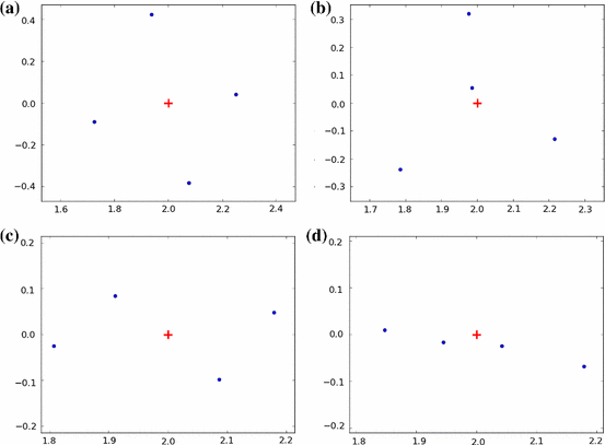

  

  The four first cases of Example 2.12 (the fifth one, less visual, does not appear here): the red cross is $\theta$ and the blue circular dots are the outliers of ${\mathbf {A}}_n+{\mathbf {P}}_n$ tending to $\theta _1$. Each figure is made with the simulation of ${\mathbf {A}}_n$ a renormalized Ginibre matrix with size $2.10^3$ plus ${\mathbf {P}}_n$ (whose choice depends of course of the case) with $\theta =2$. a The blue dots draw a square with center $\approx \theta$ at distance $\approx n^{-1/8}$ from $\theta$. b The blue dots draw an equilateral triangle with center $\approx \theta$ at distance $\approx n^{-1/6}$ from $\theta$ plus a point at distance $\approx n^{-1/2}$ from $\theta$. c The blue dots draw two crossing segments with centers $\approx \theta$ and lengths $\approx n^{-1/4}$. d The blue dots draw a segment with center $\approx \theta$ and length $\approx n^{-1/4}$ plus two points at distance $\approx n^{-1/2}$ from $\theta$

• (b) The JCF of ${\mathbf {P}}_n$ for $\theta$ has one block with size $3$ and one block with size $1$ (so that $\alpha _1=2$, $(p_{1,1},\beta _{1,1})=(3,1)$, $(p_{1,2},\beta _{1,2})=(1,1)$): then the $4$ outliers of $\widetilde{{\mathbf {A}}}_n$ are the vertices of an equilateral triangle with center $\approx \theta$ and size $\approx n^{-1/6}$ plus a point at distance $\approx n^{-1/2}$ from $\theta$ [the three first ones behave like the three third roots of the variable $\theta m_{1,1}^\theta$ and the last one behaves like $\theta (m_{4,4}^{\theta } - m_{1,4}^{\theta }m_{4,1}^{\theta }/m_{1,1}^{\theta })$ where $m_{1,1}^{\theta },m_{1,4}^{\theta },m_{4,1}^\theta ,m_{4,4}^\theta$ are Gaussian variables with correlations given by (7)].

• (c) The JCF of ${\mathbf {P}}_n$ for $\theta$ has two blocks with size $2$ (so that $\alpha _1=1$, $(p_{1,1},\beta _{1,1})=(2,2)$): then the $4$ outliers of $\widetilde{{\mathbf {A}}}_n$ are the extremities of two crossing segments with centers $\approx \theta$ and size $\approx n^{-1/4}$ [their limit distribution is the one of the square roots of the eigenvalues of the matrix

  $$\begin{aligned} M^{\theta }_1 = \theta \begin{pmatrix}m_{1,1}^{\theta } &{} m_{1,3}^{\theta }\\ m_{3,1}^{\theta } &{} m_{3,3}^{\theta } \\ \end{pmatrix}\end{aligned}$$

  where $m_{1,1}^{\theta },m_{1,3}^{\theta },m_{3,1}^\theta ,m_{3,3}^\theta$ are Gaussian variables with correlations given by (7)].

• (d) The JCF of ${\mathbf {P}}_n$ for $\theta$ has one block with size $2$ and two blocks with size $1$ (so that $\alpha _1=2$, $(p_{1,1},\beta _{1,1})=(2,1)$, $(p_{1,2},\beta _{1,2})=(1,2)$ ): then the $4$ outliers of $\widetilde{{\mathbf {A}}}_n$ are the extremities of a segment with center $\approx \theta$ and size $\approx n^{-1/4}$ plus two points at distance $\approx n^{-1/2}$ from $\theta$ [(the two first ones behave like the square roots of $\theta m_{1,1}^\theta$ and the two last ones behave like the eigenvalues of the matrix

  $$\begin{aligned} M_2^\theta = \theta \begin{pmatrix}m_{3,3}^\theta &{} m_{3,4}^\theta \\ m_{4,3}^\theta &{} m_{4,4}^\theta \end{pmatrix}- \frac{\theta }{m_{1,1}^\theta } \begin{pmatrix}m_{3,1}^\theta \\ m_{4,1}^\theta \end{pmatrix}\begin{pmatrix}m_{1,3}^\theta&m_{1,4}^\theta \end{pmatrix}\end{aligned}$$

  where the $m_{i,j}^\theta$’s are Gaussian variables with correlations given by (7)].

• (e) The JCF of ${\mathbf {P}}_n$ for $\theta$ has four blocks with size $1$ [so that $\alpha _1=1$, $(p_{1,1},\beta _{1,1})=(1,4)$]: then the $4$ outliers of $\widetilde{{\mathbf {A}}}_n$ are four points at distance $\approx n^{-1/2}$ from $\theta$ [their limit distribution is the one of the eigenvalues of the matrix

  $$\begin{aligned} M_1^\theta = \theta \begin{pmatrix}m_{1,1}^\theta &{}\quad m_{1,2}^\theta &{}\quad m_{1,3}^\theta &{}\quad m_{1,4}^\theta \\ m_{2,1}^\theta &{}\quad m_{2,2}^\theta &{}\quad m_{2,3}^\theta &{}\quad m_{2,4}^\theta \\ m_{3,1}^\theta &{}\quad m_{3,2}^\theta &{}\quad m_{3,3}^\theta &{}\quad m_{3,4}^\theta \\ m_{4,1}^\theta &{}\quad m_{4,2}^\theta &{}\quad m_{4,3}^\theta &{}\quad m_{4,4}^\theta \\ \end{pmatrix}\end{aligned}$$

  where the $m_{i,j}^\theta$’s are Gaussian variables with correlations given by (7)].

2.3 Examples

2.3.1 Uncorrelated case

Let us suppose that

$$\begin{aligned}&\displaystyle \forall i,i^{\prime }=1, \ldots ,q,\; \forall (k,\ell , k^{\prime }, \ell ^{\prime })\in J(\theta _i)\times I(\theta _i)\times J(\theta _{i^{\prime }})\times I(\theta _{i^{\prime }}),\\&\displaystyle {\mathbf {e}}_{ k}^*{\mathbf {Q}}^{-1}({\mathbf {Q}}^{-1})^*{\mathbf {e}}_{ {k^{\prime }}}\;\cdot \;{\mathbf {e}}_{ \ell ^{\prime }}^*{\mathbf {Q}}^*{\mathbf {Q}}\, {\mathbf {e}}_{ {\ell }}={1\!\!1}_{k=k^{\prime },\, \ell =\ell ^{\prime }}\nonumber \end{aligned}$$

(10)

Note that it is the case when in (7), ${\mathbf {Q}}$ is unitary, i.e. when ${\mathbf {P}}$ is unitarily conjugated to $\begin{pmatrix}{\mathbf {J}}&{}0\\ 0&{}0\end{pmatrix}$, with ${\mathbf {J}}$ as in (4).

By (7), Hypothesis (10) implies that the entries $m_{k,\ell }^{\theta _i}$ of the random vector of (6) are independent and that each $m_{k,\ell }^{\theta _i}$ has a distribution which depends only on $\theta _i$. Let us introduce some notation. For $\beta$ a positive integer, we define³

$$\begin{aligned}&{\text {Ginibre}}(\beta ):=\beta \times \beta \,\text { random matrix with i.i.d. }\,{\fancyscript{N}}_{{\mathbb {C}}}(0,1)\,\text { entries}, \end{aligned}$$

(11)

$$\begin{aligned} \nonumber \\&{\text {Ginibre}}(\beta , \beta ^{\prime }):=\beta \times \beta ^{\prime }\,\text { random matrix with i.i.d. }\,{\fancyscript{N}}_{{\mathbb {C}}}(0,1)\,\text { entries}, \end{aligned}$$

(12)

and we get the following corollary:

Corollary 2.13

If Hypothesis (10) holds, then:

• 1. The collection of random vectors $\displaystyle \left( \Lambda _{i,1},\Lambda _{i,2},\ldots ,\Lambda _{i,\alpha _i} \right)$, indexed by $i=1, \ldots , q$, i.e. by the distinct limit outliers $\theta _i$, is asymptotically independent,

• 2. For each $i=1, \ldots , q$ and each $j=1, \ldots , \alpha _i$, the matrix ${\mathbf {M}}_j^{\theta _i}$ is distributed as:

  • If $j=1$, then

    $$\begin{aligned} {\mathbf {M}}_j^{\theta _i}\sim \frac{\theta _i\, b}{ \sqrt{|\theta _i|^2-b^2}}{\text {Ginibre}}(\beta _{i,j}), \end{aligned}$$

  • If $j>1$, then

    $$\begin{aligned}&{\mathbf {M}}_j^{\theta _i}\sim \frac{\theta _i\, b}{ \sqrt{|\theta _i|^2-b^2}}\left( {\text {Ginibre}}(\beta _{i,j})-{\text {Ginibre}}(\beta _{i,j},\rho _{i,j})\times {\text {Ginibre}}(\rho _{i,j})^{-1}\right. \\&\left. \qquad \times {\text {Ginibre}}(\rho _{i,j},\beta _{i,j})\right) , \end{aligned}$$

  where the four Ginibre matrices involved if $j>1$ are independent and where $\rho _{i,j}=\sum _{j^{\prime }=1}^{j-1}\beta _{i,j^{\prime }}$.

Remark 2.14

• The first part of this corollary means that under Hypothesis (10), the fluctuations of outliers of $\widetilde{{\mathbf {A}}}_n$ with different limits are independent. We will see below that it is not always true anymore if Hypothesis (10) does not hold.

• In the second part of this corollary, $j=1$ means that $p_{i,j}=\max _{j^{\prime }} p_{i,j^{\prime }}$, i.e. that we consider the outliers of $\widetilde{{\mathbf {A}}}_n$ at the largest possible distance ($\approx n^{-1/(2p_{i,1})}$) from $\theta _i$.

• In the second part of the corollary, for $j>1$, the four matrices involved are independent, but the ${\mathbf {M}}_j^{\theta _i}$’s are not independent as $j$ varies (the reason is that the matrix $M_j^{\theta _i,{\mathrm {I}}}$ of (9) contains $M_{j^{\prime }}^{\theta _i,{\mathrm {I}}{\mathrm {V}}}$ as a submatrix as soon as $j^{\prime }<j$).

• If one weakens Hypothesis (10) by supposing it to hold only for $i=i^{\prime }$ (resp. $i\ne i^{\prime }$), then only the second (resp. first) part of the corollary stays true.

The $i=i^{\prime }$ case of the last point of the previous remark implies the following corollary.

Corollary 2.15

If, for a certain $i$, $\alpha _i=\beta _{i,1}=1$ (i.e. if $\theta _i$ is an eigenvalue of ${\mathbf {P}}$ with multiplicity⁴ $p_{i,1}$ but with associated eigenspace having dimension one), then the random vector

$$\begin{aligned} \displaystyle \left( n^{1/(2p_{i,1})} \cdot \left( {}^{\;\;\theta _i}_{p_{i,1}}\widetilde{\lambda }_{s,1} - \theta _i \right) \right) _{1\le s\le p_{i,1}} \end{aligned}$$

converges in distribution to the vector of the ${p_{i,1}}^{\text {th}}$ roots of a ${\fancyscript{N}}_{{\mathbb {C}}}(0, \frac{b^2}{|\theta _i|^2(|\theta _i|^2-b^2)})$ random variable.

2.3.2 Correlated case

If Hypothesis (10) does not hold anymore, then the individual and joint distributions of the random matrices ${\mathbf {M}}^{\theta _i}_j$ are not anymore related to Ginibre matrices as in Corollary 2.13: the entries of the matrices $M_j^{\theta _i,{\mathrm {I}},{\mathrm {I}}{\mathrm {I}},{\mathrm {I}}{\mathrm {I}}{\mathrm {I}},{\mathrm {I}}{\mathrm {V}}}$ of (9) can have non uniform variances, even be correlated, and one can also have correlations between the entries of two matrices ${\mathbf {M}}^{\theta _i}_j$, ${\mathbf {M}}^{\theta _{i^{\prime }}}_{j^{\prime }}$ for $\theta _i\ne \theta _{i^{\prime }}$. This last case has the surprising consequence that outliers of $\widetilde{{\mathbf {A}}}_n$ with different limits can be asymptotically correlated. Such a situation had so far only been brought to light, by Knowles and Yin [25], for deformation of non Gaussian Wigner matrices. Note that in our model no restriction on the distributions of the deformed matrix ${\mathbf {A}}_n$ is made (${\mathbf {A}}_n$ can for example be a renormalized Ginibre matrix). The following corollary gives an example of a simple situation where such correlations occur. This simple situation corresponds to the following case: we suppose that for some $i\ne i^{\prime }$ in $\{1, \ldots , q\}$, we have $\beta _{i,1}=\beta _{i^{\prime },1}=1$. We let $\ell$ and $\ell ^{\prime }$ (resp. $k$ and $k^{\prime }$) denote the indices in $\{1, \ldots , r\}$ corresponding to the last (resp. first) columns of the block ${\mathbf {R}}_{p_{i,1}}(\theta _i)$ and of the block ${\mathbf {R}}_{p_{i^{\prime },1}}(\theta _{i^{\prime }})$ and set

$$\begin{aligned} K:={\mathbf {e}}_{ k}^*{\mathbf {Q}}^{-1}\left( {\mathbf {Q}}^{-1}\right) ^*{\mathbf {e}}_{ {k^{\prime }}}\;\cdot \;{\mathbf {e}}_{ \ell ^{\prime }}^*{\mathbf {Q}}^*{\mathbf {Q}}\, {\mathbf {e}}_{ {\ell }}. \end{aligned}$$

(13)

We will see in the next corollary that as soon as $K\ne 0$, the fluctuations of outliers at macroscopic distance from each other (i.e. with distinct limits) are not independent. Set

$$\begin{aligned} \sigma ^2&:= \frac{|\theta _i|^2b^2}{|\theta _i|^2-b^2}{\mathbf {e}}_{ k}^*{\mathbf {Q}}^{-1}\left( {\mathbf {Q}}^{-1}\right) ^*{\mathbf {e}}_{ {k}}\;\cdot \;{\mathbf {e}}_{ \ell }^*{\mathbf {Q}}^*{\mathbf {Q}}\, {\mathbf {e}}_{ {\ell }}\; ,\nonumber \\ {\sigma ^{\prime }}^2&:= \frac{|\theta _{i^{\prime }}|^2b^2}{|\theta _{i^{\prime }}|^2-b^2}{\mathbf {e}}_{ k^{\prime }}^*{\mathbf {Q}}^{-1}\left( {\mathbf {Q}}^{-1}\right) ^*{\mathbf {e}}_{ {k^{\prime }}}\;\cdot \;{\mathbf {e}}_{ \ell ^{\prime }}^*{\mathbf {Q}}^*{\mathbf {Q}}\, {\mathbf {e}}_{ {\ell ^{\prime }}}. \end{aligned}$$

(14)

Corollary 2.16

Under this hypothesis, for any $1\le s\le p_{i,1}$ and any $1\le s^{\prime }\le p_{i^{\prime },1}$, as $n\rightarrow \infty$, the random vector

$$\begin{aligned} (Z_n, Z_n^{\prime }):=\left( \sqrt{n}\left( {}^{\;\;\theta _i}_{p_{i,1}}\widetilde{\lambda }_{s,1} - \theta _i \right) ^{p_{i,1}} , \;\sqrt{n} \left( {{}^{\;\;\theta _{i'}}_{p_{i^{\prime },1}}\widetilde{\lambda }_{s^{\prime },1} - \theta _{i^{\prime }} }\right) ^{p_{i^{\prime },1}}\right) \end{aligned}$$

(15)

converges in distribution to a complex centered Gaussian vector $(Z,Z^{\prime })$ defined by

$$\begin{aligned} Z\sim {\fancyscript{N}}_{{\mathbb {C}}}(0, \sigma ^2)\,,\quad Z^{\prime }\sim {\fancyscript{N}}_{{\mathbb {C}}}(0, {\sigma ^{\prime }}^2) \,,\quad {\mathbb {E}}[ZZ^{\prime }]=0\,,\quad {\mathbb {E}}[Z\overline{Z^{\prime }}]=\frac{\theta _i\overline{\theta _{i^{\prime }}}\, b^2 \,K}{\theta _i\overline{\theta _{i^{\prime }}}-b^2}. \end{aligned}$$

(16)

Example 2.17

Let us illustrate this corollary (which is already an example) by a still more particular example. Suppose that ${\mathbf {A}}_n$ is a renormalized Ginibre matrix and that for $\theta =1.5+i$, $\theta ^{\prime }=3+i$ and for $\kappa \in {\mathbb {R}}\backslash \{-1,1\}$, ${\mathbf {Po}}$ is given by

$$\begin{aligned} {\mathbf {Po}}={\mathbf {Q}}\begin{pmatrix}\theta &{}0\\ 0&{}\theta ^{\prime }\end{pmatrix}{\mathbf {Q}}^{-1}\; ,\qquad \qquad {\mathbf {Q}}=\begin{pmatrix}1&{}\kappa \\ \kappa &{}1\end{pmatrix}\,. \end{aligned}$$

In this case, $q=2$, $\alpha _1=\alpha _2=p_{1,1}=p_{2,1}=\beta _{1,1}=\beta _{2,1}=1$ and $\ell =k=1$, $\ell ^{\prime }=k^{\prime }=2$. Thus ${\mathbf {A}}_n+{\mathbf {P}}_n$ has two outliers $\widetilde{\lambda }_n:={}^{\;\;\theta }_{p_{1,1}}\widetilde{\lambda }_{1,1}$ and $\widetilde{\lambda ^{\prime }}_n:={}^{\;\;\theta ^{\prime }}_{p_{2,1}}\widetilde{\lambda }_{1,1}$ and one can compute the numbers $K, \sigma , \sigma ^{\prime }$ of (13), (14) and get

$$\begin{aligned} \sigma ^2&=\frac{\left( 1+\kappa ^2\right) ^2}{\left( 1-|\theta |^{-2}\right) \left( 1-\kappa ^2\right) ^2}\nonumber \\ {\sigma ^{\prime }}^2&=\frac{\left( 1+\kappa ^2\right) ^2}{\left( 1-|\theta ^{\prime }|^{-2}\right) \left( 1-\kappa ^2\right) ^2}\quad {\mathbb {E}}\left[ Z\overline{Z^{\prime }}\right] =\frac{-4\kappa ^2}{\left( 1-(\theta \overline{\theta ^{\prime }})^{-1}\right) \left( 1-\kappa ^2\right) ^2}. \end{aligned}$$

(17)

We see that for $\kappa =0$, $Z_n=\sqrt{n}(\widetilde{\lambda } -\theta )$ and $Z_n^{\prime }=\sqrt{n}(\widetilde{\lambda ^{\prime }} -\theta ^{\prime })$ are asymptotically independent, but that for $\kappa \ne 0$, $Z_n$ and $Z_n^{\prime }$ are not asymptotically independent anymore. This phenomenon and the accuracy of the approximation $(Z_n,Z_n^{\prime })\approx (Z,Z^{\prime })$ for $n\gg 1$ are illustrated by Table 1 and Fig. 4, where $10^3$ samples of $(Z_n,Z_n^{\prime })$ have been simulated for $n=10^3$.

Table 1 Comparison between theoretical asymptotic formulas (16) and (17) and a Monte-Carlo numerical computation made out of $10^3$ matrices with size $n=10^3$

Fig. 4

Lack of correlation/correlation between outliers with different limits: abscissas (resp. ordinates) of the dots are $X:=\mathfrak {I}(Z_n)$ (resp. $Y:=\mathfrak {I}(Z_n^{\prime })$) for $10^3$ independent copies of $(Z_n,Z_n^{\prime })$ (computed thanks to matrices with size $n=10^3$ as for Table 1). a $\kappa =0$: uncorrelated case. b $\kappa =2^{-1/2}$: correlated case. The straight line is the theoretical optimal regression line (i.e. the line with equation $y=ax$ where $a$ minimizes the variance of $Y-aX$, computed thanks to the asymptotic formulas (16) and (17)): one can notice that it fits well with the empirical datas

2.4 Preliminaries to the proofs

First, for notational brevity, from now on, $n$ will be an implicit parameter (${\mathbf {A}}:={\mathbf {A}}_n$, ${\mathbf {P}}:={\mathbf {P}}_n$, ...), except in case of ambiguity.

Secondly, from now on, we shall suppose that ${\mathbf {T}}$ is deterministic. Indeed, once the results established with ${\mathbf {T}}$ deterministic, as ${\mathbf {T}}$ is independent from the others random variables and the only relevant parameter $b$ is deterministic, we can condition on ${\mathbf {T}}$ and apply the deterministic result. So we suppose that ${\mathbf {T}}$ is deterministic and that there is a constant $M$ independent of $n$ such that for all $n$,

$$\begin{aligned} \Vert {\mathbf {T}}\Vert _{{{\mathrm{op}}}} \le M. \end{aligned}$$

Thirdly, as the set of probability measures supported by $[0, M]$ is compact, up to an extraction, one can suppose that there is a probability measure $\Theta$ on $[0,M]$ such that the ESD of ${\mathbf {T}}$ converges to $\Theta$ as $n\rightarrow \infty$. We will work within this subsequence. This could seem to give a partial convergence result, but in fact, what is proved is that from any subsequence, one can extract a subsequence which converges to the limit given by the theorem. This is of course enough for the proof. Note that by Hypothesis 1, we have $b^2=\int x^2 \Theta (dx)$. Having supposed that the ESD of ${\mathbf {T}}$ converges to $\Theta$ insures that ${\mathbf {A}}$ satisfies the hypotheses⁵ of the Single Ring Theorem of [18] and of the paper [19]. We will use it once, in the proof of Lemma 6.1, where we need one of the preliminary results of [19].

At last, notice that ${\mathbf {A}}+{\mathbf {P}}$ and ${\mathbf {V}}({\mathbf {A}}+{\mathbf {P}}) {\mathbf {V}}^*$ have the same spectrum, that

$$\begin{aligned} \ {\mathbf {V}}({\mathbf {A}}+ {\mathbf {P}}) {\mathbf {V}}^* = {\mathbf {V}}{\mathbf {U}}{\mathbf {T}}+ {\mathbf {V}}{\mathbf {P}}{\mathbf {V}}^*, \end{aligned}$$

(18)

and that as ${\mathbf {U}}$ and ${\mathbf {V}}$ are independent Haar-distributed matrices, ${\mathbf {V}}{\mathbf {U}}$ and ${\mathbf {V}}$ are also Haar-distributed and independent. It follows that we shall, instead of the hypotheses made above the statement of Hypotheses 1, 2, and 3, suppose that:

$$\begin{aligned}&{\mathbf {A}}= {\mathbf {U}}{\mathbf {T}}\quad \text {with}\quad {\mathbf {T}}\text { deterministic and } {\mathbf {U}}\text { Haar-distributed}\nonumber \\&\text { and }\quad {\mathbf {P}}\text { is independent of }{\mathbf {A}}\text { and invariant, in law,}\nonumber \\&\quad \text { by conjugation by any unitary matrix.} \end{aligned}$$

(19)

In the sequel ${\mathbb {E}}_{\mathbf {U}}$ will denote the expectation with respect to the randomness of ${\mathbf {U}}$ and not to the one of ${\mathbf {P}}$. In the same way, ${\mathbb {E}}_{\mathbf {P}}$ will denote the expectation with respect to the randomness of ${\mathbf {P}}$.

2.5 Sketch of the proofs

We start with the following trick, now quite standard in spiked models. Let ${\mathbf {B}}\in {\fancyscript{M}}_{n\times r}({\mathbb {C}})$ and ${\mathbf {C}}\in {\fancyscript{M}}_{r\times n}({\mathbb {C}})$ such that ${\mathbf {P}}= {\mathbf {B}}{\mathbf {C}}$ (where ${\fancyscript{M}}_{p\times q}({\mathbb {C}})$ denotes the rectangular complex matrices of size $p\times q$). Then

$$\begin{aligned} \det \left( z{\mathbf {I}}- \widetilde{{\mathbf {A}}}\right)= & {} \det (z{\mathbf {I}}- ({\mathbf {A}}+ {\mathbf {P}})) \nonumber \\= & {} \det (z{\mathbf {I}}- {\mathbf {A}}) \det \left( {\mathbf {I}}- (z{\mathbf {I}}- {\mathbf {A}})^{-1}{\mathbf {P}}\right) \nonumber \\= & {} \det (z{\mathbf {I}}- {\mathbf {A}}) \det \left( {\mathbf {I}}- (z{\mathbf {I}}- {\mathbf {A}})^{-1}{\mathbf {B}}{\mathbf {C}}\right) \nonumber \\= & {} \det (z{\mathbf {I}}- {\mathbf {A}}) \det \left( {\mathbf {I}}- {\mathbf {C}}(z{\mathbf {I}}- {\mathbf {A}})^{-1}{\mathbf {B}}\right) . \end{aligned}$$

(20)

For the last step, we used the fact that for all ${\mathbf {M}}\in {\fancyscript{M}}_{r\times n}$ and ${\mathbf {N}}\in {\fancyscript{M}}_{n\times r}({\mathbb {C}})$, $\det \left( {\mathbf {I}}_r + {\mathbf {M}}{\mathbf {N}}\right) = \det \left( {\mathbf {I}}_n + {\mathbf {N}}{\mathbf {M}}\right)$. Therefore, the eigenvalues $z$ of $\widetilde{{\mathbf {A}}}$ which are not eigenvalues of ${\mathbf {A}}$ are characterized by

$$\begin{aligned} \det \left( {\mathbf {I}}- {\mathbf {C}}(z{\mathbf {I}}- {\mathbf {A}})^{-1}{\mathbf {B}}\right) = 0. \end{aligned}$$

(21)

In view of (20), as previously done by Tao in [30], we introduce the meromorphic functions (implicitly depending on $n$)

$$\begin{aligned} f(z):= & {} \det \left( {\mathbf {I}}- {\mathbf {C}}(z{\mathbf {I}}- {\mathbf {A}})^{-1}{\mathbf {B}}\right) = \ \frac{\det \left( z{\mathbf {I}}- \widetilde{{\mathbf {A}}}\right) }{\det (z{\mathbf {I}}- {\mathbf {A}})}, \end{aligned}$$

(22)

$$\begin{aligned} g(z):= & {} \det \left( {\mathbf {I}}- {\mathbf {C}}(z{\mathbf {I}})^{-1} {\mathbf {B}}\right) = \frac{\det (z{\mathbf {I}}- {\mathbf {P}})}{\det (z{\mathbf {I}})} \end{aligned}$$

(23)

and aim to study the zeros of $f$.

• The proof of Theorem 2.5 (eigenvalues outside the outer circle) relies on the fact that on the domain $\{|z|>b+2\varepsilon \}$, $f(z)\approx g(z)$. This follows from the fact that for $|z|>b+2\varepsilon$, the $n\times n$ matrix $(z{\mathbf {I}}-{\mathbf {A}})^{-1}-z^{-1}{\mathbf {I}}$ has small entries, and even satisfies

  $$\begin{aligned} {\mathbf {x}}^*\left( (z{\mathbf {I}}-{\mathbf {A}})^{-1}-z^{-1}{\mathbf {I}}\right) {\mathbf {y}}\ll 1 \end{aligned}$$

  (24)

  for deterministic unitary column vectors ${\mathbf {x}}, \mathbf {y}$.

• The proof of Theorem 2.6 (lack of eigenvalues inside the inner circle) relies on the fact that for $|z|<a-\delta$, $\left\| {\mathbf {C}}(z{\mathbf {I}}- {\mathbf {A}})^{-1}{\mathbf {B}}\right\| _{{{\mathrm{op}}}} < 1$. We will see that it follows from estimates as the one of (24) for ${\mathbf {A}}$ replaced by ${\mathbf {A}}^{-1}$.

• The most difficult part of the article is the proof of Theorem 2.10 about the fluctuations of the outliers around their limits $\theta _i$ ($1\le i\le q$). As the outliers are the zeros of $f$, we shall expand $f$ around any fixed $\theta _i$. Specifically, for each block size $p_{i,j}$ ($1\le j\le \alpha _i$), we prove at Lemma 5.1 that for $\pi _{i,j} :=\sum _{l > j} \beta _{{i,l}}p_{i,l}$ and ${\mathbf {M}}^{\theta _i}_j$ the matrix with size⁶ $\beta _{i,j}$ defined above, we have

  $$\begin{aligned} f\left( \theta _i + \frac{z}{n^{1/(2p_{i,j})}} \right) \ \approx \ z^{\pi _{i,j}} \cdot \det \left( z^{p_{i,j}}-{\mathbf {M}}^{\theta _i}_j\right) . \end{aligned}$$

  (25)

  This proves that ${\mathbf {A}}+{\mathbf {P}}$ has $\pi _{i,j}$ outliers tending to $\theta _i$ at rate $\ll n^{-1/(2p_{i,j})}$, has $p_{i,j}\times \beta _{i,j}$ outliers tending to $\theta _i$ at rate $n^{-1/(2p_{i,j})}$ and that these $p_{i,j}\times \beta _{i,j}$ outliers are distributed as the ${p_{i,j}}^{\text {th}}$ roots of the eigenvalues of ${\mathbf {M}}^{\theta _i}_{j}$. We see that the key result in this proof is the estimate (25). To prove it, we first specify the choice of the already introduced matrices ${\mathbf {B}}\in {\fancyscript{M}}_{n\times r}({\mathbb {C}})$ and ${\mathbf {C}}\in {\fancyscript{M}}_{r\times n}({\mathbb {C}})$ such that ${\mathbf {P}}= {\mathbf {B}}{\mathbf {C}}$ by imposing moreover that ${\mathbf {C}}{\mathbf {B}}={\mathbf {J}}$ (recall that ${\mathbf {J}}$ is the $r\times r$ Jordan Canonical Form of ${\mathbf {P}}$ of (4)). Then, for

  $$\begin{aligned} \tilde{z}:=\theta _i + \frac{z}{n^{1/(2p_{i,j})}}\, ,\qquad {\mathbf {X}}_n^{\tilde{z}}:=\sqrt{n}{\mathbf {C}}\left( (\tilde{z}{\mathbf {I}}-{\mathbf {A}})^{-1}-\tilde{z}^{-1}{\mathbf {I}}\right) {\mathbf {B}}\, , \end{aligned}$$

  we write

  $$\begin{aligned} \nonumber f\left( \tilde{z} \right)= & {} \det \left( {\mathbf {I}}- \frac{1}{\tilde{z}} {\mathbf {J}}- \frac{1}{\sqrt{n}} {\mathbf {X}}_n^{\tilde{z}} \right) \\ \nonumber= & {} \det \left( {\mathbf {I}}- \theta _i^{-1}{\mathbf {J}}+ \theta _i^{-1}\left( 1 - \frac{1}{1+n^{-1/(2p_{i,j})} z \theta _i^{-1}} \right) {\mathbf {J}}- \frac{1}{\sqrt{n}} {\mathbf {X}}_n^{\tilde{z}} \right) \\\approx & {} \det \left( {\mathbf {I}}- \theta _i^{-1}{\mathbf {J}}+ \frac{z \theta _i^{-2}}{n^{1/(2p_{i,j})}}{\mathbf {J}}- \frac{1}{\sqrt{n}} {\mathbf {X}}_n^{\tilde{z}} \right) \end{aligned}$$

  (26)

  At this point, one has to note that (obviously) $\det \left( {\mathbf {I}}- \theta _i^{-1}{\mathbf {J}}\right) = 0$ and that (really not obviously) the $r\times r$ random array ${\mathbf {X}}_n^{\tilde{z}}$ converges in distribution to a Gaussian array as $n\rightarrow \infty$ (this is proved thanks to the Weingarten calculus). Then the result will follow from a Taylor expansion of (26) and a careful look at the main contributions to the determinant.

3 Eigenvalues outside the outer circle: proof of Theorem 2.5

We start with Eqs. (20) and (21), established in the previous Section, and the functions $f$ and $g$, introduced at (22) and (23).

Lemma 3.1

As $n$ goes to infinity, we have

$$\begin{aligned} \sup _{|z| \ge b + 2\varepsilon } \left| f(z) - g(z) \right| \ \overset{({\mathbb {P}})}{\longrightarrow }\ 0. \end{aligned}$$

Before proving the lemma, let us explain how it allows to conclude the proof of Theorem 2.5. The poles of $f$ and $g$ are respectively eigenvalues of the ${\mathbf {A}}$ and of the null matrix, hence for $n$ large enough, they have no pole in the region $\left\{ z \in {\mathbb {C}}\; ;\;|z| > b+ 2\varepsilon \right\}$, whereas their zeros in this region are precisely the eigenvalues of respectively $\widetilde{{\mathbf {A}}}$ and ${\mathbf {P}}$ that are in this region. But $|g|$ admits the following lower bound on the circle with radius $b+\varepsilon$: as we assumed that any eigenvalue of ${\mathbf {P}}$ is at least at distance at least $\varepsilon$ from $\left\{ z \in {\mathbb {C}}\; ;\;\ |z| = b + 2\varepsilon \right\}$, one has

$$\begin{aligned} \inf _{|z| = b + 2 \varepsilon }|g(z)| = \inf _{|z| = b + 2 \varepsilon } \frac{\prod _{i=1}^n \left| z - \lambda _i({\mathbf {P}}) \right| }{|z|^n}\ge & {} \left( \frac{\varepsilon }{b + 2 \varepsilon }\right) ^r , \end{aligned}$$

so that by the previous lemma, with probability tending to one,

$$\begin{aligned} \forall z\in {\mathbb {C}}, |z|=b+2\varepsilon \implies |f(z)-g(z)|<|g(z)|, \end{aligned}$$

and so, by Rouché’s Theorem [5], p. 131], we know that inside the region $\left\{ z \in {\mathbb {C}}, |z| \le b+ 2\varepsilon \right\}$, $f$ and $g$ have the same number of zeros (since they both have $n$ poles). Therefore, as their total number of zeros is $n$, $f$ and $g$ have the same number of zeros outside this region.

Also, Lemma 3.1 allows to conclude that, after a proper labeling

$$\begin{aligned} \forall i \in \{1,\ldots ,r_b \}, \ \ \lambda _i(\widetilde{{\mathbf {A}}}) - \lambda _i({\mathbf {P}}) \ \overset{({\mathbb {P}})}{\longrightarrow }\ 0. \end{aligned}$$

Indeed, for each fixed $i\in \{1, \ldots , r_b\}$,

$$\begin{aligned} \prod _{j=1}^{r} \left| 1 - \frac{\lambda _j({\mathbf {P}})}{\lambda _i(\widetilde{{\mathbf {A}}})}\right| = \left| g(\lambda _i(\widetilde{{\mathbf {A}}})) \right|= & {} \left| f(\lambda _i(\widetilde{{\mathbf {A}}})) - g(\lambda _i(\widetilde{{\mathbf {A}}}))\right| \\\le & {} \sup _{|z| \ge b + 2\varepsilon } \left| f(z) - g(z) \right| \ \overset{({\mathbb {P}})}{\longrightarrow }\ 0. \end{aligned}$$

Let us now explain how to prove Lemma 3.1. One can notice at first that it suffices to prove that

$$\begin{aligned} \sup _{|z| \ge b + 2\varepsilon } \left\| {\mathbf {C}}(z{\mathbf {I}}- {\mathbf {A}})^{-1}{\mathbf {B}}- {\mathbf {C}}(z{\mathbf {I}})^{-1}{\mathbf {B}}\right\| _{{{\mathrm{op}}}} \ \overset{({\mathbb {P}})}{\longrightarrow }\ 0, \end{aligned}$$

(27)

simply because the function $\det : {\fancyscript{M}}_r({\mathbb {C}}) \rightarrow {\mathbb {C}}$ is Lipschitz over every bounded set of ${\fancyscript{M}}_r({\mathbb {C}})$. Then, the proof of Lemma 3.1 is based on both following lemmas (whose proofs are postponed to Sect. 6).

Lemma 3.2

There exists a constant $C_1>0$ such that the event

$$\begin{aligned} {\fancyscript{E}}_n:=\left\{ \forall k \ge 1, \ \ \left\| {\mathbf {A}}^k\right\| _{{{\mathrm{op}}}} \ \le \ C_1 \cdot (b+ \varepsilon )^k\right\} \end{aligned}$$

has probability tending to one as $n$ tends to infinity.

Lemma 3.3

For all $k \ge 0$, as $n$ goes to infinity, we have

$$\begin{aligned} \left\| {\mathbf {C}}{\mathbf {A}}^k {\mathbf {B}}\right\| _{{{\mathrm{op}}}} \ \overset{({\mathbb {P}})}{\longrightarrow }\ 0. \end{aligned}$$

On the event ${\fancyscript{E}}_n$ defined at Lemma 3.2 above, we write, for $|z| \ge b + 2\varepsilon$,

$$\begin{aligned} {\mathbf {C}}(z{\mathbf {I}}- {\mathbf {A}})^{-1}{\mathbf {B}}- {\mathbf {C}}(z{\mathbf {I}})^{-1}{\mathbf {B}}= & {} {\mathbf {C}}\sum _{k=1}^{+\infty } \frac{{\mathbf {A}}^k}{z^{k+1}} {\mathbf {B}}. \end{aligned}$$

and it suffices to write that for any $\delta >0$,

$$\begin{aligned}&{\mathbb {P}}\left( \sup _{|z|\ge b+2\varepsilon } \left\| {\mathbf {C}}(z{\mathbf {I}}- {\mathbf {A}})^{-1}{\mathbf {B}}- {\mathbf {C}}(z{\mathbf {I}})^{-1}{\mathbf {B}}\right\| _{{{\mathrm{op}}}} > \delta \right) \\&\quad \le {\mathbb {P}}\left( {\fancyscript{E}}_n^c\right) + {\mathbb {P}}\left( \sum _{k=1}^{k_0} \frac{\left\| {\mathbf {C}}{\mathbf {A}}^k{\mathbf {B}}\right\| _{{{\mathrm{op}}}}}{(b+2\varepsilon )^{k+1}} > \frac{\delta }{2}\right) \\&\qquad +{\mathbb {P}}\left( {\fancyscript{E}}_n\text { and }\left\| {\mathbf {C}}\sum _{k=k_0+1}^{+\infty } \frac{{\mathbf {A}}^k}{(b+2\varepsilon )^{k+1}} {\mathbf {B}}\right\| _{{{\mathrm{op}}}} > \frac{\delta }{2} \right) .\\ \end{aligned}$$

By to Lemma 3.2 and the fact that ${\mathbf {C}}$ and ${\mathbf {B}}$ are uniformly bounded (see Remark 5.2), we can find $k_0$ so that the last event has a vanishing probability. Then, by Lemma 3.3, the probability of the last-but-one event goes to zero as $n$ tends to infinity. This gives (27) and then Lemma 3.1.

4 Lack of eigenvalues inside the inner circle: proof of Theorem 2.6

Our goal here is to show that for all $\delta \in ]0,a[$, with probability tending to one, the function $f$ defined at (22) has no zero in the region $\left\{ z \in {\mathbb {C}}, |z| < a - \delta \right\}$. Recall that

$$\begin{aligned} f(z)= & {} \det \left( {\mathbf {I}}- {\mathbf {C}}(z{\mathbf {I}}- {\mathbf {A}})^{-1}{\mathbf {B}}\right) , \end{aligned}$$

so that a simple sufficient condition would be $\left\| {\mathbf {C}}(z{\mathbf {I}}\!-\! {\mathbf {A}})^{-1}{\mathbf {B}}\right\| _{{{\mathrm{op}}}} {<} 1$ for all $|z| \!<\! a \!-\! \delta$. Thus, it suffices to prove that with probability tending to one as $n$ tends to infinity,

$$\begin{aligned} \sup _{|z| < a - \delta } \left\| {\mathbf {C}}(z{\mathbf {I}}- {\mathbf {A}})^{-1}{\mathbf {B}}\right\| _{{{\mathrm{op}}}} < 1. \end{aligned}$$

By Remark 2.3, we know that ${\mathbf {A}}$ is invertible. As in Sect. 3, we write, for all $|z| < a-\delta$,

$$\begin{aligned} {\mathbf {C}}\left( z{\mathbf {I}}- {\mathbf {A}}\right) ^{-1}{\mathbf {B}}= & {} -{\mathbf {C}}{\mathbf {A}}^{-1} \left( {\mathbf {I}}- z {\mathbf {A}}^{-1} \right) ^{-1}{\mathbf {B}}\\= & {} - {\mathbf {C}}\sum _{k=1}^{\infty } z^{k-1} {\mathbf {A}}^{-k} {\mathbf {B}}. \\ \end{aligned}$$

The idea is to see ${\mathbf {A}}^{-1}$ as an isotropic random matrix such as ${\mathbf {A}}$, since ${\mathbf {A}}^{-1} = {\mathbf {V}}^* {{\mathrm{{diag}}}}(\frac{1}{s_1},\ldots , \frac{1}{s_n}) {\mathbf {U}}^*$, and satisfies the same kind of hypothesis. Indeed, Hypotheses 1 and 2 are automatiquelly satisfied because $a>0$ (see Remark 2.3), and the following lemma, proved in Sect. 6.2, insures us that Hypotheses 3 is also satisfied.

Lemma 4.1

There exist a constant $\widetilde{\kappa } >0$ such that

$$\begin{aligned} {\mathfrak {I}}(z) \ > \ n^{-\widetilde{\kappa }}\Rightarrow & {} \left| {\mathfrak {I}}\left( G_{\mu _{{\mathbf {T}}^{-1}}}(z)\right) \right| \ \le \ \frac{1}{\widetilde{\kappa }}. \end{aligned}$$

Thus, according to [19], the support of $\mu _{{\mathbf {A}}^{-1}}$ converges in probability to the annulus $\left\{ z \in {\mathbb {C}}, \ b^{-1} \le |z| \le a^{-1} \right\}$ as $n\rightarrow \infty$, and so, according to (27),

$$\begin{aligned} \sup _{|\xi | > a^{-1} + \varepsilon } {\mathbf {C}}\sum _{k=1}^{\infty } \frac{{\mathbf {A}}^{-k}}{\xi ^{k+1}} {\mathbf {B}}\ \overset{({\mathbb {P}})}{\longrightarrow }\ 0. \end{aligned}$$

Therefore

$$\begin{aligned}&{\mathbb {P}}\left( \sup _{|z| < a - \delta } \left\| {\mathbf {C}}(zI - {\mathbf {A}})^{-1}{\mathbf {B}}\right\| _{{{\mathrm{op}}}} < 1 \right) \\&\quad \ge \ 1 - {\mathbb {P}}\left( \sup _{|\xi | > a^{-1} + \varepsilon } \left\| {\mathbf {C}}\sum _{k=1}^{\infty } \frac{{\mathbf {A}}^{-k}}{\xi ^{k-1}} {\mathbf {B}}\right\| _{{{\mathrm{op}}}}> 1\right) \ \longrightarrow \ 1 , \end{aligned}$$

with a proper choice for $\varepsilon$. $\square$

5 Proof of Theorem 2.10

5.1 Lemma 5.1 granted proof of Theorem 2.10

Recall that we write ${\mathbf {P}}= {\mathbf {B}}{\mathbf {C}}$ and we know that

$$\begin{aligned} \sup _{|z|>b+2\varepsilon } \left\| {\mathbf {C}}\left( z{\mathbf {I}}-{\mathbf {A}}\right) ^{-1}{\mathbf {B}}- z^{-1}{\mathbf {C}}{\mathbf {B}}\right\| _{{{\mathrm{op}}}} \ \overset{({\mathbb {P}})}{\longrightarrow }\ 0, \end{aligned}$$

(28)

(again, for notational brevity, $n$ will be an implicit parameter, except in case of ambiguity).

Following the ideas of [7], we shall need to differentiate the function $f$ defined at (22) to understand the fluctuations of $\widetilde{\lambda } - \theta$, and to do so, we shall need to be more accurate in the convergence in (28).

Let us first state our key lemma, whose proof is postponed in Sect. 5.3. Recall from (4) that we supposed the JCF of ${\mathbf {P}}$ to have, for the eigenvalue $\theta _i$, $\beta _{{i,1}}$ blocks with size $p_{i,1}$, ......, $\beta _{{i,\alpha _i}}$ blocks with size $p_{i,\alpha _i}$. Recall also that

$$\begin{aligned} f(z)= & {} \det \left( {\mathbf {I}}- {\mathbf {C}}(z{\mathbf {I}}- {\mathbf {A}})^{-1}{\mathbf {B}}\right) . \end{aligned}$$

Lemma 5.1

For all $j \in \{1,\ldots ,\alpha _i\}$, let $F^{\theta _i}_{j}(z)$ be the rational function defined by

$$\begin{aligned} F^{\theta _i}_{j}(z) \ := \ f\left( \theta _i + \frac{z}{n^{1/(2p_{i,j})}} \right) . \end{aligned}$$

(29)

Then, there exists a collection of positive constants $(\gamma _{i,j})_{\displaystyle ^{1\le i\le q}_{1\le j\le \alpha _i}}$ and a collection of non vanishing random variables $(C_{i,j})_{\displaystyle ^{1\le i\le q}_{1\le j\le \alpha _i}}$ independent of $z$, such that we have the convergence in distribution (for the topology of the uniform convergence over any compact set)

$$\begin{aligned} \left( n^{\gamma _{i,j}} F^{\theta _i}_{j}(\cdot ) \right) _{\displaystyle ^{1\le i\le q}_{1\le j\le \alpha _i}}\ \underset{n\rightarrow \infty }{\longrightarrow }\ \left( z\in {\mathbb {C}}\ \mapsto \ z^{\pi _{i,j}}\cdot C_{i,j} \cdot \det \left( z^{p_{i,j}}-{\mathbf {M}}^{\theta _i}_j\right) \right) _{\displaystyle ^{1\le i\le q}_{1\le j\le \alpha _i}} \end{aligned}$$

where ${\mathbf {M}}^{\theta _i}_j$ is the random matrix introduced at (7) and $\pi _{i,j} :=\sum _{l > j} \beta _{{i,l}}p_{i,l}$.

To end the proof of Theorem 2.10, we make sure that we have the right number of eigenvalues of $\widetilde{{\mathbf {A}}}$ thanks to complex analysis considerations (Cauchy formula):

• Eigenvalues tending to $\theta _i$ with the highest convergence rate:

• Lemma 5.1 tells us that on any compact set, $F^{\theta _i}_{j}$ and $z^{\pi _{i,j}}\det (z^{p_{{i,j}}}-{\mathbf {M}}^{\theta _i}_j)$ have the exact same number of roots (for any large enough $n$, the poles of $F^{\theta _i}_{{j}}$ leave any compact set), so, for the smallest block size $p_{i,\alpha _i}$, we know that $F^{\theta _i}_{{\alpha _i}}$ has exactly $\beta _{{i,\alpha _i}} \times p_{i,\alpha _i}$ roots which do not eventually leave any compact set as $n$ goes to infinity.

• Moreover, we know that the only roots of $F_{\alpha _j}^{\theta _i}$ are the $n^{1/(2p_{i,\alpha _i})}(\widetilde{\lambda }-\theta _i)$’s where $\widetilde{\lambda }$ are the eigenvalues of $\widetilde{{\mathbf {A}}}$.

• We conclude that there are exactly $\beta _{{i,\alpha _i}} \times p_{i,\alpha _i}$ eigenvalues $\left( {}^{\;\;\theta _i}_{p_{i,\alpha _i}}\widetilde{\lambda }_{s,t}\right) _{\displaystyle ^{1 \le s \le p_{i,\alpha _i}}_{1 \le t \le \beta _{{i,\alpha _i}}}}$ of $\widetilde{{\mathbf {A}}}$ such that

  $$\begin{aligned} n^{1/(2p_{i,\alpha _i})}\left( {}^{\;\;\theta _i}_{p_{i,\alpha _i}}\widetilde{\lambda }_{s,t}-\theta _i\right) = O \left( 1 \right) , \end{aligned}$$

  and thanks to Lemma 5.1, we know that the $n^{1/2p_{i,\alpha _i}}\left( {}^{\;\;\theta _i}_{p_{i,\alpha _i}}\widetilde{\lambda }_{s,t}-\theta _i\right)$’s satisfy the equation

  $$\begin{aligned} \det \left( z^{p_{{i,\alpha _i}}} - {\mathbf {M}}_{\alpha _i}^{\theta _i}\right) + o(1) = 0 \end{aligned}$$

  and so are tighted and converge jointly in distribution to the ${p_{i,j}}{\text {th}}$ roots of the eigenvalues of ${\mathbf {M}}_{\alpha _i}^{\theta _i}$. As ${\mathbf {M}}_{\alpha _i}^{\theta _i}$ is a. s. invertible (recall Remark 2.8), none of the $n^{1/2p_{i,\alpha _i}}\left( {}^{\;\;\theta _i}_{p_{i,\alpha _i}}\widetilde{\lambda }_{s,t}-\theta _i\right)$’s converge to $0$.

• Then, we take the second smallest size $p_{i,\alpha _i-1}$ and work likewise: we know there are exactly

  $$\begin{aligned} \pi _{i, \alpha _i-1}+\beta _{{i,\alpha _i-1}} \times p_{i,\alpha _i-1}= \beta _{{i,\alpha _i}} \times p_{i,\alpha _i} + \beta _{{i,\alpha _i-1}} \times p_{i,\alpha _i-1} \end{aligned}$$

  eigenvalues of $\widetilde{{\mathbf {A}}}$ such that

  $$\begin{aligned} n^{1/2p_{i,\alpha _i-1}} \left( \widetilde{\lambda } - \theta _i \right) = O(1). \end{aligned}$$

  We know that the eigenvalues ${}^{\;\;\theta _i}_{p_{i,\alpha _i}}\widetilde{\lambda }_{s,t}$ ($1 \le s \le p_{i,\alpha _i}$, $1 \le t \le \beta _{{i,\alpha _i}}$) are among them (because $p_{i,\alpha _i-1}>p_{i, \alpha _i}$) so there are $\beta _{{i,\alpha _i-1}} \times p_{i,\alpha _i-1}$ other eigenvalues $\left( {}^{\;\;\theta _i}_{p_{i,\alpha _i-1}}\widetilde{\lambda }_{s,t}\right) _{\displaystyle ^{1 \le s \le p_{i,\alpha _i-1}}_{1 \le t \le \beta _{{i,\alpha _i-1}}}}$ of $\widetilde{{\mathbf {A}}}$ such that

  $$\begin{aligned} n^{1/2p_{i,\alpha _i-1}}\left( {}^{\;\;\theta _i}_{p_{i,\alpha _i-1}}\widetilde{\lambda }_{s,t}-\theta _i\right) = O \left( 1 \right) . \end{aligned}$$

  It follows that $\left( {}^{\;\;\theta _i}_{p_{i,\alpha _i-1}}\widetilde{\lambda }_{s,t}\right) _{\displaystyle ^{1 \le s \le p_{i,\alpha _i-1}}_{1 \le t \le \beta _{{i,\alpha _i-1}}}}$ converges jointly in distribution to the $p_{i,\alpha _{i-1}}{\text {th}}$ roots of the eigenvalues of ${\mathbf {M}}_{\alpha _{i-1}}^{\theta _i}$ (which are almost surely non zero).

• At each step, $\pi _{p_{i,j}}$ corresponds to the number of eigenvalues we have already “discovered” and which go to $\theta _i$ faster than $n^{-1/(2p_{i,j})}$ (because $p_{i,\alpha _i}<\cdots <p_{i,1}$), and so it explains the presence of the factor $z^{\pi _{{i,j}}}$ before $\det (z^{p_{i,j}}-{\mathbf {M}}^{\theta _i}_j)$ the previous lemma. So one can continue this induction and conclude. that way, we get the exact number of eigenvalues of $\widetilde{{\mathbf {A}}}$.

It remains now to prove Lemma 5.1. We begin with the convergence of $z \mapsto {\mathbf {X}}_n^z$.

5.2 Convergence of $z \mapsto {\mathbf {X}}_n^z$

Recall that in order to simplify, we wrote, at (2),

$$\begin{aligned} {\mathbf {P}}= {\mathbf {W}}\begin{pmatrix}{\mathbf {Po}}&{} 0 \\ 0 &{} 0 \end{pmatrix}{\mathbf {W}}^* = {\mathbf {W}}\begin{pmatrix}{\mathbf {Q}}{\mathbf {J}}{\mathbf {Q}}^{-1} &{} 0 \\ 0 &{} 0 \end{pmatrix}{\mathbf {W}}^*, \end{aligned}$$

where ${\mathbf {J}}$ is a Jordan Canonical Form and ${\mathbf {W}}$ is supposed to be Haar-distributed from (19). We also wrote ${\mathbf {P}}= {\mathbf {B}}{\mathbf {C}}$ without specifying any choice. For now on, we shall set down

$$\begin{aligned} {\mathbf {B}}:={\mathbf {W}}\begin{pmatrix}{\mathbf {Q}}{\mathbf {J}}\\ 0 \end{pmatrix}\ \in {\fancyscript{M}}_{n\times r}({\mathbb {C}}) \quad \text { and }\quad {\mathbf {C}}:=\begin{pmatrix}{\mathbf {Q}}^{-1}&0 \end{pmatrix}{\mathbf {W}}^* \ \in {\fancyscript{M}}_{r\times n}({\mathbb {C}}). \end{aligned}$$

(30)

One can easily notice that

$$\begin{aligned} {\mathbf {C}}{\mathbf {B}}={\mathbf {J}}; \quad {\mathbf {B}}^* {\mathbf {B}}={\mathbf {J}}^* {\mathbf {Q}}^* {\mathbf {Q}}{\mathbf {J}}; \quad {\mathbf {C}}{\mathbf {C}}^* ={\mathbf {Q}}^{-1}({\mathbf {Q}}^{-1})^*, \end{aligned}$$

(31)

so that all these matrix products do not depend on $n$.

Remark 5.2

With this specific choice, the norm of the matrix ${\mathbf {B}}$ (resp. ${\mathbf {C}}$) is uniformly bounded by $\Vert {\mathbf {Q}}{\mathbf {J}}\Vert _{{{\mathrm{op}}}}$ (resp. $\Vert {\mathbf {Q}}^{-1}\Vert$) which does not depend on $n$.

For $|z|>b+2\varepsilon$, we define the ${\fancyscript{M}}_r({\mathbb {C}})$-valued random variable

$$\begin{aligned} {\mathbf {X}}_n^z:=\sqrt{n}{\mathbf {C}}\left( \left( z{\mathbf {I}}-{\mathbf {A}}\right) ^{-1}- z^{-1}\right) {\mathbf {B}}. \end{aligned}$$

(32)

Lemma 5.3

As $n$ goes to infinity, the finite dimensional marginals of $({\mathbf {X}}_n^z)_{|z|>b+2\varepsilon }$ converge to the ones of a centered complex Gaussian process $({\mathbf {X}}^z=[x_{i,j}^z]_{1\le i,j\le r})_{|z|>b+2\varepsilon }$ such that for all $\theta , \theta ^{\prime }$ in $\{|z|>b+2\varepsilon \}$,

• $x_{i,j}^{\theta } \ \sim \ {\fancyscript{N}}_{{\mathbb {C}}}\left( 0, \ \frac{b^2}{|\theta |^2} \frac{1}{|\theta |^2 - b^2} \cdot {\mathbf {e}}_i^* {\mathbf {C}}{\mathbf {C}}^* {\mathbf {e}}_i \cdot {\mathbf {e}}_j^* {\mathbf {B}}^* {\mathbf {B}}{\mathbf {e}}_j \right)$,

• ${\mathbb {E}}\left( x_{i,j}^{\theta }x_{k,l}^{\theta ^{\prime }} \right) = 0$, ${\mathbb {E}}\left( x_{i,j}^{\theta }\overline{x_{k,l}^{\theta ^{\prime }} }\right) = \frac{b^2}{\theta \overline{\theta ^{\prime }}} \frac{1}{\theta \overline{\theta ^{\prime }}-b^2} \cdot {\mathbf {e}}_i^* {\mathbf {C}}{\mathbf {C}}^* {\mathbf {e}}_k \cdot {\mathbf {e}}_l^* {\mathbf {B}}^* {\mathbf {B}}{\mathbf {e}}_j$.

Recall now that the event ${\fancyscript{E}}_n$ has been defined at Lemma 3.2 and has probability tending to one.

Lemma 5.4

There is $C$ finite such that for $n$ large enough, on $\{|z| >b+2\varepsilon \}$,

$$\begin{aligned} {\mathbb {E}}\left( {1\!\!1}_{{\fancyscript{E}}_n}\left\| \frac{\partial }{\partial z} {\mathbf {X}}_n^z\right\| ^4\right) \le C, \end{aligned}$$

where $\Vert \cdot \Vert$ denotes a norm on ${\fancyscript{M}}_r({\mathbb {C}})$.

We deduce, by e.g. [23], Cor. 14.9] (slightly modified because of the presence of ${1\!\!1}_{{\fancyscript{E}}_n}$), that as $n\rightarrow \infty$, the random process $({\mathbf {X}}_n^z)_{|z|>b+2\varepsilon }$ converges weakly, for the topology of uniform convergence on compact subsets, to the random process $({\mathbf {X}}^z)_{|z|>b+2\varepsilon }$.

5.2.1 Proof of Lemma 5.3

Let us fix an integer $p$, some complex numbers $z_1,\ldots ,z_p$ from $\{|z|>b+2\varepsilon \}$, some complex numbers $\nu _1,\ldots ,\nu _p$ and some integers $i_1,j_1,\ldots ,i_p,j_p$ in $\{1,\ldots ,r\}$ and define

$$\begin{aligned} G_n \ := \ \sum _{t=1}^p \nu _t {\mathbf {e}}_{i_t}^* {\mathbf {X}}_n^{z_t} {\mathbf {e}}_{j_t}. \end{aligned}$$

At first, we notice that on the event ${\fancyscript{E}}_n$ of Lemma 3.2, we can rewrite $G_n$ this way

$$\begin{aligned} G_n = \sqrt{n}\sum _{t=1}^p \nu _t {\mathbf {e}}_{i_t}^* {\mathbf {C}}\sum _{k\ge 1}\frac{{\mathbf {A}}^k}{z_t^{k+1}} {\mathbf {B}}{\mathbf {e}}_{j_t} = \sqrt{n}\sum _{t=1}^p \nu _t {\mathbf {c}}_{t}^* \sum _{k\ge 1}\frac{{\mathbf {A}}^k}{z_t^{k+1}} {\mathbf {b}}_{t}. \end{aligned}$$

where ${\mathbf {b}}_t$ designates the $j_t$-th column of ${\mathbf {B}}$ and ${\mathbf {c}}_t$ the $i_t$-th column of ${\mathbf {C}}^*$. As ${\mathbb {P}}({\fancyscript{E}}_n)\longrightarrow 1$, ${\fancyscript{E}}_n^c$ is irrelevant to weak convergence (see details below at (36)), here is what we shall do:

$\bullet$ Step one: We set

$$\begin{aligned} \sigma ^2 \ := \ \sum _{i,i^{\prime }} \nu _i \overline{\nu }_{i^{\prime }} \frac{b^2}{z_i \overline{z}_{i^{\prime }}} \frac{{\mathbf {b}}_{i^{\prime }}^* {\mathbf {b}}_i{\mathbf {c}}_i^* {\mathbf {c}}_{i^{\prime }}}{z_i \overline{z}_{i^{\prime }}-b^2}>0, \end{aligned}$$

(33)

and prove that for all fixed integer $k_0$, there is $\eta _{k_0}$ such that

$$\begin{aligned} G_{n,k_0} :=\sqrt{n}\sum _{t=1}^p \nu _t \sum _{k=1}^{k_0} \frac{{\mathbf {c}}^*_{t} {\mathbf {A}}^k {\mathbf {b}}_{t} }{z_t^{k+1}}&\overset{\hbox {(d)}}{\longrightarrow }&Z_{k_0} \ \overset{\hbox {(d)}}{:{=}}\ {\fancyscript{N}}_{{\mathbb {C}}}\Big (0, \sigma ^2 - \eta _{k_0} \Big ) , \end{aligned}$$

(34)

ant that $\eta _{k_0} \rightarrow 0$ when $k_0 \rightarrow \infty$. Note that $\sigma ^2$ doesn’t depend on $n$ thanks to (31).

$\bullet$ Step two: We show that the rest shall be neglected for large enough $k_0$. More precisely, for all $\delta >0$, we prove that there exists a large enough integer $k_0$ such that

$$\begin{aligned} \limsup _{n \rightarrow \infty } {\mathbb {E}}\left( {1\!\!1}_{{\fancyscript{E}}_n}\times \left| \sqrt{n} \sum _{t=1}^p \nu _t \sum _{k>k_0} \frac{{\mathbf {c}}^*_{t} {\mathbf {A}}^k {\mathbf {b}}_{t} }{z_t^{k+1}}\right| \right)\le & {} \delta . \end{aligned}$$

(35)

(for ${\fancyscript{E}}_n$ the event of Lemma 3.2 above). After that, we shall easily conclude. Indeed, to prove that $G_n$ converges in distribution to ${\fancyscript{N}}_{{\mathbb {C}}}\left( 0, \sigma ^2 \right)$ it suffices to prove that, for any Lipstichtz bounded test function $F$ with Lipschitz constant ${\fancyscript{L}}_F$,

$$\begin{aligned} {\mathbb {E}}\left[ F(G_n)\right]\longrightarrow & {} {\mathbb {E}}\left[ F(Z) \right] , \end{aligned}$$

where $Z$ is a random variable such that $Z \overset{\hbox {(d)}}{=}{\fancyscript{N}}_{{\mathbb {C}}}\left( 0, \sigma ^2 \right)$. So, we write

$$\begin{aligned} \ \ \left| {\mathbb {E}}\left[ F(G_n) - F(Z) \right] \right|\le & {} \left| {\mathbb {E}}\left[ F(G_n) - F(G_{n,k_0}) \right] \right| +\left| {\mathbb {E}}\left[ F(G_{n,k_0}) - F(Z_{k_0}) \right] \right| \nonumber \\&+ \left| {\mathbb {E}}\left[ F(Z_{k_0})- F(Z) \right] \right| \nonumber \\\le & {} 2\Vert F\Vert _\infty {\mathbb {P}}\left( {\fancyscript{E}}_n^c\right) +{\fancyscript{L}}_F {\mathbb {E}}\left( {1\!\!1}_{{\fancyscript{E}}_n}\times \left| \sqrt{n} \sum _{t=1}^p \nu _t \sum _{k>k_0} \frac{{\mathbf {c}}^*_{t} {\mathbf {A}}^k {\mathbf {b}}_{t} }{z_t^{k+1}}\right| \right) \nonumber \\&+\left| {\mathbb {E}}\left[ F(G_{n,k_0})\right] - {\mathbb {E}}\left[ F(Z_{k_0}) \right] \right| + {\fancyscript{L}}_F {\mathbb {E}}\left| Z_{k_0} - Z \right| \end{aligned}$$

(36)

which can be made as small as needed by (34) and (35) if $Z$ and $Z_{k_0}$ are coupled in the right way.

$\bullet$ Proof of step one  Convergence of the finite sum.

Let us fix a positive integer $k_0$. Our goal here is to determine the limits of all the moments of the r.v. $G_{n,k_0}$ defined at (34) to conclude it is indeed asymptotically Gaussian. More precisely, we have

Lemma 5.5

There exists $\sigma >0$ and $\eta _{k_0}$ such that $\lim _{k_0 \rightarrow \infty } \eta _{k_0} = 0$ and such that for all large enough $k_0$ and all non negative distinct integers $q,s$,

$$\begin{aligned} {\mathbb {E}}\left[ \left| G_{n,k_0} \right| ^{2q} \right] = q!\cdot (\sigma ^2-\eta _{k_0} )^q + o(1)\qquad \text { and }\qquad {\mathbb {E}}\left[ G_{n,k_0}^q \overline{G_{n,k_0}^s}\right] = o(1). \end{aligned}$$

To prove Lemma 5.5, we need to recall a main result about integration with respect to the Haar measure on unitary group, (see [16], Cor. 2.4 and Cor. 2.7]),

Proposition 5.6

Let $k$ be a positive integer and $U=(u_{i,j})$ a Haar-distributed matrix. Let $(i_1,\ldots ,i_k)$, $(i^{\prime }_1,\ldots ,i^{\prime }_k)$, $(j_1,\ldots ,j_k)$ and $(j^{\prime }_1,\ldots ,j^{\prime }_k)$ be four $k$-tuple of $\left\{ 1,\ldots ,n \right\}$. Then

$$\begin{aligned}&{\mathbb {E}}\left[ u_{i_1,j_1} \cdots u_{i_k,j_k} \overline{ u_{ i^{\prime }_1 ,j^{\prime }_1 } } \cdots \overline{u_{i^{\prime }_k,j^{\prime }_k}} \right] \nonumber \\&\quad = \sum _{\sigma , \tau \in S_k} \delta _{i_1,i^{\prime }_{\sigma (1)}} \ldots \delta _{i_k,i^{\prime }_{\sigma (k)}} \delta _{j_1,j^{\prime }_{\tau (1)}} \ldots \delta _{j_k,j^{\prime }_{\tau (k)}} {\text {Wg}}\left( \tau \sigma ^{-1}\right) , \end{aligned}$$

(37)

where ${\text {Wg}}$ is a function called the Weingarten function. Moreover, for $\sigma \in S_k$, the asymptotical behavior of ${\text {Wg}}(\sigma )$ is given by

$$\begin{aligned} n^{k+|\sigma |}{\text {Wg}}(\sigma )= & {} {\text {Moeb}}(\sigma ) + O\left( \frac{1}{n^2}\right) , \end{aligned}$$

(38)

where $|\sigma |$ denotes the minimal number of factors necessary to write $\sigma$ as a product of transpositions, and ${\text {Moeb}}$ denotes a function called the Möbius function.

Remark 5.7

• (a) The permutation $\sigma$ for which ${\text {Wg}}(\sigma )$ will have the largest order is the only one satisfying $|\sigma |=0$, i.e. $\sigma =id$. As a consequence, the only thing we have to know here about the Möbius function is that ${\text {Moeb}}(id) = 1$ (see [16]).

• (b) Notice that if for all $p \ne q$, $i_p \ne i_q$ and $j_p \ne j_q$, then there is at most one non zero term in the RHT of (37).

Lemma 5.5 follows from the following technical lemma (we use the index $m$ in $\{ \cdot \}_m$ to denote a multiset, i.e. $\{x_1, \ldots , x_k\}_m$ is the class of the $k$-tuple $(x_1, \ldots , x_k)$ under the action of the symmetric group $S_k$).

Lemma 5.8

Let $k_1,\ldots ,k_q$ and $l_1,\ldots ,l_s$ be some positive integers, let $i_1, \ldots , i_q,i_1^{\prime }, \ldots , i^{\prime }_s$ be some integers of $\{1, \ldots , r\}$. Then:

• 1. If $\left\{ k_1,\ldots ,k_q \right\} _m \ne \left\{ l_1,\ldots ,l_s \right\} _m$, we have

  $$\begin{aligned} {\mathbb {E}}\left[ \sqrt{n}{\mathbf {c}}_{i_{1}}^* {\mathbf {A}}^{k_1} {\mathbf {b}}_{i_{1}}\cdots \sqrt{n}{\mathbf {c}}_{i_{q}}^* {\mathbf {A}}^{k_q} {\mathbf {b}}_{i_{q}} \overline{\sqrt{n}{\mathbf {c}}_{i^{\prime }_{1}}^* {\mathbf {A}}^{l_1} {\mathbf {b}}_{i^{\prime }_{1}} }\cdots \overline{\sqrt{n}{\mathbf {c}}_{i^{\prime }_{s}}^* {\mathbf {A}}^{l_s} {\mathbf {b}}_{i^{\prime }_{s}} }\right]= & {} o \left( 1 \right) \end{aligned}$$

• 2. In the other case, $s=q$ and one can suppose that $l_1=k_1, \ldots , l_q=k_q$. Under such an assumption, we have

  $$\begin{aligned}&{\mathbb {E}}\left[ \sqrt{n}{{\mathbf {c}}_{i_{1}}^*} {\mathbf {A}}^{k_1} {\mathbf {b}}_{j_{1}}\cdots \sqrt{n}{{\mathbf {c}}_{i_{q}}^*} {\mathbf {A}}^{k_q} {\mathbf {b}}_{j_{q}} \overline{\sqrt{n}{\mathbf {c}}_{i^{\prime }_{1}}^* {\mathbf {A}}^{l_1} {\mathbf {b}}_{i^{\prime }_{1}} }\cdots \overline{\sqrt{n}{\mathbf {c}}_{i^{\prime }_{s}}^* {\mathbf {A}}^{l_s} {\mathbf {b}}_{i^{\prime }_{s}} }\right] \\&\qquad = b^{2(k_1+\cdots +k_q)}\sum _{\sigma \in S_{k_1, \ldots , k_q}}\prod _{t=1}^q{\mathbf {b}}_{i^{\prime }_{\sigma (t)}}^*{\mathbf {b}}_{i_{t}}{\mathbf {c}}_{i_{t}}^*{\mathbf {c}}_{i^{\prime }_{\sigma (t)}}+ o \left( 1 \right) \end{aligned}$$

  where $S_{k_1, \ldots , k_q}$ is the set of permutations of $\{1, \ldots , q\}$ such that for each $t=1,\ldots , q$, $k_t=k_{\sigma (t)}$.

• 3. Moreover,

  $$\begin{aligned} \sum _{\displaystyle ^{1\le k_1,\ldots ,k_q =k_0}_{1\le k^{\prime }_1,\ldots ,k^{\prime }_q \le k_0}}&{\mathbb {E}}\left[ \sqrt{n}{\mathbf {c}}_{i_{1}}^* \frac{{\mathbf {A}}^{k_1}}{z_{i_1}^{k_1+1}} {\mathbf {b}}_{i_{1}}\overline{\sqrt{n}{\mathbf {c}}_{i^{\prime }_{1}}^* \frac{{\mathbf {A}}^{k^{\prime }_1}}{z_{i^{\prime }_1}^{k^{\prime }_1+1}} {\mathbf {b}}_{i^{\prime }_1}}\cdots \sqrt{n}{\mathbf {c}}_{i_{q}}^* \frac{{\mathbf {A}}^{{k}_q}}{z_{i_q}^{k_q+1}} {\mathbf {b}}_{i_{q}}\overline{\sqrt{n}{\mathbf {c}}_{i^{\prime }_{q}}^* \frac{{\mathbf {A}}^{k^{\prime }_q}}{z_{i^{\prime }_q}^{k^{\prime }_q+1}} {\mathbf {b}}_{i^{\prime }_{q}}} \right] \\&\qquad = \sum _{\sigma \in S_q} \prod _{t=1}^q \frac{b^{2}}{z_{i_t} \overline{z_{i^{\prime }_{\sigma (t)}}}} \frac{1 - \left( \frac{b^{2}}{z_{i_t} \overline{z_{i^{\prime }_{\sigma (t)}}}}\right) ^{k_0}}{z_{i_t} \overline{z_{i^{\prime }_{\sigma (t)}}}-b^2} {\mathbf {b}}^*_{i^{\prime }_{\sigma (t)}} {\mathbf {b}}_{i_t} {\mathbf {c}}^*_{i_t} {\mathbf {c}}_{i^{\prime }_{\sigma (t)}} + o\left( 1\right) . \end{aligned}$$

Let us briefly explain the main ideas of the proof of this lemma (detailed proof is given in Sect. 6). First, let us recall that ${\mathbf {A}}= {\mathbf {U}}{\mathbf {T}}$, so that these expectations expand as sums of terms as

$$\begin{aligned}&{\mathbb {E}}\left[ u_{i_{0,1},i_{1,1}}\cdots u_{i_{k_1-1,1},i_{k_1,1}} u_{i_{0,2},i_{1,2}} \cdots u_{i_{k_r-1,r},i_{k_r,r}} \overline{u}_{j_{0,1},j_{1,1}}\cdots \right. \\&\left. u_{j_{l_1-1,1},j_{l_1,1}} u_{j_{0,2},j_{1,2}} \cdots u_{j_{l_s-1,s},j_{l_s,s}}\right] . \end{aligned}$$

If the $u_{i,j}$’s were independent and distributed as ${\fancyscript{N}}_{{\mathbb {C}}}\left( 0,\frac{1}{{n}}\right)$, the result would be easily proved because most of these expectations would be equal to zero. In our case, the difficulty is that, according to Proposition 5.6, lots of expectations do not vanish and they are expressed with the Weingarten function (which is a very complicated function). However, we notice that when these expectations do not vanish as in the Gaussian case, ${\text {Wg}}(id)$ never occurs in (37), so that they are negligible thanks to (38).

At last, it is easy to conclude the proof of Lemma 5.5 thanks to Lemma 5.8. Indeed, for any integers $q \ne s$, we have from (1) of Lemma 5.8 that ${\mathbb {E}}\left[ G_{n,k_0}^q \overline{G_{n,k_0}^s} \right] = o(1)$. Moreover, we have

$$\begin{aligned}&{\mathbb {E}}\left[ \big |G_{n,k_0}\big |^{2q} \right] = n^{q} {\mathbb {E}}\left[ \left( \sum _{i} \nu _{i}{\mathbf {c}}_i^* \sum _{k=1}^{k_0} \frac{{\mathbf {A}}^{k}}{z_i^{k+1}} {\mathbf {b}}_i\right) ^q \left( \overline{\sum _{i^{\prime }} \nu _{i^{\prime }}{\mathbf {c}}_{i^{\prime }}^* \sum _{k^{\prime }=1}^{k_0} \frac{{\mathbf {A}}^{k^{\prime }}}{\theta _{i^{\prime }}^{k^{\prime }+1}} {\mathbf {b}}_{i^{\prime }}}\right) ^q\right] \\&\quad = \sum _{\displaystyle ^{i_1,\ldots ,i_q}_{i^{\prime }_1,\ldots ,i^{\prime }_q}} \prod _{t=1}^q \nu _{i_t}\overline{\nu }_{i^{\prime }_t} \sum _{\displaystyle ^{{k}_1,\ldots ,{k}_q}_{k^{\prime }_1,\ldots ,k^{\prime }_q}} {\mathbb {E}}\Big [ \sqrt{n}{\mathbf {c}}_{i_{1}}^* {\mathbf {A}}^{k_1} {\mathbf {b}}_{i_{1}}\overline{\sqrt{n}{\mathbf {c}}_{i^{\prime }_{1}}^* {\mathbf {A}}^{k^{\prime }_1} {\mathbf {b}}_{i^{\prime }_{1}}}\cdots \sqrt{n}{\mathbf {c}}_{i_{q}}^* {\mathbf {A}}^{k_q} {\mathbf {b}}_{i_{q}}\overline{\sqrt{n}{\mathbf {c}}_{i^{\prime }_{q}}^* {\mathbf {A}}^{k^{\prime }_q} {\mathbf {b}}_{i^{\prime }_{q}}} \Big ]\\&\quad = \sum _{\displaystyle ^{i_1,\ldots ,i_q}_{i^{\prime }_1,\ldots ,i^{\prime }_q}} \prod _{t=1}^q \nu _{i_t}\overline{\nu }_{{i^{\prime }_t}} \sum _{\sigma \in S_q} \prod _{t=1}^q \frac{b^{2}}{z_{i_t} \overline{z}_{i^{\prime }_{\sigma (t)}}} \frac{1 - \left( \frac{b^{2}}{z_{i_t} \overline{z}_{i^{\prime }_{\sigma (t)}}}\right) ^{k_0}}{z_{i_t} \overline{z}_{i^{\prime }_{\sigma (t)}}-b^2} {\mathbf {b}}^*_{i^{\prime }_{\sigma (t)}} {\mathbf {b}}_{i_t} {\mathbf {c}}^*_{i_t} {\mathbf {c}}_{i^{\prime }_{\sigma (t)}} + o\left( 1\right) \\&\quad = q! \times \left( \sigma ^2 -\eta _{k_0} \right) ^q + o\left( 1\right) \end{aligned}$$

where for $\sigma$ is given by (33) and $|\eta _{k_0} | < \sigma ^2 \cdot (\frac{b}{b+2\varepsilon })^{2k_0}$.

$\bullet$ Proof of step two Vanishing of the tail of the sum.

Our goal here is to prove that the rest can be neglected, i.e. that for all $\delta >0$, there exists a large enough integer $k_0$ such that for any $t \in \{1,\ldots ,p\}$ and for ${\fancyscript{E}}_n$ the event of Lemma 3.2 above,

$$\begin{aligned} \limsup _{n \rightarrow \infty }{\mathbb {E}}\left( {1\!\!1}_{{\fancyscript{E}}_n}\times \Big |\sqrt{n} \sum _{k>k_0} \frac{{\mathbf {c}}^*_{t} {\mathbf {A}}^k {\mathbf {b}}_{t} }{z_{t}^{k+1}}\Big |\right)\le & {} \delta . \end{aligned}$$

(39)

First, using the fact that

$$\begin{aligned} {\mathbb {E}}\left[ {1\!\!1}_{{\fancyscript{E}}_n}\times \Big | z_t^{-k-1} {\mathbf {c}}^*_{t} {\mathbf {A}}^k {\mathbf {b}}_{t} \Big |\right] \le \Vert {\mathbf {B}}\Vert _{{{\mathrm{op}}}} \Vert {\mathbf {C}}\Vert _{{{\mathrm{op}}}} C_1 \frac{(b+\varepsilon )^{k}}{(b+2\varepsilon )^{k+1}}, \end{aligned}$$

it is easy to show that for a large enough positive constant $C$ (depending only on $\varepsilon$), we have

$$\begin{aligned} \sqrt{n}\sum _{k > C \log n} {\mathbb {E}}\left[ {1\!\!1}_{{\fancyscript{E}}_n}\times \Big | z^{-k-1}_t {\mathbf {c}}^*_{t} {\mathbf {A}}^k {\mathbf {b}}_{t} \Big |\right] \ =\ o\left( 1\right) . \end{aligned}$$

Now, we only need to prove that

$$\begin{aligned} \forall \delta >0, \ \exists k_0, \text { for all}\,n\,\text {large enough, } \ \sum _{k_0 < k < C \log n} \frac{\sqrt{n}}{|z_t|^{k+1}} \sqrt{{\mathbb {E}}\left[ {1\!\!1}_{{\fancyscript{E}}_n}\times \Big | {\mathbf {c}}^*_{t} {\mathbf {A}}^k {\mathbf {b}}_{t} \Big |^2\right] }\le \delta . \end{aligned}$$

At first, we notice that

$$\begin{aligned} {\mathbb {E}}\left( {1\!\!1}_{{\fancyscript{E}}_n}\times \Big |\sqrt{n} \sum _{k=k_0}^{C\log n} \frac{{\mathbf {c}}^*_{t} {\mathbf {A}}^k {\mathbf {b}}_{t} }{z_{t}^{k+1}}\Big |\right)\le & {} \sum _{k=k_0}^{C\log n}\frac{\sqrt{n}}{|z_t|^{k+1}} {\mathbb {E}}\left( {1\!\!1}_{{\fancyscript{E}}_n}\times \Big | {\mathbf {c}}^*_{t} {\mathbf {A}}^k {\mathbf {b}}_{t} \Big |\right) \nonumber \\\le & {} \sum _{k=k_0}^{C\log n}\frac{\sqrt{n}}{|z_t|^{k+1}} \sqrt{{\mathbb {E}}\left[ {1\!\!1}_{{\fancyscript{E}}_n}\times \Big | {\mathbf {c}}^*_{t} {\mathbf {A}}^k {\mathbf {b}}_{t} \Big |^2\right] } \end{aligned}$$

Then we condition with respect to the $\sigma$-algebra of ${\mathbf {U}}$, i.e. write

$$\begin{aligned} {\mathbb {E}}\left[ {1\!\!1}_{{\fancyscript{E}}_n}\times \Big | {\mathbf {c}}^*_{t} {\mathbf {A}}^k {\mathbf {b}}_{t} \Big |^2\right]= & {} {\mathbb {E}}\left[ {1\!\!1}_{{\fancyscript{E}}_n}\times {\mathbb {E}}_{{\mathbf {P}}}\left( \Big | {\mathbf {c}}^*_{t} {\mathbf {A}}^k {\mathbf {b}}_{t} \Big |^2\right) \right] \nonumber \\= & {} {\mathbb {E}}\left[ {1\!\!1}_{{\fancyscript{E}}_n}\times {\mathbb {E}}_{{\mathbf {P}}}\left( {\mathbf {c}}^*_{t} {\mathbf {A}}^k {\mathbf {b}}_{t} {\mathbf {b}}^*_{t}({\mathbf {A}}^*)^k{\mathbf {c}}_{t}\right) \right] . \end{aligned}$$

Let us now remember that we have supposed, at (19), that ${\mathbf {P}}={\mathbf {B}}{\mathbf {C}}$ is invariant, in law, by conjugation by any unitary matrix. Hence one can introduce a Haar-distributed unitary matrix ${\mathbf {V}}$, independent of all other random variables, and write ${\mathbf {P}}\overset{\hbox {(d)}}{=}{\mathbf {V}}{\mathbf {P}}{\mathbf {V}}^*$, so that

$$\begin{aligned} {\mathbb {E}}_{\mathbf{P}}\left( \mathbf{c}_{t}^{*} \mathbf{A}^{k} \mathbf{b}_{t} \mathbf{b}_{t}^{*}(\mathbf{A}^{*})^k\mathbf{c}_{t}\right)= & {} {\mathbb {E}}_\mathbf{P}\left( \hbox {Tr} \mathbf{A}^{k} \mathbf{b}_{t} \mathbf{b}^{*}_{t}(\mathbf{A}^{*})^k\mathbf{c}_{t} \mathbf{c}_{t}^{*}\right) \nonumber \\= & {} {\mathbb {E}}_{\mathbf{P}}\left( {\mathbb {E}}_{\mathbf{V}}\left( \hbox {Tr} \mathbf{A}^k \mathbf{V}\mathbf{b}_{t} \mathbf{b}_{t}^{*}\mathbf{V}^{*}(\mathbf{A}^{*})^k\mathbf{V}\mathbf{c}_{t} \mathbf{c}^{*}_{t}\mathbf{V}^{*}\right) \right) , \end{aligned}$$

(40)

where ${\mathbb {E}}_{{\mathbf {V}}}$ denotes the expectation with respect to the randomness of ${\mathbf {V}}$.

Then, we shall use the following lemma, whose proof is postponed to Sect. 6.4.

Lemma 5.9

Let ${\mathbf {V}}$ be an $n\times n$ Haar-distributed unitary matrix and let ${\mathbf {A}}$, ${\mathbf {B}}$, ${\mathbf {C}}$, ${\mathbf {D}}$ be some deterministic $n\times n$ matrices. Then

$$\begin{aligned} {\mathbb {E}}{\text {Tr}}{\mathbf {A}}{\mathbf {V}}{\mathbf {B}}{\mathbf {V}}^*{\mathbf {C}}{\mathbf {V}}{\mathbf {D}}{\mathbf {V}}^*= & {} \frac{1}{n^2-1}\left\{ {\text {Tr}}{\mathbf {A}}{\mathbf {C}}{\text {Tr}}{\mathbf {B}}{\text {Tr}}{\mathbf {D}}+{\text {Tr}}{\mathbf {A}}{\text {Tr}}{\mathbf {C}}{\text {Tr}}{\mathbf {B}}{\mathbf {D}}\right\} \nonumber \\&-\frac{1}{n(n^2-1)}\left\{ {\text {Tr}}{\mathbf {A}}{\mathbf {C}}{\text {Tr}}{\mathbf {B}}{\mathbf {D}}+{\text {Tr}}{\mathbf {A}}{\text {Tr}}{\mathbf {C}}{\text {Tr}}{\mathbf {B}}{\text {Tr}}{\mathbf {D}}\right\} .\quad \quad \quad \end{aligned}$$

(41)

By this lemma, one easily gets

$$\begin{aligned} \left| {\mathbb {E}}_{{\mathbf {V}}}\left( {\text {Tr}}{\mathbf {A}}^k {\mathbf {V}}{\mathbf {b}}_{t} {\mathbf {b}}^*_{t}{\mathbf {V}}^*({\mathbf {A}}^*)^k{\mathbf {V}}{\mathbf {c}}_{t} {\mathbf {c}}^*_{t}{\mathbf {V}}^*\right) \right| \le \frac{2}{n-1}\left( \Vert {\mathbf {A}}^k\Vert _{{{\mathrm{op}}}}^2 + \big |{\text {Tr}}\big ( {\mathbf {A}}^k\big )\big |^2 \right) \Vert {\mathbf {B}}\Vert ^2_{{{\mathrm{op}}}}\Vert {\mathbf {C}}\Vert ^2_{{{\mathrm{op}}}} \end{aligned}$$

hence as ${\mathbf {B}}$ and ${\mathbf {C}}$ are supposed to be bounded, there is a constant $C$ such that

$$\begin{aligned} {\mathbb {E}}_{{\mathbf {P}}}\left( {\mathbf {c}}^*_{t} {\mathbf {A}}^k {\mathbf {b}}_{t} {\mathbf {b}}^*_{t}({\mathbf {A}}^*)^k{\mathbf {c}}_{t}\right) \le \frac{C}{n}\left( \Vert {\mathbf {A}}^k\Vert _{{{\mathrm{op}}}}^2+\big |{\text {Tr}}\big ( {\mathbf {A}}^k\big )\big |^2\right) . \end{aligned}$$

Then, we use the following lemma, a weaker version of [6], Theorem 1].

Lemma 5.10

There exists a positive constant $K$ such that for all $k \le C\log n$, for all large enough $n$,

$$\begin{aligned} {\mathbb {E}}\left[ \big |{\text {Tr}}\big ( {\mathbf {A}}^k\big )\big |^2 \right] \ \le \ K\left( b+\varepsilon \right) ^{2k}. \end{aligned}$$

By (40) and Lemma 5.10, for all $k\le C \log n$, there exists some positive constant $C^{\prime }$ such that

$$\begin{aligned} \sqrt{{\mathbb {E}}\left[ {1\!\!1}_{{\fancyscript{E}}_n}\times \Big | {\mathbf {c}}^*_{t} {\mathbf {A}}^k {\mathbf {b}}_{t} \Big |^2\right] }\le \frac{C^{\prime }(b+\varepsilon )^k}{\sqrt{n}}. \end{aligned}$$

Hence as $|z_t|\ge b+2\varepsilon$ for $n$ large enough, (39) is proved.

5.2.2 Proof of Lemma 5.4

The proof relies on the same tricks of the proof of Lemma 5.3, using the already noticed fact that for $|z|>b+2\varepsilon$,

$$\begin{aligned} {1\!\!1}_{{\fancyscript{E}}_n}{\mathbf {X}}_n^z = \sqrt{n} {1\!\!1}_{{\fancyscript{E}}_n}\sum _{k\ge 1}{\mathbf {C}}\frac{{\mathbf {A}}^k}{z^{k+1}}{\mathbf {B}}, \end{aligned}$$

so that

$$\begin{aligned} \frac{\partial }{\partial z}{1\!\!1}_{{\fancyscript{E}}_n}{\mathbf {X}}_n^z = -\sqrt{n} {1\!\!1}_{{\fancyscript{E}}_n}\sum _{k\ge 1}(k+1){\mathbf {C}}\frac{{\mathbf {A}}^k}{z^{k+2}}{\mathbf {B}}. \end{aligned}$$

5.3 Proof of Lemma 5.1

To prove Lemma 5.1, we shall need to do a Taylor expansion of $F^{\theta _i}_{j}(z)$. From now on, we fix a compact set $K$ and consider $z \in K$. Recall that $F_j^{\theta _i}(z)$ and ${\mathbf {X}}_n^z$ have been defined respectively at (29) and (32) as

$$\begin{aligned} F_j^{\theta _i}(z)= & {} \det \left( {\mathbf {I}}-{\mathbf {C}}\left( \left( \theta _i+n^{-1/(2p_{i,j})}z \right) {\mathbf {I}}-{\mathbf {A}}\right) ^{-1}{\mathbf {B}}\right) \\ {\mathbf {X}}_n^z= & {} \sqrt{n}{\mathbf {C}}\left( \left( z{\mathbf {I}}-{\mathbf {A}}\right) ^{-1}- z^{-1}\right) {\mathbf {B}}, \end{aligned}$$

hence, using Lemma 5.4 and the convergence of ${\mathbf {X}}_n^z$ to ${\mathbf {X}}^z$ established at Sect. 5.2,

$$\begin{aligned} F^{\theta _i}_{j}(z)= & {} \det \left( {\mathbf {I}}- \frac{1}{\theta _i + n^{-1/(2p_{i,j})}z} {\mathbf {J}}- \frac{1}{\sqrt{n}}{\mathbf {X}}_n^{\theta _i + n^{-1/(2p_{i,j})}z} \right) \\= & {} \det \left( {\mathbf {I}}- \theta _i^{-1}{\mathbf {J}}+ \theta _i^{-1}\left( 1 - \frac{1}{1+n^{-1/(2p_{i,j})} z \theta _i^{-1}} \right) {\mathbf {J}}- \frac{1}{\sqrt{n}}{\mathbf {X}}^{\theta _i} + o\left( \frac{1}{\sqrt{n}}\right) \right) \\= & {} \det \left( {\mathbf {I}}- \theta _i^{-1}{\mathbf {J}}+ z \delta _n \theta _i^{-2}{\mathbf {J}}+ \frac{1}{\sqrt{n}} {\mathbf {G}}\right) \end{aligned}$$

where we define

$$\begin{aligned} \delta _n&: =\frac{\theta _i}{z}\left( 1 - \frac{1}{1+n^{-1/(2p_{i,j})} z \theta _i^{-1}} \right) \\&= n^{-1/(2p_{i,j})}(1+o(1))\quad \text { and }\quad {\mathbf {G}}=-{\mathbf {X}}^{\theta _i}+o(1). \end{aligned}$$

Let us write ${\mathbf {J}}$ by blocks

$$\begin{aligned} {\mathbf {J}}= \left( \begin{array}{c|c|c} *&{} (0) &{} (0) \\ \hline (0) &{} {\mathbf {J}}(\theta _i) &{} (0) \\ \hline (0) &{} (0) &{} *\\ \end{array} \right) \end{aligned}$$

where ${\mathbf {J}}(\theta _i)$ is the part with the blocks associated to $\theta _i$. And so, we write

$$\begin{aligned} {\mathbf {I}}- \theta _i^{-1}{\mathbf {J}}= \left( \begin{array}{c|c|c} {\mathbf {N}}^{\prime } &{} (0) &{} (0) \\ \hline (0) &{} {\mathbf {N}}&{} (0) \\ \hline (0) &{} (0) &{} {\mathbf {N}}^{\prime \prime } \\ \end{array} \right) \end{aligned}$$

where ${\mathbf {N}}^{\prime }$ and ${\mathbf {N}}^{\prime \prime }$ are invertible matrices and ${\mathbf {N}}$ is the diagonal by blocks matrix

$$\begin{aligned} \nonumber {\mathbf {N}}= & {} {\mathbf {I}}- \theta _i^{-1}{{\mathrm{{diag}}}}(\underbrace{{\mathbf {R}}_{p_{i,1}}(\theta _i), \ldots , {\mathbf {R}}_{p_{i,1}}(\theta _i)}_{\beta _{i,1}\text { blocks}}, \ldots \ldots , \underbrace{{\mathbf {R}}_{p_{i,\alpha _i}}(\theta _i), \ldots , {\mathbf {R}}_{p_{i,\alpha _i}}(\theta _i)}_{\beta _{i,\alpha _i}\text { blocks}})\\= & {} -\theta _i^{-1}{{\mathrm{{diag}}}}(\underbrace{{\mathbf {R}}_{p_{i,1}}(0), \ldots , {\mathbf {R}}_{p_{i,1}}(0)}_{\beta _{i,1}\text { blocks}}, \ldots \ldots , \underbrace{{\mathbf {R}}_{p_{i,\alpha _i}}(0), \ldots , {\mathbf {R}}_{p_{i,\alpha _i}}(0)}_{\beta _{i,\alpha _i} \text { blocks}}) \end{aligned}$$

(42)

with ${\mathbf {R}}_p(\theta )$ as defined at (3) for $p$ an integer and $\theta \in {\mathbb {C}}$.

Let us now expand the determinant $\det \left( {\mathbf {I}}- \theta _i^{-1}{\mathbf {J}}+ z \delta _n \theta _i^{-2}{\mathbf {J}}+ n^{-1/2} {\mathbf {G}}\right)$ using the columns replacement approach of following formula, where the $M_k$’s and the $H_k$’s are the columns of two $r\times r$ matrices ${\mathbf {M}}$ and ${\mathbf {H}}$ (that one will think of as an error term, even though the formula below is exact)

$$\begin{aligned} \det \left( {\mathbf {M}}+ {\mathbf {H}}\right)= & {} \det \left( {\mathbf {M}}\right) + \sum _{k=1}^r \det \left( M_1 \big | M_2 \big |\ldots \big | H_k \big | \ldots \big | M_r \right) \\&+ \sum _{1 \le k_1<k_2 \le r} \det \left( M_1 \big | \ldots \big |H_{k_1} \big | \ldots \big |H_{k_2} \big |\ldots \big | M_r \right) \\&+ \cdots + \sum _{1 \le k_1<k_2<\cdots <k_s \le r} \det \left( M_1\big | \ldots \big |H_{k_1}\big | \ldots \big | H_{k_s}\big | \ldots \big | M_r \right) \\&+ \cdots + \sum _{k=1}^r \det \left( H_1\big | H_2\big | \ldots \big | M_k \big | \ldots \big | H_r \right) + \det \left( {\mathbf {H}}\right) \\ \end{aligned}$$

We shall use this formula with ${\mathbf {M}}= {\mathbf {I}}- \theta _i^{-1}{\mathbf {J}}$ and ${\mathbf {H}}= z \delta _n \theta _i^{-2}{\mathbf {J}}+ n^{-1/2} {\mathbf {G}}$, and we shall keep only higher terms. It means that the determinant is a summation of determinants of ${\mathbf {M}}$ where some of the columns are replaced by the corresponding column of $z \delta _n \theta _i^{-2}{\mathbf {J}}$ or of $n^{-1/2}{\mathbf {G}}$. Recall that ${\mathbf {M}}$ has several columns of zeros (the ones corresponding to null columns of ${\mathbf {N}}$), so we know that we have to replace at least these columns to get a non-zero determinant. Moreover, we won’t replace the columns of ${\mathbf {N}}^{\prime }$ or ${\mathbf {N}}^{\prime \prime }$ because this would necessarily make appear negligible terms (recall that ${\mathbf {N}}^{\prime }$ and ${\mathbf {N}}^{\prime \prime }$ are invertible), so all the non-negligible determinants will be factorizable by $\det ({\mathbf {N}}^{\prime })\det ({\mathbf {N}}^{\prime \prime })$. So now, let us understand what are the non-negligible terms in the summation.

To make things clear, let us start with an example. We choose $p_{i,j} = 3$ and the matrix ${\mathbf {N}}$ given, via (42), by

we know we have to replace at least $3$ columns (the first, the fifth and the last ones) which correspond to the first column of each diagonal blocks, and we shall deal with one block at the time. Let us deal with the first one. If we replace this column by the corresponding column of $z \delta _n\theta _i^{-2}{\mathbf {J}}$, we get

We see that in this case, some non linearly independent columns appear. It follows that once one has replaced a null column by a column from $z \delta _n \theta _i^{-2}{\mathbf {J}}$, the whole block needs to be replaced to get a non zero determinant:

Another possibility to fill a null column would be to replace it by the corresponding one in $n^{-1/2} {\mathbf {G}}$:

$$\begin{aligned} \left| \begin{array}{llll} g_{1,1} &{} \frac{1}{\theta _i} &{} 0 &{} 0 \\ g_{2,1} &{} 0 &{} \frac{1}{\theta _i} &{} 0 \\ g_{3,1} &{} 0 &{} 0 &{} \frac{1}{\theta _i} \\ g_{4,1} &{} 0 &{} 0 &{} 0 \\ \end{array} \right| \end{aligned}$$

We obtain an invertible block directly (i.e. without having to replace the whole block as above). However, in this example, $\delta _n \gg n^{-1/2}$ (because $p_{i,j}=3$), this term might be negligible. If $\delta _n^4 \gg n^{-1/2}$, then first choice is relevant (the other would be negligible), or else, if $\delta _n^4 \ll n^{-1/2}$, we would make the second choice.

Our strategy is to choose ${\mathbf {J}}$ on the blocks of size $p<p_{i,j}$ (because $\delta _n^{p} \gg n^{-1/2}$) and ${\mathbf {G}}$ on the blocks of size $p>p_{i,j}$ (because $\delta _n^{p} \ll {\frac{1}{\sqrt{n}}}$). For the blocks of size $p=p_{i,j}$, we can choose both (because $\delta _n^{p_{i,j}} \approx {\frac{1}{\sqrt{n}}}$). So in our example, the non negligible terms are

and

and one can easily notice that the sum of the non negligible terms is

$$\begin{aligned}&\det \left( \frac{G_1}{\sqrt{n}}\big | N_2 \big | N_3 \big | N_4 \big |\frac{z\delta _n}{\theta _i^2} J_5 \big |\frac{z\delta _n}{\theta _i^2} J_6 \big | \frac{z\delta _n}{\theta _i^2} J_7 \big | \frac{z\delta _n}{\theta _i^2} J_8 \right) \\&\qquad + \det \left( \frac{G_1}{\sqrt{n}}\big | N_2 \big | N_3 \big | N_4 \big |\frac{G_5}{\sqrt{n}} \big |N_6 \big | N_7 \big | \frac{z \delta _n}{\theta _i^2} J_8 \right) \\&\quad =\frac{z}{\theta _i^6} \frac{1}{n^{1+\frac{1}{2p_{i,j}}}} \begin{vmatrix}g_{4,1}&g_{4,5} \\ g_{7,1}&g_{7,5} - \frac{z^3}{\theta _i} \\ \end{vmatrix}\ + \ o\left( \frac{1}{n^{1+\frac{1}{2p_{i,j}}}}\right) . \end{aligned}$$

Now that this example is well understood, let us treat the general case:

• We know that there are $\beta _{{i,1}}+\cdots +\beta _{{i,j-1}}$ blocks of size larger than $p_{i,j}$ so we will replace the first column of each of these blocks by the corresponding column of $n^{-1/2}{\mathbf {G}}$.

• For all the blocks of lower size, we replace all the columns by the corresponding column of $z \delta _n \theta _i^{-2}{\mathbf {J}}$. The number of such columns is $\pi _{i,j}:=\beta _{i,j+1} \times p_{i,j+1}+\cdots \beta _{i,\alpha _i}\times p_{i,\alpha _i}$.

• We also know that there are $\beta _{{i,j}}$ blocks of size $p_{i,j}$ and for each block, we have two choices so that represents $2^{\beta _{{i,j}}}$ non negligible terms.

And so, we conclude that:

• The statement holds for $\gamma _{{i,j}} = \frac{1}{2}\sum \nolimits _{l=1}^{j-1} \beta _{{i,l}}+\frac{\pi _{{i,j}}}{2p_{i,j}}+\frac{1}{2} \beta _{{i,j}}$.

• All the non negligible terms are factorizable by $z^{\pi _{{i,j}}}$.

• Using notations from (8), we define the matrices

  $$\begin{aligned} {\text {M}}^{\theta _i,{\mathrm {I}}}_{j}:= & {} [g^{\theta _i}_{k,\ell }]_{\displaystyle ^{k\in K(i,j)^-}_{\ell \in L(i,j)^-}} \quad {\text {M}}^{\theta _i,{\mathrm {I}}{\mathrm {I}}}_{j}:=[g^{\theta _i}_{k,\ell }]_{\displaystyle ^{k\in K(i,j)^-}_{\ell \in L(i,j)}}\\ {\text {M}}^{\theta _i,{\mathrm {I}}{\mathrm {I}}{\mathrm {I}}}_{j}:= & {} [g^{\theta _i}_{k,\ell }]_{\displaystyle ^{k\in K(i,j)}_{\ell \in L(i,j)^-}} \quad {\text {M}}^{\theta _i,{\mathrm {I}}{\mathrm {V}}}_{j}:=[g^{\theta _i}_{k,\ell }]_{\displaystyle ^{k\in K(i,j)}_{\ell \in L(i,j)}} \end{aligned}$$

  and with a simple calculation, one can sum up all the non-negligible terms by

  $$\begin{aligned} C \cdot \frac{z^{\pi _{i,j}}}{n^{\gamma _{i,j}}} \begin{vmatrix}\ \ {\text {M}}^{\theta _i,{\mathrm {I}}}_{j}&{\text {M}}^{\theta _i,{\mathrm {I}}{\mathrm {I}}}_{j} \\ \ \ {\text {M}}^{\theta _i,{\mathrm {I}}{\mathrm {I}}{\mathrm {I}}}_{j}&{\text {M}}^{\theta _i,{\mathrm {I}}{\mathrm {V}}}_{j} - \frac{z^{p_{i,j}}}{\theta _i}{\mathbf {I}}_{\beta _{i,j}} \\ \end{vmatrix}+ o \left( \frac{1}{n^{\gamma _{i,j}}} \right) \end{aligned}$$

  where $C$ is a deterministic constant equal to $\pm$ a power of $\theta _i^{-1}$. Then, using a well-know formula (see for example Eq. (A1) of [1] p. 414), we have

  $$\begin{aligned}&\begin{vmatrix}\ \ {\text {M}}^{\theta _i,{\mathrm {I}}}_{j}&{\text {M}}^{\theta _i,{\mathrm {I}}{\mathrm {I}}}_{j} \\ \ \ {\text {M}}^{\theta _i,{\mathrm {I}}{\mathrm {I}}{\mathrm {I}}}_{j}&{\text {M}}^{\theta _i,{\mathrm {I}}{\mathrm {V}}}_{j} - \frac{z^{p_{i,j}}}{\theta _i}{\mathbf {I}}_{\beta _{i,j}} \\ \end{vmatrix}\\&\quad =\theta _i^{-\beta _{i,j}}\det \left( {\text {M}}^{\theta _i,{\mathrm {I}}}_{j} \right) \det \left( \theta _i({\text {M}}^{\theta _i,{\mathrm {I}}{\mathrm {V}}}_{j} - {\text {M}}^{\theta _i,{\mathrm {I}}{\mathrm {I}}{\mathrm {I}}}_{j}({\text {M}}^{\theta _i,{\mathrm {I}}}_{j})^{-1}{\text {M}}^{\theta _i,{\mathrm {I}}{\mathrm {I}}}_{j})- z^{p_{i,j}}{\mathbf {I}}_{\beta _{i,j}} \right) . \end{aligned}$$

• Thanks to Lemma 5.3, we know that

  $$\begin{aligned} {\mathbb {E}}\left( {m}^{\theta _i}_{k,\ell } \; {m}^{\theta _{i^{\prime }}}_{k^{\prime },\ell ^{\prime }}\right) = 0, \qquad {\mathbb {E}}\left( {m}^{\theta _i}_{k,\ell } \; \overline{{m}^{\theta _{i^{\prime }}}_{k^{\prime },\ell ^{\prime }}}\right) = \frac{b^2}{\theta _i\overline{\theta _{i^{\prime }}}}\; \frac{1}{\theta _i\overline{\theta _{i^{\prime }}}-b^2} \;{\mathbf {e}}_{ k}^*{\mathbf {C}}{\mathbf {C}}^*{\mathbf {e}}_{ {k^{\prime }}}\;{\mathbf {e}}_{ \ell ^{\prime }}^*{\mathbf {B}}^*{\mathbf {B}}\, {\mathbf {e}}_{ {\ell }}, \end{aligned}$$

  and from (31), we write

  $$\begin{aligned} {\mathbf {e}}_{ k}^*{\mathbf {C}}{\mathbf {C}}^*{\mathbf {e}}_{ {k^{\prime }}}\;{\mathbf {e}}_{ \ell ^{\prime }}^*{\mathbf {B}}^*{\mathbf {B}}{\mathbf {e}}_{\ell } ={\mathbf {e}}_{ k}^*{\mathbf {Q}}^{-1}\left( {\mathbf {Q}}^{-1}\right) ^*{\mathbf {e}}_{ {k^{\prime }}}\;{\mathbf {e}}_{ \ell ^{\prime }}^*{\mathbf {J}}^* {\mathbf {Q}}^* {\mathbf {Q}}{\mathbf {J}}{\mathbf {e}}_{\ell } \end{aligned}$$

  then, from the definition of the set $L(i,j)$, we know that if $\ell \in L(i,j)$ then ${\mathbf {J}}{\mathbf {e}}_{\ell } = \theta _i {\mathbf {e}}_{\ell }$, so, finally,

  $$\begin{aligned} {\mathbb {E}}\left( {m}^{\theta _i}_{k,\ell } \; {m}^{\theta _{i^{\prime }}}_{k^{\prime },\ell ^{\prime }}\right) = 0, \qquad {\mathbb {E}}\left( {m}^{\theta _i}_{k,\ell } \; \overline{{m}^{\theta _{i^{\prime }}}_{k^{\prime },\ell ^{\prime }}}\right) = \frac{b^2}{\theta _i\overline{\theta _{i^{\prime }}}-b^2} \;{\mathbf {e}}_{ k}^*{\mathbf {Q}}^{-1}\left( {\mathbf {Q}}^{-1}\right) ^*{\mathbf {e}}_{ {k^{\prime }}}\;{\mathbf {e}}_{ \ell ^{\prime }}^*{\mathbf {Q}}^*{\mathbf {Q}}\, {\mathbf {e}}_{ {\ell }}. \end{aligned}$$

6 Proofs of the technical results

6.1 Proofs of Lemmas 3.2 and 3.3

Lemma 6.1

There exists a constant $C_1$, independent of $n$, such that with probability tending to one,

$$\begin{aligned} \sup _{ |z| = b + \varepsilon } \left\| (z{\mathbf {I}}- {\mathbf {A}})^{-1}\right\| _{{{\mathrm{op}}}}\le & {} C_1. \end{aligned}$$

Proof

Note that for any $\eta >0$,

$$\begin{aligned} \left\| (z{\mathbf {I}}-{\mathbf {A}})^{-1}\right\| _{{{\mathrm{op}}}} \ \le \ \frac{1}{\eta } \iff \nu ^z ([-\eta , \eta ])=0 , \end{aligned}$$

where $\nu ^z: = \frac{1}{2n} \sum _{i=1}^n (\delta _{-s_i^z} + \delta _{s_i^z})$ and the $s_i^z$’s are the singular values of $z{\mathbf {I}}- {\mathbf {A}}$.

By Corollary 10 of [19], for any $z$ such that $|z|>b$, there is $\beta _z$ such that with probability tending to one,

$$\begin{aligned} \nu ^z ([- \beta _z , \beta _z ])=0. \end{aligned}$$

It follows from standard perturbation inequalities that with probability tending to one, for any $z^{\prime }$ such that $|z^{\prime }-z|< \frac{\beta _z}{2}$,

$$\begin{aligned} \nu ^{z^{\prime }} \left( \left[ -\frac{\beta _z}{2}, \frac{\beta _z}{2}\right] \right) =0. \end{aligned}$$

Then with a compacity argument, one concludes easily. $\square$

6.1.1 Proof of Lemma 3.2

Note first that thanks to the Cauchy formula, for all $x\in {\mathbb {C}}$,

$$\begin{aligned} |x| < b+\varepsilon&\implies&\forall k\ge 0,\quad x^k=\frac{1}{2 i \pi } \int _{|z|=b+\varepsilon } \frac{z^k}{z-x} dz. \end{aligned}$$

Moreover, by [19], Th. 2], the spectral radius of ${\mathbf {A}}$ converges in probability to $b$, so that with probability tending to one, by application of the holomorphic functional calculus (which is working even for non-Hermitian matrices) to ${\mathbf {A}}$,

$$\begin{aligned} \forall k\ge 0,\qquad {\mathbf {A}}^k= & {} \frac{1}{2 i \pi } \int _{|z|=b+\varepsilon } z^k \left( z-{\mathbf {A}}\right) ^{-1} dz. \end{aligned}$$

Thus with probability tending to one,

$$\begin{aligned} \forall k\ge 0,\qquad \left\| {\mathbf {A}}^k \right\| _{{{\mathrm{op}}}}\le & {} \frac{1}{2 \pi } \sup _{|z|=b+\varepsilon } \left\| (z{\mathbf {I}}-{\mathbf {A}})^{-1}\right\| _{{{\mathrm{op}}}} \times \int _{|z|=b+\varepsilon } |z|^k dz. \end{aligned}$$

Then one concludes using the previous lemma.

6.1.2 Proof of Lemma 3.3

Since ${\mathbf {C}}{\mathbf {A}}^k {\mathbf {B}}$ is a square $r \times r$ matrix, it suffices to prove that each entry tends, in probability, to $0$. And since ${\mathbf {B}}$ and ${\mathbf {C}}$ are uniformly bounded (see Remark 5.2) , one just has to show that for all unit vectors ${\mathbf {b}}$ and ${\mathbf {c}}$,

$$\begin{aligned} {\mathbf {c}}^* {\mathbf {A}}^k {\mathbf {b}}&\overset{({\mathbb {P}})}{\longrightarrow }&0. \end{aligned}$$

(43)

Recall that ${\mathbf {A}}= {\mathbf {U}}{\mathbf {T}}$ and

$$\begin{aligned} {\mathbf {c}}^* {\mathbf {A}}^k {\mathbf {b}}= & {} \sum _{i_0,i_1,\ldots ,i_{k}} \overline{c_{i_0}} b_{i_k} u_{i_0,i_1} s_{i_1} u_{i_1,i_2} s_{i_2} \cdots u_{i_{k-1},i_k} s_{i_k} , \end{aligned}$$

and so we have

$$\begin{aligned}&{\mathbb {E}}_{\mathbf {U}}\big |{\mathbf {c}}^* {\mathbf {A}}^k {\mathbf {b}}\big |^2\\&\quad = \sum _{ \overset{i_0,\ldots ,i_{k}}{\underset{ j_0,\ldots ,j_{k}}{}}} \overline{c_{i_0}} c_{j_0} b_{i_{k}} \overline{b_{j_{k}}} s_{i_1} s_{j_1} \ldots s_{i_{k}} s_{j_{k}} {\mathbb {E}}\left[ u_{i_0,i_1}u_{i_1,i_2} \cdots u_{i_{k-1},i_{k}}\overline{u}_{j_0,j_1}\overline{u}_{j_1,j_2} \ldots \overline{u}_{j_{k-1},j_{k}}. \right] \\ \end{aligned}$$

Let $(i_1,\ldots ,i_k),(i^{\prime }_1,\ldots ,i^{\prime }_k),(j_1,\ldots ,j_k)$ and $(j^{\prime }_1,\ldots ,j^{\prime }_k)$ be $k$-tuples of intergers lower than $n$. By Proposition 5.6, we know that

$$\begin{aligned} {\mathbb {E}}\left[ u_{i_1,j_1} \cdots u_{i_k,j_k} \overline{u}_{i^{\prime }_1,j^{\prime }_1} \cdots \overline{u}_{i^{\prime }_k,j^{\prime }_k} \right] \ \ne \ 0 \end{aligned}$$

if and only if there are two permutations $\sigma$ and $\tau$ so that for all $p \in \left\{ 1,\ldots ,k \right\}$, $i_{\sigma (p)} = i^{\prime }_p$ and $j_{\tau (p)} = j^{\prime }_p$. In our case, we know that for a $(i_0,\ldots ,i_k)$ fixed, there will be no more than $(k+1)!$ tuples $(j_0,\ldots ,j_k)$ leading to a non-zero expectation. By Proposition 5.6 again, we know that all these expectations are $O\left( n^{-k} \right)$. So, one concludes with the following computation

$$\begin{aligned} {\mathbb {E}}_{\mathbf {U}}\left| {\mathbf {c}}^* {\mathbf {A}}^k {\mathbf {b}}\right| ^2\le & {} \sum _{\mu \in S_{k+1}} \sum _{ i_0,\ldots ,i_{k}} \left| \overline{c}_{i_0} c_{i_{\mu (0)}} b_{i_{k}} \overline{b}_{{i_{\mu (k)}}} \right| s_{i_1}^2 \ldots s_{i_{k}}^2 \times O \left( \frac{1}{n^k}\right) \\\le & {} \sum _{\mu \in S_{k+1}} \sum _{ i_0,\ldots ,i_{k}} \frac{1}{2} \left[ |c_{i_0}|^2 |b_{i_{k}}|^2 + |c_{i_{\mu (0)}}|^2 |b_{i_{\mu (k)}}|^2 \right] s_{i_1}^2 \ldots s_{i_{k}}^2\times O \left( \frac{1}{n^k} \right) \\\le & {} (k+1)! \sum _{ i_0,\ldots ,i_{k}} |c_{i_0}|^2 |b_{i_{k}}|^2 s_{i_1}^2 \cdots s_{i_{k}}^2 O\left( n^{-k}\right) \\\le & {} \left( \frac{1}{n}\sum _{i=1}^n s_{i}^2\right) ^{k-1} \left( \sum _{j=1}^n |b_{j}|^2 s_{j}^2\right) \times O\left( \frac{1}{n}\right) = O\left( \frac{1}{n}\right) . \\ \end{aligned}$$

6.2 Proof of Lemma 4.1

Lemma 4.1 is a direct consequence of the following lemma.

Lemma 6.2

Let $\mu$ be a probability measure whose support is contained in an interval $[m, M]\subset \,\,]0,+\infty [$. Let $\mu ^{-1}$ denote the push-forward of $\mu$ by the map $t\longmapsto 1/t$. Then for all $x\in {\mathbb {R}}$, $y>0$,

$$\begin{aligned} |{\mathfrak {I}}G_{\mu ^{-1}}(x+i y)|\le {\left\{ \begin{array}{ll} M&{}\text { if }\,x\notin [1/(2M),2/m],\\ \frac{8M^4}{m^2}\left| {\mathfrak {I}}G_\mu \left( \frac{1}{x}+i\frac{m^2 y}{2}\right) \right| &{}\text { otherwise.} \end{array}\right. } \end{aligned}$$

(44)

Proof

Note that

$$\begin{aligned} |{\mathfrak {I}}G_{\mu ^{-1}}(x+i y)|=\int \frac{y}{(x-1/t)^2+y^2}\mu (dt). \end{aligned}$$

If $x\notin [1/(2M),2/m]$, then for all $t\in [m, M]$, $|x-1/t|\ge 1/(2M)$, and (44) follows from the fact that for all $y>0$, we have

$$\begin{aligned} \frac{y}{y^2+(1/(2M))^2}\le M. \end{aligned}$$

If $x\in [1/(2M),2/m]$, then for all $t\in [m, M]$,

$$\begin{aligned} \frac{1}{2M^2} \ \le \ \frac{x}{t} \ \le \ \frac{2}{m^2} \end{aligned}$$

hence

$$\begin{aligned} \left( x-\frac{1}{t}\right) ^2+y^2 \ = \ \frac{x^2}{t^2} \left( \left( \frac{1}{x} - t\right) ^2+\left( \frac{yt}{x}\right) ^2\right) \ \ge \ \frac{1}{4M^4} \left( \left( \frac{1}{x} - t\right) ^2+\left( \frac{m^2y}{2}\right) ^2\right) \end{aligned}$$

and (44) follows directly. $\square$

6.3 Proof of Lemma 5.8

First of all, as $\Vert {\mathbf {B}}\Vert _{{{\mathrm{op}}}}$ and $\Vert {\mathbf {C}}\Vert _{{{\mathrm{op}}}}$ are bounded (see Remark 5.2) and for any unitary matrix ${\mathbf {V}}$, ${\mathbf {V}}{\mathbf {B}}\overset{\hbox {(d)}}{=}{\mathbf {B}}$ and ${\mathbf {C}}{\mathbf {V}}^* \overset{\hbox {(d)}}{=}{\mathbf {C}}$, we know, by for example Theorem 2 of [22], that there is constant $C$ such that with a probability tending to one,

$$\begin{aligned} \forall n \ge 1, \ \ \max _{\displaystyle ^{1 \le i \le n}_{1 \le j \le r}} |b_{i,j}| \ \le \ C\sqrt{\frac{\log n}{n}} \ \ \text { and } \ \ \max _{\displaystyle ^{1 \le i \le n}_{1 \le j \le r}} |c_{j,i}| \ \le \ C\sqrt{\frac{\log n}{n}}. \end{aligned}$$

(45)

6.3.1 Outline of the proof

If we expand the following expectation

$$\begin{aligned} {\mathbb {E}}\left[ {\mathbf {c}}_{i_{1}}^* {\mathbf {A}}^{k_1} {\mathbf {b}}_{i_{1}}\cdots {\mathbf {c}}_{i_{q}}^* {\mathbf {A}}^{k_q} {\mathbf {b}}_{i_{q}} \overline{{\mathbf {c}}_{i^{\prime }_{1}}^* {\mathbf {A}}^{l_1} {\mathbf {b}}_{i^{\prime }_{1}} }\cdots \overline{{\mathbf {c}}_{i^{\prime }_{s}}^* {\mathbf {A}}^{l_s} {\mathbf {b}}_{i^{\prime }_{s}} } \right] \end{aligned}$$

(where the expectation is with respect to the randomness of ${\mathbf {U}}$), we get a summation of terms such as

$$\begin{aligned} {\mathbb {E}}\Big [ \underbrace{u_{t_{1,1} t_{1,2}} \cdots u_{t_{1,k_1} t_{1,k_1+1}}}_{k_1 \text { factors}} \cdots \cdot \underbrace{u_{t_{q,1} t_{q,2}} \cdots u_{t_{q,k_q} t_{q,k_q+1}}}_{k_q \text { factors}} \ \underbrace{\overline{u}_{t^{\prime }_{1,1} t^{\prime }_{1,2}} \cdots \overline{u}_{t^{\prime }_{1,l_1} t^{\prime }_{1,l_1+1}}}_{l_1 \text { factors}} \cdots \cdot \underbrace{\overline{u}_{t^{\prime }_{s,1} t^{\prime }_{s,2}} \cdots \overline{u}_{t^{\prime }_{s,l_s} t^{\prime }_{s,l_s+1}}}_{l_s \text { factors}} \Big ]. \end{aligned}$$

(46)

Our goal is to find out which of these terms will be negligible before the others. First, we know from Proposition 5.6 that the expectation vanishes unless the set of the first indices (resp. second) of the $u_{ij}$’s is the same as the set of the first indices (resp. second) of the $\overline{u}_{ij}$’s. Secondly, each expectation is computed thanks to the following formula (see Proposition 5.6):

$$\begin{aligned}&{\mathbb {E}}\left[ u_{i_1,j_1} \cdots u_{i_k,j_k} \overline{ u_{ i^{\prime }_1 ,j^{\prime }_1 } } \cdots \overline{u_{i^{\prime }_k,j^{\prime }_k}} \right] \nonumber \\&\quad = \sum _{\sigma , \tau \in S_k} \delta _{i_1,i^{\prime }_{\sigma (1)}} \ldots \delta _{i_k,i^{\prime }_{\sigma (k)}} \delta _{j_1,j^{\prime }_{\tau (1)}} \ldots \delta _{j_k,j^{\prime }_{\tau (k)}} {\text {Wg}}( \tau \sigma ^{-1}), \end{aligned}$$

(47)

Then, by (38) of Proposition 5.6, we know that the prevailing terms are the ones involving ${\text {Wg}}(id)$, i.e. those allowing to match the $i$’s in the $u_{ij}$’s with the $i^{\prime }$’s in the $\overline{u}_{i^{\prime }j^{\prime }}$’s thanks to a permutation which also matches $j$’s in the $u_{ij}$’s with the $j^{\prime }$’s in the $\overline{u}_{i^{\prime }j^{\prime }}$’s. To prove the second part of Lemma 5.8, we shall characterize such terms among those of the type of (46) and prove that the other ones are negligible. To prove the first part of the lemma, we shall prove that only negligible terms occur, i.e. that if $\left\{ k_1,\ldots ,k_q \right\} _m \ne \left\{ l_1,\ldots ,l_s \right\} _m$, then ${\text {Wg}}(id)$ can never occur in (46). Then, the third part of the lemma is only a straightforward summation following from the first and second parts.

6.3.2 Proof of $(2)$ of Lemma 5.8

Now, we reformulate the $(2)$ from Lemma 5.8 this way: let $k_1 > k_2 > \cdots > k_q$ be distinct positive integers and $m_1, \ldots , m_q$ positive integers, and let $\left( i_{\alpha ,\beta }\right) _{\displaystyle ^{1 \le \beta \le q}_{1 \le \alpha \le m_\beta }}$ and $\left( i^{\prime }_{\alpha ,\beta }\right) _{\displaystyle ^{1 \le \beta \le q}_{1 \le \alpha \le m_\beta }}$ be some integers of $\{1,\ldots ,r\}$. Our goal is to prove that

$$\begin{aligned}&{\mathbb {E}}\Big [ \sqrt{n}{{\mathbf {c}}^*_{i_{1,1}}} {\mathbf {A}}^{k_1} {\mathbf {b}}_{i_{1,1}}\overline{\sqrt{n}{{\mathbf {c}}^*_{i^{\prime }_{1,1}}} {\mathbf {A}}^{k_1} {\mathbf {b}}_{i^{\prime }_{1,1}}}\cdots \sqrt{n}{\mathbf {c}}^*_{i_{m_1,1}}{\mathbf {A}}^{k_1} {\mathbf {b}}_{i_{m_1,1}} \overline{\sqrt{n}{{\mathbf {c}}^*_{i^{\prime }_{m_1,1}}} {\mathbf {A}}^{k_1} {\mathbf {b}}_{i^{\prime }_{m_1,1}}}\\&\quad \times \sqrt{n}{{\mathbf {c}}^*_{i_{1,2}}} {\mathbf {A}}^{k_2} {\mathbf {b}}_{i_{1,2}}\overline{{\sqrt{n}{\mathbf {c}}^*_{i^{\prime }_{1,2}}}{\mathbf {A}}^{k_2} {\mathbf {b}}_{i^{\prime }_{1,2}}} \cdots \cdots \sqrt{n}{{\mathbf {c}}^*_{i_{m_q,q}}} {\mathbf {A}}^{k_q} {\mathbf {b}}_{i_{m_q,q}} \overline{\sqrt{n}{{\mathbf {c}}^*_{i^{\prime }_{m_q,q}}} {\mathbf {A}}^{k_q} {\mathbf {b}}_{i^{\prime }_{m_q,q}}} \Big ] \\&\qquad = b^{2\sum k_i m_i} \times \prod _{t=1}^q \left[ \sum _{\mu _t \in S_{m_t}} \prod _{s=1}^{m_t}\left( {{\mathbf {b}}^*_{i^{\prime }_{\mu _t(s),t}}} {\mathbf {b}}_{i_{s,t}} \cdot {{\mathbf {c}}^*_{i_{s,t}}} {\mathbf {c}}_{i^{\prime }_{\mu _t(s),t}}\right) \right] + o(1).\\ \end{aligned}$$

We will denote the coordinate of ${\mathbf {b}}_{i_{\alpha ,\beta }}$: $\left( b^{i_{\alpha ,\beta }}_{t}\right) _{1 \le t \le n}$. We write

$$\begin{aligned} {\mathbf {c}}_{i_{\alpha ,\beta }}^* {\mathbf {A}}^{k_1} {\mathbf {b}}_{i_{\alpha ,\beta }} = \sum _{1 \le t_{0},\ldots ,t_{k_1}\le n} \overline{c_{t_0}^{i_{\alpha ,\beta }}}u_{t_0,t_1} s_{t_1} u_{t_1,t_2}s_{t_2} \cdots u_{t_{k_1-1},t_{k_1}} s_{t_{k_1}} b_{t_{k_1}}^{i_{\alpha ,\beta }}. \end{aligned}$$

(48)

In order to simply notation, we shall use bold letters to designate tuples of consecutive indices. For example, we set ${\mathbf {t}}_{i,j} :=( t_{0,i,j},t_{1,i,j},\ldots ,t_{k_j,i,j})$ and write

$$\begin{aligned} u_{{\mathbf {t}}_{i,j}} \ := \ u_{t_{0,i,j},t_{1,i,j}} \cdots u_{t_{k_j-1,i,j},t_{k_j,i,j}};&\quad&s_{{\mathbf {t}}_{i,j}} \ := \ s_{t_{1,i,j}}\cdots s_{t_{k_j,i,j}}, \end{aligned}$$

(49)

so if we expand the whole expectation in (48) with respect to the randomness of ${\mathbf {U}}$, we get terms as

$$\begin{aligned}&{\mathbb {E}}\, u_{{\mathbf {t}}_{1,1}} \cdots u_{{\mathbf {t}}_{m_1,1}} \ \overline{u}_{{\mathbf {t}}^{\prime }_{1,1}} \cdots \overline{u}_{{\mathbf {t}}^{\prime }_{m_1,1}} \ \cdots \cdot \ u_{{\mathbf {t}}_{1,q}} \cdots u_{{\mathbf {t}}_{m_q,q}} \ \overline{u}_{{\mathbf {t}}^{\prime }_{1,q}} \cdots \overline{u}_{{\mathbf {t}}^{\prime }_{m_q,q}} \\&\quad = {\mathbb {E}}\prod _{1 \le c \le q} \ \prod _{1 \le b \le m_c} \ \prod _{0 \le a \le k_c-1} u_{t_{a,b,c}, t_{a+1,b,c}} \overline{u}_{t^{\prime }_{a,b,c}, t^{\prime }_{a+1,b,c}} , \end{aligned}$$

and by Proposition 5.6, for this expectation to be non-zero, the set of the first indices (resp. second) of the $u_{i,j}$’s must be the same than the set of the first indices (resp. second) of the $\overline{u}_{i,j}$’s, which can be expressed by the following equalities of multisets⁷

$$\begin{aligned} \big \{ t_{a,b,c}\; ;\;\ 1\le & {} c \le q, \ 1 \le b \le m_c, \ 0 \le a \le k_c-1 \big \}_m \ \nonumber \\= & {} \big \{ t^{\prime }_{a,b,c}\; ;\;\ 1 \le c \le q, \ 1 \le b \le m_c, \ 0 \le a \le k_c-1 \big \}_m \end{aligned}$$

(50)

$$\begin{aligned} \big \{ t_{a,b,c}\; ;\;\ 1\le & {} c \le q, \ 1 \le b \le m_c, \ 1 \le a \le k_c \big \}_m \nonumber \\= & {} \big \{ t^{\prime }_{a,b,c}\; ;\;\ 1 \le c \le q, \ 1 \le b \le m_c, \ 1 \le a \le k_c \big \}_m \end{aligned}$$

(51)

For now on, we denote by $N = \sum m_i k_i$ and by $\rho = \sum m_i$.

To make a better use of these multisets equalities, we shall need to reason on the $t_{a,b,c}$’s which are pairwise distincts and so, in a first place, we prove that the summation over the non pairwise indices is negligible.

To do so, we deduce first from (50) and (51) that for any fixed collection of indices $(t_{a,b,c})$, there is only a $O(1)$ choices of collection of indices $(t^{\prime }_{a,b,c})$ leading to a non vanishing expectation. Then, noticing that

$$\begin{aligned} {\text {Card}}\left\{ t_{a,b,c} \; ;\;1\le c\le q,\, 1\le b\le m_c,\, 0\le a\le k_c\right\}= & {} O \left( n^{N+\rho -1}\right) , \end{aligned}$$

(where $N = \sum m_i k_i$ and $\rho = \sum m_i$), we know that the summation contains a $O \!\left( n^{N+\rho -1}\right)$ of terms. At last, we use the fact that the expectation over the $u_{i,j}$’s and the $\overline{u}_{i,j}$’s is at most $O\! \left( {n^{-N}}\right)$, that $\sup _i s_i < M$ and that $|b_i|$ and $|c_i| = O\! \left( \sqrt{\frac{ \log n}{n}} \right)$ (recall (45)), to claim that each term of the sum is at most a $O \!\left( (\log n)^{2\rho } n^{-N-\rho } \right)$ (one should not forget that each ${\mathbf {c}}{\mathbf {A}}^k {\mathbf {b}}$ is multiply by $\sqrt{n}$). We conclude that the summation over the non pairwise distinct indices is a $O\! \left( \frac{(\log n )^{2\rho }}{n} \right)$.

For now on, we consider only the pairwise distinct indices so that (50) and (51) can be seen as set equalities (instead of multiset). Also, if one sees the sets as $N$-tuple, the equalities (50) and (51) means that there exists two permutations $\sigma _1$ and $\sigma _2$ in $S_N$ so that for all $1 \le c \le q$, $1 \le b \le m_q$, $0 \le a \le k_q-1$ (resp. $1\le a \le k_q$), we have $t^{\prime }_{a,b,c} = t_{\sigma _1(a,b,c)}$ (resp. $t^{\prime }_{a,b,c} = t_{\sigma _2(a,b,c)}$).

Remark 6.3

The notation $t_{\sigma _1(a,b,c)}$ is a little improper: the set

$$\begin{aligned} \left\{ (a,b,c)\; ;\;\ 1 \le c \le q, \ 1 \le b \le m_c, \ 0 \le a \le k_c-1\right\} \end{aligned}$$

is identified with $\{1,\ldots ,N\}$ thanks to the colexicographical order (where $N = \sum m_i k_i$).

Thanks to the Proposition 5.6 and the Remark 5.7, we know that the expectation of the $u_{t_{a,b,c}}$’s and the $\overline{u}_{t^{\prime }_{a,b,c}}$’s is equal to ${\text {Wg}}(\sigma _1 \circ \sigma _2^{-1})$ and so, we know that we can neglect all of these with $\sigma _1 \ne \sigma _2$. For now on, we suppose $\sigma _1 = \sigma _2$.

One needs to understand that the sets $\left\{ t_{a,b,c}\; ;\;\ 1 \le c \le q, \ 1 \le b \le m_c,\ 0\le a< k_c \right\}$ and $\left\{ t_{a,b,c}\; ;\;\ 1 \le c \le q, \ 1 \le b \le m_c,\ 1\le a\le k_c \right\}$ are very similar except for the shift for the first index. Due to this likeness and the fact that they are both mapped onto the $t^{\prime }_{a,b,c}$’s in the same way (i.e. $\sigma _1 = \sigma _2$), we prove that the choice of $\sigma _1$ is very specific:

• First, using the distinctness of the indices, it easy to see that the equalities (50) and (51) lead us to these new equalities of sets

  $$\begin{aligned} \left\{ t_{0,b,c} \; ;\;\ 1 \le c \le q, \ 1 \le b \le m_c \right\} = \left\{ t^{\prime }_{0,b,c}\; ;\;\ 1 \le c \le q, \ 1 \le b \le m_c \right\} ,\nonumber \\ \end{aligned}$$

  (52)

  and

  $$\begin{aligned} \left\{ t_{k_c,b,c}\; ;\;\ 1 \le c \le q, \ 1 \le b \le m_c \right\} = \left\{ t^{\prime }_{k_c,b,c}\; ;\;\ 1 \le c \le q, \ 1 \le b \le m_c \right\} ,\nonumber \\ \end{aligned}$$

  (53)

• According to the equality (52), we know that $\left\{ t_{0,b,c}, \ 1 \le c \le q, \ 1 \le b \le m_c \right\}$ is an invariant set of $\sigma _1$. Indeed, we know that

  $$\begin{aligned}&\left\{ t_{\sigma _1(0,b,c)}\; ;\;\ 1 \le c \le q, \ 1 \le b \le m_c \right\} \ \\&\quad \subset \left\{ t^{\prime }_{a,b,c}\; ;\;\ 1 \le c \le q, \ 1 \le b \le m_c, \ 0 \le a \le k_c-1 \right\} , \end{aligned}$$

  and with the condition (52), to avoid non pairwise distinct indices, we must have

  $$\begin{aligned} \left\{ t_{\sigma _1(0,b,c)}\; ;\;\ 1 \le c \le q, \ 1 \le b \le m_c \right\} = \left\{ t^{\prime }_{0,b,c}\; ;\;\ 1 \le c \le q, \ 1 \le b \le m_c \right\} , \end{aligned}$$

  and so, we deduce that

  $$\begin{aligned} \left\{ t_{0,b,c}\; ;\;\ 1 \le c \le q, \ 1 \le b \le m_c \right\} = \left\{ t_{\sigma _1(0,b,c)}\; ;\;\ 1 \le c \le q, \ 1 \le b \le m_c \right\} . \end{aligned}$$

• As $\sigma _1 = \sigma _2$, $\sigma _2$ permutes $\left\{ t_{1,b,c}\; ;\;\ 1 \le c \le q, \ 1 \le b \le m_c \right\}$ in the same way (actually, the sets $\left\{ (a,b,c)\; ;\;\ 1 \le c \le q, \ 1 \le b \le m_c, \ 0 \le a \le k_c-1 \right\}$ and $\left\{ (a,b,c)\; ;\;\ 1 \le c \le p, \ 1 \le b \le m_c, \ 1 \le a \le k_c \right\}$ are indentified to the same set (with cardinality $N$) thanks to the colexicographical order, and so, the action of $\sigma _1$ and $\sigma _2$ must be seen on this common set).

• As each element of $\left\{ t_{1,b,c}\; ;\;\ 1 \le c \le q, \ 1 \le b \le m_c\right\}$ has only one corresponding $t^{\prime }_{d,e,f}$ [indeed by (50) and (51) and as the $t$’s and the $t^{\prime }$’s are pairwise distinct, to each $t$ corresponds a unique $t^{\prime }$], we deduce that $\sigma _1$ permutes $\left\{ t_{1,b,c}\; ;\;\ 1 \le c \le q, \ 1 \le b \le m_c \right\}$ in the same way (indeed, it allows to claim that

  $$\begin{aligned} \left( t_{\sigma _1(1,b,c)}\; ;\;\ 1 \le c \le q, \ 1 \le b \le m_c \right) = \left( t_{\sigma _2(1,b,c)}\; ;\;\ 1 \le c \le q, \ 1 \le b \le m_c \right) \end{aligned}$$

  as $N$-tuples.

• As $\sigma _1 = \sigma _2$, we know that $\sigma _2$ permutes $\left\{ t_{2,b,c}\; ;\;\ 1 \le c \le q, \ 1 \le b \le m_c \right\}$ in the same way, and so on until one shows that $\sigma _2$ permutes $\{ t_{k_q,b,c}\; ;\;\ 1 \le c \le q, \ 1 \le b \le m_c \}$ in the same way.

• However, according to (53), we know that $\left\{ t_{k_c,b,c}\; ;\;\ 1 \le c \le q, \ 1 \le b \le m_c \right\}$ is an invariant set of $\sigma _2$.

  Therefore, as $\left\{ t_{k_q,b,c}\; ;\;\ 1 \le c \le q, \ 1 \le b \le m_c \right\}$ and $\left\{ t_{k_c,b,c}\; ;\;\ 1 \le c \le q, \ 1 \le b \le m_c \right\}$ are invariant sets by $\sigma _2$, we know that

  $$\begin{aligned}&\big \{ t_{k_q,b,c}\; ;\;\ 1 \le c \le q, \ 1 \le b \le m_c \big \} \cap \big \{ t_{k_c,b,c}\; ;\;\ 1 \le c \le q, \ 1 \le b \le m_c \big \} \\&\quad = \ \left\{ t_{k_q,b,q}\; ;\;\ 1 \le b \le m_q \right\} \end{aligned}$$

  is also an invariant set of $\sigma _2$ and we deduce that $\sigma _1$ permutes in the same way every set of the form $\left\{ t_{l,b,q}, \ 1 \le b \le m_q \right\}$ for $l \in \left\{ 0,k_q-1\right\}$. And so, we rewrite the equalities (52) and (53)

  $$\begin{aligned} \left\{ t_{0,b,c}\; ;\;\ 1 \le c \le q-1, \ 1 \le b \le m_c \right\} = \left\{ t^{\prime }_{0,b,c}\; ;\;\ 1 \le c \le q-1, \ 1 \le b \le m_c \right\} ,\nonumber \\ \end{aligned}$$

  (54)

  and

  $$\begin{aligned} \left\{ t_{k_c,b,c}\; ;\;\ 1 \le c \le q-1, \ 1 \le b \le m_c \right\} = \left\{ t^{\prime }_{k_c,b,c}\; ;\;\ 1 \le c \le q-1, \ 1 \le b \le m_c \right\} ,\nonumber \\ \end{aligned}$$

  (55)

  and one can make an induction on $q$ to show that there exist $\mu _1 \in S_{m_1}$, $\mu _2 \in S_{m_2}, \ldots , \mu _q \in S_{m_q}$ such that for all $1 \le c \le q,$ $1 \le b \le m_c$, $1 \le a \le k_c$, we have

  $$\begin{aligned} t^{\prime }_{a,b,c}= t_{\sigma _1(a,b,c)} = t_{a,\mu _c(b),c} \end{aligned}$$

  and so, to sum up, we deduce that the non negligible terms that we get when we expand the whole expectation are terms such as

  $$\begin{aligned} {\mathbb {E}}\prod _{1 \le c \le q} \ \prod _{1 \le b \le m_c} \ \prod _{0 \le a \le k_c-1} u_{t_{a,b,c}, t_{a+1,b,c}} \overline{u}_{t_{a,\mu _c(b),c}, t_{a+1,\mu _c(b),c}} \end{aligned}$$

  where for all $c$, $\mu _c$ belongs to $S_{m_c}$ and so, one can easily deduce that

  $$\begin{aligned}&{\mathbb {E}}\Big [ \sqrt{n}{{\mathbf {c}}^*_{i_{1,1}}} {\mathbf {A}}^{k_1} {\mathbf {b}}_{i_{1,1}}\overline{\sqrt{n}{{\mathbf {c}}^*_{i^{\prime }_{1,1}}} {\mathbf {A}}^{k_1} {\mathbf {b}}_{i^{\prime }_{1,1}}}\cdots \sqrt{n}{\mathbf {c}}^*_{i_{m_1,1}}{\mathbf {A}}^{k_1} {\mathbf {b}}_{i_{m_1,1}} \overline{\sqrt{n}{{\mathbf {c}}^*_{i^{\prime }_{m_1,1}}} {\mathbf {A}}^{k_1} {\mathbf {b}}_{i^{\prime }_{m_1,1}}} \\&\qquad \qquad \qquad \times \sqrt{n}{{\mathbf {c}}^*_{i_{1,2}}} {\mathbf {A}}^{k_2} {\mathbf {b}}_{i_{1,2}}\overline{{\sqrt{n}{\mathbf {c}}^*_{i^{\prime }_{1,2}}}{\mathbf {A}}^{k_2} {\mathbf {b}}_{i^{\prime }_{1,2}}} \cdots \cdots \sqrt{n}{{\mathbf {c}}^*_{i_{m_q,q}}} {\mathbf {A}}^{k_q} {\mathbf {b}}_{i_{m_q,q}} \overline{\sqrt{n}{{\mathbf {c}}^*_{i^{\prime }_{m_q,q}}} {\mathbf {A}}^{k_q} {\mathbf {b}}_{i^{\prime }_{m_q,q}}} \Big ]\\&\quad = \left( \frac{1}{n} \sum _{i=1}^n s_i^2\right) ^{N-\rho } \cdot \prod ^q_{u=1} \left[ \sum _{\mu _u \in S_{m_u}} \prod _{s=1}^{m_u}\left( \sum _{\displaystyle ^{1 \le t_{0,s,u} \le n}_{1 \le t_{k_u,s,u} \le n}} \overline{b^{i^{\prime }_{\mu _u(s),u}}_{t_{k_u,s,u}}} b^{i_{s,u}}_{t_{k_u,s,u}} s_{t_{k_u,s,u}}^2 \overline{c^{i_{s,u}}_{t_{0,s,u}}} c^{i^{\prime }_{\mu _u(s),u}}_{t_{0,s,u}} \right) \right] + o(1)\\&\quad = b^{2N} \times \prod _{u=1}^q \left[ \sum _{\mu _u \in S_{m_u}} \prod _{s=1}^{m_u}\left( {{\mathbf {b}}^*_{i^{\prime }_{\mu _u(s),u}}} {\mathbf {b}}_{i_{s,u}} \cdot {{\mathbf {c}}^*_{i_{s,u}}} {\mathbf {c}}_{i^{\prime }_{\mu _u(s),u}}\right) \right] + o(1),\\ \end{aligned}$$

  and we can conclude.

Remark 6.4

We used the fact that

$$\begin{aligned} \frac{1}{n} \sum _{i=1}^n s_i^2= & {} b^2 +o(1) \end{aligned}$$

(56)

$$\begin{aligned} \sum _{j=1}^n \overline{b^{i_{\alpha ,\beta }}_j} b^{i_{\gamma ,\delta }}_j s_j^2= & {} b^2 {\mathbf {b}}^*_{i_{\alpha ,\beta }} {\mathbf {b}}_{i_{\gamma ,\delta }} + o(1). \end{aligned}$$

(57)

The relation (56) is obvious and the (57) can be proved using the fact ${\mathbf {P}}$ is invariant, in law, by conjugation by any unitary matrix (we explained at Sect. 2.4 that we can add this hypothesis).

6.3.3 Proof of $(1)$ of Lemma 5.8

The proof of $(1)$ goes along the same lines as the previous proof. Our goal is to show that

$$\begin{aligned} {\mathbb {E}}\left[ \sqrt{n}{\mathbf {c}}_{i_{1}}^* {\mathbf {A}}^{k_1} {\mathbf {b}}_{i_{1}}\cdots \sqrt{n}{\mathbf {c}}_{i_{q}}^* {\mathbf {A}}^{k_q} {\mathbf {b}}_{i_{q}} \overline{\sqrt{n}{\mathbf {c}}_{i^{\prime }_{1}}^* {\mathbf {A}}^{l_1} {\mathbf {b}}_{i^{\prime }_{1}} }\cdots \overline{\sqrt{n}{\mathbf {c}}_{i^{\prime }_{s}}^* {\mathbf {A}}^{l_s} {\mathbf {b}}_{i^{\prime }_{s}} }\right]= & {} o \left( 1 \right) . \end{aligned}$$

At first, one can notice that if $\sum k_i \ne \sum l_j$, the expectation is equal to zero. We assume now that $\sum k_i = \sum l_j$, and let $N$ denote the common value. Then, we distinguish two cases.

$\bullet$ ${\underline{\textit{First case} ~\,{q=s}}}$

Then we can also focus on the “pairwise distinct indices” summation, by similar argument as in the previous proof. We suppose that there exists $j$ such that $k_j \ne l_j$ (otherwise, one should read the previous proof). Our goal is to show that there is no expectation equal to ${\text {Wg}}(id)$ (which means that we cannot have $\sigma _1 = \sigma _2$) in that case and so we shall conclude that

$$\begin{aligned} {\mathbb {E}}\left[ \sqrt{n}{\mathbf {c}}_{i_{1}}^* {\mathbf {A}}^{k_1} {\mathbf {b}}_{i_{1}}\cdots \sqrt{n}{\mathbf {c}}_{i_{q}}^* {\mathbf {A}}^{k_q} {\mathbf {b}}_{i_{q}} \overline{\sqrt{n}{\mathbf {c}}_{i^{\prime }_{1}}^* {\mathbf {A}}^{l_1} {\mathbf {b}}_{i^{\prime }_{1}} }\cdots \overline{\sqrt{n}{\mathbf {c}}_{i^{\prime }_{q}}^* {\mathbf {A}}^{l_q} {\mathbf {b}}_{i^{\prime }_{q}} }\right]= & {} O \left( \frac{1}{n}\right) . \end{aligned}$$

Let us gather the $k_i$’s which are equal and in order to simply the expressions, we shall use notations in the same spirit than (49)

$$\begin{aligned} \begin{array}{rcl} \sqrt{n} ({\mathbf {c}}^* {\mathbf {A}}^{k_\alpha } {\mathbf {b}})_{{\mathbf {i}}_\alpha } &{} := &{} \sqrt{n}{{\mathbf {c}}^*_{i_{1,\alpha }}} {\mathbf {A}}^{k_\alpha } {\mathbf {b}}_{i_{1,\alpha }}\cdots \sqrt{n}{\mathbf {c}}^*_{i_{m_\alpha ,\alpha }}{\mathbf {A}}^{k_\alpha } {\mathbf {b}}_{i_{m_\alpha ,\alpha }}, \\ \sqrt{n} ({\mathbf {c}}^* {\mathbf {A}}^{\ell _\beta } {\mathbf {b}})_{{\mathbf {i}}^{\prime }_\beta } &{} := &{} \sqrt{n}{{\mathbf {c}}^*_{i^{\prime }_{1,\beta }}} {\mathbf {A}}^{\ell _\beta } {\mathbf {b}}_{i^{\prime }_{1,\beta }}\cdots \sqrt{n}{\mathbf {c}}^*_{i^{\prime }_{n_\beta ,\beta }}{\mathbf {A}}^{\ell _\beta } {\mathbf {b}}_{i^{\prime }_{n_\beta ,\beta }}, \end{array} \end{aligned}$$

(58)

so that we rewrite our expectation

$$\begin{aligned}&{\mathbb {E}}\Big [ \sqrt{n} ({\mathbf {c}}^* {\mathbf {A}}^{k_1} {\mathbf {b}})_{{\mathbf {i}}_1} \cdots \sqrt{n} ({\mathbf {c}}^* {\mathbf {A}}^{k_r} {\mathbf {b}})_{{\mathbf {i}}_r} \overline{\sqrt{n} ({\mathbf {c}}^* {\mathbf {A}}^{\ell _1} {\mathbf {b}})_{{\mathbf {i}}^{\prime }_1}} \cdots \overline{\sqrt{n} ({\mathbf {c}}^* {\mathbf {A}}^{\ell _s} {\mathbf {b}})_{{\mathbf {i}}^{\prime }_s}} \Big ] \end{aligned}$$

with $\sum _{i=1}^r m_i k_i = \sum _{j=1}^s n_j l_j$ and $k_1 > \cdots > k_r$ and $l_1 > \cdots > l_s$. Without loss of generality, we shall assume that $(k_r,m_r) \ne (l_s,n_s)$ (indeed, otherwise, we can start the induction from the previous proof until we find an integer $x$ such that $(k_{r-x},m_{r-x}) \ne (l_{s-x},n_{s-x})$ to show that the expectation is equal to

$$\begin{aligned}&{\mathbb {E}}\left[ \sqrt{n} ({\mathbf {c}}^* {\mathbf {A}}^{k_1} {\mathbf {b}})_{{\mathbf {i}}_1} \cdots \sqrt{n} ({\mathbf {c}}^* {\mathbf {A}}^{k_{r-x}} {\mathbf {b}})_{{\mathbf {i}}_{r-x}} \overline{\sqrt{n} ({\mathbf {c}}^* {\mathbf {A}}^{\ell _1} {\mathbf {b}})_{{\mathbf {i}}^{\prime }_1}} \cdots \overline{\sqrt{n} ({\mathbf {c}}^* {\mathbf {A}}^{\ell _{s-x}} {\mathbf {b}})_{{\mathbf {i}}^{\prime }_{s-x}}} \right] \\&\quad \times \prod _{t=r-x+1}^r \ \sum _{\mu _t \in S_{m_t}} \ \prod _{s=1}^{m_t} \ {\mathbb {E}}\left[ \sqrt{n}{\mathbf {c}}^*_{i_{s,t}} {\mathbf {A}}^{k_t} {\mathbf {b}}_{i_{s,t}}\overline{\sqrt{n}{\mathbf {c}}^*_{i^{\prime }_{\mu _t(s),t}} {\mathbf {A}}^{k_t} {\mathbf {b}}_{i^{\prime }_{\mu _t(s),t}}} \right] + o \!\left( 1 \right) , \end{aligned}$$

and the following of the proof is the same). We shall also assume that $k_r \le l_s$.

According to Proposition 5.6, we have the following equalities

$$\begin{aligned}&\big \{ t_{a,b,c}\; ;\;\ 1 \le c \le r, \ 1 \le b \le m_c, \ 0 \le a \le k_c-1 \big \} \nonumber \\&\quad = \ \big \{ t^{\prime }_{a,b,c}\; ;\;\ 1 \le c \le s, \ 1 \le b \le n_c, \ 0 \le a \le l_c-1 \big \}, \end{aligned}$$

(59)

and

$$\begin{aligned}&\big \{ t_{a,b,c}\; ;\;\ 1 \le c \le r, \ 1 \le b \le m_c, \ 1 \le a \le k_c \big \} \nonumber \\&\quad = \ \big \{ t^{\prime }_{a,b,c}\; ;\;\ 1 \le c \le s, \ 1 \le b \le n_c, \ 1 \le a \le l_c \big \}, \end{aligned}$$

(60)

and let $\sigma _1$ and $\sigma _2$ the two permutations describing these equalities. Let us prove by contradiction that $\sigma _1 \ne \sigma _2$ and so let us suppose that $\sigma _1 = \sigma _2$. As we consider only pairwise distinct indices, we have also

$$\begin{aligned} \left\{ t_{0,b,c}\; ;\;\ 1 \le c \le r, \ 1 \le b \le m_c \right\} = \left\{ t^{\prime }_{0,b,c}\; ;\;\ 1 \le c \le s, \ 1 \le b \le n_c \right\} , \end{aligned}$$

(61)

and

$$\begin{aligned} \left\{ t_{k_c,b,c}\; ;\;\ 1 \le c \le r, \ 1 \le b \le m_c \right\} = \left\{ t^{\prime }_{l_c,b,c}\; ;\;\ 1 \le c \le s, \ 1 \le b \le n_c \right\} , \end{aligned}$$

(62)

According to the fact that $\sigma _1 = \sigma _2$ and (61), we can deduce that

$$\begin{aligned} \left\{ t_{k_r,b,c}\; ;\;\ 1 \le c \le r, \ 1 \le b \le m_c \right\} = \left\{ t^{\prime }_{k_r,b,c}\; ;\;\ 1 \le c \le s, \ 1 \le b \le n_c \right\} , \end{aligned}$$

(63)

and here comes the contradiction. Indeed, if $k_r < l_s$, then

$$\begin{aligned} \left\{ t^{\prime }_{l_c,b,c}\; ;\;\ 1 \le c \le s, \ 1 \le b \le n_c \right\} \cap \left\{ t^{\prime }_{k_r,b,c}\; ;\;\ 1 \le c \le s, \ 1 \le b \le n_c \right\} = \emptyset , \end{aligned}$$

otherwise, $k_r=l_s$ (which means $m_r \ne n_s$), let us suppose $m_r < n_s$, so that

$$\begin{aligned} {\text {Card}}\, \left\{ t^{\prime }_{l_c,b,c}\; ;\;\ 1 \le c \le s, \ 1 \le b \le n_c \right\} \cap \left\{ t^{\prime }_{k_r,b,c}\; ;\;\ 1 \le c \le s, \ 1 \le b \le n_c \right\} = n_s \end{aligned}$$

however,

$$\begin{aligned} {\text {Card}}\, \left\{ t_{k_c,b,c}\; ;\;\ 1 \le c \le r, \ 1 \le b \le m_c \right\} \cap \left\{ t_{k_r,b,c}\; ;\;\ 1 \le c \le r, \ 1 \le b \le m_r \right\} = m_r, \end{aligned}$$

which is, according to (62) and (63), impossible.

$\bullet$ ${\underline{\textit{Second case}~\,{q \ne s}}}$

Without loss of generality, we suppose that $q>s$. We cannot consider here the pairwise distinct indices simply because the cardinal of the $t_{i,j}$’s is different than the one of the $t^{\prime }_{i,j}$’s.

Expanding the product

$$\begin{aligned} {\mathbb {E}}\left[ \sqrt{n}{\mathbf {c}}_{i_{1}}^* {\mathbf {A}}^{k_1} {\mathbf {b}}_{i_{1}}\cdots \sqrt{n}{\mathbf {c}}_{i_{q}}^* {\mathbf {A}}^{k_q} {\mathbf {b}}_{i_{q}} \overline{\sqrt{n}{\mathbf {c}}_{i^{\prime }_{1}}^* {\mathbf {A}}^{l_1} {\mathbf {b}}_{i^{\prime }_{1}} }\cdots \overline{\sqrt{n}{\mathbf {c}}_{i^{\prime }_{s}}^* {\mathbf {A}}^{l_s} {\mathbf {b}}_{i^{\prime }_{s}} }\right] , \end{aligned}$$

we get terms such as

$$\begin{aligned}&{\mathbb {E}}_{\mathbf {U}}\left[ u_{t_{0,1},t_{1,1}}\cdots u_{t_{k_1-1,1},t_{k_1,1}} u_{t_{0,2},t_{1,2}} \cdots u_{t_{k_q-1,q},t_{k_q,q}} \overline{u_{t^{\prime }_{0,1},t^{\prime }_{1,1}}\cdots u_{t^{\prime }_{l_1-1,1},t^{\prime }_{l_1,1}} u_{t^{\prime }_{0,2},t^{\prime }_{1,2}} \cdots u_{t^{\prime }_{l_s-1,s},t^{\prime }_{l_s,s}}}\right] \end{aligned}$$

According to Proposition 3.1, for the expectation to be non zero, one needs to have the equality of sets

$$\begin{aligned}&\left\{ t_{0,1},t_{1,1},\ldots ,t_{k_1-1,1},t_{0,2},\ldots ,t_{k_2-1,2},\ldots ,t_{k_q-1,q}\right\} \\&\quad = \left\{ t^{\prime }_{0,1},t^{\prime }_{1,1},\ldots ,t^{\prime }_{l_1-1,1},t^{\prime }_{0,2},\ldots ,t^{\prime }_{l_2-1,2},\ldots ,t^{\prime }_{l_s-1,s}\right\} ,\\&\left\{ t_{1,1},t_{2,1},\ldots ,t_{k_1,1},t_{1,2},\ldots ,t_{k_2,2},t_{1,3},\ldots ,t_{k_q,q}\right\} \\&\quad = \left\{ t^{\prime }_{1,1},t^{\prime }_{2,1},\ldots ,t^{\prime }_{l_1,1},t^{\prime }_{1,2},\ldots ,t^{\prime }_{l_2,2},t^{\prime }_{1,3},\ldots ,t^{\prime }_{l_s,s}\right\} . \end{aligned}$$

Set ${\fancyscript{A}}:=\left\{ t_{a,b} , \ 1 \le b \le r, \ 0 \le a \le k_b\right\}$ and ${\fancyscript{B}} = \left\{ t^{\prime }_{a,b} , \ 1 \!\le \!b \!\le \! s, \ 0 \le a \le l_b \right\}$. According to the previous inequalities, to (45) and to the fact that all the expectations are $O \left( n^{-N}\right)$, we write

$$\begin{aligned}&\left| {\mathbb {E}}\left[ \sqrt{n}{\mathbf {c}}_{i_{1}}^* {\mathbf {A}}^{k_1} {\mathbf {b}}_{i_{1}}\cdots \sqrt{n}{\mathbf {c}}_{i_{q}}^* {\mathbf {A}}^{k_q} {\mathbf {b}}_{i_{q}} \overline{\sqrt{n}{\mathbf {c}}_{i^{\prime }_{1}}^* {\mathbf {A}}^{l_1} {\mathbf {b}}_{i^{\prime }_{1}} }\cdots \overline{\sqrt{n}{\mathbf {c}}_{i^{\prime }_{s}}^* {\mathbf {A}}^{l_s} {\mathbf {b}}_{i^{\prime }_{s}} }\right] \right| \\&\quad \le C^{4q} \frac{\log ^{2q} (n)}{ n^{2q}} \cdot n^{\frac{q+s}{2}} \cdot \sum _{\begin{array}{c} t_{0,1},\ldots ,t_{k_1,1}\\ \vdots \\ t_{0, q},\ldots ,t_{k_q,q} \end{array}} \sum _{ \mu \in {\fancyscript{B}}^{\fancyscript{A}} } \prod _{a=1}^q s_{t_{1,a}} s_{\mu (t_{1,a})} \ldots s_{\mu (t_{k_a,a})} \times O \left( n^{-N} \right) \\&\quad \le O\left( \log ^{2q}(n) \cdot n^{\frac{q+s}{2}-N-2q}\right) \sum _{\begin{array}{c} \mu \in {\fancyscript{B}}^{\fancyscript{A}} \\ t_{0,1},\ldots ,t_{k_1,1}\\ \vdots \\ t_{0, q},\ldots ,t_{k_q,q} \end{array}} \frac{1}{2}\left[ \prod _{a=1}^q s_{t_{1,a}}^2 \ldots s^2_{t_{k_a,a}} + \prod _{a=1}^q s^2_{\mu (t_{1,a})} \ldots s^2_{\mu (t_{k_a,a})} \right] \end{aligned}$$

On the one hand,

$$\begin{aligned}&\sum _{\begin{array}{c} \mu \in {\fancyscript{B}}^{\fancyscript{A}} \\ t_{0,1},\ldots ,t_{k_1,1}\\ \vdots \\ t_{0, q},\ldots ,t_{k_q,q} \end{array}} \prod _{a=1}^q s_{t_{1,a}}^2 \ldots s^2_{t_{k_a,a}} \le {\text {Card}}({\fancyscript{B}}^{\fancyscript{A}})\\&\qquad \times {\text {Card}}\left( \{1,\ldots ,n\}^{N+q}\right) \times M^{2N} = O \left( n^{N+q}\right) . \end{aligned}$$

On the other,

$$\begin{aligned} \sum _{\begin{array}{c} \mu \in {\fancyscript{B}}^{\fancyscript{A}} \\ t_{0,1},\ldots ,t_{k_1,1}\\ \vdots \\ t_{0, q},\ldots ,t_{k_q,q} \end{array}} \prod _{a=1}^q s^2_{\mu (t_{1,a})} \ldots s^2_{\mu (t_{k_a,a})}= & {} O \left( 1 \right) \times \sum _{\begin{array}{c} t^{\prime }_{0,1},\ldots ,t^{\prime }_{l_1,1} \\ \vdots \\ t^{\prime }_{0, s},\ldots ,t^{\prime }_{l_s,s} \end{array}} \prod _{a=1}^s s^2_{t^{\prime }_{l_1,a}}\ldots s^2_{t^{\prime }_{l_a,a}} = O \left( n^{N+s} \right) . \end{aligned}$$

Indeed, for any fixed $J=\{t^{\prime }_{0,1},t^{\prime }_{1,1},\ldots ,t^{\prime }_{l_1,1},t^{\prime }_{0,2},\ldots ,t^{\prime }_{l_2,2},\ldots ,t^{\prime }_{l_s,s}\}$, there are $O (1)$ of $\mu$’s in ${\fancyscript{S}}_{\fancyscript{I} \rightarrow {\fancyscript{J}}}$ and $I = \{t_{0,1},t_{1,1},\ldots ,t_{k_1,1},t_{0,2},\ldots ,t_{k_2,2},\ldots ,t_{k_q,q}\}$ such that $\mu (I) = J$.

Therefore,

$$\begin{aligned}&\left| {\mathbb {E}}_{{\mathbf {U}}} \left[ \sqrt{n}{\mathbf {c}}_{i_{1}}^* {\mathbf {A}}^{k_1} {\mathbf {b}}_{i_{1}}\cdots \sqrt{n}{\mathbf {c}}_{i_{q}}^* {\mathbf {A}}^{k_q} {\mathbf {b}}_{i_{q}} \overline{\sqrt{n}{\mathbf {c}}_{i^{\prime }_{1}}^* {\mathbf {A}}^{l_1} {\mathbf {b}}_{i^{\prime }_{1}} }\cdots \overline{\sqrt{n}{\mathbf {c}}_{i^{\prime }_{s}}^* {\mathbf {A}}^{l_s} {\mathbf {b}}_{i^{\prime }_{s}} }\right] \right| \\&\qquad = O \left( \log ^{2q}(n) \cdot n^{-\frac{q-s}{2}}\right) , \end{aligned}$$

and, since $q>s$, it is at least a $O \left( \frac{\log ^{2q}(n)}{\sqrt{n}} \right)$.

6.3.4 Proof of $(3)$ of Lemma 5.8

If $\left\{ k_1,\ldots ,k_q \right\} _m \ne \left\{ k^{\prime }_1,\ldots ,k^{\prime }_q \right\} _m$, we know that it contributes to the $o(1)$. So we rewrite

$$\begin{aligned} \sum _{\displaystyle ^{k_1,\ldots ,k_q =1}_{k^{\prime }_1,\ldots ,k^{\prime }_q =1}}^{k_0}&{\mathbb {E}}\left[ \prod _{\alpha =1}^q \sqrt{n}{\mathbf {c}}_{i_{\alpha }}^* \frac{{\mathbf {A}}^{k_\alpha }}{z_{i_1}^{k_\alpha +1}} {\mathbf {b}}_{i_{\alpha }} \overline{\sqrt{n}{\mathbf {c}}_{i^{\prime }_{\alpha }}^* \frac{{\mathbf {A}}^{k^{\prime }_\alpha }}{z_{i^{\prime }_\alpha }^{k^{\prime }_\alpha +1}} {\mathbf {b}}_{i^{\prime }_{\alpha }}} \right] \\&= \sum _{k_1,\ldots ,k_q =1}^{k_0} \sum _{\underset{{\left\{ k_1,\ldots ,k_q \right\} _m = \left\{ k^{\prime }_1,\ldots ,k^{\prime }_q \right\} _m}}{k^{\prime }_1,\ldots ,k^{\prime }_q =1}}^{k_0} {\mathbb {E}}\left[ \prod _{\alpha =1}^q \sqrt{n}{\mathbf {c}}_{i_{\alpha }}^* \frac{{\mathbf {A}}^{k_\alpha }}{z_{i_1}^{k_\alpha +1}} {\mathbf {b}}_{i_{\alpha }} \overline{\sqrt{n}{\mathbf {c}}_{i^{\prime }_{\alpha }}^* \frac{{\mathbf {A}}^{k^{\prime }_\alpha }}{z_{i^{\prime }_\alpha }^{k^{\prime }_\alpha +1}} {\mathbf {b}}_{i^{\prime }_{\alpha }}} \right] \!+\! o \left( 1 \right) .\\ \end{aligned}$$

Then, we fixed $(k_1,\ldots ,k_q)$, and let us calculate

$$\begin{aligned}&\sum _{\underset{{\left\{ k_1,\ldots ,k_q \right\} _m = \left\{ k^{\prime }_1,\ldots ,k^{\prime }_q \right\} _m}}{k^{\prime }_1,\ldots ,k^{\prime }_q =1}}^{k_0} {\mathbb {E}}\left[ \prod _{\alpha =1}^q \sqrt{n}{\mathbf {c}}_{i_{\alpha }}^* \frac{{\mathbf {A}}^{k_\alpha }}{z_{i_1}^{k_\alpha +1}} {\mathbf {b}}_{i_{\alpha }} \overline{\sqrt{n}{\mathbf {c}}_{i^{\prime }_{\alpha }}^* \frac{{\mathbf {A}}^{k^{\prime }_\alpha }}{z_{i^{\prime }_\alpha }^{k^{\prime }_\alpha +1}} {\mathbf {b}}_{i^{\prime }_{\alpha }}} \right] , \end{aligned}$$

(64)

to do so, we will use the previous notations and write

$$\begin{aligned} \left( \underbrace{k_1,\ldots ,k_1}_{m_1}, \underbrace{k_2,\ldots ,k_2}_{m_2}, \ldots ,\underbrace{k_s,\ldots ,k_s}_{m_s} \right) \end{aligned}$$

and we shall show that (64) does not depend on the $m_i$’s but depends only on $q = \sum m_i k_i$. We rewrite the summation

$$\begin{aligned}&\sum _{\{k^{\prime }_1,\ldots ,k^{\prime }_q\}_m = \{k_1,\ldots ,k_s\}_m}{\mathbb {E}}\left[ \sqrt{n}{\mathbf {c}}_{i_{1,1}}^* \frac{{\mathbf {A}}^{{k}_1}}{z_{i_{1,1}}^{{k_1+1}}} {\mathbf {b}}_{i_{1,1}}\overline{\sqrt{n}{\mathbf {c}}_{i^{\prime }_{1,1}}^* \frac{{\mathbf {A}}^{k^{\prime }_1}}{z_{i^{\prime }_{1,1}}^{k^{\prime }_1+1}} {\mathbf {b}}_{i^{\prime }_{1,1}}} \right. \nonumber \\&\quad \cdots \sqrt{n}{\mathbf {c}}_{i_{m_1,1}}^* \frac{{\mathbf {A}}^{{k}_1}}{z_{i_{m_1,1}}^{{k_1+1}}} {\mathbf {b}}_{i_{m_1,1}}\overline{ \sqrt{n}{\mathbf {c}}_{i^{\prime }_{m_1,1}}^* \frac{{\mathbf {A}}^{k^{\prime }_{m_1}}}{z_{i^{\prime }_{m_1,1}}^{k^{\prime }_{m_1}+1}} {\mathbf {b}}_{i^{\prime }_{m_1,1}}} \nonumber \\&\quad \sqrt{n}{\mathbf {c}}_{i_{1,2}}^* \frac{{\mathbf {A}}^{k_2}}{z_{i_{1,2}}^{k_2+1}} {\mathbf {b}}_{i_{1,2}}\overline{\sqrt{n}{\mathbf {c}}_{i^{\prime }_{1,2}}^* \frac{{\mathbf {A}}^{k^{\prime }_{m_1+1}}}{z_{i^{\prime }_{1,2}}^{k^{\prime }_{m_1+1}+1}} {\mathbf {b}}_{i^{\prime }_{1,2}}} \nonumber \\&\quad \cdots \sqrt{n}{\mathbf {c}}_{i_{m_2,2}}^* \frac{{\mathbf {A}}^{k_2}}{z_{i_{m_2,2}}^{k_2+1}} {\mathbf {b}}_{i_{m_2,2}}\overline{\sqrt{n}{\mathbf {c}}_{i^{\prime }_{m_2,2}}^* \frac{{\mathbf {A}}^{k^{\prime }_{m_1+m_2}}}{z_{i^{\prime }_{m_2,2}}^{k^{\prime }_{m_1+m_2}+1}} {\mathbf {b}}_{i^{\prime }_{m_2,2}}}\nonumber \\&\quad \left. \cdots \sqrt{n}{\mathbf {c}}_{i_{m_s,s}}^* \frac{{\mathbf {A}}^{k_s}}{z_{i_{m_s,s}}^{k_s+1}} {\mathbf {b}}_{i_{m_s,s}}\overline{\sqrt{n}{\mathbf {c}}_{i^{\prime }_{m_s,s}}^* \frac{{\mathbf {A}}^{k^{\prime }_q}}{z_{i^{\prime }_{m_s,s}}^{k^{\prime }_q+1}} {\mathbf {b}}_{i^{\prime }_{m_s,s}}} \right] .&\end{aligned}$$

(65)

We gather the $k_i$’s which are equal, so we rewrite the summation thanks to permutations of the set ${\fancyscript{I}} = \left\{ (\alpha ,\beta ), \ 1 \le \beta \le s, \ 1 \le \alpha \le m_s \right\}$:

$$\begin{aligned}&\sum _{\mu \in S_{\fancyscript{I}}}{\mathbb {E}}\left[ \sqrt{n}{\mathbf {c}}_{i_{1,1}}^* \frac{{\mathbf {A}}^{{k}_1}}{z_{i_{1,1}}^{{k_1+1}}} {\mathbf {b}}_{i_{1,1}}\overline{\sqrt{n}{\mathbf {c}}_{i^{\prime }_{\mu (1,1)}}^* \frac{{\mathbf {A}}^{k_1}}{z_{i^{\prime }_{\mu (1,1)}}^{k_1+1}} {\mathbf {b}}_{i^{\prime }_{\mu (1,1)}}}\right. \\&\quad \cdots \sqrt{n}{\mathbf {c}}_{i_{m_1,1}}^* \frac{{\mathbf {A}}^{{k}_1}}{z_{i_{m_1,1}}^{{k_1+1}}} {\mathbf {b}}_{i_{m_1,1}}\overline{ \sqrt{n}{\mathbf {c}}_{i^{\prime }_{\mu (m_1,1)}}^* \frac{{\mathbf {A}}^{k_{1}}}{z_{i^{\prime }_{\mu (m_1,1)}}^{k_{1}+1}} {\mathbf {b}}_{i^{\prime }_{\mu (m_1,1)}}} \\&\quad \sqrt{n}{\mathbf {c}}_{i_{1,2}}^* \frac{{\mathbf {A}}^{k_2}}{z_{i_{1,2}}^{k_2+1}} {\mathbf {b}}_{i_{1,2}}\overline{\sqrt{n}{\mathbf {c}}_{i^{\prime }_{\mu (1,2)}}^* \frac{{\mathbf {A}}^{k_{2}}}{z_{i^{\prime }_{\mu (1,2)}}^{k_{2}+1}} {\mathbf {b}}_{i^{\prime }_{\mu (1,2)}}} \\&\quad \left. \cdots \sqrt{n}{\mathbf {c}}_{i_{m_s,s}}^* \frac{{\mathbf {A}}^{k_s}}{z_{i_{m_s,s}}^{k_s+1}} {\mathbf {b}}_{i_{m_s,s}}\overline{\sqrt{n}{\mathbf {c}}_{i^{\prime }_{\mu (m_s,s)}}^* \frac{{\mathbf {A}}^{k_s}}{z_{i^{\prime }_{\mu (m_s,s)}}^{k_s+1}} {\mathbf {b}}_{i^{\prime }_{\mu (m_s,s)}}} \right] \end{aligned}$$

except that we count several times each terms. Indeed, for example, if one wants to rearrange

$$\begin{aligned} {\mathbb {E}}\left[ {\mathbf {c}}^*_{i_{1,1}} \frac{{\mathbf {A}}^{k_1}}{z_{i_{1,1}}^{k_1}} {\mathbf {b}}_{i_{1,1}}{\mathbf {c}}^*_{i_{2,1}} \frac{{\mathbf {A}}^{k_1}}{z_{i_{2,1}}^{k_1}} {\mathbf {b}}_{i_{2,1}}{\mathbf {c}}^*_{i_{1,2}} \frac{{\mathbf {A}}^{k_2}}{z_{i_{1,2}}^{k_2}} {\mathbf {b}}_{i_{1,2}} \overline{{\mathbf {c}}^*_{i^{\prime }_{1,1}} \frac{{\mathbf {A}}^{k_1}}{z_{i^{\prime }_{1,1}}^{k_1}} {\mathbf {b}}_{i^{\prime }_{1,1}}{\mathbf {c}}^*_{i^{\prime }_{2,1}} \frac{{\mathbf {A}}^{k_2}}{z_{i^{\prime }_{2,1}}^{k_2}} {\mathbf {b}}_{i^{\prime }_{2,1}}{\mathbf {c}}^*_{i^{\prime }_{1,2}} \frac{{\mathbf {A}}^{k_1}}{z_{i^{\prime }_{1,2}}^{k_1}} {\mathbf {b}}_{i^{\prime }_{1,2}}} \right] ,\nonumber \\ \end{aligned}$$

(66)

there are two ways to do it:

$$\begin{aligned} {\mathbb {E}}\left[ {\mathbf {c}}^*_{i_{1,1}} \frac{{\mathbf {A}}^{k_1}}{z_{i_{1,1}}^{k_1}} {\mathbf {b}}_{i_{1,1}} \overline{{\mathbf {c}}^*_{i^{\prime }_{1,1}} \frac{{\mathbf {A}}^{k_1}}{z_{i^{\prime }_{1,1}}^{k_1}} {\mathbf {b}}_{i^{\prime }_{1,1}}} {\mathbf {c}}^*_{i_{2,1}} \frac{{\mathbf {A}}^{k_1}}{z_{i_{2,1}}^{k_1}} {\mathbf {b}}_{i_{2,1}}\overline{{\mathbf {c}}^*_{i^{\prime }_{1,2}} \frac{{\mathbf {A}}^{k_1}}{z_{i^{\prime }_{1,2}}^{k_1}} {\mathbf {b}}_{i^{\prime }_{1,2}}} {\mathbf {c}}^*_{i_{1,2}} \frac{{\mathbf {A}}^{k_2}}{z_{i_{1,2}}^{k_2}} {\mathbf {b}}_{i_{1,2}} \overline{{\mathbf {c}}^*_{i^{\prime }_{2,1}} \frac{{\mathbf {A}}^{k_2}}{z_{i^{\prime }_{2,1}}^{k_2}} {\mathbf {b}}_{i^{\prime }_{2,1}}} \right] , \end{aligned}$$

or

$$\begin{aligned} {\mathbb {E}}\left[ {\mathbf {c}}^*_{i_{1,1}} \frac{{\mathbf {A}}^{k_1}}{z_{i_{1,1}}^{k_1}} {\mathbf {b}}_{i_{1,1}} \overline{{\mathbf {c}}^*_{i^{\prime }_{1,2}} \frac{{\mathbf {A}}^{k_1}}{z_{i^{\prime }_{1,2}}^{k_1}} {\mathbf {b}}_{i^{\prime }_{1,2}}} {\mathbf {c}}^*_{i_{2,1}} \frac{{\mathbf {A}}^{k_1}}{z_{i_{2,1}}^{k_1}} {\mathbf {b}}_{i_{2,1}} \overline{{\mathbf {c}}^*_{i^{\prime }_{1,1}} \frac{{\mathbf {A}}^{k_1}}{z_{i^{\prime }_{1,1}}^{k_1}} {\mathbf {b}}_{i^{\prime }_{1,1}}} {\mathbf {c}}^*_{i_{1,2}} \frac{{\mathbf {A}}^{k_2}}{z_{i_{1,2}}^{k_2}} {\mathbf {b}}_{i_{1,2}} \overline{{\mathbf {c}}^*_{i^{\prime }_{2,1}} \frac{{\mathbf {A}}^{k_2}}{z_{i^{\prime }_{2,1}}^{k_2}} {\mathbf {b}}_{i^{\prime }_{2,1}}} \right] , \end{aligned}$$

and so (66) would be counted twice. Actually, it is easy to see that $\mu _1$ and $\mu _2$ give us the same terms if and only if $\sigma = \mu _1 \circ \mu _2^{-1}$ is a permutation such that for all $(i,j) \in {\fancyscript{I}}$, $\sigma (i,j) = (i^{\prime },j)$ (it means that $\sigma$ doesn’t change the second index). Let us denote by $S_{k_1,\ldots ,k_q}$ the set of such $\sigma$’s in $S_{{\fancyscript{I}}}$. Then the expression of (65) rewrites

$$\begin{aligned}&\frac{1}{{\text {Card}}S_{k_1,\ldots ,k_q}}\sum _{\mu \in S_{{\fancyscript{I}}}} {\mathbb {E}}\left[ \prod _{\alpha =1}^s\prod _{\beta =1}^{m_\alpha } \sqrt{n}{\mathbf {c}}_{i_{\beta ,\alpha }}^* \frac{{\mathbf {A}}^{{k}_\alpha }}{z_{i_{\beta ,\alpha }}^{{k_\alpha +1}}} {\mathbf {b}}_{i_{\beta ,\alpha }}\overline{\sqrt{n}{\mathbf {c}}_{i^{\prime }_{\mu (\beta ,\alpha )}}^* \frac{{\mathbf {A}}^{k_\alpha }}{z_{i^{\prime }_{\mu (\beta ,\alpha )}}^{k_\alpha +1}} {\mathbf {b}}_{i^{\prime }_{\mu (\beta ,\alpha )}}}\right] \\&\quad =\frac{1}{{\text {Card}}S_{k_1,\ldots ,k_q}} \sum _{\mu \in S_{{\fancyscript{I}}}}\sum _{\sigma \in S_{k_1, \ldots , k_q}}\prod _{t=1}^s \prod _{u=1}^{m_t} \frac{1}{z_{i_{u,t}}\overline{z}_{i^{\prime }_{\mu (u,t)}}}\left( \frac{b^2}{z_{i_{u,t}}\overline{z}_{i^{\prime }_{\mu (u,t)}}}\right) ^{k_t} {\mathbf {b}}_{i^{\prime }_{\sigma \circ \mu (u,t)}}^*{\mathbf {b}}_{i_{u,t}}{\mathbf {c}}_{i_{u,t}}^*{\mathbf {c}}_{i^{\prime }_{\sigma \circ \mu (u,t)}}+ o \left( 1 \right) \\&\quad = \frac{1}{{\text {Card}}S_{k_1,\ldots ,k_q}} \sum _{\sigma \in S_{k_1, \ldots , k_q}} \sum _{\mu \in S_{{\fancyscript{I}}}}\prod _{t=1}^s \prod _{u=1}^{m_t} \frac{1}{z_{i_{u,t}}\overline{z}_{i^{\prime }_{\mu (u,t)}}}\left( \frac{b^2}{z_{i_{u,t}}\overline{z}_{i^{\prime }_{\mu (u,t)}}}\right) ^{k_t} {\mathbf {b}}_{i^{\prime }_{ \mu (u,t)}}^*{\mathbf {b}}_{i_{u,t}}{\mathbf {c}}_{i_{u,t}}^*{\mathbf {c}}_{i^{\prime }_{\mu (u,t)}}+ o \left( 1 \right) \\&\quad = \sum _{\mu \in S_{{\fancyscript{I}}}}\prod _{t=1}^s \prod _{u=1}^{m_t} \frac{1}{z_{i_{u,t}}\overline{z}_{i^{\prime }_{\mu (u,t)}}}\left( \frac{b^2}{z_{i_{u,t}}\overline{z}_{i^{\prime }_{\mu (u,t)}}}\right) ^{k_t}{\mathbf {b}}_{i^{\prime }_{ \mu (u,t)}}^*{\mathbf {b}}_{i_{u,t}}{\mathbf {c}}_{i_{u,t}}^*{\mathbf {c}}_{i^{\prime }_{\mu (u,t)}}+ o \left( 1 \right) \end{aligned}$$

and if we go back to the notation $\{1,\ldots ,k_q \}$, we have

$$\begin{aligned}&\sum _{\mu \in S_{{\fancyscript{I}}}}\prod _{t=1}^s \prod _{u=1}^{m_t} \frac{1}{z_{i_{u,t}}\overline{z}_{i^{\prime }_{\mu (u,t)}}}\left( \frac{b^2}{z_{i_{u,t}}\overline{z}_{i^{\prime }_{\mu (u,t)}}}\right) ^{k_t} {\mathbf {b}}_{i^{\prime }_{\mu (u,t)}}^*{\mathbf {b}}_{i_{u,t}}{\mathbf {c}}_{i_{u,t}}^*{\mathbf {c}}_{i^{\prime }_{\mu (u,t)}}\\&\quad =\sum _{\sigma \in S_q}\prod _{t=1}^q \frac{1}{z_{i_{t}}\overline{z}_{i^{\prime }_{\sigma (t)}}}\left( \frac{b^2}{z_{i_{t}}\overline{z}_{i^{\prime }_{\sigma (t)}}}\right) ^{k_t} {\mathbf {b}}_{i^{\prime }_{\sigma (t)}}^* {\mathbf {b}}_{i_t}\cdot {\mathbf {c}}_{i_t}^* {\mathbf {c}}_{i^{\prime }_{\sigma (t)}} \end{aligned}$$

and so

$$\begin{aligned}&\sum _{\displaystyle ^{k_1,\ldots ,k_q =1}_{k^{\prime }_1,\ldots ,k^{\prime }_q =1}}^{k_0} {\mathbb {E}}\left[ \sqrt{n}{\mathbf {c}}_{i_{1}}^* \frac{{\mathbf {A}}^{k_1}}{z_{i_1}^{k_1+1}} {\mathbf {b}}_{i_{1}} \overline{\sqrt{n}{\mathbf {c}}_{i^{\prime }_{1}}^* \frac{{\mathbf {A}}^{k^{\prime }_1}}{z_{i^{\prime }_1}^{k^{\prime }_1+1}} {\mathbf {b}}_{i^{\prime }_{1}}}\cdots \sqrt{n}{\mathbf {c}}_{i_{q}}^* \frac{{\mathbf {A}}^{{k}_q}}{z_{i_q}^{k_q+1}} {\mathbf {b}}_{i_{1,q}}\overline{\sqrt{n}{\mathbf {c}}_{i^{\prime }_{q}}^* \frac{{\mathbf {A}}^{k^{\prime }_q}}{z_{i^{\prime }_q}^{k^{\prime }_q+1}} {\mathbf {b}}_{i^{\prime }_{q}}} \right] \\ \\&\quad = \!\!\!\!\sum _{k_1,\ldots ,k_q =1}^{k_0} \!\!\!\!\!\!\!\!\sum _{\underset{{\left\{ k_1,\ldots ,k_q \right\} _m = \left\{ k^{\prime }_1,\ldots ,k^{\prime }_q \right\} _m}}{k^{\prime }_1,\ldots ,k^{\prime }_q =1}}^{k_0}\!\!\!\!\!\!\!\! {\mathbb {E}}\left[ \sqrt{n}{\mathbf {c}}_{i_{1}}^* \frac{{\mathbf {A}}^{k_1}}{z_{i_1}^{k_1+1}} {\mathbf {b}}_{i_{1}}\overline{\sqrt{n}{\mathbf {c}}_{i^{\prime }_{1}}^* \frac{{\mathbf {A}}^{k^{\prime }_1}}{z_{i^{\prime }_1}^{k^{\prime }_1+1}} {\mathbf {b}}_{i^{\prime }_{1}}} \cdots \sqrt{n}{\mathbf {c}}_{i_{q}}^* \frac{{\mathbf {A}}^{{k}_q}}{z_{i_q}^{k_q+1}} {\mathbf {b}}_{i_{1,q}}\overline{\sqrt{n}{\mathbf {c}}_{i^{\prime }_{q}}^* \frac{{\mathbf {A}}^{k^{\prime }_q}}{z_{i^{\prime }_q}^{k^{\prime }_q+1}} {\mathbf {b}}_{i^{\prime }_{q}}} \right] + o\left( 1 \right) \\&\quad = \sum _{k_1,\ldots ,k_q =1}^{k_0} \sum _{\sigma \in S_q}\prod _{t=1}^q \frac{1}{z_{i_{t}}\overline{z_{i^{\prime }_{\sigma (t)}}}}\left( \frac{b^2}{z_{i_{t}}\overline{z_{i^{\prime }_{\sigma (t)}}}}\right) ^{k_t} {\mathbf {b}}_{i^{\prime }_{\sigma (t)}}^* {\mathbf {b}}_{i_t}\cdot {\mathbf {c}}_{i_t}^* {\mathbf {c}}_{i^{\prime }_{\sigma (t)}} +o(1) \\&\quad = \sum _{\sigma \in S_q} \prod _{t=1}^q \frac{b^{2}}{z_{i_t} \overline{z_{i^{\prime }_{\sigma (t)}}}} \frac{1 - \left( \frac{b^{2}}{z_{i_t} \overline{z_{i^{\prime }_{\sigma (t)}}}}\right) ^{k_0}}{z_{i_t} \overline{z_{i^{\prime }_{\sigma (t)}}}-b^2} {\mathbf {b}}^*_{i^{\prime }_{\sigma (t)}} {\mathbf {b}}_{i_t} {\mathbf {c}}^*_{i_t} {\mathbf {c}}_{i^{\prime }_{\sigma (t)}} + o\left( 1\right) . \end{aligned}$$

This allows to conclude directly.

6.4 Proof of Lemma 5.9

We want to compute

$$\begin{aligned} E:={\mathbb {E}}{\text {Tr}}{\mathbf {A}}{\mathbf {V}}{\mathbf {B}}{\mathbf {V}}^*{\mathbf {C}}{\mathbf {V}}{\mathbf {D}}{\mathbf {V}}^*. \end{aligned}$$

Let us denote the entries of ${\mathbf {V}}$ by $v_{ij}$, the entries of ${\mathbf {A}}$ by $a_{ij}$, the entries of ${\mathbf {B}}$ by $b_{ij}$...Then, expanding the trace, we have

$$\begin{aligned} E=\sum _{1\le \alpha ,\beta ,i,j,\gamma ,\tau ,k,l\le n}\underbrace{{\mathbb {E}}\left[ a_{\alpha \beta }v_{\beta i}b_{ij}\overline{v}_{\gamma j}c_{\gamma \tau }v_{\tau k}d_{kl}\overline{v}_{\alpha l}\right] }_{:={\mathbb {E}}_{\alpha ,\beta ,i,j,\gamma ,\tau ,k,l}} \end{aligned}$$

By the left and right invariance of the Haar measure on the unitary group (see Proposition 5.6), for the expectation of a product of entries of ${\mathbf {V}}$ and $\overline{{\mathbf {V}}}$ to be non zero, we need each row to appear as much times in ${\mathbf {V}}$ as in $\overline{{\mathbf {V}}}$ and each column to appear as much times in ${\mathbf {V}}$ as in $\overline{{\mathbf {V}}}$. It follows that for ${\mathbb {E}}_{\alpha ,\beta ,i,j,\gamma ,\tau ,k,l}$ to be non zero, we need to have the equalities of multisets:

$$\begin{aligned} \{\beta , \tau \}_m=\{\alpha ,\gamma \}_m,\qquad \{i,k\}_m=\{j,l\}_m \end{aligned}$$

The first condition is equivalent to one of the three conditions

$$\begin{aligned} \alpha =\beta =\gamma =\tau \qquad \text { or }\qquad \alpha =\beta \ne \gamma =\tau \qquad \text { or }\qquad \alpha =\tau \ne \beta =\gamma \end{aligned}$$

and the second condition is equivalent to one of the three conditions

$$\begin{aligned} i=j=k=l\qquad \text { or }\qquad i=j\ne k=l\qquad \text { or }\qquad i=l\ne j=k. \end{aligned}$$

Hence we have 9 cases to consider below. In each one, the involved moments of the $v_{ij}$’s are computed thanks to e.g. Proposition 4.2.3 of [20]: for any $a,b,c,d$, we have

• $\displaystyle {\mathbb {E}}[|v_{ab}|^4]=\frac{2}{n(n+1)}$,

• $\displaystyle b\ne d\implies {\mathbb {E}}[|v_{ab}|^2 |v_{cd}|^2]={\left\{ \begin{array}{ll}\frac{1}{n(n+1)}&{}\text {if}\, a=c\\ \\ \frac{1}{n^2-1}&{}\text {if}\, a\ne c \end{array}\right. }$

• $\displaystyle a\ne b \text { and } c\ne d\implies {\mathbb {E}}[v_{ac}\overline{v_{ad}} v_{bd} \overline{v_{bc}}]= -\frac{1}{n(n^2-1)}$

So let us treat the 9 cases:

• Under condition $\alpha =\beta =\gamma =\tau$ and $i=j=k=l$, we have

  $$\begin{aligned} \sum _{\alpha ,\beta ,i,j,\gamma ,\tau ,k,l}{\mathbb {E}}_{\alpha ,\beta ,i,j,\gamma ,\tau ,k,l}= & {} \sum _{\alpha ,i}{\mathbb {E}}[ a_{\alpha \alpha }v_{\alpha i}b_{ii}\overline{v}_{\alpha i}c_{\alpha \alpha }v_{\alpha i}d_{ii}\overline{v}_{\alpha i}]\\= & {} \frac{2}{n(n+1)}\sum _{\alpha }a_{\alpha \alpha }c_{\alpha \alpha }\sum _ib_{ii}d_{ii} \end{aligned}$$

• Under condition $\alpha =\beta =\gamma =\tau$ and $i=j\ne k=l$, we get $\ \displaystyle \frac{1}{n(n+1)}\sum _{\alpha }a_{\alpha \alpha }c_{\alpha \alpha }\sum _{i\ne k}b_{ii}d_{kk}$

• Under condition $\alpha =\beta =\gamma =\tau$ and $i=l\ne j=k$, we get $\ \displaystyle \frac{1}{n(n+1)}\sum _{\alpha }a_{\alpha \alpha }c_{\alpha \alpha }\sum _{i\ne j}b_{ij}d_{ji}$

• Under condition $\alpha =\beta \ne \gamma =\tau$ and $i=j=k=l$, we get $\ \displaystyle \frac{1}{n(n+1)}\sum _{\alpha \ne \gamma }a_{\alpha \alpha }c_{\gamma \gamma }\sum _ib_{ii}d_{ii}$

• Under condition $\alpha =\beta \ne \gamma =\tau$ and $i=j\ne k=l$, we get $\ \displaystyle \frac{-1}{n(n^2-1)}\sum _{\alpha \ne \gamma }a_{\alpha \alpha }c_{\gamma \gamma }\sum _{i\ne k}b_{ii}d_{kk}$

• Under condition $\alpha =\beta \ne \gamma =\tau$ and $i=l\ne j=k$, we get $\ \displaystyle \frac{1}{n^2-1}\sum _{\alpha \ne \gamma }a_{\alpha \alpha }c_{\gamma \gamma }\sum _{i\ne j}b_{ij}d_{ji}$

• Under condition $\alpha =\tau \ne \beta =\gamma$ and $i=j=k=l$, we get $\ \displaystyle \frac{1}{n(n+1)}\sum _{\alpha \ne \beta }a_{\alpha \beta }c_{\beta \alpha }\sum _ib_{ii}d_{ii}$

• Under condition $\alpha =\tau \ne \beta =\gamma$ and $i=j\ne k=l$, we get $\ \displaystyle \frac{1}{n^2-1}\sum _{\alpha \ne \beta }a_{\alpha \beta }c_{\beta \alpha }\sum _{i\ne k}b_{ii}d_{kk}$

• Under condition $\alpha =\tau \ne \beta =\gamma$ and $i=l\ne j=k$, we get $\ \displaystyle \frac{-1}{n(n^2-1)}\sum _{\alpha \ne \beta }a_{\alpha \beta }c_{\beta \alpha }\sum _{i\ne j}b_{ij}d_{ji}$

Summing up the nine previous sums, we easily get the desired result:

$$\begin{aligned} n(n+1)E= & {} 2\sum _{\alpha }a_{\alpha \alpha }c_{\alpha \alpha }\sum _ib_{ii}d_{ii}+ \sum _{\alpha }a_{\alpha \alpha }c_{\alpha \alpha }\sum _{i\ne k}b_{ii}d_{kk}+ \sum _{\alpha }a_{\alpha \alpha }c_{\alpha \alpha }\sum _{i\ne j}b_{ij}d_{ji}\\&+\sum _{\alpha \ne \gamma }a_{\alpha \alpha }c_{\gamma \gamma }\sum _ib_{ii}d_{ii}-\frac{1}{n-1}\sum _{\alpha \ne \gamma }a_{\alpha \alpha }c_{\gamma \gamma }\sum _{i\ne k}b_{ii}d_{kk}\\&+\frac{n}{n-1}\sum _{\alpha \ne \gamma }a_{\alpha \alpha }c_{\gamma \gamma }\sum _{i\ne j}b_{ij}d_{ji}+\sum _{\alpha \ne \beta }a_{\alpha \beta }c_{\beta \alpha }\sum _ib_{ii}d_{ii} \\&+\frac{n}{n-1}\sum _{\alpha \ne \beta }a_{\alpha \beta }c_{\beta \alpha }\sum _{i\ne k}b_{ii}d_{kk}-\frac{1}{n-1} \sum _{\alpha \ne \beta }a_{\alpha \beta }c_{\beta \alpha }\sum _{i\ne j}b_{ij}d_{ji}\\= & {} \sum _{\alpha }a_{\alpha \alpha }c_{\alpha \alpha }\sum _{i, k}b_{ii}d_{kk}+ \sum _{\alpha }a_{\alpha \alpha }c_{\alpha \alpha }\sum _{i, j}b_{ij}d_{ji}\\&+\frac{n}{n-1}\sum _{\alpha \ne \gamma }a_{\alpha \alpha }c_{\gamma \gamma }\sum _{i,j}b_{ij}d_{ji}-\frac{1}{n-1}\sum _{\alpha \ne \gamma }a_{\alpha \alpha }c_{\gamma \gamma }\sum _{i, k}b_{ii}d_{kk}\\&+\frac{n}{n-1}\sum _{\alpha \ne \beta }a_{\alpha \beta }c_{\beta \alpha }\sum _{i, k}b_{ii}d_{kk} -\frac{1}{n-1} \sum _{\alpha \ne \beta }a_{\alpha \beta }c_{\beta \alpha }\sum _{i, j}b_{ij}d_{ji}\\= & {} {\text {Tr}}{\mathbf {B}}{\text {Tr}}{\mathbf {D}}\left\{ \sum _{\alpha }a_{\alpha \alpha }c_{\alpha \alpha } -\frac{1}{n-1}\sum _{\alpha \ne \gamma }a_{\alpha \alpha }c_{\gamma \gamma }+\frac{n}{n-1}\sum _{\alpha \ne \beta }a_{\alpha \beta }c_{\beta \alpha }\right\} \\&+{\text {Tr}}{\mathbf {B}}{\mathbf {D}}\left\{ \sum _{\alpha }a_{\alpha \alpha }c_{\alpha \alpha } +\frac{n}{n-1}\sum _{\alpha \ne \gamma }a_{\alpha \alpha }c_{\gamma \gamma } -\frac{1}{n-1} \sum _{\alpha \ne \beta }a_{\alpha \beta }c_{\beta \alpha }\right\} \\= & {} \frac{n}{n-1}\left\{ {\text {Tr}}{\mathbf {A}}{\mathbf {C}}{\text {Tr}}{\mathbf {B}}{\text {Tr}}{\mathbf {D}}+{\text {Tr}}{\mathbf {A}}{\text {Tr}}{\mathbf {C}}{\text {Tr}}{\mathbf {B}}{\mathbf {D}}\right\} \\&-\frac{1}{n-1}\left\{ {\text {Tr}}{\mathbf {A}}{\mathbf {C}}{\text {Tr}}{\mathbf {B}}{\mathbf {D}}+{\text {Tr}}{\mathbf {A}}{\text {Tr}}{\mathbf {C}}{\text {Tr}}{\mathbf {B}}{\text {Tr}}{\mathbf {D}}\right\} . \end{aligned}$$

References

Anderson, G., Guionnet, A., Zeitouni, O.: An Introduction to Random Matrices. Cambridge studies in advanced mathematics, 118 (2009)
Bai, Z.D., Silverstein, J.W.: Spectral analysis of large dimensional random matrices, 2nd edn. Springer, New York (2009)
Baik, J., Ben Arous, G., Péché, S.: Phase transition of the largest eigenvalue for nonnull complex sample covariance matrices. Ann. Probab. 33(5), 1643–1697 (2005)
Basak, A., Dembo, A.: Limiting spectral distribution of sums of unitary and orthogonal matrices. Electron. Commun. Probab. 18(69), 19 (2013)
Beardon, A.: Complex Analysis: the Winding Number principle in analysis and topology. Wiley, New York (1979)
Benaych-Georges, F.: Exponential bounds for the support convergence in the Single Ring Theorem. J. Funct. Anal. 268, 3492–3507 (2015)
Benaych-Georges, F., Guionnet, A., Maida M.: Fluctuations of the extreme eigenvalues of finite rank deformations of random matrices. Electron. J. Prob. 16 (2011) (Paper no. 60, 1621–1662)
Benaych-Georges, F., Guionnet, A., Maida, M.: Large deviations of the extreme eigenvalues of random deformations of matrices. Probab. Theory Related Fields 154(3), 703–751 (2012)
Benaych-Georges, F., Rao, R.N.: The eigenvalues and eigenvectors of finite, low rank perturbations of large random matrices. Adv. Math. 227(1), 494–521 (2011)
Benaych-Georges, F., Rao, R.N.: The singular values and vectors of low rank perturbations of large rectangular random matrices. J. Multivariate Anal. 111, 120–135 (2012)
Bordenave, C., Capitaine, M.: Outlier eigenvalues for deformed i.i.d. random matrices. arXiv:1403.6001
Bordenave, C., Chafaï, D.: Around the circular law. Probab. Surv. 9, 1–89 (2012)
Capitaine, M., Donati-Martin, C., Féral, D.: The largest eigenvalues of finite rank deformation of large Wigner matrices: convergence and nonuniversality of the fluctuations. Ann. Probab. 37, 1–47 (2009)
Capitaine, M., Donati-Martin, C., Féral, D.: Central limit theorems for eigenvalues of deformations of Wigner matrices. Ann. Inst. Henri Poincaré Probab. Stat. 48(1), 107–133 (2012)
Capitaine, M., Donati-Martin, C., Féral, D., Février, M.: Free convolution with a semi-circular distribution and eigenvalues of spiked deformations of Wigner matrices. Electron. J. Prob. 16, 1750–1792 (2011)
Collins, B., Śniady, P.: Integration with respect to the Haar measure on unitary, orthogonal and symplectic group. Comm. Math. Phys. 264(3), 773–795 (2006)
Féral, D., Péché, S.: The largest eigenvalue of rank one deformation of large Wigner matrices. Comm. Math. Phys. 272, 185–228 (2007)
Guionnet, A., Krishnapur, M., Zeitouni, O.: The Single Ring Theorem. Ann. Math. 174(2), 1189–1217 (2011)
Guionnet, A., Zeitouni, O.: Support convergence in the Single Ring Theorem. Probab. Theory Related Fields 154(3–4), 661–675 (2012)
Hiai, F., Petz D.: The semicircle law, free random variables, and entropy. Amer. Math. Soc., Math. Surv. Monogr. 77 (2000)
Horn, R.A., Johnson, C.R.: Matrix Analysis. Cambridge University Press. ISBN: 978-0-521-38632-6 (1985)
Jiang, T.: Maxima of entries of Haar distributed matrices. Probab. Theory Related Fields 131(1), 121–144 (2005)
Kallenberg, O.: Foundations of Modern Probability. Springer, New York (1997)
Knowles, A., Yin, J.: The isotropic semicircle law and deformation of Wigner matrices. Comm. Pure Appl. Math. 66(11), 1663–1750 (2013)
Knowles, A., Yin, J.: The outliers of a deformed Wigner matrix. Ann. Probab. 42(5), 1980–2031 (2014)
O’Rourke, S., Renfrew, D.: Low rank perturbations of large elliptic random matrices. Electron. J. Probab. 19(43), 65 (2014)
Péché, S.: The largest eigenvalue of small rank perturbations of Hermitian random matrices. Prob. Theory Relat. Fields 134, 127–173 (2006)
Rudelson, M., Vershynin, R.: Invertibility of random matrices: unitary and orthogonal perturbations. J. Amer. Math. Soc. 27, 293–338 (2014)
Tao, T.: Topics in random matrix theory, Graduate Studies in Mathematics, AMS (2012)
Tao, T.: Outliers in the spectrum of i.i.d. matrices with bounded rank perturbations. Probab. Theory Related Fields 155(1–2), 231–263 (2013)
Zhang, C., Qiu, R.C.: Data Modeling with Large Random Matrices in a Cognitive Radio Network Testbed: initial experimental demonstrations with 70 Nodes. arXiv:1404.3788
Acknowledgments
We would like to thank J. Novak for discussions on Weingarten calculus.
Author information
Authors and Affiliations
Corresponding author
Rights and permissions
About this article
Cite this article
Benaych-Georges, F., Rochet, J. Outliers in the Single Ring Theorem. Probab. Theory Relat. Fields 165, 313–363 (2016). https://doi.org/10.1007/s00440-015-0632-x
Received:
Published:
Issue Date:
DOI: https://doi.org/10.1007/s00440-015-0632-x