Shock formation in solutions to the 2D compressible Euler equations in the presence of non-zero vorticity

Abstract

We study the Cauchy problem for the compressible Euler equations in two spatial dimensions under any physical barotropic equation of state except that of a Chaplygin gas. We prove that the well-known phenomenon of shock formation in simple plane wave solutions, starting from smooth initial data, is stable under perturbations of the initial data that break the plane symmetry. Moreover, we provide a sharp asymptotic description of the singularity formation. The new feature of our work is that the perturbed solutions are allowed to have small but non-zero vorticity, even at the location of the shock. Thus, our results provide the first constructive description of the vorticity near a singularity formed from compression. Specifically, the vorticity remains uniformly bounded, while the vorticity divided by the density exhibits even more regular behavior: the ratio remains uniformly Lipschitz relative to the standard Cartesian coordinates. To control the vorticity, we rely on a coalition of new geometric and analytic insights that complement the ones used by Christodoulou in his groundbreaking, sharp proof of shock formation in vorticity-free regions. In particular, we rely on a new formulation of the compressible Euler equations (derived in a companion article) exhibiting remarkable structures. To derive estimates, we construct an eikonal function adapted to the acoustic characteristics (which correspond to sound wave propagation) and a related set of geometric coordinates and differential operators. Thanks to the remarkable structure of the equations, the same set of coordinates and differential operators can be used to analyze the vorticity, whose characteristics are transversal to the acoustic characteristics. In particular, our work provides the first constructive description of shock formation without symmetry assumptions in a system with multiple speeds.

1 Introduction

In this article, we study the Cauchy problem for the compressible Euler equations in two spatial dimensions. The unknowns are the velocity $v\!:\!{\mathbb {R}} \!\times \!\Sigma \!\rightarrow \!{\mathbb {R}}^2$ and the density $\varrho :{\mathbb {R}} \times \Sigma \rightarrow [0,\infty )$. Here $\Sigma := {\mathbb {R}} \times {\mathbb {T}}$ is the space manifold, where ${\mathbb {T}}$ is the standard torus, that is, [0, 1] with the endpoints identified and equipped with a standard smooth orientation. We fix a constant ${\bar{\varrho }} > 0$, corresponding to a constant background density. Under a barotropic equation of state (i.e., the pressure p is a given function of $\varrho$) and in terms of the logarithmic density $\displaystyle \uprho := \ln \left( \frac{\varrho }{{\bar{\varrho }}} \right)$, the equations take¹ the following form relative to the usual Cartesian coordinates,² $(i=1,2)$:

$$\begin{aligned} B\uprho&= - \partial _a v^a, \end{aligned}$$

(1.1a)

$$\begin{aligned} Bv^i&= - c_s^2 \delta ^{ia} \partial _a \uprho , \end{aligned}$$

(1.1b)

where $B= \partial _t + v^a \partial _a$ is the material derivative vectorfield [see (2.6)], $\delta ^{ia}$ is the standard Kronecker delta, and $c_s= c_s(\uprho )$ is the speed of sound [see (2.3)], which depends on the equation of state and is assumed to satisfy³

$$\begin{aligned} c_s(\uprho = 0) = 1. \end{aligned}$$

(1.2)

Our main result, which we state precisely in Theorem 15.1, is a proof of stable shock formation for an open set of data, where the main new feature is that the vorticity $\omega := \partial _1 v^2 - \partial _2 v^1$ is allowed to be non-zero at the shock.

Theorem 1.1

(Main Theorem: Rough Version) For any physical barotropic equation of state except that of a Chaplygin gas,⁴ there exists an open set of regular data on the union of a portion of $\Sigma _0 := \lbrace 0 \rbrace \times \Sigma$ and a portion of an outgoing acoustic null hypersurface, with elements close to the data of a subset of simple plane wave solutions, that leads to stable finite-time shock formation. The shock formation is characterized by the vanishing of the inverse foliation density $\upmu$ of a family of nearly flat outgoing acoustic null (characteristic) hypersurfaces $\mathcal {P}_u$, which are level sets of an eikonal function u, that is, a solution to the eikonal equation $(g^{-1})^{\alpha \beta }\partial _{\alpha } u \partial _{\beta } u = 0$. Here, $g = g(\uprho ,v)$ is the acoustical metric, and it drives the propagation of sound waves (see Definition 2.3); see Fig. 1 on p. 8. At the shock, the first partial derivatives of the velocity and density with respect to the Cartesian coordinates blow up, while the velocity and the density remain bounded, a phenomenon that is sometimes referred to as “wave breaking” in the literature. In contrast, the specific vorticity $\displaystyle \varOmega := \frac{\omega }{\exp (\uprho )} = \frac{\partial _1 v^2 - \partial _2 v^1}{\exp (\uprho )}$, which is provably non-vanishing at the shock for some of our solutions (a fact that we further explain in Remark 7.5), remains uniformly Lipschitz relative to the Cartesian coordinates, all the way up to the shock. Moreover, the dynamics are “well-described” by the irrotational Euler equations.

It is mainly for technical convenience that we work with the spatial manifold $\Sigma = {\mathbb {R}} \times {\mathbb {T}}$; because the shock formation is local in nature,⁵ we could derive similar results in the case of the spatial manifold ${\mathbb {R}}^2$. The main advantage of assuming $\Sigma = {\mathbb {R}} \times {\mathbb {T}}$ is that compactly supported (with respect to the Cartesian spatial coordinate $x^1$) simple plane wave solutions have finite energy. In contrast, we heavily rely on the assumption of having only two spatial dimensions. The case of three spatial dimensions requires substantial additional arguments and will be handled in a forthcoming paper. In particular, in three spatial dimensions, one needs a crucial new technical ingredient: elliptic estimates along constant-time hypersurfaces to control the top-order derivatives of the specific vorticity; see the discussion in [18].

Previous shock formation results for fluids were based on the assumption that the fluid is irrotational (that is, vorticity-free), at least in a neighborhood of the shock.⁶ In the irrotational case, the compressible Euler equations are equivalent to a single scalar quasilinear wave equation for a fluid potential $\Phi$; this is a big simplification compared to the structure of the compressible Euler equations with vorticity.

In the context of singularity formation for evolution partial differential equations, our theorem appears to be the first shock formation result in more than one spatial dimension that involves a system of quasilinear wave equations coupled to another evolution equation exhibiting a different characteristic speed. More precisely, in the presence of vorticity, the barotropic compressible Euler equations feature two kinds of characteristics: acoustic null hypersurfaces (corresponding to the propagation of sound waves) and the integral curves of the material derivative vectorfield (corresponding to the transporting of vorticity); see Fig. 1 on p.11. We hope that the techniques introduced here will be relevant for other problems featuring multiple characteristic speeds.

1.1 History of the problem

The study of shock formation for the compressible Euler equations has a long history tracing back to the foundational work of Riemann. Specifically, in the one-space-dimensional case, Riemann introduced the Riemann invariants [20] and used them to prove that many initially smooth solutions form shocks in finite time. In the wake of Riemann’s work, many related blowup results for hyperbolic systems in one spatial dimension have been obtained; see, for example, the works of Lax [15], John [12], and Liu [17], as well as the surveys [5, 10].

In two or more spatial dimensions, the problem becomes considerably harder. For the compressible Euler equations in three spatial dimensions, Sideris [21] was first to exhibit an open set of small and regular initial data for which the corresponding solutions cease to be $C^1$ in finite time. His proof relied on a convexity assumption on the equation of state, though it was not restricted to the irrotational case and allowed for non-trivial (dynamic) entropy, that is, the equation of state was not barotropic. However, his approach was based on a contradiction argument and did not provide any information on the nature of the breakdown or identify the actual time of blowup. Subsequently, Alinhac proved a blowup result for the two-space-dimensional barotropic compressible Euler equations in radial symmetry [1]. While restricted to radial initial data, his result gave a precise estimate of the blowup-time (at least as the size of the data tends to 0).

Alinhac later proved [2,3,4] breakthrough shock formation results in more than one spatial dimension (without any symmetry assumptions) for a large class of quasilinear wave equations that fail to satisfy Klainerman’s null condition [13]. For a set of “non-degenerate” small compactly supported smooth data, his work yielded a precise description of the solution up to the first singular time, and it in particular tied the formation of the singularity to the intersection of the characteristics. However, Alinhac’s approach to energy estimates relied on a Nash–Moser iteration scheme (to avoid derivative loss) that featured a free boundary, and the iteration scheme relied in a fundamental way on his non-degeneracy assumption on the initial data. We note in connection to our present work that while Alinhac did not explicitly study fluid mechanics, his works provided all of the main insights needed to extend his results to the isentropic, irrotational compressible Euler equations.

In a monumental work in 2007, Christodoulou [6] studied shock formation for the wave equations of isentropic, irrotational (special) relativistic fluid mechanics. He proved that an open set of small compactly supported⁷ initial data give rise to shock formation, and he gave a precise description of a portion of the boundary of the maximal classical development of the data, including a portion containing the “first singularity.” His result holds for all equations of state except for the one⁸ whose corresponding wave equation is verified by timelike minimal graphs in Minkowski spacetime. Compared to Alinhac’s framework, Christodoulou’s was fully geometric, allowing him to show that singularity formation is exactly characterized by the vanishing of the inverse foliation density $\upmu$ of the characteristic hypersurfaces. Moreover, Christodoulou’s approach did not rely on a Nash–Moser iteration scheme. Consequently, his work applied to an open neighborhood of solutions whose data are small, compactly supported perturbations of the non-vacuum constant fluid states. In particular, for data that are small as measured by a high-order Sobolev norm, he showed that shocks are the only possible singularities (at least outside the causal future of a compact set). We again mention that he also exhibited an open condition on the data guaranteeing that a shock will form in finite time.⁹

The geometric framework introduced in [6] has proven to be useful for studying shock formation in other settings. Most relevant to our current work is the work of Christodoulou–Miao [8], which used the insights of [6] to study shock formation for small and compactly supported perturbations of constant state solutions to the non-relativistic compressible Euler equations. In particular, for isentropic, irrotational initial data, the work [8] yielded a precise description of the singularity formation detected by Sideris [21] in his proof of blowup by contradiction. We also refer the reader to [7, 9, 11, 19, 22] for other recent developments on shock formation for quasilinear wave equations.

While the fluid shock formation results in [1, 6, 8] were proved in isentropic, irrotational regions of spacetime, the approach used there also applies to initial data with non-trivial entropy and non-vanishing vorticity which satisfy appropriate assumptions on their (compact) support. The reason is that for such initial data, one can exploit that entropy and vorticity travel slower than sound waves; this guarantees that in the acoustic wave zone, where the shock forms, the entropy is constant and the vorticity vanishes. This allows one to use the potential formulation of the compressible Euler equations near the singularity. However, prior to Theorem 1.1, there were no constructive shock formation results for the compressible Euler equations in which the vorticity is non-vanishing at the first shock singularity. To prove shock formation with non-zero vorticity, we must control the coupling between vorticity and the sound waves all the way up to the singularity; achieving such control is the main new contribution of the present paper.

1.2 New ideas for the proof

To prove our main theorem, we use the full strength of the technology developed in the works of Christodoulou [6] and Speck–Holzegel–Luk–Wong [23]. The latter work extends Christodoulou’s framework to yield shock formation results for (non-symmetric) perturbations of simple plane wave solutions to a large class of quasilinear wave equations verifying a genuine nonlinearity-type assumption.¹⁰ The data in [23] were assumed to satisfy smallness assumptions ensuring that the solution is a perturbation of a simple plane wave. In the present article, we make similar assumptions on the data, and we also assume that the initial vorticity is relatively small. Roughly speaking, the data that we study can be thought of as small perturbations of data corresponding to a class of simple plane symmetric solutions (with one vanishing Riemann invariant) such that the non-vanishing Riemann invariant is much smaller than its spatial derivative. The perturbed solutions have approximate plane symmetry, as is depicted in Fig. 1 on p.8. We refer the reader to Sect. 7 for details on the data; in particular, see Remark 7.2 for a concise summary of our size assumptions on the data. In this subsection, we will simply highlight a few key new high-level ideas that we use to control the solution up to the shock in the presence of vorticity:

• (1) We reformulate the compressible Euler equations as a system of coupled wave and transport equations with remarkable geometric features, including surprisingly good null structures.¹¹ These null structures are preserved under commutations with well-constructed geometric vectorfields that are adapted to the acoustic characteristics ${\mathcal {P}}_u$ and the covariant wave operator $\square _g$ of the acoustical metric g; see Proposition 2.4, Lemma 2.12, and [18]. More precisely, in studying the “wave part” of the system, we consider the unknowns to be the one-dimensional Riemann invariants ${\mathcal {R}}_{(+)}$ and ${\mathcal {R}}_{(-)}$, which are functions of $\uprho$ and $v^1$ determined by the equation of state (see Definition 2.6 and Remark 2.7 for clarification on our use of the terminology “Riemann invariants”), as well as the Cartesian velocity component $v^2$; ${\mathcal {R}}_{(+)}$ and ${\mathcal {R}}_{(-)}$ are convenient for tracking smallness in the estimates since we will study solutions that are perturbations of “simple plane wave solutions” in which ${\mathcal {R}}_{(+)} = {\mathcal {R}}_{(+)}(t,x^1)$ and ${\mathcal {R}}_{(-)} = v^2 \equiv 0$.

• (2) We prove that the transport part of the system (i.e., the evolution equation for the specific vorticity $\varOmega$) “interacts well” with the wave part of the system. In particular, we show that one can commute the geometric vectorfields mentioned above through appropriately weighted versions of $\square _g$ and the material derivative vectorfield $B$ (which is the principal part of the transport equation for $\varOmega$), generating only controllable commutator terms.

• (3) We show that $\varOmega$ remains uniformly Lipschitz with respect to the Cartesian coordinates all the way up to the formation of the first shock, which is a much stronger estimate than what follows from simply viewing $\varOmega$ as first derivatives of $v^i$ divided by $\varrho$.

• (4) We prove that $\varOmega$ is one degree more differentiable with respect to the geometric vectorfields than one naively expects, thus crucially avoiding an apparent loss of derivatives in the new formulation of the equations.

• (5) Using the above ideas, we show that the derivatives of all solution variables with respect to the geometric vectorfields remain uniformly bounded, all the way up to the shock, except possibly at the very high derivative levels. As in previous works, the possible blowup of high-order geometric energies (which would correspond to a high-frequency catastrophe rather than a shock) introduces severe technical difficulties into the analysis since to close the proof, one must simultaneously derive non-singular estimates for the solution’s low-level geometric derivatives. Then, using the paradigm developed by Christodoulou in [6], one can deduce the blowup of the first-order Cartesian coordinate partial derivatives of the velocity and density¹² by proving that the geometric vectorfields degenerate with respect to the Cartesian coordinates as the inverse foliation density $\upmu$ of the wave characteristics vanishes. We stress that ultimately, the blowup mechanism can be traced to the nonlinear terms in the expression $\square _g {\mathcal {R}}_{(+)}$ on the left-hand side of the wave Eq. (2.22); see the next paragraph for further clarification of this point.

Our reformulation of the compressible Euler equations was derived in [18] and applies in two or three spatial dimensions; see Proposition 2.4 for the case of two spatial dimensions. In the 2D case, the new formulation can be modeled by the following wave-transport system in the scalar unknowns $\Psi$ (which models¹³ $v^i$ and $\uprho$) and w (which models the specific vorticity, defined above as $\varOmega = \frac{\omega }{\exp (\uprho )}$):

$$\begin{aligned} \square _{g(\Psi )} \Psi&= \partial w, \end{aligned}$$

(1.3a)

$$\begin{aligned} \partial _t w&= 0. \end{aligned}$$

(1.3b)

In (1.3a), $g = g(\Psi )$ is a Lorentzian metric whose Cartesian components $g_{\alpha \beta }$ are smooth functions of $\Psi$, $\square _{g(\Psi )}$ is the covariant wave operator¹⁴ of $g(\Psi )$, and $\partial w$ schematically denotes first Cartesian coordinate partial derivatives of w. In our study of the compressible Euler equations, g is the acoustical metric (see Definition 2.3), which drives the propagation of sound waves. In Cartesian coordinates, the expression $\square _{g(\Psi )} \Psi$ contains (quasilinear) principal terms of the schematic form $\mathrm {f}(\Psi ) \partial ^2 \Psi$ and semilinear terms of the form $\mathrm {f}(\Psi ) (\partial \Psi )^2$. The precise nonlinear structure of both types of nonlinearities is important for our analysis. We stress that the semilinear terms $\mathrm {f}(\Psi ) (\partial \Psi )^2$ contain the main Riccati-type terms that drive the formation of a singularity in $\partial \Psi$; i.e., under appropriate structural assumptions on the Cartesian component functions $g_{\alpha \beta }(\Psi )$, there are shock-driving terms that fail to satisfy the null condition, and they are hidden in the covariant wave operator term $\square _{g(\Psi )} \Psi$. We also stress that in deriving estimates, one should not Taylor expand the nonlinearities since $\partial \Psi$ can become very large near the shock; i.e., the “remainder terms” in the expansion could blow up. Equation (1.3b) models the transporting of specific vorticity. In writing down (1.3a)–(1.3b), we have omitted the quadratic inhomogeneous terms from Proposition 2.4, all of which have a good nonlinear null structure and remain negligible, all the way up the shock. The presence of this null structure, which is available thanks to the special form of the equations stated in Proposition 2.4 and Lemma 2.12, is fundamental for our proof; see Remark 2.5.

Previous shock formation results in more than one spatial dimension, which we reviewed in Sect. 1.1, applied to quasilinear wave equations. In contrast, in our model system (1.3a)–(1.3b), we need to handle an extra transport equation and the additional inhomogeneous term $\partial w$ in the wave equation. In the previous works, a crucial insight was to use geometric vectorfields that are adapted to the characteristics of the wave operator and that, in directions transversal to the characteristics (and not in the tangential directions!), are appropriately dynamically degenerate (with respect to the Cartesian coordinate vectorfields) as the shock is approached. It is therefore important when dealing with the coupled system to ensure that the derivatives of the specific vorticity with respect to the same geometric vectorfields can be controlled. To achieve this, we rely on the fact that the transport operator is a first-order differential operator. It turns out that for this reason, upon multiplying the transport operator by the inverse foliation density $\upmu$ of the wave characteristics, one can commute the transport equation with the geometric vectorfields and generate only controllable error terms.

Next, we note that RHS (1.3a) involves a Cartesian derivative of w, which is therefore singular with respect to the geometric vectorfields. However, the following crucial geometric fact is available in our formulation of the compressible Euler equations: the transport equation has a strictly smaller speed compared to the characteristic speed of the wave operator $\square _g$. For this reason, in the actual problem under study, we can use the transport equation to express the transversal (to the wave characteristics) derivatives of w in terms of the non-degenerate tangential derivatives of w. This can be used to show, among other things, that w is in fact uniformly Lipschitz up to the shock.

We now discuss the regularity of the solution variables. In the case of the compressible Euler equations, vorticity can be viewed as first derivatives of the velocity. Hence, in the context of the regularity of solutions to the model problem, one might be tempted to think of $\partial w$ as corresponding to the second derivatives of $\Psi$. However, this perspective is insufficient from the point of view of regularity since energy estimates for the wave equation (without commutation) yield control of only one derivative of $\Psi$. Therefore, this perspective leads to an apparent loss of a derivative. However, since (1.3b) is a homogeneous transport equation, one expects to be able to avoid the loss of derivatives by using Eq. (1.3b) to estimate w—this is indeed obvious¹⁵ if one takes Cartesian coordinate partial derivatives of Eq. (1.3b). What is less obvious is that in fact, the loss of derivatives can also be avoided if one differentiates the transport equation with the geometric vectorfields which, as it turns out, depend on $\Psi$. We note that while it is possible to carry out commutations of the transport equation with geometric derivatives, one encounters some singular terms at the top order that are tied to the degenerate top-order behavior of $\Psi$ and the acoustic geometry; the singular term is the first one on RHS (13.4a).

Finally, in Fig. 1, we depict the acoustic (wave) characteristics ${\mathcal {P}}_u^t$, the geometric vectorfields $\lbrace L, \breve{X}, Y\rbrace$, the integral curves of the transport operator (i.e., the material derivative vectorfield $B$) for the specific vorticity, and a region where the inverse foliation density $\upmu$ of the acoustic characteristics has become very small, signifying that a shock has almost formed. At this point, with the picture, we are mainly aiming to emphasize the “multiple speed” nature of the problem; we refer the reader to Sect. 2 for details regarding the geometric constructions.

Fig. 1

The dynamic vectorfield frame at two distinct points on a truncated acoustic characteristic ${\mathcal {P}}_u^t$ and the integral curves of the transport operator $B$ for the specific vorticity

Remark 1.2

In Fig. 1, the “torus direction” runs into the page. See Fig. 2 on p.14 for further clarification on this point.

2 Geometric setup

In this section, we construct most of the geometric objects that we use to study shock formation and exhibit their basic properties.

2.1 Notational conventions

The precise definitions of some of the concepts referred to here are provided later in the article.

• Lowercase Greek spacetime indices $\alpha$, $\beta$, etc. correspond to the Cartesian spacetime coordinates defined in Sect. 2.3 and vary over 0, 1, 2. Lowercase Latin spatial indices a, b, etc. correspond to the Cartesian spatial coordinates and vary over 1, 2. All lowercase Greek indices are lowered and raised with the acoustical metric g and its inverse $g^{-1}$, and not with the Minkowski metric. We use Einstein’s summation convention in that repeated indices are summed.

• $\cdot$ denotes the natural contraction between two tensors. For example, if $\xi$ is a spacetime one-form and V is a spacetime vectorfield, then $\xi \cdot V := \xi _{\alpha } V^{\alpha }$.

• If $\xi$ is an $\ell _{t,u}$-tangent one-form (as defined in Sect. 2.9), then $\xi ^{\#}$ denotes its -dual vectorfield, where is the Riemannian metric induced on $\ell _{t,u}$ by g. Similarly, if $\xi$ is a symmetric type $\ell _{t,u}$-tangent tensor, then $\xi ^{\#}$ denotes the type $\ell _{t,u}$-tangent tensor formed by raising one index with and $\xi ^{\# \#}$ denotes the type $\ell _{t,u}$-tangent tensor formed by raising both indices with .

• If V is an $\ell _{t,u}$-tangent vectorfield, then $V_{\flat }$ denotes its -dual one-form.

• If V and W are vectorfields, then $V_W := V^{\alpha } W_{\alpha } = g_{\alpha \beta } V^{\alpha } W^{\beta }$.

• If $\xi$ is a one-form and V is a vectorfield, then $\xi _V := \xi _{\alpha } V^{\alpha }$. We use similar notation when contracting higher-order tensorfields against vectorfields. For example, if $\xi$ is a type tensorfield and V and W are vectorfields, then $\xi _{VW} := \xi _{\alpha \beta } V^{\alpha } W^{\beta }$.

• Unless otherwise indicated, all quantities in our estimates that are not explicitly under an integral are viewed as functions of the geometric coordinates $(t,u,\vartheta )$ of Definition 2.17. Unless otherwise indicated, integrands have the functional dependence established below in Definition 3.1.

• $[Q_1,Q_2] = Q_1 Q_2 - Q_2 Q_1$ denotes the commutator of the operators $Q_1$ and $Q_2$.

• $A \lesssim B$ means that there exists $C > 0$ such that $A \le C B$. $A \approx B$ means that $A \lesssim B$ and $B \lesssim A$. $A = {\mathcal {O}}(B)$ means that $|A| \lesssim |B|$.

• The constants C and c are free to vary from line to line. These constants, and implicit constants as well, are allowed to depend in an increasing, continuous fashion on the data-size parameters $\mathring{\updelta }$ and $\mathring{\updelta }_{*}^{-1}$ from Subsect. 7.1. However, the constants can be chosen to be independent of the parameters $\mathring{\upalpha }$, $\mathring{\upepsilon }$, and $\varepsilon$ whenever $\mathring{\upepsilon }$ and $\varepsilon$ are sufficiently small relative to 1, small relative to $\mathring{\updelta }^{-1}$, and small relative to $\mathring{\updelta }_{*}$, and $\mathring{\upalpha }$ is sufficiently small relative to 1 (in the sense described in Sect. 7.6).

• Constants $C_{\blacklozenge }$ are also allowed to vary from line to line, but unlike C and c, the $C_{\blacklozenge }$ are universal in that, as long as $\mathring{\upalpha }$, $\mathring{\upepsilon }$, and $\varepsilon$ are sufficiently small relative to 1, they do not depend on $\mathring{\upalpha }$, $\varepsilon$, $\mathring{\upepsilon }$, $\mathring{\updelta }$, or $\mathring{\updelta }_{*}^{-1}$.

• $A = {\mathcal {O}}_{\blacklozenge }(B)$ means that $|A| \le C_{\blacklozenge } |B|$ with $C_{\blacklozenge }$ as above.

• For example, $\mathring{\updelta }_{*}^{-2} = {\mathcal {O}}(1)$, $2 + \mathring{\upalpha }+ \mathring{\upalpha }^2 = {\mathcal {O}}_{\blacklozenge }(1)$, $\mathring{\upalpha }\varepsilon = {\mathcal {O}}(\varepsilon )$, $C_{\blacklozenge } \mathring{\upalpha }^2 = {\mathcal {O}}_{\blacklozenge }(\mathring{\upalpha })$, and $C \mathring{\upalpha }= {\mathcal {O}}(1)$. Some of these examples are non-optimal; e.g., we actually have $\mathring{\upalpha }\varepsilon = {\mathcal {O}}_{\blacklozenge }(\varepsilon )$.

• $\lfloor \cdot \rfloor$ and $\lceil \cdot \rceil$ respectively denote the standard floor and ceiling functions.

2.2 Caveats on citations

• In citing [23], we sometimes adjust formulas to take into account the explicit form of the Cartesian metric components $g_{\alpha \beta }$ and $(g^{-1})^{\alpha \beta }$ stated in Definition 2.3.

• In [23], the metric components $g_{\alpha \beta }$ were functions of a scalar function $\Psi$, as opposed to the array $\vec {\Psi }$ (defined in Definition 2.9). For this reason, we must make minor adjustments to many of the formulas from [23] to account for the fact that in the present article, $\vec {\Psi }$ is an array. In all cases, our minor adjustments can easily be verified by examining the corresponding proof in [23].

2.3 Formulation of the equations and the speed of sound

We consider the compressible Euler equations on the spacetime manifold

$$\begin{aligned}&{\mathbb {R}} \times \Sigma ,&\Sigma&:= {\mathbb {R}} \times {\mathbb {T}}, \end{aligned}$$

(2.1)

where the first factor of ${\mathbb {R}}$ in (2.1) corresponds to time and $\Sigma$ corresponds to space. We fix a standard Cartesian coordinate system $\lbrace x^{\alpha } \rbrace _{\alpha = 0,1,2}$ on ${\mathbb {R}} \times \Sigma$, where $x^0 \in {\mathbb {R}}$ is the time coordinate and $(x^1,x^2) \in {\mathbb {R}} \times {\mathbb {T}}$ are the spatial coordinates. The coordinate¹⁶ $x^2$ corresponds to perturbations away from plane symmetry. We denote the Cartesian coordinate partial derivative vectorfields by $\partial _{\alpha } := \frac{\partial }{\partial x^{\alpha }}$. $\partial _2$ can be extended to a globally defined positively oriented vectorfield on ${\mathbb {T}}$ even though $x^2$ is only locally defined. We often use the notation $t = x^0$ and $\partial _t = \partial _0$.

The compressible Euler equations are evolution equations for the velocity $v:{\mathbb {R}} \times \Sigma \rightarrow {\mathbb {R}}^2$ and the density $\varrho :{\mathbb {R}} \times \Sigma \rightarrow [0,\infty )$. We assume a (smooth) barotropic equation of state

$$\begin{aligned} p = p(\varrho ), \end{aligned}$$

(2.2)

where p is the pressure. We define the speed of sound as follows:

$$\begin{aligned} c_s&:= \sqrt{\frac{dp}{d \varrho }}. \end{aligned}$$

(2.3)

Physical equations of state are such that $c_s> 0$ when $\varrho > 0$. We study solutions with $\varrho > 0$, which, under the above assumptions, ensures the hyperbolicity of the system.

2.3.1 Vorticity and new state-space variables

In two spatial dimensions, the vorticity $\omega$ is the scalar function $\omega := \partial _1 v^2 - \partial _2 v^1$. We find it convenient to formulate the equations in terms of the logarithmic density and the specific vorticity.

Definition 2.1

(New variables) Let ${\bar{\varrho }} > 0$ be the constant density fixed at the beginning of the article. We define the logarithmic density $\uprho$ and the specific vorticity $\varOmega$ as follows:

$$\begin{aligned} \uprho&:= \ln \left( \frac{\varrho }{{\bar{\varrho }}} \right) , \qquad \varOmega := \frac{\omega }{\varrho } = \frac{\partial _1 v^2 - \partial _2 v^1}{\exp \uprho }. \end{aligned}$$

(2.4)

We often find it convenient to view $c_s$ [see (2.3)] to be a function of $\uprho$: $c_s: =c_s(\uprho )$. Moreover, we set

$$\begin{aligned} c_s' = c_s'(\uprho )&:= \frac{d}{d \uprho } c_s(\uprho ). \end{aligned}$$

(2.5)

2.3.2 Geometric tensorfields associated to the flow

Definition 2.2

(Material derivative vectorfield) We define the material derivative vectorfield as follows relative to the Cartesian coordinates:

$$\begin{aligned} B&:= \partial _t + v^a \partial _a. \end{aligned}$$

(2.6)

Definition 2.3

(The acoustical metric and its inverse) We define the acoustical metric g and the inverse acoustical metric¹⁷ $g^{-1}$ relative to the Cartesian coordinates as follows:

$$\begin{aligned} g&:= - dt \otimes dt + c_s^{-2} \sum _{a=1}^2\left( dx^a - v^a dt\right) \otimes \left( dx^a - v^a dt\right) , \end{aligned}$$

(2.7a)

$$\begin{aligned} g^{-1}&:= - B\otimes B+ c_s^2 \sum _{a=1}^2 \partial _a \otimes \partial _a. \end{aligned}$$

(2.7b)

2.3.3 Statement of the geometric form of the equations

In the next proposition, we recall the formulation of the compressible Euler equations derived in [18]. In deriving estimates, we will use the proposition as well as Lemma 2.12, in which we show that the Riemann invariants obey wave equations similar to (2.8a) and (2.8b).

Proposition 2.4

(The geometric wave-transport formulation of the compressible Euler equations) Let $\square _g$ denote the covariant wave operator (see Footnote 14) of the acoustic metric g defined by (2.7a) and let $\upmu > 0$ be as defined below in (2.25). In 2D, classical solutions to the compressible Euler equations (1.1a)–(1.1b) verify the following equations, where the Cartesian components $v^i$, $(i=1,2)$, are viewed as scalar functions under covariant differentiation:¹⁸

$$\begin{aligned} \upmu \square _g v^i&= - [ia] (\exp \uprho ) c_s^2 (\upmu \partial _a \varOmega ) + 2 [ia] (\exp \uprho ) \varOmega (\upmu Bv^a) + \upmu {\mathscr {Q}}^i, \end{aligned}$$

(2.8a)

$$\begin{aligned} \upmu \square _g \uprho&= \upmu {\mathscr {Q}}, \end{aligned}$$

(2.8b)

$$\begin{aligned} \upmu B\varOmega&= 0. \end{aligned}$$

(2.8c)

In (2.8a)–(2.8c), ${\mathscr {Q}}^i$ and ${\mathscr {Q}}$ are the null forms relative to g, defined by

$$\begin{aligned} {\mathscr {Q}}^i&:= -(g^{-1})^{\alpha \beta } \partial _{\alpha } \uprho \partial _{\beta } v^i, \end{aligned}$$

(2.9a)

$$\begin{aligned} {\mathscr {Q}}&:= - 2 c_s^{-1} c_s' (g^{-1})^{\alpha \beta } \partial _{\alpha } \uprho \partial _{\beta } \uprho + 2 \left\{ \partial _1 v^1 \partial _2 v^2- \partial _2 v^1 \partial _1 v^2 \right\} . \end{aligned}$$

(2.9b)

Discussion of proof

Proposition 2.4 was derived in [18], up to the following three remarks: i) Here we multiplied the equations by the weight $\upmu > 0$ defined in (2.25). ii) In [18], the equations were derived in 3D, in which case the specific vorticity is a vectorfield $\varOmega ^i := ( \text{ curl } v)^i/ \exp (\uprho )$, $(i=1,2,3)$. In 3D, the analog of (2.8c) is transport equations for the components $\varOmega ^i$ that feature the “vorticity stretching” inhomogeneous term $\varOmega ^a \partial _a v^i$. This term completely vanishes in the present context since in 2D, we have $v^3 \equiv 0$, $\partial _3 v^i \equiv 0$, and the vectorfield $\varOmega$ is proportional to $(\partial _1 v^2 - \partial _2 v^1) \partial _3$. Hence, in this article, we view $\varOmega$ to be the scalar function from (2.4). iii) In [18], an additional term $- c_s^{-1} c_s' (g^{-1})^{\alpha \beta } \partial _{\alpha } \uprho \partial _{\beta } v^i$ appeared in the term ${\mathscr {Q}}^i$ [see (2.9a)–(2.9b)] and the coefficient of the first product in ${\mathscr {Q}}$ [see (2.9a)–(2.9b)] was $-3$ instead of $-2$. The discrepancy arises because relative to Cartesian coordinates, in 3D while in 2D; since $\square _g f = \frac{1}{\sqrt{|\text{ det } g}|} \partial _{\alpha }\left( \sqrt{|\text{ det } g|} (g^{-1})^{\alpha \beta } \partial _{\beta } f \right)$ this difference affects the coefficients of the semilinear terms. This is a minor point in view of Remark 2.5. $\square$

Remark 2.5

(Null forms) It is critically important that ${\mathscr {Q}}^i$ and ${\mathscr {Q}}$ are null forms relative to g. Due to their special nonlinear structure, $\upmu {\mathscr {Q}}^i$ and $\upmu {\mathscr {Q}}$ remain uniformly small, all the way up to the shock. Thus, they do not interfere with the singularity formation mechanisms, which are driven by the quadratic terms that occur when one expands $\square _g v^i$ and $\square _g \uprho$ relative to the Cartesian coordinates. In the context of the present article, their special structure is captured by the identity (2.82). In contrast, a general quadratic term $\upmu (\partial v,\partial \uprho ) \cdot (\partial v,\partial \uprho )$ could become large near the expected singularity and in principle could prevent the shock formation or create a worse singularity. We refer readers to [18] for further discussion of these issues.

2.4 Constant state background solutions, Riemann invariants, and the array of wave variables

We will study perturbations of the following constant state solution to (2.8a)–(2.8c):

$$\begin{aligned} (\uprho ,v^1,v^2,\varOmega ) \equiv (0,0,0,0). \end{aligned}$$

(2.10)

Note that a more general constant state $(\uprho ,v^1,v^2,\varOmega ) \equiv (0,{\bar{v}}^1,{\bar{v}}^2,0)$, where the ${\bar{v}}^i$ are constants, can be brought into the form (2.10) via a Galilean transformation. Let

$$\begin{aligned} \bar{c}_s&:= c_s(\uprho = 0) \end{aligned}$$

(2.11)

denote the speed of sound (2.3) evaluated at the background (2.10). To simplify various formulas, we assume¹⁹ that

$$\begin{aligned} \bar{c}_s&= 1. \end{aligned}$$

(2.12)

Definition 2.6

(Riemann invariants) Let F be the solution to the ODE

$$\begin{aligned} \frac{d}{d\uprho } F(\uprho )&= c_s(\uprho ),&F(\uprho =0) = 0. \end{aligned}$$

(2.13)

We define ${\mathcal {R}}_{(\pm )}$ as follows:

$$\begin{aligned} {\mathcal {R}}_{(\pm )}&:= v^1 \pm F(\uprho ). \end{aligned}$$

(2.14)

Remark 2.7

(On the use of the terminology “Riemann invariants”) For plane symmetric solutions, ${\mathcal {R}}_{(\pm )}$ are precisely the Riemann invariants. Away from plane symmetry, ${\mathcal {R}}_{(\pm )}$ are no longer constant along characteristic curves, but we will slightly abuse terminology by continuing to refer to ${\mathcal {R}}_{(\pm )}$ as the Riemann invariants.

Note that

$$\begin{aligned} \uprho&= F^{-1}\circ \left\{ \frac{1}{2}({\mathcal {R}}_{(+)} - {\mathcal {R}}_{(-)}) \right\} ,&v^1&= \frac{1}{2} \left\{ {\mathcal {R}}_{(+)} + {\mathcal {R}}_{(-)} \right\} , \end{aligned}$$

(2.15)

where $F^{-1}$ is the inverse function of F. Note also that $F^{-1}$ is well-defined and smooth in a neighborhood of 0, in view of (2.12) and (2.13). We furthermore note that the background solution (2.10) takes the form

$$\begin{aligned} \left( {\mathcal {R}}_{(+)},{\mathcal {R}}_{(-)},v^2,\varOmega \right) \equiv (0,0,0,0). \end{aligned}$$

(2.16)

Remark 2.8

In the rest of the article, we will silently use the fact that $v^1$ and $\uprho$ are smooth functions of ${\mathcal {R}}_{(\pm )}$.

Definition 2.9

(The array $\vec {\Psi }$ of wave variables) We define the array²⁰ $\vec {\Psi }$ as follows:

$$\begin{aligned} \vec {\Psi }= (\Psi _0,\Psi _1,\Psi _2) := \left( {\mathcal {R}}_{(+)}, {\mathcal {R}}_{(-)}, v^2\right) . \end{aligned}$$

(2.17)

2.5 The metric components and their derivatives with respect to the solution

We often view the Cartesian metric components $g_{\alpha \beta }$ to be (known) scalar functions of $\vec {\Psi }$: $g_{\alpha \beta } = g_{\alpha \beta }(\vec {\Psi })$. This is possible in view of (2.7a) and (2.15). Using (2.7a) and (2.12), we have the following decomposition:

$$\begin{aligned} g_{\alpha \beta }(\vec {\Psi })&= m_{\alpha \beta } + g_{\alpha \beta }^{(Small)}(\vec {\Psi }),&m_{\alpha \beta } := \text{ diag }(-1,1,1), \end{aligned}$$

(2.18)

where m is the Minkowski metric and $g_{\alpha \beta }^{(Small)}(\vec {\Psi })$ is a smooth function of $\vec {\Psi }$ (whose precise form is often not important for our analysis) such that

$$\begin{aligned} g_{\alpha \beta }^{(Small)}(\vec {\Psi }= 0)&= 0. \end{aligned}$$

(2.19)

Definition 2.10

($\vec {\Psi }$-derivatives of $g_{\alpha \beta }$) For $\alpha ,\beta = 0,1,2$ and $\imath = 0,1,2$, we define

$$\begin{aligned} G_{\alpha \beta }^{\imath }(\vec {\Psi })&:= \frac{\partial }{\partial \Psi _{\imath }} g_{\alpha \beta }(\vec {\Psi }), \nonumber \\ \vec {G}_{\alpha \beta } = \vec {G}_{\alpha \beta }(\vec {\Psi })&:= \left( G_{\alpha \beta }^0(\vec {\Psi }), G_{\alpha \beta }^1(\vec {\Psi }), G_{\alpha \beta }^2(\vec {\Psi }) \right) . \end{aligned}$$

(2.20)

For each fixed $\imath \in \lbrace 0,1,2 \rbrace$, we think of $\lbrace G_{\alpha \beta }^{\imath } \rbrace _{\alpha ,\beta = 0,1,2}$, as the Cartesian components of a spacetime tensorfield. Similarly, we think of $\lbrace \vec {G}_{\alpha \beta } \rbrace _{\alpha ,\beta = 0,1,2}$ as the Cartesian components of an array-valued spacetime tensorfield.

Definition 2.11

(Operators involving $\vec {\Psi }$) Let $U_1,U_2,V$ be vectorfields. We define

$$\begin{aligned} V \vec {\Psi }&:= (V \Psi _0, V \Psi _1, V \Psi _2),&\vec {G}_{U_1 U_2}\diamond V \vec {\Psi }&:= \sum _{\imath =0}^2 G_{\alpha \beta }^{\imath }U_1^{\alpha } U_2^{\beta } V \Psi _{\imath }.\quad \end{aligned}$$

(2.21)

We use similar notation with other differential operators in place of vectorfield differentiation. For example, (where is defined in Definition 2.30).

2.6 The wave equations verified by the Riemann invariants

We will use the following wave equations when we derive estimates for ${\mathcal {R}}_{(\pm )}$.

Lemma 2.12

(The wave equations verified by the Riemann invariants) The Riemann invariants ${\mathcal {R}}_{(\pm )}$ verify the following covariant wave equations:

$$\begin{aligned} \upmu \square _g {\mathcal {R}}_{(\pm )}&= - [1a] (\exp \uprho ) c_s^2 (\upmu \partial _a \varOmega ) + 2 [1a] (\exp \uprho ) \varOmega (\upmu Bv^a) + \upmu \widetilde{{\mathscr {Q}}}_{\pm },\nonumber \\ \end{aligned}$$

(2.22)

where $\widetilde{{\mathscr {Q}}}_{\pm }$ are the null forms

$$\begin{aligned} \widetilde{{\mathscr {Q}}}_{\pm } := - (g^{-1})^{\alpha \beta } \partial _{\alpha } \uprho \partial _{\beta } v^1 \mp c_s' (g^{-1})^{\alpha \beta } \partial _{\alpha } \uprho \partial _{\beta } \uprho \pm 2 c_s\left\{ \partial _1 v^1 \partial _2 v^2- \partial _2 v^1 \partial _1 v^2 \right\} .\nonumber \\ \end{aligned}$$

(2.23)

Proof

Since $F'(\uprho ) = c_s(\uprho )$, we have $\square _g [F(\uprho )] = c_s\square _g \uprho + c_s' (g^{-1})^{\alpha \beta } \partial _{\alpha } \uprho \partial _{\beta } \uprho$. The lemma follows from straightforward computations based on this identity, (2.8a)–(2.8b), and Definition 2.6. $\square$

2.7 The eikonal function and related constructions

To control the solution up to the shock, we will crucially rely on an eikonal function for the acoustical metric.

Definition 2.13

(Eikonal function) The eikonal function u solves the following eikonal equation initial value problem:

$$\begin{aligned} (g^{-1})^{\alpha \beta } \partial _{\alpha } u \partial _{\beta } u&= 0, \qquad \partial _t u > 0, \qquad u|_{\Sigma _0} := u|_{t=0} = 1 - x^1. \end{aligned}$$

(2.24)

We have adapted $u|_{\Sigma _0}$ to the approximate plane symmetry of the solutions that we will study.

Definition 2.14

(Inverse foliation density) The inverse foliation density $\upmu$ is:

$$\begin{aligned} \upmu&:= \frac{-1}{(g^{-1})^{\alpha \beta }(\vec {\Psi }) \partial _{\alpha } t \partial _{\beta } u} > 0. \end{aligned}$$

(2.25)

$1/\upmu$ measures the density of the level sets of u relative to the constant-time hypersurfaces $\Sigma _t$. For the data that we will consider, we have $\upmu |_{\Sigma _0} \approx 1$. When $\upmu$ vanishes, the level sets of u intersect and, as it turns out, $\max _{\alpha = 0,1,2}|\partial _{\alpha } u|$ and $\max _{\alpha = 0,1,2} |\partial _{\alpha } {\mathcal {R}}_{(+)}|$, blow up.

We now let

$$\begin{aligned} U_0 \in (0,1] \end{aligned}$$

(2.26)

be a parameter, fixed until Theorem 15.1. We will study the solution in a spacetime region of eikonal function width $U_0$.

Definition 2.15

(Subsets of spacetime) For $0 \le t'$ and $0 \le u \le U_0$, we define (see Fig. 2):

$$\begin{aligned}&\Sigma _{t'} := \lbrace (t,x^1,x^2) \in {\mathbb {R}} \times {\mathbb {R}} \times {\mathbb {T}} \ | \ t = t' \rbrace , \end{aligned}$$

(2.27a)

$$\begin{aligned}&\Sigma _{t'}^{u'} := \lbrace (t,x^1,x^2) \in {\mathbb {R}} \times {\mathbb {R}} \times {\mathbb {T}} \ | \ t = t', \ 0 \le u(t,x^1,x^2) \le u' \rbrace , \end{aligned}$$

(2.27b)

$$\begin{aligned}&{\mathcal {P}}_{u'} := \lbrace (t,x^1,x^2) \in {\mathbb {R}} \times {\mathbb {R}} \times {\mathbb {T}} \ | \ u(t,x^1,x^2) = u' \rbrace , \end{aligned}$$

(2.27c)

$$\begin{aligned}&{\mathcal {P}}_{u'}^{t'} := \lbrace (t,x^1,x^2) \in {\mathbb {R}} \times {\mathbb {R}} \times {\mathbb {T}} \ | \ 0 \le t \le t', \ u(t,x^1,x^2) = u' \rbrace , \end{aligned}$$

(2.27d)

$$\begin{aligned}&\ell _{t',u'} := {\mathcal {P}}_{u'}^{t'} \cap \Sigma _{t'}^{u'} = \lbrace (t,x^1,x^2) \in {\mathbb {R}} \times {\mathbb {R}} \times {\mathbb {T}} \ | \ t \!=\! t', \ u(t,x^1,x^2) = u' \rbrace , \end{aligned}$$

(2.27e)

$$\begin{aligned}&{\mathcal {M}}_{t',u'} := \cup _{u \in [0,u']} {\mathcal {P}}_u^{t'} \cap \lbrace (t,x^1,x^2) \in {\mathbb {R}} \times {\mathbb {R}} \times {\mathbb {T}} \ | \ 0 \le t < t' \rbrace . \end{aligned}$$

(2.27f)

Fig. 2

The spacetime region and various subsets. The (unlabeled and uncolored) flat front and back surfaces should be identified

We refer to the $\Sigma _t$ and $\Sigma _t^u$ as “constant time slices,” the ${\mathcal {P}}_u$ and ${\mathcal {P}}_u^t$ as “null hyperplanes,” “null hypersurfaces,” “characteristics,” or “acoustic characteristics,” and the $\ell _{t,u}$ as “tori.” Note that ${\mathcal {M}}_{t,u}$ is “open-at-the-top” by construction.

We now construct a local coordinate function on the tori $\ell _{t,u}$.

Definition 2.16

(Geometric torus coordinate) We define the geometric torus coordinate²¹ $\vartheta$ to be the solution to the following transport equation:

$$\begin{aligned} (g^{-1})^{\alpha \beta } \partial _{\alpha } u \partial _{\beta } \vartheta&= 0,&\vartheta |_{\Sigma _0}&= x^2. \end{aligned}$$

(2.28)

Definition 2.17

(Geometric coordinates and partial derivatives) We refer to $(t,u,\vartheta )$ as the geometric coordinates, where t is the Cartesian time coordinate. We denote the corresponding geometric coordinate partial derivative vectorfields²² by $\displaystyle \left\{ \frac{\partial }{\partial t}, \frac{\partial }{\partial u}, \Theta := \frac{\partial }{\partial \vartheta } \right\}$.

Definition 2.18

(Change of variables map) We define $\Upsilon : [0,T) \times [0,U_0] \times {\mathbb {T}} \rightarrow {\mathcal {M}}_{T,U_0}$, $\Upsilon (t,u,\vartheta ) := (t,x^1,x^2)$, to be the change of variables map from geometric to Cartesian coordinates.

2.8 Important vectorfields, the rescaled frame, and the non-rescaled frame

We start by defining the (negative) gradient vectorfield associated to the eikonal function:

$$\begin{aligned} L_{(Geo)}^{\nu }&:= - (g^{-1})^{\nu \alpha } \partial _{\alpha } u. \end{aligned}$$

(2.29)

It is easy to see that $L_{(Geo)}$ is future-directed,²³ and g-null, that is, that

$$\begin{aligned} g(L_{(Geo)},L_{(Geo)}) := g_{\alpha \beta } L_{(Geo)}^{\alpha } L_{(Geo)}^{\beta } = 0. \end{aligned}$$

(2.30)

Moreover, $L_{(Geo)}$ is geodesic: $\mathscr {D}_{L_{(Geo)}} L_{(Geo)}= 0$, where $\mathscr {D}$ denotes the Levi–Civita connection of g. Since the one-form $\partial _{\alpha } u$ is co-normal to ${\mathcal {P}}_u$, it follows that $L_{(Geo)}$ is g-orthogonal to ${\mathcal {P}}_u$. Hence, the ${\mathcal {P}}_u$ have null normals, which is why they are known as null hypersurfaces.

Our analysis will show that the Cartesian components of $L_{(Geo)}$ blow up when the shock forms. For this reason, we work with a rescaled version of $L_{(Geo)}$ that we denote by $L$. Our proof reveals that the Cartesian components of $L$ remain near those of $L_{(Flat)} := \partial _t + \partial _1$, all the way up to the shock.

Definition 2.19

(Rescaled null vectorfield) We define

$$\begin{aligned} L&:= \upmu L_{(Geo)}. \end{aligned}$$

(2.31)

Note that $L$ is g-null since $L_{(Geo)}$ is. We also note that $L\vartheta = 0$ by (2.28).

Definition 2.20

($X$ and $\breve{X}$). We define $X$ to be the unique vectorfield that is $\Sigma _t$-tangent, g-orthogonal to the $\ell _{t,u}$, and normalized by

$$\begin{aligned} g(L,X) = -1. \end{aligned}$$

(2.32)

We define

$$\begin{aligned} \breve{X}:= \upmu X. \end{aligned}$$

(2.33)

We use the following two vectorfield frames in our analysis.

Definition 2.21

(Two frames) We define the following two frames (see²⁴ Fig. 1):

$$\begin{aligned}&\lbrace L, \breve{X}, \Theta \rbrace \ (\text{ Rescaled } \text{ frame }),&\lbrace L, X, \Theta \rbrace \ (\text{ Non-rescaled } \text{ frame }). \end{aligned}$$

(2.34)

Lemma 2.22

(Basic properties of $X$, $\breve{X}$, $L$, and $B$) The following identities hold:

$$\begin{aligned} Lu&= 0, \qquad Lt = L^0 = 1, \qquad \breve{X}u = 1, \qquad \breve{X}t = \breve{X}^0 = 0, \end{aligned}$$

(2.35)

$$\begin{aligned} g(X,X)&= 1, \qquad g(\breve{X},\breve{X}) = \upmu ^2, \qquad g(L,X) = -1, \qquad g(L,\breve{X}) = -\upmu . \end{aligned}$$

(2.36)

Moreover, relative to the geometric coordinates, we have

$$\begin{aligned} L&= \frac{\partial }{\partial t},&\breve{X}&= \frac{\partial }{\partial u} - \Xi = \frac{\partial }{\partial u} - \upxi \Theta , \end{aligned}$$

(2.37)

where $\Xi = \upxi \Theta$ and $\upxi$ is a scalar function.

The vectorfield $B$ [see (2.6)] is future-directed, g-orthogonal to $\Sigma _t$, and is normalized by

$$\begin{aligned} g(B,B)&= - 1. \end{aligned}$$

(2.38)

In addition, relative to Cartesian coordinates, we have (for $\nu = 0,1,2$):

$$\begin{aligned} B^{\nu } = - (g^{-1})^{0 \nu }. \end{aligned}$$

(2.39)

Moreover, we have

$$\begin{aligned} B&= L+ X. \end{aligned}$$

(2.40)

Finally, the following identities²⁵ hold relative to the Cartesian coordinates (for $\nu = 0,1,2$):

$$\begin{aligned} X_{\nu }&= - L_{\nu } - \delta _{\nu }^{\ 0}, \qquad X^{\nu } = - L^{\nu } - (g^{-1})^{0\nu }. \end{aligned}$$

(2.41)

Proof

The identity (2.39) follows trivially from (2.7b). The remaining statements in the lemmas were proved in [23, Lemma 2.1], where the vectorfield “$B$” was denoted by “N”. $\square$

2.9 Projection tensorfields, ${\vec {G}_{(Frame)}}$, and projected Lie derivatives

Definition 2.23

(Projection tensorfields) We define the $\Sigma _t$ projection tensorfield²⁶ $\underline{\Pi }$ and the $\ell _{t,u}$ projection tensorfield relative to Cartesian coordinates as follows:

(2.42a)

(2.42b)

In (2.42a)–(2.42b), $\delta _{\nu }^{\ \mu }$ is the standard Kronecker delta, and the second equalities follow from (2.39)–(2.41).

Definition 2.24

(Projections of tensorfields) Given any type spacetime tensorfield $\xi$, we define its $\Sigma _t$ projection $\underline{\Pi }\xi$ and its $\ell _{t,u}$ projection as follows:

$$\begin{aligned}&(\underline{\Pi }\xi )_{\nu _1 \cdots \nu _n}^{\mu _1 \cdots \mu _m} := \underline{\Pi }_{{\widetilde{\mu }}_1}^{\ \mu _1} \cdots \underline{\Pi }_{{\widetilde{\mu }}_m}^{\ \mu _m} \underline{\Pi }_{\nu _1}^{\ {\widetilde{\nu }}_1} \cdots \underline{\Pi }_{\nu _n}^{\ {\widetilde{\nu }}_n} \xi _{{\widetilde{\nu }}_1 \cdots {\widetilde{\nu }}_n}^{{\widetilde{\mu }}_1 \cdots {\widetilde{\mu }}_m}, \end{aligned}$$

(2.43a)

(2.43b)

We say that a spacetime tensorfield $\xi$ is $\Sigma _t$-tangent (respectively $\ell _{t,u}$-tangent) if $\underline{\Pi }\xi = \xi$ (respectively if ). Alternatively, we say that $\xi$ is a $\Sigma _t$ tensor (respectively $\ell _{t,u}$ tensor).

Definition 2.25

($\ell _{t,u}$ projection notation) If $\xi$ is a spacetime tensor, then .

If $\xi$ is a symmetric type spacetime tensor and V is a spacetime vectorfield, then , where $\xi _V$ is the spacetime one-form with Cartesian components $\xi _{\alpha \nu } V^{\alpha }$, $(\nu = 0,1,2)$.

Throughout, $\mathcal {L}_V \xi$ denotes the Lie derivative of the tensorfield $\xi$ with respect to the vectorfield V. We often use the Lie bracket notation $[V,W] := \mathcal {L}_V W$ when V and W are vectorfields.

Definition 2.26

($\Sigma _t$- and $\ell _{t,u}$-projected Lie derivatives) If $\xi$ is a tensorfield and V is a vectorfield, we define the $\Sigma _t$-projected Lie derivative $\underline{\mathcal {L}}_V \xi$ and the $\ell _{t,u}$-projected Lie derivative as follows:

(2.44)

Definition 2.27

(Components of $\vec {G}$ relative to the non-rescaled frame) We define

(2.45)

where $\vec {G}_{\alpha \beta }$ is defined in (2.20).

Our convention is that derivatives of $\vec {G}_{(Frame)}$ form a new array consisting of the differentiated components. For example, , where $L(\vec {G}_{LL}) := \left\{ L(G_{LL}^0), L(G_{LL}^1),\right.$ $\left. L(G_{LL}^2) \right\}$, etc.

2.10 First and second fundamental forms, covariant differential operators, and the geometric torus differential

Definition 2.28

(First fundamental forms) Let $\underline{\Pi }$ and be as in Definition 2.25. We define the first fundamental form $\underline{g}$ of $\Sigma _t$ and the first fundamental form of $\ell _{t,u}$ as follows:

(2.46)

We define the inverse first fundamental forms by raising the indices with $g^{-1}$:

(2.47)

$\underline{g}$ is the Riemannian metric on $\Sigma _t$ induced by g while is the Riemannian metric on $\ell _{t,u}$ induced by g. Simple calculations imply that $(\underline{g}^{-1})^{\mu \alpha } \underline{g}_{\alpha \nu } = \underline{\Pi }_{\nu }^{\ \mu }$ and .

Remark 2.29

Because the $\ell _{t,u}$ are one-dimensional manifolds, it follows that symmetric type $\ell _{t,u}$-tangent tensorfields $\xi$ satisfy , where . This basic fact simplifies some of our formulas compared to the case of higher space dimensions. In the remainder of the article, we often use this fact without explicitly mentioning it.

Definition 2.30

(Differential operators associated to the metrics)

• $\mathscr {D}$ denotes the Levi–Civita connection of the acoustical metric g.

• denotes the Levi–Civita connection of .

• If $\xi$ is an $\ell _{t,u}$-tangent one-form, then is the scalar function .

• Similarly, if V is an $\ell _{t,u}$-tangent vectorfield, then , where $V_{\flat }$ is the one-form -dual to V.

• If $\xi$ is a symmetric type $\ell _{t,u}$-tangent tensorfield, then is the $\ell _{t,u}$-tangent one-form , where the two contraction indices in correspond to the operator and the first index of $\xi$.

• denotes the covariant Laplacian corresponding to .

Definition 2.31

(Geometric torus differential) If f is a scalar function on $\ell _{t,u}$, then , where $\mathscr {D}f$ is the gradient one-form associated to f.

Definition 2.32

(Second fundamental forms) We define the second fundamental form k of $\Sigma _t$ and the null second fundamental form $\upchi$ of $\ell _{t,u}$ as follows:

(2.48)

2.11 Pointwise norms

We always measure the magnitude of $\ell _{t,u}$ tensors using .

Definition 2.33

(Pointwise norms) For any type $\ell _{t,u}$ tensor $\xi _{\nu _1 \cdots \nu _n}^{\mu _1 \cdots \mu _m}$, we define

(2.49)

2.12 Quantities associated to the metrics

Definition 2.34

(The metric component $\upsilon$) We define the function $\upsilon > 0$ by

(2.50)

Lemma 2.35

[23, Corollary 2.6; The geometric volume form factors of g and $\underline{g}$] The following identities are verified by g and $\underline{g}$:

$$\begin{aligned} |\text{ det } g|&= \upmu ^2 \upsilon ^2,&\text{ det } \underline{g}|_{\Sigma _t^{U_0}}&= \upmu ^2 \upsilon ^2, \end{aligned}$$

(2.51)

where $\text{ det } g$ is taken relative to the geometric coordinates $(t,u,\vartheta )$ and $\text{ det } \underline{g}|_{\Sigma _t^{U_0}}$ is taken relative to the geometric coordinates $(u,\vartheta )$ induced on $\Sigma _t^{U_0}$.

2.13 Commutation vectorfields

To derive estimates for the solution’s higher derivatives, we commute the equations with the elements of $\lbrace L, \breve{X}, Y\rbrace$, where $Y$ is the $\ell _{t,u}$-tangent vectorfield given in the next definition. Although $Y$ is parallel to $\Theta$, we use $Y$ rather than $\Theta$ because commuting $\Theta$ through $\square _g$ seems to produce error terms that are uncontrollable in that they lose a derivative.

Definition 2.36

(The vectorfields $Y_{(Flat)}$ and $Y$) Let be as in (2.42b). We define the Cartesian components of the $\Sigma _t$-tangent vectorfields $Y_{(Flat)}$ and $Y$ as follows ($i=1,2$):

(2.52)

Definition 2.37

(Commutation vectorfields) We define the commutation set $\mathscr {Z}$ and the ${\mathcal {P}}_u$-tangent commutation set $\mathscr {P}$ as follows:

$$\begin{aligned} \mathscr {Z}&:= \lbrace L, \breve{X}, Y\rbrace ,&\mathscr {P}&:= \lbrace L, Y\rbrace . \end{aligned}$$

(2.53)

The Cartesian spatial components of $L$, $X$, and $Y$ deviate from their flat values by a small amount that we denote by $L_{(Small)}^i$, $X_{(Small)}^i$, and $Y_{(Small)}^i$.

Definition 2.38

(Perturbed part of various vectorfields) For $i=1,2$, we define the following scalar functions:

$$\begin{aligned} L_{(Small)}^i&:= L^i - \delta _1^i, \nonumber \\ X_{(Small)}^i&:= X^i + \delta _1^i, \nonumber \\ Y_{(Small)}^i&:= Y^i - \delta _2^i, \end{aligned}$$

(2.54)

where $\delta _j^i$ is the standard Kronecker delta.

Lemma 2.39

(Identity connecting $L_{(Small)}^i$, $X_{(Small)}^i$, and $v^i$) We have

$$\begin{aligned} X_{(Small)}^i&= -L_{(Small)}^i + v^i. \end{aligned}$$

(2.55)

Proof

(2.55) follows from (2.41), (2.54), and the identity $(g^{-1})^{0i} = - v^i$ [see (2.6) and (2.7b)]. $\square$

Lemma 2.40

[23, Lemma 2.8; Decomposition of $Y_{(Flat)}$] We have

$$\begin{aligned} Y_{(Flat)}^i&= Y^i + yX^i,&Y_{(Small)}^i&= - yX^i, \end{aligned}$$

(2.56)

where the scalar function²⁷ $y$ verifies

$$\begin{aligned} y= g(Y_{(Flat)},X) = g_{ab} Y_{(Flat)}^a X^b = g_{2a} X^a = c_s^{-2} X_{(Small)}^2. \end{aligned}$$

(2.57)

2.14 Deformation tensors and basic vectorfield commutator properties

Definition 2.41

(Deformation tensor of a vectorfield V) If V is a spacetime vectorfield, then its deformation tensor (relative to g) is the symmetric type tensorfield

(2.58)

where the second equality follows from the torsion-free property of $\mathscr {D}$.

Lemma 2.42

(Basic vectorfield commutator properties) The vectorfields $[L, \breve{X}]$, $[L, Y]$, and $[\breve{X}, Y]$ are $\ell _{t,u}$-tangent, and the following identities hold:

(2.59)

In addition, we have

(2.60)

Furthermore, if $Z \in \mathscr {Z}$, then

(2.61)

Finally, if V is an $\ell _{t,u}$-tangent vectorfield, then

$$\begin{aligned}{}[L, V] \text{ and } [\breve{X}, V] \text{ are } \ell _{t,u}-\text{ tangent }. \end{aligned}$$

(2.62)

Proof

All statements were proved in [23, Lemma 2.9] and [23, Lemma 2.18] except for (2.60), which is a straightforward consequence of (2.40) and (2.59). $\square$

Lemma 2.43

[23, Lemma 2.10; $L$, $\breve{X}$, $Y$ commute with ] If $V \in \lbrace L, \breve{X}, Y\rbrace$ and f is a scalar function, then

(2.63)

2.15 Transport equations for the eikonal function quantities

The next lemma provides transport the equations that, in conjunction with (2.75a), we use to estimate the eikonal function quantities $\upmu$, $L_{(Small)}^i$, and below top order. For top-order estimates, we use the modified quantities of Sect. 6.

Lemma 2.44

[23, Lemma 2.12; The transport equations verified by $\upmu$ and $L_{(Small)}^i$] The following transport equations hold:

(2.64)

(2.65)

2.16 Calculations connected to the failure of the null condition

Many important estimates are tied to the coefficients $\vec {G}_{LL}$. In the next two lemmas, we derive expressions for $\vec {G}_{LL}$ and $\frac{1}{2} \vec {G}_{LL} \diamond \breve{X}\vec {\Psi }$. This presence of the latter term on RHS (2.64) is tied to the failure of Klainerman’s null condition [13] and thus one expects that the product must be non-zero for shocks to form; this is explained in more detail in the survey article [11] in a slightly different context.

Lemma 2.45

(Formula for $G_{LL}^{\imath }$) Let $G_{\alpha \beta }^{\iota }$ be as in Definition 2.10. Then we have

$$\begin{aligned} G_{LL}^0&= - c_s^{-2} c_s' + c_s^{-2} X^1, \nonumber \\ G_{LL}^1&= c_s^{-2} c_s' + c_s^{-2} X^1, \nonumber \\ G_{LL}^2&= 2 c_s^{-2} (v^2 - L^2) = 2 c_s^{-2} X^2. \end{aligned}$$

(2.66)

Proof

Viewing the $g_{\alpha \beta }$ as functions of $\uprho$, $v^1$, and $v^2$, we use (2.7a), Definitions 2.10 and 2.11, the fact that $L^0 = 1$, (2.41), and the identity $L^i + X^i = v^i$ [see (2.6) and (2.40)] to compute that for $i=1,2$, we have $\left( \frac{\partial }{\partial v^i} g_{\alpha \beta } \right) L^{\alpha } L^{\beta } = 2 c_s^{-2} v^i (L^0)^2 -2 c_s^{-2} L^0 L^i = 2 c_s^{-2} (v^i - L^i) = 2 c_s^{-2} X^i$. Next, we claim that $\left( \frac{\partial }{\partial \uprho } g_{\alpha \beta } \right) L^{\alpha } L^{\beta } = - 2 c_s^{-1} c_s'$. To see this, we note that since $g_{\alpha \beta }L^{\alpha }L^{\beta } = 0$, it suffices to prove $\left( \frac{\partial }{\partial \uprho } (c_s^2 g_{\alpha \beta }) \right) L^{\alpha } L^{\beta } = - 2 c_sc_s'$. Since, among the components $\lbrace c_s^2 g_{\alpha \beta } \rbrace _{\alpha ,\beta = 0,1,2}$, only $c_s^2 g_{00} = - c_s^2$ depends on $\uprho$ [see (2.7a)], the desired identity is a simple consequence of the fact that $L^0 = 1$. In view of Definition 2.9, the desired identities (2.66) now follow from these calculations and the chain rule identities and $\frac{\partial }{\partial v^1} f = \frac{\partial f}{\partial {\mathcal {R}}_{(+)}} + \frac{\partial f}{\partial {\mathcal {R}}_{(-)}}$ which follow easily from Definition 2.6. $\square$

Lemma 2.46

(Formula for $\frac{1}{2} \vec {G}_{LL}\diamond \breve{X}\vec {\Psi })$ For solutions to (1.1a)–(1.1b), we have

$$\begin{aligned} \frac{1}{2} \vec {G}_{LL}\diamond \breve{X}\vec {\Psi }= & {} - \frac{1}{2} c_s^{-1} (c_s^{-1} c_s' + 1) \left\{ \breve{X}{\mathcal {R}}_{(+)} - \breve{X}{\mathcal {R}}_{(-)} \right\} \nonumber \\&- \frac{1}{2} \upmu c_s^{-2} X^1 \left\{ L{\mathcal {R}}_{(+)} + L{\mathcal {R}}_{(-)} \right\} - \upmu c_s^{-2} X^2 Lv^2.\qquad \quad \end{aligned}$$

(2.67)

Proof

From the chain rule and the proof of Lemma 2.45, we deduce

$$\begin{aligned} \frac{1}{2} \vec {G}_{LL}\diamond \breve{X}\vec {\Psi }&= \frac{1}{2} (\breve{X}g_{\alpha \beta }) L^{\alpha } L^{\beta }\nonumber \\&= \frac{1}{2} \left( \frac{\partial }{\partial \uprho } g_{\alpha \beta } \right) L^{\alpha } L^{\beta } \breve{X}\uprho + \frac{1}{2} \delta _{ab} \left( \frac{\partial }{\partial v^a} g_{\alpha \beta } \right) L^{\alpha } L^{\beta } \breve{X}v^b\nonumber \\&= -c_s^{-1} c_s' \breve{X}\uprho + c_s^{-2} \delta _{ab} X^a \breve{X}v^b, \end{aligned}$$

(2.68)

where $\delta _{ab}$ denotes the Kronecker delta. Contracting (1.1b) against $\delta _{ij} \breve{X}^j = \upmu \delta _{ij} X^j$ and using the identity $B= L+ X$ [see (2.40)], we deduce $\delta _{ab} X^a \breve{X}v^b = - c_s^2 \breve{X}\uprho - \upmu \delta _{ab} X^a Lv^b$. Multiplying this equation by $c_s^{-2}$ and using the resulting identity to substitute for the last product on RHS (2.68), we find that $\frac{1}{2} \vec {G}_{LL}\diamond \breve{X}\vec {\Psi }= - \left\{ c_s^{-1} c_s' + 1 \right\} \breve{X}\uprho - \upmu c_s^{-2} \delta _{ab} X^a Lv^b$. Next, using (2.13) and (2.15), we deduce the identity $\breve{X}\uprho = \frac{1}{2} c_s^{-1} \left\{ \breve{X}{\mathcal {R}}_{(+)} - \breve{X}{\mathcal {R}}_{(-)} \right\}$. Using this identity to substitute for the factor $\breve{X}\uprho$ in the previous expression, and using (2.15) to express $Lv^1 = \frac{1}{2} \left\{ L{\mathcal {R}}_{(+)} + L{\mathcal {R}}_{(-)} \right\}$, we arrive at (2.67). $\square$

Note that for the equation of state $p = C_0 - C_1 \exp (- \uprho )$ of a Chaplygin gas, we have $c_s^{-1} c_s' + 1 = 0$. For such a gas, the product $\frac{1}{2} \vec {G}_{LL} \diamond \breve{X}\vec {\Psi }$ does not depend on the solution’s $\breve{X}$ derivatives and therefore, our main shock formation results do not apply.²⁸

2.17 Deformation tensor expressions

In this subsection, we provide expressions for the frame components of the deformation tensors of the commutation vectorfields. We start with the following lemma, in which we decompose two tensorfields into singular and regular pieces.

Lemma 2.47

[23, Lemma 2.13; Decompositions of some $\ell _{t,u}$ tensorfields into $\upmu ^{-1}$-singular and $\upmu ^{-1}$-regular pieces] Let $\upzeta$ be the $\ell _{t,u}$-tangent one-form defined by

$$\begin{aligned} \upzeta _{\Theta }&:= g(\mathscr {D}_{\Theta } L, X) = \upmu ^{-1} g(\mathscr {D}_{\Theta } L, \breve{X}). \end{aligned}$$

(2.69)

Then with k the second fundamental form of $\Sigma _t$ defined in (2.48), we can decompose and $\upzeta$ into $\upmu ^{-1}$-singular and $\upmu ^{-1}$-regular pieces as follows:

(2.70)

where

(2.71a)

(2.71b)

(2.71c)

In (2.71c), , and similarly for the other terms involving $\overset{\diamond }{\otimes }$.

Lemma 2.48

[23, Lemma 2.18; The frame components of ] The following identities are verified by the deformation tensors (see Definition 2.41) of the elements of $\mathscr {Z}$ (see Definition 2.37):

(2.72a)

(2.72b)

(2.72c)

(2.73a)

(2.73b)

(2.73c)

(2.74a)

(2.74b)

(2.74c)

(2.74d)

In (2.74d), , and similarly for the other terms involving $\overset{\diamond }{\otimes }$.

2.18 Useful expressions for the null second fundamental form

Lemma 2.49

[23, Lemma 2.15; Identities involving $\upchi$] Let $\upchi$ be the $\ell _{t,u}$ tensorfield defined in (2.48) and let $\upsilon$ be the metric component from Definition 2.34. We have the following identities:

(2.75a)

(2.75b)

2.19 Decompositions of differential operators

We start by decomposing $\upmu \square _{g(\vec {\Psi })}$ relative to the rescaled frame. The factor of $\upmu$ is important for our analysis.

Proposition 2.50

[23, Proposition 2.16; Frame decomposition of $\upmu \square _{g(\vec {\Psi })} f$] Let f be a scalar function. Then $\upmu \square _{g(\vec {\Psi })} f$ can be expressed in either of the following two forms:

(2.76a)

(2.76b)

Lemma 2.51

(Expression for $\partial _{\nu }$ in terms of geometric vectorfields) We have

$$\begin{aligned} \partial _t&= L- (g_{\alpha 0} L^{\alpha }) X+ \left( \frac{g_{a0} Y^a}{g_{cd} Y^c Y^d} \right) Y,&\partial _i&= (g_{ai} X^a) X+ \left( \frac{g_{ai} Y^a}{g_{cd} Y^c Y^d} \right) Y. \end{aligned}$$

(2.77)

Proof

We expand $\partial _i = \upalpha _i X+ \upbeta _i Y$ for scalars $\upalpha _i$ and $\upbeta _i$. Taking the g-inner product of each side with respect to $X$, we obtain $\upalpha _i = g(X,\partial _i) = g_{ab} X^a \delta _i^b = g_{ai} X^a$. Similarly, $\upbeta _i g_{cd} Y^c Y^d = g_{ai} Y^a$. Using these identities to substitute for $\upalpha _i$ and $\upbeta _i$, we conclude the second identity in (2.77). The identity for $\partial _t$ follows similarly with the help of (2.41). $\square$

We now express the products on RHSs (2.8a) and (2.22) involving $\partial _a \varOmega$ in terms of ${\mathcal {P}}_u$-tangent geometric derivatives of $\varOmega$.

Corollary 2.52

(Decomposition of the specific vorticity derivatives in Eqs. (2.8a) and (2.22)) We have the following identity for the first product on RHSs (2.8a) and (2.22):

$$\begin{aligned} - [ia] (\exp \uprho ) c_s^2 (\upmu \partial _a \varOmega )&= [ia] \upmu (\exp \uprho ) c_s^2 (g_{ab} X^b) L\varOmega \nonumber \\&\quad - [ia] \upmu (\exp \uprho ) c_s^2 \left( \frac{g_{ab} Y^b}{g_{cd} Y^c Y^d} \right) Y\varOmega . \end{aligned}$$

(2.78)

Proof

We first use the formula (2.77) to express the factor $\partial _a \varOmega$ on LHS (2.78) in terms of $X\varOmega$ and $Y\varOmega$. We then use (2.8c) and (2.40) to replace $X\varOmega$ with $-L\varOmega$. $\square$

2.20 Arrays of fundamental unknowns and schematic notation

In Lemma 2.56, we show that many scalar functions and tensorfields that we have introduced depend on just a handful of more fundamental functions and tensorfields. This simplifies various aspects of our analysis. Before proceeding, we introduce some convenient shorthand notation that we use throughout the rest of the paper.

Definition 2.53

(Shorthand notation for the unknowns) We define the following arrays $\upgamma$ and $\underline{\upgamma }$ of scalar functions, where $\vec {\Psi }$ is as in Definition 2.9:

$$\begin{aligned} \upgamma&:= \left( \vec {\Psi }, L_{(Small)}^1, L_{(Small)}^2 \right) , \qquad \underline{\upgamma }:= \left( \vec {\Psi }, \upmu - 1, L_{(Small)}^1, L_{(Small)}^2 \right) . \end{aligned}$$

(2.79)

Remark 2.54

(Schematic functional dependence) Throughout, $\mathrm {f}(\xi _{(1)},\xi _{(2)},\ldots ,\xi _{(m)})$ schematically denotes an expression (often tensorial and involving contractions) that depends smoothly on the $\ell _{t,u}$-tangent tensorfields $\xi _{(1)}, \xi _{(2)}, \ldots , \xi _{(m)}$. In general, we have $\mathrm {f}(0) \ne 0$. We sometimes use the notation in our schematic depictions.

Remark 2.55

(The meaning of the symbol $P$) Throughout, $P$ schematically denotes a differential operator that is tangent to the ${\mathcal {P}}_u$, such as $L$, $Y$, or . For example, $Pf$ might denote or $Lf$. We use such notation when the details of $P$ are not important.

Lemma 2.56

(Schematic structure of various tensorfields) We have the following schematic relations for scalar functions:

(2.80a)

(2.80b)

(2.80c)

(2.80d)

Moreover, we have the following schematic relations for $\ell _{t,u}$-tangent tensorfields:

(2.81a)

(2.81b)

(2.81c)

Finally, the $\upmu$-multiplied null forms ${\mathscr {Q}}^i$, ${\mathscr {Q}}$, and $\widetilde{{\mathscr {Q}}}_{\pm }$ [see (2.9a)–(2.9b) and (2.23)] have the following structure:

$$\begin{aligned} \upmu {\mathscr {Q}}^i, \, \upmu {\mathscr {Q}}, \, \upmu \widetilde{{\mathscr {Q}}}_{\pm }&= \mathrm {f}(\underline{\upgamma },\breve{X}\vec {\Psi },P\vec {\Psi }) P\vec {\Psi }. \end{aligned}$$

(2.82)

Proof

Except for (2.82) and the simple relation $c_s= \mathrm {f}(\upgamma )$, the desired relations were proved as [23, Lemma 2.19]. The identity (2.82) for the terms $c_s^{-1} c_s' (g^{-1})^{\alpha \beta } \partial _{\alpha } \uprho \partial _{\beta } \uprho$ and $-(g^{-1})^{\alpha \beta } \partial _{\alpha } \uprho \partial _{\beta } v^i$ are simple consequences of the identity $g^{-1} = - L\otimes L- L\otimes X- X\otimes L+ \frac{1}{g_{ab} Y^a Y^b} Y\otimes Y$ (which is easy to verify) and the other schematic relations provided by the lemma. To handle the remaining term $\partial _1 v^1 \partial _2 v^2 - \partial _2 v^1 \partial _1 v^2$, we use (2.77) to write $\partial _1$ and $\partial _2$ in terms of $X$ and $Y$. In view of the antisymmetry of the expression in $v^1$ and $v^2$, we see that the terms proportional to $(Xv^1) Xv^2$ cancel. Multiplying by $\upmu$ and using the other schematic relations provided by the lemma, we conclude that the quadratic term under consideration is of the form RHS (2.82). $\square$

2.21 Geometric decompositions involving Y

The following two lemmas are easy consequences of the one-dimensional nature of the $\ell _{t,u}$; we omit the simple proofs.

Lemma 2.57

(Formula for in terms of $Y$) Let $Y$ be the $\ell _{t,u}$-tangent vectorfield from Definition 2.36. We have the following identity:

(2.83)

Lemma 2.58

($\xi$in terms of ) We have the following identity, valid for symmetric type $\ell _{t,u}$ tensorfields $\xi$:

(2.84)

The next lemma complements the previous two.

Lemma 2.59

(and in terms of $Y$derivatives) If f is a scalar function, then

(2.85a)

(2.85b)

Proof

Using (2.83) we deduce . Since is $\ell _{t,u}$-tangent, there exists a scalar function M such that . Taking the inner product of this identity with $Y$, we obtain . Solving for M and substituting into the above identity for , we conclude (2.85a).

Equation (2.85b) then follows from (2.85a) and the identity (2.84) with . $\square$

3 Length, area, and volume forms, and energy-null flux identities

In this section, we first define geometric integration forms and corresponding integrals. We then construct energies and null fluxes, exhibit their basic coercive properties, and derive the fundamental energy-null flux identities that we use to derive a priori $L^2$-type estimates.

3.1 Geometric length, area, and volume forms and related integrals

We define our geometric integrals in terms of length, area, and volume forms that remain non-degenerate relative to the geometric coordinates throughout the evolution (i.e., all the way up to the shock).

Definition 3.1

(Geometric forms and related integrals) With $\upsilon$ as in Definition 2.34, we define the length form on $\ell _{t,u}$, the area form $d \underline{\varpi }$ on $\Sigma _t^u$, the area form $d \overline{\varpi }$ on ${\mathcal {P}}_u^t$, and the volume form $d \varpi$ on ${\mathcal {M}}_{t,u}$ as follows (relative to the geometric coordinates):

(3.1)

Most of the integrals that we encounter are with respect to the above forms. For example, and $\int _{{\mathcal {P}}_u^t} f \, d \overline{\varpi }:= \int _{t'=0}^t \int _{\vartheta \in {\mathbb {T}}} f(t',u,\vartheta ) \, \upsilon (t',u,\vartheta ) d \vartheta dt'$. It is understood that unless we explicitly indicate otherwise, all integrals are defined with respect to the forms of Definition 3.1.

3.2 The definitions of the energies and null fluxes

Definition 3.2

(Energies and null fluxes) In terms of the geometric forms of Definition 3.1, we define the energy functional $\mathbb {E}^{(Wave)}[\cdot ]$ and null flux functional $\mathbb {F}^{(Wave)}[\cdot ]$ as follows:

(3.2a)

(3.2b)

We define the energy functional $\mathbb {E}^{(Vort)}[\cdot ]$ and null flux functional $\mathbb {F}^{(Vort)}[\cdot ]$ as follows:

$$\begin{aligned} \mathbb {E}^{(Vort)}[\varOmega ](t,u)&:= \int _{\Sigma _t^u} \upmu \varOmega ^2 \, d \underline{\varpi }, \qquad \mathbb {F}^{(Vort)}[\varOmega ](t,u) := \int _{{\mathcal {P}}_u^t} \varOmega ^2 \, d \overline{\varpi }. \end{aligned}$$

(3.3)

3.3 The main energy-null flux identities for wave and transport equations

See Fig. 2 on p.14 for a picture of the regions of integration that we use when deriving energy estimates.

3.3.1 Energy-null flux identities for the wave equations

Proposition 3.3

[23, Proposition 3.5; Fundamental energy-null flux identity for the wave equation] For solutions f to $\upmu \square _{g(\vec {\Psi })} f = \mathfrak {F}$, we have the following identity:

$$\begin{aligned} \mathbb {E}^{(Wave)}[f](t,u) + \mathbb {F}^{(Wave)}[f](t,u)&= \mathbb {E}^{(Wave)}[f](0,u) + \mathbb {F}^{(Wave)}[f](t,0)\nonumber \\&\quad - \int _{{\mathcal {M}}_{t,u}} \left\{ (1 \!+\! 2 \upmu ) (Lf) + 2 \breve{X}f \right\} \mathfrak {F}\, d \varpi \nonumber \\&\quad + \int _{{\mathcal {M}}_{t,u}} {^{(T)} \mathfrak {P}}[f] \, d \varpi . \end{aligned}$$

(3.4)

Furthermore, with $z_+: = \max \lbrace z,0 \rbrace$ and $z_- := \max \lbrace -z,0 \rbrace$, we have

(3.5)

where²⁹

(3.6a)

(3.6b)

(3.6c)

(3.6d)

(3.6e)

3.3.2 Energy-null flux identities for transport equations

Lemma 3.4

[23, Lemma 4.3; Spacetime divergence formula] Let ${\mathscr {J}}$ be a spacetime vectorfield. Let be its decomposition relative to the rescaled frame, where ${\mathscr {J}}_{L} = {\mathscr {J}}^{\alpha } L_{\alpha }$, ${\mathscr {J}}_{\breve{X}} = {\mathscr {J}}^{\alpha } \breve{X}_{\alpha }$, and . Then

(3.7)

Proposition 3.5

(Energy-null flux identity for the specific vorticity) For scalar functions $\varOmega$ verifying $\upmu B\varOmega = \mathfrak {F}$, we have the following identity:

(3.8)

Proof

We define $J := \varOmega ^2 B=\varOmega ^2 L+ \varOmega ^2 X$ and note that $J_{L} = - \varOmega ^2$, $J_{X} = J_{\Theta } = 0$. Thus, using Lemma 3.4 and the transport equation $\upmu B\varOmega = \mathfrak {F}$, we compute that . Next, using the identities $L= \frac{\partial }{\partial t}$ and $\breve{X}= \frac{\partial }{\partial u} - \Xi$ [see (2.37)] and the relations $J_{L} = - \varOmega ^2$, $J_{X} = J_{\Theta } = 0$ mentioned above, we compute the following decomposition: $J = J^t \frac{\partial }{\partial t} + J^u \frac{\partial }{\partial u} + J^{\Theta } \Theta$, where $J^t = \varOmega ^2$ and $J^u = \upmu ^{-1} \varOmega ^2$. Next, we note the following formula, which follows from the standard identity for the divergence of a vectorfield expressed relative to the geometric coordinate frame and from the formula (2.51), which implies that $|\text{ det } g|^{1/2} = \upmu \upsilon$ (where the determinant is taken relative to the geometric coordinates): $\upmu \upsilon \mathscr {D}_{\alpha } J^{\alpha } = \frac{\partial }{\partial t} \left( \upmu \upsilon J^t \right) + \frac{\partial }{\partial u} \left( \upmu \upsilon J^u \right) + \frac{\partial }{\partial \vartheta } \left( \upmu \upsilon J^{\Theta } \right)$. Integrating this identity over ${\mathcal {M}}_{t,u}$ with respect to $d \vartheta du' dt'$ and referring to Definition 3.1, we obtain . From this identity, definition (3.3), Fubini’s theorem, and the identity $\int _{\vartheta \in {\mathbb {T}}} \frac{\partial }{\partial \vartheta } \left( \upmu \upsilon J^{\Theta } \right) \, d \vartheta = 0$, we conclude the desired identity (3.8). $\square$

3.4 Additional integration by parts identities

We record the following lemma.

Lemma 3.6

[23, Lemma 3.6; Identities connected to integration by parts] The following identities hold for scalar functions f:

(3.9)

In addition, the following integration by parts identity holds for scalar functions $\Psi$ and $\upeta$ (see Sect. 5.2 regarding the vectorfield operator notation):

$$\begin{aligned}&\int _{{\mathcal {M}}_{t,u}} (1 + 2 \upmu ) (\breve{X}\Psi ) (L\mathscr {Z}_{*}^{N;\le 1} \Psi ) Y\upeta \, d \varpi \nonumber \\&\quad = \int _{{\mathcal {M}}_{t,u}} (1 + 2 \upmu ) (\breve{X}\Psi ) (Y\mathscr {Z}_{*}^{N;\le 1} \Psi ) L\upeta \, d \varpi \nonumber \\&\qquad - \int _{\Sigma _t^u} (1 + 2 \upmu ) (\breve{X}\Psi ) (Y\mathscr {Z}_{*}^{N;\le 1} \Psi ) \upeta \, d \varpi \nonumber \\&\qquad + \int _{\Sigma _0^u} (1 + 2 \upmu ) (\breve{X}\Psi ) (Y\mathscr {Z}_{*}^{N;\le 1} \Psi ) \upeta \, d \varpi \nonumber \\&\qquad + \int _{{\mathcal {M}}_{t,u}} {\mathrm{Error}}_1[\mathscr {Z}_{*}^{N;\le 1} \Psi ;\upeta ] \, d \varpi + \int _{\Sigma _t^u} {\mathrm{Error}}_2[\mathscr {Z}_{*}^{N;\le 1} \Psi ;\upeta ] \, d \varpi \nonumber \\&\qquad - \int _{\Sigma _0^u} {\mathrm{Error}}_2[\mathscr {Z}_{*}^{N;\le 1} \Psi ;\upeta ] \, d \varpi , \end{aligned}$$

(3.10)

where

(3.11a)

(3.11b)

4 The commutator of the covariant wave operator and a commutator vectorfield

In the next proposition, we provide expressions for the commutator terms $[\upmu \square _{g(\vec {\Psi })},Z]$.

Proposition 4.1

(The structure of the inhomogeneous terms in the commuted wave equation) Let $\Psi$ be a scalar function, let $Z \in \mathscr {Z}$ (see Definition 2.37), and set . Then³⁰

(4.1)

In addition, the first term on RHS (4.1) can be decomposed as follows:

(4.2)

where

(4.3a)

(4.3b)

(4.3c)

(4.3d)

(4.3e)

(4.3f)

(4.3g)

The RHSs of (4.3e)–(4.3g) are depicted schematically, where , , and $\mathscr {P}^{\le 1} \underline{\upgamma }$ schematically denotes terms of the form $\underline{\upgamma }$ and $P\underline{\upgamma }$ (see Subsect. 5.2 for additional descriptions of our schematic differential operator notation).

Proof

The identities were proved in [23, Lemma 4.2 and Proposition 4.4], except that we have used Lemmas 2.56 and 2.59 to obtain the schematic form of RHSs (4.3e)–(4.3g). $\square$

5 Norms and schematic notation for strings of commutation vectorfields

In this section, we define various norms and seminorms and introduce some schematic notation for strings of commutation vectorfields.

5.1 Norms

Recall that we defined the norm $|\xi |$ of $\ell _{t,u}$-tensors $\xi$ in (2.49).

5.1.1 Lebesgue norms

Definition 5.1

($L^2$ and $L^{\infty }$ norms) In terms of the geometric forms of Definition 3.1, we define the following norms for $\ell _{t,u}$-tangent tensorfields:

(5.1a)

(5.1b)

Remark 5.2

(Subset norms) We occasionally use norms $\Vert \cdot \Vert _{L^2(S)}$ and $\Vert \cdot \Vert _{L^{\infty }(S)}$, where S is a subset of $\Sigma _t^u$. These norms are defined by replacing $\Sigma _t^u$ with S in (5.1a) and (5.1b).

5.1.2 Norms of arrays

We define the norms of the array $\vec {G}_{(Frame)}$ from Definition 2.10 to be the sums of the norms of their $\imath$-indexed entries. For example,

(5.2)

where $\left| \vec {G}_{LL} \right| := \sum _{\imath =0}^2 \left| G_{LL}^{\imath } \right|$, , etc. We similarly define $\left\| \vec {G}_{(Frame)} \right\| _{L^{\infty }(\Sigma _t^u)}$, and similarly for other norms and for other arrays.

5.2 Strings of commutation vectorfields and vectorfield seminorms

The following shorthand notation captures the important structural features of various differential operators corresponding to repeated differentiation with respect to the commutation vectorfields. The notation allows us to schematically depict identities and estimates.

Definition 5.3

(Strings of commutation vectorfields and vectorfield seminorms)

• $\mathscr {Z}^{N;M} f$ denotes an arbitrary string of N commutation vectorfields in $\mathscr {Z}$ [see (2.53)] applied to f, where the string contains precisely³¹ M factors of $\breve{X}$. We also set $\mathscr {Z}^{0;0} f:= f$. Similarly, we write $\mathscr {Z}^{N;\le M} f$ when the string contains $\le M$ factors of $\breve{X}$.

• $\mathscr {P}^N f$ denotes an arbitrary string of N commutation vectorfields in $\mathscr {P}$ [see (2.53)] applied to f. Similarly, $\mathscr {P}^{\le N} f$ schematically denotes a term in which $\le N$ vectorfields in $\mathscr {P}$ have been applied to f. We note that occasionally, we use the notation $\mathscr {P}^{\le 1} f$ to schematically denote terms of the form , but only in situations where the precise details of the differential operator acting on f are not important.

• For $N \ge 1$, $\mathscr {Z}_{*}^{N;M} f$ denotes an arbitrary string of N commutation vectorfields in $\mathscr {Z}$ applied to f, where the string contains precisely M factors of $\breve{X}$ and at least one ${\mathcal {P}}_u$-tangent factor. We also set $\mathscr {Z}_{*}^{0;0} f := f$. Similarly, we write $\mathscr {Z}_{*}^{N;\le M} f$ when the string contains $\le M$ factors of $\breve{X}$.

• For $N \ge 1$, $\mathscr {Z}_{**}^{N;M} f$ denotes an arbitrary string of N commutation vectorfields in $\mathscr {Z}$ applied to f, where the string contains precisely M factors of $\breve{X}$ and at least two factors of $L$ or at least one factor of $Y$. Similarly, we write $\mathscr {Z}_{**}^{N;\le M} f$ when the string contains $\le M$ factors of $\breve{X}$.

• We analogously define strings of $\ell _{t,u}$-projected Lie derivatives such as .

We also define seminorms constructed out of sums of strings of vectorfields:

• $\left| \mathscr {Z}^{N;M} f \right|$ denotes the magnitude of one of the $\mathscr {Z}^{N;M} f$ as defined above (there is no summation). Similarly, $\left| \mathscr {Z}^{N;\le M} f \right|$ denotes the magnitude of one of the $\mathscr {Z}^{N;\le M} f$ as defined above.

• $\left| \mathscr {Z}^{\le N;M} f \right|$ is the sum over all terms of the form $\left| \mathscr {Z}^{N';M} f \right|$ with $N' \le N$.

• $\left| \mathscr {Z}^{\le N;\le M} f \right|$ is the sum over all terms of the form $\left| \mathscr {Z}^{N';M'} f \right|$ with $N' \le N$ and $M' \le M$.

• $\left| \mathscr {Z}^{[1,N];M} f \right|$ is the sum over all terms of the form $\left| \mathscr {Z}^{N';M} f \right|$ with $1 \le N' \le N$.

• $\left| \mathscr {Z}^{[1,N];\le M} f \right|$ is the sum over all terms of the form $\left| \mathscr {Z}^{N';M'} f \right|$ with $1 \le N' \le N$ and $M' \le M$.

• Quantities such as $\left| \mathscr {P}^N f \right|$, $\left| \mathscr {Z}_{*}^{N;M} f \right|$, $\left| \mathscr {Z}_{**}^{N;M} f \right|$, and $\left| \mathscr {Z}_{**}^{N;\le M} f \right|$ are defined analogously (without summation).

• Sums such as $\left| \mathscr {P}^{\le N} f \right|$, $\left| \mathscr {P}^{[1,N]} f \right|$, $\left| \mathscr {Z}_{*}^{[1,N];M} f \right|$, $\left| \mathscr {Z}_{*}^{[1,N];\le M} f \right|$, $\left| \mathscr {Z}_{**}^{[1,N];M} f \right|$, $\left| \mathscr {Z}_{**}^{[1,N];\le M} f \right|$, $\left| Y^{\le N} f \right|$, $\left| \breve{X}^{[1,N]} f \right|$, and $\left| \breve{X}^{[2,N]} f \right|$ are defined analogously, e.g. $\left| \breve{X}^{[2,3]} f \right| = \left| \breve{X}\breve{X}f \right| + \left| \breve{X}\breve{X}\breve{X}f \right|$.

• We use similar notation for other norms, such as $\left\| \mathscr {Z}^{[1,N];M} f \right\| _{L^2(\Sigma _u^t)} \!:=\! \left\| \left| \mathscr {Z}^{[1,N];M} f \right| \right\| _{L^2(\Sigma _u^t)}$ and $\left\| \mathscr {Z}^{[1,N];M} f \right\| _{L^{\infty }(\Sigma _u^t)}\! := \!\left\| \left| \mathscr {Z}^{[1,N];M} f \right| \right\| _{L^{\infty }(\Sigma _u^t)}$.

Remark 5.4

(Ignore terms that do not make sense) We use the convention that terms involving nonsensical operators (such as $\mathscr {Z}_{*}^{1;1}$) are to be ignored in our estimates.

Remark 5.5

(Operators decorated with $*$ or $**$) The symbols $*$ and $**$ in Definition 5.3 highlight the presence of special structures in vectorfield operators, which helps us track smallness in the estimates, at least near time 0.³² That is, we typically display operators decorated with a $*$ or $**$ when they lead to quantities that are initially of small size ${\mathcal {O}}(\mathring{\upepsilon })$, where $\mathring{\upepsilon }$ is the data-size parameter defined in Sect. 7. We note here that the quantities $\mathscr {Z}_{*}^{N;M} \upgamma$ and $\mathscr {Z}_{**}^{N;M} \underline{\upgamma }$ are always initially small, while $\mathscr {Z}_{*}^{N;M} \underline{\upgamma }$ might not be, the reason being that $L\upmu$ and its $\breve{X}$ derivatives are allowed to be large.

6 Modified quantities

In this section, we define “fully modified quantities”, which we use to avoid losing a derivative in our top-order energy estimates for the eikonal function. We also define “partially modified quantities”, which allow us to avoid some top-order error integrals with uncontrollably large magnitudes. We then provide transport-type evolution equations for these quantities.

6.1 The key Ricci curvature component identity

The next lemma lies at the heart of the construction of the modified quantities.

Lemma 6.1

(The key identity verified by $\upmu \mathrm{Ric}_{LL}$) Let $\mathscr {R}_{\alpha \kappa \beta \lambda }$ be the Riemann curvature³³ of g and let $\mathrm{Ric}_{\alpha \beta } := (g^{-1})^{\kappa \lambda } \mathscr {R}_{\alpha \kappa \beta \lambda }$ be its Ricci curvature. Assume that the entries of $\vec {\Psi }= ({\mathcal {R}}_{(+)},{\mathcal {R}}_{(-)},v^2)$ verify (2.8a) and (2.22). Then the following identity holds for $\mathrm{Ric}_{LL} := \mathrm{Ric}_{\alpha \beta } L^{\alpha } L^{\beta }$:

(6.1)

where ${\mathfrak {A}}$ has the following schematic structure:

(6.2)

Furthermore, without assuming that Eqs. (2.8a) and (2.22) hold, we have

(6.3)

where ${\mathfrak {B}}$ has the following schematic structure:

(6.4)

Sketch of proof

The identities (6.1) and (6.3) were essentially proved in [23, Lemma 6.1] using calculations along the lines of those in [6, Chapter 8]. In fact, the proof of (6.3) goes through without any substantial changes. The only significant new feature in the present work is that RHS (6.1) depends on the inhomogeneous terms on the right-hand sides of the wave Eqs. (2.8a) and (2.22), which were absent in the previous works. The inhomogeneous terms appear because at the key point in the proof, one uses (2.76a), the wave equations (2.8a) and (2.22), and Lemma 2.56 to express

(6.5)

where $\text{ Inhom }$ denotes the inhomogeneous terms on RHSs (2.8a) and (2.22). The first term on RHS (6.5) is incorporated into the perfect $L$ derivative term on the first line of RHS (6.1). It is straightforward to see that the term $\mathrm {f}(\upgamma ) \cdot \text{ Inhom }$ is of the form of RHS (6.2); for this, we use (2.82) to decompose the null forms on RHSs (2.8a) and (2.22), Corollary 2.52 to decompose the products on RHSs (2.8a) and (2.22) depending on $\partial _a \varOmega$, (2.40) to decompose $B$ on RHSs (2.8a) and (2.22), and Lemma 2.56. In a detailed proof (see [23, Lemma 6.1]), one finds that the term on RHS (6.5) is canceled by another term and hence does not appear on RHS (6.1). This completes our proof sketch. $\square$

6.2 The definitions of the modified quantities and their transport equations

6.2.1 Definitions of the modified quantities

Definition 6.2

(Modified versions of the derivatives of ) We define the fully modified quantity ${^{(\mathscr {Z}_{*}^{N;\le 1})} \mathscr {X}}$ as follows:

(6.6a)

(6.6b)

We define the partially modified quantity ${^{(\mathscr {Z}_{*}^{N;\le 1})} \widetilde{\mathscr {X}}}$ as follows:

(6.7a)

(6.7b)

We also define the following “$0^{th}$-order” version of (6.7b):

(6.8)

6.2.2 Transport equations for the modified quantities

Proposition 6.3

(The transport equation for the fully modified version of Assume that $\vec {\Psi }= ({\mathcal {R}}_{(+)},{\mathcal {R}}_{(-)},v^2)$ verifies the geometric wave equation system (2.8a) and (2.22). Then ${^{(\mathscr {Z}_{*}^{N;\le 1})} \mathscr {X}}$ satisfies the following transport equation:

(6.9)

where the term ${\mathfrak {A}}$ on the last line of RHS (6.9) is the same term found in (6.1)–(6.2) and the operator $\mathscr {Z}_{*}^{N;\le 1}$ is the same every time it appears in Eq. (6.9).

Discussion of proof

Based Lemma 6.1, the argument given in the proof of [23, Proposition 6.2] goes through with only minor changes. $\square$

Proposition 6.4

[23, Proposition 6.3; The transport equation for the partially modified version of ] ${^{(\mathscr {Z}_{*}^{N-1;\le 1})} \widetilde{\mathscr {X}}}$ satisfies the following transport equation:

(6.10)

where

(6.11)

${\mathfrak {B}}$ is defined in (6.4), ${^{(\mathscr {Z}_{*}^{N-1;\le 1})} \widetilde{\mathfrak {X}}}$ is defined in (6.7b), $\widetilde{\mathfrak {X}}$ is defined in (6.8), and the operator $\mathscr {Z}_{*}^{N-1;\le 1}$ is the same every time it appears in Eqs. (6.10) and (6.11).

6.3 A convenient identity

The next lemma shows that and are equal up to simple error terms. This will allow for a simplified approach to various estimates.

Lemma 6.5

[23, Lemma 11.4; Connection between and ] can be expressed as follows, where the term on RHS (6.12) is exact and $\mathrm {f}(\cdot )$ is schematic:

(6.12)

Discussion of the proof

Lemma 6.5 can be proved by using the same arguments used in [23, Lemma 11.4], except we express the term from [23, Lemma 11.4] as [which is featured on RHS (6.12)] by using (2.85b) with $f = x^i$ and Lemma 2.56. $\square$

7 Assumptions on the data and bootstrap assumptions

In this section, we make assumptions on the data, that is, on various norms of $\vec {\Psi }$ and $\varOmega$ along $\Sigma _0^1$ and along a large potion of ${\mathcal {P}}_0$. On the basis of these assumptions, in Sect. 7.2, we derive estimates for geometric quantities such as $\upmu$ and $L_{(Small)}^i$ along $\Sigma _0^1$ and the same large potion of ${\mathcal {P}}_0$. Our assumptions involve several size parameters, and in Sect. 7.6, we make assumptions on their sizes; roughly, we require absolute smallness for one parameter, denoted by $\mathring{\upalpha }$, and we make relative smallness assumptions involving the other parameters. In Sect. 7.7, we show that there exists an open set of nearly plane symmetric data verifying the size assumptions. Finally, we state the bootstrap assumptions that we will later use when deriving estimates.

7.1 Assumptions on the data of the fluid variables

7.1.1 The quantity that controls the blowup-time

We start by introducing the data-dependent number $\mathring{\updelta }_{*}$, which is of crucial importance. For the solutions that we study, the time of first shock formation will be a perturbation of $\mathring{\updelta }_{*}^{-1}$.

Definition 7.1

(The quantity that controls the blowup-time) With $\bar{c}_s' := \frac{d}{d \uprho } c_s(\uprho = 0)$ and $z_+: = \max \lbrace z,0 \rbrace$, we define

$$\begin{aligned} \mathring{\updelta }_{*}&:= \frac{1}{2} \sup _{\Sigma _0^1} \left[ (\bar{c}_s' + 1) \breve{X}{\mathcal {R}}_{(+)} \right] _+. \end{aligned}$$

(7.1)

In the remainder of the article, we will assume that³⁴

$$\begin{aligned} \bar{c}_s' + 1&\ne 0,&\mathring{\updelta }_{*}&> 0. \end{aligned}$$

(7.2)

7.1.2 Data-size assumptions for the fluid variables

Let $\mathring{\upalpha }> 0$, $\mathring{\upepsilon } \ge 0$, and $\mathring{\updelta } > 0$ be three parameters. See Sect. 7.6 for our assumptions on their sizes.

$L^2$ assumptions along $\Sigma _0^1$:

$$\begin{aligned} \left\| \mathscr {Z}_{*}^{[1,21];\le 2} \vec {\Psi }\right\| _{L^2(\Sigma _0^1)}, \, \left\| \mathscr {P}^{\le 21} \varOmega \right\| _{L^2(\Sigma _0^1)}&\le \mathring{\upepsilon }. \end{aligned}$$

(7.3)

$L^{\infty }$ assumptions along $\Sigma _0^1$:

(7.4a)

(7.4b)

(7.4c)

$L^2$ assumptions along ${\mathcal {P}}_0^{2 \mathring{\updelta }_{*}^{-1}}$:

$$\begin{aligned} \left\| \mathscr {Z}^{\le 21;\le 1} \vec {\Psi }\right\| _{L^2\left( {\mathcal {P}}_0^{2 \mathring{\updelta }_{*}^{-1}}\right) }, \, \left\| \mathscr {P}^{\le 21} \varOmega \right\| _{L^2\left( {\mathcal {P}}_0^{2 \mathring{\updelta }_{*}^{-1}}\right) }&\le \mathring{\upepsilon }. \end{aligned}$$

(7.5)

$L^{\infty }$ assumptions along ${\mathcal {P}}_0^{2 \mathring{\updelta }_{*}^{-1}}$:

$$\begin{aligned} \left\| \mathscr {Z}^{\le 19;\le 1} \vec {\Psi }\right\| _{L^{\infty }\left( {\mathcal {P}}_0^{2 \mathring{\updelta }_{*}^{-1}}\right) }, \, \left\| \mathscr {P}^{\le 19} \varOmega \right\| _{L^{\infty }\left( {\mathcal {P}}_0^{2 \mathring{\updelta }_{*}^{-1}}\right) }&\le \mathring{\upepsilon }. \end{aligned}$$

(7.6)

$L^2$ assumptions along $\ell _{0,u}$: We assume that for $u \in [0,1]$, we have

$$\begin{aligned} \left\| \mathscr {Z}_{*}^{[1,20];\le 1} \vec {\Psi }\right\| _{L^2(\ell _{0,u})}, \, \left\| \mathscr {P}^{\le 20} \varOmega \right\| _{L^2(\ell _{0,u})}&\le \mathring{\upepsilon }. \end{aligned}$$

(7.7)

$L^2$ assumptions along $\ell _{t,0}$: We assume that for $t \in [0,2 \mathring{\updelta }_{*}^{-1}]$, we have

$$\begin{aligned} \left\| \mathscr {Z}^{\le 20;\le 1} \vec {\Psi }\right\| _{L^2(\ell _{t,0})}, \, \left\| \mathscr {P}^{\le 20} \varOmega \right\| _{L^2(\ell _{t,0})}&\le \mathring{\upepsilon }. \end{aligned}$$

(7.8)

Remark 7.2

(A concise summary of the effect of the size assumptions) The above size assumptions and those of Sect. 7.6 will allow us to prove that among $\vec {\Psi }$, $\varOmega$, and their relevant derivatives, the only relatively large (in all relevant norms) quantities in our analysis are $\breve{X}^{[1,3]} {\mathcal {R}}_{(+)}$ along $\Sigma _t^u$. Moreover, even $\breve{X}^{[1,3]} {\mathcal {R}}_{(+)}$ is small along ${\mathcal {P}}_0^{2 \mathring{\updelta }_{*}^{-1}}$. This division into small and large quantities is fundamental for our analysis. Similar remarks apply to the size estimates for the data of the eikonal function quantities that we prove in Sect. 7.2.

7.2 Estimates for the data of the eikonal function quantities

In this subsection, we use the assumptions of Sect. 7.1 to derive estimates for the data of the scalar functions $\upmu$, $L_{(Small)}^i$, $\Xi ^i$, and $\Theta ^i$. We start with the following lemma, which provides simple algebraic identities along $\Sigma _0$.

Lemma 7.3

[23, Lemma 7.2; Algebraic identities along $\Sigma _0$] Let $\Theta$ and $\Xi$ be the $\ell _{t,u}$-tangent vectorfields defined in Definition  2.17 and (2.37) respectively, and recall that $u|_{\Sigma _0} := 1 - x^1$ [see (2.24)]. Then

$$\begin{aligned} \upmu |_{\Sigma _0}&= \frac{1}{c_s}, \quad L_{(Small)}^i|_{\Sigma _0} = (c_s- 1)\delta ^{i1} + v^i, \quad \Xi ^i|_{\Sigma _0} = 0, \quad \Theta ^i|_{\Sigma _0} = \delta _2^i. \end{aligned}$$

(7.9)

We now derive the main estimates of this subsection.

Lemma 7.4

(Estimates for the data of the eikonal function quantities) Under the assumptions of Sect. 7.1, the following estimates hold whenever $\mathring{\upalpha }$ and $\mathring{\upepsilon }$ are sufficiently small, where the constants C can depend on the parameter $\mathring{\updelta }$ and the constants $C_{\blacklozenge }$ do not depend on $\mathring{\updelta }$.

$L^2$ estimates along $\Sigma _0^1$:

$$\begin{aligned} \left\| \mathscr {Z}_{*}^{[1,21];\le 2} L_{(Small)}^i \right\| _{L^2(\Sigma _0^1)}&\le C \mathring{\upepsilon }, \end{aligned}$$

(7.10)

(7.11a)

(7.11b)

$L^{\infty }$ estimates along $\Sigma _0^1$:

(7.12a)

(7.12b)

(7.12c)

(7.12d)

(7.13a)

(7.13b)

(7.13c)

Moreover, with $\Theta$ as in Definition 2.17 and $\Xi$ as in (2.37), we have

$$\begin{aligned} (\Theta ^i - \delta _2^i)|_{\Sigma _0^1}&=0, \end{aligned}$$

(7.14)

$$\begin{aligned} \Xi ^i|_{\Sigma _0^1}&= 0. \end{aligned}$$

(7.15)

$L^{\infty }$ estimates along ${\mathcal {P}}_0^{2 \mathring{\updelta }_{*}^{-1}}$:

(7.16a)

(7.16b)

Sketch of Proof

(7.14) and (7.15) were stated in (7.9).

We only sketch the proofs of the remaining estimates because they have a lengthy but standard component: commutator estimates, similar to those that we derive in Lemma 8.11. To proceed, we first use (2.12) and the identities (7.9) to obtain the following schematic relations along $\Sigma _0^1$:

$$\begin{aligned} L_{(Small)}^1|_{\Sigma _0^1}&= 1 + \vec {\Psi }\mathrm {f}(\vec {\Psi }),&L_{(Small)}^2|_{\Sigma _0^1} = v^2,&\upmu |_{\Sigma _0^1} = 1 + \vec {\Psi }\mathrm {f}(\vec {\Psi }). \end{aligned}$$

(7.17)

We now note that (7.13a) follows from the third identity in (7.17) and (7.4a)–(7.4b).

Next, we differentiate (7.17) repeatedly with respect to the $\Sigma _t$-tangent vectorfields $\lbrace \breve{X}, Y\rbrace$ and use the assumptions of Sect. 7.1.2 and the standard Sobolev calculus, thereby obtaining the desired estimates along $\Sigma _0^1$, except for those estimates involving an $L$ differentiation.

Next, we use (2.64), (2.65), and Lemma 2.56 to obtain the following schematic relations³⁵ (which hold generally, not just along $\Sigma _0^1$):

(7.18)

(7.19)

To prove (7.16a)–(7.16b), we set $q(t) := \max _{\ell _{t,0}} \left\{ |\upmu - 1|, |L_{(Small)}^1|, |L_{(Small)}^2| \right\}$. From (7.17) and (7.6),

we find that $q(0) \le C \mathring{\upepsilon }$. Using this bound, integrating (7.18)–(7.19) along the integral curves of $L$, and using (7.6) to bound the factors of $P\vec {\Psi }$ and $\breve{X}\vec {\Psi }$ on RHSs (7.18)–(7.19) in the norm $\Vert \cdot \Vert _{L^{\infty }({\mathcal {P}}_0^t)}$, we deduce that $q(t) \le C \mathring{\upepsilon } + C \mathring{\upepsilon } \int _{s=0}^t \mathrm {f}(q(s)) \, ds$. From this bound and Gronwall’s inequality, we conclude that $q(t) \le C \mathring{\upepsilon }$ for $0 \le t \le 2 \mathring{\updelta }_{*}^{-1}$, which yields the desired bounds (7.16a)–(7.16b).

To derive the desired estimates for the derivatives of $\upmu$, $L_{(Small)}^1$, and $L_{(Small)}^2$ in the case that an $L$ differentiation acts first, we repeatedly differentiate (7.18)–(7.19) with respect to the elements of $\lbrace L, \breve{X}, Y\rbrace$. Also using (7.17), we can algebraically express, along $\Sigma _0^1$, the differentiated quantities in terms of the derivatives of $\vec {\Psi }$ with respect to the elements of $\lbrace L, \breve{X}, Y\rbrace$. Also using the assumptions of Sect. 7.1.2 and the standard Sobolev calculus, we obtain the desired estimates. It remains for us to explain how to derive the desired estimates in the case that both $L$ and $\lbrace \breve{X}, Y\rbrace$ differentiations occur and a $\lbrace \breve{X}, Y\rbrace$ differentiation acts first. The main idea is to use commutator estimates of the type proved below in Lemma 8.11 to commute the $L$ differentiations so that they act first, which allows us to control the quantities under consideration in terms of quantities that have already been estimated. We stress that by (2.59), all commutator terms involve at least one $\ell _{0,u}$-tangent differentiation. For this reason, it is straightforward to show that all commutator terms are ${\mathcal {O}}(\mathring{\upepsilon })$ small in all relevant norms. $\square$

7.3 Bootstrap assumptions for $T_{ (Boot)}$ the positivity of $\upmu$, and the diffeomorphism property of $\Upsilon$

We now state some basic bootstrap assumptions. We start by fixing a real number $T_{(Boot)}$ with

where $\mathring{\updelta }_{*}$ is defined in (7.1).

We assume that on the spacetime domain ${\mathcal {M}}_{T_{(Boot)},U_0}$ (see (2.27f)), we have

We also assume that

7.4 Fundamental ${ L}^{\infty }$ bootstrap assumptions

Our fundamental bootstrap assumptions for and $\varOmega$ are that the following inequalities hold on ${\mathcal {M}}_{T_{(Boot)},U_0}$:

where $\varepsilon$ is a small positive bootstrap parameter whose smallness we describe in Sect. 7.6.

7.5 Auxiliary $L^{\infty }$ bootstrap assumptions

For convenience, we make the following auxiliary bootstrap assumptions. In Proposition 8.13, we will derive strict improvements of them.

Auxiliary bootstrap assumptions for small quantities. We assume that the following inequalities hold for $(t,u) \in [0,T_{(Boot)}) \times [0,U_0]$:

Auxiliary bootstrap assumptions for quantities that are allowed to be large. We assume that for $M=1,2$, the following inequalities hold for $(t,u) \in [0,T_{(Boot)}) \times [0,U_0]$:

We assume that for $M=0,1$, the following inequalities hold for $(t,u) \in [0,T_{(Boot)}) \times [0,U_0]$:

We assume that for $M=1,2$, the following inequalities hold for $(t,u) \in [0,T_{(Boot)}) \times [0,U_0]$:

7.6 Smallness assumptions

For the remainder of the article, when we say that “A is small relative to B,” we mean that $A \ge 0$, that $B > 0$, and that there exists a continuous increasing function³⁶ $f :(0,\infty ) \rightarrow (0,\infty )$ such that $A < f(B)$.

We make the following smallness assumptions.

• The data smallness parameter $\mathring{\upepsilon }$ from from Sect. 7.1 and the bootstrap parameter $\varepsilon$ are small relative to 1 (i.e., small in an absolute sense, without regard for the other parameters).

• $\mathring{\upepsilon }$ and $\varepsilon$ are small relative to $\mathring{\updelta }^{-1}$, where $\mathring{\updelta }$ is the data-size parameter from Sect. 7.1.

• $\mathring{\upepsilon }$ and $\varepsilon$ are small relative to the data-size parameter $\mathring{\updelta }_{*}$ from Definition 7.1.

• The data-size parameter $\mathring{\upalpha }$ from Sect. 7.1 is small relative to 1.

• We assume that³⁷

  $$\begin{aligned} \mathring{\upepsilon }&\le \varepsilon < \mathring{\upalpha }. \end{aligned}$$

  (7.20)

• We assume that

  $$\begin{aligned} \varepsilon ^{3/2}&\le \mathring{\upepsilon }. \end{aligned}$$

  (7.21)

The first two assumptions will allow us to treat error terms of size $\mathring{\upepsilon } \mathring{\updelta }^k$ or $\varepsilon \mathring{\updelta }^k$ as small quantities, where $k \ge 0$ is an integer. The third assumption is relevant because we only need to control the solution for times $t < 2 \mathring{\updelta }_{*}^{-1}$, which is plenty of time for us to show that a shock forms; hence, in many estimates, we will consider factors of t as being bounded by the “constant” $C = 2 \mathring{\updelta }_{*}^{-1}$. The assumptions (7.20)–(7.21) are convenient for closing our bootstrap argument. The smallness assumption on $\mathring{\upalpha }$ allows us to control the size of some key structural coefficients in our estimates [see, for example, RHS (14.3)] and ensures that the solution remains in the regime of hyperbolicity of the equations.

7.7 The existence of data satisfying the size assumptions

In this subsection, we show that there exists an open set of data satisfying the size the assumptions of Sects. 7.1 and 7.6. By “open,” we mean open relative to the topologies corresponding to the norms used in Sect. 7.1. By Cauchy stability,³⁸ it is enough to exhibit smooth “simple plane symmetric data” that are compactly supported in $\Sigma _0^1$ (which can be identified here with the unit $x^1$ interval [0, 1]) and that satisfy the size assumptions. For such data, the solution is a simple plane symmetric solution, meaning that ${\mathcal {R}}_{(+)} = {\mathcal {R}}_{(+)}(t,x^1)$ and ${\mathcal {R}}_{(-)} = v^2 \equiv 0$.

Remark 7.5

(Strictly non-zero specific vorticity along $\Sigma _0^1$and ${\mathcal {P}}_0^{2 \mathring{\updelta }_{*}^{-1}}$) Once we have exhibited the simple plane symmetric data, it is straightforward to see that we can perturb it (in two spatial dimensions) along $\Sigma _0$ (where the perturbation has large spatial support) so that in the corresponding solution, the specific vorticity $\varOmega$ is everywhere non-zero along $\Sigma _0^1$ and ${\mathcal {P}}_0^{2 \mathring{\updelta }_{*}^{-1}}$. For example, starting from a simple plane symmetric solution with initial data of the type described in the previous paragraph (in particular, the simple plane symmetric data are supported in $\Sigma _0^1$), we could perturb its data along $\Sigma _0$ by leaving ${\mathcal {R}}_{(\pm )}|_{\Sigma _0}$ unchanged while setting $v^2(0,x^1,x^2) := - \upkappa \varphi (\uplambda x^1)$, where $\varphi$ is a nontrivial even bump function that is supported in $[-1,1]$, positive on $(-1,1)$, and decreasing on [0, 1), and $\upkappa$ and $\uplambda$ are positive real parameters. Note for these data, the initial vorticity is $\omega (0,x^1,x^2) = \partial _1 v^2(0,x^1,x^2) - \partial _2 v^1(0,x^1,x^2) = - \upkappa \uplambda \varphi '(\uplambda x^1)$. In particular, for $\upkappa$ and $\uplambda$ chosen small, the initial vorticity has large spatial support and small amplitude. Thus, the specific vorticity of the perturbed data is positive for $(x^1,x^2) \in (0,\uplambda ^{-1}) \times {\mathbb {T}}$. The point is that for $\upkappa$ and $\uplambda$ chosen small enough, by finite speed of propagation, these perturbed initial data along $\Sigma _0$ launch a solution that exists classically in a region that is large enough to induce strictly positive but small specific vorticity along ${\mathcal {P}}_0^{2 \mathring{\updelta }_{*}^{-1}}$; this is because the specific vorticity obeys the transport equation $B\varOmega = 0$, and for the data/solutions under consideration, the transport operator $B$ is a small perturbation of $\partial _t$ and ${\mathcal {P}}_0^{2 \mathring{\updelta }_{*}^{-1}}$ is a small perturbation of the flat plane $\lbrace (t,x^1,x^2) \in [0,2 \mathring{\updelta }_{*}^{-1}) \times {\mathbb {R}} \times {\mathbb {T}} \ | \ 1 - x^1 + t = 0 \rbrace$. In particular, the data induced along ${\mathcal {P}}_0^{2 \mathring{\updelta }_{*}^{-1}}$ by the perturbed (approximately plane symmetric) solution obey the smallness assumptions that we use to prove our main theorem. Moreover, our main results imply that $B$ remains a small perturbation of $\partial _t$ all the way up to the first shock. Hence, for the same reasons described above, the strictly positive specific vorticity along ${\mathcal {P}}_0^{2 \mathring{\updelta }_{*}^{-1}}$ is transported all the way up to the location of the first shock singularity.

The results that we present in this subsection are standard. Thus, for brevity, we do not provide complete proofs. Readers can consult the work [7] in spherical symmetry (in three spatial dimensions) for relevant discussion³⁹ regarding the setup that we use here. In plane symmetry, in terms of the Riemann invariants (2.14), the compressible Euler equations (1.1a)–(1.1b) are equivalent to the system

$$\begin{aligned} \breve{\underline{L}}{\mathcal {R}}_{(-)}&= 0,&L{\mathcal {R}}_{(+)} = 0, \end{aligned}$$

(7.22)

where $\breve{\underline{L}}:= \upmu \underline{L}$, $L:= \partial _t + (v^1 + c_s) \partial _1$, and $\underline{L}:= \partial _t + (v^1 - c_s) \partial _1$. Moreover, $L$ coincides with the vectorfield defined in Definition 2.19. It is straightforward to show that $\underline{L}= L+ 2 X$ and $X= - c_s\partial _1$, where $X$ coincides with the vectorfield defined in Definition 2.20. Hence, we have $\breve{\underline{L}}= \upmu L+ 2 \upmu X= \upmu L+ 2 \breve{X}$. In addition, by (7.9), we have $\breve{X}|_{\Sigma _0} = - \partial _1$.

The desired initial data can be constructed with respect to the Cartesian coordinate $x^1$ simply by setting ${\mathcal {R}}_{(-)}|_{\Sigma _0^1} \equiv 0$ and, for any non-trivial seed function $f(x^1)$ supported in $\Sigma _0^1$, by setting ${\mathcal {R}}_{(+)}|_{\Sigma _0^1} = \uplambda f(x^1)$, where $\uplambda > 0$ is a real parameter. By taking $\uplambda$ sufficiently small, we can make $\left\| {\mathcal {R}}_{(+)} \right\| _{L^{\infty }(\Sigma _0^1)}$ as small as we want. That is, we can make the parameter $\mathring{\upalpha }$ on RHS (7.4a) as small as we want, consistent with the smallness of $\mathring{\upalpha }$ relative to 1 that we demanded in Sect. 7.6. As we now outline, it is easy to see that the remaining size assumptions stated in Sects. 7.1 and 7.6 hold since, as we will describe, $\mathring{\upepsilon } = 0$ for the data under consideration. First, since ${\mathcal {R}}_{(-)}|_{\Sigma _0^1} \equiv 0$, we deduce from the first evolution equation in (7.22) that ${\mathcal {R}}_{(-)} \equiv 0$. Hence, ${\mathcal {R}}_{(-)} = v^2 = \varOmega \equiv 0$ for the solutions under consideration, consistent with having $\mathring{\upepsilon } = 0$ in (7.3)–(7.8). Next, we note that our support assumption on the data implies that the solution completely vanishes along ${\mathcal {P}}_0$, which is also consistent with having $\mathring{\upepsilon } = 0$ in the data assumptions along ${\mathcal {P}}_0$ and along $\ell _{t,0}$ that we made in Sect. 7.1.2. Next, we note that in plane symmetry, the vectorfield $Y$ from Definition 2.36 is equal to $\partial _2$ and thus any string of vectorfield derivatives applied ${\mathcal {R}}_{(+)}$ that involves at least one $Y$ factor yields 0. It therefore remains for us to discuss the size of the $L$ and $\breve{X}$ derivatives of ${\mathcal {R}}_{(+)}$ along $\Sigma _0^1$ and along $\ell _{0,u}$. Using the simple commutation relation $[L, \breve{X}] = 0$, valid in plane symmetry, we deduce from (7.22) that $L^{M_1} \breve{X}^{M_2} {\mathcal {R}}_{(+)} = 0$ if $M_1 \ge 1$, and similarly for any permutation of the vectorfields $L^{M_1} \breve{X}^{M_2}$, consistent with having $\mathring{\upepsilon } = 0$ in (7.3), (7.4b), and (7.7). We have therefore shown that for the data under consideration, all of the size assumptions stated in Sect. 7.1 that explicitly involve $\mathring{\upepsilon }$ in fact hold with $\mathring{\upepsilon } = 0$. It remains for us to discuss $\breve{X}^{[1,3]} {\mathcal {R}}_{(+)}$. If we simply set $\mathring{\updelta } := \left\| \breve{X}^{[1,3]} {\mathcal {R}}_{(+)} \right\| _{L^{\infty }(\Sigma _0^1)}$, then (7.4c) holds by definition. Finally, we stress that the relative size assumptions of Sect. 7.6 involving $\mathring{\upepsilon }$ trivially hold since $\mathring{\upepsilon } = 0$.

8 Preliminary pointwise estimates

In this section, we derive preliminary pointwise estimates for the simplest error terms that appear in the commuted equations. In the remainder of the article, we schematically express many equations and inequalities by stating them in terms of the arrays $\upgamma$ and $\underline{\upgamma }$ from Definition 2.53. We also remind the reader that we often use the abbreviations introduced Sect. 5.2 to schematically indicate the structure of various differential operators.

8.1 Differential operator comparison estimates

In this subsection, we provide quantitative comparison estimates relating various differential operators on $\ell _{t,u}$.

Lemma 8.1

(The norm of $\ell _{t,u}$-tangent tensors can be measured via contractions) If $\xi _{\alpha _1 \cdots \alpha _n}$ is a type $\ell _{t,u}$-tangent tensor with $n \ge 1$, then the following estimates hold on ${\mathcal {M}}_{T_{(Boot)},U_0}$:

$$\begin{aligned} |\xi | = \left\{ 1 + {\mathcal {O}}_{\blacklozenge }(\mathring{\upalpha }) + {\mathcal {O}}(\varepsilon ^{1/2}) \right\} |\xi _{YY\cdots Y}|. \end{aligned}$$

(8.1)

The same result holds if $|\xi _{YY\cdots Y}|$ is replaced with $|\xi _{Y\cdot }|$, $|\xi _{YY\cdot }|$, etc., where $\xi _{Y\cdot }$ is the type tensor with components $Y^{\alpha _1} \xi _{\alpha _1 \alpha _2 \cdots \alpha _n}$, and similarly for $\xi _{YY\cdot }$, etc.

Proof

(8.1) is easy to derive relative to Cartesian coordinates by using the decomposition [see (2.83)] and the estimate $|Y| = 1 + {\mathcal {O}}_{\blacklozenge }(\mathring{\upalpha }) + {\mathcal {O}}(\varepsilon ^{1/2})$, which follows from the identity $|Y|^2 = g_{ab} Y^a Y^b = (\delta _{ab} + g_{ab}^{(Small)}) (\delta _2^a + Y_{(Small)}^a)(\delta _2^b + Y_{(Small)}^b)$, the schematic relation $g_{ab}^{(Small)} = \mathrm {f}(\vec {\Psi }) \vec {\Psi }$ [see (2.18)–(2.19)], the schematic relation $Y_{(Small)}^a = \mathrm {f}(\vec {\Psi }) L_{(Small)}^2 + \mathrm {f}(\vec {\Psi }) v^2$ [see Lemma 2.39 and the identity (2.57)], the bootstrap assumptions of Sects. 7.4 and 7.5, and the smallness assumptions of Sect. 7.6. $\square$

Lemma 8.2

(Controlling derivatives in terms of $Y$derivatives) The following comparison estimates for scalar functions f hold on ${\mathcal {M}}_{T_{(Boot)},U_0}$:

(8.2)

Proof

The first inequality in (8.2) follows directly from Lemma 8.1. To prove the second, we first use Lemma 8.1, the identity , and the estimate $|Y| \!=\! 1 + {\mathcal {O}}_{\blacklozenge }(\mathring{\upalpha }) + {\mathcal {O}}(\varepsilon ^{1/2})$ noted in the proof of Lemma 8.1 to deduce . Next, we use Lemma 8.1 and the identity to deduce . Since Lemma 2.56 implies $g_{ab} Y^a Y^b = \mathrm {f}(\upgamma )$, the bootstrap assumptions of Sects. 7.4 and 7.5 and the smallness assumptions of Sect. 7.6 yield $\left| Y(g_{ab} Y^a Y^b) \right| \lesssim \left| Y\upgamma \right| \lesssim \varepsilon ^{1/2}$. Combining the above estimates, we conclude the desired estimate for . $\square$

Lemma 8.3

(Controlling and derivatives in terms of derivatives) Let $\xi _{\alpha _1 \cdots \alpha _n}$ be a type $\ell _{t,u}$-tangent tensorfield with $n \ge 1$, and let V be an $\ell _{t,u}$-tangent vectorfield. Then the following estimates hold on ${\mathcal {M}}_{T_{(Boot)},U_0}$:

(8.3a)

(8.3b)

Proof

To prove (8.3a), we use the schematic Lie derivative identity and Lemma 8.1 to deduce . Next, we note that the torsion-free property of implies that . Hence, using Lemma 8.1 and the estimates shown in the proof of Lemma 8.2, we find that . Similarly, . The desired estimate (8.3a) now follows from combining the above estimates.

The estimate (8.3b) follows from first using Lemma 8.1 to deduce and then arguing as above. $\square$

8.2 Basic facts and estimates that we use silently when deriving estimates

In the rest of the paper, we silently use the following basic facts and estimates.

• (1) All of the estimates that we derive hold on the bootstrap region ${\mathcal {M}}_{T_{(Boot)},U_0}$. Moreover, in deriving estimates, we rely on the data-size and bootstrap assumptions of Sects. 7.1–7.5 and the smallness assumptions of Sect. 7.6.

• (2) We freely use the parameter assumptions (7.20)–(7.21).

• (3) All quantities that we estimate can be controlled in terms of $\underline{\upgamma }= \lbrace \vec {\Psi }, \upmu - 1, L_{(Small)}^1, L_{(Small)}^2 \rbrace$ and $\varOmega$.

• (4) We typically use the Leibniz rule for the operators and when deriving pointwise estimates for the and derivatives of tensor products of the schematic form $\prod _{i=1}^m v_i$, where the $v_i$ are scalar functions or $\ell _{t,u}$-tangent tensors. Our derivative counts are such that all $v_i$ except at most one are uniformly bounded in $L^{\infty }$ on ${\mathcal {M}}_{T_{(Boot)},U_0}$. Thus, our pointwise estimates often explicitly feature (on the right-hand sides) only one factor with many derivatives on it, multiplied by a constant that uniformly bounds the other factors. In some estimates, the right-hand sides also gain a smallness factor, such as $\varepsilon ^{1/2}$, generated by the remaining $v_i's$.

• (5) The operators commute through (see Lemma 2.43).

• (6) For scalar functions f, we have ; these estimates follow from (8.9) and the bootstrap assumptions. Hence, for scalar functions f, we sometimes schematically depict as $\left( 1 + {\mathcal {O}}_{\blacklozenge }(\upgamma )\right) Pf$ or $\left( 1 + {\mathcal {O}}_{\blacklozenge }(\upgamma )\right) \mathscr {Z}_{**}^{1;0} f$, or alternatively as $Pf$ or $\mathscr {Z}_{**}^{1;0} f$ when the factor $1 + {\mathcal {O}}_{\blacklozenge }(\upgamma )$ is not important. Also using Lemmas 2.56 and 2.59, we see that we can depict by $\mathrm {f}(\mathscr {P}^{\le 1} \upgamma ) \mathscr {Z}_{**}^{[1,2];0} f$ (or $\mathscr {Z}_{**}^{[1,2];0} f$ when the factor $\mathrm {f}(\mathscr {P}^{\le 1} \upgamma )$ is not important). Furthermore, Lemma 2.56 and the proofs of Lemmas 2.59 and 8.3 imply that for type $\ell _{t,u}$-tangent tensorfields $\xi$, we can schematically depict by (or when the factor is not important).

• (7) All constants “C” and implicit constants are allowed to depend on the data-size parameters $\mathring{\updelta }$ and $\mathring{\updelta }_{*}^{-1}$. In contrast, the constants “$C_{\blacklozenge }$” can be chosen to be independent of $\mathring{\updelta }$ and $\mathring{\updelta }_{*}^{-1}$. See Sect. 2.1 for a precise description of the ways in which we allow constants to depend on the various parameters.

8.3 Pointwise estimates for the Cartesian coordinates and the Cartesian components of some vectorfields

Lemma 8.4

(Pointwise estimates for $x^i$ and the Cartesian components of several vectorfields) Assume that $1 \le N \le 20$ and that $0 \le M \le \min \lbrace N,2\rbrace$, and let $V \in \lbrace L, X, Y\rbrace$. Let $x^i = x^i(t,u,\vartheta )$ denote the Cartesian spatial coordinate function and let $\mathring{x}^i = \mathring{x}^i(u,\vartheta ) := x^i(0,u,\vartheta )$. Then the following pointwise estimates hold for $i = 1,2$:

(8.4a)

(8.4b)

(8.4c)

Similarly, if $1 \le N \le 20$ and $0 \le M \le \min \lbrace N,1\rbrace$, then

(8.5a)

(8.5b)

(8.5c)

(8.5d)

Moreover, if $1 \le N \le 20$ and $0 \le M \le \min \lbrace N,2\rbrace$, then⁴⁰

where $(M-1)_+ := \max \lbrace M-1,0 \rbrace$.

Proof

See Sect. 8.2 for some comments on the analysis. Lemma 2.56 implies that $V^i = \mathrm {f}(\upgamma )$. The estimates of the lemma therefore follow easily from the bootstrap assumptions, except for the estimates (8.6a)–(8.6c). To obtain (8.6a), we first argue as above to deduce $\left| Lx^i \right| = |L^i| = |\mathrm {f}(\upgamma )| \lesssim 1$. Since $L= \frac{\partial }{\partial t}$, we can integrate along the integral curves of $L$ starting from time 0 to deduce, via the fundamental theorem of calculus, that

$$\begin{aligned} x^i(t,u,\vartheta )&= x^i(0,u,\vartheta ) + \int _{s=0}^t Lx^i(s,u,\vartheta ) \, ds. \end{aligned}$$

(8.7)

Taking the absolute value of (8.7) and using the estimate $\left| Lx^i \right| \lesssim 1$ to bound the time integral by $\lesssim t \lesssim 1$, we conclude (8.6a). To derive (8.6b), we use (8.2) with $f=x^i$ to deduce as desired. The proof of (8.6c) is similar and we omit the details. $\square$

8.4 Pointwise estimates for various $\ell _{t,u}$-tensorfields

Lemma 8.5

(Crude pointwise estimates for the Lie derivatives of and Assume that $1 \le N \le 20$ and $0 \le M \le \min \lbrace N,2\rbrace$. Then the following pointwise estimates hold:

(8.8a)

(8.8b)

where $(M-1)_+ := \max \lbrace M-1,0 \rbrace$.

Moreover, if $0 \le N \le 19$ and $0 \le M \le \min \lbrace N,2\rbrace$, then

(8.8c)

Proof

See Sect. 8.2 for some comments on the analysis. Lemma 2.56 yields . The desired estimates for and thus follow from Lemma 8.4 and the bootstrap assumptions. The desired estimates for and then follow from the second identity in (2.61) and the estimates for and . The estimates for , , and follow from the estimates for and since [see (2.48)] and . $\square$

Lemma 8.6

(Pointwise estimates for the Lie derivatives of some deformation tensor components) The following estimates hold:

$$\begin{aligned} \left| \left| Y\right| - 1 \right|&\le C \left| \upgamma \right| . \end{aligned}$$

(8.9)

Moreover, if $0 \le N \le 19$ and $0 \le M \le \min \lbrace N,2\rbrace$, then we have

(8.10)

where $(M-1)_+ := \max \lbrace M-1,0 \rbrace$.

In addition, if $0 \le N \le 19$ and $0 \le M \le \min \lbrace N,1 \rbrace$, then we have

(8.11a)

and

(8.11b)

and if $1 \le N \le 19$ and $0 \le M \le \min \lbrace N-1,1 \rbrace$, then

(8.11c)

Moreover, if $0 \le N \le 19$ and $0 \le M \le \min \lbrace N,2 \rbrace$, then we have

(8.12)

Finally, if $0 \le N \le 19$ and $0 \le M \le \min \lbrace N,1 \rbrace$, then we have

(8.13a)

and if $1 \le N \le 19$ and $0 \le M \le \min \lbrace N-1,1 \rbrace$, then we have

(8.13b)

Proof

See Sect. 8.2 for some comments on the analysis. Inequality (8.9) follows from the proof of Lemma 8.1.

To prove (8.10), we first note that by Lemma 2.56 and (2.74b), we have . We now apply to the previous relation. We bound the derivatives of and with Lemmas 8.4 and 8.5. Also using the bootstrap assumptions, we conclude the desired result.

The proofs of the remaining estimates are similar and are based on the observation that by Lemma 2.56, (2.74c), (2.72b), (2.73c), (2.74d), and (2.72c), we have , , , , and . $\square$

8.5 Multi-indices and commutator estimates

8.5.1 Definitions and preliminary identities

Definition 8.7

(Notation for repeated differentiation) We recall the commutation sets $\mathscr {Z}$ and $\mathscr {P}$ from Definition 2.37. We label the three vectorfields in $\mathscr {Z}$ as follows: $Z_{(1)} = L, Z_{(2)} = Y, Z_{(3)} = \breve{X}$. Note that $\mathscr {P}= \lbrace Z_{(1)}, Z_{(2)} \rbrace$. We define the following vectorfield operators:

• If $\vec {I} = (\iota _1, \iota _2, \ldots , \iota _N)$ is a multi-index of order $|\vec {I}| := N$ with $\iota _1, \iota _2, \ldots , \iota _N \in \lbrace 1,2,3 \rbrace$, then $\mathscr {Z}^{\vec {I}} := Z_{(\iota _1)} Z_{(\iota _2)} \cdots Z_{(\iota _N)}$ denotes the corresponding $N^{th}$-order differential operator. We write $\mathscr {Z}^N$ rather than $\mathscr {Z}^{\vec {I}}$ when we are not concerned with the structure of $\vec {I}$, and we sometimes omit the superscript when $N=1$.

• Similarly, 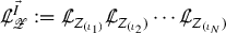denotes an $N^{th}$-order $\ell _{t,u}-$projected Lie derivative operator (see Definition 2.26), and we write when we are not concerned with the structure of $\vec {I}$.

• If $\vec {I} = (\iota _1, \iota _2, \ldots , \iota _N)$, then $\vec {I}_1 + \vec {I}_2 = \vec {I}$ means that $\vec {I}_1 = (\iota _{k_1}, \iota _{k_2}, \ldots , \iota _{k_m})$ and $\vec {I}_2 = (\iota _{k_{m+1}}, \iota _{k_{m+2}}, \ldots , \iota _{k_N})$, where $1 \le m \le N$ and $k_1, k_2, \ldots , k_N$ is a permutation of $1,2,\ldots ,N$.

• Sums such as $\vec {I}_1 + \vec {I}_2 + \cdots + \vec {I}_M = \vec {I}$ have an analogous meaning.

• ${\mathcal {P}}_u-$tangent operators such as $\mathscr {P}^{\vec {I}}$ are defined analogously, except in this case we have $\iota _1, \iota _2, \ldots , \iota _N \in \lbrace 1,2 \rbrace$. We write $\mathscr {P}^N$ rather than $\mathscr {P}^{\vec {I}}$ when we are not concerned with the structure of $\vec {I}$, and we sometimes omit the superscript when $N=1$.

Definition 8.8

(Sets of commutation $\mathscr {Z}$ multi-indices) We define ${\mathcal {I}}_*^{N;M}$ to be the set of $\mathscr {Z}$-multi-indices $\vec {I}$ such that i) $|\vec {I}| = N$, ii) $\mathscr {Z}^{\vec {I}}$ contains at least one factor belonging to $\mathscr {P}= \lbrace L, Y\rbrace$, and iii) $\mathscr {Z}^{\vec {I}}$ contains precisely M factors of $\breve{X}$.

We define ${\mathcal {I}}_*^{N;\le M}$ in the same way, except we replace iii) with iii)’: $\mathscr {Z}^{\vec {I}}$ contains no more than M factors of $\breve{X}$.

Lemma 8.9

[23, Lemma 5.1; Preliminary identities for commuting $Z \in \mathscr {Z}$ with ] For each $\mathscr {Z}$-multi-index $\vec {I}$ and each integer $n \ge 1$, the following commutator identity, correct up to constant factors on the RHS, holds for all type $\ell _{t,u}$-tangent tensorfields $\xi$:

(8.14a)

Moreover, for each $\mathscr {Z}$-multi-index $\vec {I}$, the following commutator identity, correct up to constant factors on the RHS, holds for all symmetric type $\ell _{t,u}$-tangent tensorfields $\xi$:

(8.14b)

Finally, for each $\mathscr {Z}$-multi-index $\vec {I}$, the following commutator identities, correct up to constant factors on the RHS, hold for all scalar functions f:

(8.15a)

(8.15b)

In (8.14a)–(8.15b), we have omitted all tensorial contractions to condense the presentation.

Lemma 8.10

[23, Lemma 5.2; Preliminary Lie derivative commutation identities] Let $\vec {I} = (\iota _1,\iota _2,\ldots , \iota _N)$ be an $N^{th}$-order $\mathscr {Z}$-multi-index, let f be a scalar function, and let $\xi$ be a type $\ell _{t,u}$-tangent tensorfield with $m + n \ge 1$. Let $i_1,i_2,\ldots ,i_N$ be any permutation of $1,2,\ldots ,N$ and let $\vec {I}' = (\iota _{i_1},\iota _{i_2},\ldots , \iota _{i_N})$. Then, up to omitted constant factors on the RHS, we have

In (8.16a)–(8.16b), $\vec {I}_1 + \vec {I}_2 + \iota _{k_1} + \iota _{k_2} = \vec {I}$ means that $\vec {I}_1 = (\iota _{k_3}, \iota _{k_4}, \ldots , \iota _{k_m})$ and $\vec {I}_2 = (\iota _{k_{m+1}}, \iota _{k_{m+2}}, \ldots , \iota _{k_N})$, where $k_1, k_2, \ldots , k_N$ is a permutation of $1,2,\ldots ,N$. In particular, $|\vec {I}_1| + |\vec {I}_2| = N-2$.

8.5.2 Commutator estimates

We now provide the main estimates of Sect. 8.5.

Lemma 8.11

(Commutator estimates) Assume that $1 \le N \le 20$ and $0 \le M \le \min \lbrace N,2 \rbrace$. Let $\vec {I}$ be a multi-index belonging to the set ${\mathcal {I}}_*^{N+1;M}$ from Definition 8.8 and let $\vec {I}'$ be any permutation of $\vec {I}$. Then the following commutator estimates hold:

$$\begin{aligned} \left| \mathscr {Z}^{\vec {I}} f - \mathscr {Z}^{\vec {I}'} f \right|&\lesssim \left| \left( \begin{array}{lr} \mathscr {Z}_{**}^{[1,\lceil N/2 \rceil ];\le (M-1)_+} \underline{\upgamma } \\ \mathscr {Z}_{*}^{[1,\lceil N/2 \rceil ];\le (M-1)_+} \upgamma \end{array} \right) \right| \left| \mathscr {Z}_{**}^{[1,N];\le M} f \right| \nonumber \\&\quad + \underbrace{ \left| \mathscr {Z}_{**}^{[1,N];\le (M-1)_+} f \right| }_{\hbox { Absent if}\ M=0} \nonumber \\&\quad + \left| \mathscr {Z}_{**}^{[1,\lfloor N/2 \rfloor ];\le M} f \right| \left| \left( \begin{array}{lr} \mathscr {Z}_{**}^{[1,N];\le (M-1)_+} \underline{\upgamma } \\ \mathscr {Z}_{*}^{[1,N];\le M} \upgamma \end{array} \right) \right| , \end{aligned}$$

(8.17)

where $(M-1)_+ := \max \lbrace M-1,0 \rbrace$.

Moreover, if $1 \le N \le 19$ and $0 \le M \le \min \lbrace N,2 \rbrace$, then

(8.18a)

(8.18b)

Finally, if $\xi$ is an $\ell _{t,u}$-tangent one-form or a type $\ell _{t,u}$-tangent tensorfield, $1 \le N \le 19$, $0 \le M \le \min \lbrace N,2 \rbrace$, and $\vec {I} \in {\mathcal {I}}_*^{N+1;M}$, then

(8.19a)

(8.19b)

(8.19c)

Proof

See Sect. 8.2 for some comments on the analysis.

Proof of (8.17): We will bound the products on RHS (8.16a) on a case by case basis. Let $M'$ be the number of factors of $\breve{X}$ in $\mathscr {Z}^{\vec {I}_2}$. Note that $M' \le M$ in view of the summation constraint $\vec {I}_1 + \vec {I}_2 + \iota _{k_1} + \iota _{k_2} = \vec {I}$ on RHS (8.16a).

Case i): $M'=M$ and $|\vec {I}_2| \in [\lfloor N/2 \rfloor ,N-1]$. Clearly . To bound , where $|\vec {I}_1| \in [0,\lfloor (N-1)/2 \rfloor ]$, we note that since $M'=M$, it must be that comprises only ${\mathcal {P}}_u$-tangent vectorfield factors and that $(Z_{(\iota _{k_1})}, Z_{(\iota _{k_2})}) = (L,Y)$. Hence, from (8.10), we have . In particular, the product under consideration is bounded by the first product on RHS (8.17).

Case ii): $M'=M$ and $|\vec {I}_2| \in [0,\lfloor N/2 \rfloor - 1]$. A slight modification of the argument from Case i) yields that is bounded by the last product on RHS (8.17).

We note that we have now proved inequality (8.17) in the case $M=0$, and it holds without the second term on the RHS [as is stated in (8.17)].

Case iii): $1 \le M \le 2$, $M'\le M-1$, and $|\vec {I}_2| \in [\lfloor N/2 \rfloor ,N-1]$. Clearly . Since $|\vec {I}_1| \in [0,\lfloor (N-1)/2 \rfloor ]$, we can bound in the norm $\Vert \cdot \Vert _{L^{\infty }(\Sigma _t^u)}$ by $\lesssim 1$ with the help of the pointwise estimates of Lemma 8.6 and the bootstrap assumptions. It follows that is bounded by the second term on RHS (8.17).

Case iv): $1 \le M \le 2$, $M'\le M-1$, $|\vec {I}_2| \in [0,\lfloor N/2 \rfloor - 1]$, and $1 \le N \le 4$. Since N is small, the same arguments given in Case iii) apply.

Case v): $1 \le M \le 2$, $M'\le M-1$, $|\vec {I}_2| \in [0,\lfloor N/2 \rfloor - 1]$, and $5 \le N \le 20$. Clearly . To bound , we start with the sub-case in which either $Z_{(\iota _{k_1})} = \breve{X}$ or $Z_{(\iota _{k_2})} = \breve{X}$. In view of the summation constraint $\vec {I}_1 + \vec {I}_2 + \iota _{k_1} + \iota _{k_2} = \vec {I}$, we see that it suffices to bound and . Since $N \ge 5$ and $|\vec {I}_1| \in [\lceil N/2 \rceil ,N-1]$, we have $|\vec {I}_1| \ge 3$. Thus, since $M \le 2$, at least 2 vectorfield factors in the operator must be ${\mathcal {P}}_u$-tangent. In particular, . We can therefore use (8.11c) with $M-1$ in the role of M to deduce . It follows that is bounded by the last product on RHS (8.17) as desired. In the remaining sub-case, we have $(Z_{(\iota _{k_1})},Z_{(\iota _{k_2})}) = (L, Y)$. Thus, using (8.10), we see that . It follows that is bounded by the last product on RHS (8.17).

Proof of (8.18a) and (8.18b): These estimates can be proved by combining arguments similar to the ones we used to prove (8.17) with the commutation identities (8.15a)–(8.15b), the estimates (8.8a) and (8.8b), and Lemma 8.2; we omit the details.

Proof of (8.19a), (8.19b) and (8.19c): The proofs of these estimates are similar to the proof of (8.17) and are based on the commutation identities (8.14a)–(8.14b) and (8.16b), the estimates (8.8a) and (8.8b), and Lemma 8.3. We omit the details, noting only that the right-hand side of (8.19a) involves one more derivative of $\underline{\upgamma }$ and $\upgamma$ compared to the estimate (8.17); the reason is that we use the estimate (8.3a) when bounding the terms on RHS (8.16b), which leads to the presence of one additional derivative on . $\square$

Corollary 8.12

If $1 \le N \le 20$, $0 \le M \le \min \lbrace N,2 \rbrace$, and $\Psi \in \lbrace {\mathcal {R}}_{(+)},{\mathcal {R}}_{(-)},v^2 \rbrace$, then

(8.20)

Proof

See Sect. 8.2 for some comments on the analysis. We start by decomposing . Lemma 8.3 implies that is $\lesssim$ the first term on RHS (8.20). To deduce  (8.20), we use the commutator estimate (8.18b) with $f=\Psi$ and $N-1$ in the role of N and the bootstrap assumptions. $\square$

8.6 Transport inequalities and strict improvements of the auxiliary bootstrap assumptions

In the next proposition, we use the previous estimates to derive transport inequalities for the eikonal function quantities and strict improvements of the auxiliary bootstrap assumptions of Sect. 7.5

Proposition 8.13

(Transport inequalities and strict improvements of the auxiliary bootstrap assumptions) The following estimates hold.

Transport inequalities for the eikonal function quantities.

• Transport inequalities for $\upmu$. The following pointwise estimate holds:

  $$\begin{aligned} \left| L\upmu \right|&\lesssim \left| \mathscr {Z}\vec {\Psi }\right| . \end{aligned}$$

  (8.21a)

  Moreover, for $1 \le N \le 20$ and $0 \le M \le \min \lbrace N-1,1 \rbrace$, we have

  $$\begin{aligned} \left| L\mathscr {Z}_{*}^{N;M} \upmu \right| , \, \left| \mathscr {Z}_{*}^{N;M} L\upmu \right|&\lesssim \left| \mathscr {Z}_{*}^{[1,N+1];\le M+1} \vec {\Psi }\right| + \left| \left( \begin{array}{lr} \mathscr {Z}_{**}^{[1,N];\le M}\underline{\upgamma } \\ \mathscr {Z}_{*}^{[1,N];\le M} \upgamma \end{array} \right) \right| . \end{aligned}$$

  (8.21b)

• Transport inequalities for $L_{(Small)}^i$ and . For $0 \le N \le 20$ and $0 \le M \le \min \lbrace N,2 \rbrace$, we have

  

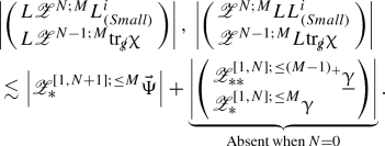  (8.22)

$L^{\infty }$ estimates for $\vec {\Psi }$ and the eikonal function quantities.

• $L^{\infty }$ estimates for $\vec {\Psi }$. The following estimates hold for $M=1,2$:

  $$\begin{aligned} \left\| {\mathcal {R}}_{(+)} \right\| _{L^{\infty }(\Sigma _t^u)}&\le \mathring{\upalpha }+ C \varepsilon , \end{aligned}$$

  (8.23a)
  $$\begin{aligned} \left\| \mathscr {Z}_{*}^{[1,12];\le 2} {\mathcal {R}}_{(+)} \right\| _{L^{\infty }(\Sigma _t^u)}&\le C \varepsilon , \end{aligned}$$

  (8.23b)
  $$\begin{aligned} \left\| \breve{X}^M {\mathcal {R}}_{(+)} \right\| _{L^{\infty }(\Sigma _0^u)}&\le \left\| \breve{X}^M {\mathcal {R}}_{(+)} \right\| _{L^{\infty }(\Sigma _t^u)} + C \varepsilon , \end{aligned}$$

  (8.23c)
  $$\begin{aligned} \left\| \mathscr {Z}^{\le 12 ;\le 2} {\mathcal {R}}_{(-)} \right\| _{L^{\infty }(\Sigma _t^u)}, \, \left\| \mathscr {Z}^{\le 12 ;\le 2} v^2 \right\| _{L^{\infty }(\Sigma _t^u)}&\le C \varepsilon . \end{aligned}$$

  (8.23d)

• $L^{\infty }$ estimates for $\upmu$. The following estimates hold for $M=0,1$:

  $$\begin{aligned} \left\| \breve{X}^M \upmu \right\| _{L^{\infty }(\Sigma _t^u)}&\le \left\| \breve{X}^M \upmu \right\| _{L^{\infty }(\Sigma _0^u)} \nonumber \\&\quad + \mathring{\updelta }_{*}^{-1} \left\| \breve{X}^M \left\{ G_{LL}^0 \breve{X}{\mathcal {R}}_{(+)} \right\} \right\| _{L^{\infty }(\Sigma _0^u)} + C \varepsilon , \end{aligned}$$

  (8.24a)
  $$\begin{aligned} \left\| L\breve{X}^M \upmu \right\| _{L^{\infty }(\Sigma _t^u)}&= \frac{1}{2} \left\| \breve{X}^M \left\{ G_{LL}^0 \breve{X}{\mathcal {R}}_{(+)} \right\} \right\| _{L^{\infty }(\Sigma _0^u)} + {\mathcal {O}}(\varepsilon ), \end{aligned}$$

  (8.24b)
  $$\begin{aligned} \left\| \mathscr {Z}_{**}^{[1,11];\le 1} \upmu \right\| _{L^{\infty }(\Sigma _t^u)}&\le C \varepsilon . \end{aligned}$$

  (8.24c)

  Moreover, we have

  $$\begin{aligned} \left\| \upmu -1 \right\| _{L^{\infty }\left( {\mathcal {P}}_0^{T_{(Boot)}}\right) }&\le C \varepsilon . \end{aligned}$$

  (8.25)

• $L^{\infty }$ estimates for $L_{(Small)}^i$ and $\upchi$. The following estimates hold for $M=1,2$:

  $$\begin{aligned} \left\| L_{(Small)}^1 \right\| _{L^{\infty }(\Sigma _t^u)}&\le C_{\blacklozenge } \mathring{\upalpha }+ C \varepsilon , \end{aligned}$$

  (8.26a)
  $$\begin{aligned} \left\| \mathscr {Z}_{*}^{[1,11];\le 2} L_{(Small)}^1 \right\| _{L^{\infty }(\Sigma _t^u)}&\le C \varepsilon , \end{aligned}$$

  (8.26b)
  $$\begin{aligned} \left\| \mathscr {Z}^{\le 11;\le 2} L_{(Small)}^2 \right\| _{L^{\infty }(\Sigma _t^u)}&\le C \varepsilon , \end{aligned}$$

  (8.26c)
  $$\begin{aligned} \left\| \breve{X}^M L_{(Small)}^1 \right\| _{L^{\infty }(\Sigma _t^u)}&\le \left\| \breve{X}^M L_{(Small)}^1 \right\| _{L^{\infty }(\Sigma _0^u)} + C \varepsilon , \end{aligned}$$

  (8.26d)
  

  (8.27)

$L^{\infty }$ estimates for $\varOmega$.

The following estimates hold:

$$\begin{aligned} \left\| \mathscr {Z}^{\le 12;\le 2} \varOmega \right\| _{L^{\infty }(\Sigma _t^u)}&\le C \varepsilon . \end{aligned}$$

(8.28)

Proof

See Sect. 8.2 for some comments on the analysis. Throughout this proof, we refer to the data-size assumptions of Sect. 7.1, the estimates of Lemma 7.4, and the assumption (7.20) as the “conditions on the data.”

Proof of (8.28): The bootstrap assumptions imply $\left\| \mathscr {P}^{\le 12} \varOmega \right\| _{L^{\infty }(\Sigma _t^u)} \le \varepsilon$, which is a special case of (8.28). To prove (8.28) for $\left\| \mathscr {Z}^{\le 12;1} \varOmega \right\| _{L^{\infty }(\Sigma _t^u)}$, we use (2.40) and (2.8c) to deduce the identity $\breve{X}\varOmega = - \upmu L\varOmega$. Applying $\mathscr {P}^{\le 11}$ to both sides and using the bootstrap assumptions, we deduce $\left\| \mathscr {P}^{\le 11} \breve{X}\varOmega \right\| _{L^{\infty }(\Sigma _t^u)} \lesssim \varepsilon$. Next, for $2 \le K \le 12$, we repeatedly use the commutator estimate (8.17) (see Remark 5.4) and the bootstrap assumptions to deduce

$$\begin{aligned} \left| \mathscr {Z}^{\le K;1} \varOmega \right|&\lesssim \left| \mathscr {P}^{[1,K-1]} \breve{X}\varOmega \right| + \left| \mathscr {P}^{\le K-1} \varOmega \right| . \end{aligned}$$

(8.29)

We have already shown that the first term on RHS (8.29) is $\lesssim \varepsilon$, while the bootstrap assumptions imply that the second term is $\lesssim \varepsilon$. We have thus shown that we can permute the vectorfield factors in $\mathscr {P}^{\le 11} \breve{X}\varOmega$ up to ${\mathcal {O}}(\varepsilon )$ errors, which yields the desired bound $\left\| \mathscr {Z}^{\le 12;1} \varOmega \right\| _{L^{\infty }(\Sigma _t^u)} \lesssim \varepsilon$. To prove (8.28) for $\left\| \mathscr {Z}^{\le 12;2} \varOmega \right\| _{L^{\infty }(\Sigma _t^u)}$, we apply $\mathscr {P}^{\le 10} \breve{X}$ to the equation $\breve{X}\varOmega = - \upmu L\varOmega$ and use the already proven bound $\left\| \mathscr {Z}^{\le 12;\le 1} \varOmega \right\| _{L^{\infty }(\Sigma _t^u)} \lesssim \varepsilon$ and the bootstrap assumptions to deduce $\left\| \mathscr {P}^{\le 10} \breve{X}\breve{X}\varOmega \right\| _{L^{\infty }(\Sigma _t^u)} \lesssim \varepsilon$. Using this bound, the estimate $\left\| \mathscr {Z}^{\le 12;\le 1} \varOmega \right\| _{L^{\infty }(\Sigma _t^u)} \lesssim \varepsilon$, the commutator estimate (8.17), and the bootstrap assumptions, we can use an argument similar to the one given just below (8.29) in order to arbitrarily permute the vectorfield factors in $\mathscr {P}^{\le 10} \breve{X}\breve{X}\varOmega$ up to ${\mathcal {O}}(\varepsilon )$ errors. This yields (8.28).

Proof of (8.21a) and (8.21b): The estimate (8.21a) follows easily from the bootstrap assumptions and the evolution equation $L\upmu = \mathrm {f}(\upgamma ) \breve{X}\vec {\Psi }+ \mathrm {f}(\underline{\upgamma }) P\vec {\Psi }$, which in turn follows from (2.64) and Lemma 2.56.

We now prove (8.21b). We show only how to obtain the estimates for $\left| L\mathscr {Z}_{*}^{N;M} \upmu \right|$ since the estimates for $\left| \mathscr {Z}_{*}^{N;M} L\upmu \right|$ are simpler in that they do not involve commutator estimates. To proceed, for $1 \le N \le 20$ and $0 \le M \le \min \lbrace N-1,1 \rbrace$, we commute the evolution equation from the previous paragraph with $\mathscr {Z}_{*}^{N;M}$ to deduce the schematic identity

$$\begin{aligned} L\mathscr {Z}_{*}^{N;M} \upmu&= [L, \mathscr {Z}_{*}^{N;M}] \upmu + \mathscr {Z}_{*}^{N;M} \left\{ \mathrm {f}(\upgamma ) \breve{X}\vec {\Psi }+ \mathrm {f}(\underline{\upgamma }) P\vec {\Psi }\right\} . \end{aligned}$$

(8.30)

To bound the second term on RHS (8.30) by $\lesssim$ RHS (8.21b), we use the bootstrap assumptions. To derive $\left| [L, \mathscr {Z}_{*}^{N;M}] \upmu \right| \lesssim \text{ RHS }$ (8.21b) , we use the commutator estimate (8.17) with $f = \upmu$ and the bootstrap assumptions.

Proof of (8.22) for $L\mathscr {Z}^{N;M} L_{(Small)}^i$ and $\mathscr {Z}^{N;M} LL_{(Small)}^i$: From (2.65) and Lemma 2.56, we have . For $0 \le N \le 20$ and $0 \le M \le \min \lbrace N,2 \rbrace$, we commute this equation with $\mathscr {Z}^{N;M}$ to obtain

(8.31)

To bound the second term on RHS (8.31) by $\lesssim \text{ RHS }$ (8.22), we use (8.6b)–(8.6c), (8.8a)–(8.8b), and the bootstrap assumptions. To deduce that $\left| [L, \mathscr {Z}^{N;M}] L_{(Small)}^i \right| \lesssim \text{ RHS }$ (8.22), we use (8.17) with $f = L_{(Small)}^i$ and the bootstrap assumptions.

Proof of (8.22) for and : We apply $L$ to (2.75a) and use the schematic identity (see (2.61), (2.73c), and Lemma 2.56) to deduce , where . Applying $\mathscr {Z}^{N-1;M}$ to this identity and using Lemmas 8.4 and 8.5 and the bootstrap assumptions, we find that  (8.22), where the operator $\mathscr {Z}_*^{N+1;M}$ acting on $L_{(Small)}^a$ contains a factor of $L$. Arguing as in our proof of the bound for the commutator term on RHS (8.31), we commute the factor of $L$ so that it acts last, thereby obtaining $\sum _{a=1}^2 \left| \mathscr {Z}_*^{N+1;M} L_{(Small)}^a \right| \lesssim \sum _{a=1}^{2}\left| L\mathscr {Z}^{N;M} L_{(Small)}^a \right| + \text{ RHS }$ (8.22). Moreover, we showed in the previous paragraph that $\sum _{a=1}^{2}\left| L\mathscr {Z}^{N;M} L_{(Small)}^a \right| \lesssim \text{ RHS }$ (8.22), which completes our proof of the estimate (8.22) for . Using the commutator estimate (8.17) with , (8.8c), and the bootstrap assumptions, we commute the factor of $L$ so that it acts last, which yields the same estimate for .

Proof of an intermediate estimate: As an intermediate step, we now show that

$$\begin{aligned} \left| \left( \begin{array}{lr} \mathscr {Z}_{**}^{[1,11];0} \upmu \\ \mathscr {Z}_{*}^{[1,11];\le 1} L_{(Small)}^1 \\ \mathscr {Z}^{\le 11;\le 1} L_{(Small)}^2 \end{array} \right) \right| (t,u,\vartheta )&\lesssim \varepsilon . \end{aligned}$$

(8.32)

We set $q(t,u,\vartheta ) := \text{ LHS }$ (8.32). Since $L= \frac{\partial }{\partial t}$, we can use (8.21b)–(8.22) and the bootstrap assumptions and integrate as in (8.7) to deduce $q(t,u,\vartheta ) \le q(0,u,\vartheta ) + C \int _{s=0}^t q(s,u,\vartheta ) \, ds + C \varepsilon$, where $C \varepsilon$ comes from the terms $\left| \mathscr {Z}_{*}^{[1,12];\le 1} \vec {\Psi }\right|$ on RHSs (8.21b) and (8.22), which are $\lesssim \varepsilon$. The conditions on the data imply that $q(0,u,\vartheta ) \le C \varepsilon$. Hence, Gronwall’s inequality and our assumption $t < T_{(Boot)}\le 2 \mathring{\updelta }_{*}^{-1}$ yield $q(t,u,\vartheta ) \lesssim \varepsilon \exp (C \mathring{\updelta }_{*}^{-1}) \lesssim \varepsilon$ as desired.

Proof of (8.23a)–(8.23d): Using (2.76a), (2.40), Corollary 2.52, Lemma 2.56, the identity (2.85a), and the schematic relation $L\upmu = \mathrm {f}(\underline{\upgamma }) P\vec {\Psi }+ \mathrm {f}(\upgamma ) \breve{X}\vec {\Psi }$ (which follows from (2.64) and Lemma 2.56), we write the wave equations (2.8a) and (2.22) verified by $\Psi \in \lbrace {\mathcal {R}}_{(+)},{\mathcal {R}}_{(-)},v^2 \rbrace$ in the following schematic form:

(8.33)

We now show that⁴¹

$$\begin{aligned} \left| L\mathscr {Z}_{*}^{[2,11];1} \breve{X}\Psi \right| \lesssim \left| \mathscr {Z}_{*}^{[2,11];1} \breve{X}\Psi \right| + \varepsilon . \end{aligned}$$

(8.34)

To derive (8.34), we first apply $\mathscr {Z}_{*}^{[2,11];1}$ to (8.33). Using the bootstrap assumptions and the already proven estimates (8.28) and (8.32) [to bound the derivatives of the terms $L_{(Small)}^1$ and $L_{(Small)}^2$ found in the factor $P\upgamma$ on RHS (8.33)], we deduce . To finish the proof of (8.34), we must bound the commutator term $\left| [L\mathscr {Z}_{*}^{[2,11];1}, \mathscr {Z}_{*}^{[2,11];1} L] \breve{X}\Psi \right|$ To this end, we use the commutator estimate (8.17) with $f = \breve{X}\Psi ,2 \le N \le 11$, and $M=1$, and the bootstrap assumptions, which yield the estimate $\left| [L\mathscr {Z}_{*}^{[2,11];1}, \mathscr {Z}_{*}^{[2,11];1} L] \breve{X}\Psi \right| \lesssim \left| \mathscr {Z}_{**}^{[1,11];\le 1} \breve{X}\Psi \right| \lesssim \left| \mathscr {Z}_{**}^{[2,11];1} \breve{X}\Psi \right| + \varepsilon$, where we bounded the last factor on RHS (8.17) as follows: $\left| \left( \begin{array}{lr} \mathscr {Z}_{**}^{[1,11];0} \underline{\upgamma } \\ \mathscr {Z}_{*}^{[1,11];\le 1} \upgamma \end{array} \right) \right| \lesssim 1$. We have therefore proved (8.34). We now integrate inequality (8.34) along the integral curves of $L$ as in (8.7), use the conditions on the data, and apply Gronwall’s inequality in $\left| \mathscr {Z}_{*}^{[2,11];1} \breve{X}\Psi \right|$ to deduce $\left| \mathscr {Z}_{*}^{[2,11];1} \breve{X}\Psi \right| \lesssim \varepsilon$. Using this bound, the commutator estimate (8.17) with $M=2$, and the bootstrap assumptions, we use a commutator argument similar to the one surrounding Eq. (8.29), which allows us to arbitrarily permute the vectorfield factors in the expression $\mathscr {Z}_{*}^{[2,11];1} \breve{X}\Psi$ up to ${\mathcal {O}}(\varepsilon )$ errors. This yields $\left\| \mathscr {Z}_{*}^{[1,12];2} \vec {\Psi }\right\| _{L^{\infty }(\Sigma _t^u)} \lesssim \varepsilon$. Also considering the bootstrap assumption ($\mathbf {BA}(\vec {\Psi },\varOmega ) \ \mathbf {FUND}$), we see that we have proved (8.23b).

To prove (8.23a), we first note that the bootstrap assumption ($\mathbf {BA}(\vec {\Psi },\varOmega ) \ \mathbf {FUND}$) implies $\left| L{\mathcal {R}}_{(+)} \right| \le \varepsilon$. From this bound and the fundamental theorem of calculus [as in (8.7)], we deduce that $\left| {\mathcal {R}}_{(+)} \right| (t,u,\vartheta ) \le \left| {\mathcal {R}}_{(+)} \right| (0,u,\vartheta ) + C \varepsilon$. From this bound and the conditions on the data, we conclude (8.23a). Similar reasoning yields (8.23c) and the bounds $\left\| \breve{X}^{\le 2} {\mathcal {R}}_{(-)} \right\| _{L^{\infty }(\Sigma _t^u)} \lesssim \varepsilon$ and $\left\| \breve{X}^{\le 2} v^2 \right\| _{L^{\infty }(\Sigma _t^u)} \lesssim \varepsilon$. Combining these bounds with ($\mathbf {BA}(\vec {\Psi },\varOmega ) \ \mathbf {FUND}$) and the bound $\left\| \mathscr {Z}_{*}^{[1,12];\le 2} \vec {\Psi }\right\| _{L^{\infty }(\Sigma _t^u)} \lesssim \varepsilon$ proved above, we conclude (8.23d).

Proof of (8.24c), (8.26a) (8.26b), (8.26c), (8.26d), and (8.27): We define $q(t,u,\vartheta ) := \left| \left( \begin{array}{lr} \mathscr {Z}_{**}^{[1,11];\le 1} \upmu \\ \mathscr {Z}_{*}^{[1,11];\le 2} L_{(Small)}^1 \\ \mathscr {Z}^{\le 11;\le 2} L_{(Small)}^2 \end{array} \right) \right| (t,u,\vartheta )$. Arguing as in our proof of (8.32), we deduce $q(t,u,\vartheta ) \le q(0,u,\vartheta ) + C \int _{s=0}^t q(s,u,\vartheta ) \, ds + C \varepsilon ,$ where the $C \varepsilon$ term comes from the terms $\left| \mathscr {Z}_{*}^{[1,12];\le 2} \vec {\Psi }\right|$ on RHSs (8.21b) and (8.22), which are $\lesssim \varepsilon$ in view of the already proven estimates (8.23b) and (8.23d). The conditions on the data imply that $q(0,u,\vartheta ) \le C \varepsilon$. Hence, from Gronwall’s inequality and the assumption $t < T_{(Boot)}\le 2 \mathring{\updelta }_{*}^{-1}$, we conclude $q(t,u,\vartheta ) \lesssim \varepsilon \exp (C \mathring{\updelta }_{*}^{-1}) \lesssim \varepsilon$, which yields (8.24c), (8.26b), and (8.26c).

The estimate (8.27) then follows as a consequence of inequality (8.8c) and the estimates (8.23b), (8.23d), (8.24c), (8.26b), and (8.26c).

To prove (8.26a), we first use (8.26b) to deduce $\left| LL_{(Small)}^1 \right| \lesssim \varepsilon$. Integrating along the integral curves of $L$, we deduce that $\left| L_{(Small)}^1 \right| (t,u,\vartheta ) \le \left| L_{(Small)}^1 \right| (0,u,\vartheta ) + C \varepsilon$. In view of the conditions on the data, we find that $\left\| L_{(Small)}^1 \right\| _{L^{\infty }(\Sigma _t^u)} \le C_{\blacklozenge } \mathring{\upalpha }+ C \varepsilon$, which yields (8.26a). The estimate (8.26d) can be proved using a similar argument.

Proof of (8.25): The estimate (8.25) is a trivial consequence of (7.16b) and (7.20).

Proof of (8.24a) and (8.24b): From the evolution Eq. (2.64), Lemma 2.56, the commutator estimate (8.17) with $f = \upmu$, the estimates (8.23b), (8.23d), (8.26b), (8.26c), and (8.24c), and the bootstrap assumptions, we see that for $M=0,1$, we have

$$\begin{aligned} L\breve{X}^M \upmu&= \frac{1}{2} \breve{X}^M \left\{ G_{LL}^0 \breve{X}{\mathcal {R}}_{(+)} \right\} + \breve{X}^M \left\{ \mathrm {f}(\upgamma ) \breve{X}{\mathcal {R}}_{(-)} \right\} + \breve{X}^M \left\{ \mathrm {f}(\upgamma ) \breve{X}v^2 \right\} \nonumber \\&\quad \ \ + \breve{X}^M \left\{ \mathrm {f}(\underline{\upgamma }) P\vec {\Psi }\right\} + [L,\breve{X}^M] \upmu \nonumber \\&= \frac{1}{2} \breve{X}^M \left\{ G_{LL}^0 \breve{X}{\mathcal {R}}_{(+)} \right\} + {\mathcal {O}}(\varepsilon ). \end{aligned}$$

(8.35)

Moreover, from (2.80b), (8.23b), (8.23d), (8.26b), (8.26c), and the bootstrap assumptions, we deduce $L\breve{X}^M \left\{ G_{LL}^0 \breve{X}{\mathcal {R}}_{(+)} \right\} = {\mathcal {O}}(\varepsilon )$. Integrating this estimate along the integral curves of $L$ as in (8.7), we find that $\left\| \breve{X}^M \left\{ G_{LL}^0 \breve{X}{\mathcal {R}}_{(+)} \right\} \right\| _{L^{\infty }(\Sigma _t^u)} = \left\| \breve{X}^M \left\{ G_{LL}^0 \breve{X}{\mathcal {R}}_{(+)} \right\} \right\| _{L^{\infty }(\Sigma _0^u)} + {\mathcal {O}}(\varepsilon )$. From this estimate and (8.35), we conclude (8.24b).

To prove (8.24a), we first argue as in (8.7) to obtain the following inequality for $M=0,1$: $\left| \breve{X}^M \upmu \right| (t,u,\vartheta ) \le \left| \breve{X}^M \upmu \right| (0,u,\vartheta ) + \int _{s=0}^t \left| L\breve{X}^M \upmu \right| (s,u,\vartheta ) \, ds$. Then, using (8.24b) and the assumption $0 \le t < T_{(Boot)}\le 2 \mathring{\updelta }_{*}^{-1}$, we bound the time integral by $\le \mathring{\updelta }_{*}^{-1} \Vert \breve{X}^M \lbrace G_{LL}^0 \breve{X}{\mathcal {R}}_{(+)} \} \Vert _{L^\infty (\Sigma _0^u)} + C \varepsilon$. The desired bound (8.24a) now readily follows from these estimates. $\square$

The following corollary is an immediate consequence of the fact that we have improved the auxiliary bootstrap assumptions of Sect. 7.5 by showing that they hold with $\varepsilon ^{1/2}$ replaced by $C \varepsilon$.

Corollary 8.14

$(\varepsilon ^{1/2}$ can be replaced by $C \varepsilon )$ All prior inequalities whose right-hand sides feature an explicit factor of $\varepsilon ^{1/2}$ remain true with $\varepsilon ^{1/2}$ replaced by $C \varepsilon$.

9 $L^{\infty }$ estimates involving higher transversal derivatives

In Sect. 10, we will derive sharp pointwise estimates for $\upmu$ and some of its derivative. Those estimates play a crucial role in the energy estimates. The proofs of some of the estimates of Sect. 10 rely on the bound $\left\| \breve{X}\breve{X}\upmu \right\| _{L^{\infty }(\Sigma _t^u)} \lesssim ~1$. In this section, we derive this bound and some related ones, some of which are needed to prove it.

9.1 Auxiliary bootstrap assumptions

We make auxiliary bootstrap assumptions on ${\mathcal {M}}_{T_{(Boot)};U_0}$ to simplify the analysis.

Auxiliary bootstrap assumptions involving three transversal derivatives of $\vec {\Psi }$.

We assume that the following inequalities hold for $(t,u) \in [0,T_{(Boot)}) \times [0,U_0]$:

Auxiliary bootstrap assumptions involving two transversal derivatives of $\upmu$. We assume that the following inequalities hold for $(t,u) \in [0,T_{(Boot)}) \times [0,U_0]$:

9.2 The main estimates involving higher-order transversal derivatives

In the next proposition, we provide the main estimates of Sect. 9. The proposition yields, in particular, strict improvements of the bootstrap assumptions of Sect. 9.1.

Proposition 9.1

($L^{\infty }$ estimates involving higher-order transversal derivatives) Under the data-size and bootstrap assumptions of Sects. 7.1-7.5 and 9.1 and the smallness assumptions of Sect. 7.6, the following estimates hold.

$L^{\infty }$ estimates involving three transversal derivatives of $\vec {\Psi }$.

$$\begin{aligned} \left\| L\breve{X}\breve{X}\breve{X}\vec {\Psi }\right\| _{L^{\infty }(\Sigma _t^u)}&\le C \varepsilon , \end{aligned}$$

(9.1)

$$\begin{aligned} \left\| \breve{X}\breve{X}\breve{X}{\mathcal {R}}_{(+)} \right\| _{L^{\infty }(\Sigma _t^u)}&\le \left\| \breve{X}\breve{X}\breve{X}{\mathcal {R}}_{(+)} \right\| _{L^{\infty }(\Sigma _0^u)} + C \varepsilon , \end{aligned}$$

(9.2a)

$$\begin{aligned} \left\| \breve{X}\breve{X}\breve{X}{\mathcal {R}}_{(-)} \right\| _{L^{\infty }(\Sigma _t^u)}, \, \left\| \breve{X}\breve{X}\breve{X}v^2 \right\| _{L^{\infty }(\Sigma _t^u)}&\le C \varepsilon . \end{aligned}$$

(9.2b)

$L^{\infty }$ estimates involving two transversal derivatives of $\upmu$.

$$\begin{aligned} \left\| \breve{X}\breve{X}\upmu \right\| _{L^{\infty }(\Sigma _t^u)}&\le \left\| \breve{X}\breve{X}\upmu \right\| _{L^{\infty }(\Sigma _0^u)} + \mathring{\updelta }_{*}^{-1} \left\| \breve{X}\breve{X}\left\{ G_{LL}^0 \breve{X}{\mathcal {R}}_{(+)} \right\} \right\| _{L^{\infty }(\Sigma _0^u)} + C \varepsilon , \end{aligned}$$

(9.3a)

$$\begin{aligned} \left\| L\breve{X}\breve{X}\upmu \right\| _{L^{\infty }(\Sigma _t^u)}&\le \frac{1}{2} \left\| \breve{X}\breve{X}\left\{ G_{LL}^0 \breve{X}{\mathcal {R}}_{(+)} \right\} \right\| _{L^{\infty }(\Sigma _0^u)} + C \varepsilon . \end{aligned}$$

(9.3b)

Sharp pointwise estimates involving the critical factor $\vec {G}_{LL}$. If $0 \le M \le 2$ and $0 \le s \le t < T_{(Boot)}$, then we have the following estimates:

$$\begin{aligned} \left| \breve{X}^M \vec {G}_{LL}(t,u,\vartheta ) - \breve{X}^M \vec {G}_{LL}(s,u,\vartheta ) \right|&\le C \varepsilon (t - s), \end{aligned}$$

(9.4a)

$$\begin{aligned} \left| \breve{X}^M \left\{ \vec {G}_{LL} \diamond \breve{X}\vec {\Psi }\right\} (t,u,\vartheta ) - \breve{X}^M \left\{ \vec {G}_{LL} \diamond \breve{X}\vec {\Psi }\right\} (s,u,\vartheta ) \right|&\le C \varepsilon (t - s). \end{aligned}$$

(9.4b)

Furthermore, we have

$$\begin{aligned} \left\| G_{LL}^2 \right\| _{L^{\infty }(\Sigma _t^u)}&\le C \varepsilon . \end{aligned}$$

(9.5)

Finally, with $\bar{c}_s' := \frac{d}{d \uprho } c_s(\uprho = 0)$ and under the assumption (7.2), we have

$$\begin{aligned} L\upmu (t,u,\vartheta )&= - \frac{1}{2} \left\{ 1 + {\mathcal {O}}_{\blacklozenge }(\mathring{\upalpha }) \right\} (\bar{c}_s' + 1) \breve{X}{\mathcal {R}}_{(+)}(t,u,\vartheta ) + {\mathcal {O}}(\varepsilon ). \end{aligned}$$

(9.6)

Proof of Proposition 9.1

See Sect. 8.2 for some comments on the analysis. Throughout this proof, we refer to the data-size assumptions of Sect. 7.1, the estimates of Lemma 7.4, and the assumption (7.20) as the “conditions on the data.”

Proof of (9.1)–(9.2b): For $\Psi \in \lbrace {\mathcal {R}}_{(+)},{\mathcal {R}}_{(-)},v^2 \rbrace$, we commute (8.33) with $\breve{X}\breve{X}$ and use Lemmas 8.4 and 8.5, the $L^{\infty }$ estimates of Proposition 8.13, and the auxiliary bootstrap assumptions of Sect. 9.1 to deduce

$$\begin{aligned} \left| L\breve{X}\breve{X}\breve{X}\Psi \right|\le & {} \left| L\breve{X}\breve{X}\breve{X}\Psi - \breve{X}\breve{X}L\breve{X}\Psi \right| + \left| \breve{X}\breve{X}L\breve{X}\Psi \right| \\\lesssim & {} \left| L\breve{X}\breve{X}\breve{X}\Psi - \breve{X}\breve{X}L\breve{X}\Psi \right| + \varepsilon . \end{aligned}$$

Also using (8.17) with $f = \breve{X}\Psi$, we deduce

$$\begin{aligned} \left| L\breve{X}\breve{X}\breve{X}\Psi - \breve{X}\breve{X}L\breve{X}\Psi \right|&\lesssim \left| \mathscr {Z}_{**}^{[1,2];\le 2} \breve{X}\Psi \right| \lesssim \left| \mathscr {Z}_{**}^{[1,3];\le 2} \Psi \right| \lesssim \varepsilon , \end{aligned}$$

(9.7)

where to obtain the next-to-last inequality in (9.7), we have used the fact that operators of the form $\mathscr {Z}_{**}^{[1,2];\le 2}$ cannot contain two factors of $\breve{X}$. We have therefore proved (9.1). The estimates (9.2a)–(9.2b) then follow from integrating along the integral curves of $L$ as in (8.7) and using the estimate (9.1) and the conditions on the data.

Proof of (9.4a)–(9.4b): It suffices to prove that for $M=0,1,2$ and $\imath = 0,1,2$, we have

$$\begin{aligned} \left| L\breve{X}^M G_{LL}^{\imath } \right| , \, \left| L\breve{X}^M \left\{ G_{LL}^{\imath } \breve{X}\Psi _{\imath } \right\} \right|&\lesssim \varepsilon ; \end{aligned}$$

(9.8)

once we have shown (9.8), (9.4a)–(9.4b) then follow from integrating along the integral curves of $L$ from time s to t [in analogy with (8.7)] and using (9.8).

To obtain the estimate (9.8) for $L\breve{X}^M G_{LL}^{\imath }$, we differentiate $G_{LL}^{\imath } = \mathrm {f}(\upgamma )$ [see (2.80b)] with $L\breve{X}^M$ and use the $L^{\infty }$ estimates of Proposition 8.13. To obtain the estimate (9.8) for $L\breve{X}^M \left\{ G_{LL}^{\imath } \breve{X}\Psi _{\imath } \right\}$, we use a similar argument that also relies on (9.1)–(9.2b).

Proof of (9.5): From (2.66), the identity $X^2 = X_{(Small)}^2$ (see Definition 2.38), Lemma 2.39, and Lemma 2.56, we deduce $G_{LL}^2 = \mathrm {f}(\upgamma ) L_{(Small)}^2 + \mathrm {f}(\upgamma ) v^2$. (9.5) now follows from the $L^{\infty }$ estimates of Proposition 8.13.

Proof of (9.6): From (2.12), the definition $\bar{c}_s' := \frac{d}{d \uprho } c_s(\uprho = 0)$, (2.64), (2.67), and Lemma 2.56, we deduce

$$\begin{aligned} L\upmu&= - \frac{1}{2} c_s^{-1} \left\{ c_s^{-1} c_s' + 1 \right\} \breve{X}{\mathcal {R}}_{(+)} + \mathrm {f}(\upgamma ) \breve{X}{\mathcal {R}}_{(-)} + \mathrm {f}(\underline{\upgamma }) P\vec {\Psi }\nonumber \\&= - \frac{1}{2} \left\{ \bar{c}_s' + 1 + \upgamma \mathrm {f}(\upgamma ) \right\} \breve{X}{\mathcal {R}}_{(+)} + \mathrm {f}(\upgamma ) \breve{X}{\mathcal {R}}_{(-)} + \mathrm {f}(\upgamma ) \breve{X}v^2 + \mathrm {f}(\underline{\upgamma }) P\vec {\Psi }. \end{aligned}$$

(9.9)

(9.6) now follows from (7.2), (9.9), and the $L^{\infty }$ estimates of Proposition 8.13, which imply that $- \frac{1}{2} \left\{ \bar{c}_s' \!+\! 1 \!+\! \upgamma \mathrm {f}(\upgamma ) \right\} \breve{X}{\mathcal {R}}_{(+)} \!=\! - \frac{1}{2} \left\{ 1 \!+\! {\mathcal {O}}_{\blacklozenge }(\mathring{\upalpha }) \right\} (\bar{c}_s' \!+\! 1) \breve{X}{\mathcal {R}}_{(+)}(t,u,\vartheta ) \!+\! {\mathcal {O}}(\varepsilon )$ and that the last three products on RHS (9.9) are ${\mathcal {O}}(\varepsilon )$.

Proof of (9.3a)–(9.3b): Using the $L^{\infty }$ estimates of Proposition 8.13, the estimate (9.2b), and the bootstrap assumptions, we can use the same argument that we used to prove (8.35) in the cases $M=0$,1 in order to conclude that (8.35) also holds with $M=2$. The remainder of the proof of (9.3a)–(9.3b) now proceeds as in the proof of (8.24a)–(8.24b) [which is given just below (8.35)], thanks to the availability of the already proven estimates in (9.8). $\square$

10 Sharp estimates for $\upmu$

In this section, we derive sharp pointwise estimates for $\upmu$ and some of its derivatives. These estimates provide much more information than the crude estimates we obtained in Sects. 8 and 9. The sharp estimates play an essential role in our derivation a priori energy estimates (see Sect. 14).

10.1 Definitions and preliminary ingredients in the analysis

Definition 10.1

(Auxiliary quantities used to analyze $\upmu$) We define the following quantities, where $0 \le s \le t$ for those quantities that depend on both s and t : 

$$\begin{aligned} M(s,u,\vartheta ;t)&:= \int _{s'=s}^{s'=t} \left\{ L\upmu (t,u,\vartheta ) - L\upmu (s',u,\vartheta ) \right\} \, ds', \end{aligned}$$

(10.1a)

$$\begin{aligned} \mathring{\upmu }(u,\vartheta )&:= \upmu (s=0,u,\vartheta ), \end{aligned}$$

(10.1b)

$$\begin{aligned} {\widetilde{M}}(s,u,\vartheta ;t)&:= \frac{M(s,u,\vartheta ;t)}{\mathring{\upmu }(u,\vartheta ) - M(0,u,\vartheta ;t)}, \end{aligned}$$

(10.1c)

$$\begin{aligned} \upmu _{(Approx)}(s,u,\vartheta ;t)&:= 1 + \frac{L\upmu (t,u,\vartheta )}{ \mathring{\upmu }(u,\vartheta ) - M(0,u,\vartheta ;t)}s + {\widetilde{M}}(s,u,\vartheta ;t). \end{aligned}$$

(10.1d)

The following quantity $\upmu _{\star }$ captures the worst-case smallness of $\upmu$ along $\Sigma _t^u$. Our high-order energies are allowed to blow up like a positive power of $1/\upmu _{\star }$ as $\upmu _{\star } \rightarrow 0$; see Proposition 14.1.

Definition 10.2

(Definition of $\upmu _{\star }$) We define

$$\begin{aligned} \upmu _{\star }(t,u)&:= \min \lbrace 1, \min _{\Sigma _t^u} \upmu \rbrace . \end{aligned}$$

(10.2)

Lemma 10.3

(First estimates for the auxiliary quantities) The following estimates hold for $(t,u,\vartheta ) \in [0,T_{(Boot)}) \times [0,U_0] \times {\mathbb {T}}$ and $0 \le s \le t$:

In addition, the following pointwise estimates hold:

$$\begin{aligned} \left| L\upmu (t,u,\vartheta ) - L\upmu (s,u,\vartheta ) \right|&\lesssim \varepsilon (t-s), \end{aligned}$$

(10.5)

$$\begin{aligned} |M(s,u,\vartheta ;t)|, |{\widetilde{M}}(s,u,\vartheta ;t)|&\lesssim \varepsilon (t - s)^2, \end{aligned}$$

(10.6)

$$\begin{aligned} \upmu (s,u,\vartheta )&= \left\{ 1 + {\mathcal {O}}_{\blacklozenge }(\mathring{\upalpha }) + {\mathcal {O}}(\varepsilon ) \right\} \upmu _{(Approx)}(s,u,\vartheta ;t). \end{aligned}$$

(10.7)

Proof

(10.3) follows from (7.13a) and (7.20). The estimate (10.5) follows from the mean value theorem and the estimate $\left| LL\upmu \right| \lesssim \varepsilon$, which is a special case of (8.24c). The estimate (10.4) and the estimate (10.6) for M then follow from definition (10.1a) and the estimates (10.3) and (10.5). The estimate (10.6) for ${\widetilde{M}}$ follows from definition (10.1c), the estimate (10.6) for M, and (10.4). To prove (10.7), we first note the following identity, which is a straightforward consequence of Definition 10.1:

$$\begin{aligned} \upmu (s,u,\vartheta ) = \left\{ \mathring{\upmu }(u,\vartheta ) - M(0,u,\vartheta ;t) \right\} \upmu _{(Approx)}(s,u,\vartheta ;t). \end{aligned}$$

(10.8)

From (10.8) and (10.4), we conclude (10.7). $\square$

In deriving certain estimates, we find it convenient to partition various subsets of spacetime into regions where $L\upmu < 0$ (and hence $\upmu$ is decaying) and regions where $L\upmu \ge 0$ (and hence $\upmu$ is not decaying).

Definition 10.4

(Regions of distinct $\upmu$ behavior) For each $t \in [0,T_{(Boot)})$, $s \in [0,t]$, and $u \in [0,U_0]$, we partition

$$\begin{aligned}{}[0,u] \times {\mathbb {T}}&= {^{(+)} \mathcal {V}_{t}^{u}} \cup {^{(-)} \mathcal {V}_{t}^{u}},&\Sigma _s^u&= {^{(+)} \Sigma _{s;t}^{u}} \cup {^{(-)} \Sigma _{s;t}^{u}}, \end{aligned}$$

(10.9)

where⁴²

$$\begin{aligned} {^{(+)} \mathcal {V}_{t}^{u}}&:= \left\{ (u',\vartheta ) \in [0,u] \times {\mathbb {T}} \ | \ \frac{L\upmu (t,u',\vartheta )}{\mathring{\upmu }(u',\vartheta ) - M(0,u',\vartheta ;t)} \ge 0 \right\} , \end{aligned}$$

(10.10a)

$$\begin{aligned} {^{(-)} \mathcal {V}_{t}^{u}}&:= \left\{ (u',\vartheta ) \in [0,u] \times {\mathbb {T}} \ | \ \frac{L\upmu (t,u',\vartheta )}{\mathring{\upmu }(u',\vartheta ) - M(0,u',\vartheta ;t)} < 0 \right\} , \end{aligned}$$

(10.10b)

$$\begin{aligned} {^{(\pm )} \Sigma _{s;t}^{u}}&:= \left\{ (s,u',\vartheta ) \in \Sigma _s^u \ | \ (u',\vartheta ) \in {^{(\pm )} \mathcal {V}_{t}^{u}} \right\} . \end{aligned}$$

(10.10c)

10.2 Sharp pointwise estimates for $\upmu$ and its derivatives

In the next proposition, we provide the sharp pointwise estimates for $\upmu$ that we use to close our energy estimates.

Proposition 10.5

(Sharp pointwise estimates for $\upmu$, $L\upmu$, and $\breve{X}\upmu )$ The following estimates hold for $(t,u,\vartheta ) \in [0,T_{(Boot)}) \times [0,U_0] \times {\mathbb {T}}$ and $0 \le s \le t$.

Upper bound for $\displaystyle \frac{[L\upmu ]_+}{\upmu }$.

$$\begin{aligned} \left\| \frac{[L\upmu ]_+}{\upmu } \right\| _{L^{\infty }(\Sigma _s^u)}&\le C. \end{aligned}$$

(10.11)

Small $\upmu$ implies $L\upmu$ is negative.

$$\begin{aligned} \upmu (s,u,\vartheta ) \le \frac{1}{4} \implies L\upmu (s,u,\vartheta ) \le - \frac{1}{4} \mathring{\updelta }_{*}, \end{aligned}$$

(10.12)

where $\mathring{\updelta }_{*}> 0$ is defined in (7.1).

Upper bound for $\displaystyle \frac{[\breve{X}\upmu ]_+}{\upmu }$.

$$\begin{aligned} \left\| \frac{[\breve{X}\upmu ]_+}{\upmu } \right\| _{L^{\infty }(\Sigma _s^u)}&\le \frac{C}{\sqrt{T_{(Boot)}- s}}. \end{aligned}$$

(10.13)

Sharp spatially uniform estimates. Consider a time interval $s \in [0,t]$ and define the (t, u-dependent) constant $\upkappa$ by

$$\begin{aligned} \upkappa&:= \sup _{(u',\vartheta ) \in [0,u] \times {\mathbb {T}}} \frac{[L\upmu ]_-(t,u',\vartheta )}{\mathring{\upmu }(u',\vartheta ) - M(0,u',\vartheta ;t)}, \end{aligned}$$

(10.14)

and note that $\upkappa \ge 0$ in view of the estimate (10.4). Then

$$\begin{aligned} \upmu _{\star }(s,u)&= \left\{ 1 + {\mathcal {O}}_{\blacklozenge }(\mathring{\upalpha }) + {\mathcal {O}}(\varepsilon ) \right\} \left\{ 1 - \upkappa s \right\} , \end{aligned}$$

(10.15a)

$$\begin{aligned} \left\| [L\upmu ]_- \right\| _{L^{\infty }(\Sigma _s^u)}&= {\left\{ \begin{array}{ll} \left\{ 1 + {\mathcal {O}}_{\blacklozenge }(\mathring{\upalpha }) + {\mathcal {O}}(\varepsilon ^{1/2}) \right\} \upkappa , &{} \text{ if } \upkappa \ge \varepsilon ^{1/2},\\ {\mathcal {O}}(\varepsilon ^{1/2}), &{} \text{ if } \upkappa \le \varepsilon ^{1/2}. \end{array}\right. } \end{aligned}$$

(10.15b)

Furthermore, we have

$$\begin{aligned} \upkappa&\le \left\{ 1 + {\mathcal {O}}_{\blacklozenge }(\mathring{\upalpha }) + {\mathcal {O}}(\varepsilon ) \right\} \mathring{\updelta }_{*}. \end{aligned}$$

(10.16a)

Moreover, when $u = 1$, we have

$$\begin{aligned} \upkappa&= \left\{ 1 + {\mathcal {O}}_{\blacklozenge }(\mathring{\upalpha }) + {\mathcal {O}}(\varepsilon ) \right\} \mathring{\updelta }_{*}. \end{aligned}$$

(10.16b)

Sharp estimates when $(u',\vartheta ) \in {^{(+)} \mathcal {V}_{t}^{u}}$. We recall that the set ${^{(+)} \mathcal {V}_{t}^{u}}$ is defined in (10.10a). If $0 \le s_1 \le s_2 \le t$, then the following estimate holds:

$$\begin{aligned} \sup _{(u',\vartheta ) \in {^{(+)} \mathcal {V}_{t}^{u}}} \frac{\upmu (s_2,u',\vartheta )}{\upmu (s_1,u',\vartheta )}&\le C. \end{aligned}$$

(10.17)

In addition, if $s \in [0,t]$ and ${^{(+)} \Sigma _{s;t}^{u}}$ is as defined in (10.10c), then

$$\begin{aligned} \inf _{{^{(+)} \Sigma _{s;t}^{u}}} \upmu&\ge 1 - C_{\blacklozenge } \mathring{\upalpha }- C \varepsilon . \end{aligned}$$

(10.18)

Moreover, if $s \in [0,t]$, then

$$\begin{aligned} \left\| \frac{[L\upmu ]_-}{\upmu } \right\| _{L^{\infty }({^{(+)} \Sigma _{s;t}^{u}})}&\le C \varepsilon . \end{aligned}$$

(10.19)

Sharp estimates when $(u',\vartheta ) \in {^{(-)} \mathcal {V}_{t}^{u}}$. Assume that the set ${^{(-)} \mathcal {V}_{t}^{u}}$ defined in (10.10b) is non-empty, let $\upkappa$ be as in (10.14), and note that $\upkappa > 0$ when ${^{(-)} \mathcal {V}_{t}^{u}}$ is non-empty. Then there exists a constant $C > 0$ such that

$$\begin{aligned} \mathop {\sup _{0 \le s_1 \le s_2 \le t}}_{(u',\vartheta ) \in {^{(-)} \mathcal {V}_{t}^{u}}} \frac{\upmu (s_2,u',\vartheta )}{\upmu (s_1,u',\vartheta )}&\le 1 + C \varepsilon . \end{aligned}$$

(10.20)

Furthermore, if $s \in [0,t]$ and ${^{(-)} \Sigma _{s;t}^{u}}$ is as defined in (10.10c), then

$$\begin{aligned} \left\| [L\upmu ]_+ \right\| _{L^{\infty }({^{(-)} \Sigma _{s;t}^{u}})}&\le C \varepsilon . \end{aligned}$$

(10.21)

Finally, there exist constants $C_{\blacklozenge } > 0$ and $C > 0$ such that if $0 \le s \le t$, then

$$\begin{aligned} \left\| [L\upmu ]_- \right\| _{L^{\infty }({^{(-)} \Sigma _{s;t}^{u}})}&\le {\left\{ \begin{array}{ll} \left\{ 1 + C_{\blacklozenge } \mathring{\upalpha }+ C \varepsilon ^{1/2} \right\} \upkappa , &{} \text{ if } \upkappa \ge \varepsilon ^{1/2}, \\ C \varepsilon ^{1/2}, &{} \text{ if } \upkappa \le \varepsilon ^{1/2}. \end{array}\right. } \end{aligned}$$

(10.22)

Approximate time-monotonicity of $\upmu _{\star }^{-1}(s,u)$. There exist constants $C_{\blacklozenge } > 0$ and $C > 0$ such that if $0 \le s_1 \le s_2 \le t$, then

$$\begin{aligned} \upmu _{\star }^{-1}(s_1,u)&\le \{1 + C_{\blacklozenge } \mathring{\upalpha }+ C \varepsilon \} \upmu _{\star }^{-1}(s_2,u). \end{aligned}$$

(10.23)

Proof

See Sect. 8.2 for some comments on the analysis.

Proof of (10.11): We may assume that $L\upmu (s,u,\vartheta ) > 0$ since otherwise (10.11) is trivial. Then by (10.5), for $0 \le s' \le s \le t < T_{(Boot)}\le 2 \mathring{\updelta }_{*}^{-1}$, we have that $L\upmu (s',u,\vartheta ) \ge L\upmu (s,u,\vartheta ) - C \varepsilon (s-s') \ge - C \varepsilon$. Integrating this estimate with respect to $s'$ starting from $s'=0$ and using (10.3), we find that $\upmu (s,u,\vartheta ) \ge 1 - C_{\blacklozenge } \mathring{\upalpha }- C \varepsilon$ and thus $1/\upmu (s,u,\vartheta ) \le 1 + C_{\blacklozenge } \mathring{\upalpha }+ C \varepsilon$. Also using the bound $\left| L\upmu (s,u,\vartheta ) \right| \le C$ proved in (8.24b), we conclude the desired estimate.

Proof of (10.12): By (10.5), for $0 \le s \le t < T_{(Boot)}\le 2 \mathring{\updelta }_{*}^{-1}$, we have that $L\upmu (s,u,\vartheta ) = L\upmu (0,u,\vartheta ) + {\mathcal {O}}(\varepsilon )$. Integrating this estimate with respect to s starting from $s=0$ and using (10.3), we find that $\upmu (s,u,\vartheta ) = 1 + {\mathcal {O}}_{\blacklozenge }(\mathring{\upalpha }) + {\mathcal {O}}(\varepsilon ) + s L\upmu (0,u,\vartheta )$. Again using (10.5) to deduce that $L\upmu (0,u,\vartheta ) = L\upmu (s,u,\vartheta ) + {\mathcal {O}}(\varepsilon )$, we find that $\upmu (s,u,\vartheta ) = 1 + {\mathcal {O}}_{\blacklozenge }(\mathring{\upalpha }) + {\mathcal {O}}(\varepsilon ) + s L\upmu (s,u,\vartheta )$. It follows that whenever $\upmu (s,u,\vartheta ) < 1/4$, we have $L\upmu (s,u,\vartheta )< - \frac{1}{2} \left\{ 3/4 + {\mathcal {O}}_{\blacklozenge }(\mathring{\upalpha }) + {\mathcal {O}}(\varepsilon ) \right\} \mathring{\updelta }_{*}< - \frac{1}{4} \mathring{\updelta }_{*}$ as desired.

Proof of (10.16a) and (10.16b): We prove only (10.16a) since (10.16b) follows from nearly identical arguments. From (7.2), (9.9), (10.4), (10.5), and the $L^{\infty }$ estimates of Proposition 8.13, we have

(10.24)

From (10.24) and definitions (7.1) and (10.14), we conclude that $\upkappa \le \left\{ 1 + {\mathcal {O}}_{\blacklozenge }(\mathring{\upalpha }) \right\} \mathring{\updelta }_{*}+ {\mathcal {O}}(\varepsilon ) = \left\{ 1 + {\mathcal {O}}_{\blacklozenge }(\mathring{\upalpha }) + {\mathcal {O}}(\varepsilon ) \right\} \mathring{\updelta }_{*}$ as desired.

Proof of (10.15a) and (10.23): We first prove (10.15a). We start by establishing the following preliminary estimate for the crucial quantity $\upkappa = \upkappa (t,u)$ [see (10.14)]:

$$\begin{aligned} t \upkappa < 1. \end{aligned}$$

(10.25)

We may assume that $\upkappa > 0$ since otherwise the estimate is trivial. To proceed, we use (10.1d), (10.4), (10.6), and (10.8) to deduce that the following estimate holds for $(s,u',\vartheta ) \in [0,t] \times [0,u] \times {\mathbb {T}}$:

(10.26)

Setting $s=t$ in Eq. (10.26), taking the min of both sides over $(u',\vartheta ) \in [0,u] \times {\mathbb {T}}$, and appealing to definitions (10.2) and (10.14), we deduce that $\upmu _{\star }(t,u) = \left\{ 1 + {\mathcal {O}}_{\blacklozenge }(\mathring{\upalpha }) + {\mathcal {O}}(\varepsilon ) \right\} (1-\upkappa t)$. Since $\upmu _{\star }(t,u) > 0$ by ($\mathbf {BA} \ \upmu > 0$), we conclude (10.25).

Having established the preliminary estimate, we now take the min of both sides of (10.26) over $(u',\vartheta ) \in [0,u] \times {\mathbb {T}}$, use the estimate (8.25), and appeal to definitions (10.2) and (10.14) to obtain:

$$\begin{aligned} \min _{(u',\vartheta ) \in [0,u] \times {\mathbb {T}}} \upmu (s,u',\vartheta )&= \left\{ 1 + {\mathcal {O}}_{\blacklozenge }(\mathring{\upalpha }) + {\mathcal {O}}(\varepsilon ) \right\} \left\{ 1 - \upkappa s + {\mathcal {O}}(\varepsilon ) (t-s)^2 \right\} . \end{aligned}$$

(10.27)

We will show that the terms in the second braces on RHS (10.27) satisfy

$$\begin{aligned} 1 - \upkappa s + {\mathcal {O}}(\varepsilon ) (t-s)^2&= (1 + \mathrm {f}(s,u;t)) \left\{ 1 - \upkappa s \right\} , \end{aligned}$$

(10.28)

where

$$\begin{aligned} \mathrm {f}(s,u;t)&= {\mathcal {O}}(\varepsilon ). \end{aligned}$$

(10.29)

The desired estimate (10.15a) then follows easily from (10.27)–(10.29) and definition (10.2). To prove (10.29), we first use (10.28) to solve for $\mathrm {f}(s,u;t)$:

$$\begin{aligned} \mathrm {f}(s,u;t) = \frac{{\mathcal {O}}(\varepsilon ) (t-s)^2 }{ 1 - \upkappa s } = \frac{{\mathcal {O}}(\varepsilon ) (t-s)^2 }{ 1 - \upkappa t + \upkappa (t-s) }. \end{aligned}$$

(10.30)

We start by considering the case $\upkappa \le (1/4) \mathring{\updelta }_{*}$. Since $0 \le s \le t < T_{(Boot)}\le 2 \mathring{\updelta }_{*}^{-1}$, the denominator in the middle expression in (10.30) is $\ge 1/2$, and the desired estimate (10.29) therefore follows easily whenever $\varepsilon$ is sufficiently small. In remaining case, we have $\upkappa > (1/4) \mathring{\updelta }_{*}$. Using (10.25), we deduce that RHS (10.30) $\displaystyle \le \frac{1}{\upkappa } {\mathcal {O}}(\varepsilon ) (t-s) \le C \varepsilon \mathring{\updelta }_{*}^{-2} \lesssim \varepsilon$ as desired.

Inequality (10.23) then follows as a simple consequence of (10.15a).

Proof of (10.15b) and (10.22): To prove (10.15b), we first use (10.5) to deduce that for $0 \le s \le t < T_{(Boot)}\le 2 \mathring{\updelta }_{*}^{-1}$ and $(u',\vartheta ) \in [0,u] \times {\mathbb {T}}$, we have $L\upmu (s,u',\vartheta ) = L\upmu (t,u',\vartheta ) + {\mathcal {O}}(\varepsilon )$. Appealing to definition (10.14) and using the estimates (8.24b) and (10.4), we find that $\displaystyle \left\| [L\upmu ]_- \right\| _{L^{\infty }(\Sigma _s^u)} = \left\{ 1 + {\mathcal {O}}_{\blacklozenge }(\mathring{\upalpha }) \right\} \upkappa + {\mathcal {O}}(\varepsilon )$. If $\displaystyle \varepsilon ^{1/2} \le \upkappa$, we see that as long as $\varepsilon$ is sufficiently small, we have the desired bound $\displaystyle \left\{ 1 + {\mathcal {O}}_{\blacklozenge }(\mathring{\upalpha }) \right\} \upkappa + {\mathcal {O}}(\varepsilon ) = \left\{ 1 + {\mathcal {O}}_{\blacklozenge }(\mathring{\upalpha }) + {\mathcal {O}}(\varepsilon ^{1/2}) \right\} \upkappa$. On the other hand, if $\displaystyle \upkappa \le \varepsilon ^{1/2}$, then similar reasoning yields that $\displaystyle \left\| [L\upmu ]_- \right\| _{L^{\infty }(\Sigma _s^u)} = \left\{ 1 + {\mathcal {O}}_{\blacklozenge }(\mathring{\upalpha }) \right\} \upkappa + {\mathcal {O}}(\varepsilon ) = {\mathcal {O}}(\varepsilon ^{1/2})$ as desired. We have thus proved (10.15b).

The estimate (10.22) can be proved via a similar argument and we omit the details.

Proof of (10.13): We fix times s and t with $0 \le s \le t < T_{(Boot)}$ and a point $p \in \Sigma _s^u$ with geometric coordinates $(s,{\widetilde{u}},{\widetilde{\vartheta }})$. Let $\iota : [0,u] \rightarrow \Sigma _s^u$ be the integral curve of $\breve{X}$ that passes through p and that is parametrized by the values $u'$ of the eikonal function. We set

$$\begin{aligned} \displaystyle F(u') := \upmu \circ \iota (u'), \qquad {\dot{F}}(u') := \frac{d}{d u'} F(u') = (\breve{X}\upmu )\circ \iota (u'). \end{aligned}$$

We must bound $\displaystyle \frac{[\breve{X}\upmu ]_+}{\upmu }|_p = \frac{[{\dot{F}}({\widetilde{u}})]_+}{F({\widetilde{u}})}$. We may assume that ${\dot{F}}({\widetilde{u}}) > 0$ since otherwise the desired estimate is trivial. We now set

$$\begin{aligned} H := \sup _{{\mathcal {M}}_{T_{(Boot)},U_0}} \breve{X}\breve{X}\upmu . \end{aligned}$$

If $\displaystyle F({\widetilde{u}}) > \frac{1}{2}$, then the desired estimate is a simple consequence of (8.24a) with $M=1$. We may therefore also assume that $\displaystyle F({\widetilde{u}}) \le \frac{1}{2}$. Then in view of the estimate $\left\| \upmu - 1 \right\| _{L^{\infty }\left( {\mathcal {P}}_0^{T_{(Boot)}}\right) } \lesssim \varepsilon$ [see (8.25)], we deduce that there exists a $u'' \in [0,{\widetilde{u}}]$ such that ${\dot{F}}(u'') < 0$. Considering also the assumption ${\dot{F}}({\widetilde{u}}) > 0$, we see that $H > 0$. Moreover, by (9.3a), we have $H \le C$. Furthermore, by continuity, there exists a smallest $u_{*} \in [0,{\widetilde{u}}]$ such that ${\dot{F}}(u') \ge 0$ for $u' \in [u_{*},{\widetilde{u}}]$. We also set

$$\begin{aligned} \upmu _{(Min)}(s,u') := \min _{(u'',\vartheta ) \in [0,u'] \times {\mathbb {T}}} \upmu (s,u'',\vartheta ). \end{aligned}$$

(10.31)

The two main steps in the proof are showing that

$$\begin{aligned} \frac{[\breve{X}\upmu (s,{\widetilde{u}},{\widetilde{\vartheta }})]_+}{\upmu (s,{\widetilde{u}},{\widetilde{\vartheta }})}&\le H^{1/2}\frac{1}{\sqrt{\upmu _{(Min)}}(s,{\widetilde{u}})} \end{aligned}$$

(10.32)

and that for $0 \le s \le t < T_{(Boot)}$, we have

$$\begin{aligned} \upmu _{(Min)}(s,u)&\ge \max \left\{ \left\{ 1 - C_{\blacklozenge } \mathring{\upalpha }- C \varepsilon \right\} \upkappa (t-s), \left\{ 1 - C_{\blacklozenge } \mathring{\upalpha }- C \varepsilon \right\} (1 - \upkappa s) \right\} , \end{aligned}$$

(10.33)

where $\upkappa = \upkappa (t,u)$ is defined in (10.14). Once we have obtained (10.32)–(10.33) (see below), we split the remainder of the proof (which is relatively easy) into the two cases $\displaystyle \upkappa \le \frac{1}{4} \mathring{\updelta }_{*}$ and $\displaystyle \upkappa > \frac{1}{4} \mathring{\updelta }_{*}$. In the first case $\displaystyle \upkappa \le \frac{1}{4} \mathring{\updelta }_{*}$, we have $\displaystyle 1 - \upkappa s \ge 1 - \frac{1}{4} \mathring{\updelta }_{*}T_{(Boot)}\ge \frac{1}{2}$, and the desired bound $\displaystyle \frac{[\breve{X}\upmu (s,{\widetilde{u}},{\widetilde{\vartheta }})]_+}{\upmu (s,{\widetilde{u}},{\widetilde{\vartheta }})} \le C \le \frac{C}{T_{(Boot)}^{1/2}} \le \frac{C}{\sqrt{T_{(Boot)}-s}} \le \text{ RHS }$ (10.13) follows easily from (10.32) and the second term in the $\min$ on RHS (10.33). In the remaining case $\displaystyle \upkappa > \frac{1}{4} \mathring{\updelta }_{*}$, we have $\displaystyle \frac{1}{\upkappa } \le C$, and using (10.32) and the first term in the $\min$ on RHS (10.33), we deduce that $\displaystyle \frac{[\breve{X}\upmu (s,{\widetilde{u}},{\widetilde{\vartheta }})]_+}{\upmu (s,{\widetilde{u}},{\widetilde{\vartheta }})} \le \frac{C}{\sqrt{t-s}}$. Since this estimate holds for all $t < T_{(Boot)}$ with a uniform constant C, we conclude (10.13) in this case.

We now prove (10.32). To this end, we will show that

$$\begin{aligned} \frac{[\breve{X}\upmu (s,{\widetilde{u}},{\widetilde{\vartheta }})]_+}{\upmu (s,{\widetilde{u}},{\widetilde{\vartheta }})}&\le 2 H^{1/2} \frac{\sqrt{\upmu (s,{\widetilde{u}},{\widetilde{\vartheta }}) - \upmu _{(Min)}(s,{\widetilde{u}})}}{\upmu (s,{\widetilde{u}},{\widetilde{\vartheta }})}. \end{aligned}$$

(10.34)

Then viewing RHS (10.34) as a function of the real variable $\upmu (s,{\widetilde{u}},{\widetilde{\vartheta }})$ (with all other parameters fixed) on the domain $[\upmu _{(Min)}(s,{\widetilde{u}}),\infty )$, we carry out a simple calculus exercise to find that RHS (10.34) $\displaystyle \le H^{1/2}\frac{1}{\sqrt{\upmu _{(Min)}(s,{\widetilde{u}})}}$, which yields (10.32).

We now prove (10.34). For any $u' \in [u_{*},{\widetilde{u}}]$, we use the mean value theorem to obtain

$$\begin{aligned} {\dot{F}}({\widetilde{u}}) - {\dot{F}}(u') \le H ({\widetilde{u}} - u'), \qquad F({\widetilde{u}}) - F(u') \ge \min _{u'' \in [u',{\widetilde{u}}]} {\dot{F}}(u'') ({\widetilde{u}} - u'). \end{aligned}$$

(10.35)

Setting $\displaystyle u_1 := {\widetilde{u}} - \frac{1}{2} \frac{{\dot{F}}({\widetilde{u}})}{H}$, we find from the first estimate in (10.35) that for $u' \in [u_1,{\widetilde{u}}]$, we have $\displaystyle {\dot{F}}(u') \ge \frac{1}{2} {\dot{F}}({\widetilde{u}})$. Using also the second estimate in (10.35), we find that $\displaystyle F({\widetilde{u}}) - F(u_1) \ge \frac{1}{2} {\dot{F}}({\widetilde{u}}) ({\widetilde{u}}-u_1) = \frac{1}{4} \frac{{\dot{F}}^2({\widetilde{u}})}{H}$. Noting that the definition of $\upmu _{(Min)}$ implies that $F(u_1) \ge \upmu _{(Min)}(s,{\widetilde{u}})$, we deduce that

$$\begin{aligned} \upmu (s,{\widetilde{u}},{\widetilde{\vartheta }}) - \upmu _{(Min)}(s,{\widetilde{u}})&\ge \frac{1}{4} \frac{[\breve{X}\upmu (s,{\widetilde{u}},{\widetilde{\vartheta }})]_+^2}{H}. \end{aligned}$$

(10.36)

Taking the square root of (10.36), rearranging, and dividing by $\upmu (s,{\widetilde{u}},{\widetilde{\vartheta }})$, we conclude the desired estimate (10.34).

It remains for us to prove (10.33). Reasoning as in the proof of (10.26)–(10.29) and using (10.25), we find that for $0 \le s \le t < T_{(Boot)}$ and $u' \in [0,u]$, we have $\upmu _{(Min)}(s,u') \ge \left\{ 1 - C_{\blacklozenge } \mathring{\upalpha }- C \varepsilon \right\} (1 - \upkappa s) \ge \left\{ 1 - C_{\blacklozenge } \mathring{\upalpha }- C \varepsilon \right\} \upkappa (t-s)$. From these two inequalities, we conclude (10.33).

Proof of (10.20): A straightforward modification of the proof of (10.15a), based on equations (10.1d) and (10.8), yields that for $0 \le s_1 \le s_2 \le t < T_{(Boot)}$ and $(u',\vartheta ) \in {^{(-)} \mathcal {V}_{t}^{u}}$, we have the estimate $\displaystyle \frac{\upmu (s_2,u',\vartheta )}{\upmu (s_1,u',\vartheta )} = \left\{ 1 + {\mathcal {O}}(\varepsilon ) \right\} \left\{ \frac{1 + \left( \frac{L\upmu (t,u',\vartheta )}{\mathring{\upmu }(u',\vartheta ) - M(0,u',\vartheta ;t)} \right) s_2}{ 1 + \left( \frac{L\upmu (t,u',\vartheta )}{\mathring{\upmu }(u',\vartheta ) - M(0,u',\vartheta ;t)} \right) s_1} \right\}$. From this estimate, the desired estimate (10.20) easily follows.

Proof of (10.17), (10.18), and (10.19): By (10.5), if $(u',\vartheta ) \in {^{(+)} \mathcal {V}_{t}^{u}}$ and $0 \le s \le t < T_{(Boot)}$, then $[L\upmu ]_-(s,u,\vartheta ) \le C \varepsilon$ and $L\upmu (s,u,\vartheta ) \ge - C \varepsilon$. Integrating the latter estimate with respect to s from 0 to t and using (10.3), we find that $\upmu (s,u',\vartheta ) \ge 1 - C_{\blacklozenge } \mathring{\upalpha }- C \varepsilon$. Moreover, from (8.24a) with $M=0$, we have the crude bound $\upmu (s,u',\vartheta ) \le C$. The desired bounds (10.17), (10.18), and (10.19) now readily follow from these estimates.

Proof of (10.21): By (10.5), if $(u',\vartheta ) \in {^{(-)} \mathcal {V}_{t}^{u}}$ and $0 \le s \le t < T_{(Boot)}$, then $[L\upmu ]_+(s,u',\vartheta ) = [L\upmu ]_+(t,u',\vartheta ) + {\mathcal {O}}(\varepsilon ) = {\mathcal {O}}(\varepsilon )$. The desired bound (10.21) thus follows. $\square$

10.3 Sharp time-integral estimates involving $\upmu$

In deriving a priori energy estimates, we will use Gronwall-type estimates that involve time integrals featuring difficult factors of $\upmu _{\star }^{-b}$ for various constants $b> 0$. In the next proposition, we bound these time integrals.

Proposition 10.6

(Fundamental estimates for time integrals involving $\upmu ^{-1})$ There exist constants $C_{\blacklozenge } > 0$ and $C > 0$ such that for real numbers $b$ satisfying

$$\begin{aligned} 1 < b\le 100, \end{aligned}$$

the following estimates hold for $(t,u) \in [0,T_{(Boot)}] \times [0,U_0]$.

Estimates relevant for borderline top-order spacetime integrals.

$$\begin{aligned} \int _{s=0}^t \frac{\left\| [L\upmu ]_- \right\| _{L^{\infty }(\Sigma _s^u)}}{\upmu _{\star }^{b}(s,u)} \, ds&\le \left\{ \frac{1 + C_{\blacklozenge } \mathring{\upalpha }+ C \varepsilon ^{1/2}}{b-1} \right\} \upmu _{\star }^{1-b}(t,u). \end{aligned}$$

(10.37)

Estimates relevant for borderline top-order hypersurface integrals.

$$\begin{aligned} \left\| L\upmu \right\| _{L^{\infty }({^{(-)} \Sigma _{t;t}^{u}})} \int _{s=0}^t \frac{1}{\upmu _{\star }^{b}(s,u)} \, ds&\le \left\{ \frac{1 + C_{\blacklozenge } \mathring{\upalpha }+ C \varepsilon ^{1/2}}{b-1} \right\} \upmu _{\star }^{1-b}(t,u). \end{aligned}$$

(10.38)

Estimates relevant for less dangerous top-order spacetime integrals.

$$\begin{aligned} \int _{s=0}^t \frac{1}{\upmu _{\star }^{b}(s,u)} \, ds&\le C \left\{ 1 + \frac{1}{b-1} \right\} \upmu _{\star }^{1-b}(t,u). \end{aligned}$$

(10.39)

Estimates for integrals that lead to only $\ln \upmu _{\star }^{-1}$ degeneracy.

$$\begin{aligned} \int _{s=0}^t \frac{\left\| [L\upmu ]_- \right\| _{L^{\infty }(\Sigma _s^u)}}{\upmu _{\star }(s,u)} \, ds&\le \left\{ 1 + C_{\blacklozenge } \mathring{\upalpha }+ C \varepsilon ^{1/2} \right\} \ln \upmu _{\star }^{-1}(t,u) + C_{\blacklozenge } \mathring{\upalpha }+ C \varepsilon ^{1/2}, \end{aligned}$$

(10.40)

$$\begin{aligned} \int _{s=0}^t \frac{1}{\upmu _{\star }(s,u)} \, ds&\le C \left\{ \ln \upmu _{\star }^{-1}(t,u) + 1 \right\} . \end{aligned}$$

(10.41)

Estimates for integrals that break the $\upmu _{\star }^{-1}$ degeneracy.

$$\begin{aligned} \int _{s=0}^t \frac{1}{\upmu _{\star }^{9/10}(s,u)} \, ds&\le C. \end{aligned}$$

(10.42)

Proof

Proof of (10.37), (10.38), and (10.40): To prove (10.37), we first consider the case $\upkappa \ge \varepsilon ^{1/2}$ in (10.15b). Using (10.15a) and (10.15b), we deduce that

$$\begin{aligned} \int _{s=0}^t \frac{\left\| [L\upmu ]_- \right\| _{L^{\infty }(\Sigma _s^u)}}{\upmu _{\star }^{b}(s,u)} \, ds&= \left\{ 1 + {\mathcal {O}}_{\blacklozenge }(\mathring{\upalpha }) + {\mathcal {O}}(\varepsilon ^{1/2}) \right\} \int _{s=0}^t \frac{\upkappa }{(1 - \upkappa s)^{b}} \, ds\nonumber \\&\le \left\{ \frac{1 + {\mathcal {O}}_{\blacklozenge }(\mathring{\upalpha }) + {\mathcal {O}}(\varepsilon ^{1/2})}{b- 1} \right\} \frac{1}{(1 - \upkappa t)^{b-1}} \nonumber \\&= \left\{ \frac{1 + {\mathcal {O}}_{\blacklozenge }(\mathring{\upalpha }) + {\mathcal {O}}(\varepsilon ^{1/2})}{b- 1} \right\} \upmu _{\star }^{1-b}(t,u) \end{aligned}$$

(10.43)

as desired. We now consider the remaining case $\upkappa \le \varepsilon ^{1/2}$ in (10.15b). Using (10.15a), (10.15b), and the fact that $0 \le s \le t < T_{(Boot)}\le 2 \mathring{\updelta }_{*}^{-1}$, we see that for $\varepsilon$ sufficiently small relative to $\mathring{\updelta }_{*}$, we have

$$\begin{aligned} \int _{s=0}^t \frac{\left\| [L\upmu ]_- \right\| _{L^{\infty }(\Sigma _s^u)}}{\upmu _{\star }^{b}(s,u)} \, ds&\le C \varepsilon ^{1/2} \int _{s=0}^t \frac{1}{(1 - \upkappa s)^{b}} \, ds\nonumber \\&\le C \varepsilon ^{1/2} \int _{s=0}^t 1 \, ds \le C \varepsilon ^{1/2} \le C \varepsilon ^{1/2} \frac{1}{(1 - \upkappa t)^{b-1}} \nonumber \\&\le \frac{1}{b- 1} \upmu _{\star }^{1-b}(t,u) \end{aligned}$$

(10.44)

as desired. We have thus proved (10.37).

Inequality (10.40) can be proved using similar arguments and we omit the details.

Inequality (10.38) can be proved using similar arguments with the help of the estimate (10.22) and we omit the details.

Proof of (10.39), (10.41), and (10.42): To prove (10.39), we first use (10.15a) to deduce

$$\begin{aligned} \int _{s=0}^t \frac{1}{\upmu _{\star }^{b}(s,u)} \, ds&\le C \int _{s=0}^t \frac{1}{(1 - \upkappa s)^{b}} \, ds, \end{aligned}$$

(10.45)

where $\upkappa = \upkappa (t,u)$ is defined in (10.14). We first assume that $\displaystyle \upkappa \le \frac{1}{4} \mathring{\updelta }_{*}$. Then since $0 \le t< T_{(Boot)}< 2 \mathring{\updelta }_{*}^{-1}$, we see from (10.15a) that $\displaystyle \upmu _{\star }(s,u) \ge \frac{1}{4}$ for $0 \le s \le t$ and that RHS (10.45) $\le C \le C \upmu _{\star }^{1-b}(t,u)$ as desired. In the remaining case, we have $\displaystyle \upkappa > \frac{1}{4} \mathring{\updelta }_{*}$, and we can use (10.15a) and the estimate $\displaystyle \frac{1}{\upkappa } \le C$ to bound RHS (10.45) by $\displaystyle \le \frac{C}{\upkappa } \frac{1}{(b- 1)} \frac{1}{(1 - \upkappa t)^{b-1}} \le \frac{C}{b- 1} \upmu _{\star }^{1-b}(t,u)$ as desired.

Inequalities (10.41) and (10.42) can be proved in a similar fashion. We omit the details, aside from remarking that the last step of the proof of (10.42) relies on the trivial estimate $(1 - \upkappa t)^{1/10} \le 1$. $\square$

11 The fundamental $L^2$-controlling quantities

In this section, we define the “fundamental $L^2$-controlling quantities” that we use to control $\vec {\Psi }$, $\varOmega$, and their derivatives in $L^2$. We also exhibit their coerciveness properties.

11.1 Definitions of the fundamental $L^2$-controlling quantities

Definition 11.1

(The main coercive quantities used for controlling the solution and its derivatives in $L^2$) In terms of the energy-null flux quantities of Definition 3.2 and the multi-index set ${\mathcal {I}}_*^{N;\le 1}$ of Definition 8.8, we define

(11.1a)

(11.1b)

(11.1c)

(11.1d)

(11.1e)

Remark 11.2

(Carefully note what is controlled by $\mathbb {Q}_{N}$ and $\mathbb {Q}_{N}^{(Partial)}$) Although $\mathbb {Q}_{N}^{(Partial)}$ might seem to be unnecessary, it plays an important role in our energy estimates since in the top-order case $N=20$, $\mathbb {Q}_{N}^{(Partial)}$ is only weakly influenced by $\mathbb {Q}_{N}$. This will become clear in Sect. 14.16. Similar remarks apply to the terms $\mathbb {K}_{[1,N]}(t,u)$ defined below.

The integrals from the next definition appear in the wave equation energy identity; see (3.5). They yield sufficient spacetime $L^2$ control of without degenerate $\upmu$ weights.

Definition 11.3

(Key coercive spacetime integrals) Let ${\mathcal {I}}_*^{N;\le 1}$ be the multi-index set from Definition 8.8, let $\Psi$ be a scalar function, and let

We define

$$\begin{aligned} \mathbb {K}_{N}(t,u)&:= \mathop {\max _{\vec {I} \in {\mathcal {I}}_*^{N;\le 1}}}_{\Psi \in \lbrace {\mathcal {R}}_{(+)},{\mathcal {R}}_{(-)},v^2 \rbrace } \mathbb {K}[\mathscr {Z}^{\vec {I}} \Psi ](t,u), \nonumber \\ \mathbb {K}_{[1,N]}(t,u)&:= \max _{1 \le M \le N} \mathbb {K}_{M}(t,u), \end{aligned}$$

(11.2a)

$$\begin{aligned} \mathbb {K}_{N}^{(Partial)}(t,u)&:= \mathop {\max _{\vec {I} \in {\mathcal {I}}_*^{N;\le 1}}}_{\Psi \in \lbrace {\mathcal {R}}_{(-)},v^2 \rbrace } \mathbb {K}[\mathscr {Z}^{\vec {I}} \Psi ](t,u), \nonumber \\ \mathbb {K}_{[1,N]}^{(Partial)}(t,u)&:= \max _{1 \le M \le N} \mathbb {K}_{M}^{(Partial)}(t,u). \end{aligned}$$

(11.2b)

11.2 Comparison of forms and estimates for the $L^2$-norm of time integrals

We now provide some preliminary lemmas that we will use in our $L^2$ analysis.

Lemma 11.4

(Pointwise estimates for $\upsilon )$ With $\upsilon$ as in (2.50), we have

$$\begin{aligned} \upsilon (t,u,\vartheta )&= \left\{ 1 + {\mathcal {O}}(\varepsilon ) \right\} \upsilon (0,u,\vartheta ) = 1 + {\mathcal {O}}_{\blacklozenge }(\mathring{\upalpha }) + {\mathcal {O}}(\varepsilon ). \end{aligned}$$

(11.3)

Proof

See Sect. 8.2 for some comments on the analysis. Using (2.75b) and (8.27), we deduce $L\ln \upsilon = {\mathcal {O}}(\varepsilon )$. Integrating in time, we deduce $\ln \upsilon (t,u,\vartheta ) = \ln \upsilon (0,u,\vartheta ) + {\mathcal {O}}(\varepsilon )$, which yields the first equality in (11.3). The second equality in (11.3) then follows from the first one and the bound $\upsilon (0,u,\vartheta ) = 1 + {\mathcal {O}}_{\blacklozenge }(\mathring{\upalpha }) + {\mathcal {O}}(\varepsilon )$, which we now derive. To this end, we use (2.18)–(2.19), (7.4a), (7.4b), (7.14), and (7.20) to obtain $\upsilon ^2|_{t=0} = g(\Theta ,\Theta )|_{t=0} = g_{22}|_{t=0} = 1 + {\mathcal {O}}_{\blacklozenge }(\mathring{\upalpha }) + {\mathcal {O}}(\mathring{\upepsilon }) = 1 + {\mathcal {O}}_{\blacklozenge }(\mathring{\upalpha }) + {\mathcal {O}}(\varepsilon )$ as desired. $\square$

Lemma 11.5

(Comparison of some forms) Let $p=p(\vartheta )$ be a non-negative function of $\vartheta$. Then the following estimates hold for $(t,u) \in [0,T_{(Boot)}) \times [0,U_0]$:

(11.4)

Furthermore, let $p=p(u',\vartheta )$ be a non-negative function of $(u',\vartheta ) \in [0,u] \times {\mathbb {T}}$ that does not depend on t. Then for $s, t \in [0,T_{(Boot)})$ and $u \in [0,U_0]$, we have:

$$\begin{aligned} \int _{\Sigma _s^u} p \, d \underline{\varpi }&= \left\{ 1 + {\mathcal {O}}(\varepsilon ) \right\} \int _{\Sigma _t^u} p \, d \underline{\varpi }. \end{aligned}$$

(11.5)

Proof

See Sect. 8.2 for some comments on the analysis. From (3.1) and the first equality in (11.3), we deduce that , which yields (11.4). (11.5) then follows from (11.4) and the fact that along $\Sigma _t^u$. $\square$

Lemma 11.6

(Estimate for the norm $\Vert \cdot \Vert _{L^2(\Sigma _t^u)}$ of time-integrated functions) Let f be a scalar function and set $F(t,u,\vartheta ) := \int _{t'=0}^t f(t',u,\vartheta ) \, dt'$. Then the following estimate holds:

$$\begin{aligned} \Vert F \Vert _{L^2(\Sigma _t^u)}&\le \left\{ 1 + C \varepsilon \right\} \int _{t'=0}^t \Vert f \Vert _{L^2(\Sigma _{t'}^u)} \, dt'. \end{aligned}$$

(11.6)

Proof

Recall that . In the proof of Lemma 11.5, we showed that for $0 \le t' \le t$, the following measure comparison estimate holds: . (11.6) now follows from first applying Minkowski’s inequality for integrals with respect to the measure to the equation defining F and then using the measure comparison estimate. $\square$

11.3 The coerciveness of the fundamental $L^{2}$-controlling quantities

Lemma 11.7

(Strength of the coercive spacetime integral) Let ${\mathbf {1}}_{\lbrace 0 < \upmu \le 1/4 \rbrace }$ denote the characteristic function of $\lbrace (t,u,\vartheta ) \in [0,\infty ) \times [0,U_0] \times {\mathbb {T}} \ | \ 0 < \upmu (t,u,\vartheta ) \le 1/4 \rbrace$, and let $\Psi$ be a scalar function. Then the following lower bound holds:

(11.7)

Proof

Inequality (11.7) follows from Definition 11.3 and the estimate (10.12). $\square$

Lemma 11.8

(The coerciveness of the fundamental controlling quantities) Assume that $1 \le N \le 20$ and $0 \le M \le \min \lbrace N-1, 1 \rbrace$. Then the following lower bounds hold for $(t,u) \in [0,T_{(Boot)}) \times [0,U_0]$:

(11.8)

(11.9)

In addition, if $N \le 21$, then

$$\begin{aligned} \mathbb {V}_{N}(t,u)&\ge \max \Big \lbrace \left\| \sqrt{\upmu } \mathscr {P}^N \varOmega \right\| _{L^2(\Sigma _t^u)}^2, \, \left\| \mathscr {P}^N \varOmega \right\| _{L^2({\mathcal {P}}_u^t)}^2 \Big \rbrace . \end{aligned}$$

(11.10)

Moreover, if $1 \le N \le 20$ and $0 \le M \le \min \lbrace N-1, 1 \rbrace$, then

$$\begin{aligned} \left\| \mathscr {Z}_{*}^{N;M} \vec {\Psi }\right\| _{L^2(\Sigma _t^u)}^2, \, \left\| \mathscr {Z}_{*}^{N;M} \vec {\Psi }\right\| _{L^2(\ell _{t,u})}^2&\le C \mathring{\upepsilon }^2 + C \mathbb {Q}_{N}(t,u). \end{aligned}$$

(11.11)

Finally, if $N \le 20$, then

$$\begin{aligned} \left\| \mathscr {P}^{\le N} \varOmega \right\| _{L^2(\ell _{t,u})}^2&\le C \mathring{\upepsilon }^2 + C \mathbb {V}_{\le N+1}(t,u). \end{aligned}$$

(11.12)

Proof of Lemma 11.8

See Sect. 8.2 for some comments on the analysis. The estimates stated in (11.10) follow easily from Definitions 3.2 and 11.1.

The estimates stated in (11.8) and (11.9) follow easily from Definitions 3.2 and 11.1 and Young’s inequality.

We now prove (11.11). We first note that the estimates for $\left\| \mathscr {Z}_{*}^{N;M} \vec {\Psi }\right\| _{L^2(\Sigma _t^u)}^2$ follow easily from integrating the estimates for $\left\| \mathscr {Z}_{*}^{N;M} \vec {\Psi }\right\| _{L^2(\ell _{t,u})}^2$ with respect to u. Hence, it suffices to prove the estimates for $\left\| \mathscr {Z}_{*}^{N;M} \vec {\Psi }\right\| _{L^2(\ell _{t,u})}^2$. Let $\Psi \in \lbrace {\mathcal {R}}_{(+)},{\mathcal {R}}_{(-)},v^2 \rbrace$. First, using (2.61), (8.8a), and the $L^{\infty }$ estimates of Proposition 8.13, we deduce . Using this estimate, integrating the second identity in (3.9) with $f = (\mathscr {Z}_{*}^{N;M} \Psi )^2$ with respect to u, and using Young’s inequality, we deduce that

(11.13)

From (11.13), (7.8), Gronwall’s inequality, and the identity $\int _{u'=0}^u \Vert \breve{X}\mathscr {Z}_{*}^{N;M} \Psi \Vert _{L^2(\ell _{t,u'})}^2 \, du' = \left\| \breve{X}\mathscr {Z}_{*}^{N;M} \Psi \right\| _{L^2(\Sigma _t^u)}^2$, we deduce that

$$\begin{aligned} \left\| \mathscr {Z}_{*}^{N;M} \Psi \right\| _{L^2(\ell _{t,u})}^2&\le e^{Cu} \mathring{\upepsilon }^2 + e^{Cu} \int _{u'=0}^u \left\| \breve{X}\mathscr {Z}_{*}^{N;M} \Psi \right\| _{L^2(\ell _{t,u'})}^2 \, du'\nonumber \\&\le C \mathring{\upepsilon }^2 + C \left\| \breve{X}\mathscr {Z}_{*}^{N;M} \Psi \right\| _{L^2(\Sigma _t^u)}^2. \end{aligned}$$

(11.14)

From (11.14) and (11.8), we conclude the desired bound for $\left\| \mathscr {Z}_{*}^{N;M}\Psi \right\| _{L^2(\ell _{t,u})}^2$.

To prove (11.12), we use the first identity in (3.9) with $f = (\mathscr {P}^N \varOmega )^2$, the estimate (8.27), and Young’s inequality to obtain $\frac{\partial }{\partial t} \left\| \mathscr {P}^N \varOmega \right\| _{L^2(\ell _{t,u})}^2 \le \left\| L\mathscr {P}^N \varOmega \right\| _{L^2(\ell _{t,u})}^2 + C \left\| \mathscr {P}^N \varOmega \right\| _{L^2(\ell _{t,u})}^2$. Integrating this estimate from time 0 to t and using Gronwall’s inequality, (7.7), (11.10), and the identity $\int _{s=0}^t \left\| L\mathscr {P}^N \varOmega \right\| _{L^2(\ell _{s,u})}^2 \, ds = \left\| L\mathscr {P}^N \varOmega \right\| _{{\mathcal {P}}_u^t}^2$, we obtain the desired estimate (11.12) as follows:

$$\begin{aligned} \left\| \mathscr {P}^N \varOmega \right\| _{L^2(\ell _{t,u})}^2&\lesssim \left\| \mathscr {P}^N \varOmega \right\| _{L^2(\ell _{0,u})}^2 + \int _{s=0}^t \left\| L\mathscr {P}^N \varOmega \right\| _{L^2(\ell _{s,u})}^2 \, ds\nonumber \\&\lesssim \mathring{\upepsilon }^2 + \int _{{\mathcal {P}}_u^t} (L\mathscr {P}^N \varOmega )^2 \, d \overline{\varpi }\lesssim \mathring{\upepsilon }^2 + \mathbb {V}_{\le N+1}(t,u). \end{aligned}$$

(11.15)

$\square$

12 Sobolev embedding

Our main goal in this section is to prove Corollary 12.2, which is the Sobolev embedding result that we will use to improve the fundamental bootstrap assumptions ($\mathbf {BA}(\vec {\Psi },\varOmega ) \ \mathbf {FUND}$).

Lemma 12.1

(Sobolev embedding along $\ell _{t,u}$) For scalar functions f, we have

$$\begin{aligned} \left\| f \right\| _{L^{\infty }(\ell _{t,u})}&\le C \left\| Y^{\le 1} f \right\| _{L^2(\ell _{t,u})}. \end{aligned}$$

(12.1)

Proof

Standard Sobolev embedding on ${\mathbb {T}}$ yields $\left\| f \right\| _{L^{\infty }({\mathbb {T}})} \le C \left\| \Theta ^{\le 1} f \right\| _{L^2({\mathbb {T}})}$, where the integration measure defining $\Vert \cdot \Vert _{L^2({\mathbb {T}})}$ is $d \vartheta$. Next, we note the estimate $|Y| = 1 + {\mathcal {O}}_{\blacklozenge }(\mathring{\upalpha }) + {\mathcal {O}}(\varepsilon )$, which follows from the proof of Lemma 8.1 and Corollary 8.14. Similarly, from Definition 2.34 and the estimate (11.3), we deduce the estimate $|\Theta | = 1 + {\mathcal {O}}_{\blacklozenge }(\mathring{\upalpha }) + {\mathcal {O}}(\varepsilon )$. It follows that $|\Theta ^{\le 1} f| \le C \left| Y^{\le 1} f \right|$ and hence $\left\| \Theta ^{\le 1} f \right\| _{L^2({\mathbb {T}})} \le C \left\| Y^{\le 1} f \right\| _{L^2({\mathbb {T}})}$. Finally, from this bound, the estimate (11.3), and Definition 3.1, we conclude (12.1). $\square$

Corollary 12.2

$(L^{\infty }$ bounds for $\vec {\Psi }$ and $\varOmega$ in terms of the fundamental controlling quantities) The following estimates hold:

(12.2a)

(12.2b)

Proof

(12.2a)–(12.2b) follow from the estimates (11.11) and (11.12) and Lemma 12.1. $\square$

13 Pointwise estimates for the error integrands

In this section, we derive pointwise estimates for the error terms in the energy estimates.

13.1 Harmless terms

We start by defining error terms of type $Harmless_{(Wave)}^{\le N}$, which appear in the energy estimates for the wave variables, and of type $Harmless_{(Vort)}^{\le N}$, which appear in the energy estimates for the specific vorticity. These terms have a negligible effect on the dynamics, even near the shock. Most error terms are of these types.

Definition 13.1

(Harmless terms) $Harmless_{(Wave)}^{\le N}$ and $Harmless_{(Vort)}^{\le N}$ denote any terms such that the following bounds hold on ${\mathcal {M}}_{T_{(Boot)},U_0}$, where $1 \le N \le 20$ in (13.1) and $N \le 21$ in (13.2):

$$\begin{aligned} \left| Harmless_{(Wave)}^{\le N} \right|&\lesssim \left| \mathscr {Z}_{*}^{[1,N+1];\le 2} \vec {\Psi }\right| + \left| \mathscr {Z}_{**}^{[1,N];\le 1} \underline{\upgamma }\right| \nonumber \\&\quad + \left| \mathscr {Z}_{*}^{[1,N];\le 2} \upgamma \right| + \left| \mathscr {Z}^{\le N;\le 1} \varOmega \right| , \end{aligned}$$

(13.1)

$$\begin{aligned} \left| Harmless_{(Vort)}^{\le N} \right|&\lesssim \varepsilon \left| \mathscr {Z}_{*}^{[1,N];\le 2} \vec {\Psi }\right| + \varepsilon \left| \mathscr {Z}_{**}^{[1,N-1];\le 1} \underline{\upgamma }\right| \nonumber \\&\quad + \varepsilon \left| \mathscr {Z}_{*}^{[1,N-1];\le 2} \upgamma \right| + \left| \mathscr {P}^{\le N} \varOmega \right| . \end{aligned}$$

(13.2)

By definition, the first three terms on RHS (13.2) are absent when $N=0$ and the second and third terms on RHS (13.2) are absent when $N=1$.

13.2 Identification of the difficult error terms in the commuted equations

In the next proposition, which we prove in Sect. 13.9, we identify the main error terms in the wave equations verified by the derivatives of ${\mathcal {R}}_{(+)}$, ${\mathcal {R}}_{(-)}$, and $v^2$.

Proposition 13.2

(Identification of the key difficult error term factors in the commuted wave equations) Assume that $1 \le N \le 20$ and recall that $y$ is the scalar-valued function appearing in Lemma 2.40. Then the following pointwise estimates hold for ${\mathcal {R}}_{(+)}$ and ${\mathcal {R}}_{(-)}$:

(13.3a)

(13.3b)

Moreover, if $2 \le N \le 20$ and $\mathscr {Z}^{N-1;1}$ contains exactly one factor of $\breve{X}$ with all other factors equal to $Y$, then we have

(13.3c)

(13.3d)

(13.3e)

In addition, if $2 \le N \le 20$ and $\mathscr {Z}_{*}^{N;\le 1}$ is any $\mathscr {Z}$-vectorfield string (containing at most one $\breve{X}$ differentiation) other than the ones $Y^{N-1} L$, $Y^N$, $Y^{N-1} \breve{X}$, $\mathscr {Z}^{N-1;1} L$, or $\mathscr {Z}^{N-1;1} Y$ on LHSs (13.3a)–(13.3e) [where in (13.3d)–(13.3e), $\mathscr {Z}^{N-1;1}$ contains exactly one factor of $\breve{X}$ with all other factors equal to $Y$], then

$$\begin{aligned} \upmu \square _g (\mathscr {Z}_{*}^{N;\le 1} {\mathcal {R}}_{(\pm )})&= {\mathcal {O}}(1) \upmu \mathscr {P}^{N+1} \varOmega + Harmless_{(Wave)}^{\le N}. \end{aligned}$$

(13.3f)

Finally, the Cartesian velocity component $v^2$ verifies similar estimates according to the following prescription:

$$\begin{aligned}&(13.3a){-}(13.3f) \text{ still } \text{ hold } \text{ true } \text{ if } \text{ we } \text{ replace }\nonumber \\&\text{ the } \text{ explicit } \text{ factors } \text{ of } {\mathcal {R}}_{(\pm )} \text{ with } v^2 \text{ on } \text{ the } \text{ LHS } \text{ and } \text{ RHS. } \end{aligned}$$

(13.3g)

In the next proposition, which we prove in Sect. 13.10, we provide an analog of Proposition 13.2 for $\varOmega$.

Proposition 13.3

(Identification of the key difficult error term factors in the commuted transport equation) Assume that $1 \le N \le 20$. Then

(13.4a)

Furthermore, if $1 \le N \le 20$ and $\mathscr {P}^{N+1}$ is any $(N+1)^{st}$ order $\mathscr {P}$-vectorfield string except for $Y^N L$ or $Y^{N+1}$, then

$$\begin{aligned} \upmu B\mathscr {P}^{N+1} \varOmega&= Harmless_{(Vort)}^{\le N+1}. \end{aligned}$$

(13.4b)

Finally, if $P\in \mathscr {P}$, then

$$\begin{aligned} \upmu BP\varOmega&= Harmless_{(Vort)}^{\le 1}. \end{aligned}$$

(13.4c)

13.3 Technical estimates involving the eikonal function quantities

In this section, we provide two technical lemmas that will allow us to reduce the analysis of some of the top-order derivatives of $\upmu$ to those of . This is mainly for convenience.

Lemma 13.4

(Estimate connecting to ) Assume that $1 \le N \le 20$ and let $\vec {I} \in {\mathcal {I}}_*^{N;1}$ (see Definition 8.8). Let $\vec {J}$ be any multi-index formed by deleting the one entry in $\vec {I}$ corresponding to the single $\breve{X}$ differentiation and by possibly permuting the remaining entries (and thus $|\vec {J}| = N-1$ and the corresponding operator is $\mathscr {P}^{\vec {J}}$). Then the following estimate holds:

(13.5)

Proof

See Sect. 8.2 for some comments on the analysis. First, using the commutator estimate (8.17) with , N in the role of $N+1$ and $M=1$, the estimate (8.8c), and the $L^{\infty }$ estimates of Proposition 8.13, we deduce that plus error terms with magnitudes $\lesssim \text{ RHS }$ (13.5). Next, we apply $\mathscr {P}^{\vec {J}}$ to (6.12). Using the estimates (8.6b)–(8.6c) and (8.8b) and the $L^{\infty }$ estimates of Proposition 8.13, we deduce that plus error terms with magnitudes $\lesssim \text{ RHS }$ (13.5). Finally, we use the commutator estimate (8.18b) with $f = \upmu$, $N-1$ in the role of N, and $M=0$, and the $L^{\infty }$ estimates of Proposition 8.13 to deduce that plus error terms with magnitudes $\lesssim \text{ RHS }$ (13.5). Combining the above estimates, we conclude (13.5). $\square$

Lemma 13.5

(Connecting derivatives of $\upmu$ to derivatives of up to error terms) Assume that $1 \le N \le 20$. Then the following pointwise estimates hold:

(13.6)

Proof

See Sect. 8.2 for some comments on the analysis. To prove (13.6) for the first term on the LHS, we first use (2.85a) with $f = Y^{N-1} \upmu$ to deduce . Using (13.5) and the estimate $|Y| = 1 + {\mathcal {O}}_{\blacklozenge }(\mathring{\upalpha }) + {\mathcal {O}}(\varepsilon )$ (which follows from (8.9) and the $L^{\infty }$ estimates of Proposition 8.13), we deduce plus error terms that are bounded by RHS (13.6). Next, we use Lemma 2.56 and the $L^{\infty }$ estimates of Proposition 8.13 to deduce $\left| Y\ln g(Y,Y) \right| = \left| Y\ln (g_{ab} Y^a Y^b) \right| = \left| Y\mathrm {f}(\upgamma ) \right| \lesssim \varepsilon$. It follows that $\left| \left\{ Y\ln g(Y,Y) \right\} Y^N \upmu \right| \lesssim \left| \mathscr {Z}_{**}^{[1,N];0} \underline{\upgamma }\right|$, which finishes the proof of the desired estimate.

We now prove (13.6) for . We first note that (2.83) implies that . Also using the estimate obtained above for noted above, we conclude the desired estimate. $\square$

13.4 Pointwise estimates for the deformation tensors of the commutation vectorfields

In the next lemma, we identify the main terms in the deformation tensors of the commutation vectorfields; the main terms are the ones that have been subtracted off from the deformation tensor components on the left-hand sides of the estimates stated in the lemma. The main terms involve top-order derivatives of the eikonal function quantities and are difficult to control in the energy estimates.

Lemma 13.6

(Identification of the important terms in , and Assume that $1 \le N \le 20$. Then the following pointwise estimates hold.

Important terms in the derivatives of .

For $M=0,1$, we have

(13.7a)

(13.7b)

Important terms in the derivatives of .

We have

(13.8a)

(13.8b)

Important terms in the derivatives of .

For $M=0,1$, we have

(13.9a)

(13.9b)

Moreover, we have

(13.10)

(13.11)

Above, within a given inequality, the symbol $\mathscr {Z}^{N-1;M}$ on the LHS denotes the same order $N-1$ $\mathscr {Z}$-vectorfield string each time it appears, and similarly for the symbol $\mathscr {P}^{N-1}$.

Proof

See Sect. 8.2 for some comments on the analysis. The main point is to identify the products featuring the top-order derivatives of the eikonal function quantities, which we place on the LHS of the estimates. More precisely, we aim to identify the products containing a factor with $N+1$ derivatives on $\upmu$ or N derivatives on , with none of the derivatives being in the $L$ direction; all other terms are error terms that can be shown to be bounded in magnitude by $\lesssim$ the RHSs of the inequalities [including top-order derivatives of $\upmu$ or involving an $L$ derivative, which we bound with the estimates (8.21b) and (8.22)].

To prove (13.8a) for the first term on the LHS, we apply to the -dual of the identity (2.72b) for . By Lemma 2.56, the -dual of the terms $- 2 \upzeta ^{(Trans-\vec {\Psi })} - 2 \upmu \upzeta ^{(Tan-\vec {\Psi })}$ is of the form . Hence, using (8.6b)–(8.6c), (8.8a), and the $L^{\infty }$ estimates of Proposition 8.13, we find that the derivative of these terms are bounded by RHS (13.8a) as desired. To handle the remaining terms , we first use (8.8a) and the $L^{\infty }$ estimates of Proposition 8.13 to deduce that all terms in the Leibniz expansion of are bounded by RHS (13.8a) except for .

We then bring over to the left, as is indicated on LHS (13.8a), which completes the proof of the desired estimate.

The proof of (13.8a) for is based on the identity (2.72c) and is similar. We omit the details, noting only that the top-order eikonal function term occurs when all derivatives fall on the factor in the first product on RHS (2.72c) and that we use the estimate (8.8c) to bound the below-top-order derivatives of .

All four estimates in (13.8b) can be proved using essentially the same ideas and the identities (2.72a), (2.72b), and (2.72c). More precisely, to handle the first term on LHS (13.8b), we use two new ingredients: i) Lemma 8.3 and the commutator estimate (8.19b) with [which allow us to commute the operator $\mathscr {P}^{N-1}$ through the operator in the terms up to error terms that are bounded in magnitude by $\lesssim \text{ RHS }$ (13.8b)] and ii) we use Lemma 13.4 to replace, up to error terms bounded by RHS (13.8b), the term [generated by the first term on RHS (2.72b)] with [which we then bring over to LHS (13.8b)].

Starting from the identities (2.73a)–(2.73c), the proofs of (13.7a)–(13.7b) are based on the same ideas plus one new ingredient: to bound the top-order derivatives of the quantities $L\upmu$ in (2.73a), we use (8.21b) (and note that the resulting terms are bounded in magnitude by RHS (13.7b) as desired); we omit the remaining details.

The proofs of (13.9a)–(13.9b) are based on the identities (2.74a)–(2.74d) and require no new ingredients beyond the ones we used above; we therefore omit the details. The same remarks apply to (13.10)–(13.11). $\square$

The next lemma complements Lemma 13.6 by providing bounds for the derivatives of the deformation tensors when an $L$ differentiation is involved or when the number of derivatives is below-top-order. No difficult terms appear in the estimates.

Lemma 13.7

(Pointwise estimates for the negligible derivatives of and Assume that $1 \le N \le 20$ and let $P\in \mathscr {P}= \lbrace L, Y\rbrace$. Then the following pointwise estimates hold.

First, if $\mathscr {Z}_{*}^{N;\le 1}$ contains one or more factors of $L$, then

(13.12a)

In addition, if $\mathscr {P}^N$ contains a factor of $L$, then

(13.12b)

Moreover, the following below-top-order estimates hold, where the operator $\mathscr {Z}^{N-1;\le 1}$ does not necessarily contain a factor of $L$:

(13.13a)

Finally, we have the following below-top-order estimates:

(13.13b)

Proof

The proof is similar to the proof of Lemma 13.6 but much simpler. We therefore omit the routine details, noting only that the main ingredients are the identities of Lemmas 2.48, 2.56, 8.4, and 8.5, the commutator estimates of Lemma 8.11, and the estimates of Proposition 8.13. We stress that we use (8.21b) and (8.22) to bound the top-order derivatives of $\upmu$ and involving an $L$ derivative. $\square$

13.5 Pointwise estimates involving the fully modified quantities

Our main goal in this subsection is to prove Proposition 13.11, in which we derive pointwise estimates for the most difficult product that appears in our energy estimates: . We start with the following simple lemma, in which we derive pointwise estimates for several terms tied to the modified quantities.

Lemma 13.8

(Pointwise estimates for $\mathscr {Z}_{*}^{N;\le 1} \mathfrak {X}$, $\mathscr {Z}_{*}^{N;\le 1} \widetilde{\mathfrak {X}}$, $P{^{(\mathscr {Z}_{*}^{N-1;\le 1})} \widetilde{\mathfrak {X}}}$, $\mathscr {Z}_{*}^{N;\le 1} {\mathfrak {A}}$, and ${^{(\mathscr {Z}_{*}^{N-1;\le 1})} \mathfrak {B} })$ Assume that $1 \le N \le 20$. Let $\mathfrak {X}$ be the quantity defined in (6.6b), let $\widetilde{\mathfrak {X}}$ be the quantity defined in (6.8), let ${^{(\mathscr {Z}_{*}^{N-1;\le 1})} \widetilde{\mathfrak {X}}}$ be the quantity defined in (6.7b), let ${\mathfrak {A}}$ be the quantity defined in (6.2), and let ${^{(\mathscr {Z}_{*}^{N-1;\le 1})} \mathfrak {B} }$ be the quantity defined in (6.11). Then the following pointwise estimates hold:

(13.14a)

(13.14b)

(13.14c)

(13.14d)

(13.14e)

(13.14f)

Proof

The proofs are tedious but straightforward. We omit the routine details, noting only that the main ingredients are Lemmas 2.56, 8.4 and 8.5, the commutator estimates (8.17) and (8.18b), Corollary 8.12, and the $L^{\infty }$ estimates of Proposition 8.13. $\square$

We now derive pointwise estimates for the fully modified quantities ${^{(\mathscr {Z}_{*}^{N;\le 1})} \mathscr {X}}$.

Lemma 13.9

(Pointwise estimates for ${^{(\mathscr {Z}_{*}^{N;\le 1})} \mathscr {X}})$ Assume that $N=20$ and let ${^{(\mathscr {Z}_{*}^{N;\le 1})} \mathscr {X}}$ and $\mathfrak {X}$ be as in Proposition 6.3. Assume first that $\mathscr {Z}_{*}^{N;\le 1} = Y^N$. Then the following pointwise estimate holds:

(13.15)

Assume now that $\mathscr {Z}_{*}^{N;\le 1} = Y^{N-1} \breve{X}$. Then $\left| {^{(Y^{N-1} \breve{X})} \mathscr {X}} \right| (t,u,\vartheta )$ verifies inequality (13.15), but with the term $\left| {^{(Y^N)} \mathscr {X}} \right| (0,u,\vartheta )$ on the RHS replaced by $\left| {^{(Y^{N-1} \breve{X})} \mathscr {X}} \right| (0,u,\vartheta ) + \left| {^{(Y^N)} \mathscr {X}} \right| (0,u,\vartheta )$, with the term $\left| Y^N \mathfrak {X}\right| (s,u,\vartheta )$ replaced by $\left| Y^{N-1} \breve{X}\mathfrak {X}\right| (s,u,\vartheta )$, and with the following additional double time integral present on the RHS:

$$\begin{aligned} C \int _{s=0}^t \frac{1}{\upmu _{\star }(s,u)} \int _{s'=0}^s \left\{ \left| \mathscr {Z}_{*}^{[1,N+1];\le 2} \vec {\Psi }\right| + \left| \left( \begin{array}{lr} \mathscr {Z}_{**}^{[1,N];\le 1} \underline{\upgamma } \\ \mathscr {Z}_{*}^{[1,N];\le 1} \upgamma \end{array} \right) \right| \right\} (s',u,\vartheta ) \, ds' \, ds. \end{aligned}$$

(13.16)

Proof

See Sect. 8.2 for some comments on the analysis. We first prove (13.15). We set $\mathscr {Z}_{*}^{N;\le 1} = Y^N$ in Eq. (6.9) and view both sides of the equation as functions of $(s,u,\vartheta )$. We now define the integrating factor

$$\begin{aligned} \iota (s,u,\vartheta ) := \exp \left( \int _{t'=0}^s - 2 \frac{L\upmu (t',u,\vartheta )}{\upmu (t',u,\vartheta )} \, dt' \right) = \frac{\upmu ^2(0,u,\vartheta )}{\upmu ^2(s,u,\vartheta )} \end{aligned}$$

(13.17)

corresponding to the coefficient of ${^{(Y^N)} \mathscr {X}}$ on LHS (6.9). Noting that $L= \frac{\partial }{\partial s}$ in the present context, we now rewrite (6.9) as $L\left( \iota {^{(Y^N)} \mathscr {X}} \right) = \iota \times \text{ RHS }$ (6.9) and integrate the resulting equation with respect to s from time 0 to time t. Next, from Definition 10.4 and the estimates (10.17) and (10.20), we deduce

$$\begin{aligned} \sup _{0 \le s' \le t} \frac{\upmu (t,u,\vartheta )}{\upmu (s',u,\vartheta )}&\le C. \end{aligned}$$

(13.18)

From (13.17) and (13.18), it is straightforward to see that the desired bound (13.15) follows as a consequence of Gronwall’s inequality once we establish the following bounds for the terms generated by the terms on RHS (6.9):

(13.19)

$$\begin{aligned}&2 \left( \frac{\upmu (t,u,\vartheta )}{\upmu (s,u,\vartheta )} \right) ^2 \left| \frac{L\upmu (s,u,\vartheta )}{\upmu (s,u,\vartheta )} \right| \left| Y^N \mathfrak {X}\right| (s,u,\vartheta ) \nonumber \\&\quad \le 2 (1 + C \varepsilon ) \left| \frac{[L\upmu ]_-(s,u,\vartheta )}{\upmu (s,u,\vartheta )} \right| \left| Y^N \mathfrak {X}\right| (s,u,\vartheta ) \nonumber \\&\qquad + C \left| \mathscr {Z}_{*}^{[1,N+1];\le 2} \vec {\Psi }\right| (s,u,\vartheta )\nonumber \\&\qquad + C \left| \mathscr {Z}_{**}^{[1,N];\le 1} \underline{\upgamma }\right| (s,u,\vartheta ) + C \left| \mathscr {Z}_{*}^{[1,N];\le 1} \upgamma \right| (s,u,\vartheta ), \end{aligned}$$

(13.20)

The terms on the last two lines of RHS (6.9) are bounded in magnitude by

$$\begin{aligned}&\le C \left| \mathscr {Z}_{*}^{[1,N+1];\le 2} \vec {\Psi }\right| (s,u,\vartheta )\nonumber \\&\quad + C \left| \mathscr {Z}_{**}^{[1,N];\le 1} \underline{\upgamma }\right| (s,u,\vartheta ) + C \left| \mathscr {Z}_{*}^{[1,N];\le 1} \upgamma \right| (s,u,\vartheta ) \nonumber \\&\quad + C \sqrt{\upmu } \left| \mathscr {Z}^{[1,N+1];\le 1} \varOmega \right| (s,u,\vartheta ) + C \left| \mathscr {Z}^{\le N;\le 1} \varOmega \right| (s,u,\vartheta ). \end{aligned}$$

(13.21)

We stress that to derive (13.15), we must treat the product $C \varepsilon \iota \left| {^{(Y^N)} \mathscr {X}} \right|$ arising from the first product on RHS (13.19) with Gronwall’s inequality, but that due to the small factor $\varepsilon$, this product has only the negligible effect of contributing to the factor of $C \varepsilon$ on RHS (13.15).

We now prove (13.19) for the first term on the LHS. Using the commutator estimate (8.17) with $M=0$ and , the $L^{\infty }$ estimates of Proposition 8.13, and (8.8c) and (8.22) with $M=0$, we deduce that plus error terms bound by the sum of the last three terms on RHS (13.19). We then use definition (6.6a) and the estimate (13.14b) to deduce that plus error terms that are bounded by the sum of the last three terms on RHS (13.19). We have therefore proved the desired bound for the first term on LHS (13.19). The estimate (13.19) for the second term on the LHS follows from similar but simpler arguments (without the need for commutator estimates).

To prove (13.20), we first note that $\left| \frac{L\upmu (s,u,\vartheta )}{\upmu (s,u,\vartheta )} \right| \le \left| \frac{[L\upmu ]_-(s,u,\vartheta )}{\upmu (s,u,\vartheta )} \right| + \left| \frac{[L\upmu ]_+(s,u,\vartheta )}{\upmu (s,u,\vartheta )} \right|$. To bound the terms on LHS (13.20) arising from the factor $\left| \frac{[L\upmu ]_+(s,u,\vartheta )}{\upmu (s,u,\vartheta )} \right|$ by $\le$ the terms on the last two lines of RHS (13.20), we use (10.11), (13.18), and the estimate (13.14b). To bound the terms on LHS (13.20) arising from the factor $\left| \frac{[L\upmu ]_-(s,u,\vartheta )}{\upmu (s,u,\vartheta )} \right|$, we consider the partitions from Definition 10.4. When $(u,\vartheta ) \in {^{(+)} \mathcal {V}_{t}^{u}}$, we use (10.19) and (13.18) to deduce that $\left( \frac{\upmu (t,u,\vartheta )}{\upmu (s,u,\vartheta )} \right) ^2 \left| \frac{[L\upmu ]_-(s,u,\vartheta )}{\upmu (s,u,\vartheta )} \right| \le C \varepsilon$. Combining this bound with (13.14b), we find that the products of interest are $\le$ the terms on the last two lines of RHS (13.20). Finally, when $(u,\vartheta ) \in {^{(-)} \mathcal {V}_{t}^{u}}$, we use (10.20) to deduce $2 \left( \frac{\upmu (t,u,\vartheta )}{\upmu (s,u,\vartheta )} \right) ^2 \left| \frac{[L\upmu ]_-(s,u,\vartheta )}{\upmu (s,u,\vartheta )} \right| \le 2(1 + C \varepsilon ) \left| \frac{[L\upmu ]_-(s,u,\vartheta )}{\upmu (s,u,\vartheta )} \right|$. Thus, we conclude that the terms under consideration are $\le$ the terms on the first line of RHS (13.20), which completes the proof of (13.20).

We now prove (13.21). To bound the term $[L, Y^N] \mathfrak {X}$ on RHS (6.9), we use the commutator estimate (8.17) with $M=0$ and $f = \mathfrak {X}$, the $L^{\infty }$ estimates of Proposition 8.13, and (13.14b) to deduce $\left| [L, Y^N] \mathfrak {X}\right| \le \text{ RHS }$ (13.21) as desired. Also using (8.22), (8.21b), and (8.8c), we obtain the same bound for the terms , , and on RHS (6.9). Finally, we use the estimate (13.14e) to bound the term $Y^N {\mathfrak {A}}$ on RHS (6.9). This completes the proof of (13.21) and therefore finishes the proof of (13.15).

We now derive the desired bound for $\left| {^{(Y^{N-1} \breve{X})} \mathscr {X}} \right| (t,u,\vartheta )$. Using essentially the same arguments used in the proof of (13.15), we deduce that (13.19)–(13.21) hold with the operator $Y^N$ on the LHS replaced by $Y^{N-1} \breve{X}$, but with (13.19) replaced by the following estimate:

(13.22)

The new features are that the second term on RHS (13.22) does not contain a small factor⁴³ of $\varepsilon$ and that RHS (13.22) is coupled to ${^{(Y^N)} \mathscr {X}}$. To obtain (13.22) for the first term on the LHS, we use the commutator estimate (8.17) with as before, but now with $M=1$. Also using the $L^{\infty }$ estimates of Proposition 8.13, (8.22) with $M=1$, and (8.8c), we deduce that plus error terms that are $\le$ the sum of the last three terms on RHS (13.22). We then use definition (6.6a) and the estimate (13.14b) to deduce that plus error terms that are $\le$ the sum of the last three terms on RHS (13.22), and that plus error terms that are $\le$ the sum of the last three terms on RHS (13.22). We have thus proved (13.22) for the first term on the LHS. The estimate for the second term follows from similar but simpler arguments (without the need for commutator estimates).

We now recall that we can rewrite (6.9) (with $\mathscr {Z}_{*}^{\le N;\le 1} := Y^{N-1} \breve{X}$) as $L\left( \iota {^{(Y^{N-1} \breve{X})} \mathscr {X}} \right) = \iota \times \text{ RHS }$ (6.9), and we integrate this equation with respect to s from the initial time 0 to time t. With the help of the estimates obtained in the previous paragraph, we can obtain a pointwise estimate for $[\iota {^{(Y^{N-1} \breve{X})} \mathscr {X}}](t,u,\vartheta )$, much as in the case of $[\iota {^{(Y^N)} \mathscr {X}}](t,u,\vartheta )$, where we use Gronwall’s inequality to handle the terms $C \varepsilon \iota \left| {^{(Y^{N-1} \breve{X})} \mathscr {X}} \right|$ arising from the first term on RHS (13.22). The new step compared to the argument for ${^{(Y^N)} \mathscr {X}}$ is that we insert the already proven bound (13.15) in order to handle the term $\left| {^{(Y^N)} \mathscr {X}} \right| (s,u,\vartheta )$ on RHS (13.22). In view of the simple bound $\frac{\upmu ^2(t,u,\vartheta )}{\upmu ^2(s,u,\vartheta )} \le C$ [see (13.18)] and the fact that we have integrated the evolution equation $L\left( \iota {^{(Y^{N-1} \breve{X})} \mathscr {X}} \right) = \iota \times \text{ RHS }$ (6.9), we see that the bound (13.15) leads to the presence (on the RHS of the pointwise estimate $\left| {^{(Y^{N-1} \breve{X})} \mathscr {X}} \right| (t,u,\vartheta ) \le \cdots$ ) of additional integrals (compared to the case of ${^{(Y^N)} \mathscr {X}}$) of the form

(13.23)

To bound the integral in (13.23), we start by using the $L^{\infty }$ estimates of Proposition 8.13 and (13.14b) to bound the first integrand $\frac{[L\upmu (s',u,\vartheta )]_-}{\upmu (s',u,\vartheta )} \left| Y^N \mathfrak {X}\right| (s',u,\vartheta )$ on RHS (13.15) (with $s'$ in the role of s) by $\lesssim \frac{1}{\upmu _{\star }(s',u)} \left\{ | \mathscr {Z}_{*}^{[1,N+1];\le 2} \vec {\Psi }| + \left| \left( \begin{array}{lr} \mathscr {Z}_{**}^{[1,N];\le 1} \underline{\upgamma } \\ \mathscr {Z}_{*}^{[1,N];\le 1} \upgamma \end{array} \right) \right| \right\} (s',u,\vartheta )$. Inserting this estimate into the integrand of the first time integral on RHS (13.15) (with s in the role of t on RHS (13.15) and $s'$ in the role of s), taking into account that (13.23) leads to a second time integration, and using the estimate (10.23) to bound the factor $\frac{1}{\upmu _{\star }(s',u)}$ above by $\le C \frac{1}{\upmu _{\star }(s,u)}$ (for $0 \le s' \le s$), we generate the double time integral stated in (13.16). The remaining three time integrals on RHS (13.15) also generate double time integrals on the RHS of the estimate for $\left| {^{(Y^{N-1} \breve{X})} \mathscr {X}} \right| (t,u,\vartheta )$, but they are less singular in that they do not involve the factor of $\frac{1}{\upmu _{\star }}$ that appeared in our above bound for $\frac{[L\upmu (s',u,\vartheta )]_-}{\upmu (s',u,\vartheta )} \left| Y^N \mathfrak {X}\right| (s',u,\vartheta )$. Hence, these double time integrals are $\lesssim$ the single time integrals on RHS (13.15), in view of the following simple bound, valid for non-negative scalar functions f: $\int _{s=0}^t \int _{s'=0}^s f(s',u,\vartheta ) \, ds' \, ds \le \int _{s=0}^t \int _{s'=0}^t f(s',u,\vartheta ) \, ds' \, ds \le C t \int _{s=0}^t f(s,u,\vartheta ) \, ds \le C \int _{s=0}^t f(s,u,\vartheta ) \, ds$. Similarly, we bound the time integral generated by the term $\left| {^{(Y^N )} \mathscr {X}} \right| (0,u,\vartheta )$ on RHS (13.15) [i.e., the contribution of this term to (13.23)] by $\le C \int _{s'=0}^t \left| {^{(Y^N )} \mathscr {X}} \right| (0,u,\vartheta ) \, ds' \le C \left| {^{(Y^N )} \mathscr {X}} \right| (0,u,\vartheta )$. This completes the proof of the lemma. $\square$

Armed with Lemma 13.9, we now derive the main result of this section.

Remark 13.10

(Boxed constants affect high-order energy blowup-rates) The “boxed constants” such as the $\boxed {2}$ and $\boxed {4}$ appearing on the RHS of inequality (13.24) are important because they affect the blowup-rates (that is, the powers of $\upmu _{\star }^{-1}$) featured on the right-hand sides of our high-order energy estimates (see Proposition 14.1). Similar remarks apply to the boxed constants appearing on RHSs (14.3), (14.27), (14.29), (14.32a), and (14.32b).

Proposition 13.11

(The key pointwise estimates for ) Assume that $N = 20$ and let $\mathscr {Z}_{*}^{N;\le 1} \in \lbrace Y^N, Y^{N-1} \breve{X}\rbrace$. Then there exists a constant⁴⁴ $C_* > 0$ such that

(13.24)

where $\mathscr {Z}_{*}^{N;\le 1}$ is the same in all appearances in Eq. (13.24) and

$$\begin{aligned}&\left| {\mathrm{Error}} \right| (t,u,\vartheta )\nonumber \\&\quad \lesssim \frac{1}{\upmu _{\star }(t,u)} \left\{ \left| {^{(Y^N)} \mathscr {X}} \right| + \left| {^{(Y^{N-1} \breve{X})} \mathscr {X}} \right| \right\} (0,u,\vartheta ) \nonumber \\&\qquad + \varepsilon \frac{1}{\upmu _{\star }(t,u)} \left| \breve{X}\mathscr {Z}_{*}^{[1,N];\le 1} \vec {\Psi }\right| (t,u,\vartheta ) + \left| \mathscr {Z}_{*}^{[1,N+1];\le 1} \vec {\Psi }\right| (t,u,\vartheta ) \nonumber \\&\qquad + \frac{1}{\upmu _{\star }(t,u)} \left| \mathscr {Z}_{*}^{[1,N];\le 2} \vec {\Psi }\right| (t,u,\vartheta ) + \frac{1}{\upmu _{\star }(t,u)} \left| \left( \begin{array}{lr} \mathscr {Z}_{**}^{[1,N];\le 1} \underline{\upgamma } \\ \mathscr {Z}_{*}^{[1,N];\le 1} \upgamma \end{array} \right) \right| (t,u,\vartheta ) \nonumber \\&\qquad + \frac{1}{\upmu _{\star }(t,u)} \int _{t'=0}^t \frac{1}{\upmu _{\star }(t',u)} \int _{s=0}^{t'} \left\{ \left| \mathscr {Z}_{*}^{[1,N+1];\le 2} \vec {\Psi }\right| + \left| \left( \begin{array}{lr} \mathscr {Z}_{**}^{[1,N];\le 1} \underline{\upgamma } \\ \mathscr {Z}_{*}^{[1,N];\le 1} \upgamma \end{array} \right) \right| \right\} (s,u,\vartheta ) \, ds \, dt' \nonumber \\&\qquad + \varepsilon \frac{1}{\upmu _{\star }(t,u)} \int _{t'=0}^t \frac{1}{\upmu _{\star }(t',u)} \left| \breve{X}\mathscr {Z}_{*}^{[1,N];\le 1} \vec {\Psi }\right| (t',u,\vartheta ) \, dt' \nonumber \\&\qquad + \frac{1}{\upmu _{\star }(t,u)} \int _{t'=0}^t \left| \mathscr {Z}_{*}^{[1,N+1];\le 2} \vec {\Psi }\right| (t',u,\vartheta ) \, dt' \nonumber \\&\qquad + \frac{1}{\upmu _{\star }(t,u)} \int _{t'=0}^t \frac{1}{\upmu _{\star }(t',u)} \left\{ \left| \mathscr {Z}_{*}^{[1,N];\le 2} \vec {\Psi }\right| + \left| \left( \begin{array}{lr} \mathscr {Z}_{**}^{[1,N];\le 1} \underline{\upgamma } \\ \mathscr {Z}_{*}^{[1,N];\le 1} \upgamma \end{array} \right) \right| \right\} (t',u,\vartheta ) \, dt' \nonumber \\&\qquad + \frac{1}{\upmu _{\star }(t,u)} \int _{t'=0}^t \left| \sqrt{\upmu } \mathscr {Z}_{*}^{[1,N+1];\le 1} \varOmega \right| (t',u,\vartheta ) \, dt' \nonumber \\&\qquad + \frac{1}{\upmu _{\star }(t,u)} \int _{t'=0}^t \left| \mathscr {Z}^{\le N;\le 1} \varOmega \right| (t',u,\vartheta ) \, dt'. \end{aligned}$$

(13.25)

Furthermore, we have the following less precise pointwise estimate:

(13.26)

Proof

See Sect. 8.2 for some comments on the analysis. Throughout this proof, $\text{ Error }$ denotes any term verifying (13.25). We first prove (13.24) in the case $\mathscr {Z}_{*}^{N;\le 1} = Y^N$. Using (6.6a)–(6.6b), (13.14a), and the simple bound $\left\| \breve{X}{\mathcal {R}}_{(+)} \right\| _{L^{\infty }} \lesssim 1$ [see (8.23c)], we decompose

(13.27)

Next, recalling that $\vec {G}_{LL}\diamond \breve{X}\vec {\Psi }= G_{LL}^0 \breve{X}{\mathcal {R}}_{(+)} + G_{LL}^1 \breve{X}{\mathcal {R}}_{(-)} + G_{LL}^2 \breve{X}v^2$, and using (2.64), we compute

$$\begin{aligned}&\frac{1}{\upmu } (\breve{X}{\mathcal {R}}_{(+)}) \vec {G}_{LL}\diamond \breve{X}Y^N \vec {\Psi }\nonumber \\&\quad = 2 \left( \frac{L\upmu }{\upmu } \right) \breve{X}Y^N {\mathcal {R}}_{(+)} \nonumber \\&\qquad - \frac{1}{\upmu } G_{LL}^1 (\breve{X}{\mathcal {R}}_{(-)}) \breve{X}Y^N {\mathcal {R}}_{(+)} - \frac{1}{\upmu } G_{LL}^2 (\breve{X}v^2) \breve{X}Y^N {\mathcal {R}}_{(+)} \nonumber \\&\qquad + \left( \vec {G}_{LL} \diamond L\vec {\Psi }\right) \breve{X}Y^N {\mathcal {R}}_{(+)} + 2 \left( \vec {G}_{LX} \diamond L\vec {\Psi }\right) \breve{X}Y^N {\mathcal {R}}_{(+)} \nonumber \\&\qquad + \frac{1}{\upmu } (\breve{X}{\mathcal {R}}_{(+)}) G_{LL}^1 \breve{X}Y^N {\mathcal {R}}_{(-)} + \frac{1}{\upmu } (\breve{X}{\mathcal {R}}_{(+)}) G_{LL}^2 \breve{X}Y^N v^2. \end{aligned}$$

(13.28)

To bound the product $2 \left( \frac{L\upmu }{\upmu } \right) \breve{X}Y^N {\mathcal {R}}_{(+)}$ on the first line of RHS (13.28), we first split $L\upmu = [L\upmu ]_+ - [L\upmu ]_-$. From (10.11), we find that the product corresponding to $[L\upmu ]_+$ is $\text{ Error }$, while the product corresponding to $[L\upmu ]_-$ is clearly bounded by the first term on RHS (13.24). Also using (2.80b) and the $L^{\infty }$ estimates of Proposition 8.13, we bound the product $\frac{1}{\upmu } (\breve{X}{\mathcal {R}}_{(+)}) G_{LL}^1 \breve{X}Y^N {\mathcal {R}}_{(-)}$ on the last line of RHS (13.28) by the second term $C_* \cdots$ on RHS (13.24). Finally, using (2.80b), the $L^{\infty }$ estimates of Proposition 8.13 [in particular (8.23d)], and (9.5), we bound the remaining products on RHS (13.28) by the terms on the second line of RHS (13.25) (and they are therefore $\text{ Error }$).

To bound the first product $\frac{1}{\upmu } (\breve{X}{\mathcal {R}}_{(+)}) {^{(Y^N)} \mathscr {X}}$ on RHS (13.27), we start by multiplying (13.15) by $\frac{1}{\upmu } (\breve{X}{\mathcal {R}}_{(+)})$. To bound the product generated by the first time integral $2 (1 + C \varepsilon ) \cdots$ on RHS (13.15), we use (13.14a) and the bounds $|[L\upmu ]_-|(s,u,\vartheta ) \lesssim 1$ [that is, (8.24b)], $\left| \frac{1}{\upmu } (\breve{X}{\mathcal {R}}_{(+)}) \right| (t,u) \lesssim \frac{1}{\upmu _{\star }(t,u)}$ [see (8.23c)], and $|\vec {G}_{LL}| \lesssim 1$ (which follows from (2.80b) and the $L^{\infty }$ estimates of Proposition 8.13) to express the product as

$$\begin{aligned} 2 \frac{1}{\upmu } (\breve{X}{\mathcal {R}}_{(+)}) \int _{s=0}^t \frac{[L\upmu ]_-(s,u,\vartheta )}{\upmu (s,u,\vartheta )} \left| \vec {G}_{LL} \diamond \breve{X}Y^N \vec {\Psi }\right| (s,u,\vartheta ) \, ds + \text{ Error }. \end{aligned}$$

Next, we decompose the second factor in the above integrand as

$$\begin{aligned} \vec {G}_{LL} \diamond \breve{X}Y^N \vec {\Psi }= G_{LL}^0 \breve{X}Y^N {\mathcal {R}}_{(+)} + G_{LL}^1 \breve{X}Y^N {\mathcal {R}}_{(-)} + G_{LL}^2 \breve{X}Y^N v^2. \end{aligned}$$

(13.29)

Using (2.80b) and the $L^{\infty }$ estimates of Proposition 8.13, we bound the time integral corresponding to the product $G_{LL}^1 \breve{X}Y^N {\mathcal {R}}_{(-)}$ in (13.29) by $\le$ the fourth term $C_* \frac{1}{\upmu _{\star }(t,u)} \int _{t'=0}^t \cdots$ on RHS (13.24). Next, using (9.5), we bound the time integral corresponding to the product $G_{LL}^2 \breve{X}Y^N v^2$ in (13.29) by the time-integral-involving product on RHS (13.25) featuring the small coefficient $\varepsilon$ (and thus the time integral under consideration is $\text{ Error }$). We now bound the remaining time integral

$$\begin{aligned} 2 \frac{1}{\upmu } (\breve{X}{\mathcal {R}}_{(+)}) \int _{s=0}^t \frac{[L\upmu (s,u,\vartheta )]_-}{\upmu (s,u,\vartheta )} \left| G_{LL}^0(s,u,\vartheta ) \breve{X}Y^N {\mathcal {R}}_{(+)}(s,u,\vartheta ) \right| \, ds, \end{aligned}$$

(13.30)

which is generated by the first product on RHS (13.29). To proceed, we use (9.4a) to decompose

$$\begin{aligned}&G_{LL}^0(s,u,\vartheta ) \breve{X}Y^N {\mathcal {R}}_{(+)}(s,u,\vartheta ) = G_{LL}^0(t,u,\vartheta ) \breve{X}Y^N {\mathcal {R}}_{(+)}(s,u,\vartheta ) \\&\quad + {\mathcal {O}}(\varepsilon ) \breve{X}Y^N {\mathcal {R}}_{(+)}(s,u,\vartheta ) \end{aligned}$$

and insert the decomposition into (13.30). Using also the bounds $\left| [L\upmu ]_- \right| \lesssim 1$ and $\left| \frac{1}{\upmu } (\breve{X}{\mathcal {R}}_{(+)}) \right| \lesssim \frac{1}{\upmu _{\star }}$ noted above, we see that the ${\mathcal {O}}(\varepsilon ) \breve{X}Y^N {\mathcal {R}}_{(+)}(s,u,\vartheta )$ term generates a time integral that is $\le$ the time-integral-involving product on RHS (13.25) featuring the small coefficient $\varepsilon$ (and thus it is $\text{ Error }$).

The remaining time integral that we must estimate contains the integrand factor $G_{LL}^0(t,u,\vartheta )$, which we can pull out of the $\, ds$ integral to obtain the term

$$\begin{aligned} 2 \left| \frac{1}{\upmu } (\breve{X}{\mathcal {R}}_{(+)}) G_{LL}^0 \right| (t,u,\vartheta ) \int _{s=0}^t \frac{[L\upmu ]_-(s,u,\vartheta )}{\upmu (s,u,\vartheta )} \left| \breve{X}Y^N {\mathcal {R}}_{(+)} \right| (s,u,\vartheta ) \, ds. \end{aligned}$$

(13.31)

Next, using (2.64), we decompose the factor outside of the integral in (13.31) as follows:

$$\begin{aligned} \frac{1}{\upmu } (\breve{X}{\mathcal {R}}_{(+)}) G_{LL}^0&= 2 \frac{L\upmu }{\upmu } - \frac{1}{\upmu } G_{LL}^1 \breve{X}{\mathcal {R}}_{(-)} - \frac{1}{\upmu } G_{LL}^2 \breve{X}v^2 + \vec {G}_{LL} \diamond L\vec {\Psi }\nonumber \\&\quad + 2 \vec {G}_{LX} \diamond L\vec {\Psi }. \end{aligned}$$

(13.32)

Using (13.32) and arguments similar to the ones given in the lines just below (13.28), we deduce $\frac{1}{\upmu } (\breve{X}{\mathcal {R}}_{(+)}) G_{LL}^0 = 2 \frac{L\upmu }{\upmu } + {\mathcal {O}}(\varepsilon ) \frac{1}{\upmu _{\star }}$. Substituting the RHS of this expression for the relevant product in (13.31) and using the same arguments given in the lines just below (13.28), we deduce (13.31) $\le \! \boxed {4} \left| \frac{[L\upmu ]_-}{\upmu } (\breve{X}{\mathcal {R}}_{(+)}) \right| \! (t,u,\vartheta ) \int _{s=0}^t \frac{[L\upmu ]_-(s,u,\vartheta )}{\upmu (s,u,\vartheta )}\! \left| \breve{X}Y^N {\mathcal {R}}_{(+)} \right| \!(s,u,\vartheta ) ds$ plus $\text{ Error }$. Note that the RHS of the previous expression is $\le$ the third term $\boxed {4} \cdots$ on RHS (13.24). To complete the proof of (13.24) in the case $\mathscr {Z}_{*}^{N;\le 1} = Y^N$, it remains for us to bound the product of $\frac{1}{\upmu } (\breve{X}{\mathcal {R}}_{(+)})$ and the time integrals on the last two lines of RHS (13.15) by $\lesssim \text{ RHS }$ (13.25) and to bound the product of $\frac{1}{\upmu } (\breve{X}{\mathcal {R}}_{(+)})$ and the data term $C \left| {^{(Y^N )} \mathscr {X}} \right| (0,u,\vartheta )$ on the first line of RHS (13.15) by $\lesssim \text{ RHS }$ (13.25) (and thus the products under consideration are $\text{ Error }$). The desired bounds are a straightforward consequence of the estimate $\left\| \breve{X}{\mathcal {R}}_{(+)} \right\| _{L^{\infty }} \lesssim 1$ mentioned above.

The proof of (13.24) when $\mathscr {Z}_{*}^{N;\le 1} = Y^{N-1} \breve{X}$ is nearly identical. The difference is the presence of some additional error terms of type $\text{ Error }$, namely the second term on the first line of RHS (13.25) and the double time integral on RHS (13.25), which are generated in view of Eq. (13.16) and the remarks located above it.

The estimate (13.26) follows from a subset of the above arguments and is much simpler to prove; we therefore omit the details. $\square$

13.6 Pointwise estimates for the partially modified quantities

In this subsection, we derive pointwise estimates for the partially modified quantities of Definition 6.2.

Lemma 13.12

(Pointwise estimates for the partially modified quantities and their $L$ derivative) Assume that $N=20$. Let $\mathscr {Z}_{*}^{N-1;\le 1} \in \lbrace Y^{N-1}, Y^{N-2} \breve{X}\rbrace$ and let ${^{(\mathscr {Z}_{*}^{N-1;\le 1})} \widetilde{\mathscr {X}}}$ be as in (6.7a). Then there exist constants $C > 0$ and $C_* > 0$ such that

(13.33a)

(13.33b)

Proof

See Sect. 8.2 for some comments on the analysis. We first prove (13.33a). The first product on RHS (6.10) is . Next, using the comparison estimate (8.2), Corollary 8.14, (2.80b), and the $L^{\infty }$ estimates of Proposition 8.13, we deduce that is bounded by the sum of the first and third products on RHS (13.33a). Similarly, using (2.80b), the $L^{\infty }$ estimates of Proposition 8.13, and (9.5), we find that $\left\| G_{LL}^1 \right\| _{L^{\infty }(\Sigma _t^u)} \lesssim 1$ and $\left\| G_{LL}^2 \right\| _{L^{\infty }(\Sigma _t^u)} \lesssim \varepsilon$, which allows us to bound and by $\le$ the sum of the last three products on RHS (13.33a). Finally, we bound the terms on RHS (6.11) using (13.14f), which yields (13.33a).

To derive (13.33b), we integrate (13.33a) along the integral curves of $L$ as in (8.7). The only subtle point is that we bound the time integral of the first product on RHS (13.33a) with respect to $t'$ as follows by using (9.4a) with $M=0$ and $s=t'$:

(13.34)

$\square$

13.7 Pointwise estimates for the inhomogeneous terms in the wave equations

We start with a lemma in which we decompose the derivatives of the $\varOmega$-involving inhomogeneous terms on RHSs (2.8a) and (2.22) into the “main” top-order terms and error terms. We note that in Corollary 2.52, we provided a preliminary decomposition, which explains the form of LHS (13.35).

Lemma 13.13

(Identification of the important wave equation inhomogeneous terms involving the top-order derivatives of the specific vorticity) Assume that $1 \le N \le 20$. Then the following pointwise estimates hold:

$$\begin{aligned}&\mathscr {Z}_{*}^{N;\le 1} \left\{ [ia] \upmu (\exp \uprho ) c_s^2 g_{ab} X^b L\varOmega \right\} , \nonumber \\&\mathscr {Z}_{*}^{N;\le 1} \left\{ [ia] \upmu (\exp \uprho ) c_s^2 \left( \frac{g_{ab} Y^b}{g_{cd} Y^c Y^d} \right) Y\varOmega \right\} \nonumber \\&\quad = {\mathcal {O}}(1) \upmu \mathscr {P}^{N+1} \varOmega + {\mathrm{Error}}, \end{aligned}$$

(13.35)

where

$$\begin{aligned} \left| {\mathrm{Error}} \right|&\lesssim \varepsilon \left| \mathscr {Z}_{**}^{[1,N];\le 1} \underline{\upgamma }\right| + \left| \mathscr {P}^{\le N} \varOmega \right| . \end{aligned}$$

(13.36)

Proof

See Sect. 8.2 for some comments on the analysis. In the case $\mathscr {Z}_{*}^{N;\le 1} = \mathscr {P}^N$, the estimate (13.35) is a straightforward consequence of Lemma 2.56, (which implies that $\upmu (\exp \uprho ) c_s^2 g_{ab} X^b = \mathrm {f}(\underline{\upgamma })$ and $\upmu (\exp \uprho ) c_s^2 \left( \frac{g_{ab} Y^b}{g_{cd} Y^c Y^d} \right) = \mathrm {f}(\underline{\upgamma })$) and the $L^{\infty }$ estimates of Proposition 8.13.

Similar remarks apply in the remaining case in which $\mathscr {Z}_{*}^{N;\le 1}$ contains one factor of $\breve{X}$, i.e., $\mathscr {Z}_{*}^{N;\le 1} = \mathscr {Z}_{*}^{N;1}$. However, when bounding derivatives of $\varOmega$ that involve the $\breve{X}$ factor, we first repeatedly use the commutator estimate (8.17) with $f = \varOmega$ and the $L^{\infty }$ estimates of Proposition 8.13 to commute the $\breve{X}$ factor so that it hits $\varOmega$ first; the commutator terms are $\text{ Error }$, where $\text{ Error }$ verifies (13.36). We then use (2.8c) and (2.40) to algebraically replace $\breve{X}\varOmega$ with $- \upmu L\varOmega$. Finally, again using the $L^{\infty }$ estimates of Proposition 8.13, we deduce that the products containing the top-order derivatives of $\varOmega$ are of the form ${\mathcal {O}}(1) \upmu \mathscr {P}^{N+1} \varOmega$ [as is stated on RHS (13.35)], while the remaining products are of the form $\text{ Error }$. $\square$

We now derive estimates for the derivatives of the null forms on RHSs (2.8a) and (2.22).

Lemma 13.14

(Estimates for the null forms) Assume that $1 \le N \le 20$ and let ${\mathscr {Q}}^i$, ${\mathscr {Q}}$, and $\widetilde{{\mathscr {Q}}}_{\pm }$ be the null forms defined by (2.9a)–(2.9b) and (2.23). Then the following pointwise estimates hold:

$$\begin{aligned}&\left| \mathscr {Z}^{N;\le 1} (\upmu {\mathscr {Q}}^i) \right| , \, \left| \mathscr {Z}^{N;\le 1} (\upmu {\mathscr {Q}}) \right| , \, \left| \mathscr {Z}^{N;\le 1} (\upmu \widetilde{{\mathscr {Q}}}_{\pm }) \right| \nonumber \\&\lesssim \left| \mathscr {Z}_{*}^{[1,N+1];\le 2} \vec {\Psi }\right| + \varepsilon \left| \mathscr {Z}_{**}^{[1,N];\le 1} \underline{\upgamma }\right| . \end{aligned}$$

(13.37)

Proof

See Sect. 8.2 for some comments on the analysis. The estimate (13.37) is a straightforward consequence of (2.82) and the $L^{\infty }$ estimates of Proposition 8.13. $\square$

13.8 Pointwise estimates for the error terms generated by the multiplier vectorfield

In this section, we derive pointwise estimates for the terms ${^{(T)} \mathfrak {P}}_{(i)}[f]$ on RHS (3.4) [see also (3.5)].

Lemma 13.15

(Pointwise bounds for the error terms generated by the deformation tensor of the multiplier vectorfield) Let f be a scalar function and consider the error terms ${^{(T)} \mathfrak {P}}_{(i)}[f]$ defined in (3.6a)–(3.6e). Let $\varsigma > 0$. Then the following pointwise inequality holds (without any absolute value taken on the left), where the implicit constants are independent of $\varsigma$:

(13.38)

Proof

See Sect. 8.2 for some comments on the analysis. Only the term ${^{(T)} \mathfrak {P}}_{(3)}[f]$ is difficult to treat. Specifically, using (2.81b), (8.6b), and the $L^{\infty }$ estimates of Propositions 8.13 and 9.1, it is straightforward to verify that the terms in braces on RHSs (3.6a), (3.6b), (3.6d), and (3.6e) are bounded in magnitude by $\lesssim 1$. It follows that for $i=1,2,4,5$, $\left| {^{(T)} \mathfrak {P}}_{(i)}[f] \right| \lesssim \text{ RHS }$ (13.38). The quantities $\varsigma$ and $\mathring{\updelta }_{*}$ appear on RHS (13.38) because we use Young’s inequality to bound

Similar remarks apply to ${^{(T)} \mathfrak {P}}_{(5)}[f]$.

To bound ${^{(T)} \mathfrak {P}}_{(3)}[f]$, we also use (10.11) and (10.13), which allow us to bound the first two terms in braces on RHS (3.6c). Note that since no absolute value is taken on LHS (13.38), we can replace the factor $(\breve{X}\upmu )/\upmu$ from RHS (3.6c) with the factor $[\breve{X}\upmu ]_+/\upmu$, which is bounded by (10.13). This completes our proof of (13.38). $\square$

13.9 Proof of Proposition 13.2

See Sect. 8.2 for some comments on the analysis. To condense the presentation, we use the following notation for the term in braces on RHS (4.1):

(13.39)

Throughout we silently use the definition of $Harmless_{(Wave)}^{\le N}$ terms (see Definition 13.1). We will first consider the cases $\Psi = {\mathcal {R}}_{(\pm )}$. We will give a detailed proof of the estimate (13.3e) and, for operators of the form $\mathscr {Z}^{N-1;1} Y$ such that $\mathscr {Z}^{N-1;1}$ contains a factor of $L$, the estimate (13.3f); it turns out that the proofs of these estimates are closely related. Later in the proof, still for $\Psi = {\mathcal {R}}_{(\pm )}$, we will indicate the minor changes needed to obtain (13.3a)–(13.3d) and the remaining estimates corresponding to (13.3f). At the very end of the proof, we will describe the minor changes needed to obtain (13.3g), that is, the estimates in the case $\Psi = v^2$. To proceed, we first use the estimates (13.13a)–(13.13b) for , , and and the $L^{\infty }$ estimates of Proposition 8.13 to deduce

(13.40)

We now repeatedly use the identity (4.1) (starting with $\Psi = {\mathcal {R}}_{(\pm )}$), use the wave Eq. (2.22) [to substitute for the factor $Z (\upmu \square _{g(\vec {\Psi })} \Psi )$ on RHS (4.1) after the first application of the identity (4.1)], use the identity $\upmu B= \upmu L+ \breve{X}$ [see (2.40)] to substitute for the factor of $\upmu B$ on RHS (2.22), use the identity (2.78), use the estimates (13.35), use the estimates (13.13a)–(13.13b) for , , and , use the null form estimate (13.37), and use the $L^{\infty }$ estimates of Proposition 8.13 to deduce

$$\begin{aligned} \upmu \square _{g(\vec {\Psi })} (\mathscr {Z}^{N-1;1} Y{\mathcal {R}}_{(\pm )})&= \mathscr {Z}^{N-1;1} \left( \upmu \mathscr {D}_{\alpha } ^{(Y)} \mathscr {J}^{\alpha }[{\mathcal {R}}_{(\pm )}] \right) \nonumber \\&\quad + {\mathcal {O}}(1) \upmu \mathscr {P}^{N+1} \varOmega + \text{ Error }, \end{aligned}$$

(13.41)

where the operator $\mathscr {Z}^{N-1;1}$ contains precisely one factor of $\breve{X}$ and is the same on both sides of (13.41) and

(13.42)

Note that the terms on the last line of RHS (13.42) are $Harmless_{(Wave)}^{\le N}$ as desired.

Most of our effort goes towards estimating the first term on RHS (13.41). Equivalently, we can analyze the $\mathscr {Z}^{N-1;1}$ derivatives of the seven terms on RHS (4.2) [with $\Psi = {\mathcal {R}}_{(\pm )}$ and $Z = Y$ in (4.2)]. We will show that if $\mathscr {Z}^{N-1;1}$ contains no factor of $L$, then

(13.43)

(13.44)

and

$$\begin{aligned}&\mathscr {Z}^{N-1;1} {\mathscr {K}}_{(\pi -Cancel-1)}^{(Y)}[{\mathcal {R}}_{(\pm )}], \, \mathscr {Z}^{N-1;1} {\mathscr {K}}_{(\pi -Cancel-2)}^{(Y)}[{\mathcal {R}}_{(\pm )}], \nonumber \\&\quad \mathscr {Z}^{N-1;1} {\mathscr {K}}_{(\pi -Good)}^{(Y)}[{\mathcal {R}}_{(\pm )}],\nonumber \\&\quad \mathscr {Z}^{N-1;1} {\mathscr {K}}_{(\Psi )}^{(Y)}[{\mathcal {R}}_{(\pm )}], \, \mathscr {Z}^{N-1;1} {\mathscr {K}}_{(Low)}^{(Y)}[{\mathcal {R}}_{(\pm )}] \nonumber \\&\quad = Harmless_{(Wave)}^{\le N}. \end{aligned}$$

(13.45)

At the same time, we will show that if $\mathscr {Z}^{N-1;1}$ contains one or more factors of $L$, then

$$\begin{aligned}&\mathscr {Z}^{N-1;1} {\mathscr {K}}_{(\pi -Danger)}^{(Y)}[{\mathcal {R}}_{(\pm )}], \, \mathscr {Z}^{N-1;1} {\mathscr {K}}_{(\pi -Less \ Dangerous)}^{(Y)}[{\mathcal {R}}_{(\pm )}],\nonumber \\&\quad \mathscr {Z}^{N-1;1} {\mathscr {K}}_{(\pi -Cancel-1)}^{(Y)}[{\mathcal {R}}_{(\pm )}], \, \mathscr {Z}^{N-1;1} {\mathscr {K}}_{(\pi -Cancel-2)}^{(Y)}[{\mathcal {R}}_{(\pm )}], \nonumber \\&\quad \mathscr {Z}^{N-1;1} {\mathscr {K}}_{(\pi -Good)}^{(Y)}[{\mathcal {R}}_{(\pm )}], \nonumber \\&\quad \mathscr {Z}^{N-1;1} {\mathscr {K}}_{(\Psi )}^{(Y)}[{\mathcal {R}}_{(\pm )}], \, \mathscr {Z}^{N-1;1} {\mathscr {K}}_{(Low)}^{(Y)}[{\mathcal {R}}_{(\pm )}] \nonumber \\&\quad = Harmless_{(Wave)}^{\le N}. \end{aligned}$$

(13.46)

After establishing (13.43)–(13.46), we will show that

(13.47)

Then combining (13.41) and (13.43)–(13.47), we conclude the desired estimate (13.3e) and, for operators of the form $\mathscr {Z}^{N-1;1} Y$ such that $\mathscr {Z}^{N-1;1}$ contains a factor of $L$, the estimate (13.3f).

We now return to our analysis of the first term on RHS (13.41). We will separately analyze the $\mathscr {Z}^{N-1;1}$ derivatives of the seven terms on RHS (4.2) (with $Z = Y$ and $\Psi = {\mathcal {R}}_{(\pm )}$).

Analysis of $\mathscr {Z}^{N-1;1} {\mathscr {K}}_{(\pi -Danger)}^{(Y)}[{\mathcal {R}}_{(\pm )}]$. We apply $\mathscr {Z}^{N-1;1}$ to (4.3a). We first analyze the difficult product in which all derivatives fall on the factor : . Using the estimate (13.9b) for the first term on the LHS and the bound $\left\| \breve{X}{\mathcal {R}}_{(\pm )} \right\| _{L^{\infty }(\Sigma _t^u)} \lesssim 1$ [see (8.23c) and (8.23d)], we deduce

(13.48)

We first consider the case in which $\mathscr {Z}^{N-1;1}$ contains no factor of $L$, which is relevant for proving (13.43). Then $\mathscr {Z}^{N-1;1}$ contains $N-2$ factors of $Y$ and one factor of $\breve{X}$. Thus, using using the commutator estimate (8.17) with , N in the role of $N+1$, and $M=1$, the estimate (8.8c), and the $L^{\infty }$ estimates of Proposition 8.13, we commute the factor of $\breve{X}$ so that it hits first, thereby obtaining . The remaining terms obtained from applying $\mathscr {Z}^{N-1;1}$ to (4.3a) generate products involving $\le N-2$ derivatives of . We will show that these products are $Harmless_{(Wave)}^{\le N}$, which completes the proof of (13.43). The desired result follows from the $L^{\infty }$ estimates of Proposition 8.13, the estimate (8.8c), and (13.9b) for the first term on the LHS [with $\le N-2$ in the role of $N-1$ in (13.9b)]. We clarify that the estimate (13.9b) (for the first term on the LHS) generates a factor of with $\le N-1$ derivatives on it [located on LHS (13.9b)], which is in contrast to the factor from (13.48) with N derivatives. We can therefore bound this factor using (8.8c), which yields that the corresponding product of this factor and the derivatives of $\breve{X}{\mathcal {R}}_{(\pm )}$ is $Harmless_{(Wave)}^{\le N}$. We have thus proved (13.43).

We now consider the remaining case in which $\mathscr {Z}^{N-1;1}$ contains a factor of $L$, which is relevant for proving (13.3f). Noting that (13.48) still holds, we use the same commutator argument given in the previous paragraph to obtain , where the operators $\mathscr {Z}^{N-1;1}$ on the LHS and RHS are not the same. Using (8.22) with $M=1$ and the bound $\left\| \breve{X}{\mathcal {R}}_{(\pm )} \right\| _{L^{\infty }(\Sigma _t^u)} \lesssim 1$ mentioned above, we deduce that . The remaining terms obtained from applying $\mathscr {Z}^{N-1;1}$ to (4.3a) are $Harmless_{(Wave)}^{\le N}$ for the same reasons given in the previous paragraph. We have thus proved (13.46) for the term $\mathscr {Z}^{N-1;1} {\mathscr {K}}_{(\pi -Danger)}^{(Y)}[{\mathcal {R}}_{(\pm )}]$.

Analysis of $\mathscr {Z}^{N-1;1} {\mathscr {K}}_{(\pi -Cancel-1)}^{(Y)}[{\mathcal {R}}_{(\pm )}]$. We apply $\mathscr {Z}^{N-1;1}$ to (4.3b). We first analyze the product in which all derivatives fall on the deformation tensor components:

(13.49)

Using the second estimate in (13.9a), the first and second estimates in (13.9b), and the estimate $\left\| \upmu \right\| _{L^{\infty }(\Sigma _t^u)} \lesssim 1$ [that is, (8.24a)], we express the terms in braces in (13.49) as the sum of $Harmless_{(Wave)}^{\le N}$ terms and terms involving the order $N+1$ derivatives of $\upmu$ and the order N derivatives of , which exactly cancel. Also using the bound $\left\| L{\mathcal {R}}_{(\pm )} \right\| _{L^{\infty }(\Sigma _t^u)} \lesssim \varepsilon$ [see (8.23b) and (8.23d)], we conclude that (13.49) $= Harmless_{(Wave)}^{\le N}$. The remaining terms obtained from applying $\mathscr {Z}^{N-1;1}$ to (4.3b) can be shown to be $Harmless_{(Wave)}^{\le N}$ by combining essentially the same argument with the schematic identity (2.80c) for $y$, the estimate (8.8c), and the $L^{\infty }$ estimates of Proposition 8.13. We have thus proved (13.45) and (13.46) for $\mathscr {Z}^{N-1;1} {\mathscr {K}}_{(\pi -Cancel-1)}^{(Y)}[{\mathcal {R}}_{(\pm )}]$.

Analysis of $\mathscr {Z}^{N-1;1} {\mathscr {K}}_{(\pi -Cancel-2)}^{(Y)}[{\mathcal {R}}_{(\pm )}]$. We apply $\mathscr {Z}^{N-1;1}$ to (4.3c). The product in which all derivatives fall on the deformation tensors is . Using the first estimate in (13.9a) and the third estimate in (13.9b), we express the terms in braces as the sum of $Harmless_{(Wave)}^{\le N}$ terms and terms involving the order $N+1$ derivatives of $\upmu$, which exactly cancel. Also using the bound [see (8.23b) and (8.23d)], we conclude that the product under consideration is $Harmless_{(Wave)}^{\le N}$ as desired. The remaining terms obtained from applying $\mathscr {Z}^{N-1;1}$ to (4.3c) can be shown to be $Harmless_{(Wave)}^{\le N}$ by combining essentially the same argument with the estimate (8.9) and the $L^{\infty }$ estimates of Proposition 8.13. We have thus proved (13.45) and (13.46) for $\mathscr {Z}^{N-1;1} {\mathscr {K}}_{(\pi -Cancel-2)}^{(Y)}[{\mathcal {R}}_{(\pm )}]$.

Analysis of $\mathscr {Z}^{N-1;1} {\mathscr {K}}_{(\pi -Less \ Dangerous)}^{(Y)}[{\mathcal {R}}_{(\pm )}]$. We apply $\mathscr {Z}^{N-1;1}$ to (4.3d). We first analyze the difficult product in which all derivatives fall on the deformation tensor component: . Using the fourth estimate in (13.9b) and the simple bounds (see (8.23b) and (8.23d)) and $\left\| \upmu \right\| _{L^{\infty }(\Sigma _t^u)} \lesssim 1$ [see (8.24a)], we deduce . We first consider the case in which $\mathscr {Z}^{N-1;1}$ contains no factor of $L$, which is relevant for proving (13.44). Then $\mathscr {Z}^{N-1;1}$ contains $N-2$ factors of $Y$ and one factor of $\breve{X}$. We write and use the commutator estimate (8.19a) with , $N-1$ in the role of N, and $M=1$, the estimate (8.8c), the estimate $\left\| y\right\| _{L^{\infty }(\Sigma _t^u)} \le C_{\blacklozenge } \mathring{\upalpha }+ C \varepsilon$ [which follows from (2.80c), (8.23a), (8.23d), (8.26a), and (8.26c)], and the $L^{\infty }$ estimates of Proposition 8.13 to commute the factor of $\breve{X}$ so that it hits first, thereby obtaining . The remaining terms obtained from applying $\mathscr {Z}^{N-1;1}$ to (4.3d) generate products involving $\le N-2$ derivatives of . We will show that these products are $Harmless_{(Wave)}^{\le N}$. To proceed, we again use the $L^{\infty }$ estimates of Proposition 8.13, the estimate (8.8c), the estimate $\left\| y\right\| _{L^{\infty }(\Sigma _t^u)} \le C_{\blacklozenge } \mathring{\upalpha }+ C \varepsilon$ mentioned above, and the fourth estimate in (13.9b) [with $\le N-2$ in the role of $N-1$ in (13.9b)] to deduce that all of the products under consideration are $Harmless_{(Wave)}^{\le N}$. We clarify that the estimate (13.9b) generates a factor of with $\le N-1$ derivatives on it [located in the fourth term on LHS (13.9b)], which is at least one less than the number of derivatives in the factor identified above. We can therefore bound the factor using (8.8c), which implies that the corresponding product contributes only to the $Harmless_{(Wave)}^{\le N}$ terms. We have thus proved (13.44).

We now consider the remaining case in which $\mathscr {Z}^{N-1;1}$ contains a factor of $L$, which is relevant for proving (13.3f). Noting that the term in which all derivatives fall on the deformation tensors is still , we use the same arguments given in the previous paragraph to obtain . Moreover, using the $L^{\infty }$ estimates of Proposition 8.13, (2.80c), and (8.22), we deduce that . This implies (13.46) for $\mathscr {Z}^{N-1;1} {\mathscr {K}}_{(\pi -Less \ Dangerous)}^{(Y)}[{\mathcal {R}}_{(\pm )}]$.

Analysis of $\mathscr {Z}^{N-1;1} {\mathscr {K}}_{(\pi -Good)}^{(Y)}[{\mathcal {R}}_{(\pm )}]$. We apply $\mathscr {Z}^{N-1;1}$ to (4.3e). We can bound all products using (13.12a) and the $L^{\infty }$ estimates of Proposition 8.13, thus concluding that all products are $Harmless_{(Wave)}^{\le N}$. We have therefore proved (13.45) and (13.46) for $\mathscr {Z}^{N-1;1} {\mathscr {K}}_{(\pi -Good)}^{(Y)}[{\mathcal {R}}_{(\pm )}]$.

Analysis of $\mathscr {Z}^{N-1;1} {\mathscr {K}}_{(\Psi )}^{(Y)}[{\mathcal {R}}_{(\pm )}]$. Applying $\mathscr {Z}^{N-1;1}$ to RHS (4.3f) and using the estimate (13.13a) and the $L^{\infty }$ estimates of Proposition 8.13, we conclude that all products under consideration are $Harmless_{(Wave)}^{\le N}$ as desired. We have thus proved (13.45) and (13.46) for $\mathscr {Z}^{N-1;1} {\mathscr {K}}_{(\Psi )}^{(Y)}[{\mathcal {R}}_{(\pm )}]$.

Analysis of $\mathscr {Z}^{N-1;1} {\mathscr {K}}_{(Low)}^{(Y)}[{\mathcal {R}}_{(\pm )}]$. In view of the schematic expression on RHS (4.3g), we can combine the same reasoning that we used in the previous paragraph with the estimates of Lemmas 8.4 and  8.5 (to bound the derivatives of and ) in order to conclude that all products under consideration are $Harmless_{(Wave)}^{\le N}$ as desired. We have thus proved (13.45) and (13.46) for $\mathscr {Z}^{N-1;1} {\mathscr {K}}_{(Low)}^{(Y)}[{\mathcal {R}}_{(\pm )}]$.

In total, in the case that the operator commuted through the wave equation $\upmu \square _g {\mathcal {R}}_{(\pm )} = \cdots$ is $\mathscr {Z}^{N-1;1} Y$ with $\mathscr {Z}^{N-1;1}$ containing exactly one factor of $\breve{X}$, we have obtained the desired estimates for $\Psi \in \lbrace {\mathcal {R}}_{(+)},{\mathcal {R}}_{(-)} \rbrace$, except for the error term bound (13.47) (which we derive below). We must also establish similar estimates for $\Psi \in \lbrace {\mathcal {R}}_{(+)},{\mathcal {R}}_{(-)} \rbrace$ in the remaining five cases, corresponding to the following operators on LHSs (13.3a)–(13.3d) and (13.3f): i) $Y^{N-1} L$, ii) $Y^N$, iii) $Y^{N-1} \breve{X}$, iv)$\mathscr {Z}^{N-1;1} L$ (where $\mathscr {Z}^{N-1;1}$ contains exactly one factor of $\breve{X}$ with all other factors equal to $Y$), and v) the remaining operators $\mathscr {Z}_{*}^{N;\le 1}$ not of the previous types, which are of the form $\mathscr {Z}_*^{N-1;\le 1} P$ or $\mathscr {P}^{N-1} \breve{X}$ (where $P\in \mathscr {P}$), and $\mathscr {Z}_*^{N-1;\le 1}$ and $\mathscr {P}^{N-1}$ each contain at least one $L$ factor (and thus the estimates (13.12a)–(13.12b) of Lemma 13.7 are relevant). In these five cases, we can first obtain an analog of the estimate (13.41) by using the same arguments that we used above, which are based on the estimates (13.13a)–(13.13b), (13.35), (13.37), and (13.40). The error term bound (13.42) holds as stated in all of these cases. Moreover, we can use essentially the same arguments as in the case $\mathscr {Z}^{N-1;1} Y$ to establish pointwise estimates for the main term [that is, the analog of $\mathscr {Z}^{N-1;1} \left( \upmu \mathscr {D}_{\alpha } ^{(Y)} \mathscr {J}^{\alpha }[{\mathcal {R}}_{(\pm )}] \right)$ on RHS (13.41)]. More precisely, with the help of Lemmas 13.4, 13.6, and 13.7, we can establish analogs of (13.43)–(13.46), where the only difference is the details of the important terms found on the LHSs of the estimates of Lemma 13.6; the important products are the ones on explicitly listed on RHSs (13.3a)–(13.3d), which depend on N derivatives of . More precisely, an argument similar to the one we gave in the case $\mathscr {Z}^{N-1;1} Y$ yields that in the remaining cases i)-v), the only terms not of the form $Harmless_{(Wave)}^{\le N}$ are the following six terms, where for the last term, $\mathscr {Z}^{N-1;1}$ contains exactly one factor of $\breve{X}$ with all other factors equal to $Y$:

.

Having treated the main term in all cases, we now establish (13.47). We start by bounding the products on RHS (13.42) involving $\le 10$ derivatives of , , and . Using (13.40), we see that it suffices to show that

$$\begin{aligned}&\mathop {\sum _{N_2 + N_3 \le N-1}}_{N_2 \le N-2} \sum _{M_2 + M_3 \le 1} \sum _{P_2 \in \mathscr {P}} \left| \mathscr {Z}^{N_2;M_2} \left( \upmu \mathscr {D}_{\alpha } ^{(P_2)} \mathscr {J}^{\alpha }[\mathscr {Z}^{N_3;M_3} {\mathcal {R}}_{(\pm )}] \right) \right| \nonumber \\&\quad = Harmless_{(Wave)}^{\le N},\end{aligned}$$

(13.50)

$$\begin{aligned}&\mathop {\sum _{N_2 + N_3 \le N-1}}_{N_2 \le N-2} \left| \mathscr {P}^{N_2} \left( \upmu \mathscr {D}_{\alpha } ^{(\breve{X})} \mathscr {J}^{\alpha }[\mathscr {P}^{N_3} {\mathcal {R}}_{(\pm )}] \right) \right| \nonumber \\&\quad = Harmless_{(Wave)}^{\le N}. \end{aligned}$$

(13.51)

To prove (13.50)–(13.51), we again decompose the term $\mathscr {D}_{\alpha } ^{(Z)} \mathscr {J}^{\alpha }$ from (13.50) into seven pieces using (4.2) and aim to show that all constituent parts, such as $\mathscr {Z}^{N_2;M_2} {\mathscr {K}}_{(\pi -Danger)}^{(Y)}[\mathscr {Z}^{N_3;M_3} {\mathcal {R}}_{(\pm )}]$ and $\mathscr {P}^{N_2} {\mathscr {K}}_{(Low)}^{(\breve{X})}[\mathscr {P}^{N_3} {\mathcal {R}}_{(\pm )}]$, are $Harmless_{(Wave)}^{\le N}$. To this end, we repeat the proofs of the above estimates but with $N_2$ [from LHSs (13.50)–(13.51)] in place of $N-1$ and $\mathscr {Z}^{N_3;M_3} {\mathcal {R}}_{(\pm )}$ or $\mathscr {P}^{N_3} {\mathcal {R}}_{(\pm )}$ in place of the explicitly written ${\mathcal {R}}_{(\pm )}$ factors. The same arguments given above yield that all products $= Harmless_{(Wave)}^{\le N_2 + N_3 + 1} \le Harmless_{(Wave)}^{\le N}$, except for the ones corresponding to the explicitly written ones on RHSs (13.43)–(13.44) and the other six terms like them, written just before the start of this paragraph. For example, the analog of the explicitly written term on RHS (13.43) is . The key point is that these explicitly written products are also $Harmless_{(Wave)}^{\le N}$. To see this, we note that since $N_2 \le N-2$ on LHSs (13.50)–(13.51), the factors of in these products are hit with no more than $N-1$ derivatives. Therefore, we can bound these factors using (8.8c). Given this observation, the fact that the products under consideration are $Harmless_{(Wave)}^{\le \max \lbrace N_3,N_2+2 \rbrace } \le Harmless_{(Wave)}^{\le N}$ follows from the same arguments given in our prior analysis of $\mathscr {Z}^{N-1;1} {\mathscr {K}}_{(\pi -Danger)}^{(Y)}[\Psi ]$, $\ldots$, $\mathscr {Z}^{N-1;1} {\mathscr {K}}_{(Low)}^{(Y)}[{\mathcal {R}}_{(\pm )}]$. We have thus shown that the products on RHS (13.42) involving $\le 10$ derivatives of the factors , , and are $Harmless_{(Wave)}^{\le N}$.

To complete the proof of (13.47), we must bound the terms on RHS (13.42) with $11 \le N_1 \le N-1 \le 19$ (and thus $N_2 + N_3 \le 8$). The arguments given in the previous paragraph imply that the factors on RHS (13.42) corresponding to $N_2$, such as $\mathscr {Z}^{N_2;M_2} \left( \upmu \mathscr {D}_{\alpha } ^{(P_2)} \mathscr {J}^{\alpha }[\mathscr {Z}^{N_3;M_3} \Psi ] \right)$, are $Harmless_{(Wave)}^{\le \max \lbrace N_2 + N_3 + 1,N_2 + 2 \rbrace } \le Harmless_{(Wave)}^{\le 10}$. Since the $L^{\infty }$ estimates of Proposition 8.13 imply that $\left\| Harmless_{(Wave)}^{\le 10} \right\| _{L^{\infty }(\Sigma _t^u)} \lesssim \varepsilon$ and since (2.61) and (8.8b) imply that the factors , , and on RHS (13.42) $= Harmless_{(Wave)}^{\le N_1 + 1}$, it follows that the products under consideration $= Harmless_{(Wave)}^{\le N_1 + 1} \le Harmless_{(Wave)}^{\le N}$ as desired. We have thus proved (13.47) and finished the proof of Proposition 13.2, except for the estimates (13.3g) for the quantity $v^2$.

To prove (13.3g), we now repeat the proofs of all of the above estimates, but with the Cartesian velocity component $v^2$ in the role of ${\mathcal {R}}_{(\pm )}$ and RHS (2.8a) with $i=2$ in the role of RHS (2.22). Using nearly identical arguments, we obtain (13.3g), which completes the proof of Proposition 13.2. $\square$

13.10 Proof of Proposition 13.3

See Sect. 8.2 for some comments on the analysis. Throughout, we silently use the definition of $Harmless_{(Vort)}^{\le N}$ terms (see Definition 13.1). We first prove (13.4a) for $\upmu BY^{N+1} \varOmega$. We apply $Y^{N+1}$ to Eq. (2.8c) and use (2.60) to commute $Y^{N+1}$ through $\upmu B$. Using also (8.10) and (8.11c) with $M=0$ and the $L^{\infty }$ estimates of Proposition 8.13, we find that

(13.52)

We clarify that we have isolated the top-order derivatives of deformation tensors in the terms in braces on RHS (13.52).

In addition, from (13.6), (13.10), and the bounds $\left\| P\varOmega \right\| _{L^{\infty }(\Sigma _t^u)} \lesssim \varepsilon$, $\left\| y\right\| _{L^{\infty }(\Sigma _t^u)} \le C_{\blacklozenge } \mathring{\upalpha }+ C \varepsilon$, and $\left\| g(Y,Y) \right\| _{L^{\infty }(\Sigma _t^u)} \lesssim 1$ (which follow from (2.80c), (8.9), and the $L^{\infty }$ estimates of Proposition 8.13), we find that and . Inserting these estimates into (13.52), we conclude the desired estimate for $\upmu BY^{N+1} \varOmega$.

The proof of (13.4a) for $\upmu BY^N L\varOmega$ is similar but relies on (13.11) in place of (13.10); we omit the details, noting only that we encounter the product $- (Y^N L\upmu ) L\varOmega$, which is $Harmless_{(Vort)}^{\le N+1}$ in view of (8.21b) and the bound $\left\| L\varOmega \right\| _{L^{\infty }(\Sigma _t^u)} \lesssim \varepsilon$ mentioned above.

We now prove (13.4c). Using the same arguments that we used to derive (13.4a), except now bounding the deformation tensor components from (2.60) by $\lesssim 1$ via the estimate (13.13a) with $N=1$ and the $L^{\infty }$ estimates of Proposition 8.13, we deduce that the RHS of the equation $\upmu BP\varOmega = \cdots$ is bounded in magnitude by . This implies (13.4c).

We now prove (13.4b) in the case $\mathscr {P}^{N+1} = \mathscr {P}^N Y$. We first note the following analog of (13.52), the proof of which is nearly identical:

By assumption, $\mathscr {P}^N$ contains a factor of $L$. Hence, we can use the commutator estimate (8.17) with $f = \upmu$ and the $L^{\infty }$ estimates of Proposition 8.13 to commute the factor of $L$ in $\mathscr {P}^N Y\upmu$ so that it hits $\upmu$ first. Also using (8.21b), we find that $\mathscr {P}^N Y\upmu = Harmless_{(Vort)}^{\le N+1}$. To obtain the pointwise estimates and , we use (13.12a). Combining these pointwise estimates with the $L^{\infty }$ estimates of Proposition 8.13, we conclude (13.4b).

To finish the proof of (13.4b), it remains only for us to consider the case $\mathscr {P}^{N+1} = \mathscr {P}^N L$, where $\mathscr {P}^N$ contains a factor of $L$. Using the same arguments that we used to prove (13.4a) in the case $\upmu BY^N L\varOmega$, we deduce , where $\mathscr {P}^N$ contains a factor of $L$. The remainder of the proof now proceeds as in the case $\mathscr {P}^{N+1} = \mathscr {P}^N Y$ treated in the previous paragraph. This completes the proof of Proposition 13.3. $\square$

14 Energy estimates

In this section, we derive the most important estimates in the article: a priori energy estimates.

14.1 Statement of the main a priori energy estimates

The next proposition, which we prove in Sect. 14.16, provides our main a priori energy estimates.

Proposition 14.1

(The main a priori energy estimates) Under the data-size and bootstrap assumptions of Sects. 7.1–7.4 and the smallness assumptions of Sect. 7.6, there exists a constant $C > 0$ such that the fundamental $L^2$-controlling quantities from Definitions 11.1 and 11.3 satisfy the following estimates for $(t,u) \in [0,T_{(Boot)}) \times [0,U_0]$:

$$\begin{aligned} \sqrt{\mathbb {Q}_{15+K}}(t,u) + \sqrt{\mathbb {K}_{15+K}}(t,u)&\le C \mathring{\upepsilon } \upmu _{\star }^{-(K+.9)}(t,u),&(0 \le K \le 5), \end{aligned}$$

(14.1a)

$$\begin{aligned} \sqrt{\mathbb {Q}_{[1,14]}}(t,u) + \sqrt{\mathbb {K}_{[1,14]}}(t,u)&\le C \mathring{\upepsilon },&\end{aligned}$$

(14.1b)

$$\begin{aligned} \sqrt{\mathbb {V}_{21}}(t,u)&\le C \mathring{\upepsilon } \upmu _{\star }^{-6.4}(t,u),&\end{aligned}$$

(14.1c)

$$\begin{aligned} \sqrt{\mathbb {V}_{16+K}}(t,u)&\le C \mathring{\upepsilon } \upmu _{\star }^{-(K+.9)}(t,u),&(0 \le K \le 4), \end{aligned}$$

(14.1d)

$$\begin{aligned} \sqrt{\mathbb {V}_{\le 15}}(t,u)&\le C \mathring{\upepsilon }.&\end{aligned}$$

(14.1e)

We initiate the proof of Proposition 14.1 with the following simple lemma.

Lemma 14.2

(The fundamental controlling quantities are initially small) The following estimates hold for $t \in [0,2 \mathring{\updelta }_{*}^{-1}]$ and $u \in [0,U_0]$:

$$\begin{aligned} \mathbb {Q}_{[1,20]}(0,u), \, \mathbb {Q}_{[1,20]}(t,0), \, \mathbb {V}_{\le 21}(0,u), \, \mathbb {V}_{\le 21}(t,0)&\le C \mathring{\upepsilon }^2. \end{aligned}$$

(14.2)

Proof

(14.2) follows from (7.13a), (7.16b), (7.3), (7.5), and Definitions 3.2 and 11.1. $\square$

14.2 Statement of the integral inequalities that we use to derive a priori estimates

Our proof of Proposition 14.1 is through a lengthy Gronwall argument based on the sharp estimates for $\upmu$ derived in Sect. 10 and the energy inequalities provided by the next two propositions, Propositions 14.3 and 14.4, which we prove in Sects. 14.14 and 14.13 respectively. See Remark 13.10 regarding “boxed constants” and Footnote 42 regarding constants $C_* > 0$.

Proposition 14.3

(Integral inequalities for the wave variable controlling quantities) Assume that $N=20$ and $\varsigma > 0$. Then there exist constants $C > 0$ and $C_{*} > 0$, independent of $\varsigma$, such that the following estimates hold (see Sect. 2.1 regarding our use of the notation ${\mathcal {O}}_{\blacklozenge }(\cdot )$).

(14.3)

where ${\mathrm{Error}}_\mathrm{N}^{(\mathrm{Top})}(\mathrm{t},\mathrm{u})$ satisfies the following estimate (with implicit constants independent of $\varsigma ):$

(14.4)

Moreover,

(14.5)

In addition, if $2 \le N \le 20$ and $\varsigma > 0$, then the following inequality holds (where the implicit constants are independent of $\varsigma$):

$$\begin{aligned}&\max \left\{ \mathbb {Q}_{[1,N-1]}(t,u), \mathbb {K}_{[1,N-1]}(t,u) \right\} \nonumber \\&\lesssim \int _{t'=0}^t \frac{1}{\upmu _{\star }^{1/2}(t',u)} \sqrt{\mathbb {Q}_{[1,N-1]}}(t',u) \int _{s=0}^{t'} \frac{1}{\upmu _{\star }^{1/2}(s,u)} \sqrt{\mathbb {Q}_{N}}(s,u) \, ds \, dt'\nonumber \\&\ \ + \int _{t'=0}^t \mathbb {V}_{\le N}(t',u) \, dt' + \int _{u'=0}^u \mathbb {V}_{\le N-1}(t,u') \, du' \nonumber \\&\ \ +{\mathrm{Error}}_{\mathrm{N}-1}^{(\mathrm{Below}-\mathrm{Top})}(\mathrm{t},\mathrm{u}), \end{aligned}$$

(14.6)

where ${\mathrm{Error}}_{\mathrm{N}-1}^{(\mathrm{Below}-\mathrm{Top})}(\mathrm{t},\mathrm{u})$ satisfies the following estimate (with implicit constants independent of $\varsigma$):

$$\begin{aligned} {\mathrm{Error}}_{\mathrm{N}-1}^{(\mathrm{Below}-\mathrm{Top})}(\mathrm{t},\mathrm{u})&\lesssim \mathring{\upepsilon }^2 + \int _{t'=0}^t \frac{1}{\sqrt{T_{(Boot)}- t'}} \mathbb {Q}_{[1,N-1]}(t',u) \, dt'\nonumber \\&\ \ + (1 + \varsigma ^{-1}) \int _{t'=0}^t \frac{1}{\upmu _{\star }^{1/2}(t',u)} \mathbb {Q}_{[1,N-1]}(t',u) \, dt' \nonumber \\&\ \ + (1 + \varsigma ^{-1}) \int _{u'=0}^u \mathbb {Q}_{[1,N-1]}(t,u') \, du' \nonumber \\&\ \ + \varsigma \mathbb {K}_{[1,N-1]}(t,u). \end{aligned}$$

(14.7)

Proposition 14.4

(Integral inequalities for the specific vorticity-controlling quantities) Assume that $N=20$. Then there exists a constant $C > 0$ such that

$$\begin{aligned} \mathbb {V}_{N+1}(t,u)&\le C \mathring{\upepsilon }^2 \frac{1}{\upmu _{\star }^{3/2}(t,u)} + C \varepsilon ^2 \frac{1}{\upmu _{\star }(t,u)} \mathbb {Q}_{N}(t,u)\nonumber \\&\ \ + C \varepsilon ^2 \int _{t'=0}^t \frac{1}{\upmu _{\star }^2(t',u)} \left\{ \int _{s=0}^{t'} \frac{1}{\upmu _{\star }(s,u)} \sqrt{\mathbb {Q}_{N}}(s,u) \, ds \right\} ^2 \, dt' \nonumber \\&\ \ + C \varepsilon ^2 \frac{1}{\upmu _{\star }^2(t,u)} \mathbb {Q}_{[1,N-1]}(t,u) + C \varepsilon ^2 \mathbb {K}_{[1,N-1]}(t,u) \nonumber \\&\ \ + C \varepsilon ^2 \int _{t'=0}^t \frac{1}{\upmu _{\star }^2(t',u)} \left\{ \int _{s=0}^{t'} \sqrt{\mathbb {V}_{N+1}}(s,u) \, ds \right\} ^2 \, dt' \nonumber \\&\ \ + C \varepsilon ^2 \int _{t'=0}^t \frac{1}{\upmu _{\star }^2(t',u)} \left\{ \int _{s=0}^{t'} \frac{1}{\upmu _{\star }^{1/2}(s,u)} \sqrt{\mathbb {V}_{\le N}}(s,u) \, ds \right\} ^2 \, dt' \nonumber \\&\ \ + C \int _{u'=0}^u \mathbb {V}_{N+1}(t,u') \, du' + C \int _{u'=0}^u \mathbb {V}_{\le N}(t,u') \, du'. \end{aligned}$$

(14.8)

Similarly, if $N \le 20$, then

$$\begin{aligned} \mathbb {V}_{\le N}(t,u)&\le C \mathring{\upepsilon }^2 + C \varepsilon ^2 \int _{t'=0}^t \left\{ \int _{s=0}^{t'} \frac{1}{\upmu _{\star }^{1/2}(s,u)} \sqrt{\mathbb {Q}_{[1,N]}}(s,u) \, ds \right\} ^2 \, dt'\nonumber \\&\quad + \underbrace{ C \varepsilon ^2 \mathbb {Q}_{[1,N-1]}(t,u) + C \varepsilon ^2 \mathbb {K}_{[1,N-1]}(t,u) }_{{\mathrm{Absent}\, \mathrm{if}} N=0}\nonumber \\&\quad + C \int _{u'=0}^u \mathbb {V}_{\le N}(t,u') \, du'. \end{aligned}$$

(14.9)

14.3 Bootstrap assumptions for the fundamental ${L}^2$-controlling quantities

To facilitate our proof of Proposition 14.1, we assume that the following bootstrap assumptions hold for $(t,u) \in [0,T_{(Boot)}) \times [0,U_0]$, where $\varepsilon$ is the small bootstrap parameter first appearing in Sect. 7.4:

$$\begin{aligned} \sqrt{\mathbb {Q}_{15+K}}(t,u) + \sqrt{\mathbb {K}_{15+K}}(t,u)&\le \varepsilon ^{1/2} \upmu _{\star }^{-(K+.9)}(t,u),&(0 \le K \le 5), \end{aligned}$$

(14.10a)

$$\begin{aligned} \sqrt{\mathbb {Q}_{[1,14]}}(t,u) + \sqrt{\mathbb {K}_{[1,14]}}(t,u)&\le \varepsilon ^{1/2},&\end{aligned}$$

(14.10b)

$$\begin{aligned} \sqrt{\mathbb {V}_{21}}(t,u)&\le \varepsilon ^{1/2} \upmu _{\star }^{-6.4}(t,u),&\end{aligned}$$

(14.10c)

$$\begin{aligned} \sqrt{\mathbb {V}_{16+K}}(t,u)&\le \varepsilon ^{1/2} \upmu _{\star }^{-(K+.9)}(t,u),&(0 \le K \le 4), \end{aligned}$$

(14.10d)

$$\begin{aligned} \sqrt{\mathbb {V}_{\le 15}}(t,u)&\le \varepsilon ^{1/2}.&\end{aligned}$$

(14.10e)

14.4 Preliminary ${L}^2$ estimates for the eikonal function quantities that do not require modified quantities

In Lemma 14.6, we derive a priori estimates for the below-top-order derivatives of the eikonal function quantities $\upmu$, $L_{(Small)}^i$, and . We also derive a priori estimates for their top derivatives in the case that at least one $L$-differentiation is involved. These estimates are simple consequence of the transport inequalities provided by Proposition 8.13 and can be derived without using the modified quantities of Sect. 6.

We start with a simple commutator lemma.

Lemma 14.5

(Simple commutator lemma for vectorfield operators containing at least one factor of $\breve{X})$ Let $\vec {\Psi }$ be as in Definition 2.9. Assume that $1 \le N \le 20$ and $1 \le M \le \min \lbrace N,2 \rbrace$. Then the following pointwise estimate holds:

$$\begin{aligned} \left| \mathscr {Z}_{*}^{[1,N+1];M} \vec {\Psi }\right|&\lesssim \mathop {\mathop {\sum _{M_1 + N_1 \le N+1}}_{M_1 \le M}}_{1 \le N_1 \le N} \left| \breve{X}^{M_1} \mathscr {P}^{N_1} \vec {\Psi }\right| \nonumber \\&\quad + \varepsilon \left| \left( \begin{array}{lr} \mathscr {Z}_{**}^{[1,N];\le (M-1)_+} \upmu \\ \sum _{a=1}^2|\mathscr {Z}_{*}^{[1,N];\le M} L_{(Small)}^a| \end{array} \right) \right| , \end{aligned}$$

(14.11)

where $(M - 1)_+ := \max \{M - 1, 0\}$.

Proof

We repeatedly use (8.17) with $f = \vec {\Psi }$ and the $L^{\infty }$ estimates of Proposition 8.13 to commute the factors of $\breve{X}$ acting on $\vec {\Psi }$ so that they are the last to hit $\vec {\Psi }$. $\square$

Lemma 14.6

$(L^2$ bounds for the eikonal function quantities that do not require modified quantities) Assume that $1 \le N \le 20$. Then the following $L^2$ estimates hold:

(14.12a)

(14.12b)

Proof

See Sect. 8.2 for some comments on the analysis. We set $q_N(t) := \text{ LHS }$ (14.12b). We first integrate the transport inequalities (8.21b) and (8.22) in time to obtain a pointwise inequality for , where there are time integrals on the RHS of the inequality. We then take the norm $\Vert \cdot \Vert _{L^2(\Sigma _t^u)}$ of the pointwise inequality and use Lemma 11.8, (14.11), (11.5), and Lemma 11.6 to deduce $q_N(t) \le C q_N(0) + C \int _{s=0}^t q_N(s) \, ds + C \int _{s=0}^t \frac{\sqrt{\mathbb {Q}_{[1,N]}}(s,u)}{\upmu _{\star }^{1/2}(s,u)} \, ds$. Next, we note that $q_N(0) \lesssim \mathring{\upepsilon }$, an estimate that follows from the estimate (8.8c) for , the data-size assumptions of Sect. 7.1, and the estimates of Lemma 7.4. Finally, from Gronwall’s inequality, we conclude that $q_N(t) \lesssim$ RHS (14.12b), which yields (14.12b).

To obtain (14.12a), we take the norm $\Vert \cdot \Vert _{L^2(\Sigma _t^u)}$ of the inequalities (8.21b) and (8.22) and argue as above using the already proven estimates (14.12b). In these estimates, we encounter the integral $\int _{s=0}^t \frac{\sqrt{\mathbb {Q}_{[1,N]}}(s,u)}{\upmu _{\star }^{1/2}(s,u)} \, ds$, which we (inefficiently) bound by $\lesssim \sqrt{\mathbb {Q}_{[1,N]}}(t,u) \le \upmu _{\star }^{-1/2}(t,u) \sqrt{\mathbb {Q}_{[1,N]}}(t,u)$ with the help of (10.42) and the fact that $\mathbb {Q}_{[1,N]}$ is increasing. $\square$

Corollary 14.7

(Some additional $L^2$ estimates for $\vec {\Psi }$ in terms of the fundamental $L^2$-controlling quantities) Let $\vec {\Psi }$ be as in Definition 2.9. Assume that $1 \le N \le 20$ and that $1 \le M \le \min \lbrace N,2 \rbrace$. Then the following $L^2$ estimates hold:

$$\begin{aligned} \left\| \mathscr {Z}_*^{N+1;M} \vec {\Psi }\right\| _{L^2(\Sigma _t^u)}&\lesssim \mathbb {Q}_{[1,N]}^{1/2}(t,u) + \mathring{\upepsilon }. \end{aligned}$$

(14.13)

Remark 14.8

($1 \le M \le 2$ is important) The corollary is false when $M=0$.

Proof

The estimate (14.13) is a straightforward consequence of Lemma 11.8, Lemma 14.5, Lemma 14.6, the fact that $\mathbb {Q}_{[1,N]}$ is increasing, and inequality (10.42) [which we use to annihilate the factors of $\upmu _{\star }^{1/2}(s,u)$ in the denominators of the integrands on RHS (14.12b)]. $\square$

14.5 Estimates for the easiest error integrals

In this section, we derive estimates for the easiest error integrals that we encounter in our energy estimates for $\vec {\Psi }$ and $\varOmega$.

We start by bounding the error integrals corresponding to the last integral on RHS (3.8).

Lemma 14.9

(The easiest transport equation error integrals) Assume that $N \le 21$. Then the following integral estimates hold:

(14.14)

Proof

From (2.70), (2.81b), Lemma 8.4, and the $L^{\infty }$ estimates of Proposition 8.13, we deduce that . Using this bound and (11.10), we conclude that $\text{ LHS }$ (14.14) $\lesssim \int _{{\mathcal {M}}_{t,u}} (\mathscr {P}^{N} \varOmega )^2 \, d \varpi = \int _{u'=0}^u \left\| \mathscr {P}^{N} \varOmega \right\| _{L^2({\mathcal {P}}_{u'}^t)}^2 \, du' \lesssim \int _{u'=0}^u \mathbb {V}_{N}(t,u') \, du'$. $\square$

We now bound the error integrals generated by the terms ${^{(T)} \mathfrak {P}}_{(i)}[\cdot ]$ from (3.4)–(3.5).

Lemma 14.10

(Error integrals involving the deformation tensor of the multiplier vectorfield) Let $\Psi \in \lbrace {\mathcal {R}}_{(+)},{\mathcal {R}}_{(-)},v^2 \rbrace$. Assume that $1 \le N \le 20$ and let $\varsigma > 0$. Let ${^{(T)} \mathfrak {P}}_{(i)}[\mathscr {Z}_{*}^{N;\le 1} \Psi ]$, $(i=1,\ldots ,5)$, be the quantities defined by (3.6a)–(3.6e) (with $\mathscr {Z}_{*}^{N;\le 1} \Psi$ in the role of f). Then the following integral estimates hold (with implicit constants independent of $\varsigma$):

$$\begin{aligned} \int _{{\mathcal {M}}_{t,u}} \sum _{i=1}^5 {^{(T)} \mathfrak {P}}_{(i)}[\mathscr {Z}_{*}^{N;\le 1} \Psi ] \, d \varpi&\lesssim \int _{t'=0}^t \frac{1}{\sqrt{T_{(Boot)}- t'}} \mathbb {Q}_{N}(t',u) \, dt'\nonumber \\&\ \ + (1 + \varsigma ^{-1}) \int _{t'=0}^t \mathbb {Q}_{N}(t',u) \, dt' \nonumber \\&\ \ + (1 + \varsigma ^{-1}) \int _{u'=0}^u \mathbb {Q}_{N}(t,u') \, du'\nonumber \\&\ \ + \varsigma \mathbb {K}_{N}(t,u). \end{aligned}$$

(14.15)

Proof

We integrate (13.38) (with $f = \mathscr {Z}_{*}^{N;\le 1} \Psi$) over ${\mathcal {M}}_{t,u}$ and use Lemmas 11.7 and 11.8. $\square$

We will use the next lemma to control some of the $\varOmega$-involving inhomogeneous terms in the wave equations.

Lemma 14.11

$(L^2$ estimates involving one transversal derivative of the specific vorticity) Assume that $1 \le N \le 21$. Then the following $L^2$ estimates hold:

$$\begin{aligned} \left\| \mathscr {Z}^{N;1} \varOmega \right\| _{L^2(\Sigma _t^u)}&\lesssim \mathring{\upepsilon } + \sqrt{\mathbb {V}_{\le N}}(t,u) + \varepsilon \int _{s=0}^t \frac{\sqrt{\mathbb {Q}_{[1,N-1]}}(t,u)}{\upmu _{\star }^{1/2}(s,u)} \, ds, \end{aligned}$$

(14.16)

where the last term on RHS (14.16) is absent when $N=1$.

Proof

We repeatedly use (8.17) with $f = \varOmega$ and the $L^{\infty }$ estimates of Proposition 8.13 to commute the factors of $\breve{X}$ acting on $\varOmega$ so that they act first on $\varOmega$, thereby obtaining

$$\begin{aligned} \left| \mathscr {Z}^{N;1} \varOmega \right|&\lesssim \left| \mathscr {P}^{\le N-1} \breve{X}\varOmega \right| + \left| \mathscr {P}^{\le N-1} \varOmega \right| \nonumber \\&\quad + \varepsilon \left| \mathscr {Z}_{**}^{[1,N-1];0} \underline{\upgamma }\right| + \varepsilon \left| \mathscr {Z}_{*}^{[1,N-1];\le 1} \upgamma \right| , \end{aligned}$$

(14.17)

where the last three terms on RHS (14.17) are absent when $N=1$. Using Lemma 11.8 and (14.12b), we bound the norm $\Vert \cdot \Vert _{L^2(\Sigma _t^u)}$ of the last two terms on RHS (14.17) by $\lesssim \text{ RHS }$ (14.16) as desired. Next, we use the fundamental theorem of calculus to deduce

$$\begin{aligned} \left| \mathscr {P}^{\le N-1} \varOmega \right| (t,u,\vartheta )&\lesssim \left| \mathscr {P}^{\le N-1} \varOmega \right| (0,u,\vartheta )\nonumber \\&\quad + \int _{s=0}^t \left| L\mathscr {P}^{\le N-1} \varOmega \right| (s,u,\vartheta ) \, ds. \end{aligned}$$

(14.18)

Using Lemma 11.6 and Lemma 11.8, we bound the norm $\Vert \cdot \Vert _{L^2(\Sigma _t^u)}$ of the last term on RHS (14.18) by $\lesssim \int _{s=0}^t \frac{\sqrt{\mathbb {V}_{\le N}}(s,u)}{\upmu _{\star }^{1/2}(s,u)} \, ds$. Moreover, using (10.42) and the fact that $\mathbb {V}_{\le N}$ is increasing, we bound this time integral by $\lesssim \sqrt{\mathbb {V}_{\le N}}(t,u)$ as desired. To bound the norm $\Vert \cdot \Vert _{L^2(\Sigma _t^u)}$ of the first term on RHS (14.18), we use (11.5) with $s=0$ and (7.3) to obtain $\left\| \mathscr {P}^{\le N-1} \varOmega (0,\cdot ) \right\| _{L^2(\Sigma _t^u)} \lesssim \left\| \mathscr {P}^{\le N-1} \varOmega \right\| _{L^2(\Sigma _0^u)} \le \mathring{\upepsilon }$ as desired. To bound the norm $\Vert \cdot \Vert _{L^2(\Sigma _t^u)}$ of the remaining first term on RHS (14.17), we first use (2.8c) and (2.40) to deduce $\breve{X}\varOmega = - \upmu L\varOmega$. We then apply $\mathscr {P}^{\le N-1}$ to this identity and use (8.24a), (8.24b), (8.24c), and (8.28) to deduce $\left| \mathscr {P}^{\le N-1} \breve{X}\varOmega \right| \lesssim \left| \sqrt{\upmu } \mathscr {P}^N \varOmega \right| + \left| \mathscr {P}^{\le N-1} \varOmega \right| + \varepsilon \left| \mathscr {Z}_{**}^{[1,N-1];0} \underline{\upgamma }\right|$, where the last two terms on the RHS are absent when $N=1$. Lemma 11.8 immediately yields $\left\| \sqrt{\upmu } \mathscr {P}^N \varOmega \right\| _{L^2(\Sigma _t^u)} \lesssim \sqrt{\mathbb {V}_{\le N}}(t,u)$, while the arguments below (14.18) yield $\left\| \mathscr {P}^{\le N-1} \varOmega \right\| _{L^2(\Sigma _t^u)} \lesssim \mathring{\upepsilon } + \sqrt{\mathbb {V}_{\le N}}(t,u)$ as desired. Recalling the bound $\varepsilon \left\| \mathscr {Z}_{**}^{[1,N-1];0} \underline{\upgamma }\right\| _{L^2(\Sigma _t^u)} \lesssim \text{ RHS }$ (14.16) proved above, we conclude (14.16). $\square$

We now bound all error integrals involving $Harmless_{(Wave)}^{\le N}$ or $Harmless_{(Vort)}^{\le N}$ terms.

Lemma 14.12

$(L^2$ bounds for error integrals involving $Harmless_{(Wave)}^{\le N}$ or $Harmless_{(Vort)}^{\le N}$ terms) Let $\vec {\Psi }$ be as in Definition 2.9 and assume that $1 \le N \le 20$ and $\varsigma > 0$. Recall that the terms $Harmless_{(Wave)}^{\le N}$ and $Harmless_{(Vort)}^{\le N}$ are defined in Definition 13.1. Then the following integral estimates hold, where the implicit constants are independent of $\varsigma$:

(14.19)

Moreover, if $N \le 21$, then

$$\begin{aligned} \int _{{\mathcal {M}}_{t,u}}&\left| \mathscr {P}^{N} \varOmega \right| \left| Harmless_{(Vort)}^{\le N} \right| \, d \varpi \nonumber \\&\lesssim \underbrace{ \varepsilon ^2 \mathbb {Q}_{[1,N-1]}(t,u) + \varepsilon ^2 \mathbb {K}_{[1,N-1]}(t,u) }_{{\mathrm{Absent if}} N=0,1} + \int _{u'=0}^u \mathbb {V}_{\le N}(t,u') \, du' + \mathring{\upepsilon }^2. \end{aligned}$$

(14.20)

Proof

See Sect. 8.2 for some comments on the analysis. To prove (14.19) and (14.20), we must estimate the spacetime integrals of various quadratic terms. We derive the desired estimates for five representative quadratic terms: four in the case of (14.19) and one in the case of (14.20). The remaining terms can be bounded using similar or simpler arguments and we omit those details. As our first example, we bound the spacetime integral of $\left| L\mathscr {Z}_{*}^{N;\le 1} \vec {\Psi }\right| \left| Y^{N+1} \vec {\Psi }\right|$ (note that $Y^{N+1} \vec {\Psi }= Harmless_{(Wave)}^{\le N}$). Using spacetime Cauchy–Schwarz, Lemmas 11.7 and 11.8, and inequalities of the form $ab \lesssim a^2 + b^2$, and separately treating the regions $\lbrace \upmu \ge 1/4 \rbrace$ and $\lbrace 0< \upmu < 1/4 \rbrace$ when bounding the integral of $\left| Y^{N+1} \vec {\Psi }\right| ^2$, we deduce the desired estimate as follows:

(14.21)

As our second example, we bound the integral of $\left| L\mathscr {Z}_{*}^{N;\le 1} \vec {\Psi }\right| \left| \mathscr {Z}_{**}^{[1,N];\le 1} \upmu \right|$. Bounding the integrand by $\left| L\mathscr {Z}_{*}^{N;\le 1} \vec {\Psi }\right| ^2 + \left| \mathscr {Z}_{**}^{[1,N];\le 1} \upmu \right| ^2$ and using Lemma 11.8, inequality (10.42), the estimate (14.12b), simple estimates of the form $ab \lesssim a^2 + b^2$, and the fact that $\mathbb {Q}_{[1,N]}$ is increasing, we bound the integral as follows:

(14.22)

As our third example, we bound the integral of $\left| L\mathscr {Z}_{*}^{N;\le 1} \vec {\Psi }\right| \left| \mathscr {Z}_{*}^{N+1;2} \vec {\Psi }\right|$. Bounding the integrand by $\left| L\mathscr {Z}_{*}^{N;\le 1} \vec {\Psi }\right| ^2 + \left| \mathscr {Z}_{*}^{N+1;2} \vec {\Psi }\right| ^2$ and using Lemma 11.8 and Corollary 14.7, we bound the integral as follows:

(14.23)

As our fourth example, we bound the integral of $\left| L\mathscr {Z}_{*}^{N;\le 1} \vec {\Psi }\right| \left| \mathscr {Z}^{N;1} \varOmega \right|$. We first argue as in the third example and use Lemmas 11.8 and 14.11 to bound the integral by

$$\begin{aligned}&\lesssim \int _{u'=0}^u \int _{{\mathcal {P}}_{u'}^t} \left| L\mathscr {Z}_{*}^{N;\le 1} \vec {\Psi }\right| ^2 \, d \overline{\varpi }\, du' + \int _{t'=0}^t \int _{\Sigma _{t'}^u} \left| \mathscr {Z}^{N;1} \varOmega \right| ^2 \, d \underline{\varpi }\, dt'\nonumber \\&\lesssim \int _{u'=0}^u \mathbb {Q}_{[1,N]}(t,u') \, du' + \int _{t'=0}^t \left\{ \int _{s=0}^{t'} \frac{\sqrt{\mathbb {Q}_{[1,N-1]}}(t,u)}{\upmu _{\star }^{1/2}(s,u)} \, ds \right\} ^2 \, dt'\nonumber \\&\quad \ \ + \int _{t'=0}^t \mathbb {V}_{\le N}(t',u) \, dt' + \mathring{\upepsilon }^2. \end{aligned}$$

(14.24)

We then use inequality (10.42) and the fact that $\mathbb {Q}_{[1,N-1]}$ is increasing to bound the double time integral on RHS (14.24) by $\lesssim \int _{t'=0}^t \mathbb {Q}_{[1,N-1]}(t',u) \, dt' \le \int _{t'=0}^t \mathbb {Q}_{[1,N]}(t',u) \, dt'$. We conclude that $\text{ RHS }$ (14.24) $\lesssim \text{ RHS }$ (14.19) as desired. This completes our proof of the representative estimates from (14.19).

We now prove one representative estimate from (14.20). Specifically, we bound the integral of the product $\varepsilon \left| \mathscr {P}^{\le N} \varOmega \right| \left| \mathscr {Z}_{*}^{N;\le 2} \vec {\Psi }\right|$ in the cases $1 \le N \le 21$. First, using (14.11) and Young’s inequality, we deduce

(14.25)

where the second, fifth, and sixth terms on the RHS are absent when $N=1$. We then note that $\int _{{\mathcal {M}}_{t,u}}$ RHS (14.25) $d \varpi$ can be bounded by $\lesssim \text{ RHS }$ (14.20) via routine applications of Lemma 11.8 and the arguments given in our second example above. $\square$

14.6 Estimates for wave equation error integrals involving top-order specific vorticity terms

In the next lemma, we bound the wave equation error integrals that depend on the top-order derivatives of $\varOmega$.

Lemma 14.13

(Estimates for wave equation integrals involving top-order specific vorticity terms) Assume that $\Psi \in \lbrace {\mathcal {R}}_{(+)},{\mathcal {R}}_{(-)},v^2 \rbrace$ and that $1 \le N \le 20$. Then the following integral estimates hold:

$$\begin{aligned}&\int _{{\mathcal {M}}_{t,u}} \left| \left( \begin{array}{lr} \breve{X}\mathscr {Z}_{*}^{N;\le 1} \Psi \\ (1 + \upmu ) L\mathscr {Z}_{*}^{N;\le 1} \Psi \end{array} \right) \right| \left| \upmu \mathscr {P}^{N+1} \varOmega \right| \, d \varpi \nonumber \\&\quad \lesssim \int _{t'=0}^t \mathbb {Q}_{N}(t',u) \, dt' + \int _{t'=0}^t \mathbb {V}_{N+1}(t',u) \, dt'. \end{aligned}$$

(14.26)

Proof

Using the $L^{\infty }$ estimates of Proposition 8.13 and Young’s inequality, we pointwise bound the integrand on LHS (14.26) by $\lesssim \left| \breve{X}\mathscr {Z}_{*}^{N;\le 1} \Psi \right| ^2$ $+ \upmu \left| L\mathscr {Z}_{*}^{N;\le 1} \Psi \right| ^2$ $+ \upmu \left| \mathscr {P}^{N+1} \varOmega \right| ^2$. (14.26) now follows in a straightforward fashion from Lemma 11.8. $\square$

14.7 Bounds for the most difficult top-order error integrals

In this section, we bound the most difficult error integrals that we encounter in our energy estimates for $\vec {\Psi }$. These error integrals would cause derivative loss if they were not treated carefully and moreover, they make a substantial contribution to the blowup-rates featured in our high-order energy estimates. Our arguments rely on the fully modified quantities from Sect. 6.

The main result is Lemma 14.15. We start with a preliminary lemma in which we bound the most difficult product that appears in our wave equation energy estimates.

Lemma 14.14

$(L^2$ bound for the most difficult product) Assume that $N=20$ and let $\mathscr {Z}_{*}^{N;\le 1} \in \lbrace Y^N, Y^{N-1} \breve{X}\rbrace$. Then there exist constants $C > 0$ and $C_* > 0$ such that the following $L^2$ estimates hold:

(14.27)

In addition, we have the following less precise estimate:

(14.28)

Proof

We first prove (14.27). We take the norm $\Vert \cdot \Vert _{L^2(\Sigma _t^u)}$ of both sides of inequality (13.24). Using Lemma 11.8, we see that the norm $\Vert \cdot \Vert _{L^2(\Sigma _t^u)}$ of the first term on RHS (13.24) is bounded by the first term on RHS (14.27). Similarly, using Lemma 11.8, we see that the norm $\Vert \cdot \Vert _{L^2(\Sigma _t^u)}$ of the second term on RHS (13.24) is bounded by the term $C_* \frac{1}{\upmu _{\star }(t,u)} \sqrt{\mathbb {Q}_{N}^{(Partial)}}(t,u)$ on RHS (14.27). Next, we use Lemmas 11.6 and 11.8 and the $L^{\infty }$ estimates of Proposition 8.13 to bound the norm $\Vert \cdot \Vert _{L^2(\Sigma _t^u)}$ of the third term on RHS (13.24) by the term $\boxed {4} \cdots$ on RHS (14.27) plus the time-integrated error term $C \varepsilon \frac{1}{\upmu _{\star }(t,u)} \int _{s=0}^t \cdots$ on RHS (14.27). Similarly, using Lemmas 11.6 and 11.8 we see that the norm $\Vert \cdot \Vert _{L^2(\Sigma _t^u)}$ of the fourth term on RHS (13.24) is bounded by the $\sqrt{\mathbb {Q}_{N}^{(Partial)}}$-involving time integral term on RHS (14.27) (which is multiplied by $C_*$).

It remains for us to explain why the norm $\Vert \cdot \Vert _{L^2(\Sigma _t^u)}$ of the terms $\text{ Error }$ on RHS (13.24) [more precisely, on RHS (13.25)] are $\le$ the sum of the terms on lines five to twelve of RHS (14.27). With the exception of the bound for the terms on the first line RHS (13.25), the desired bounds follow from the same estimates used above together with those of Lemmas 14.6 and 14.11, Corollary 14.7, inequalities (10.39), (10.41), and (10.42), the fact that the quantities $\mathbb {Q}_{M}$ and $\mathbb {V}_{M}$ are increasing in their arguments, and inequalities of the form $ab \lesssim a^2 + b^2$. Finally, we must bound the norm $\Vert \cdot \Vert _{L^2(\Sigma _t^u)}$ of the terms on the first line of RHS (13.25). To this end, we first use (11.5) with $s=0$ to deduce

$$\begin{aligned} \left\| \left| {^{(Y^N)} \mathscr {X}} \right| (0,\cdot ) {+} \left| {^{(Y^{N-1} \breve{X})} \mathscr {X}} \right| (0,\cdot ) \right\| _{L^2(\Sigma _t^u)} {\lesssim } \left\| \left| {^{(Y^N)} \mathscr {X}} \right| {+} \left| {^{(Y^{N-1} \breve{X})} \mathscr {X}} \right| \right\| _{L^2(\Sigma _0^u)}. \end{aligned}$$

Next, using definition (6.6a), Lemma 2.56, the estimates of Lemmas 8.4 and 8.5, the estimate (8.8c), the data-size assumptions of Sect. 7.1, and the estimates of Lemma 7.4, we find that $\left\| \left| {^{(Y^N)} \mathscr {X}} \right| + \left| {^{(Y^{N-1} \breve{X})} \mathscr {X}} \right| \right\| _{L^2(\Sigma _0^u)} \lesssim \mathring{\upepsilon }$. It follows that the norm $\Vert \cdot \Vert _{L^2(\Sigma _t^u)}$ of the terms on the first line of RHS (13.25) is $\lesssim \mathring{\upepsilon } \frac{1}{\upmu _{\star }(t,u)}$ as desired. This completes the proof of (14.27).

The proof of (14.28) is based on inequality (13.26) and is similar to but much simpler than the proof of (14.27); we omit the details, noting only that inequality (10.41) leads to the presence of the factor $\ln \upmu _{\star }^{-1}(t,u) + 1$ on RHS (14.28). $\square$

Armed with Lemma 14.14, we now derive the main result of this section.

Lemma 14.15

(Bound for the most difficult error integrals) Assume that $N=20$. Then there exist constants $C > 0$ and $C_* > 0$ (see Footnote 42) such that the following integral inequalities hold:

(14.29)

where ${\mathrm{Error}}_\mathrm{N}^{(\mathrm{Top})}(\mathrm{t},\mathrm{u})$ verifies (14.4).

Moreover, with ${\mathrm{Error}}_\mathrm{N}^{(\mathrm{Top})}(\mathrm{t},\mathrm{u})$ as above, we have the following less degenerate estimates:

(14.30)

Proof

We prove (14.29) only for the first product ; the integral of the second product on LHS (14.29) can be treated using identical arguments and we omit those details. Using Cauchy–Schwarz and (11.8), we bound the integral under consideration by . We now substitute the estimate (14.27) (with t in (14.27) replaced by $t'$) for the integrand factor . Following this substitution, the desired bound of the integral by $\le \text{ RHS }$ (14.29) follows easily with the help of simple estimates of the form $ab \lesssim a^2 + b^2$, the fact that $\mathbb {Q}_{N}$ is increasing, and the estimate (10.39), which we use to bound the error integral $\mathring{\upepsilon } \int _{t'=0}^t \frac{1}{\upmu _{\star }^{3/2}(t',u)} \sqrt{\mathbb {Q}_{N}}(t',u) \, dt'$ by $\lesssim \mathring{\upepsilon }^2 \int _{t'=0}^t \frac{1}{\upmu _{\star }^{5/2}(t',u)} \, dt' + \int _{t'=0}^t \frac{1}{\upmu _{\star }^{1/2}(t',u)} \mathbb {Q}_{N}(t',u) \, dt' \lesssim \mathring{\upepsilon }^2 \frac{1}{\upmu _{\star }^{3/2}(t,u)} + \int _{t'=0}^t \frac{1}{\upmu _{\star }^{1/2}(t',u)} \mathbb {Q}_{N}(t',u) \, dt'$.

To prove (14.30), we first use (8.23d) to deduce that the magnitude of the integrand on LHS (14.30) is . The remainder of the proof is similar to our proof of (14.29), except that we use (14.28) to control and . $\square$

14.8 Bounds for less degenerate top-order error integrals in terms of $\mathbb {Q}_{[1,N]}$ and $\mathbb {V}_{\le N+1}$

The error integrals that we bound in the next lemma contain a helpful factor of $\upmu$ and thus the estimates are easier to derive and less degenerate than those of Lemma 14.15.

Lemma 14.16

(Bounds for less degenerate top-order error integrals) Assume that $\Psi \in \lbrace {\mathcal {R}}_{(+)},{\mathcal {R}}_{(-)},v^2 \rbrace$ and that $N = 20$. Recall that $y$ is the scalar function appearing in Lemma 2.40. Then the following integral estimates hold:

(14.31)

Proof

See Sect. 8.2 for some comments on the analysis. We first use (2.80c) and the $L^{\infty }$ estimates of Proposition 8.13 to bound the integrand on LHS (14.31) by . The remainder of the proof is similar to the proof of (14.30), but the estimates are less degenerate because the above pointwise estimate enjoys an extra factor of $\upmu$ compared to the pointwise estimate featured in the proof of (14.30); we omit the details. $\square$

14.9 Error integrals requiring integration by parts with respect to L

In deriving top-order energy estimates for the wave variables $\lbrace {\mathcal {R}}_{(+)},{\mathcal {R}}_{(-)},v^2 \rbrace$, we encounter some difficult error integrals that we can suitably control only by integrating by parts with respect to $L$. We bound these integrals in this subsection.

Lemma 14.17

(Difficult top-order hypersurface $L^2$ estimates) Assume that $N=20$ and let $\mathscr {Z}_{*}^{N-1;\le 1} \in \lbrace Y^{N-1}, Y^{N-2} \breve{X}\rbrace$. Let ${^{(\mathscr {Z}_{*}^{N-1;\le 1})} \widetilde{\mathscr {X}}}$ be the corresponding partially modified quantity defined by (6.7a). Then there exist constants $C > 0$ and $C_* > 0$ (see Footnote 42) such that the following $L^2$ estimates hold, where the set ${^{(-)} \Sigma _{t;t}^{u}}$ is defined in Definition 10.4:

$$\begin{aligned}&\left\| \frac{1}{\sqrt{\upmu }} (\breve{X}{\mathcal {R}}_{(+)}) L{^{(\mathscr {Z}_{*}^{N-1;\le 1})} \widetilde{\mathscr {X}}} \right\| _{L^2(\Sigma _t^u)}\nonumber \\&\quad \le \boxed {\left\{ \sqrt{2} + {\mathcal {O}}_{\blacklozenge }(\mathring{\upalpha }) \right\} } \frac{\left\| [L\upmu ]_- \right\| _{L^{\infty }(\Sigma _t^u)}}{\upmu _{\star }(t,u)} \sqrt{\mathbb {Q}_{N}}(t,u)\nonumber \\&\qquad + C_* \frac{1}{\upmu _{\star }(t,u)} \sqrt{\mathbb {Q}_{N}^{(Partial)}}(t,u) \nonumber \\&\qquad + C \varepsilon \frac{1}{\upmu _{\star }(t,u)} \sqrt{\mathbb {Q}_{N}}(t,u) + C \frac{1}{\upmu _{\star }^{1/2}(t,u)} \sqrt{\mathbb {Q}_{N}}(t,u) \nonumber \\&\qquad + C \frac{1}{\upmu _{\star }(t,u)} \sqrt{\mathbb {Q}_{[1,N-1]}}(t,u) + C \mathring{\upepsilon } \frac{1}{\upmu _{\star }^{1/2}(t,u)}, \end{aligned}$$

(14.32a)

$$\begin{aligned}&\left\| \frac{1}{\sqrt{\upmu }} (\breve{X}{\mathcal {R}}_{(+)}) {^{(\mathscr {Z}_{*}^{N-1;\le 1})} \widetilde{\mathscr {X}}} \right\| _{L^2(\Sigma _t^u)} \nonumber \\&\quad \le \boxed {\left\{ \sqrt{2} + {\mathcal {O}}_{\blacklozenge }(\mathring{\upalpha }) \right\} } \frac{\left\| L\upmu \right\| _{L^{\infty }({^{(-)} \Sigma _{t;t}^{u}})}}{\upmu _{\star }^{1/2}(t,u)} \int _{t'=0}^t \frac{1}{\upmu _{\star }^{1/2}(t',u)} \sqrt{\mathbb {Q}_{N}}(t',u) \, dt' \nonumber \\&\qquad + C_* \frac{1}{\upmu _{\star }^{1/2}(t,u)} \int _{t'=0}^t \frac{1}{\upmu _{\star }^{1/2}(t',u)} \sqrt{\mathbb {Q}_{N}^{(Partial)}}(t',u) \, dt' \nonumber \\&\qquad + C \varepsilon \frac{1}{\upmu _{\star }^{1/2}(t,u)} \int _{t'=0}^t \frac{1}{\upmu _{\star }^{1/2}(t',u)} \sqrt{\mathbb {Q}_{N}}(t',u) \, dt' \nonumber \\&\qquad + C \int _{t'=0}^t \frac{1}{\upmu _{\star }^{1/2}(t',u)} \sqrt{\mathbb {Q}_{N}}(t',u) \, dt' \nonumber \\&\qquad + C \frac{1}{\upmu _{\star }^{1/2}(t,u)} \int _{t'=0}^t \sqrt{\mathbb {Q}_{N}}(t',u) \, dt' \nonumber \\&\qquad + C \frac{1}{\upmu _{\star }^{1/2}(t,u)} \int _{t'=0}^t \sqrt{\mathbb {Q}_{[1,N-1]}}(t',u) \, dt' + C \mathring{\upepsilon } \frac{1}{\upmu _{\star }^{1/2}(t,u)}. \end{aligned}$$

(14.32b)

Moreover, we have the following less precise estimates:

$$\begin{aligned} \left\| L{^{(\mathscr {Z}_{*}^{N-1;\le 1})} \widetilde{\mathscr {X}}} \right\| _{L^2(\Sigma _t^u)}&\lesssim \frac{1}{\upmu _{\star }^{1/2}(t,u)} \sqrt{\mathbb {Q}_{[1,N]}}(t,u) + \mathring{\upepsilon }, \end{aligned}$$

(14.33a)

$$\begin{aligned} \left\| {^{(\mathscr {Z}_{*}^{N-1;\le 1})} \widetilde{\mathscr {X}}} \right\| _{L^2(\Sigma _t^u)}&\lesssim \int _{t'=0}^t \frac{1}{\upmu _{\star }^{1/2}(t',u)} \sqrt{\mathbb {Q}_{[1,N]}}(t',u) \, dt' + \mathring{\upepsilon }. \end{aligned}$$

(14.33b)

Proof

See Sect. 8.2 for some comments on the analysis. Throughout this proof, we refer to the data-size assumptions of Sect. 7.1, the estimates of Lemma 7.4, and the assumption (7.20) as the “conditions on the data.”

We first prove (14.32a). We start by multiplying inequality (13.33a) by $\frac{1}{\sqrt{\upmu }} \breve{X}{\mathcal {R}}_{(+)}.$ We first consider the difficult product generated by the first term on RHS (13.33a). Multiplying (13.32) by $\frac{\sqrt{\upmu }}{2}$ and using arguments similar to the ones given in the lines just below (13.28), we deduce

$$\begin{aligned} \frac{1}{2} \frac{1}{\sqrt{\upmu }} \left| G_{LL}^0 \breve{X}{\mathcal {R}}_{(+)} \right|&= \frac{L\upmu }{\sqrt{\upmu }} + {\mathcal {O}}(\varepsilon ) \frac{1}{\sqrt{\upmu }}. \end{aligned}$$

(14.34)

Using (14.34) for substitution in the product of $\frac{1}{\sqrt{\upmu }} \breve{X}{\mathcal {R}}_{(+)}$ and the first product on RHS (13.33a), we bound the difficult product by the sum of three terms: , , and . Using Lemma 11.8, we see that the norm $\Vert \cdot \Vert _{L^2(\Sigma _t^u)}$ of the first term is bounded by the first term on RHS (14.32a) as desired. Next, we again use Lemma 11.8 and the estimate (10.11) to bound the norm $\Vert \cdot \Vert _{L^2(\Sigma _t^u)}$ of the second and third terms by the terms on the third line of RHS (14.32a) as desired. In proving the remaining estimates, we use (8.23c) to bound $\left\| \frac{1}{\sqrt{\upmu }} \breve{X}{\mathcal {R}}_{(+)} \right\| _{L^{\infty }(\Sigma _t^u)} \le C \frac{1}{\sqrt{\upmu _{\star }}(t,u)}$ and thus it remains for us to bound the norm $\Vert \cdot \Vert _{L^2(\Sigma _t^u)}$ of the remaining three terms on RHS (13.33a) and to multiply those bounds by $C \frac{1}{\sqrt{\upmu _{\star }}(t,u)}$. To handle the product generated by the second term on RHS (13.33a), we use Lemma 11.8, which implies that its norm $\Vert \cdot \Vert _{L^2(\Sigma _t^u)}$ is bounded by the $\sqrt{\mathbb {Q}_{N}^{(Partial)}}$-involving term on RHS (14.32a) (which has the coefficient $C_*$). To bound the product generated by the next-to-last term $C \varepsilon \cdots$ on RHS (13.33a), we use Lemma 11.8, which implies that the product under consideration is bounded by $\le$ the terms on the third and fourth lines of RHS (14.32a). To bound the product generated by the last term on RHS (13.33a), we use Lemma 11.8, the estimate (14.12b), inequality (10.42), and the fact that $\mathbb {Q}_{[1,N]}$ is increasing. We have thus proved (14.32a).

We now prove (14.32b). We start by multiplying inequality (13.33b) by $\frac{1}{\sqrt{\upmu }} \breve{X}{\mathcal {R}}_{(+)}.$ The most difficult product is generated by the second term on RHS (13.33b):

(14.35)

We now substitute RHS (14.34) for the product $\frac{1}{2} \frac{1}{\sqrt{\upmu }} \left| G_{LL}^0 \breve{X}{\mathcal {R}}_{(+)} \right|$ in (14.35) and take the norm $\Vert \cdot \Vert _{L^2(\Sigma _t^u)}$ of the resulting expression. Using Lemmas 11.6 and 11.8, we bound the norm $\Vert \cdot \Vert _{L^2(\Sigma _t^u)}$ of the product generated by the second product ${\mathcal {O}}(\varepsilon ) \frac{1}{\sqrt{\upmu }}$ on RHS (14.34) by the third term $C \varepsilon \cdots$ on RHS (14.32b). To handle the remaining product [corresponding to the term $\frac{L\upmu }{\sqrt{\upmu }}$ on RHS (14.34)], we start by decomposing $\Sigma _t^u = {^{(+)} \Sigma _{t;t}^{u}} \cup {^{(-)} \Sigma _{t;t}^{u}}$, as in (10.9). Next, we use Lemmas 11.6 and 11.8 to bound the product under consideration by the sum of the following three terms:

• $\mathbf i) := \left\{ \sqrt{2} + {\mathcal {O}}_{\blacklozenge }(\mathring{\upalpha }) \right\} \frac{\left\| L\upmu \right\| _{L^{\infty }({^{(-)} \Sigma _{t;t}^{u}})}}{\upmu _{\star }^{1/2}(t,u)} \int _{t'=0}^t \frac{1}{\upmu _{\star }^{1/2}(t',u)} \sqrt{\mathbb {Q}_{N}}(t',u) \, dt'$

• $\mathbf ii) := C \left\| \frac{L\upmu }{\sqrt{\upmu }} \right\| _{L^{\infty }({^{(+)} \Sigma _{t;t}^{u}})} \int _{t'=0}^t \frac{1}{\upmu _{\star }^{1/2}(t',u)} \sqrt{\mathbb {Q}_{N}}(t',u) \, dt'$

• $\mathbf iii) := C \varepsilon \frac{1}{\upmu _{\star }^{1/2}(t,u)} \int _{t'=0}^t \frac{1}{\upmu _{\star }^{1/2}(t',u)} \sqrt{\mathbb {Q}_{N}}(t',u) \, dt'$.

$\mathbf i)$ and $\mathbf iii)$ are manifestly $\le$ RHS (14.32b). To bound $\mathbf ii)$ by $\le$ the fourth term on RHS (14.32b), we need only to use the following estimate to bound the factor multiplying the time integral:

$$\begin{aligned} \left\| \frac{L\upmu }{\sqrt{\upmu }} \right\| _{L^{\infty }({^{(+)} \Sigma _{t;t}^{u}})} \le C \left\| \frac{[L\upmu ]_+}{\upmu } \right\| _{L^{\infty }({^{(+)} \Sigma _{t;t}^{u}})} + C \left\| \frac{[L\upmu ]_-}{\upmu } \right\| _{L^{\infty }({^{(+)} \Sigma _{t;t}^{u}})} \le C; \end{aligned}$$

this estimate is a straightforward consequence of (8.24a) (with $M=0$), (10.11), and (10.19). We now bound the norm $\Vert \cdot \Vert _{L^2(\Sigma _t^u)}$ of the product of $\frac{1}{\sqrt{\upmu }} \breve{X}{\mathcal {R}}_{(+)}$ and the remaining four terms on RHS (13.33b). In all of the remaining estimates, we rely on the bound $\left\| \frac{1}{\sqrt{\upmu }} \breve{X}{\mathcal {R}}_{(+)} \right\| _{L^{\infty }(\Sigma _t^u)} \le C \frac{1}{\sqrt{\upmu _{\star }}(t,u)}$ noted in the proof of (14.32a); it therefore remains for us to bound the norm $\Vert \cdot \Vert _{L^2(\Sigma _t^u)}$ of the remaining four terms on RHS (13.33b) and to multiply those bounds by $C \frac{1}{\sqrt{\upmu _{\star }}(t,u)}$. To bound the product corresponding to the first term $\left| {^{(\mathscr {Z}_{*}^{N;\le 1})} \widetilde{\mathscr {X}}} \right| (0,u,\vartheta )$ on RHS (13.33b), we first use (11.5) with $s=0$ to deduce $\displaystyle \left\| \left| {^{(Y^{N-1})} \widetilde{\mathscr {X}}} \right| (0,\cdot ) \right\| _{L^2(\Sigma _t^u)} \lesssim \left\| {^{(Y^{N-1})} \widetilde{\mathscr {X}}} \right\| _{L^2(\Sigma _0^u)}$. Next, from definition (6.7a), the simple inequality (which follows from Lemmas 2.56 and 8.4 and the $L^{\infty }$ estimates of Proposition 8.13), the estimate (8.8c), and the conditions on the data, we find that $\left\| {^{(Y^{N-1})} \widetilde{\mathscr {X}}} \right\| _{L^2(\Sigma _0^u)} \lesssim \mathring{\upepsilon }$. In total, we conclude that the product under consideration is bounded in the norm $\left\| \cdot \right\| _{L^2(\Sigma _t^u)}$ by the last term on RHS (14.32b) as desired. To bound the norm $\Vert \cdot \Vert _{L^2(\Sigma _t^u)}$ of the second time integral $C_* \cdots$ on RHS (13.33b), we use Lemmas 11.6 and 11.8. Multiplying by $C \frac{1}{\sqrt{\upmu _{\star }}(t,u)}$, we find that the term of interest is bounded by the second term $C_* \cdots$ on RHS (14.32b). Similarly, we see that the product generated by the time integral $C \varepsilon \cdots$ on RHS (13.33b) is bounded by $\le$ the sum of the $C \varepsilon \cdots$ term and the last three terms on RHS (14.32b). To bound the product generated by the last time integral on RHS (13.33b) by the sum of the last three terms on RHS (14.32b), we use a similar argument that also relies on the estimate (14.12b), except that as a preliminary step, we bound the time integral on RHS (14.12b) by $\lesssim \sqrt{\mathbb {Q}_{N}}(t,u) + \sqrt{\mathbb {Q}_{[1,N-1]}}(t,u)$ with the help of (10.42). We have thus proved (14.32b).

The proofs of (14.33a) and (14.33b) are based on a subset of the above arguments and are much simpler; we therefore omit the details, noting only that the main simplification is that we do not have to rely on the delicate arguments tied to the estimate (14.34). $\square$

Lemma 14.18

(Bounds connected to easy top-order error integrals requiring integration by parts with respect to $L)$ Let $\Psi \in \lbrace {\mathcal {R}}_{(+)},{\mathcal {R}}_{(-)},v^2 \rbrace$. Assume that $N = 20$ and $\varsigma > 0$. For $i=1,2$, let ${\mathrm{Error}}_{\mathrm{i}}[\mathscr {Z}_{*}^{N;\le 1} \Psi ; {^{(\mathscr {Z}_{*}^{N-1;\le 1})} \widetilde{\mathscr {X}}}]$ be the error integrands defined in (3.11a) and (3.11b), where the partially modified quantity ${^{(\mathscr {Z}_{*}^{N-1;\le 1})} \widetilde{\mathscr {X}}}$ defined in (6.7a) is in role of $\upeta$ and we are assuming no relationship between the operators $\mathscr {Z}_{*}^{N;\le 1}$ and $\mathscr {Z}_{*}^{N-1;\le 1}$. Then the following integral estimates hold, where the implicit constants are independent of $\varsigma$:

$$\begin{aligned}&\int _{{\mathcal {M}}_{t,u}} \left| { \mathrm{Error}}_1[\mathscr {Z}_{*}^{N;\le 1} \Psi ; {^{(\mathscr {Z}_{*}^{N-1;\le 1} )} \widetilde{\mathscr {X}}}] \right| \, d \varpi \nonumber \\&\quad \lesssim (1 + \varsigma ^{-1}) \int _{s=0}^t \frac{1}{\upmu _{\star }^{1/2}(s,u)} \mathbb {Q}_{[1,N]}(s,u) \, ds\nonumber \\&\qquad + \varsigma \mathbb {K}_{[1,N]}(t,u) + (1 + \varsigma ^{-1}) \mathring{\upepsilon }^2, \end{aligned}$$

(14.36a)

$$\begin{aligned} \int _{\Sigma _t^u} \left| { \mathrm{Error}}_2[\mathscr {Z}_{*}^{N;\le 1} \Psi ; {^{(\mathscr {Z}_{*}^{N-1;\le 1} )} \widetilde{\mathscr {X}}}] \right| \, d \varpi&\lesssim \mathring{\upepsilon }^2 + \varepsilon \mathbb {Q}_{[1,N]}(t,u), \end{aligned}$$

(14.36b)

$$\begin{aligned} \int _{\Sigma _0^u} \left| { \mathrm{Error}}_2[\mathscr {Z}_{*}^{N;\le 1} \Psi ; {^{(\mathscr {Z}_{*}^{N-1;\le 1} )} \widetilde{\mathscr {X}}}] \right| \, d \varpi&\lesssim \mathring{\upepsilon }^2, \end{aligned}$$

(14.36c)

$$\begin{aligned} \int _{\Sigma _0^u} \left| (1 + 2 \upmu ) (\breve{X}\Psi ) (Y\mathscr {P}^N \Psi ) {^{(\mathscr {Z}_{*}^{N-1;\le 1} )} \widetilde{\mathscr {X}}} \right| \, d \varpi&\lesssim \mathring{\upepsilon }^2. \end{aligned}$$

(14.36d)

Proof

See Sect. 8.2 for some comments on the analysis. We first prove (14.36a). All products on RHS (3.11a) contain one of , $(Y\mathscr {Z}_{*}^{N;\le 1} \Psi ) {^{(\mathscr {Z}_{*}^{N-1;\le 1})} \widetilde{\mathscr {X}}}$, $(\mathscr {Z}_{*}^{N;\le 1} \Psi ) {^{(\mathscr {Z}_{*}^{N-1;\le 1} )} \widetilde{\mathscr {X}}}$, or $(\mathscr {Z}_{*}^{N;\le 1} \Psi ) L{^{(\mathscr {Z}_{*}^{N-1;\le 1} )} \widetilde{\mathscr {X}}}$. Using (8.10), (8.12), and the $L^{\infty }$ estimates of Proposition 8.13, we bound the remaining factors in the products the norm $\Vert \cdot \Vert _{L^{\infty }(\Sigma _t^u)}$ by $\lesssim 1$. Hence, it suffices to bound the magnitude of the spacetime integrals of the above four quadratic terms by $\lesssim$ RHS (14.36a). To bound the integral of $\left| (Y\mathscr {Z}_{*}^{N;\le 1} \Psi ) {^{(\mathscr {Z}_{*}^{N-1;\le 1})} \widetilde{\mathscr {X}}} \right|$, we use spacetime Cauchy–Schwarz, Lemmas 11.7 and 11.8, inequality (10.42), the estimate (14.33b), simple estimates of the form $ab \lesssim a^2 + b^2$, and the fact that $\mathbb {Q}_{[1,N]}$ is increasing to deduce

(14.37)

as desired. We clarify that in passing to the last inequality in (14.37), we have used the fact that $\mathbb {Q}_{[1,N]}$ is increasing and the estimate (10.42) to deduce that $\int _{t'=0}^s \frac{1}{\upmu _{\star }^{1/2}(t',u)} \mathbb {Q}_{[1,N]}^{1/2}(t',u) \, dt' \lesssim \mathbb {Q}_{[1,N]}^{1/2}(s,u)$, as we did in passing to the last line of (14.22).

The spacetime integrals of and $| (\mathscr {Z}_{*}^{N;\le 1} \Psi ) {^{(\mathscr {Z}_{*}^{N-1;\le 1} )} \widetilde{\mathscr {X}}} |$ can be bounded by using essentially the same arguments; we omit the details.

To bound the integral of $\left| (\mathscr {Z}_{*}^{N;\le 1} \Psi ) L{^{(\mathscr {Z}_{*}^{N-1;\le 1} )} \widetilde{\mathscr {X}}} \right|$, we first use Cauchy–Schwarz, Lemma 11.8, and the estimate (14.33a) to bound the integral by

$$\begin{aligned}&\lesssim \int _{s=0}^t \left\| \mathscr {Z}_{*}^{N;\le 1} \Psi \right\| _{L^2(\Sigma _s^u)} \left\| L{^{(\mathscr {Z}_{*}^{N-1;\le 1} )} \widetilde{\mathscr {X}}} \right\| _{L^2(\Sigma _s^u)} \, ds\nonumber \\&\lesssim \int _{s=0}^t \frac{1}{\upmu _{\star }^{1/2}(s,u)} \mathbb {Q}_{[1,N]}(s,u) \, ds + \mathring{\upepsilon } \int _{s=0}^t \frac{1}{\upmu _{\star }^{1/2}(s,u)} \mathbb {Q}_{[1,N]}^{1/2}(s,u) \, ds. \end{aligned}$$

(14.38)

Finally, using simple estimates of the form $ab \lesssim a^2 + b^2$, the estimate (10.42), and the fact that $\mathbb {Q}_{[1,N]}$ is increasing, we bound RHS (14.38) by $\lesssim$ RHS (14.36a) as desired. This concludes the proof of (14.36a).

We now prove (14.36b) and (14.36c). Using (8.12) and the $L^{\infty }$ estimates of Proposition 8.13, we bound RHS (3.11b) in magnitude by $\lesssim \varepsilon \left| \mathscr {Z}_{*}^{N;\le 1} \Psi \right| \left| {^{(\mathscr {Z}_{*}^{N-1;\le 1} )} \widetilde{\mathscr {X}}} \right|$. Next, we use Cauchy–Schwarz on $\Sigma _t^u$, Lemma 11.8, (14.33b), and (10.42) to deduce

$$\begin{aligned} \varepsilon \int _{\Sigma _t^u} \left| \mathscr {Z}_{*}^{N;\le 1} \Psi \right| \left| {^{(\mathscr {Z}_{*}^{N-1;\le 1} )} \widetilde{\mathscr {X}}} \right| \, d \underline{\varpi }&\lesssim \varepsilon \left\| \mathscr {Z}_{*}^{N;\le 1} \Psi \right\| _{L^2(\Sigma _t^u)} \left\| {^{(\mathscr {Z}_{*}^{N-1;\le 1} )} \widetilde{\mathscr {X}}} \right\| _{L^2(\Sigma _t^u)}\nonumber \\&\lesssim \varepsilon \left\{ \mathbb {Q}_{[1,N]}^{1/2}(t,u) + \mathring{\upepsilon } \right\} ^2 \lesssim \text{ RHS }~(14.34b)\nonumber \\ \end{aligned}$$

(14.39)

as desired. We clarify that in passing to the second inequality of (14.39), we have used (10.42) and the fact that $\mathbb {Q}_{[1,N]}$ is increasing to bound the time integral on RHS (14.33b) by $\lesssim \mathbb {Q}_{[1,N]}^{1/2}(t,u)$. (14.36c) then follows from (14.36b) with $t=0$ and Lemma 14.2.

The proof of (14.36d) is similar. The difference is that the $L^{\infty }$ estimates of Proposition 8.13 imply only that LHS (14.36d) is $\lesssim \int _{\Sigma _0^u} | \mathscr {P}^{N+1} \Psi | \left| {^{(\mathscr {Z}_{*}^{N-1;\le 1} )} \widetilde{\mathscr {X}}} \right| \, d \underline{\varpi }$, without a gain of a factor $\varepsilon$. However, this integral is quadratically small in the data-size parameter $\mathring{\upepsilon }$, as is easy to verify using the arguments given in the previous paragraph. We clarify that even though we have only the bound $\left\| \mathscr {P}^{N+1} \Psi \right\| _{L^2(\Sigma _0^u)} \lesssim \upmu _{\star }^{-1/2}(0,u) \mathbb {Q}_{[1,N]}^{1/2}(0,u)$, the factor of $\upmu _{\star }^{-1/2}(0,u)$ is $\lesssim 1$ in view of the estimate (7.13a) for $\left\| \upmu - 1 \right\| _{L^{\infty }(\Sigma _0^1)}$. We have thus proved (14.36d). $\square$

Lemma 14.19

(Bounds for difficult top-order spacetime error integrals connected to integration by parts involving $L)$ Assume that $N =20$ and $\varsigma > 0$. Let ${^{(Y^{N-1})} \widetilde{\mathscr {X}}}$ and ${^{(Y^{N-2} \breve{X})} \widetilde{\mathscr {X}}}$ be the partially modified quantities defined in (6.7a). Then there exists a constant $C_* >0$ such that the following integral estimates hold, where the set ${^{(-)} \Sigma _{t;t}^{u}}$ is defined in Definition 10.4:

$$\begin{aligned}&\left| \int _{{\mathcal {M}}_{t,u}} (1 + 2 \upmu ) (Y\mathscr {Z}_{*}^{N;\le 1} {\mathcal {R}}_{(+)}) (\breve{X}{\mathcal {R}}_{(+)}) L{^{(Y^{N-1})} \widetilde{\mathscr {X}}} \, d \varpi \right| ,\nonumber \\&\left| \int _{{\mathcal {M}}_{t,u}} (1 + 2 \upmu ) (Y\mathscr {Z}_{*}^{N;\le 1} {\mathcal {R}}_{(+)}) (\breve{X}{\mathcal {R}}_{(+)}) L{^{(Y^{N-2} \breve{X})} \widetilde{\mathscr {X}}} \, d \varpi \right| \nonumber \\&\quad \le \boxed {\left\{ 2 + {\mathcal {O}}_{\blacklozenge }(\mathring{\upalpha }) \right\} } \int _{t'=0}^t \frac{\left\| [L\upmu ]_- \right\| _{L^{\infty }(\Sigma _{t'}^u)}}{\upmu _{\star }(t',u)} \mathbb {Q}_{N}(t',u) \, dt' \nonumber \\&\quad \ \ + C_* \int _{t'=0}^t \frac{1}{\upmu _{\star }(t',u)} \sqrt{\mathbb {Q}_{N}}(t',u) \sqrt{\mathbb {Q}_{N}^{(Partial)}}(t',u) \, dt' \nonumber \\&\quad \ \ + {\mathrm{Error}}_\mathrm{N}^{(\mathrm{Top})}\mathrm{(t,u)}, \end{aligned}$$

(14.40)

$$\begin{aligned}&\left| \int _{\Sigma _t^u} (1 + 2 \upmu ) (Y\mathscr {Z}_{*}^{N;\le 1} {\mathcal {R}}_{(+)}) (\breve{X}{\mathcal {R}}_{(+)}) {^{(Y^{N-1})} \widetilde{\mathscr {X}}} \, d \varpi \right| ,\nonumber \\&\left| \int _{\Sigma _t^u} (1 + 2 \upmu ) (Y\mathscr {Z}_{*}^{N;\le 1} {\mathcal {R}}_{(+)}) (\breve{X}{\mathcal {R}}_{(+)}) {^{(Y^{N-2} \breve{X})} \widetilde{\mathscr {X}}} \, d \varpi \right| \nonumber \\&\quad \le \boxed {\left\{ 2 + {\mathcal {O}}_{\blacklozenge }(\mathring{\upalpha }) \right\} } \frac{\left\| L\upmu \right\| _{L^{\infty }({^{(-)} \Sigma _{t;t}^{u}})}}{\upmu _{\star }^{1/2}(t,u)} \sqrt{\mathbb {Q}_{N}}(t,u) \int _{t'=0}^t \frac{1}{\upmu _{\star }^{1/2}(t',u)} \sqrt{\mathbb {Q}_{N}}(t',u) \, dt' \nonumber \\&\quad \ \ + C_* \frac{1}{\upmu _{\star }^{1/2}(t,u)} \sqrt{\mathbb {Q}_{N}}(t,u) \int _{t'=0}^t \frac{1}{\upmu _{\star }^{1/2}(t',u)} \sqrt{\mathbb {Q}_{N}^{(Partial)}}(t',u) \, dt' \nonumber \\&\quad \ \ + {\mathrm{Error}}_\mathrm{N}^{\mathrm{(Top)}}\mathrm{(t,u)}, \end{aligned}$$

(14.41)

where ${\mathrm{Error}}_\mathrm{N}^{(\mathrm{Top})}(\mathrm{t},\mathrm{u})$ verifies (14.4).

Moreover, with ${\mathrm{Error}}_\mathrm{N}^{(\mathrm{Top})}(\mathrm{t},\mathrm{u})$ as above, we have the following less degenerate estimates:

$$\begin{aligned}&\left| \int _{{\mathcal {M}}_{t,u}} (1 + 2 \upmu ) \left( \begin{array}{lr} (Y\mathscr {Z}_{*}^{N;\le 1} {\mathcal {R}}_{(-)}) (\breve{X}{\mathcal {R}}_{(-)}) \\ (Y\mathscr {Z}_{*}^{N;\le 1} v^2) (\breve{X}v^2) \end{array} \right) \left( \begin{array}{lr} L{^{(Y^{N-1})} \widetilde{\mathscr {X}}} \\ L{^{(Y^{N-2} \breve{X})} \widetilde{\mathscr {X}}} \end{array} \right) \, d \varpi \right| \nonumber \\&\quad \le {\mathrm{Error}}_\mathrm{N}^{(\mathrm{Top})}(\mathrm{t},\mathrm{u}), \end{aligned}$$

(14.42)

$$\begin{aligned}&\left| \int _{\Sigma _t^u} (1 + 2 \upmu ) \left( \begin{array}{lr} (Y\mathscr {Z}_{*}^{N;\le 1} {\mathcal {R}}_{(-)}) (\breve{X}{\mathcal {R}}_{(-)}) \\ (Y\mathscr {Z}_{*}^{N;\le 1} v^2) (\breve{X}v^2) \end{array} \right) \left( \begin{array}{lr} {^{(Y^{N-1})} \widetilde{\mathscr {X}}} \\ {^{(Y^{N-2} \breve{X})} \widetilde{\mathscr {X}}} \end{array} \right) \, d \varpi \right| \nonumber \\&\quad \le {\mathrm{Error}}_\mathrm{N}^{(\mathrm{Top})}(\mathrm{t},\mathrm{u}). \end{aligned}$$

(14.43)

Proof

See Sect. 8.2 for some comments on the analysis. We prove (14.40) only for the first term on the LHS since the second term can be treated in an identical fashion. To proceed, we first use Cauchy–Schwarz and the estimates $\left| Y\right| \le 1 + C_{\blacklozenge } \mathring{\upalpha }+ C \varepsilon$, $\left\| \breve{X}{\mathcal {R}}_{(+)} \right\| _{L^{\infty }(\Sigma _t^u)} \lesssim 1$, and $\left\| \upmu \right\| _{L^{\infty }(\Sigma _t^u)} \lesssim 1$ (which follow from (8.9) and the $L^{\infty }$ estimates of Proposition 8.13) to bound the first term on LHS (14.40) by

(14.44)

(14.40) now follows from (14.44), Lemma 11.8, the estimates (14.32a) and (14.33a), and inequalities of the form $ab \lesssim a^2 + b^2$. We clarify that in order to bound the integral $C \int _{t'=0}^t \mathring{\upepsilon } \frac{1}{\upmu _{\star }^{1/2}(t',u)} \mathbb {Q}_{N}^{1/2}(t',u) \, dt'$, which is generated by the last term on RHS (14.32a) and RHS (14.33a), we first use Young’s inequality to bound the integrand by $\lesssim \mathring{\upepsilon }^2 \frac{1}{\upmu _{\star }^{1/2}(t',u)} + \frac{\mathbb {Q}_{N}(t',u)}{\upmu _{\star }^{1/2}(t',u)}$. We then bound the time integral of the first term in the previous expression by $\lesssim \mathring{\upepsilon }^2$ with the help of the estimate (10.42), while the time integral of the second by is bounded by $\text{ Error }_\mathrm{N}^{\mathrm{(Top)}}\mathrm{(t,u)}$.

The estimate (14.42) can be proved via similar but simpler arguments with the help of the estimates $\left\| \breve{X}{\mathcal {R}}_{(-)} \right\| _{L^{\infty }(\Sigma _t^u)} \lesssim \varepsilon$ and $\left\| \breve{X}v^2 \right\| _{L^{\infty }(\Sigma _t^u)} \lesssim \varepsilon$ [which follow from (8.23d)] and (14.33a); we omit the details.

The proof of (14.41) is similar to the proof of (14.40) but relies on (14.32b) and (14.33b) in place of (14.32a) and (14.33a); we omit the details, noting only that the last term on RHS (14.32b) and RHS (14.33b) generates the term $C \mathring{\upepsilon } \frac{1}{\upmu _{\star }^{1/2}(t,u)} \mathbb {Q}_{[1,N]}^{1/2}(t,u)$, which we bound by using Young’s inequality as follows: $C \mathring{\upepsilon } \frac{1}{\upmu _{\star }^{1/2}(t,u)} \mathbb {Q}_{[1,N]}^{1/2}(t,u) \le C \varsigma ^{-1} \mathring{\upepsilon }^2 \frac{1}{\upmu _{\star }(t,u)} + C \varsigma \mathbb {Q}_{[1,N]}(t,u)$.

The estimate (14.43) can be proved by using arguments that are similar to but simpler than the ones we used to prove (14.41), together with the estimate (14.33b) and the estimates $\left\| \breve{X}{\mathcal {R}}_{(-)} \right\| _{L^{\infty }(\Sigma _t^u)} \lesssim \varepsilon$ and $\left\| \breve{X}v^2 \right\| _{L^{\infty }(\Sigma _t^u)} \lesssim \varepsilon$ noted above; we omit the details. $\square$

14.10 Estimates for the most degenerate top-order transport equation error integrals

In the next lemma, we bound the most degenerate error integrals appearing in the top-order energy estimates for the specific vorticity, which are generated by the main terms from Proposition 13.3. These error integrals are responsible for the large blowup-exponent 6.4 in the factor $\upmu _{\star }^{-6.4}(t,u)$ on RHS (14.1c).

Lemma 14.20

(Estimates for the most degenerate top-order transport equation error integrals) Assume that $N = 20$. Then the following integral estimates hold:

(14.45)

Proof

Clearly . Using Lemma 11.8, we bound the $\mathscr {P}^{N+1} \varOmega$-involving integral by $\lesssim \int _{u'=0}^u \mathbb {V}_{N+1}(t,u') \, du'$ as desired. To bound the remaining -involving integral, we first note that . Integrating this estimate $dt'$ from $t'=0$ to $t'=t$ and using (10.39) plus the fact that $\mathbb {Q}_{N}$ is increasing, we conclude that as desired. $\square$

14.11 Estimates for transport equation error integrals involving a loss of one derivative

In the next lemma, we estimate some error integrals that we will encounter when bounding the below-top-order derivatives of the specific vorticity. We allow the estimates to lose one derivative. The advantage is that the right-hand sides of the estimates are much less singular with respect to powers of $\upmu _{\star }^{-1}$ compared to the estimates we would obtain in an approach that avoids derivative loss. This is crucially important for the energy estimate descent scheme that we employ in Sect. 14.16.

Lemma 14.21

(Estimates for transport equation error integrals involving a loss of one derivative) Assume that $2 \le N \le 20$. Then the following integral estimates hold:

(14.46)

Proof

The proof is the same as the proof of Lemma 14.20 except for one key difference: we use the estimate (14.12b) to bound the term , rather than the estimate (14.28) that we used there to bound the term . $\square$

14.12 Estimates for wave equation error integrals involving a loss of one derivative

We now provide an analog of Lemma 14.21 for the wave equations.

Lemma 14.22

(Estimates for wave equation error integrals involving a loss of one derivative) Let $\Psi \in \lbrace {\mathcal {R}}_{(+)},{\mathcal {R}}_{(-)},v^2 \rbrace$ and assume that $2 \le N \le 20$. Recall that $y$ is the scalar function appearing in Lemma 2.40. Then the following integral estimates hold:

(14.47)

Proof

It suffices to consider only the product corresponding to the first term in the second array on LHS (14.47) since the other products can be bounded using the same arguments. They are in fact smaller in view of the estimates , , and $\left\| \upmu \right\| _{L^{\infty }(\Sigma _t^u)} \lesssim 1$, which follow from (2.80c) and the $L^{\infty }$ estimates of Proposition 8.13. To proceed, we use Cauchy–Schwarz along $\Sigma _{t'}^u$, the $L^{\infty }$ estimates of Proposition 8.13, Lemma 11.8, the estimate (14.12b), the simple estimate $\mathring{\upepsilon } \sqrt{\mathbb {Q}_{[1,N-1]}}(t',u) \le \mathring{\upepsilon }^2 + \mathbb {Q}_{[1,N-1]}(t',u)$, the fact that $\mathbb {Q}_{M}$ is increasing, and inequality (10.42) to bound the spacetime integral under consideration as follows:

(14.48)

$\square$

14.13 Proof of Proposition 14.4

We first prove (14.8). Let $\vec {I}$ be a $\mathscr {P}$ multi-index with $|\vec {I}|=21$. From (3.8), we deduce that

(14.49)

We will show that the magnitude of RHS (14.49) is $\le \text{ RHS }$ (14.8). Then taking the max of that inequality over all $\vec {I}$ with $|\vec {I}|=21$ and appealing to Definition 11.1, we arrive at (14.8).

Remark 14.23

To show that $\text{ RHS }$ (14.49) $\le \text{ RHS }$ (14.8), we will essentially just cite estimates that were proved in earlier sections. However, for many of the terms appearing in those estimates, one simple modification is needed in order to put them into the form stated on RHS (14.8). Specifically, one needs the simple bounds $\mathbb {Q}_{[1,N]} \le \mathbb {Q}_{N} + \mathbb {Q}_{[1,N-1]}$ and $\mathbb {V}_{\le N+1} \le \mathbb {V}_{N+1} + \mathbb {V}_{\le N}$; in the rest of this proof, we rely on these bounds without mentioning them again.

To proceed, we first use Lemma 14.2 to deduce that $\mathbb {E}^{(Vort)}[\mathscr {P}^{\vec {I}} \varOmega ](0,u) + \mathbb {F}^{(Vort)}[\mathscr {P}^{\vec {I}} \varOmega ](t,0) \lesssim \mathring{\upepsilon }^2$, which is $\le$ the first term on RHS (14.8) as desired. Next, we note that the first integral on RHS (14.49) was appropriately bounded in Lemma 14.9. To bound the last integral on RHS (14.49), we first use Proposition 13.3 to express the integrand factor $\upmu B\mathscr {P}^{\vec {I}} \varOmega$ as the product explicitly indicated on RHS (13.4a) plus $Harmless_{(Vort)}^{\le 21}$ error terms. The error integrals $\int _{{\mathcal {M}}_{t,u}} (\mathscr {P}^{\vec {I}} \varOmega ) Harmless_{(Vort)}^{\le 21} \, d \varpi$ were treated in Lemma 14.12. The remaining error integrals, which are generated by the term on RHS (13.4a), were treated in Lemma 14.20. We have thus proved (14.8).

The proof of (14.9) in the cases $2 \le N \le 20$ is similar. The only difference is that we bound the term on RHS (13.4a) [note that in proving this estimate, we must consider $N-1$ in the role of N in (13.4a)] in a different way: by using the derivative-losing Lemma 14.21 in place of Lemma 14.20. The proof of (14.9) in the case $N=1$ is similar but simpler and relies on Eq. (13.4c). The proof of (14.9) when $N=0$ is even simpler since, by (2.8c), the last integral on RHS (14.49) completely vanishes. This completes the proof of Proposition 14.4. $\square$

14.14 Proof of Proposition 14.3

Proof of (14.3): We set $N=20$ [which corresponds to the top-order number of commutations of the wave equations (2.8a) and (2.22)]. Let $\mathscr {Z}_{*}^{N;\le 1}$ be an $N^{th}$-order vectorfield operator involving at most one $\breve{X}$ factor and let $\Psi \in \lbrace {\mathcal {R}}_{(+)},{\mathcal {R}}_{(-)},v^2 \rbrace$. From (3.4) (with $f= \mathscr {Z}_{*}^{N;\le 1} \Psi$), the decomposition (3.5), and Definition 11.3, we have

$$\begin{aligned}&\mathbb {E}^{(Wave)}[\mathscr {Z}_{*}^{N;\le 1} \Psi ](t,u) + \mathbb {F}^{(Wave)}[\mathscr {Z}_{*}^{N;\le 1} \Psi ](t,u) + \mathbb {K}[\mathscr {Z}_{*}^{N;\le 1} \Psi ](t,u)\nonumber \\&\quad = \mathbb {E}^{(Wave)}[\mathscr {Z}_{*}^{N;\le 1} \Psi ](0,u) + \mathbb {F}^{(Wave)}[\mathscr {Z}_{*}^{N;\le 1} \Psi ](t,0) \nonumber \\&\qquad + \sum _{i=1}^5 \int _{{\mathcal {M}}_{t,u}} {^{(T)} \mathfrak {P}}_{(i)}[\mathscr {Z}_{*}^{N;\le 1} \Psi ] \, d \varpi \nonumber \\&\qquad - \int _{{\mathcal {M}}_{t,u}} \left\{ (1 + 2 \upmu ) (L\mathscr {Z}_{*}^{N;\le 1} \Psi ) + 2 \breve{X}\mathscr {Z}_{*}^{N;\le 1} \Psi \right\} \upmu \square _g(\mathscr {Z}_{*}^{N;\le 1} \Psi ) \, d \varpi . \end{aligned}$$

(14.50)

We will show that RHS (14.50) $\le \text{ RHS }$ (14.3), noting that Remark 14.23 applies in the present context. Then, taking the max over that estimate for all such operators of order precisely N and over $\Psi \in \lbrace {\mathcal {R}}_{(+)},{\mathcal {R}}_{(-)},v^2 \rbrace$ and appealing to Definitions 11.1 and 11.3, we conclude (14.3).

To show that RHS (14.50) $\le \text{ RHS }$ (14.3), we start by using Lemma 14.2 to deduce that $\mathbb {E}^{(Wave)}[\mathscr {Z}_{*}^{N;\le 1} \Psi ](0,u) + \mathbb {F}^{(Wave)}[\mathscr {Z}_{*}^{N;\le 1} \Psi ](t,0) \lesssim \mathring{\upepsilon }^2$, which is $\le$ the first term on RHS (14.4) [where $N=20$ in (14.4)] as desired.

To bound the second integral $\sum _{i=1}^5 \int _{{\mathcal {M}}_{t,u}} {^{(T)} \mathfrak {P}}_{(i)}[\cdots ]$ on RHS (14.50) by $\le \text{ RHS }$ (14.4), we use Lemma 14.10.

We now address the last integral $- \int _{{\mathcal {M}}_{t,u}} \cdots$ on RHS (14.50). If $\mathscr {Z}_{*}^{N;\le 1}$ is not of the form $Y^{N-1} L$, $Y^N$, $Y^{N-1} \breve{X}$, $\mathscr {Z}_*^{N-1;1} L$, or $\mathscr {Z}_*^{N-1;1} Y$, where $\mathscr {Z}_*^{N-1;1}$ contains exactly one factor of $\breve{X}$ and $N-2$ factors of $Y$, then $\mathscr {Z}_{*}^{N;\le 1} \Psi$ verifies Eq. (13.3f) [see also (13.3g)]. The desired bound thus follows from (13.3f), (13.3g), (14.19), and (14.26). Note that these bounds do not produce any of the difficult “boxed-constant-involving” terms on RHS (14.3).

We now address the last integral $- \int _{{\mathcal {M}}_{t,u}} \cdots$ on RHS (14.50) when $\Psi = {\mathcal {R}}_{(+)}$ and $\mathscr {Z}_*^{N;\le 1}$ is one of the five operators not treated in the previous paragraph, that is, when $\mathscr {Z}_*^{N;\le 1}$ is one of $Y^{N-1} L$, $Y^N$, $Y^{N-1} \breve{X}$, $\mathscr {Z}^{N-1;1} L$, or $\mathscr {Z}^{N-1;1} Y$, where $\mathscr {Z}^{N-1;1} = \mathscr {Z}_*^{N-1;1}$ contains exactly one factor of $\breve{X}$ and $N-2$ factors of $Y$. We consider in detail only the case $\mathscr {Z}_*^{N;\le 1} = Y^N$; the other four cases can be treated in an identical fashion (with the help of Proposition 13.2) and we omit those details. Moreover, the estimates for the wave variables $\Psi = {\mathcal {R}}_{(-)}$ and $\Psi = v^2$ are less degenerate and easier to derive; we will briefly comment on them below. To proceed, we substitute RHS (13.3b) (more precisely, the version of RHS (13.3b) for ${\mathcal {R}}_{(+)}$) for the integrand factor $\upmu \square _g(Y^N {\mathcal {R}}_{(+)})$ on RHS (14.50). It suffices for us to bound the integrals corresponding to the terms and from RHS (13.3b); the integrals generated by the $\varOmega$-involving terms on RHS (13.3b) were suitably bounded in Lemma 14.13, while the argument given in the previous paragraph already addressed how to bound the integrals generated by $Harmless_{(Wave)}^{\le N}$ terms [that is, via (14.19)]. To bound the difficult integral

(14.51)

in magnitude by $\le \text{ RHS }$ (14.3), we use the estimate (14.29), which accounts for the portion $\boxed {4} \cdots$ of the first boxed constant integral $\boxed {\left\{ 6 + {\mathcal {O}}_{\blacklozenge }(\mathring{\upalpha }) \right\} } \cdots$ on RHS (14.3) and the full portion of the boxed constant integral $\boxed {8} \cdots$ on RHS (14.3).

We now bound the magnitude of the error integral

(14.52)

To proceed, we use (6.7a)–(6.7b) to decompose . Since RHS (13.14d) $= Harmless_{(Wave)}^{\le N}$, we have already suitably bounded the error integrals generated by $Y{^{(Y^{N-1})} \widetilde{\mathfrak {X}}}$ [via (14.19)]. We therefore must bound the magnitude of

$$\begin{aligned} - \int _{{\mathcal {M}}_{t,u}} (1 + 2 \upmu ) (LY^N {\mathcal {R}}_{(+)}) (\breve{X}{\mathcal {R}}_{(+)}) Y{^{(Y^{N-1})} \widetilde{\mathscr {X}}} \, d \varpi \end{aligned}$$

(14.53)

by $\le \text{ RHS }$ (14.3). To this end, we integrate by parts using (3.10) with $\upeta := {^{(Y^{N-1})} \widetilde{\mathscr {X}}}$. We bound the error integrals on the last three line of RHS (3.10) using Lemma 14.18. It remains for us to bound the first two (difficult) integrals on RHS (3.10) in magnitude by $\le \text{ RHS }$ (14.3). The desired bounds have been derived in the estimates (14.40)–(14.41) of Lemma 14.19. Note that these estimates account for the remaining portion $\boxed {\left\{ 2 + {\mathcal {O}}_{\blacklozenge }(\mathring{\upalpha }) \right\} } \cdots$ of the first boxed constant integral $\boxed {\left\{ 6 + {\mathcal {O}}_{\blacklozenge }(\mathring{\upalpha }) \right\} } \cdots$ on RHS (14.3) and the full portion of the boxed constant integral $\boxed {\left\{ 2 + {\mathcal {O}}_{\blacklozenge }(\mathring{\upalpha }) \right\} } \cdots$ on RHS (14.3).

To finish deriving the desired estimates in the case $\Psi = {\mathcal {R}}_{(+)}$, it remains for us to bound the two error integrals generated by the term from RHS (13.3b). These two integrals were suitably bounded in magnitude by $\le \text{ RHS }$ (14.3) in Lemma 14.16 [note that we are using the simple bound $\left\{ \ln \upmu _{\star }^{-1}(t',u) + 1 \right\} ^2 \lesssim \upmu _{\star }^{-1/2}(t',u)$ in order to bound the integrand factors in the first integral on RHS (14.31)]. Note also that these estimates do not contribute to the difficult “boxed-constant-involving” products on RHS (14.3). We have thus shown that when $\Psi = {\mathcal {R}}_{(+)}$, the desired inequality $\text{ RHS }$ (14.50) $\le \text{ RHS }$ (14.3) holds.

We now comment on the cases $\Psi = {\mathcal {R}}_{(-)}$ and $\Psi = v^2$. The proofs that RHS (14.50) $\le \text{ RHS }$ (14.3) in these cases are essentially the same as in the case $\Psi = {\mathcal {R}}_{(+)}$, except that in bounding the analog of the error integral (14.51), we now use the less degenerate estimate (14.30) in place of (14.29) and, in bounding the analog of the error integral (14.53), we use the less degenerate estimates (14.42)–(14.43) in place of (14.40)–(14.41). These less degenerate estimates do not produce any of the “boxed-constant-involving” products on RHS (14.3) because they all gain a smallness factor of $\varepsilon$ via the factors $\breve{X}{\mathcal {R}}_{(-)}$ and $v^2$ (which by (8.23d) are bounded in the norm $\Vert \cdot \Vert _{L^{\infty }(\Sigma _t^u)}$ by $\lesssim \varepsilon$). In total, we have proved (14.3).

Proof of (14.5): The argument given in the previous paragraph yields (14.5).

Proof of (14.6): We repeat the proof of (14.3) with $N'$ in the role of N, where $1 \le N' \le N-1$, and with one important change: we bound the difficult error integrals such as

in a different way: by using Lemma 14.22. More precisely, we replace N with $N'$ in (13.3a)–(13.3e) and consider the explicitly listed products on the RHSs that involve the derivatives of (see also (13.3g) in the case $\Psi = v^2$). We bound the corresponding error integrals by using the derivative-losing Lemma 14.22 in place of the arguments that we used in proving (14.3). This completes the proof of Proposition 14.3. $\square$

14.15 The main a priori energy estimates for the specific vorticity

Lemma 14.24

(The main a priori energy estimates for the specific vorticity) Under the assumptions of Proposition 14.1 and the energy bootstrap assumptions of Sect. 14.3, the a priori energy estimates (14.1c)–(14.1e) for the specific vorticity hold for $(t,u) \in [0,T_{(Boot)}) \times [0,U_0]$.

Proof

We first derive the desired estimates (14.1c)–(14.1d) for $\mathbb {V}_{21}(t,u)$ and $\mathbb {V}_{20}(t,u)$ by studying $\mathbb {V}_{21}(t,u)$ and $\mathbb {V}_{\le 20}(t,u)$, noting that Remark 14.23 applies in the present context. The main step is to obtain the following system of inequalities, which we derive below:

$$\begin{aligned} \mathbb {V}_{21}(t,u)&\le C \mathring{\upepsilon }^2 \upmu _{\star }^{-12.8}(t,u) + C \int _{u'=0}^u \mathbb {V}_{21}(t,u') \, du'\nonumber \\&\quad + C \int _{u'=0}^u \mathbb {V}_{\le 20}(t,u') \, du', \end{aligned}$$

(14.54)

$$\begin{aligned} \mathbb {V}_{\le 20}(t,u)&\le C \mathring{\upepsilon }^2 \upmu _{\star }^{-9.8}(t,u) + C \int _{u'=0}^u \mathbb {V}_{\le 20}(t,u') \, du'. \end{aligned}$$

(14.55)

Then from (14.55) and Gronwall’s inequality in u, we deduce that $\mathbb {V}_{\le 20}(t,u) \le C \mathring{\upepsilon }^2 \upmu _{\star }^{-9.8}$. Inserting this estimate into the last integral on RHS (14.54) and using Gronwall’s inequality in u, we deduce that $\mathbb {V}_{21}(t,u) \le C \mathring{\upepsilon }^2 \upmu _{\star }^{-12.8}(t,u)$. We have therefore proved (14.1c) and the estimate (14.1d) for $\sqrt{\mathbb {V}_{20}}(t,u)$.

To derive (14.54), we set $N=20$ in (14.8), which yields an integral inequality for $\mathbb {V}_{21}(t,u)$. We then insert the energy bootstrap assumptions (14.10a)–(14.10e) into all terms on RHS (14.8) except for the last two integrals $C \int _{u'=0}^u \mathbb {V}_{21}(t,u') \, du'$ and $C \int _{u'=0}^u \mathbb {V}_{\le 20}(t,u') \, du'$. From (7.21), it follows that all of these terms generated by inserting the energy bootstrap assumptions, except for the ones involving time integrals, are $\le$ the $C \mathring{\upepsilon }^2 \upmu _{\star }^{-12.8}(t,u)$ term on RHS (14.54) as desired.

We now explain how to handle the terms generated by the time integrals on RHS (14.8). We consider in detail only the term $C \varepsilon ^2 \int _{t'=0}^t \frac{1}{\upmu _{\star }^2(t',u)} \left\{ \int _{s=0}^{t'} \frac{1}{\upmu _{\star }(s,u)} \sqrt{\mathbb {Q}_{20}}(s,u) \, ds \right\} ^2 \, dt'$; the remaining time integrals on RHS (14.8) can be bounded in a similar fashion and we omit the details. To proceed, we use the energy bootstrap assumptions, the estimate (10.39), and the assumption (7.21) to deduce that the double time integral under consideration is $\le C \varepsilon ^3 \int _{t'=0}^t \frac{1}{\upmu _{\star }^2(t',u)} \left\{ \int _{s=0}^{t'} \frac{1}{\upmu _{\star }^{6.9}(s,u)} \, ds \right\} ^2 dt' \le C \varepsilon ^3 \upmu _{\star }^{-12.8}(t,u) \le C \mathring{\upepsilon }^2 \upmu _{\star }^{-12.8}(t,u)$ as desired. We have thus proved (14.54). The proof of (14.55) is based on inequality (14.9) with $N=20$ but is otherwise similar to the proof of (14.54); we omit the details. We have thus obtained the desired estimates for $\mathbb {V}_{21}(t,u)$ and $\mathbb {V}_{20}(t,u)$.

The estimates (14.1d)–(14.1e) for $\sqrt{\mathbb {V}_{\le 19}}$, $\sqrt{\mathbb {V}_{\le 18}}$, $\ldots$, $\sqrt{\mathbb {V}_{0}}$ can be derived from inequality (14.9), the bootstrap assumptions (14.10a)–(14.10e), Gronwall’s inequality in u, and the assumption (7.21) by using essentially the same arguments that we used to derive the estimates for $\sqrt{\mathbb {V}_{20}}$. We make one small change to obtain the estimates (14.1e) for $\sqrt{\mathbb {V}_{\le 15}}(t,u)$: in these estimates, we encounter the term $C \varepsilon ^3 \int _{t'=0}^t \left\{ \int _{s=0}^{t'} \frac{1}{\upmu _{\star }^{1.4}(s,u)} \, ds \right\} ^2 \, dt'$, which is generated by the double time integral on RHS (14.9) and which requires a slightly different argument. Specifically, we use (10.39), (10.42), and (7.21) to bound the term by $\le C \varepsilon ^3 \int _{t'=0}^t \frac{1}{\upmu _{\star }^{.8}(t',u)} \, dt' \le C \mathring{\upepsilon }^2$. We have therefore proved the lemma. $\square$

14.16 Proof of Proposition 14.1

We assume that the energy bootstrap assumptions (14.10a)–(14.10e) hold for $(t,u) \in [0,T_{(Boot)}) \times [0,U_0]$. To prove the proposition, it suffices to derive the estimates (14.1a)–(14.1e) for $(t,u) \in [0,T_{(Boot)}) \times [0,U_0]$. Then, by a standard continuity argument, we conclude that (14.1a)–(14.1e) do in fact hold for $(t,u) \in [0,T_{(Boot)}) \times [0,U_0]$ and, in view of our assumption $\mathring{\upepsilon } \le \varepsilon$, that the bootstrap assumptions are never saturated (for $\mathring{\upepsilon }$ sufficiently small). This argument relies on the initial smallness of the fundamental $L^2$-controlling quantities provided by Lemma 14.2.

We start by recalling that we have already derived the a priori specific vorticity energy estimates in Lemma 14.24. Hence, it remains only for us to derive (14.1a)–(14.1b) with the help of the specific vorticity estimates.

Estimates for $\mathbb {Q}_{20}$, $\mathbb {K}_{20}$, $\mathbb {Q}_{[1,19]}$, and $\mathbb {K}_{[1,19]}$: These estimates are highly coupled and must be treated as a system featuring also $\mathbb {Q}_{20}^{(Partial)}$ and $\mathbb {K}_{20}^{(Partial)}$. We set

$$\begin{aligned} F(t,u)&:= \sup _{({\hat{t}},{\hat{u}}) \in [0,t] \times [0,u]} \left( \iota _F^{-1}({\hat{t}},{\hat{u}}) \max \left\{ \mathbb {Q}_{20}({\hat{t}},{\hat{u}}), \mathbb {K}_{20}({\hat{t}},{\hat{u}}) \right\} \right) , \end{aligned}$$

(14.56)

$$\begin{aligned} G(t,u)&:= \sup _{({\hat{t}},{\hat{u}}) \in [0,t] \times [0,u]} \left( \iota _G^{-1}({\hat{t}},{\hat{u}}) \max \left\{ \mathbb {Q}_{20}^{(Partial)}({\hat{t}},{\hat{u}}), \mathbb {K}_{20}^{(Partial)}({\hat{t}},{\hat{u}}) \right\} \right) , \end{aligned}$$

(14.57)

$$\begin{aligned} H(t,u)&:= \sup _{({\hat{t}},{\hat{u}}) \in [0,t] \times [0,u]} \left( \iota _H^{-1}({\hat{t}},{\hat{u}}) \max \left\{ \mathbb {Q}_{[1,19]}({\hat{t}},{\hat{u}}), \mathbb {K}_{[1,19]}({\hat{t}},{\hat{u}}) \right\} \right) , \end{aligned}$$

(14.58)

where for $0 \le t' \le {\hat{t}} \le t$ and $0 \le u' \le {\hat{u}} \le U_0 \le 1$, we define

(14.59)

(14.60)

(14.61)

(14.62)

and c is a sufficiently large positive constant that we choose below. We claim that to obtain the desired estimates for $\mathbb {Q}_{20}$, $\mathbb {K}_{20}$, $\mathbb {Q}_{20}^{(Partial)}$, $\mathbb {K}_{20}^{(Partial)}$, $\mathbb {Q}_{[1,19]}$, and $\mathbb {K}_{[1,19]}$, it suffices to prove the following bounds:

$$\begin{aligned} F(t,u)&\le C \mathring{\upepsilon }^2, \qquad G(t,u) \le C \mathring{\upepsilon }^2, \qquad H(t,u) \le C \mathring{\upepsilon }^2, \end{aligned}$$

(14.63)

where C in (14.63) can depend on c. To justify the claim, we note that for a fixed c, $\iota _1^c(t)$, $\iota _2^c(t,u)$, and $e^{c u}$ are uniformly bounded from above by a positive constant for $(t,u) \in [0,T_{(Boot)}) \times [0,U_0]$; all of these bounds are simple to derive except the one for $\iota _2^c$, which follows from (10.42).

To prove (14.63), we will show that

(14.64)

(14.65)

(14.66)

where the constants C in (14.64)–(14.66) can be chosen to be independent of c. It is straightforward to check that once we have proved (14.64)–(14.66), the desired estimates (14.63) then follow from first choosing $\varsigma$ to be sufficiently small, then choosing c to be sufficiently large, then choosing $\mathring{\upalpha }$ and $\varepsilon$ to be sufficiently small, and using the fact that $\frac{6}{11.8} + \frac{8}{5.9 \times 11.8} + \frac{2}{5.4} < 1$.

It remains for us to derive (14.64)–(14.66). We will use the critically important estimates of Proposition 10.6 as well as the following estimates, whose straightforward proofs we omit:

$$\begin{aligned} \int _{t'=0}^{{\hat{t}}} \frac{\iota _1^c(t') }{\sqrt{T_{(Boot)}- t'}} \, dt'&\le \frac{1}{c} \iota _1^c({\hat{t}}),\nonumber \\ \int _{t'=0}^{{\hat{t}}} \frac{\iota _2^c(t',{\hat{u}}) }{\upmu _{\star }^{9/10}(t',{\hat{u}})} \, dt'&\le \frac{1}{c} \iota _2^c({\hat{t}},{\hat{u}}),\nonumber \\ \int _{u'=0}^{{\hat{u}}} e^{c u'} du'&\le \frac{1}{c} e^{c {\hat{u}}}. \end{aligned}$$

(14.67)

In the rest of the proof, we silently use that $\iota _1^c(\cdot )$, $\iota _2^c(\cdot )$, and $e^{c \cdot }$ are non-decreasing in their arguments. Also, we often silently use (10.23), which implies that for $t' \le {\hat{t}}$ and $u' \le {\hat{u}}$, we have the approximate monotonicity inequality $\upmu _{\star }({\hat{t}},{\hat{u}}) \le (1 + C_{\blacklozenge } \mathring{\upalpha }+ C \varepsilon ) \upmu _{\star }(t',u')$. Moreover, from now through (14.71), the constants C can be chosen to be independent of c.

We now set $N=20$, multiply inequality (14.3) by $\iota _F^{-1}(t,u)$, and then set $(t,u) = ({\hat{t}},{\hat{u}})$. Similarly, we multiply the inequality described in (14.5) by $\iota _G^{-1}(t,u)$ and the inequality (14.6) by $\iota _H^{-1}(t,u)$ and, in both cases, set $(t,u) = ({\hat{t}},{\hat{u}})$. To deduce (14.64)–(14.66), the main step is to obtain suitable bounds for the terms generated by the terms on RHSs (14.3)–(14.7). Following this, we can then take $\sup _{({\hat{t}},{\hat{u}}) \in [0,t] \times [0,u]}$ in the resulting inequalities, and by virtue of definitions (14.56)–(14.58), we will easily conclude (14.64)–(14.66).

We start by bounding the four terms that arise from the terms on RHS (14.3) involving the specific vorticity energies. We treat only the term

$$\begin{aligned} C \sup _{({\hat{t}},{\hat{u}}) \in [0,t] \times [0,u]} \iota _F^{-1}({\hat{t}},{\hat{u}}) \int _{t'=0}^{{\hat{t}}} \frac{1}{\upmu _{\star }^{3/2}(t',{\hat{u}})} \left\{ \int _{s=0}^{t'} \sqrt{\mathbb {V}_{21}}(s,{\hat{u}}) \, ds \right\} ^2 \, dt' \end{aligned}$$

(14.68)

in detail since the remaining three terms can be handled similarly. To proceed, we insert the already proven estimate (14.1c) into the integrand in (14.68). With the help of (10.39), we obtain

$$\begin{aligned}&\int _{t'=0}^{{\hat{t}}} \frac{1}{\upmu _{\star }^{3/2}(t',{\hat{u}})} \left\{ \int _{s=0}^{t'} \sqrt{\mathbb {V}_{21}}(s,{\hat{u}}) \, ds \right\} ^2 \, dt' \nonumber \\&\quad \le C \mathring{\upepsilon }^2 \int _{t'=0}^{{\hat{t}}} \upmu _{\star }^{-1.5}(t',{\hat{u}}) \left\{ \int _{s=0}^{t'} \upmu _{\star }^{-6.4}(s,{\hat{u}}) \, ds \right\} ^2 \, dt'\nonumber \\&\quad \le C \mathring{\upepsilon }^2 \int _{t'=0}^{{\hat{t}}} \frac{1}{\upmu _{\star }^{12.3}(t',{\hat{u}})} \, dt' \le C \mathring{\upepsilon }^2 \upmu _{\star }^{-11.3}({\hat{t}},{\hat{u}}). \end{aligned}$$

(14.69)

Multiplying (14.69) by $C \iota _F^{-1}({\hat{t}},{\hat{u}})$ and taking $\sup _{({\hat{t}},{\hat{u}}) \in [0,t] \times [0,u]}$, we conclude that (14.68) $\le C \mathring{\upepsilon }^2 \sup _{({\hat{t}},{\hat{u}}) \in [0,t] \times [0,u]} \upmu _{\star }^{.5}({\hat{t}},{\hat{u}}) \iota _1^{-c}({\hat{t}}) \iota _2^{-c}({\hat{t}},{\hat{u}}) e^{-c {\hat{u}}} \le C \mathring{\upepsilon }^2$ as desired. The remaining three terms that arise from the terms on RHS (14.3) involving the specific vorticity energies obey the same estimate. We have thus accounted for the influence of the specific vorticity in the top-order wave energies.

We now show how to obtain suitable bounds for the terms generated by the three “borderline” terms $\boxed {\left\{ 6 + {\mathcal {O}}_{\blacklozenge }(\mathring{\upalpha }) \right\} } \int \cdots$, $\boxed {8} \int \cdots$, and $\boxed {\left\{ 2 + {\mathcal {O}}_{\blacklozenge }(\mathring{\upalpha }) \right\} } \frac{\left\| L\upmu \right\| _{L^{\infty }({^{(-)} \Sigma _{t;t}^{u}})}}{\upmu _{\star }^{1/2}(t,u)} \sqrt{\mathbb {Q}_{20}}(t,u) \int \cdots$ on RHS (14.3) (where we recall that $N=20$ now). We start by treating the term $\boxed {\left\{ 6 + {\mathcal {O}}_{\blacklozenge }(\mathring{\upalpha }) \right\} } \iota _F^{-1}({\hat{t}},{\hat{u}}) \int _{t'=0}^{{\hat{t}}} \cdots$. Multiplying and dividing by $\upmu _{\star }^{11.8}(t', {\hat{u}})$ in the integrand, taking $\sup _{t' \in [0,{\hat{t}}]} \upmu _{\star }^{11.8}(t',{\hat{u}}) \mathbb {Q}_{20}(t',{\hat{u}})$, pulling the $\sup$-ed quantity out of the integral, and using the critically important integral estimate (10.37) with $b= 12.8$, we find that

(14.70)

To handle the integral $\boxed {8} \iota _F^{-1}({\hat{t}},{\hat{u}}) \int _{t'=0}^{{\hat{t}}} \cdots$, we use a similar argument, but this time taking into account that there are two time integrations. We find that the integral is $\le \left\{ \frac{8 + C_{\blacklozenge } \mathring{\upalpha }+ C \varepsilon ^{1/2}}{5.9 \times 11.8} \right\} F(t,u)$.

To handle the integral $\boxed {\left\{ 2 + {\mathcal {O}}_{\blacklozenge }(\mathring{\upalpha }) \right\} } \iota _F^{-1}({\hat{t}},{\hat{u}}) \frac{\left\| L\upmu \right\| _{L^{\infty }({^{(-)} \Sigma _{{\hat{t}};{\hat{t}}}^{{\hat{u}}}})}}{\upmu _{\star }^{1/2}({\hat{t}},{\hat{u}})} \sqrt{\mathbb {Q}_{20}}({\hat{t}},{\hat{u}}) \int \cdots$, we use a similar argument based on the critically important estimate (10.38). We find that the integral is $\le \left\{ \frac{2 + C_{\blacklozenge } \mathring{\upalpha }+ C \varepsilon ^{1/2}}{5.4} \right\} F(t,u)$.

The important point is that for small $\mathring{\upalpha }$ and $\varepsilon$, the factor $\frac{6 + C_{\blacklozenge } \mathring{\upalpha }+ C \varepsilon ^{1/2}}{11.8}$ on RHS (14.70) and the two factors $\frac{8 + C_{\blacklozenge } \mathring{\upalpha }+ C \varepsilon ^{1/2}}{5.9 \times 11.8}$ and $\frac{2 + C_{\blacklozenge } \mathring{\upalpha }+ C \varepsilon ^{1/2}}{5.4}$ from the previous two paragraphs sum to $\frac{6}{11.8} + \frac{8}{5.9 \times 11.8} + \frac{2}{5.4} + C_{\blacklozenge } \mathring{\upalpha }+ C \varepsilon ^{1/2} < 1$. This sum is the main contribution to the terms in the first set of braces on RHS (14.64).

We now derive suitable bounds for the three terms on RHS (14.3) that are multiplied by the large constant $C_{*}$. We bound these terms using essentially the same reasoning that we used in bounding the three borderline integrals treated above, but we use only the crude inequality (10.39) in place of the delicate inequalities (10.37) and (10.38). In total, we find that $C_{*} \iota _F^{-1}({\hat{t}},{\hat{u}}) \int _{t'=0}^{{\hat{t}}} \frac{1}{\upmu _{\star }(t',{\hat{u}})} \sqrt{\mathbb {Q}_{20}}(t',{\hat{u}}) \sqrt{\mathbb {Q}_{20}^{(Partial)}}(t',{\hat{u}}) \, dt' \le C F^{1/2}(t,u)G^{1/2}(t,u)$, and that the other two terms obey the same bounds; we omit the details.

The remaining integrals on RHS (14.3), namely the term $\text{ Error }_\mathrm{N}^{\mathrm{(Top)}}\mathrm{(t,u)}$ from (14.4), are easier to treat because they are either i) are critical with respect to the energy blowup-rates but feature a small factor of $C \varepsilon$ or ii) are sub-critical⁴⁵ with respect to the blowup-rates. These terms can be handled using arguments that rely only on $\iota _1^c(t')$, $\iota _2^c(t',u')$, $e^{cu'}$, and the crude inequality (10.39). More precisely, the same arguments⁴⁶ given in [23, Section 14.9] yield that these error terms are respectively bounded (after multiplying by $\iota _F^{-1}$ and taking the relevant sup) by one of $C \varepsilon F(t,u)$, $C \varsigma F(t,u)$, $\frac{C}{c} (1 + \varsigma ^{-1}) F(t,u)$, $\varepsilon H(t,u)$, $\varsigma H(t,u)$, or $\frac{C}{c} (1 + \varsigma ^{-1}) H(t,u)$.

We now insert all of these estimates into $\iota _F^{-1}({\hat{t}},{\hat{u}}) \times$RHS (14.3)$({\hat{t}},{\hat{u}})$ and take $\sup _{({\hat{t}},{\hat{u}}) \in [0,t] \times [0,u]}$, which yields (14.64).

To prove (14.65), we must bound the terms $\iota _G^{-1}({\hat{t}},{\hat{u}}) \times \cdots$ arising from the terms described in (14.5) and then take the $\sup _{({\hat{t}},{\hat{u}}) \in [0,t] \times [0,u]}$ of the corresponding estimates. The proof of (14.65) is similar to the proof of (14.64), but with one key difference: in view of (14.5), the terms corresponding to the three borderline integrals as well as the $C_*$-involving integrals are absent from RHS (14.65). Therefore, the desired estimate (14.65) follows from the same arguments used to prove (14.64), but the absence of the terms described above leads to the absence of the factors $\frac{6}{11.8}, \frac{8}{5.9 \times 11.8}, \frac{2}{5.4}, C_{\blacklozenge } \mathring{\upalpha }$, and $C \varepsilon ^{1/2}$ on RHS (14.64), as well as the terms $C F^{1/2}(t,u) G^{1/2}(t,u)$; one can easily check (with the help of the arguments of [23, Section 14.9]) that it is only the borderline integrals and the $C_*$-involving integrals that led to the presence of these terms on RHS (14.64).

We now bound the terms $\iota _H^{-1}({\hat{t}},{\hat{u}}) \times \cdots$ arising from the terms on RHS (14.6) [where $N=20$ in (14.6)]. All terms except the one arising from the integral involving the top-order factor $\sqrt{\mathbb {Q}_{20}}$ [featured in the ds integral on RHS (14.6)] can be bounded by $\le C \mathring{\upepsilon }^2 + \frac{C}{c}(1 + \varsigma ^{-1})G(t,u) + C \varsigma H(t,u)$ by using essentially the same arguments given above. In particular, we use the already proven specific vorticity energy estimates (14.1d)–(14.1e) to handle the terms generated by the two ${\mathbb {V}}$-involving integrals on the next-to-last line of RHS (14.6). To handle the remaining term involving the top-order factor $\sqrt{\mathbb {Q}_{20}}$, we use inequality (10.39) twice to bound it as follows:

$$\begin{aligned}&C \iota _H^{-1}({\hat{t}},{\hat{u}}) \int _{t'=0}^{{\hat{t}}} \frac{1}{\upmu _{\star }^{1/2}(t',{\hat{u}})} \sqrt{\mathbb {Q}_{[1,19]}}(t',{\hat{u}}) \int _{s=0}^{t'} \frac{1}{\upmu _{\star }^{1/2}(s,{\hat{u}})} \sqrt{\mathbb {Q}_{20}}(s,{\hat{u}}) \, ds \, dt'\nonumber \\&\quad \le C \iota _H^{-1}({\hat{t}},{\hat{u}}) \sup _{(t',u') \in [0,{\hat{t}}] \times [0,{\hat{u}}]} \left\{ \upmu _{\star }^{4.9}(t',u') \sqrt{\mathbb {Q}_{[1,19]}}(t',u') \right\} \nonumber \\&\qquad \times \sup _{(t',u') \in [0,{\hat{t}}] \times [0,{\hat{u}}]} \left\{ \upmu _{\star }^{5.9}(t',u') \sqrt{\mathbb {Q}_{20}}(t',u') \right\} \nonumber \\&\qquad \times \int _{t'=0}^{{\hat{t}}} \frac{1}{\upmu _{\star }^{5.4}(t',{\hat{u}})} \int _{s=0}^{t'} \frac{1}{\upmu _{\star }^{6.4}(s,{\hat{u}})} \, ds \, dt' \nonumber \\&\quad \le C F^{1/2}({\hat{t}},{\hat{u}}) H^{1/2}({\hat{t}},{\hat{u}}) \le C F(t,u) + \frac{1}{2}H(t,u). \end{aligned}$$

(14.71)

Inserting all of these estimates into the RHS of $\iota _H^{-1}({\hat{t}},{\hat{u}}) \times$ (14.6)$({\hat{t}},{\hat{u}})$ and taking $\sup _{({\hat{t}},{\hat{u}}) \in [0,t] \times [0,u]}$, we conclude (14.66). In total, we have proved (14.63).

Estimates for $\max \left\{ \mathbb {Q}_{[1,18]}, \mathbb {K}_{[1,18]} \right\}$, $\max \left\{ \mathbb {Q}_{[1,17]}, \mathbb {K}_{[1,17]} \right\}$, $\ldots$, $\max \left\{ \mathbb {Q}_{1}, \mathbb {K}_{1} \right\}$ via a descent scheme: We now explain how to use inequality (14.6) to derive the estimates for $\max \left\{ \mathbb {Q}_{[1,18]}, \mathbb {K}_{[1,18]} \right\}$, $\max \left\{ \mathbb {Q}_{[1,17]}, \mathbb {K}_{[1,17]} \right\}$, $\ldots$, $\max \left\{ \mathbb {Q}_{1}, \mathbb {K}_{1} \right\}$ by downward induction. Unlike our analysis of the strongly coupled pair $\max \left\{ \mathbb {Q}_{20}, \mathbb {K}_{20} \right\}$ and $\max \left\{ \mathbb {Q}_{[1,19]}, \mathbb {K}_{[1,19]} \right\}$, we can derive the desired estimates for $\max \left\{ \mathbb {Q}_{[1,18]}, \mathbb {K}_{[1,18]} \right\}$ by using only the already derived estimates for $\max \left\{ \mathbb {Q}_{[1,19]}, \mathbb {K}_{[1,19]} \right\}$ and inequality (14.6). At the end of the proof, we will describe the minor changes needed to derive the desired estimates for $\max \left\{ \mathbb {Q}_{[1,17]}, \mathbb {K}_{[1,17]} \right\}$, $\ldots$, $\max \left\{ \mathbb {Q}_{1} + \mathbb {K}_{1} \right\}$.

To begin, we define an analog of (14.62): $\iota _{{\widetilde{H}}}(t',u') := \upmu _{\star }^{-7.8}(t',u') \iota _1^c(t') \iota _2^c(t',u') e^{c u'}$, as well as an analog of (14.58): ${\widetilde{H}}(t,u) := \sup _{({\hat{t}},{\hat{u}}) \in [0,t] \times [0,u]} \left( \iota _{{\widetilde{H}}}^{-1}({\hat{t}},{\hat{u}}) \max \left\{ \mathbb {Q}_{[1,18]}({\hat{t}},{\hat{u}}), \mathbb {K}_{[1,18]}({\hat{t}},{\hat{u}}) \right\} \right)$. Note that compared to (14.62), we reduced by two the power of $\upmu _{\star }^{-1}$ in the definition of $\iota _{{\widetilde{H}}}(t',u')$. As before, to prove the desired estimate (14.1a) (now with $K=3$), it suffices to prove ${\widetilde{H}}(t,u) \le C \mathring{\upepsilon }^2$.

To proceed, we set $N=19$, multiply both sides of inequality (14.6) by $\iota _{{\widetilde{H}}}^{-1}(t,u)$ and then set $(t,u) = ({\hat{t}},{\hat{u}})$. With one exception, we can bound all terms arising from the integrals on RHS (14.6) by $\le C \mathring{\upepsilon }^2 + \frac{C}{c}(1 + \varsigma ^{-1}){\widetilde{H}} + \varsigma {\widetilde{H}}$ (where C is independent of c) by using the same arguments that we used in deriving the estimate for $\max \left\{ \mathbb {Q}_{[1,19]}, \mathbb {K}_{[1,19]} \right\}$. The exceptional term is the one arising from the integral involving the above-present-order factor $\sqrt{\mathbb {Q}_{19}}$. We bound the exceptional term as follows by using inequality (10.39), the approximate monotonicity of $\iota _{{\widetilde{H}}}$, and the estimate $\sqrt{\mathbb {Q}_{19}}(t,u) \le C_c \mathring{\upepsilon } \upmu _{\star }^{-4.9}(t,u)$ [which follows from the already proven estimate (14.63) for H(t, u)]:

$$\begin{aligned}&C \iota _{{\widetilde{H}}}^{-1}({\hat{t}},{\hat{u}}) \int _{t'=0}^{{\hat{t}}} \frac{1}{\upmu _{\star }^{1/2}(t',{\hat{u}})} \sqrt{\mathbb {Q}_{[1,18]}}(t',{\hat{u}}) \int _{s=0}^{t'} \frac{1}{\upmu _{\star }^{1/2}(s,{\hat{u}})} \sqrt{\mathbb {Q}_{19}}(s,{\hat{u}}) \, ds \, dt'\nonumber \\&\quad \le C_c \mathring{\upepsilon } \iota _{{\widetilde{H}}}^{-1/2}({\hat{t}},{\hat{u}}) \sup _{(t',u') \in [0,{\hat{t}}] \times [0,{\hat{u}}]} \left\{ \iota _{{\widetilde{H}}}^{-1/2}(t',u') \sqrt{\mathbb {Q}_{[1,18]}}(t',u') \right\} \nonumber \\&\qquad \times \int _{t'=0}^{{\hat{t}}} \frac{1}{\upmu _{\star }^{1/2}(t',{\hat{u}})} \int _{s=0}^{t'} \frac{1}{\upmu _{\star }^{5.4}(s,{\hat{u}})} \, ds \, dt' \nonumber \\&\quad \le C_c \mathring{\upepsilon } \iota _{{\widetilde{H}}}^{-1/2}({\hat{t}},{\hat{u}}) \upmu _{\star }^{-3.9}({\hat{t}},{\hat{u}}) \sup _{(t',u') \in [0,{\hat{t}}] \times [0,{\hat{u}}]} \left\{ \iota _{{\widetilde{H}}}^{-1/2}(t',u') \sqrt{\mathbb {Q}_{[1,18]}}(t',u') \right\} \nonumber \\&\quad \le C_c \mathring{\upepsilon } {\widetilde{H}}^{1/2}({\hat{t}},{\hat{u}}) \le C_c \mathring{\upepsilon }^2 + \frac{1}{2} {\widetilde{H}}(t,u). \end{aligned}$$

(14.72)

In total, we have obtained the following analog of (14.66):

$$\begin{aligned} {\widetilde{H}}(t,u)&\le C_c \mathring{\upepsilon }^2 + \frac{C}{c} (1 + \varsigma ^{-1}) {\widetilde{H}}(t,u) + \frac{1}{2} {\widetilde{H}}(t,u) + C \varsigma {\widetilde{H}}(t,u), \end{aligned}$$

(14.73)

where $C_c$ is the only constant in (14.73) that depends on c. The desired bound ${\widetilde{H}}(t,u) \le C \mathring{\upepsilon }^2$ easily follows from (14.73) by first choosing $\varsigma$ to be sufficiently small and then c to be sufficiently large so that we can absorb all factors of ${\widetilde{H}}$ on RHS (14.73) into the LHS.

The desired bounds (14.1a)–(14.1b) for $\max \left\{ \mathbb {Q}_{[1,17]}, \mathbb {K}_{[1,17]} \right\}$, $\max \lbrace \mathbb {Q}_{[1,16]}, \mathbb {K}_{[1,16]} \rbrace$, $\cdots$ can be (downward) inductively derived by using an argument similar to the one we used to bound $\max \left\{ \mathbb {Q}_{[1,18]}, \mathbb {K}_{[1,18]} \right\}$, which relied on the already proven bounds for $\max \left\{ \mathbb {Q}_{[1,19]}, \mathbb {K}_{[1,19]} \right\}$. The only difference is that we define the analog of (14.62) to be $\upmu _{\star }^{-P}(t',u') \iota _1^c(t') \iota _2^c(t',u') e^{c u'}$, where $P = 5.8$ for the $\max \left\{ \mathbb {Q}_{[1,17]}, \mathbb {K}_{[1,17]} \right\}$ estimate, $P = 3.8$ for the $\max \left\{ \mathbb {Q}_{[1,16]}, \mathbb {K}_{[1,16]} \right\}$ estimate, $P = 1.8$ for the $\max \left\{ \mathbb {Q}_{[1,15]}, \mathbb {K}_{[1,15]} \right\}$ estimate, and $P=0$ for the $\max \left\{ \mathbb {Q}_{[1,\le 14]}, \mathbb {K}_{[1,\le 14]} \right\}$ estimates; these latter estimates [i.e., (14.1b)] do not involve any singular factor of $\upmu _{\star }^{-1}$. There is one important new detail relevant for these estimates: in deriving the analog of the inequalities (14.72) for $\max \left\{ \mathbb {Q}_{[1,\le 14]}, \mathbb {K}_{[1,\le 14]} \right\}$, we use (10.42) in place of the estimate (10.39); as in our proof of Lemma 14.24, the estimate (10.42) allows us to break the $\upmu _{\star }^{-1}$ degeneracy. This completes the proof of Proposition 14.1.

15 The main theorem

We now state and prove the main theorem.

Theorem 15.1

(Stable shock formation) Let the scalar functions $(\uprho ,v^1,v^2)$ be a solution to the 2D compressible Euler equations (1.1a)–(1.1b) under any physical⁴⁷ barotropic equation of state except for that of a Chaplygin gas (see Sect. 2.16), let $\varOmega$ be the specific vorticity defined in (2.4), and let u be the solution to the eikonal equation initial value problem (2.24). Let $\vec {\Psi }= (\Psi _0,\Psi _1,\Psi _2):= ({\mathcal {R}}_{(+)},{\mathcal {R}}_{(-)},v^2)$ denote the array of wave variables, where the Riemann invariants ${\mathcal {R}}_{(\pm )}$ are defined in Definition 2.6. Assume that the solution satisfies the size assumptions on $\Sigma _0^1$ and ${\mathcal {P}}_0^{2 \mathring{\updelta }_{*}^{-1}}$ stated in Sect. 7.1 as well as the smallness assumptions of Sect. 7.6. In particular, let $\mathring{\upalpha }> 0$, $\mathring{\upepsilon } \ge 0$, $\mathring{\updelta } > 0$, and $\mathring{\updelta }_{*}> 0$ (see (7.2) and Footnote 32 on p. 31) be the data-size parameters from (7.1) and (7.3)–(7.8). Assume the following genericity condition (see (7.2) and Footnote 32):

$$\begin{aligned} \bar{c}_s' + 1 \ne 0, \end{aligned}$$

(15.1)

where $\bar{c}_s' := \frac{d}{d \uprho } c_s(\uprho = 0)$ denotes the value of $c_s'$ corresponding to the background constant state. Let $\Upsilon$ be the change of variables map from geometric to Cartesian coordinates (see Definition 2.18). For each $U_0 \in [0,1]$, let

$$\begin{aligned} \begin{aligned}&T_{(Lifespan);U_0}\\&\quad := \sup \Big \lbrace t \in [0,\infty ) \ | \ \text{ the } \text{ solution } \text{ exists } \text{ classically } \text{ on } {\mathcal {M}}_{t;U_0}\\&\qquad \qquad \qquad \qquad \qquad \qquad \text{ and } \Upsilon \text{ is } \text{ a } \text{ diffeomorphism } \text{ from } \\&\qquad \qquad \qquad \qquad \qquad \qquad [0,t) \times [0,U_0] \times {\mathbb {T}} \text{ onto } \text{ its } \text{ image } \Big \rbrace \end{aligned} \end{aligned}$$

(15.2)

(see Fig. 2 on p. 19). If $\mathring{\upalpha }$ is sufficiently small and if $\mathring{\upepsilon }$ is sufficiently small⁴⁸ relative to $\mathring{\updelta }^{-1}$ and $\mathring{\updelta }_{*}$ (in the sense explained in Sect. 7.6), then the following conclusions hold, where all constants can be chosen to be independent of $U_0$.

Dichotomy of possibilities. One of the following mutually disjoint possibilities must occur, where $\upmu _{\star }(t,u)$ is defined in (10.2).

$\mathbf{I)}$ :

$T_{(Lifespan);U_0} > 2 \mathring{\updelta }_{*}^{-1}$. In particular, the solution exists classically on the spacetime region $\text{ cl } {\mathcal {M}}_{2 \mathring{\updelta }_{*}^{-1},U_0}$, where $\text{ cl }$ denotes closure. Furthermore,

$$\begin{aligned} \inf \lbrace \upmu _{\star }(s,U_0) \ | \ s \in [0,2 \mathring{\updelta }_{*}^{-1}] \rbrace > 0. \end{aligned}$$

(15.3)

$\mathbf{II)}$ :

$0 < T_{(Lifespan);U_0} \le 2 \mathring{\updelta }_{*}^{-1}$, and

$$\begin{aligned} T_{(Lifespan);U_0} = \sup \left\{ t \in [0, 2 \mathring{\updelta }_{*}^{-1}) \ | \ \inf \lbrace \upmu _{\star }(s,U_0) \ | \ s \in [0,t) \rbrace > 0 \right\} . \end{aligned}$$

(15.4)

In addition, case $\mathbf II)$ occurs when $U_0 = 1$. In this case, we have⁴⁹

$$\begin{aligned} T_{(Lifespan);1} = \left\{ 1 + {\mathcal {O}}_{\blacklozenge }(\mathring{\upalpha }) + {\mathcal {O}}(\mathring{\upepsilon }) \right\} \mathring{\updelta }_{*}^{-1}. \end{aligned}$$

(15.5)

What happens in Case I). In case $\mathbf I)$, all bootstrap assumptions, the estimates of Propositions 8.13 and 9.1, and the energy estimates of Proposition 14.1 hold on $\text{ cl } {\mathcal {M}}_{2 \mathring{\updelta }_{*}^{-1},U_0}$ with all factors $\varepsilon$ on the RHS of all inequalities replaced by $C \mathring{\upepsilon }$. Moreover, for $0 \le K \le 5$, the following estimates hold for $(t,u) \in [0,2 \mathring{\updelta }_{*}^{-1}] \times [0,U_0]$ (see Sect. 5.2 regarding the vectorfield operator notation):

(15.6a)

(15.6b)

(15.6c)

(15.6d)

What happens in Case II). In case $\mathbf II)$, all bootstrap assumptions, the estimates of Propositions 8.13 and 9.1, and the energy estimates of Proposition 14.1 hold on ${\mathcal {M}}_{T_{(Lifespan);U_0},U_0}$ with all factors $\varepsilon$ on the RHS of all inequalities replaced by $C \mathring{\upepsilon }$. Moreover, for $0 \le K \le 5$, the estimates (15.6a)–(15.6d) hold for $(t,u) \in [0,T_{(Lifespan);U_0}) \times [0,U_0]$. In addition, for $\imath = 0,1,2$ and $\alpha = 0,1,2$, the scalar functions $\mathscr {Z}^{\le 11;\le 2} \Psi _{\imath }$, $\mathscr {Z}^{\le 11;\le 2} \varOmega$, $\mathscr {Z}^{\le 10;\le 2} \partial _{\alpha } \varOmega$, $\breve{X}\breve{X}\breve{X}\vec {\Psi }$, $\mathscr {Z}^{\le 11;\le 2} L^{\alpha }$, $\mathscr {Z}^{\le 11;\le 2} X^{\alpha }$, $\mathscr {Z}^{\le 11;\le 2} Y^{\alpha }$, $\mathscr {Z}^{\le 11;\le 1} \breve{X}^{\alpha }$, $\mathscr {Z}^{\le 11;\le 1} \upmu$, $\breve{X}\breve{X}\upmu$, $\mathscr {Z}^{\le 12;\le 2} x^{\alpha }$, and $\breve{X}\breve{X}\breve{X}x^{\alpha }$ extend to $\Sigma _{T_{(Lifespan);U_0}}^{U_0}$ as functions of the geometric coordinates $(t,u,\vartheta )$ belonging to the space $C\left( [0,T_{(Lifespan);U_0}],L^{\infty }([0,U_0] \times {\mathbb {T}}) \right)$. In particular, the extension result for $\partial _{\alpha } \varOmega$ implies that the specific vorticity $\varOmega$ is uniformly Lipschitz with respect to the Cartesian coordinates on $\text{ cl } {\mathcal {M}}_{T_{(Lifespan);U_0},U_0}$. Furthermore, the Cartesian component functions $g_{\alpha \beta }(\vec {\Psi })$ verify the estimate $g_{\alpha \beta } = m_{\alpha \beta } + {\mathcal {O}}_{\blacklozenge }(\mathring{\upalpha }) + {\mathcal {O}}(\mathring{\upepsilon })$ (where $m_{\alpha \beta } = \text{ diag }(-1,1,1)$ is the standard Minkowski metric), and they have the same extension properties as $\vec {\Psi }$ (in particular, the same $\mathscr {Z}$-derivatives of $g_{\alpha \beta }$ extend as elements of $C\left( [0,T_{(Lifespan);U_0}],L^{\infty }([0,U_0] \times {\mathbb {T}}) \right)$).

Moreover, let $\Sigma _{T_{(Lifespan);U_0}}^{U_0;(Blowup)}$ be the subset of $\Sigma _{T_{(Lifespan);U_0}}^{U_0}$ defined by

$$\begin{aligned}&\Sigma _{T_{(Lifespan);U_0}}^{U_0;(Blowup)} \nonumber \\&\quad := \left\{ (T_{(Lifespan);U_0},u,\vartheta ) \in \Sigma _{T_{(Lifespan);U_0}}^{U_0} \ | \ \upmu (T_{(Lifespan);U_0},u,\vartheta ) = 0 \right\} . \end{aligned}$$

(15.7)

Then for each point $(T_{(Lifespan);U_0},u,\vartheta ) \in \Sigma _{T_{(Lifespan);U_0}}^{U_0;(Blowup)}$, there exists a neighborhood containing it such that the following lower bound holds in the intersection of the neighborhood with the set $\lbrace (t,u,\vartheta ) \in [0,\infty ) \times [0,U_0] \times {\mathbb {T}} \ | \ t \le T_{(Lifespan);U_0} \rbrace$:

$$\begin{aligned} \left| X{\mathcal {R}}_{(+)} (t,u,\vartheta ) \right|&\ge \frac{\mathring{\updelta }_{*}}{4 \left| \bar{c}_s' + 1 \right| } \frac{1}{\upmu (t,u,\vartheta )}. \end{aligned}$$

(15.8)

In (15.8), $\frac{\mathring{\updelta }_{*}}{4 \left| \bar{c}_s' + 1 \right| }$ is a positive data-dependent constant [see (15.1)], and the $\ell _{t,u}$-transversal vectorfield $X$ is near-Euclidean-unit length: $\delta _{ab} X^a X^b = 1 + {\mathcal {O}}_{\blacklozenge }(\mathring{\upalpha }) + {\mathcal {O}}(\mathring{\upepsilon })$, where $\delta _{ij}$ is the standard Kronecker delta. In particular,⁵⁰ $X{\mathcal {R}}_{(+)}$ blows up like $1/\upmu$ at all points in $\Sigma _{T_{(Lifespan);U_0}}^{U_0;(Blowup)}$. Conversely, at all points in $(T_{(Lifespan);U_0},u,\vartheta ) \in \Sigma _{T_{(Lifespan);U_0}}^{U_0} \backslash \Sigma _{T_{(Lifespan);U_0}}^{U_0;(Blowup)}$, we have

$$\begin{aligned}&\left| X{\mathcal {R}}_{(+)} (T_{(Lifespan);U_0},u,\vartheta ) \right| + \left| X{\mathcal {R}}_{(-)} (T_{(Lifespan);U_0},u,\vartheta ) \right| \nonumber \\&\quad + \left| Xv^2 (T_{(Lifespan);U_0},u,\vartheta ) \right| < \infty . \end{aligned}$$

(15.9)

Proof

Let $C'> 1$ be a constant (we will enlarge it as needed throughout the proof). We define

(15.10)

(15.11)

(15.12)

(15.13)

(15.14)

(15.15)

(15.16)

(15.17)

It is a standard result that if $\mathring{\upalpha }$ and $\mathring{\upepsilon }$ are sufficiently small and $C'$ is sufficiently large, then $T_{(Max);U_0}> 0$ (this is a standard local well-posedness result combined with the initial smallness of the $L^2$-controlling quantities obtained in Lemma 14.2).

By Proposition 14.1 and Corollary 12.2, the energy bounds (15.13)–(15.17) and the fundamental $L^{\infty }$ bootstrap assumption ($\mathbf {BA}(\vec {\Psi },\varOmega ) \ \mathbf {FUND}$) are never saturated for $(t,u) \in [0,T_{(Max);U_0}) \times [0,U_0]$ (for $C'$ sufficiently large). Thus, all estimates proved throughout the article hold on ${\mathcal {M}}_{T_{(Boot)},U_0}$ with $\varepsilon$ replaced by $C \mathring{\upepsilon }$. We use this fact throughout the remainder of the proof without further remark.

Next, we show that (15.6a)–(15.6d) hold for $(t,u) \in [0,T_{(Max);U_0}) \times [0,U_0]$. To obtain (15.6a)–(15.6c), we insert the energy estimates of Proposition 14.1 into the RHS of the inequalities of Lemma 14.6 and use inequalities (10.39) and (10.42) as well as the fact that $\mathbb {Q}_{[1,M]}$ is increasing. Similarly, to obtain inequality (15.6d), we insert the energy estimates of Proposition 14.1 into RHS (14.28) and use inequality (10.39).

We now establish the dichotomy of possibilities. We claim that if

$$\begin{aligned} \inf \left\{ \upmu _{\star }(t,U_0) \ | \ t \in [0,T_{(Max);U_0}) \right\} > 0, \end{aligned}$$

(15.18)

then $T_{(Max);U_0} = 2 \mathring{\updelta }_{*}^{-1}$ and the solution can be classically extended to a region ${\mathcal {M}}_{T_{(Max);U_0}+\Delta ,U_0}$ (for some $\Delta > 0$) such that $\Upsilon$ is a diffeomorphism from $[0,T_{(Max);U_0}+\Delta ) \times [0,U_0] \times {\mathbb {T}}$ onto its image, that is, that $T_{(Lifespan);U_0} > 2 \mathring{\updelta }_{*}^{-1}$. This claim can be established using the same arguments given in the proof of [23, Theorem 15.1] (for $\mathring{\upalpha }$ and $\mathring{\upepsilon }$ sufficiently small), which were based on analogs of the fundamental $L^{\infty }$ bootstrap assumptions ($\mathbf {BA}(\vec {\Psi },\varOmega ) \ \mathbf {FUND}$) (now known to be non-saturated) and the $L^{\infty }$ estimates of Propositions 8.13 and 9.1. We will not repeat the proof here; we only summarize the situation by pointing out that the smallness of $\mathring{\upalpha }$ and $\mathring{\upepsilon }$ and the positivity assumption (15.18) can be combined with standard estimates that in total allow one to conclude that $\Upsilon$ extends as a global $C^{1,1}$ diffeomorphism from $[0,T_{(Max);U_0}] \times [0,U_0] \times {\mathbb {T}}$ onto its image and that moreover, neither the solution nor its derivatives blow up with respect to geometric or Cartesian coordinates for times in $[0,2 \mathring{\updelta }_{*}^{-1}]$. It follows that I) $T_{(Max);U_0} = 2 \mathring{\updelta }_{*}^{-1}$ and $T_{(Lifespan);U_0} > 2 \mathring{\updelta }_{*}^{-1}$ or II) $\inf \left\{ \upmu _{\star }(t,U_0) \ | \ t \in [0,T_{(Max);U_0}) \right\} = 0$.

We now aim to show that case II) corresponds to the formation of a shock singularity in the constant-time hypersurface subset $\Sigma _{T_{(Max);U_0}}^{U_0}$, where $\upmu$ first vanishes. We start by deriving the statements in the theorem regarding the quantities that extend to $\Sigma _{T_{(Lifespan);U_0}}^{U_0}$ as elements of the space $C\left( [0,T_{(Lifespan);U_0}],L^{\infty }([0,U_0] \times {\mathbb {T}}) \right)$. Here we will prove the desired results with $T_{(Max);U_0}$ in place of $T_{(Lifespan);U_0}$; in the next paragraph, we will show that $T_{(Max);U_0} = T_{(Lifespan);U_0}$. Let q denote any of the quantities $\mathscr {Z}^{\le 11;\le 2} \Psi _{\imath }$, $\mathscr {Z}^{\le 11;\le 2} \varOmega$, $\ldots$, $\mathscr {Z}^{\le 12;\le 2} x^{\alpha }$, and $\breve{X}\breve{X}\breve{X}x^{\alpha }$ that, in the theorem, are stated to extend to $\Sigma _{T_{(Lifespan);U_0}}^{U_0}$ as elements of the space $C\left( [0,T_{(Lifespan);U_0}],L^{\infty }([0,U_0] \times {\mathbb {T}}) \right)$. Actually, we will address the quantity $\mathscr {Z}^{\le 10;\le 2} \partial _{\alpha } \varOmega$ using a separate argument given later. We next use that $V x^{\alpha } = V^{\alpha }$ for $V \in \lbrace L, \breve{X}, Y\rbrace$, Lemma 2.56, and the $L^{\infty }$ estimates of Propositions 8.13 and 9.1 to deduce that $\left\| Lq \right\| _{L^{\infty }(\Sigma _t^{U_0})}$ is uniformly bounded for $0 \le t < T_{(Max);U_0}$. Using this fact, the fact that $L= \frac{\partial }{\partial t}$, the fundamental theorem of calculus, and the completeness of the space $L^{\infty }([0,U_0] \times {\mathbb {T}})$, we conclude that q extends to $\Sigma _{T_{(Max);U_0}}^{U_0}$ as a function of the geometric coordinates $(t,u,\vartheta )$ belonging to the space $C\left( [0,T_{(Max);U_0}],L^{\infty }([0,U_0] \times {\mathbb {T}}) \right)$, which is the desired result. The estimate $g_{\alpha \beta }(\vec {\Psi }) = m_{\alpha \beta } + {\mathcal {O}}_{\blacklozenge }(\mathring{\upalpha }) + {\mathcal {O}}(\mathring{\upepsilon })$ and the extension properties of the $\mathscr {Z}$-derivatives of the scalar functions $g_{\alpha \beta }(\vec {\Psi })$ then follow from (2.18), the already proven bound $\left\| \vec {\Psi }\right\| _{L^{\infty }(\Sigma _t^{U_0})} \le C_{\blacklozenge } \mathring{\upalpha }+ C \mathring{\upepsilon }$ [see (8.23a) and (8.23d)], and the extension properties of the $\mathscr {Z}$-derivatives of $\vec {\Psi }$ obtained just above. It remains for us to derive the desired extension result for $\partial _{\alpha } \varOmega$. We first use (2.8c) and (2.40) to express $X\varOmega = - L\varOmega$. Using also Lemma 2.51 and Lemma 2.56, we express $\partial _{\alpha }$ as linear combinations of the (non-$\upmu$-weighted) vectorfields $\lbrace L, Y\rbrace$ with coefficients of the schematic form $\mathrm {f}(\upgamma )$ (where $\upgamma$ is as in Definition 2.53). Hence, the same arguments given above imply that $\left\| L\mathscr {Z}^{\le 10;\le 2} \partial _{\alpha } \varOmega \right\| _{L^{\infty }(\Sigma _t^{U_0})}$ is uniformly bounded for $0 \le t < T_{(Max);U_0}$, and we conclude the desired extension properties for $\mathscr {Z}^{\le 10;\le 2} \partial _{\alpha } \varOmega$ using the same logic that we applied to the other quantities “q” above.

We now show that the classical lifespan is characterized by (15.4) and that $T_{(Max);U_0} = T_{(Lifespan);U_0}$. To this end, we first use (2.54), (2.80c), and the $L^{\infty }$ estimates of Proposition 8.13 to deduce that $X^1 = - 1 + {\mathcal {O}}_{\blacklozenge }(\mathring{\upalpha }) + {\mathcal {O}}(\mathring{\upepsilon })$, $X^2 = {\mathcal {O}}_{\blacklozenge }(\mathring{\upalpha }) + {\mathcal {O}}(\mathring{\upepsilon })$, and $\delta _{ab} X^a X^b = 1 + {\mathcal {O}}_{\blacklozenge }(\mathring{\upalpha }) + {\mathcal {O}}(\mathring{\upepsilon })$. In particular, $X$ has near-Euclidean-unit length. Also using (9.6), (10.12), the identity $\breve{X}= \upmu X$, and the continuous extension properties proved in the previous paragraph, we deduce that inequality (15.8) holds. From these estimates and the continuous extension properties proved in the previous paragraph, we deduce that at points in $\Sigma _{T_{(Max);U_0}}^{U_0}$ where $\upmu$ vanishes, $\left| X{\mathcal {R}}_{(+)} \right|$ must blow up like $1/\upmu$. Hence, $T_{(Max);U_0}$ is the classical lifespan. That is, we deduce that $T_{(Max);U_0} = T_{(Lifespan);U_0}$, and we also conclude the characterization (15.4) of the classical lifespan. The estimate (15.9) follows from the estimates (8.23c) and (8.23d), the identity $\breve{X}= \upmu X$, and the continuous extension properties proved in the previous paragraph.

Finally, to obtain (15.5), we use (10.15a) and (10.16b) to deduce that $\upmu _{\star }(t,1)$ vanishes for the first time when $t = \left\{ 1 + {\mathcal {O}}_{\blacklozenge }(\mathring{\upalpha }) + {\mathcal {O}}(\mathring{\upepsilon }) \right\} \mathring{\updelta }_{*}^{-1}$. This completes the proof of the theorem. $\square$