The Weak Graded Lie 2-Algebra of Multiplicative Forms on a Quasi-Poisson Groupoid

Abstract

We present a construction of weak graded Lie 2-algebras associated with quasi-Poisson groupoids. We also establish a morphism between this weak graded Lie 2-algebra of multiplicative forms and the strict graded Lie 2-algebra of multiplicative multivector fields, allowing us to compare and relate different aspects of Lie 2-algebra theory within the context of quasi-Poisson geometry. As an infinitesimal analogy, we explicitly determine the associated weak graded Lie 2-algebra structure of IM forms for any quasi-Lie bialgebroid.

1 Introduction

$\bullet$ The motivation

In the middle of the 1980s, Drinfeld began exploring multiplicative Poisson structures on a Lie group motivated from the study of quantum groups [15]. This work laid the foundation for the study of quasi-Poisson groups [18, 19], which are the classical limit of Drinfeld’s quasi-Hopf algebras and have been extensively studied in Poisson geometry. Subsequently, the investigation of multiplicative geometric structures on a Lie groupoid becomes a focal point in the advancement of Lie groupoid theory [6, 7, 17, 27, 34]. These structures are linked to the geometric structures of the underlying differentiable stack [30].

Quasi-Poisson groupoids (see Definition 2.4) are generalizations of quasi-Poisson groups. From the perspective proposed in [5], quasi-Poisson groupoids can be viewed as representations of a $(+1)$-shifted differentiable Poisson stack.

This paper is motivated by many works related to multiplicative vector fields and forms. First, we note that Berwick-Evans and Lerman [4] demonstrated that vector fields on a differentiable stack X can be understood in terms of a strict Lie 2-algebra. This strict Lie 2-algebra is composed of the multiplicative vector fields on a Lie groupoid that presents X, along with the sections of the Lie algebroid A associated with the Lie groupoid. The strict Lie 2-algebra also appeared in [28]. Furthermore, in [5] it was established that every Lie groupoid ${\mathcal {G}}$ corresponds to a strict graded¹ Lie 2-algebra underlying $\Gamma (\wedge ^\bullet A) \xrightarrow {} {\mathfrak {X}}^{\bullet }_{\textrm{mult}}({\mathcal {G}})$ where $\Gamma (\wedge ^\bullet A)$ is the space of sections of the exterior powers of the Lie algebroid A of ${\mathcal {G}}$ and ${\mathfrak {X}}^{\bullet }_{\textrm{mult}}({\mathcal {G}})$ is the space of multiplicative multivector fields of ${\mathcal {G}}$. The homotopy equivalence class of this strict graded Lie 2-algebra is invariant under Morita equivalence of Lie groupoids and is thus considered as multivector fields on the corresponding differentiable stack.

Second, our work is inspired by recent works about multiplicative differential forms on Lie groupoids due to their connection to infinitesimal multiplicative (IM-) forms and Spencer operators on the Lie algebroid level [6, 9, 14]. In our previous work [12], we proved that if ${\mathcal {G}}$ is a Poisson Lie groupoid [23, 26, 33], then the space $\Omega ^{\bullet }_{\textrm{mult}}({\mathcal {G}})$ of multiplicative forms on ${\mathcal {G}}$ admits a differential graded Lie algebra (DGLA) structure. Furthermore, when combined with $\Omega ^\bullet (M)$, the space of differential forms on the base manifold M, $\Omega ^\bullet (M)\rightarrow \Omega ^{\bullet }_{\textrm{mult}}({\mathcal {G}})$ forms a canonical graded strict Lie 2-algebra. This supplements the previously known fact [4, 5] that multiplicative multivector fields on ${\mathcal {G}}$ form a graded strict Lie 2-algebra with the Schouten algebra $\Gamma (\wedge ^\bullet A)$ stemming from the Lie algebroid A. It is therefore natural to ask how this result can be extended to the setting of a quasi-Poisson groupoid.

Building on the aforementioned works [4, 5, 12], our paper focuses on the study of multiplicative forms on quasi-Poisson groupoids and their interactions with the given quasi-Poisson structure, and aims to investigate algebraic structures such as (graded) weak Lie 2-algebras, cubic $L_\infty$-algebras, and other higher structure associated with quasi-Poisson groupoids.

$\bullet$ The main results

We shall show in Sect. 3 how a quasi-Poisson groupoid gives rise to a weak Lie 2-algebra and a weak graded Lie 2-algebra (see Sect. 2 for definition of various notions of algebraic objects). Below is a summary of our main results.

Theorem A

(Theorem 3.1 and Proposition 3.2). Given a quasi-Poisson groupoid $({\mathcal {G}},P,\Phi )$, there exists a weak Lie 2-algebra structure underlying the triple

$$\begin{aligned} \Omega ^1(M)\xrightarrow {J}\Omega ^1_{{{\,\textrm{mult}\,}}}({\mathcal {G}}),\qquad \text{ where } J(\gamma ):=s^*\gamma -t^*\gamma . \end{aligned}$$

Here $\Omega ^1(M)$ is the space of 1-forms on the base manifold M, and $\Omega ^1_{{{\,\textrm{mult}\,}}}({\mathcal {G}})$ is the space of multiplicative 1-forms on the groupoid ${\mathcal {G}}$. Moreover, there is a natural weak Lie 2-algebra morphism from $\Omega ^1(M)\xrightarrow {J}\Omega ^1_{{{\,\textrm{mult}\,}}}({\mathcal {G}})$ to $\Gamma (A)\xrightarrow {T} {\mathfrak {X}}^1_{{{\,\textrm{mult}\,}}}({\mathcal {G}})$ (the strict Lie 2-algebra established in [5]).

For the said weak Lie 2-algebra, the structure maps involve a 2-bracket $[~\cdot ~,~\cdot ~]^P$ in $\Omega ^1_{{{\,\textrm{mult}\,}}}({\mathcal {G}})$, an action map ${ {\triangleright }^{P} }$ of $\Omega ^1_{{{\,\textrm{mult}\,}}}({\mathcal {G}})$ on $\Omega ^1(M)$, and a homotopy map (3-bracket)

$$\begin{aligned}{}[~\cdot ~,~\cdot ~,~\cdot ~]^{\Phi }: \wedge ^3 \Omega ^1_{{{\,\textrm{mult}\,}}}({\mathcal {G}})\rightarrow \Omega ^1(M). \end{aligned}$$

These notations are designed to emphasize their dependence on the given quasi-Poisson groupoid $({\mathcal {G}},P,\Phi )$. They are not immediately evident, but can be expressed explicitly (see Sect. 3.1).

Theorem A only concerns with differential 1-forms on the base manifold and multiplicative 1-forms on the groupoid. It is natural to consider differential forms of all degrees. Our second result extends the above weak Lie 2-algebra to a weak graded Lie 2-algebra.

Theorem B

(Theorem 3.3 and Proposition 3.5). Given a quasi-Poisson groupoid $({\mathcal {G}},P,\Phi )$, there exists a weak graded Lie 2-algebra structure underlying the triple

$$\begin{aligned} \Omega ^\bullet (M)[1]\xrightarrow {J}\Omega ^\bullet _{{{\,\textrm{mult}\,}}}({\mathcal {G}})[1],\qquad \text{ where } J(\gamma ):=s^*\gamma -t^*\gamma . \end{aligned}$$

Here $\Omega ^\bullet (M)$ is the space of differential forms on the base manifold M, and $\Omega ^\bullet _{{{\,\textrm{mult}\,}}}({\mathcal {G}})$ is the space of multiplicative forms on the groupoid ${\mathcal {G}}$. Moreover, there is a natural weak graded Lie 2-algebra morphism from $\Omega ^\bullet (M)[1]\xrightarrow {J}\Omega ^\bullet _{{{\,\textrm{mult}\,}}}({\mathcal {G}})[1]$ to $\Gamma (\wedge ^\bullet A)[1]\xrightarrow {T} {\mathfrak {X}}^{\bullet }_{\textrm{mult}}({\mathcal {G}})[1]$ (the strict graded Lie 2-algebra established in [5]).

The structure maps of this weak graded Lie 2-algebra are essentially defined in the same fashion as previously. However, the homotopy map has a more intricate construction.

Note that in the special case of a Poisson groupoid, namely, when $\Phi =0$, we are led to the emergence of a strict Lie 2-algebra and a strict graded Lie 2-algebra. This recovers some of our previous results [12, Theorems 5.5, 5.14].

The infinitesimal counterpart of a multiplicative k-form on ${\mathcal {G}}$ is the notion of IM k-form of the Lie algebroid A of ${\mathcal {G}}$; see [6]. Quasi-Lie bialgebroids, on the other hand, are infinitesimal replacements of quasi-Poisson groupoids [17]. This suggests a natural expectation for an analogy of our main Theorem B—a weak graded Lie 2-algebra underlying IM forms associated with a quasi-Lie bialgebroid.

Theorem C

(Theorem 5.2). If A is a quasi-Lie bialgebroid over the base manifold M, then there exists a natural weak graded Lie 2-algebra structure underlying $\Omega ^\bullet (M)\xrightarrow {j} \textrm{IM}^\bullet (A)$ where $\textrm{IM}^\bullet (A)$ is the space of IM forms on A.

Please refer to Sect. 5.2 for more information on j and the structure maps of this weak Lie 2-algebra. In Sect. 5.4, we also show the compatibility of this structure with groupoid-level objects, as stated in Theorems A and B.

$\bullet$ Future work

In this paper, our focus does not include an examination of how the Morita equivalence class of a quasi-Poisson groupoid affects weak Lie 2-algebras. However, given that quasi-Poisson groupoids are 1-shifted Poisson stacks, it is reasonable to anticipate that the weak graded Lie 2-algebras we are analyzing give rise to a stacky object. In other words, the homotopy equivalence class of the graded Lie 2-algebra that we constructed should be invariant under Morita equivalence of Lie groupoids and thus can be considered as differential forms on the corresponding 1-shifted Poisson stacks. This will be explored in future. Also, the case of quasi-symplectic groupoids [8] is worthy to be studied carefully.

$\bullet$ Structure of the paper

In Sect. 2, we recall the basic notions related to quasi-Poisson groupoids, weak graded Lie 2-algebras, curved DGLAs, cubic $L_\infty$-algebras, etc. Section 3 is devoted to stating and proving our main results, namely Theorems 3.1 and 3.3, through a series of identities, and we have dedicated considerable effort towards establishing a number of lemmas and propositions. In this section we also establish morphisms between the many different algebraic structures, and study the special case of quasi-Poisson groups. Section 4 describes a demonstration model, namely the linear quasi-Poisson 2-group arising from a weak Lie 2-algebra. This model may look simple but is actually very informative. We calculate the corresponding various higher algebraic structures. Finally, in Sect. 5, Theorem 5.2 and Proposition 5.8 in particular, we analyze the weak graded Lie 2-algebra structure on IM forms of a quasi-Lie bialgebroid, and explore its relationship with the objects introduced in Sect. 3.

2 Preliminaries

Some basic notions and terminologies are recalled here. We will also introduce some new definitions.

2.1 Quasi-Poisson groupoids

For general theory of Lie groupoids and Lie algebroids, we refer to the standard text [25]. In this paper, we follow conventions of our previous work [11, 12]: ${\mathcal {G}}\rightrightarrows M$ denotes a Lie groupoid over M whose source and target maps are s and t. The Lie algebroid of ${\mathcal {G}}$ is standard: $A=\ker (s_*)|_{M}$. The letter A could also refer to a general Lie algebroid over M with the Lie bracket $[~\cdot ~,~\cdot ~]$ on $\Gamma (A)$ and anchor map $\rho : A\rightarrow TM$.

For $u\in \Gamma (\wedge ^k A)$, denote by $\overleftarrow{u}\in \Gamma (\wedge ^k T{\mathcal {G}})$ the left-invariant k-vector field on ${\mathcal {G}}$ associated to u. In the meantime, for all $\omega \in \Omega ^l(M)$, we have the pullback $s^*\omega \in \Omega ^l({\mathcal {G}})$ along the source map $s: {\mathcal {G}}\rightarrow M$.

Let us recall the definitions of multiplicative forms and tensors on a Lie groupoid ${\mathcal {G}}$ over M. Denote by ${\mathcal {G}}^{(2)}$ the set of composable elements, i.e., $(g,r)\in {\mathcal {G}}\times {\mathcal {G}}$, satisfying $s(g)=t(r)$. Denote by $m: {\mathcal {G}}^{(2)}\rightarrow {\mathcal {G}}$ the groupoid multiplication.

Definition 2.1

[6, 32] A k-form $\Theta \in \Omega ^k({\mathcal {G}})$ is called multiplicative if it satisfies the relation

$$\begin{aligned} m^*\Theta =\textrm{pr}_1^*\Theta +\textrm{pr}_2^* \Theta , \end{aligned}$$

where $\textrm{pr}_1,\textrm{pr}_2: {\mathcal {G}}^{(2)}\rightarrow {\mathcal {G}}$ are the projections.

In particular, a function $F\in C^\infty ({\mathcal {G}})$ is multiplicative if it is a multiplicative 0-form. Namely, it satisfies $F(gr)=F(g)+F(r)$ for all $(g,r)\in {\mathcal {G}}^{(2)}$. We will denote by $\Omega ^k_{{{\,\textrm{mult}\,}}}({\mathcal {G}})$ the space of multiplicative k-forms on the groupoid ${\mathcal {G}}$.

The notion of multiplicative tensors is introduced in [7] by using of the tangent and cotangent Lie groupoids, namely $T{\mathcal {G}}$ (over TM) and $T^*{\mathcal {G}}$ (over $A^*$), of a given Lie groupoid ${\mathcal {G}}$ (over M).

Definition 2.2

Consider the Lie groupoid

$$\begin{aligned} {\mathbb {G}}^{(k,l)}: (\oplus ~^k T^*{\mathcal {G}})~\oplus ~ (\oplus ~^l T{\mathcal {G}})\rightrightarrows (\oplus ~^k A^*)~\oplus ~ (\oplus ~^l TM). \end{aligned}$$

A (k, l)-tensor $T\in {\mathcal {T}}^{k,l}({\mathcal {G}})$ on ${\mathcal {G}}$ is called multiplicative if it is a multiplicative function on ${\mathbb {G}}^{(k,l)}$.

Remark 2.3

In the context of Lie groupoids, $~\oplus ~^k T^*{\mathcal {G}}$ is defined as the Whitney sum of k copies of $T^*{\mathcal {G}}$ (over ${\mathcal {G}}$), treated as a Lie groupoid over $~\oplus ~^k A^*$. Similarly, $~\oplus ~^l T{\mathcal {G}}$ is a Lie groupoid over $~\oplus ~^l TM$. The linear vector bundle structures on $~\oplus ~^k T^*{\mathcal {G}}, \oplus ~^k A^*$, etc., are not considered in the above definition. Alternatively, one can represent $~\oplus ~^k T^*{\mathcal {G}}$ by the fiber product $\times ^k_{{\mathcal {G}}} T^*{\mathcal {G}}$, and $~\oplus ~^k A^*$ by $\times ^k_{M} A^*$ to disregard these vector bundle structures.

A quasi-Poisson groupoid is a Lie groupoid ${\mathcal {G}}$ equipped with a multiplicative 2-vector field P for which [P, P] is homotopic to zero. This notion is an extension of Poisson groupoids [33], which in turn broaden the scope of Poisson Lie groups [24] and symplectic groupoids [10, 32]. We recall its specific definition below.

Definition 2.4

[17] A quasi-Poisson groupoid consists of a triple $({\mathcal {G}}, P,\Phi )$, where ${\mathcal {G}}$ is a Lie groupoid, $P\in {\mathfrak {X}}_{{{\,\textrm{mult}\,}}}^2({\mathcal {G}})$, $\Phi$ $\in \Gamma (\wedge ^3A)$, such that

$$\begin{aligned} \frac{1}{2}[P,P]= & {} \overrightarrow{\Phi }-\overleftarrow{\Phi }, \quad \text{ and } \qquad [P,\overrightarrow{\Phi }] = 0. \end{aligned}$$

Here and in the sequel, we denote by ${\mathfrak {X}}^k_{{{\,\textrm{mult}\,}}}({\mathcal {G}})$ the space of multiplicative k-vector fields on the groupoid ${\mathcal {G}}$.

2.2 Weak Lie 2-algebras

We follow the terminology of [1].

Definition 2.5

A weak Lie 2-algebra consists of two (non-graded) vector spaces ${\vartheta }, {\mathfrak {g}}$, and four (multi-) linear structure maps (1) $d: {\vartheta }\rightarrow {\mathfrak {g}}$,  (2) $[~\cdot ~,~\cdot ~]$ $:{\mathfrak {g}}\wedge {\mathfrak {g}}\rightarrow {\mathfrak {g}}$,  (3) $\triangleright : {\mathfrak {g}}\otimes {\vartheta }\rightarrow {\vartheta }$, and  (4) $[~\cdot ~,~\cdot ~,~\cdot ~]:~ \wedge ^3 {\mathfrak {g}}\rightarrow {\vartheta }$ satisfying the following compatibility conditions: for all $w,x,y,z \in {\mathfrak {g}}$ and $u,v\in {\vartheta }$,

$$\begin{aligned}{} & {} [ [x,y],z]+ [ [y,z],x]+[ [z,x],y]+d[x,y,z]=0; \end{aligned}$$

(1)

$$\begin{aligned}{} & {} {[}x,y]\triangleright u-x\triangleright (y\triangleright u)+y\triangleright (x\triangleright u)+[x,y,du]=0; \end{aligned}$$

(2)

$$\begin{aligned}{} & {} (du)\triangleright v=-(dv)\triangleright u,\qquad d(x\triangleright u)=[x,du]; \end{aligned}$$

(3)

$$\begin{aligned}{} & {} x\triangleright [y,z,w] -y\triangleright [x,z,w]+z\triangleright [x,y,w]-w\triangleright [x,y,z] \nonumber \\{} & {} \quad = [[x,y],z,w]-[[x,z],y,w] +[[x,w],y,z]+[[y,z],x,w]\nonumber \\{} & {} \quad \quad -[[y,w],x,z]+[[z,w],x,y]. \end{aligned}$$

(4)

In particular, if $[~\cdot ~,~\cdot ~,~\cdot ~]=0$, then it is called a strict Lie 2-algebra. In this case, ${\mathfrak {g}}$ is an ordinary Lie algebra and it acts on ${\vartheta }$ by $\triangleright$.

Note that strict Lie 2-algebras are simply called Lie 2-algebras in [5, 13]. They are equivalent to the notion of Lie algebra crossed modules [1].

In the sequel, we denote a weak Lie 2-algebra as above by ${\vartheta }{\mathop {\rightarrow }\limits ^{d}}{\mathfrak {g}}$ to emphasize the key ingredient d. The binary operation $\triangleright$ as a map from ${\mathfrak {g}}\otimes {\vartheta }$ to ${\vartheta }$ would be referred to as the action of ${\mathfrak {g}}$ on ${\vartheta }$, although it is not an honest action of Lie algebras. The 3-bracket $[~\cdot ~,~\cdot ~,~\cdot ~]$ is also called the homotopy map.

A weak Lie 2-algebra can be alternatively defined as a 2-term $L_\infty$-algebra (recalled in Definition 2.9) concentrated in degrees $(-1)$ and 0, i.e., ${\mathfrak {L}}={\vartheta }[1]~\oplus ~ {\mathfrak {g}}$ where ${\vartheta }[1]={\mathfrak {L}}_{-1}$ and ${\mathfrak {g}}= {\mathfrak {L}}_0$. Indeed, it is a particular instance of cubic $L_{\infty }$-algebras (see Definition 2.11).

2.3 Weak graded Lie 2-algebras

Next, we generalize the notion of weak Lie 2-algebra to the ${\mathbb {Z}}$-graded setting.

Definition 2.6

A weak graded Lie 2-algebra ${\vartheta }{\mathop {\rightarrow }\limits ^{d}}{\mathfrak {g}}$ consists of two graded vector spaces ${\vartheta }, {\mathfrak {g}}$, a degree 0 linear map $d: {\vartheta }\rightarrow {\mathfrak {g}}$, and the following structure maps:

• a degree 0 graded skew-symmetric 2-bracket $[~\cdot ~,~\cdot ~]: {\mathfrak {g}}\wedge {\mathfrak {g}}\rightarrow {\mathfrak {g}}$ and a degree 0 map $\triangleright : {\mathfrak {g}}\wedge {\vartheta }\rightarrow {\vartheta }$;

• a degree 0 graded skew-symmetric 3-bracket $[~\cdot ~,~\cdot ~,~\cdot ~]: \wedge ^3 {\mathfrak {g}}\rightarrow {\vartheta }$

such that for all $w,x,y,z \in {\mathfrak {g}}$ and $u,v\in {\vartheta }$,

$$\begin{aligned}{} & {} (-1)^{|x||z|}[ [x,y],z]+ (-1)^{|y||x|}[ [y,z],x]+(-1)^{|z||y|}[ [z,x],y]\nonumber \\{} & {} \quad \quad +(-1)^{|x||z|}d[x,y,z]=0; \end{aligned}$$

(5)

$$\begin{aligned}{} & {} (-1)^{|x||u|} [x,y]\triangleright u-(-1)^{|x||u| } x\triangleright (y\triangleright u)+(-1)^{|x|(|u|+|y|) } y\triangleright (x\triangleright u)\nonumber \\{} & {} \quad \quad +(-1)^{|x||u| }[x,y,du]=0; \end{aligned}$$

(6)

$$\begin{aligned}{} & {} (du)\triangleright v=-(-1)^{|u||v|}(dv)\triangleright u,\qquad d(x\triangleright u)=[x,du]; \end{aligned}$$

(7)

$$\begin{aligned}{} & {} x\triangleright [y,z,w] -(-1)^{|x||y|}y\triangleright [x,z,w]+(-1)^{|z|(|x|+|y|)}z\triangleright [x,y,w]\nonumber \\{} & {} \quad \quad -(-1)^{|w|(|x|+|y|+|z|)}w\triangleright [x,y,z] \nonumber \\{} & {} \quad = {[}[x,y],z,w]-(-1)^{|z||y|}[[x,z],y,w] +(-1)^{|w|(|y|+|z|)}[[x,w],y,z]\nonumber \\{} & {} \quad \quad +(-1)^{|x|(|y|+|z|)}[[y,z],x,w]\nonumber \\{} & {} \quad \quad -(-1)^{|x||y|+|w|(|x|+|z|)}[[y,w],x,z]+(-1)^{(|z|+|w|)(|x|+|y|)}[[z,w],x,y]. \end{aligned}$$

(8)

If the 3-bracket $[~\cdot ~,~\cdot ~,~\cdot ~]=0$, it is called a strict graded Lie 2-algebra.

So, weak Lie 2-algebras are special weak graded Lie 2-algebras. In a weak graded Lie 2-algebra ${\vartheta }{\mathop {\rightarrow }\limits ^{d}}{\mathfrak {g}}$, the degree 0 components of ${\vartheta }$ and ${\mathfrak {g}}$, respectively, form a weak Lie 2-algebra, namely ${\vartheta }_{0}{\mathop {\rightarrow }\limits ^{d}}{\mathfrak {g}}_0$. However, ${\vartheta }{\mathop {\rightarrow }\limits ^{d}}{\mathfrak {g}}$ does not give rise to a cubic $L_\infty$-algebra underlying ${\vartheta }[1]~\oplus ~ {\mathfrak {g}}$.

An interesting instance of graded Lie 2-algebra is the following.

Proposition 2.7

[5] Let ${\mathcal {G}}$ be a Lie groupoid. The space ${\mathfrak {X}}^{\bullet }_{\textrm{mult}}({\mathcal {G}})[1]$ of multiplicative multivector fields on ${\mathcal {G}}$ is a graded Lie algebra after degree shifts,² the Schouten bracket being its structure map. Moreover, the map

$$\begin{aligned} \Gamma (\wedge ^\bullet A)[1]\xrightarrow {T} {\mathfrak {X}}^{\bullet }_{\textrm{mult}}({\mathcal {G}})[1],\qquad u\mapsto \overleftarrow{u}-\overrightarrow{u} \end{aligned}$$

together with the action $\triangleright$ of ${\mathfrak {X}}^{\bullet }_{\textrm{mult}}({\mathcal {G}})[1]$ on $\Gamma (\wedge ^\bullet A[1])$ given by

$$\begin{aligned} \overleftarrow{X\triangleright u}=[X,\overleftarrow{u}] \qquad (\textrm{or } ~ \overrightarrow{X\triangleright u}=[X,\overrightarrow{u}]),\qquad X\in {\mathfrak {X}}^{k}_{\textrm{mult}}({\mathcal {G}}), u\in \Gamma (\wedge ^l A) \end{aligned}$$

gives rise to a strict graded Lie 2-algebra. When concentrated in degree 0 parts, it becomes the strict Lie 2-algebra $\Gamma (A)\xrightarrow {T} {\mathfrak {X}}^1_{{{\,\textrm{mult}\,}}}({\mathcal {G}})$.

Definition 2.8

A morphism of weak graded Lie 2-algebras from ${\vartheta }{\mathop {\rightarrow }\limits ^{d}}{\mathfrak {g}}$ to ${\vartheta }'{\mathop {\rightarrow }\limits ^{d'}}{\mathfrak {g}}'$ consists of

• a degree 0 chain map $F_1=(F_{\mathfrak {g}},F_{\vartheta })$, namely, $F_{\mathfrak {g}}: {\mathfrak {g}}\rightarrow {\mathfrak {g}}'$ and $F_{\vartheta }:{\vartheta }\rightarrow {\vartheta }'$ such that $F_{\mathfrak {g}}\circ d=d'\circ F_{\vartheta }$,

• a degree ($-1$) graded skew-symmetric bilinear map $F_2: {\mathfrak {g}}\wedge {\mathfrak {g}}\rightarrow {\vartheta }'$, such that the following equations hold for $x,y,z\in {\mathfrak {g}}$ and $u\in {\vartheta }$:

• (1) $F_{\mathfrak {g}}[x,y]-[F_{\mathfrak {g}}(x),F_{\mathfrak {g}}(y)]'=d' F_2 (x,y)$,

• (2) $F_{\vartheta }(x\triangleright u)-F_{\mathfrak {g}}(x)\triangleright ' F_{\vartheta }(u)= F_2(x,du)$,

• (3) $F_{\vartheta }[x,y,z]-[F_{\mathfrak {g}}(x),F_{\mathfrak {g}}(y),F_{\mathfrak {g}}(z)]'=F_{\mathfrak {g}}(x)\triangleright ' F_2 (y,z)-F_2 ([x,y],z)+c.p.$. Here c.p. denotes the cyclic permutations of arguments x, y, and z.

If $F_2=0$, it is called a strict morphism of weak graded Lie 2-algebras.

We can express the morphism as described above more vividly with a diagram:

2.4 Curved DGLAs and cubic $L_\infty$-algebras

Here we recall more notions of higher algebraic objects.

Definition 2.9

[16, 21, 31] A curved $L_\infty$-algebra is a graded vector space ${\mathfrak {L}}=~\oplus ~_{i\in {\mathbb {Z}}} {\mathfrak {L}}_i$ equipped with a collection of skew-symmetric multilinear maps $[~\cdots ~]_k: \Lambda ^k {\mathfrak {L}}\rightarrow {\mathfrak {L}}$ of degree $(2-k)$, for all $k\geqslant$0 , such that the higher Jacobi identities

$$\begin{aligned}{} & {} \sum \limits _{i=0}^n \sum \limits _{\sigma \in {\textrm{Sh}}(i,n-i) }(-1)^{i(n-i)}\chi (\sigma ;x_1,~\cdots ~,x_n) [[x_{\sigma (1)},\nonumber \\{} & {} \quad \cdots ~,x_{\sigma (i)}]_i,x_{\sigma (i+1)},~\cdots ~, x_{\sigma (n)}]_{n-i+1}=0 \end{aligned}$$

(9)

hold for all homogeneous elements $x_1,~\cdots ~,x_n \in {\mathfrak {L}}$ and $n\geqslant 0$. If the 0-bracket $[]_0$ (an element in ${\mathfrak {L}}_2$) vanishes, the curved $L_\infty$-structure is called flat, or uncurved, and we simply call ${\mathfrak {L}}$ an $L_\infty$-algebra.

Here the symbol $\textrm{Sh}(p, \, q)$ denotes the set of $(p, \, q)$-unshuffles. Note that in the literature there are different conventions about the sign $(\pm 1)$ in Equation (9).

Notation: It is common to write the unary bracket $[~\cdot ~]_1$ as d, which is a degree 1 endomorphism on ${\mathfrak {L}}$. We also prefer to use the symbol c to denote the 0-bracket, which is an element in ${\mathfrak {L}}_2$.

In the current paper, we will encounter two particular cases of curved $L_\infty$-algebras.

Definition 2.10

If a curved $L_\infty$-algebra ${\mathfrak {L}}$ whose k-brackets vanish for all $k\geqslant 3$, then ${\mathfrak {L}}$ is known as a curved DGLA. In this situation, the Jacobi identities are the following:

• $d(c)=0$;

• $d^2(x)=-[c,x]_2$;

• $d[x_1,x_2]_2=[d x_1,x_2]_2+(-1)^{\left| x_1\right| \left| x_2\right| }[dx_2, x_1]_2$;

• $[[x_1,x_2]_2,x_3]_2+(-1)^{1+\left| x_2\right| ~\cdot ~\left| x_3\right| }[[x_1,x_3]_2,x_2]_2 +(-1)^{\left| x_1\right| (\left| x_2\right| +\left| x_3\right| )}[[x_2,x_3]_2,x_1]_2=0$.

Definition 2.11

If an $L_\infty$-algebra has all trivial brackets except $[~\cdot ~]_1 =d, [~\cdot ~,~\cdot ~]_2$, and $[~\cdot ~,~\cdot ~,~\cdot ~]_3$, it is called a cubic $L_{\infty }$-algebra (following the notion of [16]).

2.5 Two higher algebras associated with a bivector field

Let N be an arbitrary manifold and $P\in {\mathfrak {X}}^2(N)$ a bivector field. There are two higher algebra objects associated with P. The first one is well-known.

Example 2.12

The space of multivector fields on N forms a curved DGLA: $({\mathfrak {X}}^\bullet (N)[1],c^P,d^P,[~\cdot ~,~\cdot ~] )$, where $c^P=\frac{1}{2}[P,P] \in {\mathfrak {X}}^3(N), d^P:=[P,~\cdot ~]$, and $[~\cdot ~,~\cdot ~]$ is the Schouten bracket of multivector fields.

The second one is a construction of cubic $L_{\infty }$-algebras associated with $P\in {\mathfrak {X}}^2(N)$. Indeed, on the space $\Omega ^1(N)$ of 1-forms, there is a skew-symmetric bracket, called the P-bracket:

$$\begin{aligned} {[}\alpha ,\beta ]^P={\mathcal {L}}_{P^\sharp \alpha } \beta -{\mathcal {L}}_{P^\sharp \beta } \alpha -dP(\alpha ,\beta ) \qquad \forall \alpha ,\beta \in \Omega ^1(N), \end{aligned}$$

(10)

where $P^\sharp :T^*N\rightarrow TN$ sends $\alpha \in \Omega ^1(N)$ to $\iota _{\alpha }P$. Note that the bracket $[~\cdot ~,~\cdot ~]^P$ extends to all forms by using the (graded-)Leibniz rule.

Example 2.13

[16, Theorem 5.2]. The quadruple $(\Omega ^\bullet (N)[1],d, [~\cdot ~,~\cdot ~]^P, [~\cdot ~,~\cdot ~,~\cdot ~]^P)$ constitutes a cubic $L_\infty$-algebra, where d is the de Rham differential, $[~\cdot ~,~\cdot ~,~\cdot ~]^P: \Omega ^p(N)\wedge \Omega ^q(N)\wedge \Omega ^s(N)\rightarrow \Omega ^{p+q+s-3}(N)$ is defined by

$$\begin{aligned} {[}\Theta _1,\Theta _2,\Theta _3]^P =\iota _{\frac{1}{2}[P,P]} (\Theta _1\wedge \Theta _2\wedge \Theta _3),\qquad \Theta _i\in \Omega ^1(N) \end{aligned}$$

on 1-forms and extended to all forms by requiring the Leibniz rule on each argument.

Regarding the skew-symmetric P-bracket $[{\,{\mathop {}\limits ^{\centerdot }}\,},{\,{\mathop {}\limits ^{\centerdot }}\,}]^P$ on $\Omega ^1(N)$ defined by (10), we have two key formulas [20]:

$$\begin{aligned}{} & {} {[}\alpha _1,[\alpha _2,\alpha _3]^P]^P+c.p.\nonumber \\{} & {} \quad =-\frac{1}{2} L_{[P,P](\alpha _1,\alpha _2,\,{\mathop {}\limits ^{\centerdot }}\,)} \alpha _3+c.p.+d([P,P](\alpha _1,\alpha _2,\alpha _3)),\qquad \forall \alpha _i\in \Omega ^1(N),\nonumber \\ \end{aligned}$$

(11)

and

$$\begin{aligned} P^\sharp [\alpha _1,\alpha _2]^P-[P^\sharp \alpha _1,P^\sharp \alpha _2]=\frac{1}{2}[P,P](\alpha _1,\alpha _2),\qquad \forall \alpha _i\in \Omega ^1(N). \end{aligned}$$

(12)

3 Algebraic Structures of Multiplicative Forms on a Quasi-Poisson Groupoid

In this section, our focus is on multiplicative forms on a quasi-Poisson groupoid. Our main results are presented, which include a weak Lie 2-algebra structure on the space of multiplicative 1-forms on the groupoid and differential 1-forms on the base manifold. Further, we establish a weak graded Lie 2-algebra structure on the space of multiplicative forms (of all degrees) and differential forms (of all degrees) on the base manifold.

3.1 The weak Lie 2-algebra of multiplicative 1-forms

We now turn to a general Lie groupoid ${\mathcal {G}}$ with base manifold M. The source and target maps of ${\mathcal {G}}$ are denoted by s and t, respectively. As usual, $A:=\ker (s_*)|_{M}$ stands for the Lie algebroid of ${\mathcal {G}}$.

From Proposition 2.7 we can see that the triple

$$\begin{aligned} \Gamma (A)\xrightarrow {T} {\mathfrak {X}}^1_{{{\,\textrm{mult}\,}}}({\mathcal {G}}),\qquad T(u):=\overleftarrow{u}-\overrightarrow{u} \end{aligned}$$

(13)

forms a strict Lie 2-algebra, where the Lie bracket on ${\mathfrak {X}}^1_{{{\,\textrm{mult}\,}}}({\mathcal {G}})$ is the standard commutator $[~\cdot ~,~\cdot ~]$ and the action $\triangleright : {\mathfrak {X}}^1_{{{\,\textrm{mult}\,}}}({\mathcal {G}})\otimes \Gamma (A)\rightarrow \Gamma (A)$ is determined by $\overleftarrow{X\triangleright u}=[X,\overleftarrow{u}]$ for $X\in {\mathfrak {X}}^1_{{{\,\textrm{mult}\,}}}({\mathcal {G}})$ and $u\in \Gamma (A)$.

We shift our focus to multiplicative 1-forms on ${\mathcal {G}}$, and we have a parallel result—to any quasi-Poisson groupoid $({\mathcal {G}},P,\Phi )$ is associated the following structures that will give rise to a weak Lie 2-algebra: for all $\Theta , \Theta _i\in \Omega ^1_{{{\,\textrm{mult}\,}}}({\mathcal {G}})$ and $\gamma \in \Omega ^1 (M)$, define

• (1) a linear map J: $\Omega ^1(M)\rightarrow \Omega ^1_{{{\,\textrm{mult}\,}}}({\mathcal {G}})$ by $J(\gamma ):=s^*\gamma -t^*\gamma$;

• (2) a P-bracket $[~\cdot ~,~\cdot ~]^P$ of $\Omega ^1_{{{\,\textrm{mult}\,}}}({\mathcal {G}})$ by (10) (the reason that $\Omega ^1_{{{\,\textrm{mult}\,}}}({\mathcal {G}})\subset \Omega ^1({\mathcal {G}})$ is closed under $[~\cdot ~,~\cdot ~]^P$ can be found in [12, Theorem 5.1]);

• (3) an action

  $$\begin{aligned} { {\triangleright }^{P} }: \Omega ^1_{{{\,\textrm{mult}\,}}}({\mathcal {G}})\otimes \Omega ^1(M)\rightarrow \Omega ^1(M) \end{aligned}$$

  determined by

  $$\begin{aligned} s^*(\Theta { {\triangleright }^{P} }\gamma )= & {} [\Theta ,s^*\gamma ]^P; \end{aligned}$$

  (14)

  (This is indeed well-defined, see [12, Theorem 5.5].)

• (4) a homotopy map $[~\cdot ~,~\cdot ~,~\cdot ~]^{\Phi }: \wedge ^3 \Omega ^1_{{{\,\textrm{mult}\,}}}({\mathcal {G}})\rightarrow \Omega ^1(M)$ determined by

  $$\begin{aligned} s^*[\Theta _1,\Theta _2,\Theta _3]^{\Phi }= & {} (L_{\overleftarrow{\Phi }\nonumber (\Theta _1,\Theta _2,~\cdot )} \Theta _3+c.p.)-2d\overleftarrow{\Phi }(\Theta _1,\Theta _2,\Theta _3)\\= & {} d\overleftarrow{\Phi }(\Theta _1,\Theta _2,\Theta _3)+\big (\iota _{\overleftarrow{\Phi }(\Theta _1,\Theta _2)} d\Theta _3+c.p.). \end{aligned}$$

  (15)

The well-definedness of $[\cdot ,\cdot ,\cdot ]^\Phi$ will be shown in the proof of the next theorem.

Theorem 3.1

Let $({\mathcal {G}},P,\Phi )$ be a quasi-Poisson groupoid. Then the triple $\Omega ^1(M)\xrightarrow {J}\Omega ^1_{{{\,\textrm{mult}\,}}}({\mathcal {G}})$ together with $[~\cdot ~,~\cdot ~]^P, { {\triangleright }^{P} }$, and $[~\cdot ~,~\cdot ~,~\cdot ~]^{\Phi }$ as described above constitutes a weak Lie 2-algebra.

Proof

We first show that the homotopy map $[~\cdot ~,~\cdot ~,~\cdot ~]^\Phi$ given by Eq. (15) is well-defined. In fact, for $\Theta _i\in \Omega ^{1}_{\textrm{mult}}({\mathcal {G}})$, by [12, Lemmas 4.5 and 4.8], we have the following equalities:

$$\begin{aligned} \overleftarrow{\Phi }(\Theta _1,\Theta _2,\Theta _3)= & {} s^*\Phi (\theta _1,\theta _2,\theta _3),\qquad \overrightarrow{\Phi }(\Theta _1,\Theta _2,\Theta _3)=t^*\Phi (\theta _1,\theta _2,\theta _3), \end{aligned}$$

(16)

$$\begin{aligned} \overleftarrow{\Phi }(\Theta _1,\Theta _2,\,{\mathop {}\limits ^{\centerdot }}\,)= & {} \overleftarrow{\Phi (\theta _1,\theta _2,\,{\mathop {}\limits ^{\centerdot }}\,)},\qquad \overrightarrow{\Phi }(\Theta _1,\Theta _2,\,{\mathop {}\limits ^{\centerdot }}\,)=\overrightarrow{\Phi (\theta _1,\theta _2,\,{\mathop {}\limits ^{\centerdot }}\,)}, \end{aligned}$$

(17)

where $\theta _i=\textrm{pr}_{A^*} \Theta _i|_M \in \Gamma (A^*)$. Also for $u\in \Gamma (A)$ and $\alpha \in \Omega ^k_{{{\,\textrm{mult}\,}}}({\mathcal {G}})$, we have $\iota _{\overleftarrow{u}} \alpha =s^*\gamma$ for some $\gamma \in \Omega ^{k-1} (M)$. So we see that the right hand side of (15) must be of the form $s^*\mu$ where $\mu \in \Omega ^1(M)$ is uniquely determined; and hence we simply define $[\Theta _1,\Theta _2,\Theta _3]^\Phi :=\mu$. Moreover, by applying $\textrm{inv}^*$ on both sides of (15), we obtain a parallel formula:

$$\begin{aligned} t^*[\Theta _1,\Theta _2,\Theta _3]^\Phi= & {} L_{\overrightarrow{\Phi }(\Theta _1,\Theta _2,~\cdot )} \Theta _3+c.p.-2d\overrightarrow{\Phi }(\Theta _1,\Theta _2,\Theta _3)\nonumber \\= & {} d\overrightarrow{\Phi }(\Theta _1,\Theta _2,\Theta _3)+\big (\iota _{\overrightarrow{\Phi }(\Theta _1,\Theta _2)} d\Theta _3+c.p.) \end{aligned}$$

(18)

For simplicity, we write $\Phi (\theta _1,\theta _2):=\Phi (\theta _1,\theta _2,~\cdot )\in \Gamma (A)$ in the sequel.

Next, we verify one by one that what the theorem states satisfies the axioms (5) $\sim$ (8) of a weak Lie 2-algebra:

• To see (5), we use Eq. (11), the fact $\frac{1}{2}[P,P]=\overrightarrow{\Phi }-\overleftarrow{\Phi }$, and Eqs. (16)–(18) to get

  $$\begin{aligned}{} & {} {[}\Theta _1,[\Theta _2,\Theta _3]^P]^P+c.p.\nonumber \\{} & {} \quad = L_{(\overleftarrow{\Phi }-\overrightarrow{\Phi })(\Theta _1,\Theta _2)} \Theta _3+c.p.-2d (\overleftarrow{\Phi }-\overrightarrow{\Phi })(\Theta _1,\Theta _2,\Theta _3)\nonumber \\{} & {} \quad =d(\overleftarrow{\Phi }-\overrightarrow{\Phi })(\Theta _1,\Theta _2,\Theta _3)+\big (\iota _{(\overleftarrow{\Phi (\theta _1,\theta _2)}-\overrightarrow{\Phi (\theta _1,\theta _2)})}d \Theta _3+c.p.\big )\nonumber \\{} & {} \quad = (s^*-t^*)[\Theta _1,\Theta _2,\Theta _3]^\Phi . \end{aligned}$$

  (19)

  This is identically the desired relation.

• To see (6), we need the following formula—for any $\Theta _1,\Theta _2\in \Omega ^1_{{{\,\textrm{mult}\,}}}({\mathcal {G}})$ and $\gamma \in \Omega ^1(M)$, one has

  $$\begin{aligned}{} & {} {[}\Theta _1,[\Theta _2,s^*\gamma ]^P]^P+[\Theta _2,[s^*\gamma ,\Theta _1]^P]^P+[s^*\gamma ,[\Theta _1,\Theta _2]^P]^P\nonumber \\{} & {} \quad =s^*[\Theta _1,\Theta _2,s^*\gamma -t^*\gamma ]^\Phi . \end{aligned}$$

  (20)

  In fact, similar to the way to verify (5), we can turn the left hand side of Eq. (20) to

  $$\begin{aligned}{} & {} -\frac{1}{2}d[P,P](\Theta _1,\Theta _2,s^*\gamma )-\frac{1}{2}\iota _{[P,P](\Theta _1,\Theta _2)} ds^*\gamma -\frac{1}{2}\iota _{[P,P](\Theta _2,s^*\gamma )} d\Theta _1\\{} & {} \quad \quad -\frac{1}{2}\iota _{[P,P](s^*\gamma ,\Theta _1)} d\Theta _2\\{} & {} \quad =d(\overleftarrow{\Phi }-\overrightarrow{\Phi })(\Theta _1,\Theta _2,s^*\gamma )+\iota _{(\overleftarrow{\Phi }-\overrightarrow{\Phi })(\Theta _1,\Theta _2)} ds^*\gamma \\{} & {} \quad \quad +\iota _{(\overleftarrow{\Phi }-\overrightarrow{\Phi })(\Theta _2,s^*\gamma )} d\Theta _1+\iota _{(\overleftarrow{\Phi }-\overrightarrow{\Phi })(s^*\gamma ,\Theta _1)} d\Theta _2\\{} & {} \quad =-ds^*\Phi (\theta _1,\theta _2,\rho ^*\gamma )-s^*\iota _{\rho \Phi (\theta _1,\theta _2)} d\gamma -\iota _{\overleftarrow{\Phi (\theta _2,\rho ^*\gamma )}}d\Theta _1-\iota _{\overleftarrow{\Phi (\rho ^*\gamma ,\theta _1)}}d\Theta _2. \end{aligned}$$

  Here we used (16)–(17) and the facts

  $$\begin{aligned} s_*(\overleftarrow{u}-\overrightarrow{u})=s_*(\overleftarrow{u})=-\rho u,\qquad \textrm{pr}_{ A^* } (s^*\gamma -t^*\gamma )|_M=-\rho ^*\gamma \in \Gamma (A^*).\nonumber \\ \end{aligned}$$

  (21)

  On the other hand, we have

  $$\begin{aligned}{} & {} s^*[\Theta _1,\Theta _2,s^*\gamma -t^*\gamma ]^\Phi \\{} & {} \quad =d\overleftarrow{\Phi }(\Theta _1,\Theta _2,s^*\gamma -t^*\gamma )+\iota _{\overleftarrow{\Phi }(\Theta _1,\Theta _2)} d(s^*\gamma -t^*\gamma )+\iota _{\overleftarrow{\Phi }(\Theta _2,s^*\gamma -t^*\gamma )}d\Theta _1\\{} & {} \quad \quad +\iota _{\overleftarrow{\Phi }(s^*\gamma -t^*\gamma ,\Theta _1)} d\Theta _2\\{} & {} \quad = -ds^*\Phi (\theta _1,\theta _2,\rho ^*\gamma )-s^*\iota _{\rho \Phi (\theta _1,\theta _2)} d\gamma -\iota _{\overleftarrow{\Phi (\theta _2,\rho ^*\gamma )}}d\Theta _1-\iota _{\overleftarrow{\Phi (\rho ^*\gamma ,\theta _1)}}d\Theta _2. \end{aligned}$$

  This verifies the desired (20). By the definition of $\Theta \triangleright \gamma$ in (14) and since $s^*$ is injective, (20) implies that

  $$\begin{aligned} \Theta _1\triangleright (\Theta _2\triangleright \gamma )-\Theta _2\triangleright (\Theta _1\triangleright \gamma )-[\Theta _1,\Theta _2]^P\triangleright \gamma =[\Theta _1,\Theta _2,J\gamma ]^\Phi . \end{aligned}$$

  Hence one gets (6).

• The axiom (7) can be verified directly.

• It is left to show (8), namely,

  $$\begin{aligned}{} & {} \Theta _1\triangleright [\Theta _2,\Theta _3,\Theta _4]^\Phi +c.p.-\big ([[\Theta _1,\Theta _2]^P,\Theta _3,\Theta _4]^\Phi +c.p.\big )=0,\nonumber \\{} & {} \qquad \Theta _i\in \Omega ^1_{{{\,\textrm{mult}\,}}}({\mathcal {G}}). \end{aligned}$$

  (22)

  Indeed, it follows from the relation $[P,\overleftarrow{\Phi }]=0$. Let us elaborate on this fact. On the one hand, for all $\Theta _i\in \Omega ^1({\mathcal {G}})$ (not necessarily multiplicative), we have

  $$\begin{aligned}{} & {} {[}P,\overleftarrow{\Phi }](\Theta _1,\Theta _2,\Theta _3,\Theta _4)=P\lrcorner d(\overleftarrow{\Phi }\lrcorner \Theta )-\overleftarrow{\Phi }\lrcorner d(P\lrcorner \Theta )+(P\wedge \overleftarrow{\Phi })\lrcorner d\Theta \nonumber \\{} & {} \quad = \big (\overleftarrow{\Phi }(\Theta _1,\Theta _2,\Theta _3)P(d\Theta _4)+P(d\overleftarrow{\Phi }(\Theta _1,\Theta _2,\Theta _3),\Theta _4)+c.p.(4)\big )\nonumber \\{} & {} \quad \quad -\big (P(\Theta _1,\Theta _2)\big (\overleftarrow{\Phi }(d\Theta _3,\Theta _4)-\overleftarrow{\Phi }(\Theta _3,d\Theta _4)\big )\nonumber \\{} & {} \quad \quad +\overleftarrow{\Phi }(dP(\Theta _1,\Theta _2),\Theta _3,\Theta _4)+c.p.(6)\big )\nonumber \\{} & {} \quad \quad -\big (P(d\Theta _4)\overleftarrow{\Phi }(\Theta _1,\Theta _2,\Theta _3)+c.p.(4)\big )\nonumber \\{} & {} \quad \quad -\big ((P^\sharp \Theta _1\wedge \overleftarrow{\Phi }(\Theta _2,\Theta _3))(d\Theta _4)+c.p.(12)\big )\nonumber \\{} & {} \quad \quad +\big ((\overleftarrow{\Phi }(d\Theta _3,\Theta _4)-\overleftarrow{\Phi }(\Theta _3,d\Theta _4))P(\Theta _1,\Theta _2)+c.p.(6)\big )\nonumber \\{} & {} \quad = {\big (P(d\overleftarrow{\Phi }(\Theta _1,\Theta _2,\Theta _3),\Theta _4)+c.p.(4)\big )}- {\big (\overleftarrow{\Phi }(dP(\Theta _1,\Theta _2),\Theta _3,\Theta _4)+c.p.(6)\big )}\nonumber \\{} & {} \quad \quad - {(P^\sharp \Theta _1\wedge \overleftarrow{\Phi }(\Theta _2,\Theta _3))(d\Theta _4)+c.p.(12)}, \end{aligned}$$

  (23)

  where c.p.(4) and c.p.(6) stand for the (3, 1) and (2, 2)-unshuffles respectively, and c.p.(12) is the product of (3, 1) and (2, 1)-unshuffles. By straightforward computation, one can rewrite Eq. (23) into a more concise form

  $$\begin{aligned} {[}P,\overleftarrow{\Phi }](\Theta _1,\Theta _2,\Theta _3,~\cdot )= & {} [P^\sharp (\Theta _3),\overleftarrow{\Phi }(\Theta _1,\Theta _2)]-\overleftarrow{\Phi }([\Theta _1,\Theta _2]^P,\Theta _3)+c.p.\nonumber \\{} & {} +P^\sharp (d\overleftarrow{\Phi }(\Theta _1,\Theta _2,\Theta _3))+P^\sharp \big (\iota _{\overleftarrow{\Phi }(\Theta _1,\Theta _2)} d\Theta _3+c.p.\big ).\nonumber \\ \end{aligned}$$

  (24)

  On the other hand, by applying $s^*$ on the left hand side of Eq. (22) we get

  $$\begin{aligned}{} & {} {[}\Theta _1,d\overleftarrow{\Phi }(\Theta _2,\Theta _3,\Theta _4)+\big (\iota _{\overleftarrow{\Phi }(\Theta _2,\Theta _3)} d\Theta _4+c.p.(3)\big )]^P+c.p.(4)\\{} & {} \quad \quad -\big (d\overleftarrow{\Phi }([\Theta _1,\Theta _2]^P,\Theta _3,\Theta _4)+\iota _{\overleftarrow{\Phi }([\Theta _1,\Theta _2]^P,\Theta _3)} d\Theta _4+\iota _{\overleftarrow{\Phi }(\Theta _3,\Theta _4)} d[\Theta _1,\Theta _2]^P\\{} & {} \quad \quad +\iota _{\overleftarrow{\Phi }(\Theta _4,[\Theta _1,\Theta _2]^P)} d\Theta _3+c.p.(6)\big )\\{} & {} \quad = \big ( {dP(\Theta _1,d\overleftarrow{\Phi }(\Theta _2,\Theta _3,\Theta _4))}-\iota _{P^\sharp d\overleftarrow{\Phi }(\Theta _2,\Theta _3,\Theta _4)} d\Theta _1+c.p.(4)\big )\\{} & {} \quad \quad +\big (L_{P^\sharp \Theta _1} \iota _{\overleftarrow{\Phi }(\Theta _2,\Theta _3)} d\Theta _4-\iota _{P^\sharp \iota _{\overleftarrow{\Phi }(\Theta _2,\Theta _3)}d\Theta _4} d\Theta _1+c.p.(12)\big )\\{} & {} \quad \quad -\big (d\overleftarrow{\Phi }( {\iota _{P^\sharp \Theta _1} d\Theta _2-\iota _{P^\sharp \Theta _2} d\Theta _1}+ {dP(\Theta _1,\Theta _2)}, \Theta _3,\Theta _4)\\{} & {} \quad \quad +\iota _{\overleftarrow{\Phi }([\Theta _1,\Theta _2]^P,\Theta _3)} d\Theta _4+\iota _{\overleftarrow{\Phi }(\Theta _3,\Theta _4)} (L_{P^\sharp \Theta _1} d\Theta _2-L_{P^\sharp \Theta _2} d\Theta _1)\\{} & {} \quad \quad +\iota _{\overleftarrow{\Phi }(\Theta _4,[\Theta _1,\Theta _2]^P)} d\Theta _3+c.p.(6)\big )\\{} & {} \quad = d[P,\overleftarrow{\Phi }](\Theta _1,\Theta _2,\Theta _3,\Theta _4)+\big (\iota _{[P,\overleftarrow{\Phi }](\Theta _1,\Theta _2,\Theta _3,~\cdot )} d\Theta _4+c.p.(4)\big ), \end{aligned}$$

  where we have applied Eqs. (23), (24) and the Cartan formulas

  $$\begin{aligned}d\circ L_X=L_X\circ d,\qquad L_X\circ \iota _Y-\iota _Y\circ L_X=\iota _{[X,Y]}.\end{aligned}$$

  So if $[P,\overleftarrow{\Phi }]=0$ then (22) holds and we complete the proof. $\quad \square$

Proposition 3.2

Regarding the weak Lie 2-algebra given by Theorem 3.1 and the strict Lie 2-algebra $\Gamma (A)\xrightarrow {T} {\mathfrak {X}}^1_{{{\,\textrm{mult}\,}}}({\mathcal {G}})$ (explained after Eq. (13)), there is a weak Lie 2-algebra morphism $(P^\sharp ,p^\sharp ,\nu )$ between them:

where $p=\textrm{pr}_{ TM\otimes A } (P|_M)\in \Gamma (TM\otimes A)$ and $\nu : \wedge ^2\Omega ^1_{{{\,\textrm{mult}\,}}}({\mathcal {G}}) \rightarrow \Gamma (A)$ is defined by

$$\begin{aligned} \nu (\Theta _1,\Theta _2)=-\Phi (\theta _1,\theta _2,~\cdot ), \qquad \text{ where } ~ \theta _i=\textrm{pr}_{ A^*} (\Theta _i|_M)\in \Gamma (A^*). \end{aligned}$$

Proof

The fact that $T\circ p^\sharp =P^\sharp \circ J$ has been shown in [12, Proposition 5.8]. We check all the other conditions. First, by Eqs. (12), (16), (17) and (21), we obtain:

$$\begin{aligned} P^\sharp [\Theta _1,\Theta _2]^P-[P^\sharp \Theta _1,P^\sharp \Theta _2]=\overrightarrow{\Phi (\theta _1,\theta _2)}-\overleftarrow{\Phi (\theta _1,\theta _2)}=T\nu (\theta _1,\theta _2), \end{aligned}$$

and, for $\Theta \in \Omega ^1_{{{\,\textrm{mult}\,}}}({\mathcal {G}})$ and $\gamma \in \Omega ^1(M)$,

$$\begin{aligned} P^\sharp [\Theta ,s^*\gamma ]^P-[P^\sharp \Theta ,P^\sharp s^*\gamma ]= & {} (\overrightarrow{\Phi }-\overleftarrow{\Phi })(\Theta ,s^*\gamma )=\overleftarrow{\Phi (\theta ,\rho ^*\gamma )}\\= & {} \overleftarrow{\nu (\Theta , s^*\gamma -t^*\gamma )}. \end{aligned}$$

Second, by the definition of $\Theta \triangleright \gamma$, the relations $P^\sharp s^*(\mu )=\overleftarrow{p^\sharp (\mu )}$ and $[P^\sharp \Theta , \overleftarrow{p^\sharp \gamma }]=\overleftarrow{(P^\sharp \Theta )\triangleright (p^\sharp \gamma )}$ for any $\mu , \gamma \in \Omega ^1(M)$, we further have

$$\begin{aligned} \overleftarrow{p^\sharp (\Theta \triangleright \gamma )}-\overleftarrow{(P^\sharp \Theta ) \triangleright (p^\sharp \gamma )}=\overleftarrow{\nu (\Theta ,J\gamma )}, \end{aligned}$$

which implies that

$$\begin{aligned}p^\sharp (\Theta \triangleright \gamma )-(P^\sharp \Theta ) \triangleright (p^\sharp \gamma )=\nu (\Theta ,J\gamma ).\end{aligned}$$

Finally, we check the third condition

$$\begin{aligned} -P^\sharp (\Theta _3) \triangleright \nu (\Theta _1,\Theta _2)+\nu ([\Theta _1,\Theta _2]^P,\Theta _3)+c.p.+p^\sharp ([\Theta _1,\Theta _2,\Theta _3]^\Phi )=0.\nonumber \\ \end{aligned}$$

(25)

In fact, applying the left translation $\overleftarrow{~\cdot ~}$ to the left hand side of (25), we get

$$\begin{aligned}{} & {} \big ([P^\sharp (\Theta _3),\overleftarrow{\Phi }(\Theta _1,\Theta _2)]-\overleftarrow{\Phi }([\Theta _1,\Theta _2]^P,\Theta _3)+c.p.\big )\\{} & {} \quad \quad +P^\sharp (d\overleftarrow{\Phi }(\Theta _1,\Theta _2,\Theta _3))+P^\sharp \big (\iota _{\overleftarrow{\Phi }(\Theta _1,\Theta _2)} d\Theta _3+c.p.\big )\\{} & {} \quad =[P,\overleftarrow{\Phi }](\Theta _1,\Theta _2,\Theta _3,~\cdot )=0, \end{aligned}$$

where we have used (24). Hence we proved (25) and finished the verification of $(P^\sharp ,p^\sharp ,\nu )$ being a morphism of the two weak Lie 2-algebras in question. $\quad \square$

3.2 The weak graded Lie 2-algebra of multiplicative forms

We are about to state our second main result. Let $({\mathcal {G}},P,\Phi )$ be a quasi-Poisson groupoid as in Definition 2.4. Consider two graded vector spaces $\Omega ^\bullet (M)[1]$ and $\Omega ^\bullet _{{{\,\textrm{mult}\,}}}({\mathcal {G}})[1]$. Define the following structure maps extending those we constructed for $\Omega ^1(M)$ and $\Omega ^1_{{{\,\textrm{mult}\,}}}({\mathcal {G}})$ in the previous section:

• (1) The linear J: $\Omega ^\bullet (M)[1]\rightarrow \Omega ^\bullet _{{{\,\textrm{mult}\,}}}({\mathcal {G}})[1]$ given by $\gamma \mapsto s^*\gamma -t^*\gamma$;

• (2) The P-bracket $[~\cdot ~,~\cdot ~]^P$ on $\Omega ^\bullet ({\mathcal {G}})$ restricted to $\Omega ^\bullet _{{{\,\textrm{mult}\,}}}({\mathcal {G}})$;

• (3) The action ${ {\triangleright }^{P} }: \Omega ^p_{{{\,\textrm{mult}\,}}}({\mathcal {G}})\otimes \Omega ^q(M)\rightarrow \Omega ^{p+q-1}(M)$ determined by

  $$\begin{aligned} s^*(\Theta { {\triangleright }^{P} }\gamma ) = [\Theta ,s^*\gamma ]^P; \end{aligned}$$

• (4) The homotopy $[~\cdot ~,~\cdot ~,~\cdot ~]^{\Phi }: \Omega ^p_{{{\,\textrm{mult}\,}}}({\mathcal {G}})\wedge \Omega ^q_{{{\,\textrm{mult}\,}}}({\mathcal {G}})\wedge \Omega ^s_{{{\,\textrm{mult}\,}}}({\mathcal {G}})\rightarrow \Omega ^{p+q+s-2}(M)$ determined by

  $$\begin{aligned} s^*[\Theta _1,\Theta _2,\Theta _3]^{\Phi }= & {} d\iota _{(\iota _{(\iota _{\overleftarrow{\Phi }}\Theta _1)}\Theta _2)} \Theta _3+\big (\iota _{(\iota _{(\iota _{\overleftarrow{\Phi }} \Theta _1)} \Theta _2)}d\Theta _3+c.p.), \end{aligned}$$

  (26)

  for all $\Theta , \Theta _i\in \Omega ^\bullet _{{{\,\textrm{mult}\,}}}({\mathcal {G}})$ and $\gamma \in \Omega ^\bullet (M)$.

  Here in the right hand side of Eq. (26), the convention of contraction $\iota$ is as follows—For any tensor field $R\in {\mathcal {T}}^{k,l}(N):=\Gamma (\wedge ^k TN \otimes \wedge ^l T^*N)$ and $\Theta \in {\mathcal {T}}^{0,p}(N)=\Omega ^p(N)$, define $\iota _R \Theta \in {\mathcal {T}}^{k-1,l+p-1}(N)$ by:

  $$\begin{aligned} \iota _R \Theta= & {} \sum _i {(-1)^{k-i}} X_1\wedge ~\cdots ~ \widehat{X_i}~\cdots ~\wedge X_k \otimes (\beta \wedge \iota _{X_i}\Theta ), \end{aligned}$$

  (27)

  where we have assumed $R=X_1\wedge ~\cdots ~ \wedge X_k\otimes \beta$.

The mappings (1) through (3) detailed previously are indeed well-grounded in nature, whereas (4) presents a notably intricate scenario. In fact, the P-bracket and the action are well-defined due to [12, Theorem 5.14]. We shall show that $[~\cdot ~,~\cdot ~,~\cdot ~]^{\Phi }$ is well-defined in the next theorem.

Theorem 3.3

Let $({\mathcal {G}},P,\Phi )$ be a quasi-Poisson groupoid. The triple $\Omega ^\bullet (M)[1]\xrightarrow {J} \Omega ^\bullet _{{{\,\textrm{mult}\,}}}({\mathcal {G}})[1]$ together with the structure maps $[~\cdot ~,~\cdot ~]^P, { {\triangleright }^{P} }$, and $[~\cdot ~,~\cdot ~,~\cdot ~]^{\Phi }$ as above constitutes a weak graded Lie 2-algebra.

To establish Theorem 3.3, relying solely on Theorem 3.1 for validation might seem alluring but proves to be a complex endeavor. In this pursuit, a comprehensive understanding of multiplicative tensors on the Lie groupoid ${\mathcal {G}}$, in conjunction with specific associated identities, is imperative. Before delving into the proof of Theorem 3.3, it is essential to revisit an operator initially introduced in the study conducted by [7]—

$$\begin{aligned} {\mathcal {S}}:{} & {} ~\Gamma (\wedge ^k A\otimes \wedge ^l T^*M) \rightarrow \Gamma (\wedge ^k T{\mathcal {G}}\otimes \wedge ^l T^*{\mathcal {G}})\nonumber \\{} & {} ~\qquad \quad \quad \quad ~ u\otimes \gamma \quad \mapsto \quad \overleftarrow{u}\otimes s^*\gamma . \end{aligned}$$

(28)

Roughly speaking, the operator ${\mathcal {S}}$ lifts $u\otimes \gamma$ to a left-invariant tensor field on ${\mathcal {G}}$. A key fact is the following lemma.

Lemma 3.4

 

• (i) For all $R\in {\mathcal {T}}^{k,l}_{{{\,\textrm{mult}\,}}}({\mathcal {G}})$ and $\Theta \in \Omega ^p_{{{\,\textrm{mult}\,}}}({\mathcal {G}})$, we have $\iota _R \Theta \in {\mathcal {T}}^{k-1,l+p-1}_{{{\,\textrm{mult}\,}}}({\mathcal {G}})$;

• (ii) The operator ${\mathcal {S}}$ defined by (28) satisfies

  $$\begin{aligned} \iota _{{\mathcal {S}}(u \otimes \gamma )} \Theta ={\mathcal {S}}(\iota _{u\otimes \gamma } \theta ), \end{aligned}$$

  for any $u\in \Gamma (\wedge ^k A), \gamma \in \Omega ^l(M)$ and $\Theta \in \Omega ^p_{{{\,\textrm{mult}\,}}}({\mathcal {G}})$. Here $\theta :=$ $\textrm{pr}_{ A^*\otimes (\wedge ^{p-1}T^*M)}$ $(\Theta |_M)$ is the leading term³ of the multiplicative p-form $\Theta$ and $\iota _{u\otimes \gamma } \theta \in \Gamma (\wedge ^{k-1} A\otimes \wedge ^{l+p-1} T^*M)$ is defined in the same fashion as in (27).

Proof

$\mathbf {(i)}$ Since $R\in {\mathcal {T}}^{k,l}_{{{\,\textrm{mult}\,}}}({\mathcal {G}})$ and $\Theta \in \Omega ^p_{{{\,\textrm{mult}\,}}}({\mathcal {G}})$ are multiplicative, we know that the maps

$$\begin{aligned} \Theta ^\sharp : ~\oplus ~^{p-1} T{\mathcal {G}}\rightarrow T^*{\mathcal {G}},~ \text{ and } \quad R:~(\oplus ~^k T^* {\mathcal {G}}) ~\oplus ~ (\oplus ~^{l} T{\mathcal {G}}) \rightarrow {\mathbb {R}} \end{aligned}$$

are groupoid morphisms. For $(g,h)\in {\mathcal {G}}^{(2)}, Y_i\in T_g{\mathcal {G}}, Y'_i\in T_h {\mathcal {G}}, \alpha _j\in T^*_g{\mathcal {G}}$ and $\alpha '_j\in T^*_h{\mathcal {G}}$ such that $(Y_i,Y'_i)\in (T {\mathcal {G}})^{(2)},(\alpha _j,\alpha '_j)\in (T^*{\mathcal {G}})^{(2)}$ are composable, we have

$$\begin{aligned}{} & {} \iota _R \Theta (\alpha _1~\cdot ~ \alpha '_1,~\cdots ~,\alpha _{k-1}~\cdot ~ \alpha '_{k-1},Y_1~\cdot ~ Y'_1,~\cdots ~, Y_{l+p-1}~\cdot ~ Y'_{l+p-1})\\{} & {} \quad =\pm \sum _{\sigma }(-1)^\sigma R(\Theta ^\sharp (Y_{\sigma _1}~\cdot ~ Y'_{\sigma _1},~\cdots ~, Y_{\sigma _{p-1}}~\cdot ~ Y'_{\sigma _{p-1}}),\\{} & {} \quad \qquad \alpha _1~\cdot ~ \alpha '_1,~\cdots ~,\alpha _{k-1}~\cdot ~ \alpha '_{k-1},Y_{\sigma _{p}}~\cdot ~ Y'_{\sigma _p},~\cdots ~, Y_{\sigma _{l+p-1}}~\cdot ~ Y'_{\sigma _{l+p-1}})\\{} & {} \quad =\pm \sum _{\sigma }(-1)^\sigma R(\Theta ^\sharp (Y_{\sigma _1},~\cdots ~, Y_{\sigma _{p-1}})~\cdot ~ \Theta ^\sharp (Y'_{\sigma _1},~\cdots ~, Y'_{\sigma _{p-1}}), \\{} & {} \quad \quad ~\cdots ~,Y_{\sigma _{p}}~\cdot ~ Y'_{\sigma _p},~\cdots ~, Y_{\sigma _{l+p-1}}~\cdot ~ Y'_{\sigma _{l+p-1}})\\{} & {} \quad =\pm \sum _{\sigma }(-1)^\sigma \big (R(\Theta ^\sharp (Y_{\sigma _1},~\cdots ~, Y_{\sigma _{p-1}}), \alpha _1,~\cdots ~,\alpha _{k-1},Y_{\sigma _{p}},~\cdots ~, Y_{\sigma _{l+p-1}})\\{} & {} \qquad \quad +R(\Theta ^\sharp (Y'_{\sigma _1},~\cdots ~, Y'_{\sigma _{p-1}}), \alpha '_1,~\cdots ~,\alpha '_{k-1},Y'_{\sigma _{p}},~\cdots ~, Y'_{\sigma _{l+p-1}})\big )\\{} & {} \quad = \iota _R \Theta (\alpha _1,~\cdots ~,\alpha _{k-1},Y_1,~\cdots ~, Y_{l+p-1})+ \iota _R \Theta (\alpha '_1,~\cdots ~,\alpha '_{k-1},Y'_1,~\cdots ~ Y'_{l+p-1}). \end{aligned}$$

This fact confirms that $\iota _R \Theta$ is a multiplicative $(k-1,l+p-1)$-tensor field.

$\mathbf {(ii)}$ It suffices to check that

$$\begin{aligned} (\iota _{\overleftarrow{u}\otimes s^*\gamma } \Theta ) (\alpha _1,~\cdots ~,\alpha _{k-1},Y_1,~\cdots ~, Y_{l+p-1})=0 \end{aligned}$$

holds for $Y_1\in \ker s_{T{\mathcal {G}}}=\ker s_*$ or $\alpha _1\in \ker s_{T^*{\mathcal {G}}}$, and $Y_i\in {\mathfrak {X}}^1({\mathcal {G}}), \alpha _j\in \Omega ^1({\mathcal {G}}), i,j\geqslant 2$. In fact, as $\alpha _1\in \ker s_{T^*{\mathcal {G}}}$, we have

$$\begin{aligned} \langle \overleftarrow{w},\alpha _1\rangle =\langle w,s_{T^*{\mathcal {G}}}\alpha _1\rangle =0,\qquad \forall w\in \Gamma (A), \end{aligned}$$

and thus

$$\begin{aligned}{} & {} (\iota _{\overleftarrow{u}\otimes s^*\gamma } \Theta ) (\alpha _1,~\cdots ~,\alpha _{k-1},Y_1,~\cdots ~, Y_{l+p-1})\\{} & {} \quad = \pm \sum _{\sigma } (-1)^\sigma \overleftarrow{u}(\Theta ^\sharp (Y_{\sigma _1},~\cdots ~,Y_{\sigma _{p-1}}),\alpha _1,\cdots ~,\alpha _{k-1})\\{} & {} \qquad (s^*\gamma )(Y_{\sigma _{p}},~\cdots ~,Y_{\sigma _{l+p-1}})=0. \end{aligned}$$

Meanwhile, for $Y_1\in \ker s_*$, one has

$$\begin{aligned}{} & {} (\iota _{\overleftarrow{u}\otimes s^*\gamma } \Theta ) (\alpha _1,~\cdots ~,\alpha _{k-1},Y_1,~\cdots ~, Y_{l+p-1})\\{} & {} \quad =\pm \sum _{\tau } (-1)^\tau \overleftarrow{u}(\Theta ^\sharp (Y_1,Y_{\tau _1},~\cdots ~,Y_{\tau _{p-2}}),\alpha _1,~\cdots ~,\alpha _{k-1})\\{} & {} \quad \quad (s^*\gamma )(Y_{\tau _{p-1}},~\cdots ~,Y_{\tau _{l+p-2}})\\{} & {} \quad =\pm \sum _{\tau } (-1)^\tau u(s_{T^*{\mathcal {G}}}\Theta ^\sharp (Y_1,Y_{\tau _1},~\cdots ~,Y_{\tau _{p-2}}),s_{T^*{\mathcal {G}}}\alpha _1,~\cdots ~,s_{T^*{\mathcal {G}}}\alpha _{k-1})\\{} & {} \quad \quad (s^*\gamma )(Y_{\tau _{p-1}},~\cdots ~,Y_{\tau _{l+p-2}})\\{} & {} \quad = \pm \sum _{\tau } (-1)^\tau u(\Theta ^\sharp (s_*Y_1,s_*Y_{\tau _1},~\cdots ~,s_*Y_{\tau _{p-2}}),s_{T^*{\mathcal {G}}}\alpha _1,~\cdots ~,s_{T^*{\mathcal {G}}}\alpha _{k-1})\\{} & {} \quad \quad (s^*\gamma )(Y_{\tau _{p-1}},~\cdots ~,Y_{\tau _{l+p-2}})\\{} & {} \quad =0, \end{aligned}$$

where in the second last equation we have used the identity $s_{T^*{\mathcal {G}}} \circ \Theta ^\sharp =\Theta ^\sharp \circ s_*$ since $\Theta$ is multiplicative. $\quad \square$

Now we turn to the proof of our second main theorem.

Proof of Theorem 3.3

We first show that $[ \,{\mathop {}\limits ^{\centerdot }}\,,\,{\mathop {}\limits ^{\centerdot }}\,,\,{\mathop {}\limits ^{\centerdot }}\,]^\Phi$ is well-defined. Namely, to every triple $(\Theta _1\in \Omega ^{p}_{{{\,\textrm{mult}\,}}}({\mathcal {G}}),\Theta _2\in \Omega ^{q}_{{{\,\textrm{mult}\,}}}({\mathcal {G}}),\Theta _3\in \Omega ^{s}_{{{\,\textrm{mult}\,}}}({\mathcal {G}}))$ there exists a unique element $\mu \in \Omega ^{p+q+s-2}(M)$ such that

$$\begin{aligned} d\iota _{(\iota _{(\iota _{\overleftarrow{\Phi }}\Theta _1)}\Theta _2)} \Theta _3+\big (\iota _{(\iota _{(\iota _{\overleftarrow{\Phi }} \Theta _1)} \Theta _2)}d\Theta _3+c.p.)=s^*\mu . \end{aligned}$$

(29)

In fact, we have $d\Theta _3\in \Omega ^{s+1}_{{{\,\textrm{mult}\,}}} ({\mathcal {G}})$ and $\overleftarrow{\Phi }(\Theta _1,\Theta _2,~\cdot )= \overleftarrow{\Phi (\theta _1,\theta _2,~\cdot )}$ (due to Eq. (17)). Using $\mathrm {(ii)}$ of Lemma 3.4 repeatedly and the fact that $s^*$ is injective, we are able to determine the unique element $\mu$ satisfying (29).

Further, we note that $s^*(\cdot \triangleright \cdot )$ and $s^*[\cdot ,\cdot ,\cdot ]^\Phi$ are subject to the Leibniz rules, namely

$$\begin{aligned}{} & {} s^*((\Theta _1\wedge \Theta _2)\triangleright \gamma )\\{} & {} \quad =\Theta _1\wedge s^*(\Theta _2\triangleright \gamma )+(-1)^{|\Theta _2|(|\gamma |-1)} s^*(\Theta _1\triangleright \gamma )\wedge \Theta _2,\\{} & {} s^*(\Theta \triangleright (\gamma _1\wedge \gamma _2))\\{} & {} \quad =s^*(\Theta \triangleright \gamma _1)\wedge (s^*\gamma _2)+(-1)^{(|\Theta |-1)|\gamma _1|}(s^*\gamma _1)\wedge s^*(\Theta \triangleright \gamma _2),\\{} & {} \text{ and } {s^*[\Theta _1\wedge \Theta _2,\Theta _3,\Theta _4]^\Phi }\\{} & {} \quad =\Theta _1\wedge s^*[\Theta _2,\Theta _3,\Theta _4]^\Phi +(-1)^{|\Theta _2|(|\Theta _3|+|\Theta _4|)}s^*[\Theta _1,\Theta _3,\Theta _4]^\Phi \wedge \Theta _2. \end{aligned}$$

Based on Theorem 3.1, the Leibniz rules of $s^*(\cdot \triangleright \cdot )$ and $s^*[\cdot ,\cdot ,\cdot ]^\Phi$, and the fact that $s^*,t^*$ are injective maps, one can easily see that the structure maps $[~\cdot ~,~\cdot ~]^P, { {\triangleright }^{P} }$, and $[\cdot ,\cdot ,\cdot ]^{\Phi }$ give rise to a weak graded Lie 2-algebra underlying $\Omega ^\bullet (M)[1]\xrightarrow {J} \Omega ^\bullet _{{{\,\textrm{mult}\,}}}({\mathcal {G}})[1]$. $\quad \square$

The next proposition is a natural extension of Proposition 3.2.

Proposition 3.5

There is a morphism of weak graded Lie 2-algebras

formed by $(\wedge ^ \bullet P^\sharp ,\wedge ^\bullet p^\sharp ,\nu )$, where $p=\textrm{pr}_{ TM\otimes A } (P|_M)\in \Gamma (TM\otimes A)$ and $\nu : \Omega ^p_{{{\,\textrm{mult}\,}}}({\mathcal {G}}) \wedge \Omega ^q_{{{\,\textrm{mult}\,}}}({\mathcal {G}})\rightarrow \Gamma (\wedge ^{p+q-1} A)$ is defined by

$$\begin{aligned} \nu (\Theta _1,\Theta _2)=-(\textrm{id}\otimes (\wedge ^{p+q-2} p^\sharp ))(\iota _{\iota _{\Phi }\theta _1} \theta _2), \end{aligned}$$

(30)

with $\theta _1=\textrm{pr}_{ A^*\otimes (\wedge ^{p-1}T^*M )} (\Theta _1|_M)\in \Gamma (A^*\otimes (\wedge ^{p-1} T^*M))$ and $\theta _2$ defined similarly. The contraction in the right hand side of (30) is defined in the same manner as that of (27).

Proof

In what follows, $\wedge ^\bullet P^\sharp$ is abbreviated to $P^\sharp$, and similarly, $\wedge ^\bullet p^\sharp$ to $p^\sharp$. Formula (12) can be extended by the Leibniz rule to higher degree differential forms:

$$\begin{aligned} P^\sharp [\Theta _1,\Theta _2]^P-[P^\sharp \Theta _1,P^\sharp \Theta _2]=(\textrm{id}\otimes P^\sharp )(\iota _{\iota _{\frac{1}{2}[P,P]}\Theta _1} \Theta _2) \end{aligned}$$

for all $\Theta _1, \Theta _2\in \Omega ^\bullet _{{{\,\textrm{mult}\,}}}({\mathcal {G}})$. Using $\frac{1}{2}[P,P]=\overrightarrow{\Phi }-\overleftarrow{\Phi }$, ${\mathrm{(ii)}}$ of Lemma 3.4, and the relations

$$\begin{aligned}{} & {} (\textrm{id}\otimes P^\sharp )(\overleftarrow{v}\otimes s^*\mu )=\overleftarrow{v\otimes p^\sharp (\mu )},\qquad (\textrm{id}\otimes P^\sharp )(\overrightarrow{v}\otimes t^*\mu )=\overrightarrow{v\otimes p^\sharp (\mu )}\\{} & {} \qquad \forall v\in \Gamma (\wedge ^\bullet A),\mu \in \Omega ^\bullet (M), \end{aligned}$$

we further obtain

$$\begin{aligned} P^\sharp [\Theta _1,\Theta _2]^P-[P^\sharp \Theta _1,P^\sharp \Theta _2]= & {} (\textrm{id}\otimes P^\sharp )(\iota _{\iota _{\overrightarrow{\Phi }-\overleftarrow{\Phi }} \Theta _1} \Theta _2)\\= & {} \overrightarrow{(\textrm{id}\otimes p^\sharp )(\iota _{\iota _\Phi \theta _1} \theta _2)}-\overleftarrow{(\textrm{id}\otimes p^\sharp )(\iota _{\iota _\Phi \theta _1} \theta _2)}\\= & {} T(\nu (\Theta _1,\Theta _2)). \end{aligned}$$

Taking advantage of these relationships, what remains is some direct verification of the said morphism of weak graded Lie 2-algebras. We omit the details. $\quad \square$

Remark 3.6

If the quasi-Poisson groupoid $({\mathcal {G}},P,\Phi )$ becomes a Poisson groupoid, namely $\Phi =0$, then what we obtain from Theorem 3.3 are two graded strict Lie 2-algebras together with a graded strict Lie 2-algebra morphism between them, i.e., those given by [12, Theorem 5.14].

3.3 The special case of quasi-Poisson Lie groups

In this part, we study a relatively easy situation of quasi-Poisson groupoids, called quasi-Poisson Lie groups, i.e., when the base manifold M of the groupoid ${\mathcal {G}}$ in question is a single point. For clarity of notations, we use G to denote such a group instead of ${\mathcal {G}}$, and the Lie algebra of G is denoted by ${\mathfrak {G}}=T_{e}G$. For a Lie group G, one can easily see that $\Omega ^k_{{{\,\textrm{mult}\,}}}(G)=0$ for $k\geqslant 2$. Only $\Omega ^1_{{{\,\textrm{mult}\,}}}(G)$ is interesting.

Proposition 3.7

Let $(G,P,\Phi )$ be a quasi-Poisson Lie group. The following statements are true.

• (1) The pair $(\Omega ^1_{{{\,\textrm{mult}\,}}}(G),[~\cdot ~,~\cdot ~]^P)$ is a Lie algebra and is isomorphic to the Lie algebra $({\mathfrak {G}}^{*G},[\cdot ,\cdot ]_{{\mathfrak {G}}^*})$ (the space of G-invariant 1-forms);

• (2) The triple ${\mathfrak {G}}\xrightarrow {T=\overleftarrow{(\cdot )}-\overrightarrow{(\cdot )}}{\mathfrak {X}}^1_{{{\,\textrm{mult}\,}}}(G)$ constitutes a strict Lie 2-algebra;

• (3) There is a weak Lie 2-algebra morphism formed by $(P^\sharp ,0,\nu )$:

  

  The map $\nu : \wedge ^2\Omega ^1_{{{\,\textrm{mult}\,}}}(G) \rightarrow {\mathfrak {G}}$ is defined by

  $$\begin{aligned} \nu (\Theta _1,\Theta _2)=-\Phi (\theta _1,\theta _2,~\cdot ), \end{aligned}$$

  where $\theta _i\in {\mathfrak {G}}^*$ is determined by $R_g^*\Theta _{i}(g)=\theta _i$, for all $g\in G$.

Proof

For $\Theta \in \Omega ^1_{{{\,\textrm{mult}\,}}}(G)$, we have $d\Theta =0$ and $\Theta _g=R_{g^{-1}}^*\theta$ for $\theta \in {\mathfrak {G}}^{*G}$; see [12, Example 3.17]. So by (19), we have $[[\Theta _1,\Theta _2]^P,\Theta _3]^P+c.p=0$ and thus $\Omega ^1_{{{\,\textrm{mult}\,}}}(G)$ is a Lie algebra. The isomorphism between $\Omega ^1_{{{\,\textrm{mult}\,}}}(G)$ and ${\mathfrak {G}}^{*G}$ sends $\Theta \in \Omega ^1_{{{\,\textrm{mult}\,}}}(G)$ to $\theta \in {\mathfrak {G}}^{*G}$ given by $\theta :=R_g^*\Theta _g=L_g^*\Theta _g$, for any $g\in G$. This is due to $\Theta$ being multiplicative. Of course, one could simply set $\theta =\Theta |_e$.

By [12, Example 5.2], the said isomorphism sends $[\Theta _1,\Theta _2]^P$ to $[\theta _1,\theta _2]_*$, and this proves Statement (1). Statements (2) and (3) are direct consequences of Theorem 3.1 and Proposition 3.2. $\quad \square$

Remark 3.8

We claimed that $\Omega ^1_{{{\,\textrm{mult}\,}}}(G)$ is a Lie algebra whose structure map is the P-bracket $[~\cdot ~,~\cdot ~]^P$. However, be aware that the large space $\Omega ^1(G)$ is not a Lie algebra with respect to $[~\cdot ~,~\cdot ~]^P$. Please also compare with the previous result (Sect. 2.5) that $\Omega ^\bullet (G)$ carries a cubic $L_\infty$-algebra structure.

Example 3.9

Let V be a finite dimensional vector space. Viewing it as an abelian group, we have the identifications

$$\begin{aligned}{} & {} {\mathfrak {X}}_{{{\,\textrm{mult}\,}}}^k(V)={{\,\textrm{Hom}\,}}(V, \wedge ^k V) \qquad (\forall k\geqslant 1),\qquad \Omega _{{{\,\textrm{mult}\,}}}^1(V)=V^*,\\{} & {} \quad \qquad \text{ and } ~ \Omega _{{{\,\textrm{mult}\,}}}^l(V)=0 \quad \text{ for } \text{ all } l\geqslant 2. \end{aligned}$$

When $V={\mathfrak {G}}^*$, the dual vector space of a Lie algebra ${\mathfrak {G}}$, there is a natural a Poisson structure⁴P on V determined by $\{x,y\} =[x,y]_{\mathfrak {G}}$, for all $x,y\in {\mathfrak {G}}$ seen as linear functions on ${\mathfrak {G}}^*$. It turns out that $({\mathfrak {G}}^*,P)$ forms a Poisson Lie group which is particularly called the linear Poisson group associated to the given Lie algebra ${\mathfrak {G}}$.

In this case, the Lie algebra $(\Omega ^1_{{{\,\textrm{mult}\,}}}({\mathfrak {G}}^*),[~\cdot ~,~\cdot ~]^{P})$ coincides with the Lie algebra ${\mathfrak {G}}$; and the Lie 2-algebra associated with multiplicative vector field is of the form ${\mathfrak {G}}^*\xrightarrow {0}{{\,\textrm{End}\,}}({\mathfrak {G}}^*)$. Moreover, we have a strict Lie 2-algebra morphism

(31)

where $P^\sharp : {\mathfrak {G}}\rightarrow {{\,\textrm{End}\,}}({\mathfrak {G}}^*)$ is actually

$$\begin{aligned} P^\sharp (x)={{\,\textrm{ad}\,}}^*_x,\qquad \forall x\in {\mathfrak {G}}. \end{aligned}$$

3.4 Other structures arising from a quasi-Poisson groupoid

Applying the construction of a cubic $L_{\infty }$-algebra recalled in Sect. 2.5 and Example 2.12 to the case of a Lie groupoid ${\mathcal {G}}$ with a bivector field $P\in {\mathfrak {X}}^2({\mathcal {G}})$, we obtain a cubic $L_\infty$-algebra on the space of forms $\Omega ^\bullet ({\mathcal {G}})$ and a curved DGLA on the space of multivector fields ${\mathfrak {X}}^\bullet ({\mathcal {G}})$ of ${\mathcal {G}}$. Concerning the groupoid structure, it is certainly interesting to consider the case that P is a multiplicative bivector field on ${\mathcal {G}}$. Then we shall obtain a sub cubic $L_\infty$-algebra of $\Omega ^\bullet ({\mathcal {G}})$ and a sub curved DGLA of ${\mathfrak {X}}^\bullet ({\mathcal {G}})$, respectively.

Proposition 3.10

Let ${\mathcal {G}}$ be a Lie groupoid, and $P\in {\mathfrak {X}}^2_{{{\,\textrm{mult}\,}}}({\mathcal {G}})$ a multiplicative bivector field on ${\mathcal {G}}$. The following statements are true:

• (i) The quadruple $({\mathfrak {X}}^\bullet _{{{\,\textrm{mult}\,}}}({\mathcal {G}})[1],c^P,d^P=[P,~\cdot ~],[~\cdot ~,~\cdot ~])$ is a curved DGLA, where $c^P=\frac{1}{2}[P,P] \in {\mathfrak {X}}^3_{{{\,\textrm{mult}\,}}}({\mathcal {G}})$.

• (ii) The quadruple $(\Omega ^\bullet _{{{\,\textrm{mult}\,}}}({\mathcal {G}})[1],d, [~\cdot ~,~\cdot ~]^P, [~\cdot ~,~\cdot ~,~\cdot ~]^P)$ is a cubic $L_\infty$-algebra, where d is the de Rham differential and $[~\cdot ~,~\cdot ~,~\cdot ~]^P: \Omega ^p_{{{\,\textrm{mult}\,}}}({\mathcal {G}})\wedge \Omega ^q_{{{\,\textrm{mult}\,}}}({\mathcal {G}})\wedge \Omega ^s_{{{\,\textrm{mult}\,}}}({\mathcal {G}})\rightarrow \Omega ^{p+q+s-3}_{{{\,\textrm{mult}\,}}}({\mathcal {G}})$ is defined by

  $$\begin{aligned} {[}\Theta _1,\Theta _2,\Theta _3]^P=\iota _{(\iota _{(\iota _{\frac{1}{2}[P,P]} \Theta _1)} \Theta _2)} \Theta _3,\qquad \Theta _i\in \Omega ^\bullet _{{{\,\textrm{mult}\,}}}({\mathcal {G}}). \end{aligned}$$

(For convention of the contraction $\iota$, see Eq. (27).)

Proof

For (i), it is well-known that multiplicative multivector fields are closed under the Schouten bracket and P is multiplicative. So ${\mathfrak {X}}^\bullet _{{{\,\textrm{mult}\,}}}({\mathcal {G}})$ is a sub curved DGLA of ${\mathfrak {X}}^\bullet ({\mathcal {G}})$.

For (ii), we only need to show that multiplicative forms are closed under the bracket $[~\cdot ~,~\cdot ~]^P$ and the 3-bracket $[~\cdot ~,~\cdot ~,~\cdot ~]^P$. The former was proved in our previous work [12, Theorem 5.14]. For the latter, since $[P,P]\in {\mathfrak {X}}^3_{{{\,\textrm{mult}\,}}}({\mathcal {G}})$ is multiplicative, and by applying ${\mathrm{(i)}}$ of Lemma 3.4 repeatedly, we see that

$$\begin{aligned} {[}\Theta _1,\Theta _2,\Theta _3]^P\in {\mathcal {T}}_{{{\,\textrm{mult}\,}}}^{(0,p+q+s-3)}({\mathcal {G}})=\Omega ^{p+q+s-3}_{{{\,\textrm{mult}\,}}}({\mathcal {G}}). \end{aligned}$$

Thus $\Omega ^\bullet _{{{\,\textrm{mult}\,}}}({\mathcal {G}})$ is a sub cubic $L_\infty$-algebra in $\Omega ^\bullet ({\mathcal {G}})$. $\quad \square$

Note that all structure maps in (ii) are (multi-)derivations in each argument. For this reason, we also call $(\Omega ^\bullet _{{{\,\textrm{mult}\,}}}({\mathcal {G}})[1],d, [~\cdot ~,~\cdot ~]^P, [~\cdot ~,~\cdot ~,~\cdot ~]^P)$ a derived Poisson algebra [3].

Since P is a multiplicative bivector field on ${\mathcal {G}}$, $\pi :=s_* P$ defines a bivector field on M (see [17]). Accordingly, $\pi \in {\mathfrak {X}}^2(M)$ gives rise to a cubic $L_\infty$-algebra

$$\begin{aligned} (\Omega ^\bullet (M)[1],d, [~\cdot ~,~\cdot ~]^{\pi }, [~\cdot ~,~\cdot ~,~\cdot ~]^{\pi }) \end{aligned}$$

(32)

and a curved DGLA

$$\begin{aligned} ({\mathfrak {X}}^\bullet (M) ,c^\pi ,d^{\pi }=[\pi ,~\cdot ~],[~\cdot ~,~\cdot ~]). \end{aligned}$$

(33)

Below, we list some facts regarding the relationship between the weak graded Lie 2-algebra $\Omega ^\bullet (M)[1]\xrightarrow {J} \Omega ^\bullet _{{{\,\textrm{mult}\,}}}({\mathcal {G}})[1]$ arising from a quasi-Poisson groupoid $({\mathcal {G}},P,\Phi )$ as stated by Theorem 3.3, and the algebraic objects mentioned as above. The proofs are omitted here for brevity as they are straightforward.

Proposition 3.11

Let $({\mathcal {G}},P,\Phi )$ be a quasi-Poisson groupoid. The homotopy map $[\cdot ,\cdot ,\cdot ]^\Phi$ of the weak graded Lie 2-algebra $\Omega ^\bullet (M)[1]\xrightarrow {J} \Omega ^\bullet _{{{\,\textrm{mult}\,}}}({\mathcal {G}})[1]$ and the 3-bracket $[~\cdot ~,~\cdot ~,~\cdot ~]^P$ of the cubic $L_\infty$-algebra $\Omega ^\bullet _{{{\,\textrm{mult}\,}}}({\mathcal {G}})[1]$ in Proposition 3.10 are related by the relation

$$\begin{aligned} (s^*-t^*)[\Theta _1,\Theta _2,\Theta _3]^\Phi= & {} d[\Theta _1,\Theta _2,\Theta _3]^P+[d\Theta _1,\Theta _2,\Theta _3]^P+[\Theta _1,d\Theta _2,\Theta _3]^P\\{} & {} +[\Theta _1,\Theta _2,d\Theta _3]^P, \end{aligned}$$

for all $\Theta _i\in \Omega ^1_{{{\,\textrm{mult}\,}}}({\mathcal {G}})$.

By taking de Rham cohomology, the cubic $L_\infty$-algebra in Proposition 3.10 (ii) yields a graded Lie algebra $(\textrm{H}^\bullet _{{{\,\textrm{mult}\,}}}({\mathcal {G}})[1], [~\cdot ~,~\cdot ~]^{P})$. Similarly, the one in (32) yields a graded Lie algebra $(\textrm{H}^\bullet (M)[1], [~\cdot ~,~\cdot ~]^{\pi })$.

Proposition 3.12

For a quasi-Poisson groupoid $({\mathcal {G}},P,\Phi )$, the weak graded Lie 2-algebra $\Omega ^\bullet (M)[1]\xrightarrow {J} \Omega ^\bullet _{{{\,\textrm{mult}\,}}}({\mathcal {G}})[1]$ induces a strict graded Lie 2-algebra:

$$\begin{aligned}\textrm{H}^\bullet (M)[1] \xrightarrow {s^*-t^*} (\textrm{H}^\bullet _{{{\,\textrm{mult}\,}}}({\mathcal {G}})[1], [~\cdot ~,~\cdot ~]^{P}).\end{aligned}$$

Proposition 3.13

The strict graded Lie 2-algebra as above induces a graded Lie algebra structure on $\textrm{H}^\bullet (M)[1]$ by

$$\begin{aligned} {[}{\widetilde{\gamma }}_1,{\widetilde{\gamma }}_2]:=\widetilde{(s^*-t^*)(\gamma _1)\triangleright \gamma _2}, \end{aligned}$$

where $\gamma _1$ and $\gamma _2\in \Omega ^\bullet (M)$ are closed differential forms and ${\widetilde{\gamma }}_i$ denotes the corresponding cohomology class in $\textrm{H}^\bullet (M)$. Moreover, this bracket coincides with the binary operation induced by the cubic $L_\infty$-algebra in (32), i.e.,

$$\begin{aligned} {[}{\widetilde{\gamma }}_1,{\widetilde{\gamma }}_2]=\widetilde{[\gamma _1,\gamma _2]^{\pi }}. \end{aligned}$$

4 The Quasi-Poisson 2-Group Arising from a Weak Lie 2-Algebra

In this section, we will consider a 2-term complex ${\vartheta }\xrightarrow {d}{\mathfrak {g}}$ and derive a Lie 2-group structure that underlies the direct product ${\mathfrak {g}}^*\times {\vartheta }^*$. The concept of a Lie 2-group is crucial in this context [2]. When the 2-term complex ${\vartheta }\xrightarrow {d}{\mathfrak {g}}$ is equipped with a weak Lie 2-algebra structure, the Lie 2-group ${\mathfrak {g}}^*\times {\vartheta }^*$ can be enhanced to a quasi-Poisson 2-group [13]. To demonstrate the application of the theorems from the preceding section, we will consider this specific quasi-Poisson Lie 2-group as an intriguing example. It is noteworthy that we will focus solely on degree 1 multiplicative objects, as the handling of higher degree situations can be carried out in a similar manner.

4.1 The particular action groupoid structure

4.1.1 The linear action groupoid structure

Given a linear map of (finite dimensional) vector spaces ${\vartheta }\xrightarrow {d} {\mathfrak {g}}$, we denote by $d^T: {\mathfrak {g}}^*\rightarrow {\vartheta }^*$ the dual map determined by

$$\begin{aligned} (d^Tg)(u)= -g(du), \quad \forall g\in {\mathfrak {g}}^*,u\in {\vartheta }. \end{aligned}$$

We shall view ${\mathfrak {g}}^*$ as an abelian group. Consider the simple action of ${\mathfrak {g}}^*$ on ${\vartheta }^*$ defined by

$$\begin{aligned} gm:=d^T g+m, \end{aligned}$$

for all $g\in {\mathfrak {g}}^*$ and $m\in {\vartheta }^*$.

There is an associated action Lie groupoid structure underlying the direct product ${\mathfrak {g}}^*\times {\vartheta }^*$ over the base ${\vartheta }^*$. The source map is given by s :  $(g,m)\mapsto m$, and the target map t sends (g, m) to $gm=d^T g+m$, for all $(g,m)\in {\mathfrak {g}}^*\times {\vartheta }^*$. The groupoid multiplication is also simple:

$$\begin{aligned} (h,gm)(g,m)=(h+g,m), \quad h,g\in {\mathfrak {g}}^*, m\in {\vartheta }^*. \end{aligned}$$

(34)

This groupoid will be denoted by ${\mathfrak {g}}^*\times {\vartheta }^*\rightrightarrows {\vartheta }^*$ and called the linear action groupoid (arising from ${\vartheta }\xrightarrow {d} {\mathfrak {g}}$). The corresponding Lie algebroid is denoted by ${\mathfrak {g}}^*\ltimes {\vartheta }^*$ (the action Lie algebroid arising from the action of ${\mathfrak {g}}^*$ on ${\vartheta }^*$).

4.1.2 Multiplicative 1-forms

Next, we characterize multiplicative 1-forms on the linear action groupoid. From the linear map $d:{\vartheta }\rightarrow {\mathfrak {g}}$, we have $\textrm{Im} d\subset {\mathfrak {g}}$ and $\textrm{coker}d:={\mathfrak {g}}/ \textrm{Im} d$. Introduce the following function spaces:

• $C^\infty ({\vartheta }^* )$—the space of smooth functions on ${\vartheta }^*$;

• $C^\infty ({\vartheta }^*)^{{\mathfrak {g}}^*}$—${\mathfrak {g}}^*$-invariant smooth functions on ${\vartheta }^*$, i.e., those $f:{\vartheta }^*\rightarrow {\mathbb {R}}$ satisfying $f(gm)=f(m)$, for all $g\in {\mathfrak {g}}^*$ and $m\in {\vartheta }^*$;

• $C^\infty _{{{\,\textrm{mult}\,}}}({\mathfrak {g}}^*\times {\vartheta }^* )$—multiplicative smooth functions on ${\mathfrak {g}}^*\times {\vartheta }^*$, i.e., functions $\beta :{\mathfrak {g}}^*\times {\vartheta }^*\rightarrow {\mathbb {R}}$ satisfying

  $$\begin{aligned} \beta (h+g,m)=\beta (h,gm)+\beta (g,m). \end{aligned}$$

Proposition 4.1

We have an isomorphism of vector spaces:

$$\begin{aligned} \Omega ^1_{{{\,\textrm{mult}\,}}}({\mathfrak {g}}^*\times {\vartheta }^*)&\cong C^\infty ({\vartheta }^*)\otimes \textrm{Im} d ~~\oplus ~~ C^\infty ({\vartheta }^*)^{{\mathfrak {g}}^*}\otimes \textrm{coker} d \nonumber \\&\quad ~~\oplus ~~ C^\infty _{{{\,\textrm{mult}\,}}}({\mathfrak {g}}^*\times {\vartheta }^*)\otimes \ker d. \end{aligned}$$

(35)

Proof

We need to fix a decomposition ${\mathfrak {g}}=\textrm{Im} d~\oplus ~ \textrm{coker}d$. Suppose that $\textrm{dim} {\vartheta }=q$ and $\textrm{dim} (\textrm{Im} d)=r$ ($q\geqslant r$). Accordingly, we take a basis of ${\vartheta }$:

$$\begin{aligned} \{u_1,~\cdots ~,u_r,u_{r+1},~\cdots ~ u_q\} \end{aligned}$$

such that $du_1,~\cdots ~, du_r$ are linearly independent in ${\mathfrak {g}}$ and $du_{r+1}=\cdots =du_q=0$. Hence $\textrm{Im} d$ is spanned by $du_i$ ($1\leqslant i \leqslant r$). Take the dual basis

$$\begin{aligned} \{u^1,~\cdots ~,u^r,u^{r+1},~\cdots ~,u^q\} \end{aligned}$$

of ${\vartheta }^*$ and extend $\{du_1,~\cdots ~, du_r\}$ to a basis of ${\mathfrak {g}}$:

$$\begin{aligned} \{x_1:=du_1,~\cdots ~, x_r:=du_r, x_{r+1},~\cdots ~ x_p\} \end{aligned}$$

where $p=\textrm{dim}{\mathfrak {g}}$. Suppose further that the corresponding dual basis of ${\mathfrak {g}}^*$ is

$$\begin{aligned} \{x^1,~\cdots ~, x^r,x^{r+1},~\cdots ~, x^p\}. \end{aligned}$$

Then one can check that $d^Tx^i=-u^i$ for all $i=1,~\cdots ~,r$.

Thereby a 1-form $\Theta =(\Theta ^{{\mathfrak {g}}^*},\Theta ^{{\vartheta }^*})\in \Omega ^1({\mathfrak {g}}^*\times {\vartheta }^*)$ takes the form

$$\begin{aligned} \Theta _{(g,m)}^{{\mathfrak {g}}^*}= & {} \sum _{i=1}^r A_i(g,m) D (du_i)+\sum _{j=r+1}^p B_j(g,m) D x_j,\\ \Theta _{(g,m)}^{{\vartheta }^*}= & {} \sum _{i=1}^r C_i(g,m)D u_i+\sum _{k=r+1}^q\beta _k(g,m) D u_k, \end{aligned}$$

where $A_i,B_j,C_i,\beta _k\in C^\infty ({\mathfrak {g}}^*\times {\vartheta }^*)$. Here we treat $du_i , x_j\in {\mathfrak {g}}$, $u_i$, $u_k\in {\vartheta }$ as coordinate functions on ${\mathfrak {g}}^*\times {\vartheta }^*$, and Df denotes the differential of a function $f\in C^\infty ({\mathfrak {g}}^*\times {\vartheta }^*)$.

By multiplicativity of $\Theta$, we obtain

$$\begin{aligned} A_i(h+g,m)=A_i(h,gm),\qquad B_j(h+g,m)=B_j(h,gm),\quad (h,g\in {\mathfrak {g}}^*,m\in {\theta }^*) \end{aligned}$$

which implies that

$$\begin{aligned} A_i(g,m)= & {} A_i(0, gm)~( \text{ denote } \text{ it } \text{ by } \mu _i(gm)), \\ B_j(g,m)= & {} B_j(0,gm)~( \text{ denote } \text{ it } \text{ by } \alpha _j(gm)). \end{aligned}$$

Any $\mu _i, \alpha _j\in C^\infty ({\vartheta }^*)$ will determine $A_i$ and $B_j$, respectively.

We also have

$$\begin{aligned}A_i(h+g,m)=-C_i(h,gm)+A_i(g,m),\qquad B_j(h+g,m)=B_j(g,m),\end{aligned}$$

which implies

$$\begin{aligned}C_i(h,m)=A_i(0,m)-A_i(h,m)=\mu _i(m)-\mu _i(hm),\qquad \alpha _j(gm)=\alpha _j(m),\end{aligned}$$

and thus $\alpha _j\in C^\infty ({\vartheta }^*)^{{\mathfrak {g}}^*}$. By similar reasons, we have

$$\begin{aligned} C_i(h+g,m)=C_i(h,gm)+C_i(g,m),\qquad \beta _k(h+g,m)=\beta _k(h,gm)+\beta _k(g,m). \end{aligned}$$

Note that if $C_i$ is determined by $\mu _i$, then it automatically satisfies the above first equation. The second one implies that $\beta _k\in C^\infty _{{{\,\textrm{mult}\,}}}({\mathfrak {g}}^*\times {\vartheta }^*)$.

In summary, we have

$$\begin{aligned}{} & {} A_i(g,m)=\mu _i(gm),\quad B_j(g,m)=\alpha _j(m),\qquad C_i(g,m)=\mu _i(m)-\mu _i(gm),\\{} & {} \quad \quad \beta _k\in C^\infty _{{{\,\textrm{mult}\,}}}({\mathfrak {g}}^*\times {\vartheta }^*), \end{aligned}$$

where $\mu _i,\alpha _j\in C^\infty ({\vartheta }^*)$ and $\alpha _j\in C^\infty ({\vartheta }^*)^{{\mathfrak {g}}^*}$. Hence, a 1-form $\Theta =(\Theta ^{{\mathfrak {g}}^*},\Theta ^{{\vartheta }^*})\in \Omega ^1({\mathfrak {g}}^*\times {\vartheta }^*)$ is multiplicative if and only if it can be expressed in the form

$$\begin{aligned} \Theta _{(g,m)}^{{\mathfrak {g}}^*}= & {} \sum _{i=1}^r \mu _i(gm)D(du_i)+\sum _{j=r+1}^p \alpha _j(m) D x_j, \end{aligned}$$

(36)

$$\begin{aligned} \Theta _{(g,m)}^{{\vartheta }^*}= & {} \sum _{i=1}^r \big (\mu _i(m)-\mu _i(gm)\big ) D u_i+\sum _{k=r+1}^q\beta _k(g,m) D u_k, \end{aligned}$$

(37)

where $\mu _i\in C^\infty ({\vartheta }^*), \alpha _j\in C^\infty ({\vartheta }^*)^{{\mathfrak {g}}^*}$, and $\beta _k\in C^\infty _{{{\,\textrm{mult}\,}}}({\mathfrak {g}}^*\times {\vartheta }^*)$. Now the decomposition (35) is evident. $\quad \square$

4.1.3 Multiplicative 1-vector fields

We then turn to multiplicative vector fields on the linear action groupoid ${\mathfrak {g}}^*\times {\vartheta }^*\rightrightarrows {\vartheta }^*$. In a similar fashion as in Proposition 4.1 and using notations therein, we can decompose ${\vartheta }^*\cong \textrm{Im} d^T~\oplus ~ \textrm{coker}d^T$ and show that any multiplicative vector field $X=(X^{{\mathfrak {g}}^*},X^{{\vartheta }^*})$ on ${\mathfrak {g}}^*\times {\vartheta }^*$ is of the form

$$\begin{aligned} X_{(g,m)}^{{\mathfrak {g}}^*}= & {} \sum _{i=1}^r \big (\mu _i(gm)-\mu _i(m)\big ) \frac{\partial }{\partial x^i}+\sum _{j=r+1}^p \beta _j(g,m) \frac{\partial }{\partial x^j}, \end{aligned}$$

(38)

$$\begin{aligned} X_{(g,m)}^{{\vartheta }^*}= & {} X_m^{{\vartheta }^*}=\sum _{i=1}^r \mu _i(m) \frac{\partial }{\partial (d^T x^i)}+\sum _{k=r+1}^q \alpha _k(m) \frac{\partial }{\partial u^k}, \end{aligned}$$

(39)

where $\mu _i\in C^\infty ({\vartheta }^*), \alpha _k\in C^\infty ({\vartheta }^*)^{{\mathfrak {g}}^*}$, and $\beta _j\in C^\infty _{{{\,\textrm{mult}\,}}}({\mathfrak {g}}^*\times {\vartheta }^*)$. So we have the following proposition.

Proposition 4.2

We have an isomorphism

$$\begin{aligned} {\mathfrak {X}}^1_{{{\,\textrm{mult}\,}}}({\mathfrak {g}}^*\times {\vartheta }^*)&\cong C^\infty ({\vartheta }^*)\otimes \textrm{Im} d^T ~~\oplus ~~ C^\infty ({\vartheta }^*)^{{\mathfrak {g}}^*}\\&\quad \otimes \textrm{coker} d^T ~~\oplus ~~ C^\infty _{{{\,\textrm{mult}\,}}}({\mathfrak {g}}^*\times {\vartheta }^*)\otimes \ker d^T. \end{aligned}$$

4.2 The particular Abelian group structure

There exits an obvious Lie group structure on ${\mathfrak {g}}^*\times {\vartheta }^*$ which is abelian—the group multiplication is simply

$$\begin{aligned} {(g,m)~\cdot ~ (h,n)=(g+h,m+n)},\qquad \forall g,h\in {\mathfrak {g}}^*,m,n\in {\vartheta }^*. \end{aligned}$$

A 1-form $\Theta =(\Theta ^{{\mathfrak {g}}^*},\Theta ^{{\vartheta }^*})\in \Omega ^1({\mathfrak {g}}^*\times {\vartheta }^*)$ is multiplicative with respect to the said abelian group structure if and only if it is of the form

$$\begin{aligned} \Theta _{(g,m)}^{{\mathfrak {g}}^*}= & {} \sum _{i=1}^r a_i D (du_i)+\sum _{j=r+1}^p b_j D x_j, \end{aligned}$$

(40)

$$\begin{aligned} \Theta _{(g,m)}^{{\vartheta }^*}= & {} \sum _{i=1}^r c_i D u_i+\sum _{k=r+1}^q e_k D u_k, \end{aligned}$$

(41)

where $a_i,b_j,c_i,e_k$ are constants. So we can identify ${\mathfrak {g}}\oplus {\vartheta }$ with such 1-forms.

Similarly, a vector field $X=(X^{{\mathfrak {g}}^*},X^{{\vartheta }^*})\in {\mathfrak {X}}^1({\mathfrak {g}}^*\times {\vartheta }^*)$ is multiplicative with respect the abelian group structure if and only if it can be written as

$$\begin{aligned} X_{(g,m)}^{{\mathfrak {g}}^*}= & {} \sum _{i=1}^r a_i (g,m) \frac{\partial }{\partial x^i}+\sum _{j=r+1}^p b_j(g,m) \frac{\partial }{\partial x^j}, \end{aligned}$$

(42)

$$\begin{aligned} X_{(g,m)}^{{\vartheta }^*}= & {} \sum _{i=1}^r c _i(g,m ) \frac{\partial }{\partial (d^T x^i)}+\sum _{k=r+1}^q e_k(g,m) \frac{\partial }{\partial u^k}, \end{aligned}$$

(43)

where $a_i,b_j, c_i,e_k$ are linear functions on ${\mathfrak {g}}^*\oplus {\vartheta }^*$. Therefore, we can identify X with an element of ${{\,\textrm{End}\,}}({\mathfrak {g}}^* \oplus {\vartheta }^*)$.

4.3 The particular Lie 2-group structure

Now combine the action Lie groupoid structure as described in Sect. 4.1 with the abelian group structure in Sect. 4.2, the space ${\mathfrak {g}}^*\times {\vartheta }^*\rightrightarrows {\vartheta }^*$ become a (strict) Lie 2-group in the sense of [2].

By saying a bi-multiplicative 1-form on ${\mathfrak {g}}^*\times {\vartheta }^*$, we mean a differential 1-form which is multiplicative with respect to both the action groupoid and abelian group structures of the Lie 2-group ${\mathfrak {g}}^*\times {\vartheta }^*$. For the notation of the space of bi-multiplicative forms, we use $\Omega ^1_{{{\,\textrm{bmult}\,}}}({\mathfrak {g}}^*\times {\vartheta }^*)$. Similarly, we use ${\mathfrak {X}}^1_{{{\,\textrm{bmult}\,}}}({\mathfrak {g}}^*\times {\vartheta }^*)$ to denote the space of bi-multiplicative vector fields on on ${\mathfrak {g}}^*\times {\vartheta }^*$ which are multiplicative with respect to both the action groupoid and abelian group structures.

Comparing the expressions of $\Theta$ in Eqs. (36), (37), (40), (41), and X in Eqs. (38), (39), (42), (43), one is able to derive the following conclusion.

Proposition 4.3

We have natural identifications

$$\begin{aligned}{} & {} \Omega ^1_{{{\,\textrm{bmult}\,}}}({\mathfrak {g}}^*\times {\vartheta }^*)\cong {\mathfrak {g}},\\{} & {} \text{ and }\qquad {\mathfrak {X}}^1_{{{\,\textrm{bmult}\,}}}({\mathfrak {g}}^*\times {\vartheta }^*) \cong \{(A,B)\in {{\,\textrm{End}\,}}({\mathfrak {g}}^*)~\oplus ~ {{\,\textrm{End}\,}}({\vartheta }^*)|d^T \circ A=B\circ d^T\}. \end{aligned}$$

4.4 The quasi-Poisson groupoid arising from a weak Lie 2-algebra

If the 2-term complex ${\vartheta }\xrightarrow {d} {\mathfrak {g}}$ that we are working with happens to come from a weak Lie 2-algebra $({\vartheta }\xrightarrow {d} {\mathfrak {g}},[~\cdot ~,~\cdot ~]_2,[~\cdot ~,~\cdot ~,~\cdot ~]_3)$, then the linear action Lie groupoid ${\mathfrak {g}}^*\times {\vartheta }^*\rightrightarrows {\vartheta }^*$ can be enhanced to a quasi-Poisson Lie groupoid. In fact, the bivector field P on ${\mathfrak {g}}^*\times {\vartheta }^*$ and the element $\Phi \in \Gamma (\wedge ^3({\mathfrak {g}}^*\ltimes {\vartheta }^*))\cong C^\infty ({\vartheta }^*)\otimes \wedge ^3 {\mathfrak {g}}^*$ are defined, respectively, as follows:

$$\begin{aligned} P:=[~\cdot ~,~\cdot ~]_2\in \wedge ^2{\mathfrak {g}}^* \otimes {\mathfrak {g}}~\oplus ~ {\mathfrak {g}}^*\wedge {\vartheta }^*\otimes {\vartheta }~\oplus ~ \wedge ^2 {\vartheta }^*\otimes {\vartheta },\qquad \Phi :=[~\cdot ~,~\cdot ~,~\cdot ~]_3\in \wedge ^3 {\mathfrak {g}}^*\otimes {\vartheta }. \end{aligned}$$

(44)

Moreover, P is linear in the sense that it defines a bracket which maps two linear functions to a linear function and $\Phi$ is linear as a linear map ${\vartheta }^*\rightarrow \wedge ^3 {\mathfrak {g}}^*$.

Making use of Theorem 3.1 and Proposition 3.2 in the setting of the quasi-Poisson Lie groupoid $({\mathfrak {g}}^*\times {\vartheta }^*,P,\Phi )$ as above, we obtain a weak graded Lie 2-algebra, a strict graded Lie 2-algebra, and a weak Lie 2-algebra morphism arranged in the following diagram:

(45)

where $\nu$ is defined by Eq. (30). The vertical maps J and T are expressed as follows:

$$\begin{aligned} J(\sum _{i=1}^q\mu _i u_i)_{(g,m)}= & {} \big (\sum _{i=1}^r\mu _i(gm)D(d u_i),\sum _{i=1}^q(\mu _i(m)-\mu _i(gm))D(u_i)\big );\\ T(\sum _{j=1}^p\mu _j x^j)_{(g,m)}= & {} \big (\sum _{j=1}^p(\mu _j(m)-\mu _j(gm))\frac{\partial }{\partial x^j}, -\sum _{j=1}^r\mu _j(m)\frac{\partial }{\partial (d^Tx^j)}\big ), \end{aligned}$$

where $\mu _i,\mu _j\in C^\infty ({\vartheta }^*)$ and $\{u_i\}_{i=1}^q,\{x^j\}_{j=1}^p$ are coordinates of ${\vartheta }$ and ${\mathfrak {g}}^*$ that we adopted in the proof of Proposition 4.1.

4.5 The quasi-Poisson 2-group arising from a weak Lie 2-algebra

We continue to consider the weak Lie 2-algebra $({\vartheta }\xrightarrow {d} {\mathfrak {g}},[~\cdot ~,~\cdot ~]_2,[~\cdot ~,~\cdot ~,~\cdot ~]_3)$. Since the data P and $\Phi$ in (44) are linear, they give rise to a quasi-Poisson 2-group structure underlying the Lie 2-group ${\mathfrak {g}}^*\times {\vartheta }^*$ in the sense of [13].

According to [13], the infinitesimal counterpart of this quasi-Poisson 2-group is a weak Lie 2-bialgebra. Indeed, it is formed by a pair of weak Lie 2-algebras in duality: $({\mathfrak {L}}^*,{\mathfrak {L}})$. Here ${\mathfrak {L}}$ is the weak Lie 2-algebra we start with, namely $({\vartheta }\xrightarrow {d} {\mathfrak {g}},[~\cdot ~,~\cdot ~]_2,[~\cdot ~,~\cdot ~,~\cdot ~]_3)$, and ${\mathfrak {L}}^*$ is the weak Lie 2-algebra equipped with trivial binary and ternary brackets, i.e., $({\mathfrak {g}}^*\xrightarrow {d^T}{\vartheta }^*,[~\cdot ~,~\cdot ~]_2=0,[~\cdot ~,~\cdot ~,~\cdot ~]_3=0)$.

The four spaces in Diagram (45) are both infinite-dimensional (over ${\mathbb {R}}$). We finally identify subspaces from the diagram which form two finite-dimensional weak Lie 2-algebras and establish a morphism between them.

• (1) From the weak Lie 2-algebra $C^\infty ({\vartheta }^*)\otimes {\vartheta }^* {\mathop {\rightarrow }\limits ^{J}} \Omega ^1_{{{\,\textrm{mult}\,}}}({\mathfrak {g}}^*\times {\vartheta }^*)$ in Diagram (45), we find a weak Lie 2-algebra $\Omega ^1_{{{\,\textrm{mult}\,}}}({\vartheta }^*)\rightarrow \Omega ^1_{{{\,\textrm{bmult}\,}}}({\mathfrak {g}}^*\times {\vartheta }^*)$ which coincides with the original weak Lie 2-algebra ${\vartheta }{\mathop {\rightarrow }\limits ^{d}} {\mathfrak {g}}$. (Here $\Omega ^1_{{{\,\textrm{mult}\,}}}({\vartheta }^*)$($\cong {\vartheta }$) stands for the space of multiplicative 1-forms on the abelian Lie group ${\vartheta }^*$ and we used Proposition 4.3).

• (2) In the meantime, from the weak Lie 2-algebra $C^\infty ({\vartheta }^*)\otimes {\mathfrak {g}}^* {\mathop {\rightarrow }\limits ^{T}} {\mathfrak {X}}^1_{{{\,\textrm{mult}\,}}}({\mathfrak {g}}^*\times {\vartheta }^*)$ in Diagram (45) we can extract a sub weak Lie 2-algebra:

  $$\begin{aligned} {{\,\textrm{Hom}\,}}({\vartheta }^*,{\mathfrak {g}}^*)\xrightarrow {T} {\mathfrak {X}}^1_{{{\,\textrm{bmult}\,}}}({\mathfrak {g}}^*\times {\vartheta }^*),\qquad T(D):=(D\circ d^*,d^*\circ D). \end{aligned}$$

  Here ${\mathfrak {X}}^1_{{{\,\textrm{bmult}\,}}}({\mathfrak {g}}^*\times {\vartheta }^*)$ is depicted by Proposition 4.3.

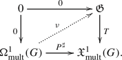
• (3) Moreover, the weak Lie 2-algebra morphism in (45) becomes the coadjoint action $({{\,\textrm{ad}\,}}_0^*,{{\,\textrm{ad}\,}}^*_1,{{\,\textrm{ad}\,}}^*_2)$ of the weak Lie 2-algebra ${\mathfrak {L}}=({\vartheta }\xrightarrow {d} {\mathfrak {g}})$ on its dual ${\mathfrak {L}}^*=({\mathfrak {g}}^*\xrightarrow {d^T}{\vartheta }^*)$:

  

  where $\nu :\wedge ^2{\mathfrak {g}}\rightarrow {{\,\textrm{Hom}\,}}({\vartheta }^*,{\mathfrak {g}}^*)$ is given by

  $$\begin{aligned} \nu (x,y)=-[x,y,~\cdot ~]_3^*,\qquad \forall x,y\in {\mathfrak {g}}. \end{aligned}$$

  This could be seen as a weak Lie 2-algebra analogue of Diagram (31).

5 Infinitesimal Multiplicative (IM) Forms on a Quasi-Lie Bialgebroid

Quasi-Lie bialgebroids serve as the infinitesimal counterparts of quasi-Poisson groupoids, while IM forms of a Lie algebroid correspond to the infinitesimal counterparts of multiplicative forms on a Lie groupoid. Given this parallelism, a natural extension of our Theorems 3.1 and 3.3 from a quasi-Poisson groupoid to a quasi-Lie bialgebroid setting is warranted. This section of the paper aims to accomplish this transition.

5.1 IM forms of a Lie algebroid

First, recall from [6] that an IM k-form of a Lie algebroid A is a pair $(\nu ,\theta )$, where $\nu : A\rightarrow \wedge ^k T^*M$ and $\theta : A\rightarrow \wedge ^{k-1}T^*M$ are bundle maps satisfying the constraints

$$\begin{aligned} \iota _{\rho (x)}\theta (y)= & {} -\iota _{\rho (y)}\theta (x),\\ \theta ([x,y])= & {} L_{\rho (x)} \theta (y)-\iota _{\rho (y)}d \theta (x)-\iota _{\rho (y)}\nu (x),\\ \text{ and } ~ \nu ([x,y])= & {} L_{\rho (x)} \nu (y)-\iota _{\rho (y)}d \nu (x), \end{aligned}$$

for $x,y\in \Gamma (A)$. In particular, an IM 1-form is a pair $(\nu ,\theta )$ where $\nu :A\rightarrow T ^*M$ is a morphism of vector bundles, $\theta \in \Gamma (A^*)$, and the following conditions are satisfied:

$$\begin{aligned} \theta [x,y]= & {} \rho (x)\theta (y)-\rho (y)\theta (x)-\langle \rho (y),\nu (x)\rangle , \end{aligned}$$

(46)

$$\begin{aligned} \nu [x,y]= & {} L_{\rho (x)} \nu (y)-\iota _{\rho (y)} d\nu (x). \end{aligned}$$

(47)

Equation (46) is also formulated as $(d_A \theta )(x,y)=\langle \rho (y),\nu (x)\rangle$ where $d_A: \Gamma (A^*)\rightarrow \Gamma (\wedge ^2 A^*)$ is the differential associated with the Lie algebroid structure of A.

Let ${\mathcal {G}}$ be a Lie groupoid over M and A the Lie algebroid of it. We need a basic map $\sigma :~\Omega ^k_{{{\,\textrm{mult}\,}}}({\mathcal {G}})\rightarrow \textrm{IM}^k(A)$ (the space of IM k-forms) for all integers k introduced in [6]—For any $\Theta \in \Omega ^k_{{{\,\textrm{mult}\,}}}({\mathcal {G}})$, define the corresponding IM k-form $\sigma (\Theta )$, say the pair $(\nu ,\theta )$, by the following relations

$$\begin{aligned} \langle \nu (x),U_1\wedge \cdots \wedge U_k\rangle= & {} d\Theta (x,U_1,\cdots ,U_k), \end{aligned}$$

(48)

$$\begin{aligned} \text{ and } \quad \langle \theta (x),U_1\wedge \cdots \wedge U_{k-1}\rangle= & {} \Theta (x,U_1,\cdots ,U_{k-1}), \end{aligned}$$

(49)

for $x\in { \Gamma } (A)$ and $U_i\in {\mathfrak {X}}^1(M)$. The multiplicativity property of $\Theta$ ensures that $(\nu ,\theta )$ fulfills the aforementioned conditions of an IM k-form of A. If ${\mathcal {G}}$ is source-simply-connected, then $\sigma$ is a one-one correspondence, and hence an isomorphism $\Omega ^k_{{{\,\textrm{mult}\,}}}({\mathcal {G}})\cong \textrm{IM}^k(A)$ of ${\mathbb {R}}$-vector spaces.

5.2 The weak graded Lie 2-algebra of IM forms on a quasi-Lie bialgebroid

If we are given a quasi-Poisson groupoid $({\mathcal {G}},P,\Phi )$, then by Theorem 3.3, we have a weak graded Lie 2-algebra $\Omega ^\bullet (M)\xrightarrow {J}\Omega ^\bullet _{{{\,\textrm{mult}\,}}}({\mathcal {G}})$. Further, if ${\mathcal {G}}$ is source-simply-connected, then by identifying $\Omega ^\bullet _{{{\,\textrm{mult}\,}}}({\mathcal {G}})$ with $\textrm{IM}^\bullet (A)$ via $\sigma$, we also have a weak graded Lie 2-algebra $\Omega ^\bullet (M)\xrightarrow {j} \textrm{IM}^\bullet (A)$.

Since quasi-Lie bialgebroids are infinitesimal replacements of quasi-Poisson groupoids [17], it is natural to expect that a weak graded Lie 2-algebra $\Omega ^\bullet (M)\xrightarrow {j} \textrm{IM}^\bullet (A)$ is directly associated with a quasi-Lie bialgebroid $(A,d_*,\Phi )$. In what follows, we demonstrate this fact. Although our statements are about the graded space of all degree IM forms $\textrm{IM}^\bullet (A)$ of a quasi-Lie bialgebroid A, for brevity most of the proofs are limited only to IM 1-forms.

We start with recalling the definitions of k-differentials and quasi-Lie bialgebroids.

A k-differential on a Lie algebroid A is a pair of linear maps $\delta :\Gamma (A)\rightarrow \Gamma (\wedge ^k A)$ and $\delta :C^\infty (M)\rightarrow \Gamma (\wedge ^{k-1} A)$ such that

$$\begin{aligned}{} & {} \delta (ff')=f\delta (f')+f'\delta (f),\quad \delta (fx)=f\delta (x)+\delta (f)\wedge x,\\{} & {} \quad \delta [x,y]=[\delta (x),y]+[x,\delta (y)], \end{aligned}$$

for $f,f'\in C^\infty (M)$ and $x,y\in \Gamma (A)$. A k-differential extends naturally to an operator $\Gamma (\wedge ^\bullet A)\rightarrow \Gamma (\wedge ^{\bullet +k-1}A)$.

Denote by $\textrm{Der}^k(A)$ the space of k-differentials. Then $\textrm{Der}^\bullet (A):=~\oplus ~_k \textrm{Der}^k(A)$ with the commutator bracket is a graded Lie algebra and $\Gamma (\wedge ^\bullet A)\xrightarrow {{\mathfrak {t}}}\textrm{Der}^\bullet (A); {\mathfrak {t}}(u)=[u,~\cdot ~]$ is a strict graded Lie 2-algebra; see [17] for details.

Definition 5.1

[29] A quasi-Lie bialgebroid is a triple $(A,d_*,\Phi )$ consisting of a Lie algebroid A, a section $\Phi \in \Gamma (\wedge ^3 A)$ and a 2-differential $d_*:\Gamma (\wedge ^\bullet A )\rightarrow \Gamma (\wedge ^{\bullet +1} A )$ satisfying $d_*^2 =[\Phi ,\,{\mathop {}\limits ^{\centerdot }}\,]$ and $d_*\Phi =0$.

The operator $d_*$ in a quasi-Lie bialgebroid gives rise to an anchor map $\rho _*:A^*\rightarrow TM$ and a bracket $[\cdot ,\cdot ]_*$ on $\Gamma (A^*)$ defined as follows:

$$\begin{aligned} \rho _*(\xi )f= & {} \langle d_*f, \xi \rangle ;\\ \langle [\xi ,\xi ']_*,x\rangle= & {} \rho _*(\xi )\langle \xi ',x\rangle -\rho _*(\xi ')\langle \xi ,x\rangle -\langle d_*x,\xi \wedge \xi '\rangle , \end{aligned}$$

for all $f\in C^\infty (M), x\in \Gamma (A)$ and $\xi ,\xi '\in \Gamma (A^*)$. But note that $(A^*,[\cdot ,\cdot ]_*,\rho _*)$ does not form a Lie algebroid. For more properties of quasi-Lie bialgebroids, see [17, 29].

Let $(A,d_*,\Phi )$ be a quasi-Lie bialgebroid as defined above. We form a 2-term complex

$$\begin{aligned} \Omega ^\bullet (M)\xrightarrow {j} \textrm{IM}^\bullet (A),\qquad j(\gamma )=(-\iota _{\rho (\cdot )} d\gamma , -\iota _{\rho (\cdot )} \gamma ). \end{aligned}$$

Furthermore, we introduce the following structure maps:

• A skew-symmetric 2-bracket $[\cdot ,\cdot ]$ on $\textrm{IM}^\bullet (A)$ defined by

  $$\begin{aligned} {[}(\nu ,\theta ),(\nu ', \theta ')]= & {} \big (\nu \circ \rho _{*}^*\circ \nu '-\nu '\circ \rho _{*}^*\circ \nu +L_{(\rho _{*} \theta )}\nu '(\cdot )-\nu '(L_\theta (\cdot ))\nonumber \\{} & {} -L_{(\rho _{*} \theta ')} \nu (\cdot )+\nu (L_{\theta '}(\cdot )),[\theta ,\theta ']_{*}\big ), \end{aligned}$$

  (50)

  for all $(\nu ,\theta )\in \textrm{IM}^p(A)$ and $(\nu ',\theta ')\in \textrm{IM}^q (A)$. Here $\rho _*^*:\Gamma (\wedge ^q T^*M)\rightarrow \Gamma (A\otimes \wedge ^{q-1}T^*M)$ is given by

  $$\begin{aligned} \rho _*^*(\gamma _1\wedge \cdots \wedge \gamma _q)=\sum _{i=1}^q(-1)^{i-1}\rho _*^*(\gamma _i)\otimes \gamma _1\wedge \cdots \widehat{\gamma _i}\wedge \cdots \wedge \gamma _q, \end{aligned}$$

  the two Lie derivatives are the Lie derivatives of $\Gamma (TM)$ on forms and of $\Gamma (A^*)$ on $\Gamma (A)$, and the bracket $[\theta ,\theta ']_*\in {{\,\textrm{Hom}\,}}(A, \wedge ^{p+q-2}T^*M)$ is given by $[\theta ,\theta ']_*=[\xi ,\xi ']_*\otimes \gamma \wedge \gamma$ for $\theta =\xi \otimes \gamma \in \Gamma (A^*\otimes \wedge ^{p-1} T^*M)$ and $\theta '=\xi '\otimes \gamma '\in \Gamma (A^*\otimes \wedge ^{q-1} T^*M)$.

• An action map $\triangleright : \textrm{IM}^p(A)\otimes \Omega ^q(M)\rightarrow \Omega ^{p+q-1}(M)$ defined by

  $$\begin{aligned} (\nu ,\theta )\triangleright \gamma =\nu (\rho _{*}^*\gamma )+L_{(\rho _* \theta )} \gamma . \end{aligned}$$

• A homotopy map (3-bracket) $[\cdot ,\cdot ,\cdot ]:\textrm{IM}^p(A)\wedge \textrm{IM}^q(A)\wedge \textrm{IM}^s(A)\rightarrow \Omega ^{p+q+s-2}(M)$ defined by

  $$\begin{aligned} {[}(\nu _1,\theta _1),(\nu _2,\theta _2),(\nu _3,\theta _3)]=d\iota _{(\iota _{(\iota _\Phi \theta _1)} \theta _2)} \theta _3+\nu _1(\iota _{\iota _\Phi \theta _2} \theta _3)+\nu _2(\iota _{\iota _\Phi \theta _3} \theta _1)+\nu _3(\iota _{\iota _\Phi \theta _1} \theta _2). \end{aligned}$$

  Here the contraction $\iota _{\cdot }$ is defined in the same fashion as in (27).

Theorem 5.2

The triple $\Omega ^\bullet (M)\xrightarrow {j} \textrm{IM}^\bullet (A)$ together with the bracket, the action, and the homotopy maps as above composes a weak graded Lie 2-algebra.

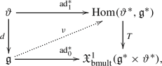
Proposition 5.3

Under the same assumptions as in the above theorem, there exists a weak graded Lie 2-algebra morphism $(\psi _0,\wedge ^{\bullet }\rho _*^*,\psi _2)$:

where

$$\begin{aligned} \psi _0(\nu ,\theta )=(\wedge ^k\rho _{*}^*)(\nu (\cdot )+d\iota _\theta (\cdot ))+(\textrm{id}\otimes (\wedge ^{k-1}\rho _{*}^*))(\iota _\theta d_*(\cdot )) \end{aligned}$$

(51)

and $\psi _2: \textrm{IM}^p(A)\wedge \textrm{IM}^q(A)\rightarrow \Gamma (\wedge ^{p+q-1}A)$ is given by

$$\begin{aligned} \psi _2((\nu ,\theta ),(\nu ',\theta '))=(\textrm{id}\otimes (\wedge ^{p+q-2} \rho _*^*))(\iota _{\iota _{\Phi } \theta } \theta '). \end{aligned}$$

The proofs of these two statements are quite involved. To save pages, in what follows we only show the $\bullet =1$ case and divide the proof into several parts. The general situation can be approached in a similar manner.

5.2.1 Well-definedness of the 2-bracket

We verify that the resulting pair $({\tilde{\nu }},{\tilde{\theta }}):=[(\nu ,\theta ),(\nu ', \theta ')]$ given by Eq. (50) is an element of $\textrm{IM}^1(A)$, namely, the pair satisfies (46) and (47).

Since $(A,d_*,\Phi )$ is a quasi-Lie bialgebroid, we have

$$\begin{aligned} d_A [\theta ,\theta ']_*=[d_A\theta ,\theta ']_*+[\theta ,d_A \theta ']_*,\qquad \forall \theta ,\theta '\in \Gamma (A^*). \end{aligned}$$

Then using (46) for $(\nu ,\theta ), (\nu ',\theta ')$ and the following relations due to [26]:

$$\begin{aligned} L_{\rho ^*_*\gamma } \theta =-[\rho ^*\gamma ,\theta ]_*-\rho ^*(\iota _{\rho _*\theta } d\gamma ),\quad \qquad L_{\rho ^*\gamma } x=-[\rho _*^*\gamma ,x]-\rho _*^*(\iota _{\rho x} d\gamma ) \end{aligned}$$

(52)

for all $\gamma \in \Omega ^1(M),\theta \in \Gamma (A^*), x\in \Gamma (A)$, we further obtain

$$\begin{aligned} d_A [\theta ,\theta ']_*(x,y)= & {} -\rho _*(\theta ')d_A \theta (x,y)+d_A \theta (L_{\theta '}x,y)+d_A \theta (x,L_{\theta '}y)-c.p.\\= & {} -\rho _*(\theta ')\langle \rho (y),\nu (x)\rangle +\langle \rho (y),\nu (L_{\theta '} x)\rangle +\langle \rho (L_{\theta '} y),\nu (x)\rangle -c.p.\\= & {} \langle y,[\rho ^*\nu (x),\theta ']_*\rangle +\langle \rho (y),\nu (L_{\theta '} x)\rangle -c.p.\\= & {} \langle y, -L_{\rho _*^* \nu (x)} \theta '-\rho ^*(\iota _{\rho _*\theta '} d\nu (x))\rangle +\langle \rho (y),\nu (L_{\theta '} x)\rangle -c.p.\\= & {} \langle y, -\rho ^*\nu '(\rho _*^* \nu (x))-\rho ^*L_{\rho _*\theta '} \nu (x)\rangle +\langle \rho y,\nu (L_{\theta '} x)\rangle -c.p.\\= & {} \langle \rho y,-\nu '\rho _*^*\nu (x)-L_{\rho _*\theta '}\nu (x)+\nu (L_{\theta '} x)+\nu \rho _*^*\nu '(x)\\{} & {} +L_{\rho _*\theta }\nu '(x)-\nu '(L_{\theta } x)\rangle . \end{aligned}$$

So we proved (46). Then it is left to check (47) for $({\tilde{\nu }},{\tilde{\theta }})$. Using the following formula:

$$\begin{aligned} L_{\theta }[x,y]=[L_{\theta }x,y]+[x,L_{\theta } y]-L_{\iota _x d_{A} \theta } y+\iota _{\iota _y d_{A} \theta } d_* x, \end{aligned}$$

(53)

we have

$$\begin{aligned} {\tilde{\nu }}[x,y]= & {} \nu \rho _*^*\nu '[x,y]+L_{\rho _*\theta }\nu '[x,y]-\nu '(L_{\theta }[x,y])-c.p.\\= & {} \nu \rho _*^*\big (L_{\rho x} \nu '(y)-\iota _{\rho y}d\nu '(x)\big )+L_{\rho _*\theta } (L_{\rho x} \nu '(y)-\iota _{\rho y} d\nu '(x))\\{} & {} -L_{\rho (L_{\theta } x)} \nu '(y)+\iota _{\rho y} d\nu '(L_{\theta } x)-L_{\rho x} \nu '(L_{\theta } y)+\iota _{\rho (L_{\theta } y)} d\nu '(x)\\{} & {} +\nu '(L_{\iota _x d_{A} \theta } y-\iota _{\iota _y d_{A} \theta } d_*x)-c.p., \end{aligned}$$

and

$$\begin{aligned}{} & {} L_{\rho x} {\tilde{\nu }}(y)-\iota _{\rho y} d{\tilde{\nu }}(x)\\{} & {} \quad =L_{\rho x}\big (\nu \rho _*^*\nu '(y)+L_{\rho _*\theta } \nu '(y)-\nu '(L_{\theta } y)\big )-\iota _{\rho y} d\big (\nu \rho _*^*\nu '(x)\\{} & {} \quad \quad +L_{\rho _*\theta } \nu '(x)-\nu '(L_{\theta } x)\big )-c.p.. \end{aligned}$$

According to Eqs. (47) and (52), we have

$$\begin{aligned} \nu \rho _*^*L_{\rho x} \nu '(y)= & {} \nu \big (\rho _*^*\iota _{\rho x} d\nu '(y)+\rho _*^*d\iota _{\rho x} \nu '(y)\big ) \\ {}= & {} \nu ([x,\rho _*^*\nu '(y)]-L_{\rho ^*\nu '(y)} x+d_{*}\iota _x \rho ^*\nu '(y))\\ {}= & {} L_{\rho x} \nu \rho _*^*\nu '(y)-\iota _{\rho \rho _*^*\nu '(y)} d\nu (x)-\nu (\iota _{\rho ^*\nu '(y)} d_* x), \end{aligned}$$

and

$$\begin{aligned} -\nu \rho _*^*\iota _{\rho y}d\nu '(x)= & {} \nu (L_{\rho ^*\nu '(x)} y+[\rho _*^*\nu '(x),y])\\= & {} \nu (L_{\rho ^*\nu '(x)} y)+L_{\rho \rho _*^* \nu '(x)} \nu (y)-\iota _{\rho y} d\nu (\rho _*^*\nu '(x)). \end{aligned}$$

Utilizing the above relations to ${\tilde{\nu }}[x,y]$, we obtain

$$\begin{aligned} {\tilde{\nu }}[x,y]-L_{\rho x} {\tilde{\nu }}(y)-\iota _{\rho y} d{\tilde{\nu }}(x)= & {} \big (L_{[\rho _* \theta ,\rho x]} \nu '(y)-L_{\rho (L_{\theta } x)} \nu '(y)\big )\\{} & {} +\big (\iota _{[\rho y,\rho _*\theta ]} d\nu '(x)+\iota _{\rho (L_{\theta } y)} d\nu '(x)\big )\\{} & {} +L_{\rho \rho _*^* \nu '(x)} \nu (y)-\iota _{\rho \rho _*^*\nu '(y)} d\nu (x)-c.p.\\= & {} 0, \end{aligned}$$

where we have used (46), the Cartan formulas

$$\begin{aligned} d\circ L_u=L_u\circ d,\qquad L_u\circ \iota _v-\iota _v \circ L_u=\iota _{[u,v]},\qquad \forall u,v\in {\mathfrak {X}}^1(M), \end{aligned}$$

and the equations

$$\begin{aligned} {[}\rho _*\theta ,\rho x]=\rho (L_{\theta } x)-\rho _*(\iota _x d_{A} \theta ),\qquad \rho _*\circ \rho ^*=-\rho \circ \rho _*^*. \end{aligned}$$

(54)

Hence we proved that $({\tilde{\nu }},{\tilde{\theta }})$ satisfies (47), and verified that $[(\nu ,\theta ),(\nu ',\theta ')]\in \textrm{IM}^1(A)$.

5.2.2 Compatibility of the 2-bracket and the action

Lemma 5.4

For any $(\nu ,\theta )\in \textrm{IM}^1(A)$ and $\gamma \in \Omega ^1(M)$, we have

$$\begin{aligned}{}[(\nu ,\theta ),j\gamma ]=j((\nu ,\theta )\triangleright \gamma ). \end{aligned}$$

Proof

Denote by $\mu \in \Omega ^1(M)$ the result of $(\nu ,\theta )\triangleright \gamma$ ($=\nu (\rho _*^*\gamma )+L_{\rho _*\theta } \gamma$). According to the definition of j, what the lemma claims is the following identity

$$\begin{aligned} {[}(\nu ,\theta ),(\iota _{\rho (\cdot )} d\gamma ,\rho ^*\gamma )]=(\iota _{\rho (\cdot )}d\mu ,\rho ^*\mu ). \end{aligned}$$

(55)

Now we prove this equality. To simplify notations, we denote by $({\hat{\nu }},{\hat{\theta }}):=[(\nu ,\theta ),(\iota _{\rho (\cdot )} d\gamma ,\rho ^*\gamma )]$ the result of left hand side. Then by Eqs. (52) and (46), we have

$$\begin{aligned} {\hat{\theta }}= & {} [\theta ,\rho ^*\gamma ]_*=L_{\rho _*^*\gamma }\theta +\rho ^*(\iota _{\rho _*\theta }d\gamma )=\iota _{\rho _*^*\gamma } d_A \theta +d_A \langle \gamma , \rho _* \theta \rangle \\{} & {} +\rho ^*(\iota _{\rho _*\theta }d\gamma )=\rho ^*\nu (\rho _*^*\gamma )+\rho ^*L_{\rho _*\theta } \gamma , \end{aligned}$$

which is exactly $\rho ^*\mu$.

We then compute ${\hat{\nu }}$. Indeed, using (52), (54), (46), (47), we can explicitly describe the value of ${\hat{\nu }}$ when it is applied to $x\in \Gamma (A)$:

$$\begin{aligned} {\hat{\nu }}(x)= & {} \nu \rho _*^*\iota _{\rho (x)} d\gamma -\iota _{\rho (\rho _*^*\nu (x))}d\gamma +L_{\rho _* \theta } \iota _{\rho x}d\gamma -\iota _{\rho (L_{\theta } x)}d\gamma \\{} & {} -L_{\rho _*\rho ^*\gamma } \nu (x)+\nu (L_{\rho ^*\gamma } x)\\= & {} \nu ([x,\rho _*^*\gamma ])-\iota _{[\rho _* \theta ,\rho x]}d\gamma +L_{\rho _* \theta } \iota _{\rho x}d\gamma -L_{\rho _*\rho ^*\gamma } \nu (x) \\= & {} \iota _{\rho x} d\nu (\rho _*^*\gamma )+\iota _{\rho x}L_{\rho _* \theta } d\gamma =\iota _{\rho x} d\mu , \end{aligned}$$

where in the second-to-last calculation, we utilized $d\circ L_{\rho _*\theta }=L_{\rho _*\theta }\circ d$. Thus we proved (55). $\quad \square$

5.2.3 Proof of Theorem 5.2

Based on the previous two subsections, it remains to show the following facts to finish the proof of Theorem 5.2.

(1). We first prove the property:

$$\begin{aligned} (j\gamma )\triangleright \gamma '=-(j\gamma ')\triangleright \gamma , \end{aligned}$$

for all $\gamma ,\gamma '\in \Omega ^1(M)$.

In fact, we can consider the map $\pi ^\sharp :=\rho \circ \rho ^*_*: T^*M\rightarrow TM$. Since $\rho \circ \rho _*^*=-\rho _*\circ \rho ^*$, $\pi ^\sharp$ gives rise to a bivector field $\pi$ on the base manifold M and thus defines a skew-symmetric bracket (not necessarily Lie) $[\cdot ,\cdot ]^{\pi }$ on $\Omega ^1(M)$. It follows that

$$\begin{aligned} (j\gamma )\triangleright \gamma '=L_{\pi ^\sharp \gamma } \gamma '-\iota _{\pi ^\sharp \gamma '} d\gamma =[\gamma ,\gamma ']^{\pi }=-(j\gamma ')\triangleright \gamma . \end{aligned}$$

(2). Next, we show that the 2-bracket (50) satisfies a generalized type of Jacobi identity:

$$\begin{aligned} {[}[(\nu _1,\theta _1),(\nu _2,\theta _2)],(\nu _3,\theta _3)]+c.p.=-j[(\nu _1,\theta _1),(\nu _2,\theta _2),(\nu _3,\theta _3)]. \end{aligned}$$

(56)

To verify the identity proposed above that involves the 2-bracket $[\cdot ,\cdot ]$, which is ${\mathbb {R}}$-bilinear, all possible combinations of $\nu _i$ and $\theta _i$ should be considered—

• (2.1) When focusing solely on the pure entries of $\nu _i$, it is easy to see that they do not contribute to the left hand side of Eq. (56). This is due to the fact that by definition, we have $[[\nu _1,\nu _2],\nu _3]+c.p.=0$.

• (2.2) Using the axioms of a quasi-Lie bialgebroid $(A, d_*, \Phi )$ ([29]) and Eq. (46), we can establish the following equality by considering only $\theta _i$ in the entries:

  $$\begin{aligned} {[}[\theta _1,\theta _2],\theta _3]+c.p.= & {} d_A\Phi (\theta _1,\theta _2,\theta _3)+\Phi (d_A \theta _1,\theta _2,\theta _3)\\{} & {} -\Phi ( \theta _1,d_A \theta _2,\theta _3)+\Phi (\theta _1,\theta _2,d_A \theta _3) \\= & {} \rho ^*d\Phi (\theta _1,\theta _2,\theta _3)+\rho ^*\nu _1(\Phi (\theta _2,\theta _3))\\{} & {} +\rho ^*\nu _2(\Phi (\theta _3,\theta _1))+\rho ^*\nu _3(\Phi (\theta _1,\theta _2))\\= & {} \rho ^*[(\nu _1,\theta _2),(\nu _2,\theta _2),(\nu _3,\theta _3)]. \end{aligned}$$

• (2.3) We have the following mixed terms:

  $$\begin{aligned}{} & {} {[}[\nu _1,\nu _2],\theta _3]+[[\nu _2,\theta _3],\nu _1]+[[\theta _3,\nu _1],\nu _2]\\{} & {} \quad = [\nu _1,\nu _2](L_{\theta _3} (\cdot ))-L_{\rho _*\theta _3}[\nu _1,\nu _2](\cdot )\\{} & {} \quad \quad +\big ( [\nu _2,\theta _3]\rho _*^*\nu _1-\nu _1\rho _*^*[\nu _2,\theta _3]-c.p.(\nu _1,\nu _2)\big )\\{} & {} \quad = (\nu _1\rho _*^*\nu _2-\nu _2\rho _*^*\nu _1)(L_{\theta _3} (\cdot ))-L_{\rho _*\theta _3}(\nu _1\rho _*^*\nu _2-\nu _2\rho _*^*\nu _1)\\{} & {} \quad \quad +\big ( \nu _2(L_{\theta _3} \rho _*^* \nu _1(\cdot ))-L_{\rho _*\theta _3}(\nu _2\rho _*^*\nu _1(\cdot ))\\{} & {} \quad \quad -\nu _1\rho ^*_*\nu _2(L_{\theta _3}(\cdot ))+\nu _1\rho _*^*(L_{\rho _*\theta _3} \nu _2(\cdot ))-c.p.(\nu _1,\nu _2)\big )\\{} & {} \quad = \nu _1\big (\rho _*^*(L_{\rho _*\theta _3} \nu _2(\cdot ))-L_{\theta _3} \rho _*^* \nu _2(\cdot )\big )-c.p.(\nu _1,\nu _2). \end{aligned}$$

• (2.4) We also have the terms

  $$\begin{aligned}{} & {} [[\nu _1,\theta _2],\theta _3]+[[\theta _3,\nu _1],\theta _2]+[[\theta _2,\theta _3],\nu _1]\\{} & {} \quad = [\nu _1,\theta _2](L_{\theta _3}(\cdot ))-L_{\rho _*\theta _3} [\nu _1,\theta _2](\cdot )-c.p.(\theta _2,\theta _3)\\{} & {} \quad \quad +L_{\rho _*[\theta _2,\theta _3]_*} \nu _1(\cdot )-\nu _1(L_{[\theta _2,\theta _3]_*} (\cdot ))\\{} & {} \quad =\nu _1(L_{\theta _2}L_{\theta _3}(\cdot ))-L_{\rho _* \theta _2} \nu _1(L_{\theta _3}(\cdot ))-L_{\rho _*\theta _3} \nu _1(L_{\theta _2}(\cdot ))\\{} & {} \quad \quad +L_{\rho _*\theta _3} L_{\rho _*\theta _2} \nu _1(\cdot )-c.p.(\theta _2,\theta _3)\\{} & {} \quad \quad +L_{\rho _*[\theta _2,\theta _3]_*} \nu _1(\cdot )-\nu _1(L_{[\theta _2,\theta _3]_*} (\cdot ))\\{} & {} \quad =\nu _1\big ([L_{\theta _2},L_{\theta _3}](\cdot )-L_{[\theta _2,\theta _3]_*}(\cdot )\big )+L_{\rho \Phi (\theta _2,\theta _3)} \nu _1(\cdot ), \end{aligned}$$

  where in the last step we used the relation

  $$\begin{aligned} \rho _*[\theta _2,\theta _3]_*=[\rho _*\theta _2,\rho _*\theta _3]+\rho \Phi (\theta _2,\theta _3). \end{aligned}$$

  (57)

  Note also that for $\alpha \in \Gamma (A^*)$ and $x\in \Gamma (A)$, by Eqs. (46) and (57), we have

  $$\begin{aligned}{} & {} \langle \rho _*^*(L_{\rho _*\theta _3} \nu _2(x))-L_{\theta _3} \rho _*^* \nu _2(x),\alpha \rangle \nonumber \\{} & {} \quad =\rho _*\theta _3\langle \nu _2(x),\rho _*\alpha \rangle -\langle \nu _2(x),[\rho _*\theta _3,\rho _*\alpha ]\rangle \nonumber \\{} & {} \quad \quad -\rho _*\theta _3\langle \nu _2(x),\rho _*\alpha \rangle +\langle \nu _2(x),\rho _*[\theta _3,\alpha ]_*\rangle \nonumber \\{} & {} \quad =\langle \nu _2(x),\rho \Phi (\theta _3,\alpha )\rangle =(d_A \theta _2)(x,\Phi (\theta _3,\alpha )), \end{aligned}$$

  (58)

  and

  $$\begin{aligned}{} & {} \langle [L_{\theta _2},L_{\theta _3}]x-L_{[\theta _2,\theta _3]_*}x,\alpha \rangle \nonumber \\{} & {} \quad =\rho _*\theta _2\langle L_{\theta _3} x,\alpha \rangle -\langle L_{\theta _3} x,[\theta _2,\alpha ]_*\rangle -c.p.(\theta _2,\theta _3)\nonumber \\{} & {} \quad \quad -\rho _*[\theta _2,\theta _3]_*\langle x,\alpha \rangle +\langle x,[[\theta _2,\theta _3]_*,\alpha ]_*\rangle \nonumber \\{} & {} \quad =\rho _*\theta _2\rho _* {\theta _3} \langle x,\alpha \rangle +\langle x,[\theta _3,[\theta _2,\alpha ]_*]_*\rangle -c.p.(\theta _2,\theta _3)\nonumber \\{} & {} \quad \quad -\rho _*[\theta _2,\theta _3]_*\langle x,\alpha \rangle +\langle x,[[\theta _2,\theta _3]_*,\alpha ]_*\rangle \nonumber \\{} & {} \quad =-\rho \Phi (\theta _2,\theta _3)\langle x,\alpha \rangle +\langle x,d_A \Phi (\theta _2,\theta _3,\alpha )+ \Phi (d_A \theta _2,\theta _3,\alpha )\nonumber \\{} & {} \quad \quad -\Phi ( \theta _2,d_A \theta _3,\alpha )+\Phi (\theta _2,\theta _3,d_A \alpha )\rangle \nonumber \\{} & {} \quad = (d_A \theta _2)(\Phi (\theta _3,\alpha ),x)-(d_A \theta _3)(\Phi (\theta _2,\alpha ),x)-\langle \alpha ,[\Phi (\theta _2,\theta _3),x]\rangle . \end{aligned}$$

  (59)

  Combining the above equalities, we find the ${{\,\textrm{Hom}\,}}(A,T^*M)$-component of the left hand side of Eq. (56):

  $$\begin{aligned}{} & {} \textrm{pr}_{{{\,\textrm{Hom}\,}}(A,T^*M)}([[(\nu _1,\theta _1),(\nu _2,\theta _2)],(\nu _3,\theta _3)]+c.p.) \\{} & {} \quad =-\nu _1([\Phi (\theta _2,\theta _3),\cdot ])+L_{\rho \Phi (\theta _2,\theta _3)} \nu _1(\cdot )+c.p.(3)\\{} & {} \quad =\iota _{\rho (\cdot )} d\nu _1(\Phi (\theta _2,\theta _3))+c.p.(3)\\{} & {} \quad =\iota _{\rho (\cdot )}d[(\nu _1,\theta _2),(\nu _2,\theta _2),(\nu _3,\theta _3)], \end{aligned}$$

  where in the second-to-last step we have used (47). Here “c.p.(3)” means the rest terms involving $\nu _2,\theta _3,\nu _3$ and $\nu _3,\theta _1,\nu _1$.

Combining the above lines, we get exactly the desired Eq. (56).

(3). Then we verify a relation:

$$\begin{aligned}{} & {} {[}(\nu _1,\theta _1),(\nu _2,\theta _2)]\triangleright \gamma -(\nu _1,\theta _1)\triangleright \big ((\nu _2,\theta _2)\triangleright \gamma \big )+(\nu _2,\theta _2)\triangleright \big ((\nu _1,\theta _1)\triangleright \gamma \big )\\{} & {} \quad =-[(\nu _1,\theta _1),(\nu _2,\theta _2),j\gamma ]. \end{aligned}$$

In fact, by (57) and (58), we can compute the left hand side of the above equation:

$$\begin{aligned}{} & {} \big (\nu _1\rho _*^*\nu _2+\nu _1(L_{\theta _2}(\cdot ))-L_{\rho _*\theta _2} \nu _1(\cdot )-c.p.(2)\big )(\rho _*^*\gamma )+L_{\rho _*[\theta _1,\theta _2]_*}\gamma \\{} & {} \quad \quad -\big (\nu _1\rho _*^*(\nu _2\rho _*^*\gamma +L_{\rho _*\theta _2}\gamma )+L_{\rho _*\theta _1}(\nu _2\rho _*^*\gamma +L_{\rho _*\theta _2}\gamma )-c.p.(2)\big )\\{} & {} \quad = \nu _1(L_{\theta _2}\rho _*^*\gamma -\rho ^*_*L_{\rho _*\theta _2} \gamma )-c.p.(2)+L_{\rho \Phi (\theta _1,\theta _2)} \gamma \\{} & {} \quad =\nu _1(\Phi (\theta _2,\rho ^*\gamma ))-\nu _2(\Phi (\theta _1,\rho ^*\gamma ))+d\Phi (\theta _1,\theta _2,\rho ^*\gamma )+\iota _{\rho \Phi (\theta _1,\theta _2)} d\gamma , \end{aligned}$$

which exactly matches with the right hand side.

(4). We finally check compatibility of the 2-bracket and the 3-bracket, namely, the relation

$$\begin{aligned}{} & {} -(\nu _4,\theta _4)\triangleright [(\nu _1,\theta _1),(\nu _2,\theta _2),(\nu _3,\theta _3)] +c.p.(4)\\{} & {} \quad =[[(\nu _1,\theta _1),(\nu _2,\theta _2)],(\nu _3,\theta _3),(\nu _4,\theta _4)] +c.p.(6). \end{aligned}$$

In fact, its left hand side reads

$$\begin{aligned}{} & {} -\nu _4\rho _*^*\big (\nu _1(\Phi (\theta _2,\theta _3))+c.p.(3)+d\Phi (\theta _1,\theta _2,\theta _3)\big )\\{} & {} \quad \quad -L_{\rho _*\theta _4}\big (\nu _1(\Phi (\theta _2,\theta _3))+c.p.(3)+d\Phi (\theta _1,\theta _2,\theta _3)\big )+c.p.(4), \end{aligned}$$

while the right hand side reads

$$\begin{aligned} \textrm{RHS}= & {} d\Phi ([\theta _1,\theta _2]_*,\theta _3,\theta _4)+\big (\nu _1\rho _*^*\nu _2+\nu _1(L_{\theta _2}(\cdot ))\\{} & {} -L_{\rho _*\theta _2}\nu _1(\cdot )-c.p.(2)\big )(\Phi (\theta _3,\theta _4))\\{} & {} +\nu _3(\Phi (\theta _4,[\theta _1,\theta _2]_*))+\nu _4(\Phi ([\theta _1,\theta _2]_*,\theta _3))+c.p.(6). \end{aligned}$$

So, subtraction of the two sides equals

$$\begin{aligned}{} & {} -\nu _4(d_*\Phi (\theta _1,\theta _2,\theta _3))+c.p.(4)\\{} & {} \quad \quad -\big (\nu _1(L_{\theta _2}\Phi (\theta _3,\theta _4))-\nu _2(L_{\theta _1}\Phi (\theta _3,\theta _4))+\nu _3(\Phi (\theta _4,[\theta _1,\theta _2]_*))\\{} & {} \quad \quad +\nu _4(\Phi ([\theta _1,\theta _2]_*,\theta _3))+c.p.(6)\big )\\{} & {} \quad \quad -\big (d(\rho _*\theta _4)(\Phi (\theta _1,\theta _2,\theta _3))+c.p.(4)+(d\Phi ([\theta _1,\theta _2]_*,\theta _3,\theta _4)+c.p.(6))\big )\\{} & {} \quad =\nu _4((d_*\Phi )(\theta _1,\theta _2,\theta _3,\cdot ))+c.p.(4)+d((d_*\Phi )(\theta _1,\theta _2,\theta _3,\theta _4)), \end{aligned}$$

which vanishes as $d_*\Phi =0$.

This completes the proof of $\Omega ^1(M)\xrightarrow {j}\textrm{IM}^1(A)$ being a weak Lie 2-algebra.

5.2.4 Proof of Proposition 5.3

(1). We first verify that $\psi _0(\nu ,\theta )\in \textrm{Der}^1(A)$, which amounts to check the following two conditions:

$$\begin{aligned}&\displaystyle \psi _0(\nu ,\theta )(fx)=f\psi _0(\nu ,\theta )(x)+\psi _0(\nu ,\theta )(f) x,\\&\displaystyle \text{ and } \psi _0(\nu ,\theta )[x,y]=[\psi _0(\nu ,\theta )(x),y]+[x,\psi _0(\nu ,\theta )(y)], \end{aligned}$$

for all $f\in C^\infty (M)$ and $x,y\in \Gamma (A)$. The proof is simple and direct—Note that $\psi _0(\nu ,\theta )=\rho _*^*\nu (\cdot )+L_\theta ^{A^*}(\cdot )$, and hence we can check the first one:

$$\begin{aligned} \psi _0(\nu ,\theta )(fx)= & {} \rho _*^*\nu (fx)+L_{\theta } (fx)=f\rho _*^*\nu (x)+fL_{\theta } (x)+\rho _*(\theta )(f)x\\= & {} f\psi _0(\nu ,\theta )(x)+\rho _*(\theta )(f)x; \end{aligned}$$

For the second one, we use (46), (47), (52) and (53), and obtain

$$\begin{aligned}{} & {} \psi _0(\nu ,\theta )[x,y]\\{} & {} \quad =\rho _*^*\nu [x,y]+L_\theta [x,y]\\{} & {} \quad =d_* \langle \rho x,\nu (y)\rangle +\rho _*^*(\iota _{\rho x} d\nu (y)-\iota _{\rho y} d\nu (x))\\{} & {} \quad \quad +[L_\theta x,y]+[x,L_\theta y]-L_{\rho ^*\nu (x)} y+\iota _{\rho ^*\nu (y)} d_*x\\{} & {} \quad =[\rho _*^*\nu (x)+L_\theta x,y]+[x,\rho _*^*\nu (y)+L_\theta y]\\{} & {} \quad =[\psi _0(\nu ,\theta )(x),y]+[x,\psi _0(\nu ,\theta )(y)]. \end{aligned}$$

(2). Next, following Eq. (52), we have

$$\begin{aligned} \psi _0(j\gamma )(x)=-\rho _*^* \iota _{\rho x} d\gamma -L_{\rho ^*\gamma } x=[\rho _*^*\gamma ,x]={\mathfrak {t}}(\rho _*^* \gamma )(x). \end{aligned}$$

This confirms that the diagram stated in the proposition is commutative.

(3). Then we check the relations

$$\begin{aligned} \psi _0[(\nu ,\theta ),(\nu ',\theta ')]-[\psi _0(\nu ,\theta ),\psi _0(\nu ',\theta ')]= & {} {\mathfrak {t}}\psi _2((\nu ,\theta ),(\nu ',\theta ')), \end{aligned}$$

(60)

$$\begin{aligned} \rho _*^*((\nu ,\theta )\triangleright \gamma )-\psi _0(\nu ,\theta )(\rho ^*_*\gamma )= & {} \psi _2((\nu ,\theta ),j\gamma ). \end{aligned}$$

(61)

In fact, by direct calculation, we have

$$\begin{aligned} \psi _0[\nu ,\nu ']-[\psi _0(\nu ),\psi _0(\nu ')]= & {} \rho _*^*\big (\nu \circ \rho _{*}^*\circ \nu '-\nu '\circ \rho _{*}^*\circ \nu )-[\rho _*^*\nu ,\rho _*^*\nu ']=0,\\ \psi _0[\theta ,\theta ']-[\psi _0(\theta ),\psi _0(\theta ')]= & {} L_{[\theta ,\theta ']_*}(\cdot )-[L_\theta (\cdot ),L_{\theta '}(\cdot )],\\ \text{ and } \psi _0[\nu ,\theta ']-[\psi _0(\nu ),\psi _0(\theta ')]= & {} \rho ^*_*(-L_{\rho _{*} \theta '} \nu (\cdot )+\nu (L_{\theta '}(\cdot )))-[\rho _*^*\nu (\cdot ),L_{\theta '}(\cdot )]\\= & {} -\rho ^*_*L_{\rho _{*} \theta '} \nu (\cdot )+L_{\theta '} \rho _*^*\nu (\cdot ). \end{aligned}$$

Using these relations together, (58), and (59), we can check (60):

$$\begin{aligned} \psi _0[(\nu ,\theta ),(\nu ',\theta ')]-[\psi _0(\nu ,\theta ),\psi _0(\nu ',\theta ')]= & {} [\Phi (\theta ,\theta '),\cdot ]={\mathfrak {t}}\psi _2((\nu ,\theta ),(\nu ',\theta ')). \end{aligned}$$

To examine (61), we have

$$\begin{aligned} \rho _*^*((\nu ,\theta )\triangleright \gamma )-\psi _0(\nu ,\theta )(\rho _*^*\gamma )= & {} \rho _*^*(\nu (\rho _*^*\gamma )+L_{\rho _*\theta } \gamma )-\rho _*^*\nu (\rho _*^*\gamma )-L_{\theta } (\rho _*^*\gamma )\\= & {} \psi _2((\nu ,\theta ),j\gamma ), \end{aligned}$$

where we have used (58) again.

(4). Finally, we prove

$$\begin{aligned} \rho _*^*[(\nu _1,\theta _1),(\nu _2,\theta _2),(\nu _3,\theta _3)]= & {} \psi _0(\nu _1,\theta _1)\triangleright \psi _2((\nu _2,\theta _2),(\nu _3,\theta _3))\\{} & {} -\psi _2([(\nu _1,\theta _1),(\nu _2,\theta _2)],(\nu _3,\theta _3))+c.p. \end{aligned}$$

Let us compare the two sides of this equation. By definition and (46), we have

$$\begin{aligned} \textrm{LHS}= & {} \rho ^*_*\nu _1(\Phi (\theta _2,\theta _3))+c.p.+d_*(\Phi (\theta _1,\theta _2,\theta _3)),\\ \textrm{RHS}= & {} \rho _*^*\nu _1(\Phi (\theta _2,\theta _3))+L_{\theta _1}\Phi (\theta _2,\theta _3)-\Phi ([\theta _1,\theta _2]_*,\theta _3)+c.p. \end{aligned}$$

Since $d_*\Phi =0$, it is easy to see that they are identical. This completes the proof of $(\psi _0,\rho _*^*,\psi _2)$ being a weak Lie 2-algebra morphism.

5.2.5 More corollaries

Recall that a Lie bialgebroid is a special quasi-Lie algebroid $(A,d_*, \Phi )$ where $\Phi$ is trivial [26]. So, let us use the pair $(A,d_*)$ to denote a Lie bialgebroid. The following corollary directly follows from Theorem 5.2 and Proposition 5.3.

Corollary 5.5

Let $(A,d_*)$ be a Lie bialgebroid over the base manifold M.

• (i) The triple $\Omega ^\bullet (M)\xrightarrow {j} \textrm{IM}^\bullet (A)$ together with the bracket and action map as earlier constitutes a strict graded Lie 2-algebra.

• (ii) There is a strict graded Lie 2-algebra homomorphism $(\psi _0,\rho _*^*)$:

  

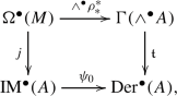
  where $\psi _0$ is given by Eq. (51).

We finally consider the particular case of quasi-Lie bialgebroids whose base manifolds are single points, i.e., quasi-Lie bialgebras. Indeed, it is easily seen that for a Lie algebra ${\mathfrak {G}}$, we have $\textrm{IM}^k({\mathfrak {G}})=0$ for all $k\geqslant 2$; and an IM 1-form of ${\mathfrak {G}}$ is simply an element $\theta \in {\mathfrak {G}}^*$ such that ${{\,\textrm{ad}\,}}_x^*\theta =0$ for all $x\in {\mathfrak {G}}$. So we can identify $\textrm{IM}^1({\mathfrak {G}})$ with $({\mathfrak {G}}^*)^{\textrm{ad}}$ (the space of $\textrm{ad}^*$-invariant elements in ${\mathfrak {G}}^*$), and thereby, Theorem 5.2 and Proposition 5.3 yield the following corollary.

Corollary 5.6

Let $({\mathfrak {G}},d_*,\Phi )$ be a quasi-Lie bialgebra.

• (i) There is a Lie algebra structure $\textrm{IM}^1({\mathfrak {G}})=({\mathfrak {G}}^*)^{\textrm{ad}}$, where the bracket is $[\cdot ,\cdot ]_*$.

• (ii) There is a weak Lie 2-algebra homomorphism $(\psi _0,0,\psi _2)$ between two strict Lie 2-algebras:

  

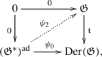
  where $\psi _0(\theta )={{\,\textrm{ad}\,}}_\theta ^*(\cdot )$ and $\psi _2:\wedge ^2 ({\mathfrak {G}}^*)^{\textrm{ad}}\rightarrow {\mathfrak {G}}$ is given by

  $$\begin{aligned} \psi _2(\theta ,\theta ')=\Phi (\theta ,\theta '). \end{aligned}$$

5.3 Relating linear forms and multivector fields on a quasi-Lie bialgebroid

Let A be a vector bundle over M. Denote by $\Omega ^k_{\textrm{lin}}(A)$ and ${\mathfrak {X}}_{\textrm{lin}}^k(A)$, respectively, the spaces of linear k-forms [6] and linear k-vector fields [17] on A. Alternatively, one can use the identifications $\Omega ^\bullet _{\textrm{lin}}(A)\cong \Gamma ({\mathfrak {J}}^\bullet A^*)$ and ${\mathfrak {X}}^\bullet _{\textrm{lin}}(A)\cong \Gamma ({\mathfrak {D}}^\bullet A^*)$ (see [22] and notations therein).

If A is equipped with a quasi-Lie bialgebroid structure $(A,d_*,\Phi )$, then the operator $d_*$ gives rise to a 2-bracket on $\Gamma (A^*)$ (but not a Lie bracket), and it corresponds to a linear bivector field $P_A\in {\mathfrak {X}}_{\textrm{lin}}^2(A)$ on A. In the same manner as that of the P-bracket in Eq. (10), this $P_A$ defines a $P_A$-bracket $[\cdot ,\cdot ]^{P_A}$ on $\Omega ^\bullet _{{{\,\textrm{lin}\,}}}(A)$. In the meantime, $P_A$ induces a map

$$\begin{aligned} \wedge ^\bullet P_A^\sharp : \Omega ^\bullet _{{{\,\textrm{lin}\,}}}(A)\rightarrow {\mathfrak {X}}^\bullet _{{{\,\textrm{lin}\,}}}(A). \end{aligned}$$

Due to [6], we have an inclusion $\iota : \textrm{IM}^\bullet (A)\hookrightarrow {}\Omega ^\bullet _{\textrm{lin}}(A)$ given by

$$\begin{aligned} \iota (\nu ,\theta )=\Lambda _\nu +d\Lambda _\theta ,\qquad (\Lambda _\mu )_x:=(dq_A)^*\nu (x), \qquad \forall x\in A, \end{aligned}$$

(62)

where $\Lambda _\theta$ is defined in the same fashion as that of $\Lambda _\nu$ and $q_A:A\rightarrow M$ is the projection. We will verify that $\textrm{IM}^\bullet (A)$ with the bracket given in (50) is a subalgebra of $(\Omega ^\bullet _{\textrm{lin}}(A),[\cdot ,\cdot ]^{P_A})$ (in Proposition 5.7, (i)).

According to [17], k-differentials of A are special instances of linear k-vector fields on A. In other words, we have an inclusion $\kappa : \textrm{Der}^k(A)\hookrightarrow {\mathfrak {X}}^k_{\textrm{lin}}(A)$ determined by

$$\begin{aligned} \kappa (\delta )(dl_{\xi _1},\cdots ,dl_{\xi _{k-1}}, dq_A^*f)= & {} q_A^* \langle \delta f, \xi _1\wedge \cdots \wedge \xi _{k-1} \rangle ; \end{aligned}$$

(63)

$$\begin{aligned} \kappa (\delta )(dl_{\xi _1},\cdots ,dl_{\xi _k} )_x= & {} \sum _{i=1}^k(-1)^{i+k}\kappa (\delta )(\cdots ,\widehat{dl_{\xi _i}},\cdots , dq_A^*\xi _i (x))\nonumber \\{} & {} -\langle \delta x, \xi _1\wedge \cdots \wedge \xi _k\rangle \end{aligned}$$

(64)

for $\xi _i \in \Gamma (A^*), x\in \Gamma (A)$ and $f\in C^\infty (M)$.

Proposition 5.7

Let $(A,d_*,\Phi )$ be a quasi-Lie bialgebroid.

• (i) We have the following commutative diagram:

  

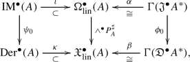
  where $\psi _0$ is given by Eq. (51) and

  $$\begin{aligned} \phi _0(\mu )(\jmath ^1\xi _1,\cdots ,\jmath ^1\xi _\bullet )=\mu ([\xi _1,\cdot ]_*,\cdots ,[\xi _\bullet ,\cdot ]_*) \end{aligned}$$

  for $\mu \in \Gamma ({\mathfrak {J}}^\bullet A^*)\subset {{\,\textrm{Hom}\,}}(\wedge ^\bullet {\mathfrak {D}}A^*,A^*)$ and $\xi _i\in \Gamma (A^*)$.

• (ii) Regarding the 2-brackets of the top objects and the natural graded Lie bracket of commutator of the bottom objects, every horizontal map preserves the relevant brackets.

Proof

(i) For simplicity, we only give the proof for $\bullet =1$. We use the equality $\psi _0(\nu ,\theta )(x)=\rho _*^*\nu (x)+L_\theta x=\rho ^*_*(\nu (x)+d\theta (x))+\iota _\theta d_*x$ (for all $x\in \Gamma (A)$), and compute the following relations:

$$\begin{aligned} \kappa (\psi _0(\nu ,\theta ))(dq_A^*f)= & {} q_A^*((\rho _*\theta )f);\\ \kappa (\psi _0(\nu ,\theta ))(dl_\xi )_x= & {} \kappa (\psi _0(\nu ,\theta ))(dq_A^*\xi (x))-\langle \rho ^*_*(\nu (x)+d\theta (x))+\iota _\theta d_*x,\xi \rangle \\= & {} \rho _*\theta (\xi (x))-\langle \nu (x)+d\theta (x),\rho _*\xi \rangle -\langle d_*x,\theta \wedge \xi \rangle \\= & {} -\langle \rho _*\xi ,\nu (x)\rangle +\langle x,[\theta ,\xi ]_*\rangle . \end{aligned}$$

Then comparing with the following lines

$$\begin{aligned} P_A^\sharp (\iota (\nu ,\theta ))(dq_A^*f)= & {} P_A((dq_A)^*\nu (\cdot )+dl_\theta ,dq_A^*f)=q_A^*((\rho _* \theta )f),\\ P_A^\sharp (\iota (\nu ,\theta ))(dl_\xi )_x= & {} P_A((dq_A)^*\nu (x)+dl_\theta ,dl_\xi )\\= & {} P_A((dq_A)^*\nu (x),dl_\xi ))+P_A(dl_\theta ,dl_\xi )_x\\= & {} -\langle \rho _*\xi ,\nu (x)\rangle +\langle x, [\theta ,\xi ]_*\rangle , \end{aligned}$$

one immediately proves $\kappa \circ \psi _0=P_A^\sharp \circ \iota$.

Given any $\jmath ^1\xi \in \Gamma ({\mathfrak {J}}^1 A^*)$, note that $\phi _0(\jmath ^1\xi )=[\xi ,\cdot ]_*$, we have

$$\begin{aligned} \langle P_A^\sharp \alpha (\jmath ^1\xi ), dl_\eta \rangle= & {} P_A(dl_\xi ,dl_\eta )=l_{[\xi ,\eta ]_*},\qquad \forall \xi ,\eta \in \Gamma (A^*),\\ \langle \beta \phi _0(\jmath ^1\xi ), dl_\eta \rangle= & {} \langle \beta ([\xi ,\cdot ]_*),dl_\eta \rangle =l_{[\xi ,\eta ]_*}, \end{aligned}$$

which clearly implies that $P_A^\sharp \circ \alpha = \beta \circ \phi _0$.

(ii) It is known from [22, Theorem 2.1] and [17, Proposition 3.8] that $\beta$ and $\kappa$ are Lie algebra isomorphisms. So we are left to show the following relations:

$$\begin{aligned} \iota [(\nu ,\theta ),(\nu ',\theta ')]= & {} [\iota (\nu ,\theta ),\iota (\nu ',\theta ')]^{P_A},\qquad \forall (\nu ,\theta ),(\nu ',\theta ')\in \textrm{IM}^1(A), \end{aligned}$$

(65)

$$\begin{aligned} \alpha ([\mu ,\mu ']_{{\mathfrak {J}}^1 A^*})= & {} [\alpha (\mu ),\alpha (\mu ')]^{P_A},\qquad \forall \mu ,\mu '\in \Gamma ({\mathfrak {J}}^1 A^*). \end{aligned}$$

(66)

Let us denote $({\tilde{\nu }},{\tilde{\theta }})=[(\nu ,\theta ),(\nu ',\theta ')]$, where, by (50), ${\tilde{\theta }}=[\theta ,\theta ']_*$. Then Eq. (65) is equivalent to

$$\begin{aligned} (\Lambda _{{\tilde{\nu }}},d\Lambda _{[\theta ,\theta ']_*})=[\Lambda _\nu +d\Lambda _\theta ,\Lambda _{\nu '}+d\Lambda _{\theta '}]^{P_A}. \end{aligned}$$

By definition, we have $\Lambda _{\theta }=l_{\theta }\in C^\infty _{lin}(A)$; then by $[dl_{\theta },dl_{\theta '}]^{P_A}=dl_{[\theta ,\theta ']_*}$, we get $d\Lambda _{[\theta ,\theta ']}=[d\Lambda _\theta ,d\Lambda _{\theta '}]^{P_A}$. Therefore, we can compute

$$\begin{aligned} {[}\Lambda _\nu ,\Lambda _{\nu '}]^{P_A}= & {} [(dq_A)^*\nu ,(dq_A)^*\nu ']^{P_A}\\= & {} dP_A((dq_A)^*\nu ,(dq_A)^*\nu ')+\big (\iota _{P_A^\sharp (dq_A)^*\nu } d(dq_A)^*\nu '-c.p.(\nu ,\nu ')\big )\\= & {} 0-(dq_A)^*(\nu '\rho _*^*\nu -\nu \rho _*^*\nu '), \end{aligned}$$

where we have used the fact that $(P_A^\sharp (dq_A)^*\nu )_x=-\rho _*^*\nu (x)\in A_{m}$ for $x\in A_m$, which is easily verified using local coordinates.

In the meantime, we find

$$\begin{aligned} {[}d\Lambda _\theta ,\Lambda _{\nu '}]^{P_A}= & {} [dl_\theta ,(dq_A)^*\nu ']^{P_A}\\= & {} L_{P_A^\sharp (dl_\theta )} (dq_A)^*\nu '\\= & {} (dq_A)^*(L_{\rho _*\theta } \nu '(\cdot )-\nu '(L_\theta (\cdot )). \end{aligned}$$

Combining these equalities, we obtain the desired (65). For (66), taking $\mu =\jmath ^1\xi$ and $\mu '=\jmath ^1\xi '$, we have

$$\begin{aligned} \alpha [\jmath ^1\xi ,\jmath ^1\xi ']_{{\mathfrak {J}}^1 A^*}=\alpha (\jmath ^1[\xi ,\xi ']_*)=dl_{[\xi ,\xi ']_*}=[dl_\xi ,dl_{\xi '}]^{P_A}=[\alpha (\jmath ^1\xi ),\alpha (\jmath ^1\xi ')]^{P_A}. \end{aligned}$$

This completes the proof. $\quad \square$

5.4 Compatibility of the two weak graded Lie 2-algebras

In this part, we connect our constructions of weak graded Lie 2-algebras, respectively, on the groupoid level and on the associate tangent Lie algebroid level.

5.4.1 The main results

We need two basic mappings.

• The correspondence $\sigma :~\Omega ^\bullet _{{{\,\textrm{mult}\,}}}({\mathcal {G}})\rightarrow \textrm{IM}^\bullet (A)$ is given as in Eqs. (48) and (49); see [6] for more details.

• The map $\tau :~{\mathfrak {X}}^\bullet _{{{\,\textrm{mult}\,}}}({\mathcal {G}})\rightarrow \textrm{Der}^\bullet (A)$ given in [17] is defined as follows—For any $\Pi \in {\mathfrak {X}}^\bullet _{{{\,\textrm{mult}\,}}}({\mathcal {G}})$, there is a unique $\tau (\Pi )\in \textrm{Der}^\bullet (A)$ subject to the relations

  $$\begin{aligned} \overrightarrow{\tau (\Pi )f}=[t^*f, \Pi ],\qquad \overrightarrow{\tau (\Pi ) x}=[\overrightarrow{x},\Pi ],\qquad \forall f\in C^\infty (M),x\in \Gamma (A). \end{aligned}$$

Proposition 5.8

Let $({\mathcal {G}},P,\Phi )$ be a quasi-Poisson Lie groupoid and $(A,d_*,\Phi )$ the corresponding quasi-Lie bialgebroid. Then the maps $P^\sharp$ and $\psi _0$ (given by Proposition 5.3) together with $\sigma$ and $\tau$ defined above form a commutative diagram:

Moreover, if ${\mathcal {G}}$ is s-connected and simply connected, then both $\sigma$ and $\tau$ are isomorphisms.

Proposition 5.9

Under the same assumption and notation as in Proposition 5.8, the triple of maps $(\sigma ,\textrm{id},0)$ is a strict morphism of weak graded Lie 2-algebras:

If ${\mathcal {G}}$ is s-connected and simply connected, then $(\sigma ,\textrm{id},0)$ is an isomorphism.

5.4.2 Proofs of the main results

Proof of Proposition 5.8

Again, we only give the proof for $\bullet =1$. Take any $\Theta \in \Omega ^1_{{{\,\textrm{mult}\,}}}({\mathcal {G}})$ and suppose that $\sigma (\Theta )=(\nu ,\theta )\in \textrm{IM}^1(A)$. The commutativity relation $\psi _0\circ \sigma =\tau \circ P^\sharp$ amounts to

$$\begin{aligned} \overrightarrow{\rho _*^*\nu (x)+L_\theta x}=[\overrightarrow{x},P^\sharp \Theta ],\qquad \forall x\in \Gamma (A). \end{aligned}$$

To prove it, we need to check

$$\begin{aligned} \rho ^*_*\nu (x)+L_\theta x=[\overrightarrow{x}, P^\sharp \Theta ]|_M. \end{aligned}$$

In fact, we have

$$\begin{aligned} (L_{\overrightarrow{x}} P)^\sharp (\Theta )= & {} L_{\overrightarrow{x}} (P^\sharp \Theta )-P^\sharp (L_{\overrightarrow{x}} \Theta )= [\overrightarrow{x},P^\sharp \Theta ]-P^\sharp (d\iota _{\overrightarrow{x}} \Theta +\iota _{\overrightarrow{x}} d\Theta ), \end{aligned}$$

and hence

$$\begin{aligned} {[}\overrightarrow{x}, P^\sharp \Theta ]|_M= & {} [\overrightarrow{x},P]^\sharp (\Theta )|_M +P^\sharp (d\iota _{\overrightarrow{x}}\Theta )+\iota _{\overrightarrow{x}} d\Theta )|_M\\= & {} \iota _\theta d_*x+\rho _*^*(d\theta (x)+\nu (x))\\= & {} \rho ^*_*\nu (x)+L_\theta x. \end{aligned}$$

$\square$

Before we proceed to the proof of Proposition 5.9, a technical lemma is needed. Recall from [12, Lemma 4.8] that for $X\in {\mathfrak {X}}^1_{{{\,\textrm{mult}\,}}}({\mathcal {G}})$ and $\Theta \in \Omega ^k_{{{\,\textrm{mult}\,}}}({\mathcal {G}})$, we have the contraction $\iota _X \Theta \in \Omega ^{k-1}_{{{\,\textrm{mult}\,}}}({\mathcal {G}})$ and the Lie derivative $L_X\Theta \in \Omega ^k_{{{\,\textrm{mult}\,}}}({\mathcal {G}})$ since the de Rham differential preserves multiplicativity properties. Now we would like to find the IM-forms corresponding to $\iota _X \Theta$ and $L_X\Theta$ via $\sigma$ defined by (48) and (49).

Lemma 5.10

For $X\in {\mathfrak {X}}^1_{{{\,\textrm{mult}\,}}}({\mathcal {G}}), \Theta \in \Omega ^k_{{{\,\textrm{mult}\,}}}({\mathcal {G}})$, suppose that $\tau (X)=(\delta _0,\delta _1)\in \textrm{Der}^1 (A)$, $\sigma (\Theta )=(\nu ,\theta )\in \textrm{IM}^k(A)$, $\sigma (\iota _X \Theta )=({\tilde{\nu }},{\tilde{\theta }})\in \textrm{IM}^{k-1}(A)$, and $\sigma (L_X \Theta )=({\hat{\nu }},{\hat{\theta }})\in \textrm{IM}^{k}(A)$. Then we have

$$\begin{aligned} {\tilde{\nu }}(x)=\iota _{\delta _0}(\nu (x))+L_{\delta _0}(\theta (x))-\theta (\delta _1 x),\qquad {\tilde{\theta }}(x)=-\iota _{\delta _0}(\theta (x)),\qquad \forall x\in \Gamma (A), \end{aligned}$$

and

$$\begin{aligned} {\hat{\nu }}(x)=L_{\delta _0} (\nu (x))-\nu (\delta _1 x),\qquad {\hat{\theta }}(x)=L_{\delta _0} (\theta (x))-\theta (\delta _1 x). \end{aligned}$$

Proof

The proof is simply straightforward computations—For $U_i\in TM$, we have

$$\begin{aligned} \langle {\tilde{\theta }}(x), U_1\wedge \cdots \wedge U_{k-2}\rangle= & {} (\iota _X \Theta )(x,U_1,\cdots , U_{k-2})\\= & {} -\Theta (x,X|_M,U_1,\cdots ,U_{k-2})\\= & {} -\langle \iota _{\delta _0} \theta (x), U_1\wedge \cdots \wedge U_{k-2}\rangle , \end{aligned}$$

and

$$\begin{aligned}{} & {} \langle {\tilde{\nu }}(x), U_1\wedge \cdots \wedge U_{k-1}\rangle \\{} & {} \quad =d(\iota _X \Theta )(x,U_1,\cdots , U_{k-1})\\{} & {} \quad =(L_X \Theta -\iota _X d\Theta )(x,U_1,\cdots ,U_{k-1})\\{} & {} \quad =X|_M\Theta (x,U_1,\cdots ,U_{k-1})-\Theta ([X,\overrightarrow{x}]|_M,U_1,\cdots ,U_k)\\{} & {} \quad \quad -\sum _i \Theta (x,\cdots ,[X|_M,U_i],\cdots )+\langle \iota _{\delta _0}\nu (x),U_1\wedge \cdots \wedge U_{k-1})\\{} & {} \quad =\langle L_{\delta _0} \theta (x)-\theta (\delta _1x)+\iota _{\delta _0}\nu (x),U_1\wedge \cdots \wedge U_{k-1}\rangle . \end{aligned}$$

These are the desired formulas of ${\tilde{\nu }}$ and ${\tilde{\theta }}$.

Based on the well-known fact that the IM k-form $\sigma (d\Theta )=(0,\nu )$ if $\sigma (\Theta )=(\nu ,\theta )\in \textrm{IM}^{k-1}(A)$, we can determine the IM k-forms of $d\iota _X \Theta$ and $\iota _X d\Theta$ as follows:

$$\begin{aligned} \sigma (d\iota _X \Theta )=(0,{\tilde{\nu }}),\qquad \sigma (\iota _X d\Theta )=\big (L_{\delta _0}(\nu (\cdot ))-\nu (\delta _1 (\cdot )), -\iota _{\delta _0}(\nu (\cdot ))\big ). \end{aligned}$$

So the IM k-form of $L_X \Theta$ is as described. $\quad \square$

Proof of Proposition 5.9

We only prove the case of $\bullet =1$. We first show that, for $\Theta$ and $\Theta '\in \Omega ^1_{{{\,\textrm{mult}\,}}}({\mathcal {G}})$ mapping to, respectively, $(\nu ,\theta ),(\nu ',\theta ')\in \textrm{IM}^1(A)$ by $\sigma$, the resulting $[\Theta ,\Theta ']_{P}\in \Omega ^1_{{{\,\textrm{mult}\,}}}({\mathcal {G}})$ is mapped to $[(\nu ,\theta ),(\nu ',\theta ')]$ (defined in (50)).

By definition, we have

$$\begin{aligned} {[}\Theta ,\Theta ']^P=L_{P^\sharp \Theta } \Theta '-\iota _{P^\sharp \Theta '} d\Theta . \end{aligned}$$

It follows from Proposition 5.8 that the 1-differential $\sigma (P^\sharp \Theta )=(\delta _0,\delta _1)\in \textrm{Der}^1(A)$ is

$$\begin{aligned} \delta _0=\rho _* \theta ,\qquad \delta _1(x)=\rho _*^*\nu (x)+L_\theta x. \end{aligned}$$

A well-known fact is the IM 2-form $\sigma (d\Theta )$ $=(0,\nu )$ provided that $\sigma (\Theta )=(\nu ,\theta )\in \textrm{IM}^1(A)$. Applying the technical Lemma 5.10, for $\iota _{P^\sharp \Theta '} d\Theta \in \Omega ^1_{{{\,\textrm{mult}\,}}}({\mathcal {G}})$, the value of $\sigma (\iota _{P^\sharp \Theta '} d\Theta )$ $=(\nu _1,\theta _1)\in \textrm{IM}^1(A)$ is given by

$$\begin{aligned} \nu _{1}(x)= & {} L_{\rho _*\theta '} \nu (x)-\nu (\rho _*^*\nu '(x)+L_{\theta '} x),\\ \theta _{1}(x)= & {} -\iota _{\rho _*\theta '} \nu (x)=-\langle \nu (x),\rho _*\theta '\rangle . \end{aligned}$$

And $\sigma (L_{P^\sharp \Theta } \Theta ')=(\nu _{2},\theta _{2})\in \textrm{IM}^1(A)$ is given by

$$\begin{aligned} \nu _{2}(x)= & {} L_{\rho _*\theta } \nu '(x)-\nu '(\rho _*^*\nu (x)+L_{\theta } x),\\ \theta _{2}(x)= & {} L_{\rho _*\theta } \theta '(x)-\theta '(\rho _*^*\nu (x)+L_{\theta } x)=-\langle \rho _* \theta ',\nu (x)\rangle +\langle [\theta ,\theta ']_*,x\rangle . \end{aligned}$$

Thus, assuming $\sigma ([\Theta ,\Theta ']^P)=({\tilde{\nu }},{\tilde{\theta }})$, we have

$$\begin{aligned} {\tilde{\nu }}(x)= & {} \nu _2(x)-\nu _1(x)=L_{\rho _*\theta } \nu '(x)-\nu '(\rho _*^*\nu (x)+L_\theta x)-L_{\rho _*\theta '} \nu (x)\\{} & {} +\nu (\rho _*^*\nu '(x)+L_{\theta '} x),\\ {\tilde{\theta }}(x)= & {} \theta _2(x)-\theta _1(x)=\langle [\theta ,\theta ']_*,x\rangle . \end{aligned}$$

Comparing with (50), we have proved

$$\begin{aligned} \sigma ([\Theta ,\Theta ']^P)=({\tilde{\nu }},{\tilde{\theta }})=[(\nu ,\theta ),(\nu ',\theta ')]. \end{aligned}$$

(67)

Then for $\gamma \in \Omega ^1(M)$, by [6, Consequence (a) of Theorem 2], we have

$$\begin{aligned} \sigma (J\gamma )=\sigma (s^*\gamma -t^*\gamma )=(-\iota _{\rho (\cdot )} d\gamma , -\rho ^*\gamma )=j(\gamma ). \end{aligned}$$

(68)

Therefore, it remains to prove that

$$\begin{aligned} {[}\Theta _1,\Theta _2,\Theta _3]^\Phi =[(\nu _1,\theta _1),(\nu _2,\theta _2),(\nu _3,\theta _3)],\qquad \forall \Theta _i\in \Omega ^1_{{{\,\textrm{mult}\,}}}({\mathcal {G}}), \end{aligned}$$

(69)

where $(\nu _i,\theta _i)=\sigma (\Theta _i)\in \textrm{IM}^1(A)$. In fact, we have

$$\begin{aligned} s^*[\Theta _1,\Theta _2,\Theta _3]^\Phi= & {} d\overleftarrow{\Phi }(\Theta _1,\Theta _2,\Theta _3)+\big (\iota _{\overleftarrow{\Phi }(\Theta _1,\Theta _2)} d\Theta _3+c.p.\big )\\= & {} s^*d\Phi (\theta _1,\theta _2,\theta _3)+s^*\big (\nu _3(\Phi (\theta _1,\theta _2))+c.p.\big )\\= & {} s^*[(\nu _1,\theta _1),(\nu _2,\theta _2),(\nu _3,\theta _3)], \end{aligned}$$

which justifies (69) (as $s^*$ is injective). In conclusion, Eqs. (67)–(69) imply that $(\sigma ,\textrm{id},0)$ is a Lie 2-algebra isomorphism. $\quad \square$

5.4.3 A summary diagram

In summary, if a quasi-Poisson groupoid $({\mathcal {G}},P,\Phi )$ is s-connected and simply connected, then regarding the associated quasi-Lie bialgebroid $(A,d_*,\Phi )$, we have the following commutative diagrams:

Here, the front and back faces are weak graded Lie 2-algebra morphisms as described by Propositions 3.2 and 5.3 (observing that $p^\sharp =\rho _*^*$), respectively.

References

Baez, J., Crans, A.: Higher dimensional algebra VI: Lie \(2\)-algebras. Theory Appl. Categ. 12, 492–538 (2014)
Baez, J., Lauda, A.: Higher-dimensional algebra V: 2-groups. Theo. Appl. Categ. 12, 423–491 (2004)
Bandiera, R., Chen, Z., Stiénon, M., Xu, P.: Shifted derived Poisson manifolds associated with Lie Pairs. Commun. Math. Phys. 375, 1717–1760 (2020)
Berwick-Evans, D., Lerman, E.: Lie \(2\)-algebras of vector fields. Pac. J. Math. 309, 1–34 (2020)
Bonechi, F., Ciccoli, N., Laurent-Gengoux, C., Xu, P.: Shifted Poisson structures on differentiable stacks. Int. Math. Res. Not. 2022(9), 6627–6704 (2022)
Bursztyn, H., Cabrera, A.: Multiplicative forms at the infinitesimal level. Math. Ann. 353, 663–705 (2012)
Bursztyn, H., Drummond, T.: Lie theory of multiplicative tensors. Math. Ann. 375, 1489–1554 (2019)
Bursztyn, H., Iglesias-Ponte, D., Severa, P.: Courant morphisms and moment maps. Math. Res. Lett. 16(2), 215–232 (2009)
Cabrera, A., Marcut, I., Salazar, M.A.: Local formulas for multiplicative forms. Transf. Groups 27(2), 371–401 (2022)
Coste, A., Dazord, P., Weinstein, A.: Groupoildes Symplectiques. Publ. Delp. Math. Nouvelle Seirie. A vol. 2, pp. 1–62. Univ. Claude Bernard, Lyon (1987)
Chen, Z., Lang, H., Liu, Z.: On the reduced space of multiplicative multi-vectors, arXiv:2003.13384
Chen, Z., Lang, H., Liu, Z.: Multiplicative forms on Poisson groupoids. Sci. China Math. (to appear)
Chen, Z., Stiénon, M., Xu, P.: Poisson \(2\)-groups. J. Differ. Geom. 94(2), 209–240 (2013)
Crainic, M., Salazar, M.A., Struchiner, I.: Multiplicative forms and Spencer operators. Math. Z. 279(3–4), 939–979 (2015)
Drinfeld, V.G.: Quantum groups. In: Proceedings of the International Congress of Mathematicians (Berkeley, CA, 1986), vol. 1, pp. 798–820. American Mathematical Society, Providence (1987)
Gualtieri, M., Matviichuk, M., Scott, G.: Deformation of Dirac structures via \(L_\infty \)-algebras. Int. Math. Res. Not. 2020(14), 4295–4323 (2020)
Iglesias-Ponte, D., Laurent-Gengoux, C., Xu, P.: Universal lifting theorem and quasi-Poisson groupoids. J. Eur. Math. Soc. 14(3), 681–731 (2012)
Kosmann-Schwarzbach, Y.: Quasi-bigebres de Lie et groupes de Lie quasi-Poisson. C. R. Acad. Sci. Paris 312, 391–394 (1991)
Kosmann-Schwarzbach, Y.: Jacobian quasi-bialgebras and quasi-Poisson Lie groups. Contemp. Math. 132, 459–489 (1992)
Kosmann-Schwarzbach, Y., Magri, F.: Poisson–Nijenhuis structures. Ann. Inst. H. Poincare Phys. Theor. 53, 35–81 (1990)
Lada, T., Stasheff, J.: Introduction to SH Lie algebras for physicists. Int. J. Theor. Phys. 32(7), 1087–1103 (1993)
Lang, H., Sheng, Y.: Linearization of the higher analogue of Courant algebroids. J. Geom. Mech. 12, 585–606 (2020)
Laurent-Gengoux, C., Stiénon, M., Xu, P.: Lectures on Poisson groupoids. Geom. Topol. Monogr. 17, 473–502 (2011)
Lu, J.-H., Weinstein, A.: Poisson Lie groups, dressing transformations, and Bruhat decompositions. J. Differ. Geom. 31, 501–526 (1990)
Mackenzie, K.: General Theory of Lie Groupoids and Lie Algebroids, London Mathematical Society Lecture Note Series, vol. 213. Cambridge University Press, Cambridge
Mackenzie, K., Xu, P.: Lie bialgebroids and Poisson groupoids. Duke Math. J. 73, 415–452 (1994)
Mikami, K., Weinstein, A.: Moments and reduction for symplectic groupoid actions. Publ. RIMS Kyoto Univ. 24, 121–140 (1988)
Ortiz, C., Waldron, J.: On the Lie \(2\)-algebra of sections of an \(LA\)-groupoid. J. Geom. Phys. 145, 103474 (2019)
Roytenberg, D.: Quasi-Lie bialgebroids and twisted Poisson manifolds. Lett. Math. Phys. 61, 123–137 (2002)
Sjamaar, R., Lerman, E.: Stratified symplectic spaces and reduction. Ann. Math. 134, 375422 (1991)
Voronov, Th.: Higher derived brackets and homotopy algebras. J. Pure Appl. Algebra 202(1–3), 133–153 (2005)
Weinstein, A.: Symplectic groupoids and Poisson manifolds. Bull. Am. Math. Soc. N.S. 16, 101–104 (1987)
Weinstein, A.: Coisotropic calculus and Poisson groupoids. J. Math. Soc. Jpn. 40, 705–727 (1988)
Xu, P.: Momentum maps and Morita equivalence. J. Differ. Geom. 67, 289–333 (2004)
Acknowledgements
Lang is grateful to Henrique Bursztyn, Marco Zambon, and Chenchang Zhu for useful discussions and remarks on this work. We would like to express special appreciation to Maosong Xiang and Ping Xu for providing valuable comments and suggestions that helped us to refine our ideas and improve the quality of this paper.
Author information
Authors and Affiliations
Corresponding author
Ethics declarations
Conflict of interest
The authors declare no Conflict of interest in this paper.
Additional information
Communicated by C. Schweigert.
Publisher's Note
Springer Nature remains neutral with regard to jurisdictional claims in published maps and institutional affiliations.
Research partially supported by NSFC 12071241 (Chen & Liu), Natural Science Foundation of Fujian Province 2022J01894 (Chen) and National Key Research and Development Program of China 2021YFA1002000 (Lang)..
Rights and permissions
Springer Nature or its licensor (e.g. a society or other partner) holds exclusive rights to this article under a publishing agreement with the author(s) or other rightsholder(s); author self-archiving of the accepted manuscript version of this article is solely governed by the terms of such publishing agreement and applicable law.
About this article
Cite this article
Chen, Z., Lang, H. & Liu, Z. The Weak Graded Lie 2-Algebra of Multiplicative Forms on a Quasi-Poisson Groupoid. Commun. Math. Phys. 405, 159 (2024). https://doi.org/10.1007/s00220-024-05015-5
Received:
Accepted:
Published:
DOI: https://doi.org/10.1007/s00220-024-05015-5