Classifying Relaxed Highest-Weight Modules for Admissible-Level Bershadsky–Polyakov Algebras

Abstract

The Bershadsky–Polyakov algebras are the minimal quantum hamiltonian reductions of the affine vertex algebras associated to $\mathfrak {sl}_{3}$ and their simple quotients have a long history of applications in conformal field theory and string theory. Their representation theories are therefore quite interesting. Here, we classify the simple relaxed highest-weight modules, with finite-dimensional weight spaces, for all admissible but nonintegral levels, significantly generalising the known highest-weight classifications (Arakawa in Commun Math Phys 323:627–633, 2013, Adamović and Kontrec in Classification of irreducible modules for Bershadsky–Polyakov algebra at certain levels). In particular, we prove that the simple Bershadsky–Polyakov algebras with admissible nonintegral $\mathsf {k}$ are always rational in category $\mathscr {O}$, whilst they always admit nonsemisimple relaxed highest-weight modules unless $\mathsf {k}+\frac{3}{2} \in \mathbb {Z}_{\geqslant 0}$.

1 Introduction

1.1 Background

The Bershadsky–Polyakov algebras $\mathsf {BP}^{\mathsf {k}}$, $\mathsf {k}\in \mathbb {C}$, are among the simplest and best-known nonregular W-algebras [4, 5]. They may be characterised [6] as the minimal (or subregular) quantum hamiltonian reductions of the level-$\mathsf {k}$ universal affine vertex algebras . Here, we are interested in their representation theories and, in particular, those of their simple quotients $\mathsf {BP}_{\mathsf {k}}$.

When $\mathsf {k}+\frac{3}{2} \in \mathbb {Z}_{\geqslant 0}$, $\mathsf {BP}_{\mathsf {k}}$ is known to be rational and $C_2$-cofinite [1, 7], meaning that the representation theory is semisimple and that there are finitely many simple $\mathsf {BP}_{\mathsf {k}}$-modules, up to isomorphism. More recently, the representation theory of $\mathsf {BP}_{\mathsf {k}}$ was explored for certain other levels in [2, 3]. There, the highest-weight modules were classified and some nonhighest-weight modules were described. These works both relied on explicit formulae for singular vectors in $\mathsf {BP}^{\mathsf {k}}$. Here, we shall extend these classifications to more general levels where the singular vector method is unavailable. Instead, we shall exploit the properties [8, 9] of minimal quantum hamiltonian reduction.

In particular, we are interested in the relaxed highest-weight theory of the simple Bershadsky–Polyakov algebras $\mathsf {BP}_{\mathsf {k}}$. Relaxed highest-weight modules are a type of generalised highest-weight module [10,11,12] that have been shown to be essential to achieve consistent modular properties for many nonrational vertex operator algebras, for example the admissible-level affine ones associated with $\mathfrak {sl}_{2}$ [10, 12,13,14,15,16,17,18,19], their affine cousins [18,19,20,21,22,23,24,25,26,27] and other close relatives [28, 29]. We therefore expect them to play a central role in Bershadsky–Polyakov representation theory and, indeed, in the representation theory of most nonrational W-algebras. This will be discussed further in [30].

Here, we classify the simple relaxed highest-weight $\mathsf {BP}_{\mathsf {k}}$-modules with finite-dimensional weight spaces, in both the untwisted and twisted sectors, when $\mathsf {k}$ is admissible and nonintegral. The much more difficult nonadmissible and integral cases are left for future investigations. This classification includes the highest-weight classification as a special case. We also show that there are nonsemisimple relaxed highest-weight $\mathsf {BP}_{\mathsf {k}}$-modules when $\mathsf {k}$ is admissible, nonintegral and $2\mathsf {k}+3 \notin \mathbb {Z}_{\geqslant 0}$. In a companion paper [31], these relaxed modules are constructed from the highest-weight modules of the Zamolodchikov algebra [32], the regular W-algebra associated to $\mathfrak {sl}_{3}$, using the inverse quantum hamiltonian reduction procedure of [18, 33]. This results in beautiful character formulae for the relaxed $\mathsf {BP}_{\mathsf {k}}$-modules, generalising those found in [16, 19] for and .

1.2 Results

Our strategy in classifying relaxed highest-weight $\mathsf {BP}_{\mathsf {k}}$-modules starts from the highest-weight classification. The idea for the latter is to use Arakawa’s celebrated results on minimal quantum hamiltonian reduction [9]. However, we must first establish a subtle technical result concerning the surjectivity of the minimal reduction functor. This is the content of our first main result.

Main Theorem 1

(Theorem 4.8). Let $\mathsf {k}$ be an admissible nonintegral level. Then, every simple (untwisted) highest-weight $\mathsf {BP}_{\mathsf {k}}$-module may be realised as the minimal quantum hamiltonian reduction of a simple highest-weight -module.

In [1], an explicit singular vector formula is used to prove this theorem when $2\mathsf {k}+3\in \mathbb {Z}_{\geqslant 0}$. Our general proof also uses the existence of a generating singular vector, but is necessarily very different because an explicit formula is unavailable.

Given this result, it is straightforward to classify the simple (untwisted and twisted) highest-weight $\mathsf {BP}_{\mathsf {k}}$-modules and determine how they are related to one another. For this, write $\mathsf {k}+3 = \frac{\mathsf {u}}{\mathsf {v}}$, where $\mathsf {u}\geqslant 3$ and $\mathsf {v}\geqslant 2$ are coprime, and introduce the set $\Sigma _{\mathsf {u},\mathsf {v}}$ of $\widehat{\mathfrak {sl}}_{3}$ weights $\lambda = \lambda ^I - \frac{\mathsf {u}}{\mathsf {v}} \lambda ^F$ satisfying $\lambda ^I \in \mathsf {P}^{\mathsf {u}-3}_{\geqslant }$, $\lambda ^F \in \mathsf {P}^{\mathsf {v}-1}_{\geqslant }$ and $\lambda ^F_0 \ne 0$. Here, $\mathsf {P}^{\ell }_{\geqslant }$ denotes the dominant integral weights of $\widehat{\mathfrak {sl}}_{3}$ whose level is $\ell$.

Main Theorem 2

Let $\mathsf {k}$ be admissible and nonintegral. Then:

(a):

[Theorem 4.9] The isomorphism classes of the simple untwisted and twisted highest-weight $\mathsf {BP}_{\mathsf {k}}$-modules, $\mathcal {H}_{\lambda }$ and $\mathcal {H}^{tw }_{\lambda }$, are each in bijection with $\Sigma _{\mathsf {u},\mathsf {v}}$. The connection between the $\widehat{\mathfrak {sl}}_{3}$ weights $\lambda \in \Sigma _{\mathsf {u},\mathsf {v}}$ and the native $\mathsf {BP}_{\mathsf {k}}$ data is given explicitly in Eqs. (4.2) and (4.9).

(b):

[Theorem 4.10] Every (untwisted or twisted) highest-weight $\mathsf {BP}_{\mathsf {k}}$-module is simple, so $\mathsf {BP}_{\mathsf {k}}$ is rational in the Bernšteĭn–Gel’fand–Gel’fand category $\mathscr {O}_{\mathsf {k}}$.

(c):

[Proposition 4.13] The module conjugate to $\mathcal {H}_{\lambda }$, $\lambda \in \Sigma _{\mathsf {u},\mathsf {v}}$, is $\mathcal {H}_{\mu }$, where $\mu = [\lambda _0,\lambda _2,\lambda _1] \in \Sigma _{\mathsf {u},\mathsf {v}}$. The module conjugate to $\mathcal {H}^{tw }_{\lambda }$ is highest-weight if and only if $\lambda ^F_1 = 0$, in which case it is $\mathcal {H}^{tw }_{\nu }$, where $\nu = [\lambda _2 - \frac{\mathsf {u}}{\mathsf {v}},\lambda _1,\lambda _0+\frac{\mathsf {u}}{\mathsf {v}}] \in \Sigma _{\mathsf {u},\mathsf {v}}$.

(d):

[Proposition 4.14] The spectral flow of the untwisted (twisted) highest-weight module labelled by $\lambda \in \Sigma _{\mathsf {u},\mathsf {v}}$ is highest-weight if and only if $\lambda ^F_1 = 0$, in which case it is the untwisted (twisted) highest-weight module labelled by $[\lambda _2 - \frac{\mathsf {u}}{\mathsf {v}},\lambda _0+\frac{\mathsf {u}}{\mathsf {v}},\lambda _1] \in \Sigma _{\mathsf {u},\mathsf {v}}$.

This then generalises the highest-weight classifications of [1], when $2\mathsf {k}+3\in \mathbb {Z}_{\geqslant 0}$, and [2], for $\mathsf {k}=-\frac{5}{3}$ and $-\frac{9}{4}$. We refer to Sect. 2.2 for an introduction to the conjugation and spectral flow functors referred to above.

To extend the highest-weight classification to simple twisted relaxed highest-weight modules, with finite-dimensional weight spaces, we adapt the methodology developed in [24] for affine vertex algebras. This uses Mathieu’s notion of a coherent family [34], extending it from semisimple Lie algebras to the twisted Zhu algebra of $\mathsf {BP}^{\mathsf {k}}$. Let $\Gamma _{\mathsf {u},\mathsf {v}}$ consist of the $\widehat{\mathfrak {sl}}_{3}$ weights $\lambda \in \Sigma _{\mathsf {u},\mathsf {v}}$ satisfying $\lambda ^F_1 \ne 0$. Writing $\mathsf {k}+3 = \frac{\mathsf {u}}{\mathsf {v}}$ as above, it follows that $\Gamma _{\mathsf {u},\mathsf {v}}$ is empty unless $\mathsf {v}\geqslant 3$. Moreover, $\Gamma _{\mathsf {u},\mathsf {v}}$ admits a free $\mathbb {Z}_3$-action generated by $\lambda \mapsto [\lambda _2 - \frac{\mathsf {u}}{\mathsf {v}},\lambda _0,\lambda _1 + \frac{\mathsf {u}}{\mathsf {v}}]$ (Lemma 4.19).

Main Theorem 3

(Theorem 4.20) . Let $\mathsf {k}$ be admissible and nonintegral. Then:

(a):

The isomorphism classes of the simple twisted relaxed highest-weight $\mathsf {BP}_{\mathsf {k}}$-modules $\mathcal {R}^{tw }_{[j],\lambda }$, each of which have finite-dimensional weight spaces, form families that are in bijection with $\Gamma _{\mathsf {u},\mathsf {v}}/ \mathbb {Z}_3$. The connection between the $\widehat{\mathfrak {sl}}_{3}$ weights $\lambda \in \Gamma _{\mathsf {u},\mathsf {v}}$ and the native $\mathsf {BP}_{\mathsf {k}}$ data is given explicitly in Eqs. (4.9) and (4.16).

(b):

The members of each of these families are indexed by all but three of the cosets $[j] \in \mathbb {C}/ \mathbb {Z}$, the exceptions being determined as the images of the $\mathbb {Z}_3$-orbit of $\lambda$ under (4.9).

(c):

The module conjugate to $\mathcal {R}^{tw }_{[j],\lambda }$ is $\mathcal {R}^{tw }_{[-j],\mu }$, where $\mu = [\lambda _2 - \frac{\mathsf {u}}{\mathsf {v}},\lambda _0+\frac{\mathsf {u}}{\mathsf {v}},\lambda _1] \in \Gamma _{\mathsf {u},\mathsf {v}}$.

Moreover, the spectral flow of each $\mathcal {R}^{tw }_{[j],\lambda }$ is never a relaxed highest-weight module.

Our final main result relates to the existence of nonsemisimple relaxed highest-weight $\mathsf {BP}_{\mathsf {k}}$-modules when $\mathsf {v}\geqslant 3$. Roughly speaking, these “fill in” the three “holes” in the allowed values of [j] in each family of simple relaxed modules above. However, there are two ways of filling each hole, each way related to the other by taking contragredient duals. This is very similar to the analogous nonsemisimple picture conjectured in [12, 16], and proven in [18, 19], for . In the case at hand, we establish this picture by combining a mix of the theory developed in [19, 24] with the rationality of $\mathsf {BP}_{\mathsf {k}}$ in category $\mathscr {O}_{\mathsf {k}}$ (Theorem 4.10). This seems robust and we expect it to generalise to higher-rank cases.

Main Theorem 4

(Theorem 4.24) . Let $\mathsf {k}$ be admissible and nonintegral. Then:

(a):

Every $\lambda \in \Gamma _{\mathsf {u},\mathsf {v}}$ defines two indecomposable nonsemisimple relaxed highest-weight $\mathsf {BP}_{\mathsf {k}}$-modules $\mathcal {R}^{tw ,+}_{[j],\lambda }$ and $\mathcal {R}^{tw ,-}_{[j],\lambda }$, where j is determined from $\lambda$ by (4.9).

(b):

$\mathcal {R}^{tw ,+}_{[j],\lambda }$ has a submodule isomorphic to the conjugate of $\mathcal {H}^{tw }_{\mu }$, where $\mu = [\lambda _0,\lambda _2 - \frac{\mathsf {u}}{\mathsf {v}},\lambda _1 + \frac{\mathsf {u}}{\mathsf {v}}] \in \Gamma _{\mathsf {u},\mathsf {v}}$, and its quotient by this submodule is isomorphic to $\mathcal {H}^{tw }_{\lambda }$. The structure of $\mathcal {R}^{tw ,-}_{[j],\lambda }$ is similar, but with submodule and quotient exchanged.

Conjugation and spectral flow works as for the simple relaxed modules, except that the conjugate of a $+$-type module is of −-type (and vice versa). These nonsemisimple modules prove that $\mathsf {BP}_{\mathsf {k}}$ has a nonsemisimple module category, for $\mathsf {k}$ admissible and nonintegral. It follows that $\mathsf {BP}_{\mathsf {k}}$ is neither rational nor $C_2$-cofinite for these levels. Nevertheless, these nonsemisimple modules are, along with their spectral flows, the building blocks (the “atypical standards”) for the resolutions that underpin the so-called standard module formalism [35, 36] for modular transformations and Verlinde formulae for nonrational vertex operator algebras. We intend to return to this in a forthcoming paper [30].

1.3 Outline

We start by defining the universal Bershadsky–Polyakov vertex operator algebras $\mathsf {BP}^{\mathsf {k}}$ and their simple quotients $\mathsf {BP}_{\mathsf {k}}$ in Sect. 2.1. It is worthwhile remarking that we choose the conformal structure so that the charged generators $G^{\pm }$ have equal conformal weight $\frac{3}{2}$. Equivalently, the Heisenberg field is a Virasoro primary. Accordingly, we study both untwisted and twisted $\mathsf {BP}^{\mathsf {k}}$-modules. Section 2.2 then introduces the all-important conjugation and spectral flow automorphisms and explains how they lift to invertible functors of appropriate categories of $\mathsf {BP}^{\mathsf {k}}$-modules. Happily, the untwisted and twisted sectors of the categories of interest are related by spectral flow.

In Sect. 3, we embark on the first part of the journey: to understand how to identify $\mathsf {BP}^{\mathsf {k}}$-modules, untwisted and twisted, relaxed and highest-weight. After defining these types of modules, we introduce Zhu algebras and determine that of $\mathsf {BP}^{\mathsf {k}}$ in Proposition 3.8. This leads to an easy classification of untwisted highest-weight $\mathsf {BP}^{\mathsf {k}}$-modules (Theorem 3.11). The more-involved twisted classification (Theorem 3.23) is then detailed. For this, we review the identification [1] of the twisted Zhu algebra with a central extension of a Smith algebra [37] (Proposition 3.15) and classify the simple weight modules, with finite-dimensional weight spaces, of this extension in Theorem 3.22. For later use, we also introduce coherent families of modules, following [34], for the twisted Zhu algebra.

The hard work then begins in Sect. 4 where we convert these classification results for the universal Bershadsky–Polyakov algebras $\mathsf {BP}^{\mathsf {k}}$ into the corresponding results for their simple quotients $\mathsf {BP}_{\mathsf {k}}$. Section 4.1 is devoted to Main Theorem 1, first reviewing the highest-weight theory of the simple affine vertex operator algebra [38, 39] and some basic, though deep, results about minimal quantum hamiltonian reduction [6, 8, 9]. The actual proof of this crucial result is deferred to Appendix A so as not to disrupt the flow of the arguments too much.

From this, we immediately deduce the classification of highest-weight $\mathsf {BP}_{\mathsf {k}}$-modules, as in Main Theorem 2. The remainder of Sect. 4.2 then addresses how the highest-weight modules are related by the conjugation and spectral flow functors. This will be important for the standard module analysis in [30]. Section 4.3 then lifts this classification to simple relaxed highest-weight $\mathsf {BP}_{\mathsf {k}}$-modules, establishing Main Theorem 3. The existence of nonsemisimple relaxed highest-weight modules, hence Main Theorem 4, is the focus of Sect. 4.4.

In Sect. 5, we conclude by illustrating our classification results with some examples. The rational cases with $\mathsf {v}=2$ were already investigated in [1], so here we content ourselves with a quick overview of the “smallest” nontrivial example $\mathsf {BP}_{-1/2}$ and the slightly more involved example $\mathsf {BP}_{3/2}$. The latter is interesting because it has a simple current extension that may be regarded as a bosonic analogue of the $N=4$ superconformal algebra. In particular, it has three fields of conformal weight 1, generating a subalgebra isomorphic to , and four weight $\frac{3}{2}$ fields.

We also study three nonrational examples. Two, namely $\mathsf {BP}_{-9/4}$ and $\mathsf {BP}_{-5/3}$, were already discussed in [2] and here we take the opportunity to explicitly extend their highest-weight classifications to the full relaxed classifications. We finish by describing the example $\mathsf {BP}_{-4/3}$ which we believe has not been analysed before. After describing its relaxed highest-weight modules explicitly, we note an interesting fact: it seems to admit a simple current extension isomorphic to the minimal quantum hamiltonian reduction of . It follows then that this $\mathfrak {g}_2$ W-algebra should have a $\mathbb {Z}_3$-orbifold isomorphic to $\mathsf {BP}_{-4/3}$, as well as a $\mathbb {Z}_2$-orbifold isomorphic to [16, 40].

2 Bershadsky–Polyakov Algebras

2.1 Bershadsky–Polyakov vertex operator algebras

We begin by defining one of the families of vertex operator algebras that we will study here.

Definition 2.1

Given $\mathsf {k}\in \mathbb {C}$, $\mathsf {k}\ne -3$, the level-$\mathsf {k}$ universal Bershadsky–Polyakov algebra $\mathsf {BP}^{\mathsf {k}}$ is the vertex operator algebra with vacuum that is strongly and freely generated by fields J(z), $G^+(z)$, $G^-(z)$ and L(z) satisfying the following operator product expansions:

(2.1)

This family of vertex operator algebras was first described in [4, 5] where it was constructed via a new type of quantum hamiltonian reduction from the corresponding family of universal affine vertex operator algebras associated to $\mathfrak {sl}_{3}$. In the general framework of quantum hamiltonian reductions [6], $\mathsf {BP}^{\mathsf {k}}$ is the minimal reduction corresponding to taking the nilpotent of $\mathfrak {sl}_{3}$ to be a root vector.

From (2.1), we see that the conformal weights of the generating fields J(z), $G^+(z)$, $G^-(z)$ and L(z) are 1, $\frac{3}{2}$, $\frac{3}{2}$ and 2, respectively, whilst the central charge is

$$\begin{aligned} \mathsf {c}= -\frac{(2\mathsf {k}+3)(3\mathsf {k}+1)}{\mathsf {k}+3}. \end{aligned}$$

(2.2)

We shall expand the homogeneous fields of $\mathsf {BP}^{\mathsf {k}}$ in the form

$$\begin{aligned} A(z) = \sum _{n \in \mathbb {Z}- \Delta _A + \varepsilon _A} A_n z^{-n-\Delta _A}, \end{aligned}$$

(2.3)

where $\Delta _A$ is the conformal weight of A(z) and $\varepsilon _A = \frac{1}{2}$, if $\Delta _A \in \mathbb {Z}+\frac{1}{2}$ and A(z) is acting on a twisted $\mathsf {BP}^{\mathsf {k}}$-module (see Sect. 3 below), and $\varepsilon _A = 0$ otherwise. Standard computations now give the mode relations.

Proposition 2.2

The commutation relations of the modes of the generating fields of $\mathsf {BP}^{\mathsf {k}}$ are

(2.4)

Here, the indices m and n always take values in $\mathbb {Z}$ while r and s take values in $\mathbb {Z}+\frac{1}{2}$, if acting on an untwisted module, and in $\mathbb {Z}$, if acting on a twisted module. We call the (unital associative) algebra generated by the modes of the fields of $\mathsf {BP}^{\mathsf {k}}$ the untwisted mode algebra $\mathsf {U}$, in the first case, and the twisted mode algebra $\mathsf {U}^{tw }$, in the latter case. Each is a completion of the corresponding algebra generated by the modes of the generating fields.

Definition 2.3

• A fractional level $\mathsf {k}\in \mathbb {C}$ for the Bershadsky–Polyakov algebras is one that is not critical, meaning that $\mathsf {k}\ne -3$, and for which $\mathsf {BP}^{\mathsf {k}}$ is not simple.

• The level-$\mathsf {k}$ simple Bershadsky–Polyakov vertex operator algebra $\mathsf {BP}_{\mathsf {k}}$ is the unique simple quotient of $\mathsf {BP}^{\mathsf {k}}$.

According to [41, Thms. 0.2.1 and 9.1.2], the fractional levels are precisely the $\mathsf {k}$ satisfying

(2.5)

If $\mathsf {k}$ is fractional, then we shall refer to $\mathsf {BP}_{\mathsf {k}}$ as a Bershadsky–Polyakov minimal model and favour the alternative notation . We note that the central charge of the minimal model takes the form

$$\begin{aligned} \mathsf {c}= -\frac{(3\mathsf {u}-8\mathsf {v})(2\mathsf {u}-3\mathsf {v})}{\mathsf {u}\mathsf {v}} = 1 - \frac{6(\mathsf {u}-2\mathsf {v})^2}{\mathsf {u}\mathsf {v}}. \end{aligned}$$

(2.6)

Whilst the central charge is invariant under exchanging $\frac{\mathsf {u}}{\mathsf {v}}$ with $\frac{4\mathsf {v}}{\mathsf {u}}$, the corresponding simple vertex operator algebras are not isomorphic. We shall see this explicitly when we analyse their representation theories in Sect. 4.

2.2 Automorphisms

There are two types of automorphisms of $\mathsf {BP}^{\mathsf {k}}$ that will prove useful for the classification results to follow: the conjugation automorphism $\gamma$ and the spectral flow automorphisms $\sigma ^{\ell }$, $\ell \in \mathbb {Z}$. It is easy to verify that their actions, given below on the generating fields, indeed preserve the operator product expansions (2.1).

Proposition 2.4

There exist conjugation and spectral flow automorphisms $\gamma$ and $\sigma ^{\ell }$, $\ell \in \mathbb {Z}$, of the vertex algebra underlying $\mathsf {BP}^{\mathsf {k}}$. They are uniquely determined by the following actions on the generating fields:

(2.7)

The $\sigma ^{\ell }$ with $\ell \ne 0$ are not vertex operator algebra automorphisms because they do not preserve the conformal structure. Note that conjugation has order 4, whilst spectral flow has infinite order. Together, they satisfy the dihedral group relation

$$\begin{aligned} \gamma \sigma ^{\ell } = \sigma ^{-\ell } \gamma , \end{aligned}$$

(2.8)

though we do not have .

Proposition 2.5

Conjugation and spectral flow act on the modes of the generating fields J(z), $G^+(z)$, $G^-(z)$ and L(z) of $\mathsf {BP}^{\mathsf {k}}$ as follows:

(2.9)

An extremely useful observation is that if we extend the definition of $\sigma ^{\ell }$ to allow $\ell \in \mathbb {Z}+\frac{1}{2}$, then we see that $\sigma ^{1/2}$ exchanges the twisted and untwisted mode algebras $\mathsf {U}$ and $\mathsf {U}^{tw }$ introduced above.

Our main application for these automorphisms is to construct new $\mathsf {BP}^{\mathsf {k}}$-modules from old ones. This amounts to applying the automorphism (or its inverse) before acting with the representation morphism. As we prefer to keep representations implicit, we implement this twisting notationally through the language of modules as follows. Given a $\mathsf {BP}^{\mathsf {k}}$-automorphism $\omega$ and a $\mathsf {BP}^{\mathsf {k}}$-module $\mathcal {M}$, define $\omega ^*(\mathcal {M})$ to be the image of $\mathcal {M}$ under an (arbitrarily chosen) isomorphism $\omega ^*$ of vector spaces. The action of $\mathsf {BP}^{\mathsf {k}}$ on $\omega ^*(\mathcal {M})$ is then defined by

$$\begin{aligned} A(z) \cdot \omega ^*(v) = \omega ^*(\omega ^{-1}(A(z)) v), \quad A(z) \in \mathsf {BP}^{\mathsf {k}},\ v \in \mathcal {M}. \end{aligned}$$

(2.10)

In other words, $\omega (A(z)) \cdot \omega ^*(v) = \omega ^*(A(z) v)$. In view of this, we shall hereafter drop the star that distinguishes the automorphism $\omega$ from the corresponding vector space isomorphism $\omega ^*$.

Each $\mathsf {BP}^{\mathsf {k}}$-automorphism $\omega$ thus lifts to an autoequivalence of any category of $\mathsf {BP}^{\mathsf {k}}$-modules that is closed under $\omega$-twists. The examples we have in mind are the category $\mathscr {W}_{\mathsf {k}}$ of weight modules, with finite-dimensional weight spaces (see Definition 3.1 below), and the analogous category $\mathscr {W}^{tw }_{\mathsf {k}}$ of twisted modules. In particular, the conjugation and spectral flow automorphisms lift to invertible endofunctors that provide an action of the infinite dihedral group on $\mathscr {W}_{\mathsf {k}}$ and $\mathscr {W}^{tw }_{\mathsf {k}}$. Extending the above formulae for $\sigma ^{\ell }$ to allow $\ell \in \mathbb {Z}+\frac{1}{2}$, we see that the lift of $\sigma ^{1/2}$ moreover defines an equivalence between $\mathscr {W}_{\mathsf {k}}$ and $\mathscr {W}^{tw }_{\mathsf {k}}$. We remark that one of the important consistency requirements for building a conformal field theory from a module category over a vertex operator algebra is that it is closed under twisting by automorphisms, especially conjugation.

3 Identifying Bershadsky–Polyakov Modules

Our aim is to classify the simple relaxed highest-weight modules, untwisted and twisted, for the Bershadsky–Polyakov minimal models . In order to have well defined characters, necessary to construct partition functions in conformal field theory, we shall also require that the weight spaces of these simple relaxed highest-weight modules are finite-dimensional. By [42], it therefore suffices to classify the simple weight modules, with finite-dimensional weight spaces, of the untwisted and twisted Zhu algebras of .

A direct assault on this classification seems quite difficult. Our alternative strategy is threefold: First, we understand the classification for certain associative algebras which have the untwisted and twisted Zhu algebras of as quotients. (These algebras turn out to be the untwisted and twisted Zhu algebras of the universal Bershadsky–Polyakov vertex operator algebras $\mathsf {BP}^{\mathsf {k}}$, but this is inessential to the argument.) This allows us to identify -modules in terms of data for these more easily understood associative algebras. Second, we use Arakawa’s results [9] on minimal quantum hamiltonian reductions to directly obtain the highest-weight classification for the , at present only known for $\mathsf {v}=2$ [1]. Third, we combine these results to arrive at the relaxed classification by further developing the methods developed in [19, 24].

In this section, we complete the first step of this strategy. As nothing we do in this step is special to the minimal models, we shall work in the setting of $\mathsf {BP}^{\mathsf {k}}$-modules. Of course, all -modules are a priori $\mathsf {BP}^{\mathsf {k}}$-modules.

3.1 Relaxed highest-weight $\mathsf {BP}^{\mathsf {k}}$-modules

In Sect. 2.1, we introduced the untwisted mode algebra $\mathsf {U}$ of the universal Bershadsky–Polyakov vertex operator algebra $\mathsf {BP}^{\mathsf {k}}$ and its twisted version $\mathsf {U}^{tw }$. Any $\mathsf {BP}^{\mathsf {k}}$-module is obviously a $\mathsf {U}$-module and, similarly, any twisted $\mathsf {BP}^{\mathsf {k}}$-module is a $\mathsf {U}^{tw }$-module. As these algebras are graded by conformal weight (eigenvalue of ), we have the following generalised triangular decompositions, as in [8]:

$$\begin{aligned} \mathsf {U}= \mathsf {U}_< \otimes \mathsf {U}_0 \otimes \mathsf {U}_> \qquad \text {and} \qquad \mathsf {U}^{tw }= \mathsf {U}^{tw }_< \otimes \mathsf {U}^{tw }_0 \otimes \mathsf {U}^{tw }_>. \end{aligned}$$

(3.1)

Here, $\mathsf {U}_<$, $\mathsf {U}_0$ and $\mathsf {U}_>$ are the unital subalgebras generated by the modes $A_n$, for all homogeneous $A(z) \in \mathsf {BP}^{\mathsf {k}}$, with $n<0$, $n=0$ and $n>0$, respectively (and similarly for their twisted versions).

Definition 3.1

• A vector v in a twisted or untwisted $\mathsf {BP}^{\mathsf {k}}$-module $\mathcal {M}$ is a weight vector of weight $(j,\Delta )$ if it is a simultaneous eigenvector of $J_0$ and $L_0$ with eigenvalues j and $\Delta$ called the charge and conformal weight of v, respectively. The nonzero simultaneous eigenspaces of $J_0$ and $L_0$ are called the weight spaces of $\mathcal {M}$. If $\mathcal {M}$ has a basis of weight vectors and each weight space is finite-dimensional, then $\mathcal {M}$ is a weight module.

• A vector in an untwisted $\mathsf {BP}^{\mathsf {k}}$-module is a highest-weight vector if it is a simultaneous eigenvector of $J_0$ and $L_0$ that is annihilated by the action of $\mathsf {U}_>$. An untwisted $\mathsf {BP}^{\mathsf {k}}$-module generated by a single highest-weight vector is called an untwisted highest-weight module.

• A vector in a twisted $\mathsf {BP}^{\mathsf {k}}$-module is a highest-weight vector if it is a simultaneous eigenvector of $J_0$ and $L_0$ that is annihilated by $G^+_0$ and the action of $\mathsf {U}^{tw }_>$. A twisted $\mathsf {BP}^{\mathsf {k}}$-module generated by a single highest-weight vector is called a twisted highest-weight module.

• A vector in a twisted or untwisted $\mathsf {BP}^{\mathsf {k}}$-module is a relaxed highest-weight vector if it is a simultaneous eigenvector of $J_0$ and $L_0$ that is annihilated by the action of $\mathsf {U}^{tw }_>$ or $\mathsf {U}_>$, respectively. A $\mathsf {BP}^{\mathsf {k}}$-module generated by a single relaxed highest-weight vector is called a relaxed highest-weight module.

As every -module is also a $\mathsf {BP}^{\mathsf {k}}$-module (with $\mathsf {k}+3=\frac{\mathsf {u}}{\mathsf {v}}$), these definitions descend to -modules in the obvious way.

A simple consequence of these definitions is that an untwisted relaxed highest-weight vector of $\mathsf {BP}^{\mathsf {k}}$ is automatically a highest-weight vector. We shall therefore be concerned with classifying untwisted highest-weight modules and twisted relaxed highest-weight modules. The name “relaxed highest-weight module” was originally coined in [11] for the simple affine vertex operator algebra and now seems to be quite widespread. Such modules had, however, appeared in earlier works such as [10]. Here, we follow the definition proposed for quite general vertex operator algebras in [12].

From the actions of the conjugation and spectral flow automorphisms, given explicitly in (2.9) and (2.10), we deduce the following useful facts.

Proposition 3.2

• If $\mathcal {M}$ is a twisted or untwisted $\mathsf {BP}^{\mathsf {k}}$-module and $v \in \mathcal {M}$ is a weight vector of weight $(j,\Delta )$, then $\gamma (v)$ and $\sigma ^{\ell }(v)$ are weight vectors in $\gamma (\mathcal {M})$ and $\sigma ^{\ell }(\mathcal {M})$ of weights $(-j,\Delta )$ and $(j + \frac{2\mathsf {k}+3}{3} \ell , \Delta + j \ell + \frac{2\mathsf {k}+3}{6} \ell ^2)$, respectively.

• Let $\mathcal {M}$ be an untwisted $\mathsf {BP}^{\mathsf {k}}$-module. Then, $v \in \mathcal {M}$ is a highest-weight vector of weight $(j,\Delta )$ if and only if $\sigma ^{1/2}(v)$ is a highest-weight vector in the twisted module $\sigma ^{1/2}(\mathcal {M})$ of weight $(j + \frac{2\mathsf {k}+3}{6}, \Delta + \frac{1}{2} j + \frac{2\mathsf {k}+3}{24})$.

• $\mathcal {M}$ is a simple untwisted highest-weight $\mathsf {BP}^{\mathsf {k}}$-module if and only if $\sigma ^{1/2}(\mathcal {M})$ is a simple twisted highest-weight $\mathsf {BP}^{\mathsf {k}}$-module.

In particular, to classify all simple highest-weight $\mathsf {BP}^{\mathsf {k}}$-modules, it is enough to only classify the untwisted ones.

We remark that there are simple weight $\mathsf {BP}^{\mathsf {k}}$-modules that are not highest-weight, nor even relaxed highest-weight. In particular, if $\mathcal {M}$ is a simple relaxed highest-weight $\mathsf {BP}^{\mathsf {k}}$-module, then $\sigma ^{\ell }(\mathcal {M})$ is simple and weight, but is usually only relaxed highest-weight for a few choices of $\ell$. We believe, however, that the simple objects of the categories $\mathscr {W}_{\mathsf {k}}$ and $\mathscr {W}^{tw }_{\mathsf {k}}$ of untwisted and twisted weight $\mathsf {BP}^{\mathsf {k}}$-modules are all spectral flows of simple relaxed highest-weight $\mathsf {BP}^{\mathsf {k}}$-modules.

3.2 The untwisted Zhu algebra

The main tools that we shall use to classify Bershadsky–Polyakov modules are the functors induced between these modules and those of the corresponding (untwisted) Zhu algebra. Although originally introduced by Zhu [42], the idea behind this unital associative algebra was already well known to physicists (see [43] for example). Here, we use a (slightly restricted) abstract definition that is based on the physicists’ “zero-modes acting on ground states” approach to Zhu algebras. We refer to [12, App. B] for further details (and motivation).

Suppose that $\mathsf {V}$ is a vertex operator algebra with conformally graded mode algebra $\mathsf {U}= \mathsf {U}_< \otimes \mathsf {U}_0 \otimes \mathsf {U}_>$, as in (3.1). Let $\mathsf {U}'_>$ denote the ideal of $\mathsf {U}_>$ generated by the modes $A_n$ (so that as vector spaces).

Definition 3.3

The untwisted Zhu algebra of $\mathsf {V}$ is the vector space

(3.2)

equipped with the multiplication (defined for homogeneous A of conformal weight $\Delta _A$ and extended linearly)

(3.3)

where is the image in of $U_0 \in \mathsf {U}_0$.

Zhu defined two functors between the categories of $\mathsf {V}$- and -modules. We shall refer to them as the Zhu functor and the Zhu induction functor. The first is quite easy to define.

Definition 3.4

The Zhu functor assigns to any $\mathsf {V}$-module $\mathcal {M}$, the -module , the subspace of $\mathcal {M}$ whose elements are annihilated by $\mathsf {U}'_>$.

The second is not so easily defined, but morally amounts to inducing a -module, treating it as a $\mathsf {U}_0$-module equipped with a trivial $\mathsf {U}'_>$-action, and taking a quotient that imposes, among other things, the generalised commutation relations (Borcherds relations) of $\mathsf {V}$. The details may be found in [42, 44].

Proposition 3.5

([42]). There exists a functor, which we call the Zhu induction functor, that assigns to any -module $\mathcal {N}$ a $\mathsf {V}$-module such that .

The Zhu functor is thus a left inverse of the Zhu induction functor, at the level of isomorphism classes of modules. However, it is not a right inverse in general. Nevertheless, it is if we restrict to a certain class of simple $\mathsf {V}$-modules.

Definition 3.6

A (twisted or untwisted) $\mathsf {V}$-module $\mathcal {M}$ is lower-bounded if it decomposes into (generalised) eigenspaces for the Virasoro zero-mode $L_0$ and the corresponding eigenvalues are bounded below. If $\mathcal {M}$ is lower-bounded, then the (generalised) eigenspace of minimal $L_0$-eigenvalue is called the top space of $\mathcal {M}$ and will be denoted by $\mathcal {M}^{top }$.

If $\mathcal {M}$ is a lower-bounded $\mathsf {V}$-module, then $\mathcal {M}^{top }$ is naturally a -module. In fact, it may be identified with if $\mathcal {M}$ is also simple, though this will not be true in general. Simple lower-bounded $\mathsf {V}$-modules have the following property.

Theorem 3.7

([42]). and induce a bijection between the sets of isomorphism classes of simple lower-bounded $\mathsf {V}$-modules and simple -modules.

To classify the simple lower-bounded $\mathsf {V}$-modules, it is therefore sufficient to classify the simple -modules and apply . We remark that for $\mathsf {V} = \mathsf {BP}^{\mathsf {k}}$ or , the simple lower-bounded weight modules coincide precisely with the simple relaxed highest-weight modules.

The first order of business is therefore to get information about the untwisted Zhu algebra .

Proposition 3.8

is a quotient of $\mathbb {C}[J,L]$.

Proof

Since the fields $G^\pm (z)$ have half-integer conformal weights, they do not have zero modes when acting on untwisted modules. More generally, only the (homogeneous) fields of integer conformal weight have zero modes. Express the zero mode of such a field as a linear combination of monomials in the modes of the generating fields J(z), $G^{\pm }(z)$ and L(z). Next, use the commutation relations to order the modes so that the mode index weakly increases from left to right—it is easy to see that this is always possible despite the nonlinear nature of the commutation relations (2.4). Now remove any monomial which contains a positive mode. The image of the zero mode in is thus a polynomial in and . Since is central in , the multiplication (3.3) of matches that of $\mathbb {C}[J,L]$. There is therefore a surjective homomorphism determined by and . $\square$

It is in fact easy to show that , though we will not need this result in what follows.

3.3 Identifying simple untwisted highest-weight $\mathsf {BP}^{\mathsf {k}}$-modules

Having identified as a quotient of the free abelian algebra $\mathbb {C}[J,L]$, we may identify its finite-dimensional simple modules as $\mathbb {C}[J,L]$-modules.

Definition 3.9

A $\mathbb {C}[J,L]$-module is said to be weight if J and L act semisimply and their simultaneous eigenspaces are all finite-dimensional.

The simple weight modules of $\mathbb {C}[J,L]$ are therefore one-dimensional. We shall denote them by $\mathbb {C}v_{j,\Delta }$, where $\lambda$ and $\Delta$ are the eigenvalues of J and L, respectively, on $v_{j,\Delta }$. As every simple -module must also be simple as a $\mathbb {C}[J,L]$-module, we arrive at our first identification result.

Proposition 3.10

Every simple weight -module, and hence every simple weight -module, is isomorphic to some $\mathbb {C}v_{j,\Delta }$, where $\lambda ,\Delta \in \mathbb {C}$.

Proposition 3.5 and Theorem 3.7 then guarantee that if $\mathbb {C}v_{j,\Delta }$ is a -module, then there exists a simple untwisted $\mathsf {BP}^{\mathsf {k}}$-module $\mathcal {H}_{j,\Delta }$ which is uniquely determined (up to isomorphism) by the fact that its top space is isomorphic to $\mathbb {C}v_{j,\Delta }$ (as a $\mathbb {C}[J,L]$-module). As this top space is one-dimensional, $\mathcal {H}_{j,\Delta }$ is a highest-weight module.

Theorem 3.11

Every simple untwisted relaxed highest-weight $\mathsf {BP}^{\mathsf {k}}$-module, and hence every simple untwisted relaxed highest-weight -module, is isomorphic to some $\mathcal {H}_{j,\Delta }$, where $\lambda ,\Delta \in \mathbb {C}$.

Note that there will be other simple weight $\mathsf {BP}^{\mathsf {k}}$- and -modules such as those obtained from the $\mathcal {H}_{j,\Delta }$ by applying spectral flow. Simple nonweight modules also exist in general [2], but they will not concern us here.

3.4 The twisted zhu algebra

The theory that extends Zhu algebras and functors to twisted modules was developed independently, and in different levels of generality, by Kac and Wang [45] and by Dong, Li and Mason [46]. From the point of view of “zero modes acting on ground states” however, the twisted story is almost identical to the untwisted one. This is discussed in detail in [47, App. A].

Given a vertex operator algebra $\mathsf {V}$ with twisted mode algebra $\mathsf {U}^{tw }= \mathsf {U}^{tw }_< \otimes \mathsf {U}^{tw }_0 \otimes \mathsf {U}^{tw }_>$, let ${\mathsf {U}^{tw }_>}'$ be the ideal of $\mathsf {U}^{tw }_>$ generated by the modes $A_n$. Then, the twisted Zhu algebra and twisted Zhu functor of $\mathsf {V}$ may be characterised as follows.

Definition 3.12

• The twisted Zhu algebra of $\mathsf {V}$ is the vector space

  

  (3.4)

  equipped with the multiplication defined in (3.3), but where is now the image in of $U_0 \in \mathsf {U}^{tw }_0$.

• The twisted Zhu functor assigns to any twisted $\mathsf {V}$-module $\mathcal {M}$ the -module of elements of $\mathcal {M}$ that are annihilated by ${\mathsf {U}^{tw }_>}'$.

The obvious analogues of Zhu’s theorems for the twisted setting then hold.

Theorem 3.13

([46]).

• There exists a twisted Zhu induction functor that takes a -module $\mathcal {N}$ to a $\mathsf {V}$-module satisfying .

• and induce a bijection between the sets of isomorphism classes of simple lower-bounded twisted $\mathsf {V}$-modules and simple -modules.

Again, the simple lower-bounded twisted weight $\mathsf {V}$-modules coincide with the simple twisted relaxed highest-weight modules when $\mathsf {V} = \mathsf {BP}^{\mathsf {k}}$ or .

Our aim is to show that is a quotient of some reasonably accessible associative algebra. In contrast to the untwisted case detailed in Sect. 3.2, the fields $G^\pm (z)$ do have zero modes when acting on twisted modules. We therefore expect that will be more complicated than —in particular, we expect it to be nonabelian—and so its representation theory will be more interesting.

Definition 3.14

Let $\mathsf {Z}_{\mathsf {k}}$ denote the (complex) unital associative algebra generated by $J, G^+, G^-$ and L, subject to L being central and

(3.5)

Proposition 3.15

is a quotient of $\mathsf {Z}_{\mathsf {k}}$.

Proof

Every homogeneous field of $\mathsf {BP}^{\mathsf {k}}$ has a zero mode when acting on a twisted module. As in the proof of Proposition 3.8, it follows that the zero modes of the generating fields have images that generate . The fact that the generator is central is standard [45, 46], but is also easy to verify directly in this case.

We therefore start by using (3.3) to compute the products of the images of $J_0$ and $G^{\pm }_0$ in :

(3.6)

(3.7)

Here, we have noted that , that $G^{\pm }_{-1/2} J = \mp G^{\pm }$ (similarly) and that $(\partial G^{\pm })_0 = -\frac{3}{2} G^{\pm }_0$. With the surjection induced by , $A = J, G^{\pm }, L$, this proves the first relation in (3.5). The same method works for the second relation; we omit the somewhat more tedious details. $\square$

It turns out that $\mathsf {Z}_{\mathsf {k}}$ is in fact isomorphic to , though again we do not need this for what follows. One can establish this isomorphism by combining the fact that is known [48] to be isomorphic to the finite W-algebra associated to $\mathfrak {sl}_{3}$ and the minimal nilpotent orbit, while an explicit presentation of this finite W-algebra is given in [49]. Either way, $\mathsf {Z}_{\mathsf {k}}$ is a central extension of a Smith algebra, these algebras being introduced and studied in [37] as examples of associative algebras generalising the universal enveloping algebra of $\mathfrak {sl}_{2}$. This is of course well known, see [1, 2] for instance. The representation theory of $\mathsf {Z}_{\mathsf {k}}$ is therefore quite tractable, a fact that we shall exploit in the next section.

3.5 Identifying simple twisted relaxed highest-weight $\mathsf {BP}^{\mathsf {k}}$-modules

As in the untwisted case, we wish to identify simple -modules as $\mathsf {Z}_{\mathsf {k}}$-modules. For this, we need a classification of the simple $\mathsf {Z}_{\mathsf {k}}$-modules. As $\mathsf {Z}_{\mathsf {k}}$ is “$\mathfrak {sl}_{2}$-like”, similar classification methods may be used. We shall mostly follow the approach presented in [50] for $\mathfrak {sl}_{2}$.

To begin, a triangular decomposition for $\mathsf {Z}_{\mathsf {k}}$ is given by

$$\begin{aligned} \mathsf {Z}_{\mathsf {k}}= \mathbb {C}[G^-] \otimes \mathbb {C}[J,L] \otimes \mathbb {C}[G^+]. \end{aligned}$$

(3.8)

The existence of this decomposition is an easy extension of [37, Cor. 1.3], which guarantees a Poincaré–Birkhoff–Witt-style basis for $\mathsf {Z}_{\mathsf {k}}$. The analogue of the Cartan subalgebra of $\mathfrak {sl}_{2}$ is then spanned by J and L.

Definition 3.16

• A vector in a $\mathsf {Z}_{\mathsf {k}}$-module is a weight vector of weight $(j,\Delta )$ if it is a simultaneous eigenvector of J and L with eigenvalues j and $\Delta$, respectively. The nonzero simultaneous eigenspaces of J and L are called the weight spaces. If the $\mathsf {Z}_{\mathsf {k}}$-module has a basis of weight vectors and its weight spaces are all finite-dimensional, then it is a weight module.

• A vector in a $\mathsf {Z}_{\mathsf {k}}$-module is a highest-weight vector (lowest-weight vector) if it is a weight vector that is annihilated by $G^+$ (by $G^-$). A highest-weight module (lowest-weight module) is a $\mathsf {Z}_{\mathsf {k}}$-module that is generated by a single highest-weight vector (by a single lowest-weight vector).

• A weight $\mathsf {Z}_{\mathsf {k}}$-module is dense if its weights coincide with the set , for some coset $[j] \in \mathbb {C}/\mathbb {Z}$ and some $\Delta \in \mathbb {C}$.

We note that $\mathsf {Z}_{\mathsf {k}}$ possesses a “conjugation” automorphism $\overline{\gamma }$ defined by

$$\begin{aligned} \overline{\gamma }(J) = -J, \quad \overline{\gamma }(G^+) = +G^-, \quad \overline{\gamma }(G^-) = -G^+, \quad \overline{\gamma }(L) = L. \end{aligned}$$

(3.9)

Conjugating a highest-weight $\mathsf {Z}_{\mathsf {k}}$-module of highest weight $(j,\Delta )$ then results in a lowest-weight module of lowest weight $(-j,\Delta )$ and vice versa. The structures of highest- and lowest-weight $\mathsf {Z}_{\mathsf {k}}$-modules are therefore equivalent.

To construct highest-weight $\mathsf {Z}_{\mathsf {k}}$-modules, we realise them as quotients of Verma $\mathsf {Z}_{\mathsf {k}}$-modules. Let $\mathsf {Z}_{\mathsf {k}}^{\geqslant }$ denote the (unital) subalgebra of $\mathsf {Z}_{\mathsf {k}}$ generated by J, L and $G^+$. Let $\mathbb {C}_{j,\Delta }$, with $j,\Delta \in \mathbb {C}$, be the one-dimensional $\mathsf {Z}_{\mathsf {k}}^{\geqslant }$-module, spanned by v, on which we have $Jv = jv$, $Lv = \Delta v$ and $G^+ v=0$. The Verma $\mathsf {Z}_{\mathsf {k}}$-module $\overline{\mathcal {V}}_{j,\Delta }$ is then the induced module $\mathsf {Z}_{\mathsf {k}}\otimes _{\mathsf {Z}_{\mathsf {k}}^{\geqslant }} \mathbb {C}_{j,\Delta }$, as usual. It is easy to check that $\overline{\mathcal {V}}_{j,\Delta }$ is a highest-weight module with highest-weight vector and one-dimensional weight spaces of weights $(j-n,\Delta )$, $n \in \mathbb {Z}_{\geqslant 0}$. Let $\overline{\mathcal {H}}_{j,\Delta }$ denote the unique simple quotient of $\overline{\mathcal {V}}_{j,\Delta }$.

For convenience, we define

(3.10)

where the $f_{\mathsf {k}}$ were defined in (3.5).

Proposition 3.17

• The Verma module $\overline{\mathcal {V}}_{j,\Delta }$ is simple, so $\overline{\mathcal {H}}_{j,\Delta } = \overline{\mathcal {V}}_{j,\Delta }$, unless $h_{\mathsf {k}}^n(j,\Delta ) = 0$ for some $n \in \mathbb {Z}_{\geqslant 1}$.

• Verma $\mathsf {Z}_{\mathsf {k}}$-modules may have at most three composition factors. Exactly one of these is infinite-dimensional.

• If $h_{\mathsf {k}}^n(j,\Delta ) = 0$ for some $n \in \mathbb {Z}_{\geqslant 1}$ and N is the minimal such n, then $\overline{\mathcal {H}}_{j,\Delta } \simeq \overline{\mathcal {V}}_{j,\Delta } \big / \overline{\mathcal {V}}_{j-N,\Delta }$ and $\dim \overline{\mathcal {H}}_{j,\Delta } = N$.

Proof

The first statement follows easily by noting that every proper nonzero submodule of $\overline{\mathcal {V}}_{j,\Delta }$ is generated by a singular vector of the form $(G^-)^n v$, $n \in \mathbb {Z}_{\geqslant 1}$. The condition to be a singular vector is

(3.11)

(3.12)

Since $h_{\mathsf {k}}^n$ is a cubic polynomial in n, there can be at most three roots in $\mathbb {Z}_{\geqslant 1}$, hence at most three highest-weight vectors. The remaining statements are now clear. $\square$

Unlike $\mathfrak {sl}_{2}$, there exist nonsemisimple finite-dimensional $\mathsf {Z}_{\mathsf {k}}$-modules. Examples include the highest-weight modules obtained by quotienting a Verma module with three composition factors by its socle.

This proposition completes the classification of finite-dimensional $\mathsf {Z}_{\mathsf {k}}$-modules and highest-weight $\mathsf {Z}_{\mathsf {k}}$-modules. To obtain the analogous classification of lowest-weight $\mathsf {Z}_{\mathsf {k}}$-modules, we apply the conjugation automorphism $\overline{\gamma }$. The conjugate of a simple Verma module $\overline{\mathcal {V}}_{j,\Delta }$ is the lowest-weight Verma module of lowest weight $(-j,\Delta )$. However, if $\overline{\mathcal {V}}_{j,\Delta }$ is not simple and N is the smallest positive integer such that $h_{\mathsf {k}}^N(j,\Delta ) = 0$, then the conjugate of $\overline{\mathcal {H}}_{j,\Delta }$ is isomorphic to $\overline{\mathcal {H}}_{N-j-1,\Delta }$.

It remains to determine the simple weight $\mathsf {Z}_{\mathsf {k}}$-modules that are neither highest- nor lowest-weight. Such modules are necessarily dense. As for $\mathfrak {sl}_{2}$, the classification of simple dense $\mathsf {Z}_{\mathsf {k}}$-modules is greatly simplified by identifying the centraliser $\mathsf {C}_{\mathsf {k}}$ of the subalgebra $\mathbb {C}[J,L]$ in $\mathsf {Z}_{\mathsf {k}}$.

Lemma 3.18

The centraliser $\mathsf {C}_{\mathsf {k}}$ is the polynomial algebra $\mathbb {C}[J,L,G^+G^-]$.

Proof

Note first that $G^+ G^-$ obviously commutes with J, by (3.5). Consider a Poincaré–Birkhoff–Witt basis of $\mathsf {Z}_{\mathsf {k}}$ given by elements of the form $J^a L^b (G^+)^c (G^-)^d$, for $a,b,c,d \in \mathbb {Z}_{\geqslant 0}$. It is easy to check that such a basis element belongs to $\mathsf {C}_{\mathsf {k}}$ if and only if $c=d$. To show that J, L and $G^+G^-$ generate $\mathsf {C}_{\mathsf {k}}$, it therefore suffices to show that $(G^+)^c (G^-)^c$ may be written as a polynomial in J, L and $G^+G^-$, for each $c \in \mathbb {Z}_{\geqslant 0}$.

Proceeding by induction, this is clear for $c=0$. So take $c \geqslant 1$ and assume that $(G^+)^{c-1} (G^-)^{c-1}$ is a polynomial in J, L and $G^+G^-$. Then, the commutation rules (3.5) give

(3.13)

The first term on the right-hand side is a polynomial in J, L and $G^+G^-$, by the inductive hypothesis. For the remaining terms, note that as L is central and , we have and hence

(3.14)

which is likewise a polynomial in J, L and $G^+G^-$. $\quad \square$

Recall that the weight spaces of a simple weight $\mathsf {Z}_{\mathsf {k}}$-module are simple $\mathsf {C}_{\mathsf {k}}$-modules (see [50, Lem. 3.4.2] for example). The fact that $\mathsf {C}_{\mathsf {k}}$ is abelian now gives the following result.

Proposition 3.19

The weight spaces of a simple weight $\mathsf {Z}_{\mathsf {k}}$-module are one-dimensional.

To understand these weight spaces, one therefore needs to know the eigenvalues of J, L and $G^+G^-$ on a given simple weight $\mathsf {Z}_{\mathsf {k}}$-module. The latter will vary with the weight $(j,\Delta )$ in general, so it is convenient to note that we may replace $G^+G^-$ by a central element of $\mathsf {Z}_{\mathsf {k}}$, something like a Casimir operator, whose eigenvalue is therefore constant.

Lemma 3.20

The element

(3.15)

is central in $\mathsf {Z}_{\mathsf {k}}$ and we have $\overline{\gamma }(\Omega ) = -\Omega$ and $\mathsf {C}_{\mathsf {k}}= \mathbb {C}[J,L,\Omega ]$.

Proof

We start by noting that

(3.16)

Since , we can cancel the terms appearing on the right-hand side (starting with $3J^2$) by adding counterterms to $G^+G^-$. In this way, we arrive at an element $\widetilde{\Omega } \in \mathsf {Z}_{\mathsf {k}}$ that commutes with J, $G^+$ and L:

(3.17)

By using $G^+G^- = G^-G^+ + f_{\mathsf {k}}(J,L)$, we obtain a second expression for $\widetilde{\Omega }$. Adding the two expressions, we see that

(3.18)

also commutes with J, $G^+$ and L. But, the explicit form (3.15) shows that it also commutes with $G^-$ because the conjugation automorphism (3.9) gives $\overline{\gamma }(\Omega ) = -\Omega$. $\square$

By (3.15), the eigenvalue of $\Omega$ on a highest-weight vector ($+$) or lowest-weight vector (−) of weight $(j,\Delta )$ is given by

(3.19)

These eigenvalues satisfy the following relations:

$$\begin{aligned} \omega ^-_{-j,\Delta } = -\omega ^+_{j,\Delta } = \omega ^+_{-j-1,\Delta }. \end{aligned}$$

(3.20)

We note that the first equality is consistent with conjugation.

We now construct dense $\mathsf {Z}_{\mathsf {k}}$-modules by induction. Let $\mathbb {C}_{j,\Delta ,\omega }$ be a one-dimensional $\mathsf {C}_{\mathsf {k}}$-module, spanned by v, on which we have $Jv=jv$, $Lv=\Delta v$ and $\Omega v = \omega v$, for some $j,\Delta ,\omega \in \mathbb {C}$. Define the induced module $\overline{\mathcal {R}}_{j,\Delta ,\omega } = \mathsf {Z}_{\mathsf {k}}\otimes _{\mathsf {C}_{\mathsf {k}}} \mathbb {C}_{j,\Delta ,\omega }$ and note that a basis of $\overline{\mathcal {R}}_{j,\Delta ,\omega }$ is given by and the $(G^{\pm })^n v$ with $n \in \mathbb {Z}_{\geqslant 1}$. The weights therefore coincide with and so $\overline{\mathcal {R}}_{j,\Delta ,\omega }$ is a dense $\mathsf {Z}_{\mathsf {k}}$-module generated by v.

Proposition 3.21

• For each $n \in \mathbb {Z}_{\geqslant 0}$, $(G^-)^{n+1} v$ is a highest-weight vector of $\overline{\mathcal {R}}_{j,\Delta ,\omega }$ if and only if $\omega = \omega ^+_{j-n-1,\Delta }$.

• For each $n \in \mathbb {Z}_{\geqslant 0}$, $(G^+)^{n+1} v$ is a lowest-weight vector of $\overline{\mathcal {R}}_{j,\Delta ,\omega }$ if and only if $\omega = \omega ^-_{j+n+1,\Delta }$.

• The dense $\mathsf {Z}_{\mathsf {k}}$-module $\overline{\mathcal {R}}_{j,\Delta ,\omega }$ is simple if and only if $\omega \ne \omega ^+_{i,\Delta }$ (equivalently $\omega \ne \omega ^-_{i,\Delta }$) for any $i \in [j]$.

• $\overline{\mathcal {R}}_{j,\Delta ,\omega }$ has at most four composition factors. If it is not simple, then one composition factor is infinite-dimensional highest-weight and another is infinite-dimensional lowest-weight; any other composition factors are finite-dimensional.

Proof

The existence criteria for highest- and lowest-weight vectors is straightforward calculation using (3.20). The simplicity of $\overline{\mathcal {R}}_{j,\Delta ,\omega }$ is equivalent to the absence of highest- and lowest-weight vectors. However, $\omega \ne \omega ^-_{j-n,\Delta }$ for all $n \in \mathbb {Z}_{\geqslant 0}$ implies that $\omega \ne \omega ^+_{j-n-1,\Delta }$ for all $n \in \mathbb {Z}_{\geqslant 0}$, by (3.20). Combining with $\omega \ne \omega ^+_{j+n,\Delta }$ for all $n \in \mathbb {Z}_{\geqslant 0}$, we get the desired condition. The statements about composition factors now follow from the fact that $\omega - \omega ^{\pm }_{i,\Delta }$ is a cubic polynomial in i, so it can have at most three roots $i \in [j]$. $\square$

It follows from this proposition that we have isomorphisms $\overline{\mathcal {R}}_{j,\Delta ,\omega } \simeq \overline{\mathcal {R}}_{j+1,\Delta ,\omega }$ when these modules are simple. We shall therefore denote these simple dense $\mathsf {Z}_{\mathsf {k}}$-modules by $\overline{\mathcal {R}}_{[j],\Delta ,\omega }$, where $[j] \in \mathbb {C}/\mathbb {Z}$.

Theorem 3.22

Every simple weight $\mathsf {Z}_{\mathsf {k}}$-module is isomorphic to one of the modules in the following list of pairwise-inequivalent modules:

• The finite-dimensional highest-weight modules $\overline{\mathcal {H}}_{j,\Delta }$ with $j,\Delta \in \mathbb {C}$ such that $h_{\mathsf {k}}^n(j,\Delta ) = 0$ for some $n \in \mathbb {Z}_{\geqslant 1}$.

• The infinite-dimensional highest-weight modules $\overline{\mathcal {H}}_{j,\Delta } = \overline{\mathcal {V}}_{j,\Delta }$ with $j,\Delta \in \mathbb {C}$ such that $h_{\mathsf {k}}^n(j,\Delta ) \ne 0$ for all $n \in \mathbb {Z}_{\geqslant 1}$.

• The infinite-dimensional lowest-weight modules $\overline{\gamma }(\overline{\mathcal {H}}_{j,\Delta }) = \overline{\gamma }(\overline{\mathcal {V}}_{j,\Delta })$ with $j,\Delta \in \mathbb {C}$ such that $h_{\mathsf {k}}^n(j,\Delta ) \ne 0$ for all $n \in \mathbb {Z}_{\geqslant 1}$.

• The infinite-dimensional dense modules $\overline{\mathcal {R}}_{[j],\Delta ,\omega }$ with $[j] \in \mathbb {C}/\mathbb {Z}$ and $\Delta ,\omega \in \mathbb {C}$ such that $\omega \ne \omega ^+_{i,\Delta }$ for any $i \in [j]$.

Proof

The classification was already completed after Proposition 3.17 for the first three cases, that is when the simple weight module has either a highest- or lowest-weight (or both). If the simple weight module has no highest- or lowest-weight, choose an arbitrary weight space. This is a simple $\mathsf {C}_{\mathsf {k}}$-module, hence it is one-dimensional (Proposition 3.19) and spanned by v say. As there are no highest- or lowest-weight vectors, $G^+$ and $G^-$ act freely on v and so the simple weight module is dense and so isomorphic to one of the $\overline{\mathcal {R}}_{[j],\Delta ,\omega }$ in the list. $\quad \square$

As in the untwisted case, the fact that is a quotient of $\mathsf {Z}_{\mathsf {k}}$ means that every simple -module is also simple as a $\mathsf {Z}_{\mathsf {k}}$-module. Theorem 3.13 then guarantees that every simple weight -module $\overline{\mathcal {M}}$ corresponds to a simple twisted relaxed highest-weight $\mathsf {BP}^{\mathsf {k}}$-module which is uniquely determined (up to isomorphism) by the fact that its top space is isomorphic to $\overline{\mathcal {M}}$ (as a $\mathsf {Z}_{\mathsf {k}}$-module).

Theorem 3.23

Every simple twisted relaxed highest-weight $\mathsf {BP}^{\mathsf {k}}$-module, and hence every simple twisted relaxed highest-weight -module, is isomorphic to one of the modules in the following list of pairwise-inequivalent modules:

• The highest-weight modules $\mathcal {H}^{tw }_{j,\Delta }$ with $j,\Delta \in \mathbb {C}$ such that $h_{\mathsf {k}}^n(j,\Delta ) = 0$ for some $n \in \mathbb {Z}_{\geqslant 1}$.

• The highest-weight modules $\mathcal {H}^{tw }_{j,\Delta } = \mathcal {V}^{tw }_{j,\Delta }$ with $j,\Delta \in \mathbb {C}$ such that $h_{\mathsf {k}}^n(j,\Delta ) \ne 0$ for all $n \in \mathbb {Z}_{\geqslant 1}$.

• The conjugate highest-weight modules $\gamma (\mathcal {H}^{tw }_{j,\Delta }) = \gamma (\mathcal {V}^{tw }_{j,\Delta })$ with $j,\Delta \in \mathbb {C}$ such that $h_{\mathsf {k}}^n(j,\Delta ) \ne 0$ for all $n \in \mathbb {Z}_{\geqslant 1}$.

• The relaxed highest-weight modules $\mathcal {R}^{tw }_{[j],\Delta ,\omega }$ with $[j] \in \mathbb {C}/\mathbb {Z}$ and $\Delta ,\omega \in \mathbb {C}$ such that $\omega \ne \omega ^+_{i,\Delta }$ for all $i \in [j]$.

Again, we remark that spectral flow will allow us to construct simple twisted weight $\mathsf {BP}^{\mathsf {k}}$-modules that are not relaxed highest-weight, in general.

3.6 Coherent families

A crucial observation of Mathieu [34] concerning simple dense $\mathfrak {g}$-modules, for $\mathfrak {g}$ a simple Lie algebra, is that they may be naturally arranged into coherent families. Here, we extend this observation to dense $\mathsf {Z}_{\mathsf {k}}$-modules in preparation for showing that it also extends to -modules. While Mathieu’s general results rely heavily on the properties of his twisted localisation functors, our discussion of this simple case will be quite elementary.

Definition 3.24

A coherent family of $\mathsf {Z}_{\mathsf {k}}$-modules is a weight module $\overline{\mathcal {C}}_{}$ for which:

• L and $\Omega$ act as multiples, $\Delta$ and $\omega$ respectively, of the identity on $\overline{\mathcal {C}}_{}$.

• There exists $d \in \mathbb {Z}_{\geqslant 0}$ such that for all $j \in \mathbb {C}$, the dimension of the weight space $\overline{\mathcal {C}}_{}(j,\Delta )$ of weight $(j,\Delta )$ is d.

• For each $U \in \mathsf {C}_{\mathsf {k}}$, the function taking $j \in \mathbb {C}$ to ${{\,\mathrm{tr}\,}}_{\overline{\mathcal {C}}_{}(j,\Delta )} U$ is polynomial in j.

Coherent families are highly decomposable. Indeed, a coherent family of $\mathsf {Z}_{\mathsf {k}}$-modules necessarily has the form

$$\begin{aligned} \overline{\mathcal {C}}_{} = \bigoplus _{[j] \in \mathbb {C}/\mathbb {Z}} \overline{\mathcal {C}}_{[j]}. \end{aligned}$$

(3.21)

If all of the $\overline{\mathcal {C}}_{[j]}$ are semisimple as $\mathsf {Z}_{\mathsf {k}}$-modules, then $\overline{\mathcal {C}}_{}$ is said to be semisimple. If any of the $\overline{\mathcal {C}}_{[j]}$ are simple as $\mathsf {Z}_{\mathsf {k}}$-modules, then $\overline{\mathcal {C}}_{}$ is said to be irreducible. It follows immediately from Proposition 3.19 that the common dimension d of the weight spaces of an irreducible coherent family of $\mathsf {Z}_{\mathsf {k}}$-modules is 1.

We would like to form a coherent family of $\mathsf {Z}_{\mathsf {k}}$-modules by summing over some collection of dense modules $\overline{\mathcal {R}}_{[j],\Delta ,\omega }$, $[j] \in \mathbb {C}/\mathbb {Z}$, whilst holding $\Delta$ and $\omega$ fixed. However, this is mildly ambiguous because there will always be at least one [j] (generically three) for which the corresponding element in the collection will not be simple and so we should then specify precisely which module we mean. For such j, we shall specify this in three distinct ways (though there are others).

• The first is to define $\overline{\mathcal {R}}_{[j],\Delta ,\omega }$ to be $\overline{\mathcal {R}}_{j,\Delta ,\omega }^{ss }$, where the semisimplification $\mathcal {M}^{ss }$ of a (finite-length) module $\mathcal {M}$ is the direct sum of its composition factors. This is well defined as $\overline{\mathcal {R}}_{j,\Delta ,\omega }^{ss } \simeq \overline{\mathcal {R}}_{j+1,\Delta ,\omega }^{ss }$.

• An alternative is to define $\overline{\mathcal {R}}_{[j],\Delta ,\omega }$ to be $\overline{\mathcal {R}}_{[j],\Delta ,\omega }^{\,+} = \overline{\mathcal {R}}_{j^+,\Delta ,\omega }$, where we choose $j^+ \in [j]$ to have smaller real part than those of the solutions $i \in [j]$ of $\omega = \omega ^+_{i,\Delta }$. This ensures that $\overline{\mathcal {R}}_{[j],\Delta ,\omega }^{\,+}$ has no highest-weight vectors.

• We may instead define $\overline{\mathcal {R}}_{[j],\Delta ,\omega }$ to be $\overline{\mathcal {R}}_{[j],\Delta ,\omega }^{\,-} = \overline{\mathcal {R}}_{j^-,\Delta ,\omega }$, where we choose $j^- \in [j]$ to have larger real part than those of the solutions $i \in [j]$ of $\omega = \omega ^-_{i,\Delta }$. This ensures that $\overline{\mathcal {R}}_{[j],\Delta ,\omega }^{\,-}$ has no lowest-weight vectors.

For each of the three choices above, we take the direct sum of the $\overline{\mathcal {R}}_{[j],\Delta ,\omega }$ over $[j] \in \mathbb {C}/\mathbb {Z}$. The result is easily verified to be an irreducible coherent family of $\mathsf {Z}_{\mathsf {k}}$-modules. It will be denoted by $\overline{\mathcal {C}}_{\Delta ,\omega }^{ss }$, $\overline{\mathcal {C}}_{\Delta ,\omega }^{\,+}$ or $\overline{\mathcal {C}}_{\Delta ,\omega }^{\,-}$, respectively. The first is semisimple, whilst the second is nonsemisimple with $G^+$ acting injectively and the third is nonsemisimple with $G^-$ acting injectively. It is easy to check that the conjugates of these irreducible coherent families are

$$\begin{aligned} \overline{\gamma }(\overline{\mathcal {C}}_{\Delta ,\omega }^{ss }) \simeq \overline{\mathcal {C}}_{\Delta ,-\omega }^{ss }, \quad \overline{\gamma }(\overline{\mathcal {C}}_{\Delta ,\omega }^{\,+}) \simeq \overline{\mathcal {C}}_{\Delta ,-\omega }^{\,-} \quad \text {and} \quad \overline{\gamma }(\overline{\mathcal {C}}_{\Delta ,\omega }^{\,-}) \simeq \overline{\mathcal {C}}_{\Delta ,-\omega }^{\,+}. \end{aligned}$$

(3.22)

For classifying simple -modules, the semisimple coherent families $\overline{\mathcal {C}}_{\Delta ,\omega }^{ss }$ are most suitable. Note that $\overline{\mathcal {C}}_{\Delta ,\omega }^{ss }$ is the unique irreducible semisimple coherent family of $\mathsf {Z}_{\mathsf {k}}$-modules on which L acts as multiplication by $\Delta$ and $\Omega$ acts as multiplication by $\omega$, up to isomorphism. We shall return to $\overline{\mathcal {C}}_{\Delta ,\omega }^{\,+}$ and $\overline{\mathcal {C}}_{\Delta ,\omega }^{\,-}$ in Sect. 4.4 when considering the existence of nonsemisimple -modules.

Proposition 3.25

• Every simple weight $\mathsf {Z}_{\mathsf {k}}$-module embeds into a unique irreducible semisimple coherent family.

• Every irreducible semisimple coherent family of $\mathsf {Z}_{\mathsf {k}}$-modules contains an infinite-dimensional highest-weight submodule.

Proof

By Theorem 3.22, a simple dense $\mathsf {Z}_{\mathsf {k}}$-module $\mathcal {M}$ is isomorphic to some $\overline{\mathcal {R}}_{[j],\Delta ,\omega }$, where $[j] \in \mathbb {C}/\mathbb {Z}$ and $\Delta ,\omega \in \mathbb {C}$ satisfy $\omega \ne \omega ^+_{i,\Delta }$ for any $i \in [j]$. As $\overline{\mathcal {R}}_{[j],\Delta ,\omega }^{ss } = \overline{\mathcal {R}}_{[j],\Delta ,\omega }$, we have an embedding $\mathcal {M} \hookrightarrow \overline{\mathcal {C}}_{\Delta ,\omega }^{ss }$. The target is obviously unique, up to isomorphism, since no other irreducible semisimple coherent family has the correct L- and $\Omega$-eigenvalues.

A simple highest-weight $\mathsf {Z}_{\mathsf {k}}$-module $\mathcal {M}$ is isomorphic to $\overline{\mathcal {H}}_{j,\Delta }$, for some $j,\Delta \in \mathbb {C}$. Take $\omega = \omega ^+_{j,\Delta }$, so that $\overline{\mathcal {R}}_{j,\Delta ,\omega }$ is not simple and there is a highest-weight vector of weight $(j,\Delta )$ in $\overline{\mathcal {R}}_{j,\Delta ,\omega }^{ss }$, by Proposition 3.21. This vector generates a copy of $\overline{\mathcal {H}}_{j,\Delta }$, so we again have an embedding $\mathcal {M} \hookrightarrow \overline{\mathcal {C}}_{\Delta ,\omega }^{ss }$ with unique target.

Finally, if $\mathcal {M}$ is a simple lowest-weight $\mathsf {Z}_{\mathsf {k}}$-module, then we have an embedding $\overline{\gamma }(\mathcal {M}) \hookrightarrow \overline{\mathcal {C}}_{\Delta ,\omega }^{ss }$ for some unique $\Delta ,\omega \in \mathbb {C}$. By (3.22), we have $\mathcal {M} \hookrightarrow \overline{\mathcal {C}}_{\Delta ,-\omega }^{ss }$. This covers all possibilities, by Theorem 3.22, so the first statement is established.

For the second, a given irreducible semisimple coherent family $\overline{\mathcal {C}}_{\Delta ,\omega }^{ss }$ is uniquely specified by choosing $\Delta ,\omega \in \mathbb {C}$. As $\omega - \omega ^+_{i,\Delta }$ is a cubic polynomial in i, there is at least one solution in $\mathbb {C}$, $i=j$ say. Then, $\overline{\mathcal {R}}_{j,\Delta ,\omega }$ is not simple and has an infinite-dimensional highest-weight submodule, by Proposition 3.21, hence so does $\overline{\mathcal {R}}_{j,\Delta ,\omega }^{ss } \subset \overline{\mathcal {C}}_{\Delta ,\omega }^{ss }$. $\square$

4 Modules of the Simple Admissible-Level Bershadsky–Polyakov Algebras

Recall [51] that if $\mathsf {I}$ is an ideal of a vertex operator algebra $\mathsf {V}$, then . If $\mathsf {J}^{\mathsf {k}}$ denotes the maximal ideal of $\mathsf {BP}^{\mathsf {k}}$, then classifying the relaxed highest-weight modules of $\mathsf {BP}_{\mathsf {k}}= \mathsf {BP}^{\mathsf {k}}/ \mathsf {J}^{\mathsf {k}}$ is then just a matter of classifying those of $\mathsf {BP}^{\mathsf {k}}$ and then testing which have Zhu-images annihilated by . The twisted classification then follows, roughly speaking, from spectral flow. Unfortunately, it is hard to compute in general.

Instead, we shall combine Arakawa’s celebrated classification [39] of the highest-weight modules of all simple admissible-level affine vertex operator algebras , specialised to $\mathfrak {g} = \mathfrak {sl}_{3}$, with his results [9] on minimal quantum hamiltonian reduction. The result will be a classification of the highest-weight modules for the Bershadsky–Polyakov minimal models from which we will extract the full (twisted and untwisted) relaxed highest-weight classification.

4.1 Admissible-level $\mathfrak {sl}_{3}$ minimal models

Recall from (2.5) the fractional levels of $\mathsf {BP}^{\mathsf {k}}$ and their parametrisation in terms of $\mathsf {u}$ and $\mathsf {v}$. These are also the fractional levels for the affine vertex operator algebras associated to $\mathfrak {sl}_{3}$— is not simple [41, Thm. 0.2.1] when $\mathsf {k}$ is a fractional level. For such $\mathsf {k}$, the simple quotient will be denoted by .

Definition 4.1

An admissible level $\mathsf {k}$ for the affine vertex operator algebras associated to $\mathfrak {sl}_{3}$, and the Bershadsky–Polyakov algebras, is a fractional level for which $\mathsf {u}\geqslant 3$.

Every highest-weight module for the affine Kac–Moody algebra $\widehat{\mathfrak {sl}}_{3}$ is a -module [51]. Let $\mathcal {L}_{\lambda }$ denote the simple highest-weight $\widehat{\mathfrak {sl}}_{3}$-module of highest weight $\lambda = \lambda _0 \omega _{0} +\lambda _1 \omega _{1} + \lambda _2 \omega _{2}$, where the $\lambda _i$ are the Dynkin labels and the $\omega _{i}$ are the fundamental weights. To be a level-$\mathsf {k}$ module, we must have $\lambda _0 + \lambda _1 + \lambda _2 = \mathsf {k}$. Let $\mathsf {P}^{\ell }_{\geqslant }$ denote the set of dominant integral level-$\ell$ weights of $\widehat{\mathfrak {sl}}_{3}$, that is the set of weights $\lambda$ satisfying $\lambda _i \in \mathbb {Z}_{\geqslant 0}$ and $\lambda _0 + \lambda _1 + \lambda _2 = \ell$. This set is obviously empty unless $\ell \in \mathbb {Z}_{\geqslant 0}$. Let $w_{i}$, $i=0,1,2$, denote the Weyl reflection corresponding to the simple root $\alpha _{i}$ of $\widehat{\mathfrak {sl}}_{3}$.

The following definition specialises that of [38] to $\widehat{\mathfrak {sl}}_{3}$ (see also [52, App. 18.B]).

Definition 4.2

Let $\mathsf {k}$ be an admissible level. A level-$\mathsf {k}$ admissible weight $\lambda$ of $\widehat{\mathfrak {sl}}_{3}$ is one of the form

(4.1)

where is a Weyl transformation of $\mathfrak {sl}_{3}$, $\cdot$ is the shifted Weyl group action, $\lambda ^I \in \mathsf {P}^{\mathsf {u}-3}_{\geqslant }$, $\lambda ^{F,w} \in \mathsf {P}^{\mathsf {v}-1}_{\geqslant }$ and $\lambda _1^{F,w_{1}} \geqslant 1$. A weight of the form (4.1) will be called a or $w=w_{1}$ admissible weight according as to which w is used.

We remark that one may allow w to range over the full Weyl group, adding appropriate restrictions on the $\lambda ^{F,w}$, but this gives no further admissible weights. In fact, every set of $w=w'$ admissible weights is equal to either the or $w=w_{1}$ sets and, moreover, these two sets are disjoint [53, Prop. 2.1].

Arakawa’s highest-weight classification for affine vertex operator algebras now specialises as follows.

Theorem 4.3

([39]) For $\mathsf {k}$ admissible, the simple level-$\mathsf {k}$ highest-weight module $\mathcal {L}_{\lambda }$ is an -module if and only if $\lambda$ is admissible.

Denote by $H^0({-})$ the minimal quantum hamiltonian reduction functor [6] taking -modules to $\mathsf {BP}^{\mathsf {k}}$-modules, so that . For definiteness, we take the nilpotent element of $\mathfrak {sl}_{3}$ defining this functor to be the negative highest-root vector $f^{\theta }$. We assemble some useful results about this functor, specialised to our setting.

Theorem 4.4

• [8, Thm. 6.3] If $\mathcal {K}_{\lambda }$ denotes the Verma module of with highest weight $\lambda$, then $H^0(\mathcal {K}_{\lambda })$ is isomorphic to the Verma module $\mathcal {V}_{j,\Delta }$ of $\mathsf {BP}^{\mathsf {k}}$ with

  

  (4.2)

• [9, Thm. 6.7.4] $H^0(\mathcal {L}_{\lambda }) = 0$ if and only if $\lambda _0 \in \mathbb {Z}_{\geqslant 0}$. For $\lambda _0 \notin \mathbb {Z}_{\geqslant 0}$, we have instead $H^0(\mathcal {L}_{\lambda }) \simeq \mathcal {H}_{j,\Delta }$, where j and $\Delta$ are given by (4.2).

• [9, Cor. 6.7.3] The restriction of $H^0({-})$ to the category $\widehat{\mathscr {O}}_{\mathsf {k}}$ of level-$\mathsf {k}$ $\widehat{\mathfrak {sl}}_{3}$-modules is exact.

• $H^0({-})$ induces a surjection from the set of isomorphism classes of simple highest-weight -modules to the union of and the set of isomorphism classes of simple highest-weight $\mathsf {BP}^{\mathsf {k}}$-modules. Moreover, there are at most two inequivalent $\mathcal {L}_{\lambda }$ mapping onto the same $\mathcal {H}_{j,\Delta }$.

Proof

We only prove the last assertion. It follows from the second assertion above and by inverting (4.2) to obtain two solutions $(\lambda _1,\lambda _2)$ for each $(j,\Delta )$. We have to ensure that at least one solution gives $\lambda _0 \notin \mathbb {Z}_{\geqslant 0}$. But, a simple calculation gives

$$\begin{aligned} \lambda _0 = \mathsf {k}- \lambda _1 - \lambda _2 = -1 \pm \sqrt{4(\mathsf {k}+3)\Delta + (\mathsf {k}+1)^2 - 3j^2}, \end{aligned}$$

(4.3)

so the zeroth Dynkin labels of the two solutions sum to $-2$. $\square$

Definition 4.5

For $\mathsf {k}$ admissible, we shall call a level-$\mathsf {k}$ weight $\lambda$ of $\widehat{\mathfrak {sl}}_{3}$ surviving if it is admissible and $\lambda _0 \notin \mathbb {Z}_{\geqslant 0}$. Theorem 4.4 then ensures that $H^0(\mathcal {L}_{\lambda })$ is nonzero (and is moreover a simple $\mathsf {BP}^{\mathsf {k}}$-module).

Lemma 4.6

• Every $w=w_{1}$ admissible weight is surviving.

• A admissible weight $\lambda$ is surviving if and only if .

• $w_{0} \cdot$ gives a $(j,\Delta )$-preserving bijection between the surviving weights and the $w=w_{1}$ admissible weights.

• If $\lambda$ and $\mu$ are distinct surviving weights, then $H^0(\mathcal {L}_{\lambda })$ and $H^0(\mathcal {L}_{\mu })$ are not isomorphic.

Proof

The zeroth Dynkin label of a level-$\mathsf {k}$ admissible $\widehat{\mathfrak {sl}}_{3}$-weight $\lambda$ has one of the following two forms:

(4.4)

Consider first a admissible weight $\lambda$. Since , we clearly have $\lambda _0 \in \mathbb {Z}$ if and only if . On the other hand, a $w=w_{1}$ admissible weight $\lambda$ necessarily has $0< \lambda _0^{F,w_{1}} + \lambda _1^{F,w_{1}} < \mathsf {v}$, since $\lambda ^{F,w_{1}} \in \mathsf {P}^{\mathsf {v}-1}_{\geqslant }$ and $\lambda _1^{F,w_{1}} \geqslant 1$. It follows that the Dynkin label $\lambda _0$ can never be an integer in this case. The first two statements are thus established.

For the third, let $\mu$ be a level-$\mathsf {k}$ weight. Explicit calculation shows that the Dynkin labels of $w_{0} \cdot w_{1} \cdot \mu$ are

(4.5)

Let be a $w=w_{1}$ admissible weight. Then, $w_{0} \cdot \lambda$ has the form with

(4.6)

It is easy to see that $\mu ^I \in \mathsf {P}^{\mathsf {u}-3}_{\geqslant }$ and , so $\mu$ is a admissible weight. Moreover, implies that $\mu$ is surviving. Since $w_{0} \cdot ({-})$ is clearly self-inverse, we have the desired bijection between surviving weights and $w=w_{1}$ admissible weights. To show that it is $(j,\Delta )$-preserving, we show that the functions $j(\lambda )$ and $\Delta (\lambda )$ defined by (4.2) are invariant under $\lambda \mapsto w_{0} \cdot \lambda$. This is clear from $(w_{0} \cdot \lambda )_1 = \mathsf {k}+1-\lambda _2$ and $(w_{0} \cdot \lambda )_2 = \mathsf {k}+1-\lambda _1$.

Finally, let $\lambda$ and $\mu$ be surviving weights and suppose that $H^0(\mathcal {L}_{\lambda }) \simeq H^0(\mathcal {L}_{\mu })$, so that $j(\lambda ) = j(\mu )$ and $\Delta (\lambda ) = \Delta (\mu )$. We have just seen that $\lambda$ and $w_{0} \cdot \lambda$ always give the same j and $\Delta$. But, if $\lambda$ is a surviving weight, then $\mu = w_{0} \cdot \lambda$ is a $w=w_{1}$ surviving weight. Since the intersection of the sets of and $w=w_{1}$ admissible weights is empty [53, Prop. 2.1], we have $\lambda \ne \mu$. As there are at most two weights corresponding to a given choice of j and $\Delta$ (Theorem 4.4), this shows that there are never two distinct surviving weights giving the same j and $\Delta$. $\square$

In what follows, a surviving weight shall be understood to mean a surviving weight unless otherwise indicated. The set of () surviving level-$\mathsf {k}$ weights will be denoted by $\Sigma _{\mathsf {u},\mathsf {v}}$. We shall also start dropping the label w from $\lambda ^{F,w}$, understanding that we mean unless otherwise indicated.

Let $\mathsf {I}^{\mathsf {k}}$ denote the maximal ideal of , so that . If $\mathsf {k}$ is an admissible level, then Theorem 4.3 says that $\mathsf {I}^{\mathsf {k}}\cdot \mathcal {L}_{\lambda } = 0$ if and only if $\lambda$ is an admissible weight. If, in addition, $\mathsf {v}\geqslant 2$, then

(4.7)

by Theorem 4.4. Moreover, the exactness of $H^0({-})$ means that the maximal ideal $\mathsf {J}^{\mathsf {k}}$ of $\mathsf {BP}^{\mathsf {k}}$ is then isomorphic to $H^0(\mathsf {I}^{\mathsf {k}})$. It follows that $H^0(\mathcal {L}_{\lambda })$ is a $\mathsf {BP}_{\mathsf {k}}$-module if and only if $H^0(\mathsf {I}^{\mathsf {k}}) \cdot H^0(\mathcal {L}_{\lambda }) = 0$.

Recall that $H^0({-})$ corresponds to tensoring with a ghost vertex operator superalgebra $\mathsf {G}$, graded by the fermionic ghost number, and taking the degree-0 cohomology with respect to a given differential (see Appendix A.1 for the details). Denote the cohomology class of a (degree-0) cocycle a by [a] (we trust that this notation will not be confused with the notation for Zhu algebra images in Sect. 3). Given (degree-0) cocycles a and v of the BRST complexes $\mathsf {I}^{\mathsf {k}}\otimes \mathsf {G}$ and $\mathcal {L}_{\lambda }\otimes \mathsf {G}$, respectively, the action of $[a] \in H^0(\mathsf {I}^{\mathsf {k}})$ on $[v] \in H^0(\mathcal {L}_{\lambda })$ is given by $[a] \cdot [v] \equiv [a](z) [v] = [a(z) v] \in H^0(\mathsf {I}^{\mathsf {k}}\cdot \mathcal {L}_{\lambda })$. For $\lambda$ admissible, we therefore obtain

$$\begin{aligned} H^0(\mathsf {I}^{\mathsf {k}}) \cdot H^0(\mathcal {L}_{\lambda }) \subseteq H^0(\mathsf {I}^{\mathsf {k}}\cdot \mathcal {L}_{\lambda }) = 0. \end{aligned}$$

(4.8)

This proves the following assertion.

Proposition 4.7

Let $\mathsf {k}$ be admissible with $\mathsf {v}\geqslant 2$. If $\mathcal {L}_{\lambda }$ is an -module, then $H^0(\mathcal {L}_{\lambda })$ is a $\mathsf {BP}_{\mathsf {k}}$-module.

This also motivates the following assumption, which we shall understand to be in force for everything that follows.

Assumption 1

In what follows, we shall restrict to fractional levels $\mathsf {k}=-3+\frac{\mathsf {u}}{\mathsf {v}}$ with $\mathsf {u}\geqslant 3$ and $\mathsf {v}\geqslant 2$. The restriction on $\mathsf {u}$ means that $\mathsf {k}$ is an admissible level for $\mathfrak {sl}_{3}$, whilst the restriction on $\mathsf {v}$ guarantees that the minimal quantum hamiltonian reduction of is (for $\mathsf {u}\geqslant 3$, we have instead).

Of course, to obtain a classification of simple highest-weight $\mathsf {BP}_{\mathsf {k}}$-modules from Arakawa’s classification of simple highest-weight -modules (Theorem 4.3), we need a converse of Proposition 4.7. This is much more subtle.

Theorem 4.8

Let $\mathsf {k}$ be as in Assumption 1. Then, every simple highest-weight -module is isomorphic to the minimal quantum hamiltonian reduction of some simple highest-weight -module.

Note that if $\lambda _0 \in \mathbb {Z}_{\geqslant 0}$, then $H^0(\mathcal {L}_{\lambda }) = 0$ is a $\mathsf {BP}_{\mathsf {k}}$-module, irrespective of whether or not it is an -module. It is therefore enough to show that if $\lambda _0 \notin \mathbb {Z}_{\geqslant 0}$ and $\mathcal {L}_{\lambda }$ is not a $\mathsf {BP}_{\mathsf {k}}$-module, then $H^0(\mathcal {L}_{\lambda })$ is not a $\mathsf {BP}_{\mathsf {k}}$-module. Equivalently, we must show that $\lambda _0 \notin \mathbb {Z}_{\geqslant 0}$ and $\mathsf {I}^{\mathsf {k}}\cdot \mathcal {L}_{\lambda } \ne 0$ implies that $H^0(\mathsf {I}^{\mathsf {k}}) \cdot H^0(\mathcal {L}_{\lambda }) \ne 0$. We defer the somewhat intricate proof of this assertion to Appendix A.

4.2 Simple highest-weight -modules

From Theorems 4.3 and 4.6 and Lemma 4.8, we conclude that the $H^0(\mathcal {L}_{\lambda })$, with $\lambda \in \Sigma _{\mathsf {u},\mathsf {v}}$, form a complete set of mutually nonisomorphic simple untwisted highest-weight modules for the Bershadsky–Polyakov minimal model vertex operator algebra (assuming that the level is as in Assumption 1). The charge ($J_0$-eigenvalue) j and conformal weight ($L_0$-eigenvalue) $\Delta$ of the highest-weight vector of $H^0(\mathcal {L}_{\lambda })$ was given in (4.2): $H^0(\mathcal {L}_{\lambda }) \simeq \mathcal {H}_{j,\Delta }$. This is then a classification of the simple untwisted highest-weight -modules. Moreover, Proposition 3.2 extends this to a classification of their twisted cousins.

Theorem 4.9

Let $\mathsf {k}$ be as in Assumption 1. Then:

• Every simple untwisted highest-weight -module is isomorphic to one of the $\mathcal {H}_{j,\Delta }$, where j and $\Delta$ are determined from the Dynkin labels of a unique surviving weight $\lambda \in \Sigma _{\mathsf {u},\mathsf {v}}$ by (4.2).

• Every simple twisted highest-weight -module is isomorphic to one of the $\mathcal {H}^{tw }_{j,\Delta }$, where j and $\Delta$ are determined from the Dynkin labels of a unique surviving weight $\lambda \in \Sigma _{\mathsf {u},\mathsf {v}}$ by

  

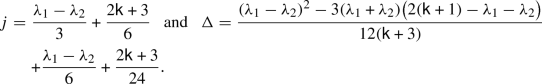  (4.9)

Moreover, the $\mathcal {H}_{j,\Delta }$ and $\mathcal {H}^{tw }_{j,\Delta }$ determined by the surviving weights are all mutually nonisomorphic.

In light of this classification, we let $\mathcal {H}_{\lambda } = \mathcal {H}_{j,\Delta }$ and $\mathcal {H}^{tw }_{\lambda } = \mathcal {H}^{tw }_{j,\Delta }$, where j and $\Delta$ are given in terms of $\lambda \in \Sigma _{\mathsf {u},\mathsf {v}}$ by (4.2) and (4.9), respectively. Note that this implies that

$$\begin{aligned} \mathcal {H}^{tw }_{\lambda } \simeq \sigma ^{1/2}(\mathcal {H}_{\lambda }), \end{aligned}$$

(4.10)

by Proposition 3.2. With this new notation, the vacuum module $\mathcal {H}_{0,0}$ is identified as $\mathcal {H}_{\lambda }$, where $\lambda = [k,0,0]$ has $\lambda ^I = [\mathsf {u}-3,0,0]$ and $\lambda ^F = [\mathsf {v}-1,0,0]$.

We record the following strengthening of Theorem 4.9, following [54, Thm. 10.10], for later use.

Theorem 4.10

Let $\mathsf {k}$ be as in Assumption 1. Then, every highest-weight -module, untwisted or twisted, is simple.

Proof

We prove this for untwisted modules as the twisted case follows immediately from (4.10) and the invertibility of spectral flow. Since the simple quotient of any highest-weight -module $\mathcal {H}_{}$ is isomorphic to some $\mathcal {H}_{\lambda }$ with $\lambda \in \Sigma _{\mathsf {u},\mathsf {v}}$, by Theorem 4.9, it is enough to show that $\mathcal {H}_{}$ cannot have a composition factor isomorphic to $\mathcal {H}_{\mu }$ for some $\mu \in \Sigma _{\mathsf {u},\mathsf {v}}$ distinct from $\lambda$. Indeed, it is enough to show that the Verma module $\mathcal {V}_{\lambda } = \mathcal {V}_{j,\Delta }$ of $\mathsf {BP}^{\mathsf {k}}$ does not have such a composition factor.

Recall that $\mathcal {K}_{\lambda }$ denotes the Verma module of of highest weight $\lambda$ and let $\bigl [ \mathcal {K}_{\lambda } : \mathcal {L}_{\nu } \bigr ]$ denote the multiplicity with which $\mathcal {L}_{\nu }$ appears as a composition factor of $\mathcal {K}_{\lambda }$. By Theorem 4.4, quantum hamiltonian reduction takes $\mathcal {K}_{\lambda }$ to $\mathcal {V}_{\lambda }$ and only $\mathcal {L}_{\mu }$ and $\mathcal {L}_{w_{0} \cdot \mu }$ are sent to $\mathcal {H}_{\mu }$. As reduction is exact, we must have $\bigl [ \mathcal {V}_{\lambda } : \mathcal {H}_{\mu } \bigr ] = \bigl [ \mathcal {K}_{\lambda } : \mathcal {L}_{\mu } \bigr ] + \bigl [ \mathcal {K}_{\lambda } : \mathcal {L}_{w_{0} \cdot \mu } \bigr ]$ (noting that $\mu$ and $w_{0} \cdot \mu$ are distinct since $\mu \in \Sigma _{\mathsf {u},\mathsf {v}}$).

It follows that if $\mathcal {V}_{\lambda }$ has $\mathcal {H}_{\mu }$, $\mu \ne \lambda$, as a composition factor, then $\mathcal {K}_{\lambda }$ has either $\mathcal {L}_{\mu }$ or $\mathcal {L}_{w_{0} \cdot \mu }$ as a composition factor. But, $\lambda$, $\mu$ and $w_{0} \cdot \mu$ are all admissible $\widehat{\mathfrak {sl}}_{3}$-weights (corresponding to , and $w_{1}$, respectively, see Lemma 4.6), hence they are dominant. This is therefore impossible by the linkage principle for Verma $\widehat{\mathfrak {sl}}_{3}$-modules. $\square$

Because the Bernšteĭn–Gel’fand–Gel’fand category $\mathscr {O}_{\mathsf {u},\mathsf {v}}$ of level-$\mathsf {k}$ -modules admits contragredient duals, it follows from Theorem 4.10 that every extension between $\mathcal {H}_{\lambda }$ and $\mathcal {H}_{\mu }$, with $\lambda \ne \mu$, splits. It is likewise easy to see that a nonsplit self-extension of $\mathcal {H}_{\lambda }$ requires a nonsemisimple action of $J_0$ or $L_0$ (which is forbidden in $\mathscr {O}_{\mathsf {u},\mathsf {v}}$). $\mathscr {O}_{\mathsf {u},\mathsf {v}}$ is thus semisimple and, by Theorem 4.9, has finitely many isomorphism classes of simple objects. We may therefore summarise this as follows: is rational in category $\mathscr {O}_{\mathsf {u},\mathsf {v}}$.

In order to extend the highest-weight classification of Theorem 4.9 to twisted relaxed highest-weight -modules, we need to know when the top space is infinite-dimensional. The condition for this is beautifully succinct when expressed in terms of surviving weights.

Proposition 4.11

The top space of the simple twisted highest-weight -module $\mathcal {H}^{tw }_{\lambda }$ is finite-dimensional if and only if $\lambda ^F_1 = 0$. When $\lambda ^F_1 = 0$, the dimension of this top space is $\lambda ^I_1 + 1$.

Proof

By Proposition 3.17, $(\mathcal {H}^{tw }_{j,\Delta })^{top }$ is finite-dimensional if and only if $h_{\mathsf {k}}^n(j,\Delta ) = 0$ for some $n \in \mathbb {Z}_{\geqslant 1}$ and, if it is finite-dimensional, then the dimension is the smallest such n. Substituting (4.9) into the definition (3.10) of $h_{\mathsf {k}}^n$ and simplifying, we find that

(4.11)

The only possible roots in $\mathbb {Z}_{\geqslant 1}$ are thus $n=\lambda _1+1$ and $n=\frac{\mathsf {u}}{\mathsf {v}}-\lambda _2-1$. As $\lambda = \lambda ^I - \frac{\mathsf {u}}{\mathsf {v}} \lambda ^F$, the former requires $\lambda _1 \in \mathbb {Z}$ so $\lambda ^F_1 = 0$ and $n = \lambda ^I_1+1 \in \mathbb {Z}_{\geqslant 1}$. On the other hand, the latter requires $n=-(\lambda ^I_2+1) + \frac{\mathsf {u}}{\mathsf {v}}(\lambda ^F_2+1)$ which is only an integer if $\lambda ^F_2 = \mathsf {v}-1$. However, this contradicts $\lambda ^F \in \mathsf {P}^{\mathsf {v}-1}_{\geqslant }$ and $\lambda ^F_0 \geqslant 1$ (Lemma 4.6). $\quad \square$

Corollary 4.12

Given $\mathsf {k}$ as in Assumption 1, there are (up to isomorphism):

• $\frac{1}{4} (\mathsf {u}-1)(\mathsf {u}-2)\mathsf {v}(\mathsf {v}-1)$ simple untwisted highest-weight -modules;

• $\frac{1}{2} (\mathsf {u}-1)(\mathsf {u}-2)(\mathsf {v}-1)$ simple twisted highest-weight -modules with finite-dimensional top spaces;

• $\frac{1}{4} (\mathsf {u}-1)(\mathsf {u}-2)(\mathsf {v}-1)(\mathsf {v}-2)$ simple twisted highest-weight -modules with infinite-dimensional top spaces;

In particular, there are no simple twisted highest-weight -modules with infinite-dimensional top spaces when $\mathsf {v}=2$. This is in accord with the fact that the with $\mathsf {u}\geqslant 3$ are rational [1].

Recall that the conjugation automorphism $\gamma$ of , given in (2.9), negates $J_0$ and preserves $L_0$. At the level of their eigenvalues, this is effected in (4.2) by exchanging the Dynkin labels $\lambda _1$ and $\lambda _2$ of $\lambda$. The result of this exchange is clearly still a surviving weight, by Lemma 4.6.

Proposition 4.13

For each $\lambda \in \Sigma _{\mathsf {u},\mathsf {v}}$, we have:

• $\gamma (\mathcal {H}_{[\lambda _0,\lambda _1,\lambda _2]}) \simeq \mathcal {H}_{[\lambda _0,\lambda _2,\lambda _1]}$.

• If $\lambda ^F_1 = 0$, then $\gamma (\mathcal {H}^{tw }_{\lambda }) \simeq \mathcal {H}^{tw }_{\mu }$, where $\mu = [\lambda _2 - \frac{\mathsf {u}}{\mathsf {v}}, \lambda _1, \lambda _0 + \frac{\mathsf {u}}{\mathsf {v}}]$, hence $\mu ^I = [\lambda ^I_2,\lambda ^I_1,\lambda ^I_0]$ and $\mu ^F = [\lambda ^F_2+1,0,\lambda ^F_0-1]$. Otherwise, $\gamma (\mathcal {H}^{tw }_{[\lambda _0,\lambda _1,\lambda _2]})$ is not highest-weight (though it is relaxed highest-weight).

Proof

The result of conjugating a simple untwisted highest-weight -module is clear from the above remarks, because the top spaces are one-dimensional. For the twisted case, first note that the conjugate of $\mathcal {H}^{tw }_{\lambda }$ will be again highest-weight if its top space is finite-dimensional (otherwise the top space of the conjugate module will be an infinite-dimensional lowest-weight $\mathsf {Z}_{\mathsf {k}}$-module). By Proposition 4.11, this requires $\lambda ^F_1 = 0$, hence $\lambda _1 = \lambda ^I_1$. Assuming this, let j and $\Delta$ denote the charge and conformal weight, respectively, of the highest-weight vector of $\mathcal {H}^{tw }_{\lambda }$. Then, the highest-weight vector of $\gamma (\mathcal {H}^{tw }_{\lambda })$ has charge $\lambda _1-j$ and conformal weight $\Delta$.

We therefore need to find $\mu \in \Sigma _{\mathsf {u},\mathsf {v}}$ corresponding to these eigenvalues under (4.9). Solving for $\mu$, we find two solutions:

(4.12)

We know from the proof of Lemma 4.6 that only one of these is a surviving weight and the other is a $w=w_{1}$ survivor obtained from the one by applying the shifted action of $w_{0}$. It is easy to check that the first solution is the survivor by writing it in the form

$$\begin{aligned} \mu _0 = \lambda ^I_2 - \frac{\mathsf {u}}{\mathsf {v}} (\lambda ^F_2+1), \quad \mu _1 = \lambda ^I_1 \quad \text {and} \quad \mu _2 = \lambda ^I_0 - \frac{\mathsf {u}}{\mathsf {v}} (\lambda ^F_0-1). \end{aligned}$$

(4.13)

Indeed, $\lambda ^F_0 \geqslant 1$ implies that $\mu ^I = [\lambda ^I_2,\lambda ^I_1,\lambda ^I_0] \in \mathsf {P}^{\mathsf {u}-3}_{\geqslant }$, $\mu ^F = [\lambda ^F_2+1,0,\lambda ^F_0-1] \in \mathsf {P}^{\mathsf {v}-1}_{\geqslant }$ and $\mu ^F_0 \geqslant 1$, hence that $\mu \in \Sigma _{\mathsf {u},\mathsf {v}}$. $\quad \square$

It remains to determine when the spectral flow of a simple highest-weight -module is another such module. By Proposition 3.2, it suffices to consider the untwisted case. Again the key is the finite-dimensionality of the top space: $\sigma ^{}(\mathcal {H}_{\lambda })$ will be highest-weight if and only if $\mathcal {H}^{tw }_{\lambda } = \sigma ^{1/2}(\mathcal {H}_{\lambda })$ has a finite-dimensional top space, that is if and only if $\lambda ^F_1 = 0$ (Proposition 4.11). Indeed, if $\lambda ^F_1 = 0$ and v denotes the highest-weight vector of $\mathcal {H}_{\lambda }$, then that of $\sigma ^{}(\mathcal {H}_{\lambda })$ is easily checked to be $(G^-_{1/2})^{\lambda ^I_1} \sigma ^{}(v)$. We compute its charge and conformal weight, then determine the (unique ) surviving weight that gives these eigenvalues under (4.2), as in the proof of Proposition 4.13. We thereby obtain the following proposition.

Proposition 4.14

If $\lambda \in \Sigma _{\mathsf {u},\mathsf {v}}$ satisfies $\lambda ^F_1 = 0$, then $\sigma ^{}(\mathcal {H}_{\lambda }) \simeq \mathcal {H}_{\mu }$, where $\mu = [\lambda _2 - \frac{\mathsf {u}}{\mathsf {v}}, \lambda _0 + \frac{\mathsf {u}}{\mathsf {v}}, \lambda _1] \in \Sigma _{\mathsf {u},\mathsf {v}}$, hence $\mu ^I = [\lambda ^I_2,\lambda ^I_0,\lambda ^I_1]$ and $\mu ^F = [\lambda ^F_2+1,\lambda ^F_0-1,0]$. If $\lambda ^F_1 \ne 0$, then $\sigma ^{}(\mathcal {H}_{\lambda })$ is not highest-weight (nor relaxed highest-weight).

Combining this with the dihedral relation (2.8) and Proposition 4.13, we obtain the following characterisation of the spectral flow orbit of a simple untwisted highest-weight -module $\mathcal {H}_{\lambda }$. We recall from Proposition 3.2 that a twisted member $\sigma ^{\ell +1/2}(\mathcal {H}_{\lambda })$, $\ell \in \mathbb {Z}$, of this orbit is highest-weight if and only if its untwisted predecessor $\sigma ^{\ell }(\mathcal {H}_{\lambda })$ is.

Theorem 4.15

Take $\lambda \in \Sigma _{\mathsf {u},\mathsf {v}}$ and define $\mu , \nu , {\bar{\mu }}, {\bar{\nu }} \in \Sigma _{\mathsf {u},\mathsf {v}}$ by

(4.14)

• $\sigma ^{}(\mathcal {H}_{\lambda })$ is highest-weight if and only if $\lambda ^F_1=0$. In this case, $\sigma ^{}(\mathcal {H}_{\lambda }) \simeq \mathcal {H}_{\mu }$.

• $\sigma ^{-1}(\mathcal {H}_{\lambda })$ is highest-weight if and only if $\lambda ^F_2=0$. In this case, $\sigma ^{-1}(\mathcal {H}_{\lambda }) \simeq \mathcal {H}_{{\bar{\mu }}}$.

• $\sigma ^{2}(\mathcal {H}_{\lambda })$ is highest-weight if and only if $\lambda ^F=[1,0,\mathsf {v}-2]$. In this case, $\sigma ^{2}(\mathcal {H}_{\lambda }) \simeq \mathcal {H}_{\nu }$.

• $\sigma ^{-2}(\mathcal {H}_{\lambda })$ is highest-weight if and only if $\lambda ^F=[1,\mathsf {v}-2,0]$. In this case, $\sigma ^{-2}(\mathcal {H}_{\lambda }) \simeq \mathcal {H}_{{\bar{\nu }}}$.

• For ${|}{\ell }{|} \in \mathbb {Z}_{\geqslant 3}$, $\sigma ^{\ell }(\mathcal {H}_{\lambda })$ is highest-weight if and only if $\mathsf {v}=2$. In this case, $\sigma ^{\pm 3}(\mathcal {H}_{\lambda }) \simeq \mathcal {H}_{\lambda }$.

Note that when $\mathsf {v}=2$, every $\lambda \in \Sigma _{\mathsf {u},\mathsf {v}}$ has $\lambda ^F = [1,0,0]$. The spectral flow orbits thus take the form

$$\begin{aligned} \cdots \overset{\sigma ^{1/2}}{\longmapsto }\mathcal {H}_{\lambda } \overset{\sigma ^{1/2}}{\longmapsto }\mathcal {H}^{tw }_{\lambda } \overset{\sigma ^{1/2}}{\longmapsto }\mathcal {H}_{\mu } \overset{\sigma ^{1/2}}{\longmapsto }\mathcal {H}^{tw }_{\mu } \overset{\sigma ^{1/2}}{\longmapsto }\mathcal {H}_{\nu } \overset{\sigma ^{1/2}}{\longmapsto }\mathcal {H}^{tw }_{\nu } \overset{\sigma ^{1/2}}{\longmapsto }\mathcal {H}_{\lambda } \overset{\sigma ^{1/2}}{\longmapsto }\cdots , \end{aligned}$$

(4.15)

where $\mu$ and $\nu$ are as in (4.14) (with $\mu ^F = \nu ^F = [1,0,0]$). We picture the $\mathsf {v}\geqslant 3$ spectral flow orbits in Figure 1.

Fig. 1

A picture of the weights of the three types of spectral flow orbits through a simple highest-weight -module with $\mathsf {v}\geqslant 3$. The charge increases from left to right, whilst the conformal weight increases from top to bottom. The given constraints on the Dynkin labels of $\lambda ^F$ must be satisfied by the simple untwisted highest-weight -module $\mathcal {H}_{\lambda }$ appearing at that point in the orbit. Note that the unpictured modules in each infinite orbit, indicated by $\cdots$, are neither highest-weight nor relaxed highest-weight: their conformal weights are unbounded below

4.3 Simple relaxed highest-weight -modules

As we noted in Theorem 3.11, every simple untwisted relaxed highest-weight -module is highest-weight. The classification of simple untwisted relaxed highest-weight modules was therefore completed in Theorem 4.9. It remains to classify the simple twisted relaxed highest-weight modules, specifically those whose top spaces are simple dense $\mathsf {Z}_{\mathsf {k}}$-modules (those whose top spaces are simple lowest-weight $\mathsf {Z}_{\mathsf {k}}$-modules are conjugates of the simple twisted highest-weight -modules classified in Theorem 4.9).

A simple twisted relaxed highest-weight $\mathsf {BP}^{\mathsf {k}}$-module $\mathcal {M}$ is a $\mathsf {BP}_{\mathsf {k}}$-module if and only if its top space is annihilated by , where $\mathsf {J}^{\mathsf {k}}$ denotes the maximal ideal of $\mathsf {BP}^{\mathsf {k}}$. An obvious consequence of Theorem 4.9 is that annihilates , with j and $\Delta$ determined by $\lambda$ as in (4.9), if and only if $\lambda \in \Sigma _{\mathsf {u},\mathsf {v}}$. We extend this to the simple relaxed highest-weight modules $\mathcal {R}^{tw }_{[j],\Delta ,\omega }$ of Theorem 3.23 using an argument similar to that of [24, Prop. 4.2].

Proposition 4.16

The irreducible semisimple coherent family $\overline{\mathcal {C}}_{\Delta ,\omega }^{ss }$ of $\mathsf {Z}_{\mathsf {k}}$-modules is a -module if and only if one of its infinite-dimensional submodules is.

Proof

Obviously, $\overline{\mathcal {C}}_{\Delta ,\omega }^{ss }$ being a -module implies that every one of its submodules are too, in particular the infinite-dimensional ones.

To prove the converse, we lean heavily on the general methodology developed in [24] to classify relaxed highest-weight modules for affine vertex operator algebras, though the argument here is easier because the relevant coherent families have one-dimensional weight spaces. The first step is to consider the subalgebra , where we recall that $\mathsf {C}_{\mathsf {k}}= \mathbb {C}[J,L,\Omega ]$ (Lemma 3.20). The relevance is that a simple weight -module $\mathcal {M}$ is a -module if and only if $\mathsf {A}_{\mathsf {k}}$ annihilates some nonzero element of $\mathcal {M}$. This fact is proved in exactly the same way that [24, Lem. 4.1] is (see also [55]) and so we omit the details.

We next note that the action of $\mathsf {A}_{\mathsf {k}}$ preserves each of the one-dimensional weight spaces of the irreducible semisimple coherent family $\overline{\mathcal {C}}_{\Delta ,\omega }^{ss }$ and that this action is polynomial: for each $a \in \mathsf {A}_{\mathsf {k}}\subset \mathbb {C}[J,L,\Omega ]$, there is a polynomial $p_a$ in three variables such that a acts on the weight space $\overline{\mathcal {C}}_{\Delta ,\omega }^{ss }(j,\Delta ,\omega )$ as multiplication by $p_a(j,\Delta ,\omega )$. Since $\Delta$ and $\omega$ are fixed by the choice of coherent family, we may regard $p_a$ as a single-variable polynomial.

If we now assume that one of the infinite-dimensional submodules of $\overline{\mathcal {C}}_{\Delta ,\omega }^{ss }$ is a -module, then it is annihilated by and thus by $\mathsf {A}_{\mathsf {k}}$. Thus, for every $a \in \mathsf {A}_{\mathsf {k}}$, we have $p_a(j,\Delta ,\omega ) = 0$ for infinitely many distinct values of j, whence $p_a({-},\Delta ,\omega )$ must be the zero polynomial. But, then a annihilates all of $\overline{\mathcal {C}}_{\Delta ,\omega }^{ss }$, whence $\overline{\mathcal {C}}_{\Delta ,\omega }^{ss }$ is a -module. $\square$

Note that the top space of every (simple) $\mathcal {R}^{tw }_{[j],\Delta ,\omega }$ embeds into some irreducible semisimple coherent family and that every such family has an infinite-dimensional highest-weight submodule $\overline{\mathcal {H}}_{j',\Delta }$, by Proposition 3.25. From Theorem 4.9, we have classified all the simple highest-weight -modules in terms of surviving weights. Proposition 4.16 thus determines the irreducible semisimple coherent families that are -modules and in this way we find all the $\mathcal {R}^{tw }_{[j],\Delta ,\omega }$ that are simple -modules. Algorithmically, this classification proceeds as follows.

Let $\Gamma _{\mathsf {u},\mathsf {v}}$ denote the set of () admissible $\widehat{\mathfrak {sl}}_{3}$-weights $\lambda$ of level $\mathsf {k}$ with $\lambda ^F_0 \ne 0$, so that $\lambda \in \Sigma _{\mathsf {u},\mathsf {v}}$ (Lemma 4.6), and $\lambda ^F_1 \ne 0$, so that $\mathcal {H}^{tw }_{\lambda }$ has an infinite-dimensional top space (Proposition 4.11). Then, $\Gamma _{\mathsf {u},\mathsf {v}}$ parametrises the isomorphism classes of the simple highest-weight -modules with infinite-dimensional top spaces.

• For each $\lambda \in \Gamma _{\mathsf {u},\mathsf {v}}$, compute j and $\Delta$ using (4.9), then substitute into (3.19) to compute $\omega$:

  

  (4.16)

  This gives the eigenvalues of J, L and $\Omega$ on the highest-weight vector of $(\mathcal {H}^{tw }_{\lambda })^{top }$.

• Then, the $\mathcal {R}^{tw }_{[j'],\Delta ,\omega }$ are, for all $[j'] \in \mathbb {C}/\mathbb {Z}$ satisfying $\omega ^+_{i,\Delta } \ne \omega$ for every $i \in [j']$, simple relaxed highest-weight -modules (by Theorem 3.23 and Proposition 4.16) and all such modules are obtained, up to isomorphism, in this way.

As with the highest-weight -modules classified in Sect. 4.2, it is convenient to let $\mathcal {R}^{tw }_{[j],\lambda } = \mathcal {R}^{tw }_{[j],\Delta ,\omega }$, where $\Delta$ and $\omega$ are given in terms of $\lambda$ by (4.9) and (4.16), respectively.

We may now summarise this classification as follows.

Theorem 4.17

Let $\mathsf {k}$ be as in Assumption 1 and let j be such that $\mathcal {R}^{tw }_{[j],\lambda }$ is simple. Then, $\mathcal {R}^{tw }_{[j],\lambda }$ is a (twisted) -module if and only if $\lambda \in \Gamma _{\mathsf {u},\mathsf {v}}$.

In fact, we shall see that a complete classification does not require considering every possible weight $\lambda \in \Gamma _{\mathsf {u},\mathsf {v}}$. First however, we recall from Corollary 4.12 that there are no highest-weight -modules with infinite-dimensional top spaces, hence $\Gamma _{\mathsf {u},\mathsf {v}}= \varnothing$, when $\mathsf {v}=2$.

Corollary 4.18

Let $\mathsf {k}$ be as in Assumption 1 with $\mathsf {v}=2$. Then, every simple (twisted) relaxed highest-weight -module is highest-weight.

Again, this is consistent with the fact [1] that is rational for every $\mathsf {u}\in 2\mathbb {Z}_{\geqslant 0}+3$. It is therefore convenient to slightly refine Assumption 1 as follows.

Assumption 2

In what follows, we shall restrict to fractional levels $\mathsf {k}= -3 + \frac{\mathsf {u}}{\mathsf {v}}$ with $\mathsf {u},\mathsf {v}\geqslant 3$.

The levels of Assumption 2 are also known as nondegenerate admissible levels in the literature. We shall understand that Assumption 2 is in force for the rest of this section.

Given an irreducible semisimple coherent family $\overline{\mathcal {C}}_{\Delta ,\omega }^{ss }$ of -modules, we ask how many inequivalent infinite-dimensional highest-weight submodules it possesses. By Proposition 3.21, the direct summands $\overline{\mathcal {R}}_{[j],\Delta ,\omega }$ are not simple for at least one, and at most three, $[j] \in \mathbb {C}/\mathbb {Z}$ and each nonsimple summand has precisely one infinite-dimensional highest-weight submodule. The answer to our question is therefore either one, two or three. In fact, for $\mathsf {k}$ as in Assumption 2, the answer is always three.

Lemma 4.19

If $\mathsf {k}$ is as in Assumption 2, then each irreducible semisimple coherent family $\overline{\mathcal {C}}_{\Delta ,\omega }^{ss }$ of -modules has precisely three infinite-dimensional highest-weight submodules. The map $\Gamma _{\mathsf {u},\mathsf {v}}\rightarrow \mathbb {C}^2$ given by $\lambda \mapsto (\Delta ,\omega )$ is thus 3-to-1. Moreover, the highest weights $\lambda = \lambda ^I - \frac{\mathsf {u}}{\mathsf {v}} \lambda ^F$ of these three submodules are related by the following $\mathbb {Z}_3$-action:

$$\begin{aligned} \begin{aligned}&\cdots \longmapsto [\lambda _0,\lambda _1,\lambda _2] \longmapsto [\lambda _2 - \tfrac{\mathsf {u}}{\mathsf {v}},\lambda _0,\lambda _1 + \tfrac{\mathsf {u}}{\mathsf {v}}] \longmapsto [\lambda _1,\lambda _2 - \tfrac{\mathsf {u}}{\mathsf {v}},\lambda _0 + \tfrac{\mathsf {u}}{\mathsf {v}}] \longmapsto \cdots ,\\&\qquad \cdots \longmapsto [\lambda ^I_0,\lambda ^I_1,\lambda ^I_2] \longmapsto [\lambda ^I_2,\lambda ^I_0,\lambda ^I_1] \longmapsto [\lambda ^I_1,\lambda ^I_2,\lambda ^I_0] \longmapsto \cdots , \\&\cdots \longmapsto [\lambda ^F_0,\lambda ^F_1,\lambda ^F_2] \longmapsto [\lambda ^F_2+1,\lambda ^F_0,\lambda ^F_1-1] \longmapsto [\lambda ^F_1,\lambda ^F_2+1,\lambda ^F_0-1] \longmapsto \cdots . \end{aligned} \end{aligned}$$

(4.17)

Proof

It is easy to see from (4.17) that if $\lambda \in \Gamma _{\mathsf {u},\mathsf {v}}$, then so do its images under the $\mathbb {Z}_3$-action. The three highest-weight modules corresponding to the $\mathbb {Z}_3$-orbit are thus -modules with infinite-dimensional top spaces if any is. Moreover, substituting $\lambda _1 \mapsto \lambda _0 = \mathsf {k}- \lambda _1 - \lambda _2$ and $\lambda _2 \mapsto \lambda _1 + \mathsf {k}+3$ into (4.9) and (4.16) shows that $\Delta$ and $\omega$ are invariant under this $\mathbb {Z}_3$-action. The three highest-weight modules therefore arise as submodules of the same irreducible semisimple coherent family. These modules are mutually inequivalent because their highest weights can only coincide if $\lambda ^I_0 = \lambda ^I_1 = \lambda ^I_2 = \frac{\mathsf {u}-3}{3}$ and $\lambda ^F_0 = \lambda ^F_1 = \lambda ^F_2 + 1 = \frac{\mathsf {v}}{3}$. But, this requires both $\mathsf {u}$ and $\mathsf {v}$ to be divisible by 3. $\square$

From Corollary 4.12, we now have a precise count of the number of irreducible semisimple coherent families of -modules. Each direct summand of such a family is the top space of a simple twisted relaxed highest-weight -module, by Theorem 3.13. With Equation (2.9), Lemma 3.20, and Proposition 4.16, we have the following theorem.

Theorem 4.20

Let $\mathsf {k}$ be as in Assumption 2. Then:

• There are $\frac{1}{3} {|}{\Gamma _{\mathsf {u},\mathsf {v}}}{|} = \frac{1}{12} (\mathsf {u}-1)(\mathsf {u}-2)(\mathsf {v}-1)(\mathsf {v}-2)$ irreducible semisimple coherent families of -modules $\overline{\mathcal {C}}_{\Delta ,\omega }^{ss }$, up to isomorphism.

• The families of twisted relaxed highest-weight -modules $\mathcal {R}^{tw }_{[j],\lambda } = \mathcal {R}^{tw }_{[j],\Delta ,\omega }$ are in 1-to-1 correspondence with $\Gamma _{\mathsf {u},\mathsf {v}}/ \mathbb {Z}_3$, where $\mathbb {Z}_3$ acts freely as in (4.17).

• For each $\lambda \in \Gamma _{\mathsf {u},\mathsf {v}}$, the twisted relaxed highest-weight module $\mathcal {R}^{tw }_{[j],\lambda }$ is a simple -module for all cosets $[j] \in \mathbb {C}/\mathbb {Z}$ except three, namely the three distinct cosets that contain a root i of the polynomial $\omega ^+_{i,\Delta } - \omega$.

• The conjugate of the simple twisted relaxed highest-weight -module $\mathcal {R}^{tw }_{[j],\Delta ,\omega }$ is $\gamma (\mathcal {R}^{tw }_{[j],\Delta ,\omega }) \simeq \mathcal {R}^{tw }_{[-j],\Delta ,-\omega }$.

Note that if $(\Delta ,\omega )$ corresponds to a coherent family of -modules, then the conjugation functor requires that so must $(\Delta ,-\omega )$. In fact, it is easy to check that $\Delta$ is invariant and $\omega$ is antiinvariant under the $\mathbb {Z}_2$-action $[\lambda _0,\lambda _1,\lambda _2] \leftrightarrow [\lambda _2 - \frac{\mathsf {u}}{\mathsf {v}},\lambda _1,\lambda _0 + \frac{\mathsf {u}}{\mathsf {v}}]$, that is

$$\begin{aligned} {[}\lambda ^I_0,\lambda ^I_1,\lambda ^I_2] \longleftrightarrow [\lambda ^I_2,\lambda ^I_1,\lambda ^I_0], \quad [\lambda ^F_0,\lambda ^F_1,\lambda ^F_2] \longleftrightarrow [\lambda ^F_2+1,\lambda ^I_1,\lambda ^I_0-1], \end{aligned}$$

(4.18)

which obviously preserves belonging to $\Gamma _{\mathsf {u},\mathsf {v}}$. With (4.17), this defines an action of $\mathsf {W}= \mathsf {S}_3$ on $\Gamma _{\mathsf {u},\mathsf {v}}$. The orbits clearly have length 6 unless $\omega =0$, in which case Lemma 4.19 forces them to have length 3. It is easy to check that this is consistent with the explicit factorisation of $\omega$ given in (4.16).

We remark that the spectral flow images $\sigma ^{\ell }(\mathcal {R}^{tw }_{[j],\lambda })$, $\ell \ne 0$, of these simple twisted relaxed highest-weight -modules are likewise simple -modules, but they are not relaxed highest-weight because their conformal weights are not bounded below.

4.4 Nonsimple relaxed highest-weight -modules

In Sect. 3.6, we introduced three classes of irreducible coherent families of $\mathsf {Z}_{\mathsf {k}}$-modules. The first, the semisimple class, was the key ingredient in the classification arguments of the previous section. Here, we will analyse the other two classes in order to demonstrate the existence of certain nonsemisimple twisted relaxed highest-weight -modules, assuming that $\mathsf {k}$ is as in Assumption 2. We will also describe the structure of these nonsemisimple modules in terms of short exact sequences.

Consider therefore the irreducible nonsemisimple coherent family $\overline{\mathcal {C}}_{\Delta ,\omega }^{\,\pm }$ of $\mathsf {Z}_{\mathsf {k}}$-modules on which $G^{\pm }$ acts injectively. Recall that its simple direct summands are the $\overline{\mathcal {R}}_{[j],\Delta ,\omega }$, for all but (up to) three $[j] \in \mathbb {C}/\mathbb {Z}$, and that its nonsimple direct summands are denoted by $\overline{\mathcal {R}}_{[j],\Delta ,\omega }^{\,\pm }$. We begin by determining the structure of these nonsimple $\mathsf {Z}_{\mathsf {k}}$-modules in the case relevant to studying -modules.

Proposition 4.21

Let $\lambda \in \Gamma _{\mathsf {u},\mathsf {v}}$ and let j, $\Delta$ and $\omega$ be defined by (4.9) and (4.16). Then, the nonsimple $\mathsf {Z}_{\mathsf {k}}$-module $\overline{\mathcal {R}}_{[j],\Delta ,\omega }^{\,\pm }$ has exactly two composition factors, $\overline{\mathcal {H}}_{j,\Delta }$ and $\overline{\gamma }(\overline{\mathcal {H}}_{-j-1,\Delta })$, both of which are -modules. Moreover, we have the following nonsplit short exact sequences:

$$\begin{aligned}&0 \longrightarrow \overline{\gamma }(\overline{\mathcal {H}}_{-j-1,\Delta }) \overset{}{\longrightarrow } \overline{\mathcal {R}}_{[j],\Delta ,\omega }^{\,+} \overset{}{\longrightarrow } \overline{\mathcal {H}}_{j,\Delta } \longrightarrow 0,\nonumber \\&\quad 0 \longrightarrow \overline{\mathcal {H}}_{j,\Delta } \overset{}{\longrightarrow } \overline{\mathcal {R}}_{[j],\Delta ,\omega }^{\,-} \overset{}{\longrightarrow } \overline{\gamma }(\overline{\mathcal {H}}_{-j-1,\Delta }) \longrightarrow 0. \end{aligned}$$

(4.19)

Proof

We only consider $\overline{\mathcal {R}}_{[j],\Delta ,\omega }^{\,+}$ as the argument for $\overline{\mathcal {R}}_{[j],\Delta ,\omega }^{\,-}$ is identical. First, note that $\overline{\mathcal {H}}_{j,\Delta }$ is an infinite-dimensional -module, by Theorem 4.9. The irreducible semisimple coherent family $\overline{\mathcal {C}}_{\Delta ,\omega }^{ss }$ is therefore a -module too, by Proposition 4.16, hence so is the lowest-weight module $\overline{\gamma }(\overline{\mathcal {H}}_{-j-1,\Delta }) \subset \overline{\mathcal {R}}_{[j],\Delta ,\omega }^{ss }$. As $\overline{\mathcal {R}}_{[j],\Delta ,\omega }^{ss }$ is the semisimplification of $\overline{\mathcal {R}}_{[j],\Delta ,\omega }^{\,+}$, they have the same composition factors. To demonstrate that there are no more factors beyond the two already found, it suffices to show that $\overline{\mathcal {H}}_{-j-1,\Delta }$ is infinite-dimensional.

Since the conjugate of $\overline{\mathcal {H}}_{-j-1,\Delta }$ is a -module, $\overline{\mathcal {H}}_{-j-1,\Delta }$ must correspond to some $\mu \in \Sigma _{\mathsf {u},\mathsf {v}}$, by Theorem 4.9. Proceeding as in the proof of Lemma 4.6, we find that the unique solution is $\mu = [\lambda _0, \lambda _2 - \frac{\mathsf {u}}{\mathsf {v}}, \lambda _1 + \frac{\mathsf {u}}{\mathsf {v}}]$, hence $\mu ^I = [\lambda ^I_0, \lambda ^I_2, \lambda ^I_1]$ and $\mu ^F = [\lambda ^F_0, \lambda ^F_2+1, \lambda ^F_1-1]$. Because $\mu ^F_1 = \lambda ^F_2+1 \ne 0$, it follows that $\mu \in \Gamma _{\mathsf {u},\mathsf {v}}$ and so $\overline{\mathcal {H}}_{-j-1,\Delta }$ is infinite-dimensional, as desired. This establishes the first exact sequence in (4.19). It is clearly nonsplit because $G^+$ acts injectively on $\overline{\mathcal {R}}_{[j],\Delta ,\omega }^{\,+}$. $\square$

At this point, it is not clear if the $\overline{\mathcal {R}}_{[j],\Delta ,\omega }^{\,\pm }$ corresponding to $\lambda \in \Gamma _{\mathsf {u},\mathsf {v}}$ are -modules, even though their composition factors are. We settle this using a simplified version of the argument of [24, Thm. 5.3].

Proposition 4.22

Let $\lambda \in \Gamma _{\mathsf {u},\mathsf {v}}$ and let j, $\Delta$ and $\omega$ be defined by (4.9) and (4.16). Then, the nonsimple $\mathsf {Z}_{\mathsf {k}}$-module $\overline{\mathcal {R}}_{[j],\Delta ,\omega }^{\,\pm }$ is a -module.

Proof

Again, we shall only detail the argument for $\overline{\mathcal {R}}_{[j],\Delta ,\omega }^{\,+}$. Recall that $\mathsf {J}^{\mathsf {k}}$ denotes the maximal ideal of $\mathsf {BP}^{\mathsf {k}}$ and so , by virtue of $\overline{\mathcal {H}}_{j,\Delta }$ being a -module. From the first exact sequence in (4.19), we conclude that .

As $\mathsf {Z}_{\mathsf {k}}$ is noetherian (this is an easy generalisation of [37, Cor. 1.3]), so is its quotient (Proposition 3.15). The ideal is therefore generated by a finite number of elements $a_1, \dots , a_n$ which we may, without loss of generality, choose to be eigenvectors of J. Let $j_i$ denote the J-eigenvalue of $a_i$, $i=1,\dots ,n$.

Choose $j' \in [j]$ such that . Then, $a_i$ takes the J-eigenspace of $\overline{\mathcal {R}}_{[j],\Delta ,\omega }^{\,+}$ of eigenvalue $j'$ into the J-eigenspace of $\overline{\gamma }(\overline{\mathcal {H}}_{-j-1,\Delta })$ of eigenvalue $j'+a_i \leqslant j$. But, the eigenvalues of J acting on $\overline{\gamma }(\overline{\mathcal {H}}_{-j-1,\Delta })$ are bounded below by $j+1$, hence $a_i$ annihilates the J-eigenspace of $\overline{\mathcal {R}}_{[j],\Delta ,\omega }^{\,+}$ of eigenvalue $j'$, for each i. It follows that annihilates this eigenspace. But, this eigenspace generates $\overline{\mathcal {R}}_{[j],\Delta ,\omega }^{\,+}$, hence (being an ideal) annihilates $\overline{\mathcal {R}}_{[j],\Delta ,\omega }^{\,+}$. $\square$

By Zhu-induction (Theorem 3.13), one may construct from each -module $\overline{\mathcal {R}}_{[j],\Delta ,\omega }^{\,\pm }$ a twisted -module whose twisted Zhu image (its top space) is $\overline{\mathcal {R}}_{[j],\Delta ,\omega }^{\,\pm }$. Consider the submodule of this induced module obtained by summing all the submodules whose intersection with the top space $\overline{\mathcal {R}}_{[j],\Delta ,\omega }^{\,\pm }$ is zero. Quotienting by this submodule results in a twisted -module, which we shall denote by $\mathcal {R}^{tw ,\pm }_{[j],\lambda } = \mathcal {R}^{tw ,\pm }_{[j],\Delta ,\omega }$, that has $\overline{\mathcal {R}}_{[j],\Delta ,\omega }^{\,\pm }$ as its top space and has the property that its nonzero submodules intersect this top space nontrivially. In a sense, $\mathcal {R}^{tw ,\pm }_{[j],\Delta ,\omega }$ is the smallest -module whose top space is $\overline{\mathcal {R}}_{[j],\Delta ,\omega }^{\,\pm }$.

The $\mathcal {R}^{tw ,\pm }_{[j],\lambda }$ are clearly nonsemisimple, because their top spaces are. This proves the following result.

Theorem 4.23

When $\mathsf {k}$ is as in Assumption 2, the simple vertex operator algebra admits nonsemisimple modules. In physical language, the corresponding minimal model conformal field theory is logarithmic.

As we have mentioned before, the Bershadsky–Polyakov minimal models corresponding to , with $\mathsf {u}\in 2\mathbb {Z}_{\geqslant 0}+3$, were shown to be rational in [1].

Our final task is then to determine the structure of these nonsemisimple -modules. For this, it is convenient to introduce new modules $\mathcal {W}^{tw ,\pm }_{[j],\lambda } = \mathcal {W}^{tw ,\pm }_{[j],\Delta ,\omega }$ that are obtained by treating $\overline{\mathcal {R}}_{[j],\Delta ,\omega }^{\,\pm }$ as a module over the twisted mode algebra $\mathsf {U}^{tw }_0$ of (3.1), letting $\mathsf {U}^{tw }_>$ act as 0, and then inducing to a $\mathsf {U}^{tw }$-module. It follows that $\mathcal {W}^{tw ,\pm }_{[j],\lambda }$ is a “relaxed Verma” $\mathsf {BP}^{\mathsf {k}}$-module whose top space is $\overline{\mathcal {R}}_{[j],\Delta ,\omega }^{\,\pm }$. In a sense, it is the largest $\mathsf {BP}^{\mathsf {k}}$-module with this top space.

As such, we may consider the sum $\mathcal {N}^{tw ,\pm }_{[j],\lambda }$ of all the submodules of $\mathcal {W}^{tw ,\pm }_{[j],\lambda }$ whose intersection with the top space $\overline{\mathcal {R}}_{[j],\Delta ,\omega }^{\,\pm }$ is zero. Because this top space is nonsemisimple, $\mathcal {N}^{tw ,\pm }_{[j],\lambda }$ is a proper submodule of the maximal submodule $\mathcal {M}^{tw ,\pm }_{[j],\lambda }$ of $\mathcal {W}^{tw ,\pm }_{[j],\lambda }$. Its utility lies in the fact that it provides an alternative construction of the -module $\mathcal {R}^{tw ,\pm }_{[j],\lambda }$:

$$\begin{aligned} \mathcal {R}^{tw ,\pm }_{[j],\lambda } \simeq \mathcal {W}^{tw ,\pm }_{[j],\lambda } \Big / \mathcal {N}^{tw ,\pm }_{[j],\lambda }. \end{aligned}$$

(4.20)

This exploits the fact that $\mathcal {R}^{tw ,\pm }_{[j],\lambda }$ is, in a sense, the smallest $\mathsf {BP}^{\mathsf {k}}$-module with top space $\overline{\mathcal {R}}_{[j],\Delta ,\omega }^{\,\pm }$.

We now proceed in an analogous fashion to [19, Sec. 4].

Theorem 4.24

Let $\mathsf {k}$ be as in Assumption 2 and let $\lambda \in \Gamma _{\mathsf {u},\mathsf {v}}$ define j, $\Delta$ and $\omega$ via (4.9) and (4.16). We then have the following nonsplit short exact sequences of -modules:

$$\begin{aligned}&0 \longrightarrow \gamma (\mathcal {H}^{tw }_{-j-1,\Delta }) \overset{}{\longrightarrow } \mathcal {R}^{tw ,+}_{[j],\Delta ,\omega } \overset{}{\longrightarrow } \mathcal {H}^{tw }_{j,\Delta } \longrightarrow 0,\nonumber \\&\qquad 0 \longrightarrow \mathcal {H}^{tw }_{j,\Delta } \overset{}{\longrightarrow } \mathcal {R}^{tw ,-}_{[j],\Delta ,\omega } \overset{}{\longrightarrow } \gamma (\mathcal {H}^{tw }_{-j-1,\Delta }) \longrightarrow 0. \end{aligned}$$

(4.21)

Proof

Once again, we only give the argument for $\mathcal {R}^{tw ,+}_{[j],\Delta ,\omega }$. First, note that the twisted Verma module $\mathcal {V}^{tw }_{j,\Delta }$ is clearly isomorphic to the quotient $\mathcal {W}^{tw ,+}_{[j],\Delta ,\omega } \big / \gamma (\mathcal {V}^{tw }_{-j-1,\Delta })$, by (4.19) and the exactness of induction. Hence, $\mathcal {H}^{tw }_{j,\Delta }$ is also a quotient and (4.20) gives

$$\begin{aligned} \frac{\mathcal {R}^{tw ,+}_{[j],\Delta ,\omega }}{\mathcal {M}^{tw ,+}_{[j],\Delta ,\omega } \big / \mathcal {N}^{tw ,+}_{[j],\Delta ,\omega }} \simeq \frac{\mathcal {W}^{tw ,+}_{[j],\Delta ,\omega }}{\mathcal {M}^{tw ,+}_{[j],\Delta ,\omega }} \simeq \mathcal {H}^{tw }_{j,\Delta }, \end{aligned}$$

(4.22)

since relaxed highest-weight modules have unique irreducible quotients. Thus, $\mathcal {H}^{tw }_{j,\Delta }$ is a quotient of $\mathcal {R}^{tw ,+}_{[j],\Delta ,\omega }$.

Next, note that the (unique) maximal submodule of $\gamma (\mathcal {V}^{tw }_{-j-1,\Delta })$ is $\gamma (\mathcal {V}^{tw }_{-j-1,\Delta }) \cap \mathcal {N}^{tw ,+}_{[j],\Delta ,\omega }$, because the only submodule of $\gamma (\mathcal {V}^{tw }_{-j-1,\Delta })$ intersecting its top space nontrivially is $\gamma (\mathcal {V}^{tw }_{-j-1,\Delta })$ itself. We therefore have

$$\begin{aligned} \gamma (\mathcal {H}^{tw }_{-j-1,\Delta }) = \frac{\gamma (\mathcal {V}^{tw }_{-j-1,\Delta })}{\gamma (\mathcal {V}^{tw }_{-j-1,\Delta }) \cap \mathcal {N}^{tw ,+}_{[j],\Delta ,\omega }} \simeq \frac{\gamma (\mathcal {V}^{tw }_{-j-1,\Delta }) + \mathcal {N}^{tw ,+}_{[j],\Delta ,\omega }}{\mathcal {N}^{tw ,+}_{[j],\Delta ,\omega }}, \end{aligned}$$

(4.23)

which is clearly a submodule of $\mathcal {W}^{tw ,+}_{[j],\Delta ,\omega } \big / \mathcal {N}^{tw ,+}_{[j],\Delta ,\omega } \simeq \mathcal {R}^{tw ,+}_{[j],\Delta ,\omega }$. Thus, $\gamma (\mathcal {H}^{tw }_{-j-1,\Delta })$ embeds into $\mathcal {R}^{tw ,+}_{[j],\Delta ,\omega }$.

To demonstrate exactness of the first sequence of (4.21), we note that

(4.24)

using (4.20) and (4.23). This shows that $\mathcal {R}^{tw ,+}_{[j],\Delta ,\omega } \big / \gamma (\mathcal {H}^{tw }_{-j-1,\Delta })$ is a twisted highest-weight -module. By Theorem 4.10, it is simple and therefore isomorphic to $\mathcal {H}^{tw }_{j,\Delta }$, by (4.22). This completes the proof. $\square$

5 Examples

We conclude by illustrating the above classification results with some specific examples of Bershadsky–Polyakov minimal models. The examples with $\mathsf {v}=2$ extend the results of [1] whilst the $(\mathsf {u},\mathsf {v}) = (3,4)$ and (4, 3) examples extend those of [2].

5.1 Example:

For $\mathsf {k}=-\frac{3}{2}$, the central charge of the minimal model is $\mathsf {c}=0$. Since and $\lambda ^F \in \mathsf {P}^{1}_{\geqslant }$ is constrained by $\lambda ^F_0 \geqslant 0$ so that $\lambda ^F = [1,0,0]$, we only have $\lambda = [0,0,0] - \frac{3}{2} [1,0,0] = [\mathsf {k},0,0]$. There is therefore a unique simple untwisted highest-weight module $\mathcal {H}_{-3 \omega _{0}/2} = \mathcal {H}_{0,0}$ and a unique simple twisted highest-weight module $\mathcal {H}^{tw }_{-3 \omega _{0}/2} = \mathcal {H}^{tw }_{0,0}$ (up to isomorphism). This is clearly the trivial minimal model.

5.2 Example:

For $\mathsf {k}=-\frac{1}{2}$, the central charge is instead $\mathsf {c}=\frac{2}{5}$ and we have $\lambda ^I \in \mathsf {P}^{2}_{\geqslant }$ and $\lambda ^F = [1,0,0]$. There are thus ${|}{\mathsf {P}^{2}_{\geqslant }}{|} = 6$ simple untwisted highest-weight modules and so 6 simple twisted highest-weight modules, all with finite-dimensional top spaces. We illustrate these modules in Figure 2, arranging them according to $\lambda ^I$ and listing the charges and conformal weights of their highest-weight vectors. We also indicate the effect of the conjugation and spectral flow automorphisms in this arrangement.

Fig. 2

The charges and conformal weights $(j,\Delta )$ of the untwisted (left) and twisted (right) simple highest-weight -modules, arranged by the Dynkin labels of the integral parts $\lambda ^I$ of the corresponding surviving weights $\lambda$. The subscript on the twisted labels gives the dimension of the top space. Conjugation $\gamma$ is indicated by reflection about the dashed line and spectral flow $\sigma$ by $120^{\circ }$ anticlockwise rotation about each triangle’s centre

5.3 Example:

We discuss one further minimal model with $\mathsf {v}=2$, that with $\mathsf {k}=\frac{3}{2}$ and $\mathsf {c}=-\frac{22}{3}$. This time, there are ${|}{\mathsf {P}^{6}_{\geqslant }}{|} = 28$ simple untwisted highest-weight modules and, of course, each has a single twisted cousin. As always when $\mathsf {v}=2$, the top spaces are all finite-dimensional and the fractional part $\lambda ^F$ of the corresponding $\widehat{\mathfrak {sl}}_{3}$-weights is [1, 0, 0].

An interesting feature of this minimal model is that the (integer) spectral flows of the vacuum module $\mathcal {H}_{0,0}$ correspond to $\lambda ^I = [0,6,0]$ and [0, 0, 6], hence $(j,\Delta ) = (2,1)$ and $(-2,1)$. Recalling that spectral flows of the vacuum module are always simple currents [56], it follows that admits an order-3 simple current extension $\mathsf {A}$. Moreover, if E and F denote the highest-weight vectors of the simple current modules $\mathcal {H}_{2,1}$ and $\mathcal {H}_{-2,1}$, respectively, then it is easy to check that E, F and J define a (nonconformal) embedding of the $\mathfrak {sl}_{2}$ minimal model into $\mathsf {A}$.

Defining $\overline{G}^{\,+} = G^-_{-1/2} E$ and $\overline{G}^{\,-} = G^+_{-1/2} F$, we see that $\mathsf {A}$ has four linearly independent fields of conformal weight $\frac{3}{2}$ and that they decompose into two $\mathfrak {sl}_{2}$-doublets $(G^-,\overline{G}^{\,+})$ and $(\overline{G}^{\,-},G^+)$. $\mathsf {A}$ may thus be regarded as some sort of bosonic analogue of the $N=4$ superconformal vertex operator superalgebra, see Figure 3. However, a major difference is that the elements E, J, F, $G^{\pm }$ $\overline{G}^{\,\pm }$ and L do not strongly generate $\mathsf {A}$. For example, the singular part of the operator product expansion of $G^+(z)$ and $\overline{G}^{\,-}(w)$ is a simple pole whose coefficient is the $(j,\Delta ) = (0,2)$ field corresponding to $T^- = (G^+_{-1/2})^2 F$.

Fig. 3

The states with conformal weight $\Delta \leqslant 2$ of the “$N=4$-like” vertex operator algebra $\mathsf {A} = \mathcal {H}_{-2,1} \oplus \mathcal {H}_{0,0} \oplus \mathcal {H}_{2,1}$ that extends . Here, $T^+ = G^-_{-1/2} \overline{G}^{\,+}$ and $T^- = G^+_{-1/2} \overline{G}^{\,-}$

It is nevertheless easy to explore the representation theory of $\mathsf {A}$. The set of 28 (isomorphism classes of) simple untwisted highest-weight -modules decomposes into 10 spectral flow orbits: 9 of length 3 and one fixed point. It is easy to check from the charges and conformal weights that only four of these orbits define untwisted $\mathsf {A}$-modules. There are therefore precisely 4 simple untwisted $\mathsf {A}$-modules:

$$\begin{aligned}&\mathsf {A} = \mathcal {H}_{-2,1} \oplus \mathcal {H}_{0,0} \oplus \mathcal {H}_{2,1}, \quad \mathcal {H}_{-1,1/6} \oplus \mathcal {H}_{0,-1/3} \oplus \mathcal {H}_{1,1/6}, \nonumber \\&\quad \mathcal {H}_{-1,-1/6} \oplus \mathcal {H}_{0,1/3} \oplus \mathcal {H}_{1,-1/6} \quad \text {and} \quad \mathcal {H}_{0,-2/9}. \end{aligned}$$

(5.1)

One can also classify the simple twisted $\mathsf {A}$-modules, but now there are several more twisted sectors to consider.

5.4 Example:

Consider next the Bershadsky–Polyakov minimal model with $\mathsf {k}=-\frac{9}{4}$ and $\mathsf {c}=-\frac{23}{2}$. This model arises as the $p=4$ member of a series $\mathcal {B}_p$ of interesting vertex operator algebras constructed in [57]. As $\lambda ^I \in \mathsf {P}^{0}_{\geqslant }$ and $\lambda ^F \in \mathsf {P}^{3}_{\geqslant }$ satisfies $\lambda ^F_0 \geqslant 1$, there are ${|}{\mathsf {P}^{2}_{\geqslant }}{|} = 6$ simple untwisted highest-weight modules and 6 simple twisted highest-weight modules, 3 of which have finite-dimensional top spaces. We illustrate these in Figure 4 as we did for , but arranging the data according to $\lambda ^F$ instead of $\lambda ^I$. One can check that this recovers the highest-weight classification of [2].

In this illustration, the spectral flow functor $\sigma$ is again represented by a $120^{\circ }$ anticlockwise rotation, but does not preserve being highest-weight (because $\mathsf {v}\ne 2$). Indeed, the three spectral flow orbits through the simple highest-weight -modules are

$$\begin{aligned} \begin{array}{c} \cdots \overset{\sigma ^{1/2}}{\longmapsto }\mathcal {H}_{0,-1/2} \overset{\sigma ^{1/2}}{\longmapsto }\mathcal {H}^{tw }_{-1/4,-9/16} \overset{\sigma ^{1/2}}{\longmapsto }\cdots , \\ \cdots \overset{\sigma ^{1/2}}{\longmapsto }\mathcal {H}_{1/4,-3/8} \overset{\sigma ^{1/2}}{\longmapsto }\mathcal {H}^{tw }_{0,-5/16} \overset{\sigma ^{1/2}}{\longmapsto }\mathcal {H}_{-1/4,-3/8} \overset{\sigma ^{1/2}}{\longmapsto }\mathcal {H}^{tw }_{-1/2,-9/16} \overset{\sigma ^{1/2}}{\longmapsto }\cdots , \\ \cdots \overset{\sigma ^{1/2}}{\longmapsto }\mathcal {H}_{1/2,-1/4} \overset{\sigma ^{1/2}}{\longmapsto }\mathcal {H}^{tw }_{1/4,-1/16} \overset{\sigma ^{1/2}}{\longmapsto }\mathcal {H}_{0,0} \overset{\sigma ^{1/2}}{\longmapsto }\mathcal {H}^{tw }_{-1/4,-1/16} \overset{\sigma ^{1/2}}{\longmapsto }\mathcal {H}_{-1/2,-1/4} \overset{\sigma ^{1/2}}{\longmapsto }\mathcal {H}^{tw }_{-3/4,-9/16} \overset{\sigma ^{1/2}}{\longmapsto }\cdots , \end{array} \end{aligned}$$

(5.2)

where the $\cdots$ indicate simple -modules that are not highest-weight.

Fig. 4

The charges and conformal weights $(j,\Delta )$ of the untwisted (left) and twisted (right) simple highest-weight -modules, arranged by the Dynkin labels of the fractional parts $\lambda ^F$ of the corresponding surviving weights $\lambda$. The subscript on the twisted labels gives the dimension of the top space. Conjugation $\gamma$ is indicated by reflection about the dashed line, restricted to the modules with finite-dimensional top spaces (the conjugate of a highest-weight module with an infinite-dimensional top space is not highest-weight)

The three simple twisted highest-weight modules with $\lambda ^F_1 > 0$ have infinite-dimensional top spaces. They also share the same conformal weight $\Delta = -\frac{9}{16}$ and $\omega$-parameter $\omega = \omega ^+_{j,\Delta } = 0$, the latter computed as in (4.16). It therefore follows that admits one family of simple twisted relaxed highest-weight modules $\mathcal {R}^{tw }_{[j],-9/16,0}$, $j \ne -\frac{1}{4}, -\frac{1}{2}, -\frac{3}{4} \pmod {1}$, as per Theorem 4.20. As a consistency check, substituting $\mathsf {k}=-\frac{9}{4}$ and $\Delta = -\frac{9}{16}$ into (3.19) indeed gives

$$\begin{aligned} \omega ^+_{j,-9/16} - \omega = (2j+1)(j^2+j+\tfrac{3}{16}) - 0 = 2(j+\tfrac{1}{4})(j+\tfrac{1}{2})(j+\tfrac{3}{4}), \end{aligned}$$

(5.3)

as expected.

This family was first constructed in [2, Thm. 7.2], though four exceptional values of $j \pmod {1}$ were given there instead of three. Here, we have also proven that there are no other families. We also note that Theorem 4.24 proves the existence of six nonsemisimple twisted relaxed highest-weight -modules, each characterised by a nonsplit short exact sequence:

$$\begin{aligned}&0 \longrightarrow \gamma (\mathcal {H}^{tw }_{-3/4,-9/16}) \overset{}{\longrightarrow } \mathcal {R}^{tw ,+}_{[-1/4],-9/16,0} \overset{}{\longrightarrow } \mathcal {H}^{tw }_{-1/4,-9/16} \longrightarrow 0,\nonumber \\&0 \longrightarrow \gamma (\mathcal {H}^{tw }_{-1/2,-9/16}) \overset{}{\longrightarrow } \mathcal {R}^{tw ,+}_{[-1/2],-9/16,0} \overset{}{\longrightarrow } \mathcal {H}^{tw }_{-1/2,-9/16} \longrightarrow 0, \nonumber \\&0 \longrightarrow \gamma (\mathcal {H}^{tw }_{-1/4,-9/16}) \overset{}{\longrightarrow } \mathcal {R}^{tw ,+}_{[-3/4],-9/16,0} \overset{}{\longrightarrow } \mathcal {H}^{tw }_{-3/4,-9/16} \longrightarrow 0, \end{aligned}$$

(5.4a)

$$\begin{aligned}&0 \longrightarrow \mathcal {H}^{tw }_{-1/4,-9/16} \overset{}{\longrightarrow } \mathcal {R}^{tw ,-}_{[-1/4],-9/16,0} \overset{}{\longrightarrow } \gamma (\mathcal {H}^{tw }_{-3/4,-9/16}) \longrightarrow 0, \nonumber \\&0 \longrightarrow \mathcal {H}^{tw }_{-1/2,-9/16} \overset{}{\longrightarrow } \mathcal {R}^{tw ,-}_{[-1/2],-9/16,0} \overset{}{\longrightarrow } \gamma (\mathcal {H}^{tw }_{-1/2,-9/16}) \longrightarrow 0, \nonumber \\&0 \longrightarrow \mathcal {H}^{tw }_{-3/4,-9/16} \overset{}{\longrightarrow } \mathcal {R}^{tw ,-}_{[-3/4],-9/16,0} \overset{}{\longrightarrow } \gamma (\mathcal {H}^{tw }_{-1/4,-9/16}) \longrightarrow 0. \end{aligned}$$

(5.4b)

There are other nonsemisimple -modules. In particular, there exist staggered (logarithmic) modules on which $J_0$ acts semisimply but $L_0$ has Jordan blocks of rank 2. This follows from the well known fact [58, 59] that staggered modules exist for the triplet vertex operator algebra $\mathsf {W}(1,4)$ of central charge $-\frac{25}{2}$. The connection is that the coset of by the Heisenberg subalgebra generated by J is the singlet algebra $\mathsf {I}(1,4)$ [57] and that the latter has $\mathsf {W}(1,4)$ as an (infinite-order) simple current extension [60]. We shall not study these staggered -modules here, but intend to investigate them more generally in a sequel.

5.5 Example:

The minimal model with $\mathsf {k}=-\frac{5}{3}$ and $\mathsf {c}=-1$ was also studied in [2]. This time, we have $\lambda ^I \in \mathsf {P}^{1}_{\geqslant }$ and $\lambda ^F \in \mathsf {P}^{2}_{\geqslant }$, hence there are ${|}{\mathsf {P}^{1}_{\geqslant }}{|} {|}{\mathsf {P}^{1}_{\geqslant }}{|} = 9$ simple untwisted highest-weight modules. Moreover, 6 of the simple twisted highest-weight modules have finite-dimensional top spaces whilst the top spaces of the other 3 are infinite-dimensional. We arrange the highest-weight data in an $\mathfrak {sl}_{3}$-covariant fashion in Figure 5, making the scale for $\lambda ^I$ significantly smaller than that for $\lambda ^F$ to improve clarity. It follows that there is again only one family of generically simple relaxed highest-weight -modules. This family must therefore be closed under conjugation and so $\omega = 0$. This can of course be checked explicitly using (4.16).

Fig. 5

The charges and conformal weights $(j,\Delta )$ of the untwisted (left) and twisted (right) simple highest-weight -modules, arranged by the Dynkin labels of the integral (small-scale) and fractional (large-scale) parts $\lambda ^F$ of the corresponding surviving weights $\lambda$. The subscript on the twisted labels gives the dimension of the top space

Along with the simple twisted relaxed highest-weight -modules $\mathcal {R}^{tw }_{[j],-1/8,0}$, $j \ne -\frac{1}{6}, -\frac{1}{2}, -\frac{5}{6} \pmod {1}$, we also deduce the existence of six nonsemisimple twisted relaxed highest-weight -modules, characterised by the following nonsplit short exact sequences:

$$\begin{aligned}&0 \longrightarrow \gamma (\mathcal {H}^{tw }_{-5/6,-1/8}) \overset{}{\longrightarrow } \mathcal {R}^{tw ,+}_{[-1/6],-1/8,0} \overset{}{\longrightarrow } \mathcal {H}^{tw }_{-1/6,-1/8} \longrightarrow 0,\nonumber \\&0 \longrightarrow \gamma (\mathcal {H}^{tw }_{-1/2,-1/8}) \overset{}{\longrightarrow } \mathcal {R}^{tw ,+}_{[-1/2],-1/8,0} \overset{}{\longrightarrow } \mathcal {H}^{tw }_{-1/2,-1/8} \longrightarrow 0, \nonumber \\&0 \longrightarrow \gamma (\mathcal {H}^{tw }_{-1/6,-1/8}) \overset{}{\longrightarrow } \mathcal {R}^{tw ,+}_{[-5/6],-1/8,0} \overset{}{\longrightarrow } \mathcal {H}^{tw }_{-5/6,-1/8} \longrightarrow 0, \end{aligned}$$

(5.5a)

$$\begin{aligned}&0 \longrightarrow \mathcal {H}^{tw }_{-1/6,-1/8} \overset{}{\longrightarrow } \mathcal {R}^{tw ,-}_{[-1/6],-1/8,0} \overset{}{\longrightarrow } \gamma (\mathcal {H}^{tw }_{-5/6,-1/8}) \longrightarrow 0, \nonumber \\&0 \longrightarrow \mathcal {H}^{tw }_{-1/2,-1/8} \overset{}{\longrightarrow } \mathcal {R}^{tw ,-}_{[-1/2],-1/8,0} \overset{}{\longrightarrow } \gamma (\mathcal {H}^{tw }_{-1/2,-1/8}) \longrightarrow 0, \nonumber \\&0 \longrightarrow \mathcal {H}^{tw }_{-5/6,-1/8} \overset{}{\longrightarrow } \mathcal {R}^{tw ,-}_{[-5/6],-1/8,0} \overset{}{\longrightarrow } \gamma (\mathcal {H}^{tw }_{-1/6,-1/8}) \longrightarrow 0. \end{aligned}$$

(5.5b)

As with the case $(\mathsf {u},\mathsf {v}) = (3,4)$ discussed above, there are other nonsemisimple -modules, in particular there are staggered (logarithmic) modules (as was already noted in [2]). We review the argument briefly for completeness.

First, note [2, Sec. 5.2] that the Bershadsky–Polyakov minimal model vertex operator algebra embeds in the symplectic bosons vertex operator algebra $\mathsf {B}$ (also known as the bosonic ghost system, $\beta \gamma$ ghosts and the Weyl vertex algebra) with $\mathsf {c}=-1$. We recall that $\mathsf {B}$ is strongly generated by $\beta$ and $\gamma$, both of conformal weight $\frac{1}{2}$, subject to the operator product expansions

(5.6)

An embedding is then given by

(5.7)

This suggests, and it is easy to check [2, Prop. 5.9], that is (isomorphic to) the $\mathbb {Z}_3$-orbifold of $\mathsf {B}$ corresponding to the automorphism $\mathsf {e}^{2 \pi \mathsf {i}J_0}$. As $\mathsf {B}$ is known [29, 61, 62] to admit a family of staggered modules, each member related to the others by spectral flow, so does . In fact, admits three such families.

5.6 Example:

We conclude with the Bershadsky–Polyakov minimal model with $\mathsf {k}=-\frac{4}{3}$ and $\mathsf {c}=\frac{3}{5}$. With $\lambda ^I \in \mathsf {P}^{2}_{\geqslant }$ and $\lambda ^F \in \mathsf {P}^{2}_{\geqslant }$, there are ${|}{\mathsf {P}^{2}_{\geqslant }}{|} {|}{\mathsf {P}^{1}_{\geqslant }}{|} = 18$ simple untwisted highest-weight modules and the twisted highest-weight modules divide into 12 with finite-dimensional top spaces and 6 with infinite-dimensional top spaces. We illustrate the highest-weight data in Figure 6. There are thus two families of generically simple twisted relaxed highest-weight modules, one with $\Delta = \frac{1}{8}$ and one with $\Delta = -\frac{3}{40}$. As these conformal weights differ, each family must be closed under conjugation and so we have $\omega = 0$ for both (again). We therefore have simple twisted relaxed highest-weight -modules $\mathcal {R}^{tw }_{[j],1/8,0}$, $j \ne -\frac{7}{6}, -\frac{1}{2}, \frac{1}{6} \pmod {1}$, and $\mathcal {R}^{tw }_{[j],-3/40,0}$, $j \ne -\frac{5}{6}, -\frac{1}{2}, -\frac{1}{6} \pmod {1}$, along with the 12 nonsemisimple versions guaranteed by Theorem 4.24.

Fig. 6

The charges and conformal weights $(j,\Delta )$ of the untwisted (left) and twisted (right) simple highest-weight -modules, arranged by the Dynkin labels of the integral (small-scale) and fractional (large-scale) parts $\lambda ^F$ of the corresponding surviving weights $\lambda$. The subscript on the twisted labels gives the dimension of the top space

An interesting feature of this minimal model is the existence of modules $\mathcal {H}_{\pm 2/3,1}$ corresponding to $\lambda ^I = [0,2,0], [0,0,2]$ and $\lambda ^F=[2,0,0]$. These are not spectral flows of the vacuum module, but we nevertheless conjecture that they are simple currents generating an order-3 simple current extension $\mathsf {C}$ of . As with (and assuming this conjecture), the highest-weight vectors E and F of $\mathcal {H}_{2/3,1}$ and $\mathcal {H}_{-2/3,1}$, respectively, generate a copy of an $\mathfrak {sl}_{2}$ minimal model, this time . But unlike the situation for , the embedding is conformal.

We recall from [16, Sec. 10], see also [63], that has a simple current whose top space is the four-dimensional simple $\mathfrak {sl}_{2}$-module with conformal weight $\frac{3}{2}$. We therefore conjecture that this order-2 simple current extension of is isomorphic to $\mathsf {C}$, illustrating the low-conformal weight states of $\mathsf {C}$ in Figure 7 for convenience (and noting that the Cartan element H is identified with 3J). This extended vertex operator algebra was conjectured to be the minimal quantum hamiltonian reduction of in [16, Sec. 10]. This was settled affirmatively in [40, Thm. 6.8].

Fig. 7

The states with conformal weight $\Delta \leqslant 2$ of the extended algebra $\mathsf {C} = \mathcal {H}_{-2/3,1} \oplus \mathcal {H}_{0,0} \oplus \mathcal {H}_{2/3,1}$ of . Here, $\overline{G}^{\,+} = G^+_{-1/2} F$ and $\overline{G}^{\,-} = G^-_{-1/2} E$, whilst $\mathopen {:} EE \mathclose {:}$ and $\mathopen {:} FF \mathclose {:}$ are proportional to $(G^+_{-1/2})^2 F$ and $(G^-_{-1/2})^2 E$, respectively

The conjectured embeddings may be tested through representation theory. Indeed, has two simple highest-weight modules with finite-dimensional top spaces, in addition to the vacuum and simple current module. Their direct sum may be identified with the simple $\mathsf {C}$-module $\mathcal {H}_{-1/3,3/10} \oplus \mathcal {H}_{0,4/5} \oplus \mathcal {H}_{1/3,3/10}$. Likewise, there are four simple highest-weight -modules with infinite-dimensional top spaces and they combine to give two simple $\mathsf {C}$-modules $\mathcal {H}_{-7/6,1/8} \oplus \mathcal {H}_{-1/2,1/8} \oplus \mathcal {H}_{1/6,1/8}$ and $\mathcal {H}_{-5/6,-3/40} \oplus \mathcal {H}_{-1/2,-3/40} \oplus \mathcal {H}_{-1/6,-3/40}$. The story is predictably similar for the relaxed highest-weight modules.

We finish by noting that also admits staggered (logarithmic) modules because does [18, 58], see also [23]. In fact, we expect that staggered -modules exist for all $\mathsf {v}\geqslant 3$ and hope to return to this in the future.

Appendix A: Proof of Theorem 4.8

In this appendix, we adopt the notation of Sect. 4.1 and assume throughout that $\lambda _0 \notin \mathbb {Z}_{\geqslant 0}$ so that $H^0(\mathcal {L}_{\lambda }) \ne 0$ (and that the level $\mathsf {k}$ is as in Assumption 1). With these assumptions, the aim is to prove the following assertion:

$$\begin{aligned} \mathsf {I}^{\mathsf {k}}\cdot \mathcal {L}_{\lambda } \ne 0 \quad \Rightarrow \quad H^0(\mathsf {I}^{\mathsf {k}}) \cdot H^0(\mathcal {L}_{\lambda }) \ne 0. \end{aligned}$$

(A.1)

$H^0({-})$ is a cohomological functor which involves tensoring with a ghost vertex operator superalgebra whose vacuum element will be denoted by ${|}{0}{\rangle }$. With this, we shall prove (A.1) by exhibiting elements $\chi \in \mathsf {I}^{\mathsf {k}}$ and $v \in \mathcal {L}_{\lambda }$ for which $\chi \otimes {|}{0}{\rangle }$ and $v\otimes {|}{0}{\rangle }$ are (degree-0) closed elements of the appropriate BRST complexes and the (clearly closed) element $\chi _n v\otimes {|}{0}{\rangle }$ is not exact, for some $n \in \mathbb {Z}$. Using brackets to denote cohomology classes, $[\chi _n v\otimes {|}{0}{\rangle }]$ then gives a nonzero element of $H^0(\mathsf {I}^{\mathsf {k}}) \cdot H^0(\mathcal {L}_{\lambda })$:

$$\begin{aligned} {[}\chi \otimes {|}{0}{\rangle }] \cdot [v \otimes {|}{0}{\rangle }] \equiv [\chi \otimes {|}{0}{\rangle }](z) [v \otimes {|}{0}{\rangle }] = [\chi (z) v \otimes {|}{0}{\rangle }] \ne 0. \end{aligned}$$

(A.2)

As noted at the end of Sect. 4.1, this amounts to a proof of Theorem 4.8. To prove (A.1) however, we need to delve a little deeper into the details of minimal quantum hamiltonian reduction for .

1.1 A.1. Minimal quantum hamiltonian reduction

Recall from [6] that the minimal quantum hamiltonian reduction functor $H^0({-})$ computes the cohomology of the tensor product of a given -module with certain ghost vertex operator superalgebras. Specifically, we need a fermionic ghost system $\mathsf {F}^{\alpha }$ for each positive root $\alpha \in \Delta _+$ of $\mathfrak {sl}_{3}$ and one bosonic ghost system $\mathsf {B}$ corresponding to the two simple roots $\alpha _{1}$ and $\alpha _{2}$. Denoting the fermionic ghosts by $b^{\alpha }$ and $c^{\alpha }$, $\alpha \in \Delta _+$, and the bosonic ghosts by $\beta$ and $\gamma$, we take the defining operator product expansions to be

(A.3)

understanding that the remaining operator product expansions between ghost generating fields are regular. The tensor product of these ghost vertex operator superalgebras will be denoted by $\mathsf {G}= \mathsf {F}^{\alpha _{1}} \otimes \mathsf {F}^{\alpha _{2}} \otimes \mathsf {F}^{\theta } \otimes \mathsf {B}$, for convenience.

We fix a basis of $\mathfrak {sl}_{3}$ for the computations to follow. Let $E_{ij}$ denote the $3 \times 3$ matrix with 1 in the (i, j)-th position and zeroes elsewhere. Then, we set

$$\begin{aligned} e^{\theta } = E_{13}, \quad \begin{aligned} e^{\alpha _{1}}&= E_{12},&h^{\alpha _{1}}&= E_{11}-E_{22},&f^{\alpha _{1}}&= E_{21}, \\ e^{\alpha _{2}}&= E_{23},&h^{\alpha _{2}}&= E_{22}-E_{33},&f^{\alpha _{2}}&= E_{32}, \end{aligned} \quad f^{\theta } = E_{31}. \end{aligned}$$

(A.4)

Here, $\theta = \alpha _{1} + \alpha _{2}$ is the highest root of $\mathfrak {sl}_{3}$ and we shall also set $h^{\theta } = h^{\alpha _{1}} + h^{\alpha _{2}} = E_{11}-E_{33}$.

To define $H^0(\mathcal {M})$ for a -module $\mathcal {M}$, one first grades $\mathcal {M} \otimes \mathsf {G}$ by the fermionic ghost number, that is by the total number of c-modes minus the total number of b-modes. Equivalently, the ghost number is the eigenvalue of the zero mode of the field $\sum _{\alpha \in \Delta _+} \mathopen {:} b^{\alpha }(z) c^{\alpha }(z) \mathclose {:}$. Next, one introduces [5, 6] the following fermionic field of ghost number 1:

(A.5)

A straightforward computation verifies that $d(z) d(w) \sim 0$. We then form a differential complex by requiring that d(z) is homogeneous of conformal weight 1 and equipping $\mathcal {M} \otimes \mathsf {G}$ with the differential $d = d_0$ (which obviously squares to 0).

With (A.5), this requirement on d(z) requires that the conformal weight of $c^{\theta }$ is also 1, whilst that of $e^{\theta }$ is 0. The latter may be achieved by adding $\frac{1}{2} \partial h^{\theta }$ to the standard Sugawara energy-momentum tensor $T^{\text {Sug.}}$ of . When this is done, homogeneity and (A.5) now fix the conformal weight $\widetilde{\Delta }$ of all the generating fields as in Table 1. The energy-momentum tensor of is thus

$$\begin{aligned} \begin{aligned}&\widetilde{L} = T^{\text {Sug.}} + \frac{1}{2} \partial h^{\theta } + \sum _{\alpha \in \Delta _+} T^{\mathsf {F}^{\alpha }} + T^{\mathsf {B}}, \\&\quad \text {where} \quad T^{\mathsf {F}^{\alpha _{i}}} = \frac{1}{2} \mathopen {:} \partial b^{\alpha _{i}} c^{\alpha _{i}} + \partial c^{\alpha _{i}} b^{\alpha _{i}} \mathclose {:},\\&\quad T^{\mathsf {F}^{\theta }} = \mathopen {:} \partial b^{\theta } c^{\theta } \mathclose {:} \quad \text {and} \quad T^{\mathsf {B}} = \frac{1}{2} \mathopen {:} \partial \gamma \beta - \partial \beta \gamma \mathclose {:}. \end{aligned} \end{aligned}$$

(A.6)

The central charge matches that of $\mathsf {BP}^{\mathsf {k}}$, see (2.2):

$$\begin{aligned} \frac{8\mathsf {k}}{\mathsf {k}+3} - 6\mathsf {k}+ 1 + 1 - 2 - 1 = -\frac{(2\mathsf {k}+3)(3\mathsf {k}+1)}{\mathsf {k}+3}. \end{aligned}$$

(A.7)

Table 1 The ghost numbers $\#$, charges $\widetilde{j}$ and conformal weights $\widetilde{\Delta }$ of the generating fields of the vertex operator superalgebra

As the notation suggests, $\widetilde{L}$ is closed and its image in cohomology (that is, in ) is L. Note that the “symmetric” deformation of adding $\frac{1}{2} \partial h^{\theta }$ to $T^{\text {Sug.}}$ ensures this result. There are other deformations consistent with d being a differential—they correspond to adding a multiple of $\partial J$ to L. Speaking of which, the element

$$\begin{aligned} \widetilde{J} = \frac{1}{3} (h^{\alpha _{1}} - h^{\alpha _{2}}) + \mathopen {:} b^{\alpha _{1}} c^{\alpha _{1}} \mathclose {:} - \mathopen {:} b^{\alpha _{2}} c^{\alpha _{2}} \mathclose {:} - \mathopen {:} \beta \gamma \mathclose {:} \end{aligned}$$

(A.8)

is likewise closed and its image in cohomology is J [6]. We give the charge ($\widetilde{J}_0$-eigenvalue) of the generating fields of in Table 1 for completeness. We also note that

$$\begin{aligned} \begin{aligned} \widetilde{G}^+&= f^{\alpha _{2}} + \mathopen {:} h^{\alpha _{2}} \beta \mathclose {:} - \mathopen {:} b^{\alpha _{1}} c^{\theta } \mathclose {:} - \mathopen {:} b^{\alpha _{1}} c^{\alpha _{1}} \beta \mathclose {:} + 2 \mathopen {:} b^{\alpha _{2}} c^{\alpha _{2}} \beta \mathclose {:} + \mathopen {:} b^{\theta } c^{\theta } \beta \mathclose {:} + \mathopen {:} \beta \beta \gamma \mathclose {:} + (\mathsf {k}+1) \partial \beta \\ \text {and} \quad \widetilde{G}^-&= f^{\alpha _{1}} - \mathopen {:} h^{\alpha _{1}} \gamma \mathclose {:} + \mathopen {:} b^{\alpha _{2}} c^{\theta } \mathclose {:} - 2 \mathopen {:} b^{\alpha _{1}} c^{\alpha _{1}} \gamma \mathclose {:} + \mathopen {:} b^{\alpha _{2}} c^{\alpha _{2}} \gamma \mathclose {:} - \mathopen {:} b^{\theta } c^{\theta } \gamma \mathclose {:} + \mathopen {:} \gamma \gamma \beta \mathclose {:} - (\mathsf {k}+1) \partial \gamma \end{aligned} \end{aligned}$$

(A.9)

are both closed. Their images in cohomology are $G^+$ and $G^-$, respectively [8].

We remark that deforming the energy-momentum tensor of means that we now have two distinct mode conventions for affine fields. Our convention will be that mode indices with respect to the deformed conformal weight will be denoted with parentheses. Thus, for an affine generator a with deformed conformal weight $\widetilde{\Delta }$ as in Table 1, we shall write

$$\begin{aligned} a(z) = \sum _{n \in \mathbb {Z}} a_n z^{-n-1} = \sum _{n \in \mathbb {Z}- \widetilde{\Delta }} a_{(n)} z^{-n-\widetilde{\Delta }}. \end{aligned}$$

(A.10)

We shall not bother to so distinguish mode indices for ghost fields: their expansions will always be taken with respect to the conformal weights in Table 1.

1.2 A.2. The proof

We start with a well known fundamental result for the highest-weight vector v of $\mathcal {L}_{\lambda }$, recalling that we are assuming throughout that $\lambda _0 \notin \mathbb {Z}_{\geqslant 0}$ and that $\mathsf {k}$ satisfies Assumption 1. Let ${|}{0}{\rangle }$ denote the vacuum vector of $\mathsf {G}$. By [9, Lem. 4.6.1 and Prop. 4.7.1], we have the following lemma.

Lemma A.1

For all $n \in \mathbb {Z}_{\geqslant 0}$, $(e^{\theta }_{-1})^n v \otimes {|}{0}{\rangle }$ is closed and inexact. In particular, $[v \otimes {|}{0}{\rangle }] \ne 0$.

We next consider the maximal ideal $\mathsf {I}^{\mathsf {k}}$ of .

Lemma A.2

$\mathsf {I}^{\mathsf {k}}$ is generated by a single singular vector $\chi$ whose $\mathfrak {sl}_{3}$-weight and conformal weight are $(\mathsf {u}-2) \theta$ and $(\mathsf {u}-2) \mathsf {v}$, respectively. Moreover, $\chi \otimes {|}{0}{\rangle }$ is closed.

Proof

This follows easily from [38, Cor. 1], which says that the maximal submodule of a Verma module whose highest weight is admissible is generated by singular vectors of known weight. In our case, the highest weight is $\mathsf {k}\omega _{0}$ (which is admissible because $\mathsf {k}$ is) and the only generating singular vector that is nonzero in the quotient of this Verma module has weight $w_{} \cdot (\mathsf {k}\omega _{0})$, where $w_{}$ is the Weyl reflection corresponding to the root $-\theta + \mathsf {v}\delta$. Here, $\delta$ denotes the standard imaginary root of $\widehat{\mathfrak {sl}}_{3}$. This singular vector is $\chi$ and its $\mathfrak {sl}_{3}$- and conformal weights are now easily computed. The fact that $\chi \otimes {|}{0}{\rangle }$ is closed follows from $\chi$ being a highest-weight vector. $\square$

In fact, $\chi \otimes {|}{0}{\rangle }$ is also inexact, though we will not need to a priori establish this fact for what follows.

We remark that a nice conceptual proof of [38, Cor. 1] starts from the celebrated fact that the submodule structure of a Verma module only depends on the corresponding integral Weyl group [64]. This structure is therefore the same for all admissible highest-weight $\widehat{\mathfrak {sl}}_{3}$-modules, irrespective of their level. In particular, this structure matches that of a Verma module whose simple quotient is integrable, integrability being equivalent to admissibility for simple highest-weight modules with $\mathsf {v}=1$. However, the fact that the maximal submodule is generated by singular vectors is well known in the integrable case, see [65] or [66].

Suppose now that $\chi (z) v = 0$. Because $\chi$ generates $\mathsf {I}^{\mathsf {k}}$, it follows that $\mathsf {I}^{\mathsf {k}}\cdot v = 0$. Since v generates $\mathcal {L}_{\lambda }$, as a -module, and $\mathsf {I}^{\mathsf {k}}$ is a two-sided ideal of , we get $\mathsf {I}^{\mathsf {k}}\cdot \mathcal {L}_{\lambda } = 0$. Thus, the hypothesis of (A.1), that $\mathcal {L}_{\lambda }$ is not an -module, requires that $\chi _n v \ne 0$ for some $n \in \mathbb {Z}$. As $\chi$ has $\mathfrak {sl}_{3}$-weight $(\mathsf {u}-2) \theta$, our knowledge of the weights of $\mathcal {L}_{\lambda }$ lets us refine this requirement to $\chi _{-(\mathsf {u}-2)-i} v \ne 0$ for some $i \in \mathbb {Z}_{\geqslant 0}$. There is therefore a minimal $N \in \mathbb {Z}_{\geqslant 0}$ such that $\chi _{-(\mathsf {u}-2)-N} v \ne 0$.

As $\mathcal {L}_{\lambda }$ is simple, there therefore exists a Poincaré–Birkhoff–Witt monomial such that

$$\begin{aligned} U \chi _{-(\mathsf {u}-2)-N} v = v \end{aligned}$$

(A.11)

(rescaling $\chi$ if necessary). We choose an ordering for U so that

$$\begin{aligned} f^{\alpha }_{n\leqslant 0}< h^{\alpha }_{n<0}< e^{\alpha }_{n<0}< f^{\alpha }_{n>0}< h^{\alpha }_{n>0} < e^{\alpha }_{n\geqslant 0} \end{aligned}$$

(A.12)

(obviously we may omit the $h^{\alpha }_0$ and K). This means, for example, that the $f^{\alpha }_n$ with $n\leqslant 0$ are ordered to the left while the $e^{\alpha }_n$ with $n\geqslant 0$ are ordered to the right. For $n\geqslant 0$, we have $e^{\alpha }_0 \chi = 0$ and $e^{\alpha }_n v = 0$, hence

$$\begin{aligned} e^{\alpha }_n \chi _{-(\mathsf {u}-2)-N} v = (e^{\alpha }_0 \chi )_{-(\mathsf {u}-2)-N+n} v = 0. \end{aligned}$$

(A.13)

We may therefore assume that U contains no $e^{\alpha }_n$-modes with $n\geqslant 0$. Similarly,

$$\begin{aligned} h^{\alpha }_n \chi _{-(\mathsf {u}-2)-N} v = (\mathsf {u}-2) \theta (h^{\alpha }) \chi _{-(\mathsf {u}-2)-(N-n)} v = 0 \end{aligned}$$

(A.14)

for $n>0$, by the minimality of N. Thus, we may assume that U contains no $h^{\alpha }_n$-modes with $n>0$ either. Finally, v is not in the image of any $f^{\alpha }_n$, with $n\leqslant 0$, $h^{\alpha }_n$, with $n<0$, or $e^{\alpha }_n$, with $n<0$. All these modes may therefore also be excluded from U. We conclude that U may be taken to be a monomial in the modes $f^{\alpha }_n$ with $n>0$.

Given a partition $\xi = [\xi _1 \geqslant \xi _2 \geqslant \cdots ]$, let $\ell (\xi )$ denote its length and ${|}{\xi }{|}$ denote its weight. We write $f^{\alpha }_{\xi } = f^{\alpha }_{\xi _1} f^{\alpha }_{\xi _2} \cdots$. Then, there exist partitions $\xi$, $\pi$ and $\rho$ such that $U = f^{\theta }_{\xi } f^{\alpha _{2}}_{\pi } f^{\alpha _{1}}_{\rho }$ and so

$$\begin{aligned} f^{\theta }_{\xi } f^{\alpha _{2}}_{\pi } f^{\alpha _{1}}_{\rho } \chi _{-(\mathsf {u}-2)-N} v = v. \end{aligned}$$

(A.15)

Moreover, considering $\mathfrak {sl}_{3}$- and conformal weights gives

$$\begin{aligned} \ell (\pi ) = \ell (\rho ), \quad \ell (\xi ) + \ell (\pi ) = \mathsf {u}-2 \quad \text {and} \quad {|}{\xi }{|} + {|}{\pi }{|} + {|}{\rho }{|} = \mathsf {u}-2+N. \end{aligned}$$

(A.16)

Lemma A.3

Let F(z), $F \in \mathfrak {sl}_{3}$, be an affine field and let $U_0$ be a monomial in the negative root vectors $f^{\alpha }_0$ of $\widehat{\mathfrak {sl}}_{3}$. Then, the modes of the field $(U_0 \chi )(w)$ satisfy

(A.17)

Proof

Observe that $U_0 \chi$ is annihilated by the $F_m$ with $m>0$. Consequently, the assertion follows easily from the operator product expansion

$$\begin{aligned} F(z) (U_0 \chi )(w) \sim \frac{(F_0 U_0 \chi )(w)}{z-w}. \end{aligned}$$

(A.18)

$\square$

We apply Lemma A.3 to the left-hand side of (A.15), noting that the $f^{}$-modes all annihilate v. The result is

(A.19)

using (A.16). This looks complicated, but it allows us to determine the partitions $\xi$, $\pi$ and $\rho$.

Lemma A.4

If any of the parts of $\xi$, $\pi$ or $\rho$ are greater than 1, then $f^{\theta }_{\xi } f^{\alpha _{2}}_{\pi } f^{\alpha _{1}}_{\rho } \chi _{-(\mathsf {u}-2)-N} v = 0$.

Proof

Suppose that $\xi$ has a part $\xi _i > 1$ (the argument is identical if $\pi$ or $\rho$ has a part greater than 1). Then, we can form a new partition $\xi '$ from $\xi$ by subtracting 1 from $\xi _i$ and reordering parts if necessary. Note that $\ell (\xi ') = \ell (\xi )$ and ${|}{\xi '}{|} = {|}{\xi }{|} - 1$. Then, Lemma A.3 and N being minimal give

(A.20)

But, this is the right-hand side of (A.19). $\quad \square$

Combining (A.15), which is manifestly nonzero, with Lemma A.4 now forces all parts of $\xi$, $\pi$ and $\rho$ to be 1. As partition lengths and weights are now equal, the relations of (A.16) are easily solved to give ${|}{\xi }{|} = \mathsf {u}-2-N$ and ${|}{\pi }{|} = {|}{\rho }{|} = N$. In particular, (A.15) now becomes

$$\begin{aligned} (f^{\theta }_1)^{\mathsf {u}-2-N} (f^{\alpha _{2}}_1)^N (f^{\alpha _{1}}_1)^N \chi _{-(\mathsf {u}-2)-N} v = v. \end{aligned}$$

(A.21)

By rescaling $\chi$ again, if necessary, we arrive at following key result.

Proposition A.5

If N is the minimal integer such that $\chi _{-(\mathsf {u}-2)-N} v \ne 0$, then

$$\begin{aligned} (f^{\alpha _{2}}_1)^N (f^{\alpha _{1}}_1)^N \chi _{-(\mathsf {u}-2)-N} v = (e^{\theta }_{-1})^{\mathsf {u}-2-N} v. \end{aligned}$$

(A.22)

The idea now is to use the fact that the right-hand side of (A.22) is inexact when tensored with ${|}{0}{\rangle }$ (Lemma A.1) to prove that the same is true for $\chi _{-(\mathsf {u}-2)-N} v$. For this, we need to replace the action of $f^{\alpha _{2}}_1$ and $f^{\alpha _{1}}_1$ with elements that preserve exactness, for example any closed elements.

Lemma A.6

For all $i,j \in \mathbb {Z}_{\geqslant 0}$, we have

(A.23)

Proof

We start with (A.9), which gives

$$\begin{aligned} \widetilde{G}^-_{(1/2)} = f^{\alpha _{1}}_{(1/2)} - \sum _{m \in \mathbb {Z}} h^{\alpha _{1}}_{(m)} \gamma _{-m+1/2} + \cdots = f^{\alpha _{1}}_1 - \sum _{m \in \mathbb {Z}} h^{\alpha _{1}}_m \gamma _{-m+1/2} + \cdots , \end{aligned}$$

(A.24)

where the $\cdots$ stands for pure ghost terms. As these ghost terms annihilate ${|}{0}{\rangle }$, we have

(A.25)

for any $j \in \mathbb {Z}_{\geqslant 0}$. Now, $m\geqslant 1$ implies that $h^{\alpha _{2}}_m v = 0$, hence that

(A.26)

The first commutator on the right-hand side is a sum of terms, each obtained from $(f^{\alpha _{1}}_1)^j$ by replacing one of the $f^{\alpha _{1}}_1$ by $-2 f^{\alpha _{1}}_{m+1}$. However, each of these terms is 0 by Lemma A.4. On the other hand, the second commutator is proportional to $\chi _{-(\mathsf {u}-2)-(N-m)}$, so it annihilates v by minimality of N. We therefore obtain

(A.27)

from which we conclude inductively that , for all $i\in \mathbb {Z}_{\geqslant 0}$.

To deduce (A.23), we now repeat the argument by acting with $\widetilde{G}^+_{(1/2)}$ on $(f^{\alpha _{2}}_1)^i (f^{\alpha _{1}}_1)^j \chi _{-(\mathsf {u}-2)-N} v \otimes {|}{0}{\rangle }$. There are no essential differences between this case and that described above, so we omit the details.

Corollary A.7

$\chi _{-(\mathsf {u}-2)-N} v \otimes {|}{0}{\rangle }$ is closed and inexact.

Proof

We have already seen that $\chi _{-(\mathsf {u}-2)-N} v \otimes {|}{0}{\rangle }$ is closed. Suppose therefore that it is exact. As , since $\widetilde{G}^{\pm }$ is closed, it now follows from Proposition A.5 and Lemma A.6 that

(A.28)

is also exact. But, this contradicts Lemma A.1. $\square$

This corollary completes the proof of Theorem 4.8.

We conclude with a few remarks about this proof. First, proving that quantum hamiltonian reduction indeed realises all simple highest-weight modules is obviously desirable and has been studied in several settings. However, Arakawa’s general results [9, 54] in this direction for universal minimal and regular W-algebras do not immediately imply the desired results for their simple quotients. Indeed, the cases where this completeness result for simple W-algebras is known seem to be cases in which the simple quotient is rational and $C_2$-cofinite, see for example [1, 54, 67]. Our proof, applying as it does to the nonrational and non-$C_2$-cofinite simple Bershadsky–Polyakov algebras, is therefore quite novel and seems to be very different from the rational proofs in the literature.

Second, this proof relies on certain key facts that might be regarded as special to the Bershadsky–Polyakov algebras. In particular, we use the explicit realisation (A.9) of the charged generators of $\mathsf {BP}^{\mathsf {k}}$. However, the pure ghost terms played no role in the proof, so it may be possible to generalise this part of the argument to other minimal, or perhaps even subregular, W-algebras. On the other hand, the proof also exploits the fact that the maximal ideal of is generated by a single singular vector, which does not normally hold when generalising to nonadmissible levels. It is therefore not clear that this proof can be adapted for the nonadmissible case, but it would of course be interesting to try.

Alternatively, it may be that one can prove more general completeness results of this type by further developing the inverse quantum hamiltonian reduction methods introduced in [18, 33] and extended to the Bershadsky–Polyakov algebras in [31]. These methods have the advantage of building up the representation theory iteratively from that of the so-called exceptional W-algebras [67], in particular from the regular ones. This may then lead to uniform methods for all W-algebras, at least when the level is admissible and (sufficiently) nondegenerate. We hope to have the opportunity to report on this promising direction in the future.

References

Arakawa, T.: Rationality of Bershadsky-Polyakov vertex algebras. Commun. Math. Phys. 323, 627–633 (2013). arXiv:1005.0185 [math.QA]
Adamović, D., Kontrec, A.: Classification of irreducible modules for Bershadsky–Polyakov algebra at certain levels. arXiv:1910.13781 [math.QA]
Adamović, D., Kontrec, A.: Bershadsky–Polyakov vertex algebras at positive integer levels and duality. arXiv:2011.10021 [math.QA]
Polyakov, A.: Gauge transformations and diffeomorphisms. Int. J. Mod. Phys. A 5, 833–842 (1990)
Bershadsky, M.: Conformal field theories via Hamiltonian reduction. Commun. Math. Phys. 139, 71–82 (1991)
Kac, V., Roan, S., Wakimoto, M.: Quantum reduction for affine superalgebras. Commun. Math. Phys. 241, 307–342 (2003). arXiv:math-ph/0302015
Arakawa, T.: Associated varieties of modules over Kac–Moody algebras and \(C_2\)-cofiniteness of W-algebras. Int. Math. Res. Not. 2015, 11605–11666 (2015). arXiv:1004.1554 [math.QA]
Kac, V., Wakimoto, M.: Quantum reduction and representation theory of superconformal algebras. Adv. Math. 185, 400–458 (2004). arXiv:math-ph/0304011
Arakawa, T.: Representation theory of superconformal algebras and the Kac-Roan-Wakimoto conjecture. Duke Math. J. 130, 435–478 (2005). arXiv:math-ph/0405015
Adamović, D., Milas, A.: Vertex operator algebras associated to modular invariant representations of \(A_{1}^{\left(1\right)}\). Math. Res. Lett. 2, 563–575 (1995). arXiv:q-alg/9509025
Feigin, B., Semikhatov, A., Yu Tipunin, I.: Equivalence between chain categories of representations of affine \(sl \left(2 \right)\) and \(N = 2\) superconformal algebras. J. Math. Phys. 39, 3865–3905 (1998). arXiv:hep-th/9701043
Ridout, D., Wood, S.: Relaxed singular vectors, Jack symmetric functions and fractional level \({\widehat{\mathfrak{sl}}} \left(2 \right)\) models. Nucl. Phys. B 894, 621–664 (2015). arXiv:1501.07318 [hep-th]
Gaberdiel, M.: Fusion rules and logarithmic representations of a WZW model at fractional level. Nucl. Phys. B 618, 407–436 (2001). arXiv:hep-th/0105046
Ridout, D.: \({\widehat{\mathfrak{sl}}} \left(2 \right)_{-1/2}\) and the triplet model. Nucl. Phys. B 835, 314–342 (2010). arXiv:1001.3960 [hep-th]
Creutzig, T., Ridout, D.: Modular data and Verlinde formulae for fractional level WZW models I. Nucl. Phys. B 865, 83–114 (2012). arXiv:1205.6513 [hep-th]
Creutzig, T., Ridout, D.: Modular data and Verlinde formulae for fractional level WZW models II. Nucl. Phys. B 875, 423–458 (2013). arXiv:1306.4388 [hep-th]
Auger, J., Creutzig, T., Ridout, D.: Modularity of logarithmic parafermion vertex algebras. Lett. Math. Phys. 108, 2543–2587 (2018). arXiv:1704.05168 [math.QA]
Adamović, D.: Realizations of simple affine vertex algebras and their modules: the cases \(\widehat{sl(2)}\) and \(\widehat{osp(1,2)}\). Commun. Math. Phys. 366, 1025–1067 (2019). arXiv:1711.11342 [math.QA]
Kawasetsu, K., Ridout, D.: Relaxed highest-weight modules I: rank \(1\) cases. Commun. Math. Phys. 368, 627–663 (2019). arXiv:1803.01989 [math.RT]
Arakawa, T., Futorny, V., Ramirez, L.: Weight representations of admissible affine vertex algebras. Commun. Math. Phys. 353, 1151–1178 (2017). arXiv:1605.07580 [math.RT]
Ridout, D., Snadden, J., Wood, S.: An admissible level \(\widehat{\mathfrak{osp}} \left(1 \vert 2 \right)\)-model: modular transformations and the Verlinde formula. Lett. Math. Phys. 108, 2363–2423 (2018). arXiv:1705.04006 [hep-th]
Wood, S.: Admissible level \({\mathfrak{osp}} \left(1 \vert 2 \right)\) minimal models and their relaxed highest weight modules. Transf. Groups 25, 887–943 (2020)
Creutzig, T., Kanade, S., Liu, T., Ridout, D.: Cosets, characters and fusion for admissible-level \({\mathfrak{osp}}(1\vert 2)\) minimal models. Nucl. Phys. B 938, 22–55 (2018). arXiv:1806.09146 [hep-th]
Kawasetsu, K., Ridout, D.: Relaxed highest-weight modules II: classifications for affine vertex algebras. arXiv:1906.02935 [math.RT]
Kawasetsu, K.: Relaxed highest-weight modules III: character formulae. arXiv:2003.10148 [math.RT]
Futorny, V., Morales, O., Ramirez, L.: Simple modules for affine vertex algebras in the minimal nilpotent orbit. arXiv:2002.05568 [math.RT]
Futorny, V., Křižka, L.: Positive energy representations of affine vertex algebras. arXiv:2002.05586 [math.RT]
Adamović, D.: A realization of certain modules for the \(N=4\) superconformal algebra and the affine Lie algebra \(A_{2}^{(1)}\). Transform. Groups 21, 299–327 (2016). arXiv:1407.1527 [math.QA]
Ridout, D., Wood, S.: Bosonic ghosts at \(c=2\) as a logarithmic CFT. Lett. Math. Phys. 105, 279–307 (2015). arXiv:1408.4185 [hep-th]
Fehily, Z., Ridout, D.: (in preparation)
Adamović, D., Kawasetsu, K., Ridout, D.: A realisation of the Bershadsky–Polyakov algebras and their relaxed modules. arXiv:2007.00396 [math.QA]
Zamolodchikov, A.: Infinite additional symmetries in two-dimensional conformal quantum field theory. Theoret. Math. Phys. 65, 1205–1213 (1985)
Semikhatov, A.: Inverting the Hamiltonian reduction in string theory. In: 28th International Symposium on Particle Theory, Wendisch-Rietz, Germany, pp. 156–167. arXiv:hep-th/9410109 (1994)
Mathieu, O.: Classification of irreducible weight modules. Ann. Inst. Fourier (Grenoble) 50, 537–592 (2000)
Creutzig, T., Ridout, D.: Logarithmic conformal field theory: beyond an introduction. J. Phys. A 46, 494006 (2013). arXiv:1303.0847 [hep-th]
Ridout, D., Wood, S.: The Verlinde formula in logarithmic CFT. J. Phys: Conf. Ser. 597, 012065 (2015). arXiv:1409.0670 [hep-th]
Smith, S.: A class of algebras similar to the enveloping algebra of \(sl(2)\). Trans. Am. Math. Soc. 322, 285–314 (1990)
Kac, V., Wakimoto, M.: Modular invariant representations of infinite-dimensional Lie algebras and superalgebras. Proc. Nat. Acad. Sci. USA 85, 4956–4960 (1988)
Arakawa, T.: Rationality of admissible affine vertex algebras in the category \({\cal O\it }\). Duke Math. J. 165, 67–93 (2016). arXiv:1207.4857 [math.QA]
Adamović, D., Kac, V., Möseneder Frajria, P., Papi, P., Perše, O.: Conformal embeddings of affine vertex algebras in minimal W-algebras II: decompositions. Jpn. J. Math. 12, 261–315 (2017). arXiv:1604.00893 [math.RT]
Gorelik, M., Kac, V.: On simplicity of vacuum modules. Adv. Math. 211, 621–677 (2007). arXiv:math-ph/0606002
Zhu, Y.: Modular invariance of characters of vertex operator algebras. J. Am. Math. Soc. 9, 237–302 (1996)
Feigin, B., Nakanishi, T., Ooguri, H.: The annihilating ideals of minimal models. Int. J. Mod. Phys. A 7, 217–238 (1992)
Li, H.: Representation theory and tensor product theory for vertex operator algebras. Ph.D. thesis, Rutgers University. arXiv:hep-th/9406211 (1994)
Kac, V., Wang, W.: Vertex operator superalgebras and their representations. In: Mathematical Aspects of Conformal and Topological Field Theories and Quantum Groups, Volume 175 of Contemporary Mathematics, pp. 161–191, Providence. American Mathematical Society. arXiv:hep-th/9312065 (1994)
Dong, C., Li, H., Mason, G.: Twisted representations of vertex operator algebras. Math. Ann. 310, 571–600 (1998). arXiv:q-alg/9509005
Blondeau-Fournier, O., Mathieu, P., Ridout, D., Wood, S.: Superconformal minimal models and admissible Jack polynomials. Adv. Math. 314, 71–123 (2017). arXiv:1606.04187 [hep-th]
De Sole, A., Kac, V.: Finite vs affine W-algebras. Jpn. J. Math. 1, 137–261 (2006). arXiv:math-ph/0511055
Tjin, T.: Finite W-algebras. Phys. Lett. B292, 60–66 (1992). arXiv:hep-th/9203077
Mazorchuk, V.: Lectures on \({\mathfrak{sl}}_{2} \left( {\mathbb{C}} \right)\)-Modules. Imperial College Press, London (2010)
Frenkel, I., Zhu, Y.: Vertex operator algebras associated to representations of affine and Virasoro algebras. Duke Math. J. 66, 123–168 (1992)
Di Francesco, P., Mathieu, P., Sénéchal, D.: Conformal Field Theory. Graduate Texts in Contemporary Physics. Springer, New York (1997)
Kac, V., Wakimoto, M.: Classification of modular invariant representations of affine algebras. Infinite-Dimensional Lie Algebras and Groups (Luminy-Marseille. 1988), Volume 7 of Advanced Series in Mathematical Physics, pp. 138–177. World Scientific, New Jersey (1989)
Arakawa, T.: Rationality of W-algebras: principal nilpotent cases. Ann. Math. 182, 565–604 (2015). arXiv:1211.7124 [math.QA]
Adamović, D.: Some rational vertex algebras. Glas. Mat. Ser. III(29), 25–40 (1994). arXiv:q-alg/9502015
Li, H.: The physics superselection principle in vertex operator algebra theory. J. Algebra 196, 436–457 (1997)
Creutzig, T., Ridout, D., Wood, S.: Coset constructions of logarithmic \(\left(1, p \right)\)-models. Lett. Math. Phys. 104, 553–583 (2014). arXiv:1305.2665 [math.QA]
Adamović, D., Milas, A.: Lattice construction of logarithmic modules for certain vertex algebras. Selecta Math. New Ser. 15, 535–561 (2009). arXiv:0902.3417 [math.QA]
Nagatomo, K., Tsuchiya, A.: The triplet vertex operator algebra \(W \left( p \right)\) and the restricted quantum group \({\overline{U}}_{q} \left( sl_2 \right)\) at \(q = e^{\frac{\pi i}{p}}\). Adv. Stud. Pure Math. 61, 1–49 (2011). arXiv:0902.4607 [math.QA]
Ridout, D., Wood, S.: Modular transformations and Verlinde formulae for logarithmic \(\left( p_+, p_- \right)\)-models. Nucl. Phys. B 880, 175–202 (2014). arXiv:1310.6479 [hep-th]
Ridout, D.: Fusion in fractional level \(\widehat{\mathfrak{sl}} \left(2 \right)\)-theories with \(k=-\tfrac{1}{2}\). Nucl. Phys. B 848, 216–250 (2011). arXiv:1012.2905 [hep-th]
Allen, R., Wood, S.: Bosonic ghostbusting—the bosonic ghost vertex algebra admits a logarithmic module category with rigid fusion. arXiv:2001.05986 [math.QA]
Creutzig, T., Huang, Y.-Z., Yang, J.: Braided tensor categories of admissible modules for affine Lie algebras. Commun. Math. Phys. 362, 827–854 (2018). arXiv:1709.01865 [math.QA]
Fiebig, P.: The combinatorics of category \(\mathscr {O}\) over symmetrizable Kac–Moody algebras. Transform. Groups 11, 29–49 (2006). arXiv:math.RT/0305378
Kac, V.: Infinite-Dimensional Lie Algebras. Cambridge University Press, Cambridge (1990)
Carter, R.: Lie Algebras of Finite and Affine Type. Cambridge Studies in Advanced Mathematics, vol. 96. Cambridge University Press, Cambridge (2005)
Arakawa, T., van Ekeren, J.: Rationality and fusion rules of exceptional W-algebras. arXiv:1905.11473 [math.RT]
Acknowledgements
We thank Dražen Adamović, Tomoyuki Arakawa and Thomas Creutzig for interesting discussions related to the research reported here. ZF’s research is supported by an Australian Government Research Training Program (RTP) Scholarship. KK’s research is partially supported by MEXT Japan “Leading Initiative for Excellent Young Researchers (LEADER)”, JSPS Kakenhi Grant numbers 19KK0065 and 19J01093 and Australian Research Council Discovery Project DP160101520. DR’s research is supported by the Australian Research Council Discovery Project DP160101520 and the Australian Research Council Centre of Excellence for Mathematical and Statistical Frontiers CE140100049.
Author information
Authors and Affiliations
Corresponding author
Additional information
Communicated by H. -T. Yau
Publisher's Note
Springer Nature remains neutral with regard to jurisdictional claims in published maps and institutional affiliations.