Ruh–Vilms theorems for minimal surfaces without complex points and minimal Lagrangian surfaces in $\mathbb {C}P^2$

Abstract

In this paper we investigate surfaces in $\mathbb {C}P^2$ without complex points and characterize the minimal surfaces without complex points and the minimal Lagrangian surfaces by Ruh–Vilms type theorems. We also discuss the liftability of an immersion from a surface to $\mathbb {C}P^2$ into $S^5$ in Appendix A.

1 Introduction

In recent years minimal Lagrangian surfaces in $\mathbb {C}P^2$ have been studied intensively (see [3, 13,14,15,16], etc.). It turned out that an automorphism $\sigma$ of ${\mathfrak {sl}}_3{\mathbb {C}}$ of order 6 is of crucial importance. Similar investigations have used the restriction of $\sigma$ to real forms of ${\mathfrak {sl}}_3{\mathbb {C}}$ and have discussed the surface classes of minimal Lagrangian surfaces in $\mathbb {C}H^2$ [12] and definite affine spheres [6]. Also the class of indefinite affine spheres and timelike minimal Lagrangian surfaces in the indefinite complex hyperbolic 2-space have been investigated in a similar way [4, 7]. Moreover, those classes of surfaces have a unified picture by using real forms of the Kac-Moody Lie algebra of $A_2^{(2)}$ type [9]. While $\sigma$ arose naturally in classical geometric investigations, the question arose, whether also $\sigma ^2$ and $\sigma ^3$ have a simple geometric meaning.

The starting point for an approach to this question was the paper [13], which investigated arbitrary immersions from Riemann surfaces to $\mathbb {C}P^2$ without complex points. However, since immersions from $S^2$ to $\mathbb {C}P^2$ have been investigated intensively, for the final goals of this paper we exclude the Riemann surface $S^ 2$ from our discussion. More precisely, we consider an immersion $f:M \rightarrow \mathbb {C}P^2$ without complex points, where M is a Riemann surface different from $S^2$. For our approach it is crucial to lift f to a map ${\mathfrak {f}}:M \rightarrow S^5$ such that $f = \pi \circ {\mathfrak {f}}$ where $\pi : S^5 \rightarrow \mathbb {C}P^2$ denotes the Hopf fibration. To clarify, when such a lift exists we have proven in the appendix that for a non-compact Riemann surface such a lift always exists and that in the case of a compact Riemann surface either the given immersion already has a global lift to $S^5$ or one can find a threefold covering $\tau : {\hat{M}} \rightarrow M$ of M such that the immersion ${\hat{f}} = f \circ \tau : {\hat{M}} \rightarrow \mathbb {C}P^2$ admits a global lift to $S^5$.

So for this paper we always assume that any immersion under consideration does have a global lift to $S^5$. For a more detailed investigation of liftable immersions $f:M \rightarrow \mathbb {C}P^2$ with global lift ${\mathfrak {f}}:M \rightarrow S^5$, we consider, to begin with, their composition with the universal covering ${{\tilde{\pi }}} : \mathbb {D}\rightarrow M$ of M. In other word, we first investigate the case, where $M = \mathbb {D}$ is simply-connected.

In this setting the ideas presented in [13] is applied. However, while in loc.cit. the investigation quickly moved on to consider minimal Lagrangian tori in $\mathbb {C}P^2$, in the present paper we consider a natural $\mathrm{SU}_{3}$-frame ${\mathcal {F}}({\mathfrak {f}})$ and thus obtain a setting similar to the one used in [5].

In particular, two lifts with $\mathrm{SU}_{3}$-frame only differ by a cubic root. Moreover, the Maurer-Cartan form of the frame ${\mathcal {F}}({\mathfrak {f}})$ clearly displays the natural invariants of an immersion into $\mathbb {C}P^2$ without complex points.

To understand what surface classes correspond to $\sigma , \sigma ^2$ and $\sigma ^3$ we apply the notion of a primitive harmonic map relative to some automorphism of ${\mathfrak {sl}}_3{\mathbb {C}}$. The corresponding theory, basically due to Black [1], is collected in the first three subsections of Sect. 2. Then we prove (Theorem 2.4) that the lift ${\mathfrak {f}}:M \rightarrow S^5$ of a liftable immersion $f: M \rightarrow \mathbb {C}P^2$ without complex points is primitive harmonic relative to $\sigma , \sigma ^2$ and $\sigma ^3$ respectively if and only if f is minimal Lagrangian, minimal without complex points and minimal Lagrangian or flat homogeneous, respectively. It is natural to ask, whether actually any primitive harmonic map relative to $\sigma$, $\sigma ^2$ and $\sigma ^3$ is associated to an immersion into $\mathbb {C}P^2$ without complex points. This is assured in Theorem 2.6.

The last part of the paper answers a natural question arising from the above: when considering primitive harmonic maps one singles out special immersions among a larger class of immersions and the frames of these immersions project to k-symmetric spaces like a “Gauss like map”. How does this work out for the surface classes considered in this paper?

We start by considering spaces $FL_j$, $j = 1, 2, 3$ similar to [12]. Thus we obtain three 6-symmetric spaces of dimension 7 which all are actually equivariantly isomorphic to $\mathrm{SU}_{3}/\mathrm{U}_1$ (Theorem 3.3 and Corollary 3.4). From these spaces we obtain natural projections to four different spaces (Theorem 3.5). Two of these are equivariantly diffeomorphic symmetric spaces relative to $\sigma ^3$ of dimension 5 and two are equivariantly diffeomorphic 3-symmetric spaces relative to $\sigma ^2$ of dimension 6. Let ${{\mathrm{SL}}_{{\mathrm{Gr}}}}(3, \mathbb {C}), \widetilde{{{\mathrm{SL}}_{{\mathrm{Gr}}}}(3, \mathbb {C})}$ denote the symmetric spaces above and ${\widetilde{Fl_2}}, Fl_2$ the 3-symmetric spaces above. Then for any immersion $f: \mathbb {D}\rightarrow \mathbb {C}P^2$ without complex points and with lift ${\mathfrak {f}}: \mathbb {D}\rightarrow S^5$ and $\mathrm{SU}_{3}$-frame ${\mathcal {F}}({\mathfrak {f}})$ we define a Gauss type map ${\mathcal {G}}_{j}$ to $FL_{j}$, ${\mathcal {H}}_{1}$ to ${{\mathrm{SL}}_{{\mathrm{Gr}}}}(3, \mathbb {C})$, ${\mathcal {H}}_{2}$ to $Fl_{2}$, ${\mathcal {H}}_{3,1}$ to $\widetilde{{{\mathrm{SL}}_{{\mathrm{Gr}}}}(3, \mathbb {C})}$ and ${\mathcal {H}}_{3,2}$ to $\widetilde{Fl_{2}}$ given by the natural projection of ${\mathcal {F}}({\mathfrak {f}})$. We finally prove the Ruh-Vilms Theorems for $\sigma$, $\sigma ^2$ and $\sigma ^3$ (Theorem 3.6), characterizing minimal Lagrangian surfaces and minimal surfaces without complex points by the primitive harmonicity of the corresponding Gauss maps. In appendix A, we discuss the liftability of an immersion $f: M \rightarrow \mathbb {C}P^2$ into $S^5$.

2 Theory of surfaces in $\mathbb {C}P^2$

2.1 Basic definitions: the metrics

Let $\mathbb {C}P^2$ denote the 2-dimensional complex projective space endowed with the Fubini-Study metric of constant holomorphic sectional curvature 4.

For the convenience of the reader we recall the definition. For this we will use the natural $\mathbb {C}$-bilinear quadratic form

$$\begin{aligned} Z \cdot W = \sum _{k=1}^{3} z_kw_k, \end{aligned}$$

where $Z = (z_1,z_2,z_3)$, $W = (w_1, w_2, w_3) \in \mathbb {C}^3$.

Then it is well known that the Fubini-Study metric can be given in homogeneous coordinates by the formula:

$$\begin{aligned} ds^2 = \frac{|Z|^2 |dZ|^2 - ({\bar{Z}} \cdot dZ) (Z \cdot d {\bar{Z}})}{|Z|^4}, \end{aligned}$$

(1.1)

where Z is a local holomorphic section of the tautological bundle of $\mathbb {C}P^2$.

Now it is an easy computation to show that Eq. (1.1) is unchanged, if one replaces Z by hZ, where h is any scalar $C^\infty$-function with values in $\mathbb {C}^*$. As a consequence, we can replace Z by Z/|Z| and thus obtain:

$$\begin{aligned} ds^2 = |dZ|^2 - ({\bar{Z}} \cdot dZ) (Z \cdot d {\bar{Z}}) = (dZ - (d Z \cdot {\bar{Z}})Z) \otimes (d {\bar{Z}} - (d {\bar{Z}} \cdot Z) {\bar{Z}}). \end{aligned}$$

(1.2)

Note that now Z maps into the unit sphere $S^5$ in $\mathbb {C}^3$. Also note that we will obtain the same expression if we replace here Z by hZ, where h is any $\mathbb {C}^\infty$-function with values in $S^1$.

Let $\pi : S^5 \rightarrow \mathbb {C}P^2$ be the Hopf-projection, $p \rightarrow [p]$. Then $\pi$ is a Riemannian submersion, if one considers the metric on $S^5$ induced from the standard Hermitian product on $\mathbb {C}^3$ and the Fubini-Study metric on $\mathbb {C}P^2.$

2.2 Liftable surfaces in $\mathbb {C}P^2$

Let M be a Riemann surface different from $S^2$ and $f: M \rightarrow \mathbb {C}P^2$ a conformal immersion. We will write the induced metric locally in the form

$$\begin{aligned} g = 2 e^\omega dz d{\bar{z}}, \end{aligned}$$

(1.3)

for some real valued function $\omega$.

For the approach used in this paper we will need lifts of $f:M \rightarrow \mathbb {C}P^2$ to ${\mathfrak {f}}:M \rightarrow S^5$.

Lemma 1.1

Let M be a contractible Riemann surface and $f: M \rightarrow \mathbb {C}P^2$ a conformal immersion, then there exists a conformal immersion ${\mathfrak {f}}: M \rightarrow S^5$ such that $f = \pi \circ {\mathfrak {f}}$ holds.

Proof

We consider the pullback $f^*S^5$ of the Hopf fibration to M. Then $f^*S^5$ is an $S^1$-bundle over M. But fiber bundles over a contractible base are trivial. Therefore there exists a section $s: M \rightarrow f^*S^5$ and the composition of s with the natural map from $f^*S^5$ to $S^5$ yields the desired map. $\square$

For general Riemann surfaces M and general conformal immersions $f: M \rightarrow \mathbb {C}P^2$ such a (global) lift ${\mathfrak {f}}:M \rightarrow S^5$ may not exist.

As a consequence, papers considering surfaces as we do in this paper usually restrict f to contractible open subsets U of M. Since it is not clear how one can glue these maps for different $U's$ together, we will not follow this approach, but rather consider exclusively liftable immersions, where an immersion $f:M \rightarrow \mathbb {C}P^2$ is called liftable if there exists an immersion ${\mathfrak {f}}: M \rightarrow S^5$ such that $f = \pi \circ {\mathfrak {f}}$ holds.

Note, two lifts of some immersion f differ by a scalar function which takes values in $S^1$. In the rest of this paper we will always use conformal liftable surfaces.

2.3 The basic invariants for surfaces $f:\mathbb {D}\rightarrow \mathbb {C}P^2$ in terms of ${\mathfrak {f}}$

Let $f_M :M \rightarrow \mathbb {C}P^2$ be a liftable immersion and ${\mathfrak {f}}_M: M \rightarrow S^5$ a lift of f.

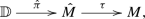
Using the universal cover ${\tilde{\pi }}: \mathbb {D}\rightarrow M$ of M we will also consider the immersion ${\tilde{f}}_M = f_M \circ {\tilde{\pi }}$ and write ${\tilde{{\mathfrak {f}}}}_M = {\mathfrak {f}}:\mathbb {D}\rightarrow S^5$.

We consider next the following diagram.

Lemma 1.2

One can choose without loss of generality ${\mathfrak {f}}$ such that the diagram commutes.

Proof

We have chosen ${\mathfrak {f}}$ such that the diagram

commutes, i.e., $\pi \circ {\mathfrak {f}}= {\tilde{f}}_M$. We also have the relations $f_M = \pi \circ {\mathfrak {f}}_M$ and ${\tilde{f}}_M = f_M \circ {\tilde{\pi }}$ and write ${\tilde{{\mathfrak {f}}}}_M = {\mathfrak {f}}:\mathbb {D}\rightarrow S^5$.

It suffices to prove that the diagram

commutes. We observe $\pi \circ {\mathfrak {f}}_M \circ {\tilde{\pi }} = f_M \circ {\tilde{\pi }} = {\tilde{{\mathfrak {f}}}}_M = \pi \circ {\mathfrak {f}}$. Therefore there exists a scalar function h with values in $S^1$ such that ${\mathfrak {f}}_M \circ {\tilde{\pi }} = h {\mathfrak {f}}$ holds. Thus by replacing ${\mathfrak {f}}$ by $h{\mathfrak {f}}$ we obtain the claim. $\square$

In the rest of the paper we will always assume that the diagrams just considered all commute. Also note that we have adjusted our notation so that objects defined on $\mathbb {D}$ usually have neither a $\tilde{.}$ nor the subscript M.

We want to define a (moving) frame for $f_M$ and will build it by using the lift ${\mathfrak {f}}:\mathbb {D}\rightarrow S^5$.

On $\mathbb {D}$ we will use the complex coordinates $z= x+ i y$ and ${{\bar{z}}} = x- i y$, respectively. In the following, the subscripts z and ${{\bar{z}}}$ denote the derivatives with respect to z and ${{\bar{z}}}$, respectively, defined via the Cauchy-Riemann operators

$$\begin{aligned} \partial _z := \frac{1}{2}\left( \frac{\partial }{\partial x} - i \frac{\partial }{\partial y}\right) , \quad \partial _{{{\bar{z}}}} := \frac{1}{2}\left( \frac{\partial }{\partial x} + i \frac{\partial }{\partial y}\right) . \end{aligned}$$

Thus we obtain, e.g.,

$$\begin{aligned} {\mathfrak {f}}_z = \partial _z {\mathfrak {f}}:= \frac{1}{2}\left( \frac{\partial {\mathfrak {f}}}{\partial x} - i \frac{\partial {\mathfrak {f}}}{\partial y}\right) , \quad {\mathfrak {f}}_{{{\bar{z}}}} = \partial _{{{\bar{z}}}} {\mathfrak {f}}:= \frac{1}{2}\left( \frac{\partial {\mathfrak {f}}}{\partial x} + i \frac{\partial {\mathfrak {f}}}{\partial y}\right) . \end{aligned}$$

The following definition is crucial for this paper

$$\begin{aligned} \xi := {\mathfrak {f}}_z - ({\mathfrak {f}}_z\cdot {\bar{{\mathfrak {f}}}}) {\mathfrak {f}}\quad \text{ and } \quad \eta := {\mathfrak {f}}_{{{\bar{z}}}} - ({\mathfrak {f}}_{{{\bar{z}}}}\cdot {\bar{{\mathfrak {f}}}}) {\mathfrak {f}}. \end{aligned}$$

(1.4)

After substitution into (1.2) the fact that the metric g is conformal gives

$$\begin{aligned}&\xi \cdot {{\bar{\eta }}} = \xi \cdot {{\bar{{\mathfrak {f}}}}} = \eta \cdot {{\bar{{\mathfrak {f}}}}} = 0, \end{aligned}$$

(1.5)

$$\begin{aligned}&e^{- \omega } \xi \cdot {{\bar{\xi }}} + e^{-\omega } \eta \cdot {{\bar{\eta }}} := a + b = 2, \end{aligned}$$

(1.6)

where we define

$$\begin{aligned} a :=e^{-\omega } \xi \cdot {{\bar{\xi }}} \quad \text{ and } \quad b := e^{-\omega }\eta \cdot {{\bar{\eta }}} . \end{aligned}$$

(1.7)

Writing temporarily $\xi = \xi [{\mathfrak {f}}]$ and analogously for $\eta$ it is easy to check that $\xi [ h{\mathfrak {f}}]= h \xi [{\mathfrak {f}}]$ and $\eta [h{\mathfrak {f}}] = h\eta [{\mathfrak {f}}]$ hold for all functions $h:\mathbb {D}\rightarrow S^1$. Therefore a and b are independent of the choices of the local lift ${\mathfrak {f}}$ and the complex coordinate z. Since $0 \le a,b \le 2$, we can define globally an invariant function $\theta : \mathbb {D}\rightarrow [0, \pi ]$ by

$$\begin{aligned} \theta := 2 \arccos \left( \sqrt{ \frac{a}{2}} \right) . \end{aligned}$$

(1.8)

It is easy to verify that the invariant $\theta$ defined above is exactly the Kähler angle of f, see for example [18]. In particular, $a = b$ is equivalent to f being Lagrangian. In this case $a = b = 1$.

Definition 1

A point $p \in \mathbb {D}$ is called holomorphic (anti-holomorphic or real respectively) for $f: \mathbb {D}\rightarrow \mathbb {C}P^2$ if $\theta (p) = 0$ ($\pi$ or $\frac{\pi }{2}$ respectively). A point is called a complex point of f, if it is holomorphic or anti-holomorphic.

Note that p is a complex point of f if and only if $a=0$ or $a = 2$. As a consequence, $\xi =0$ or $\eta =0$, respectively.

In order to be able to describe all immersions into $\mathbb {C}P^2$ without complex points we introduce two more invariants:

$$\begin{aligned} \Phi&:= e^{-\omega } \xi _{{{\bar{z}}}} \cdot {{\bar{\eta }}} dz := \phi dz, \end{aligned}$$

(1.9)

$$\begin{aligned} \Psi&:= \xi _{z} \cdot {{\bar{\eta }}} dz^3 := \psi dz^3. \end{aligned}$$

(1.10)

Using (1.5) one can easily check that $\Phi$ and $\Psi$ are independent of the choices of a lift ${\mathfrak {f}}$ of f and the complex coordinate z of $\mathbb {D}$ and thus are globally defined on the Riemann surface $\mathbb {D}$.

Moreover, if f is transformed by an isometry $T \in \mathrm{SU}_{3}$ to Tf, then $\xi$ and $\eta$ are transformed by T to $T\xi$ and $T\eta$ respectively. From the definitions it follows that $\Phi$ and $\Psi$ are $\mathrm{SU}_{3}$-invariant.

We call $\Psi$ the cubic Hopf differential and $\Xi = i(\Phi - {{\bar{\Phi }}})$ the mean curvature form. (Note, some authors call $\Phi$ the mean curvature form.)

Remark 1.3

The definitions of $\Phi$ and $\Psi$ show that the complex points of f are zeros of $\Phi$ and $\Psi$.

2.4 The moving frame equations for surfaces without complex points

$f:\mathbb {D}\rightarrow \mathbb {C}P^2$ be a contractible surface without complex points and let ${\mathfrak {f}}: \mathbb {D}\rightarrow S^5$ be a lift of f. We define $\xi$ and $\eta$ by (1.4). Then at each point of $\mathbb {D}$ we obtain a basis of $\mathbb {C}^3$ given by $\{\xi , \eta , {\mathfrak {f}}\}$.

We combine these vectors to form a matrix

$$\begin{aligned} \tilde{{\mathcal {F}}} = ( \xi , \eta ,{\mathfrak {f}}). \end{aligned}$$

Due to (1.5), (1.6) and the fact that ${\mathfrak {f}}\cdot {{\bar{{\mathfrak {f}}}}} = 1$ holds, this matrix satisfies the two equations

$$\begin{aligned} \tilde{{\mathcal {F}}}_z = \tilde{{\mathcal {F}}} \tilde{{\mathcal {U}}}, \quad \tilde{{\mathcal {F}}}_{{{\bar{z}}}} = \tilde{{\mathcal {F}}} \tilde{{\mathcal {V}}}, \end{aligned}$$

where

$$\begin{aligned} \tilde{{{\mathcal {U}}}}&= \begin{pmatrix} a_z/a + \omega _z + \rho + a^{-1} \phi &{} -a^{-1} {\bar{\phi }} &{} 1\\ b^{-1} e^{-\omega } \psi &{} \rho + b^{-1} \phi &{} 0\\ 0 &{} -be^\omega &{} \rho \end{pmatrix}, \;\;\\ \tilde{{{\mathcal {V}}}}&= \begin{pmatrix} - {{\bar{\rho }}} - a ^{-1} {{\bar{\phi }}} &{} -a^{-1} e^{-\omega } {{\bar{\psi }}} &{} 0 \\ b^{-1} \phi &{} b_{{{\bar{z}}}} /b + \omega _{{{\bar{z}}}} - {{\bar{\rho }}} -b^{-1} {\bar{\phi }}&{} 1\\ - a e^\omega &{} 0 &{} - {{\bar{\rho }}} \end{pmatrix}, \end{aligned}$$

and where we have abbreviated

$$\begin{aligned} \rho = {\mathfrak {f}}_z \cdot {{\bar{{\mathfrak {f}}}}}. \end{aligned}$$

(1.11)

Note, if we can choose ${\mathfrak {f}}$ as a horizontal lift, i.e., satisfying $d{\mathfrak {f}}\cdot {\bar{{\mathfrak {f}}}} = 0$, then $\rho = 0$.

The integrability condition

$$\begin{aligned} \tilde{{{\mathcal {U}}}}_{{{\bar{z}}}} - \tilde{{{\mathcal {V}}}}_z = [ \tilde{{{\mathcal {U}}}}, \tilde{{{\mathcal {V}}}}] \end{aligned}$$

splits into the following four scalar conditions

$$\begin{aligned}&\rho _{{\bar{z}}} + {{\bar{\rho }}}_z = (a-b) e^\omega , \end{aligned}$$

(1.12)

$$\begin{aligned}&(\log a)_{z {\bar{z}}} + \omega _{z {\bar{z}}} = (b-2a) e^\omega - (a^{-1} \phi )_{{\bar{z}}} - (a^{-1} {\bar{\phi }})_{z} - (ab)^{-1}|\phi |^2 +(ab)^{-1} e^{-2\omega }|\psi |^2 , \end{aligned}$$

(1.13)

$$\begin{aligned}&\psi _{{{\bar{z}}}} + (a^{-1} - b^{-1} ) {\bar{\phi }} \psi + (a^{-1} - b^{-1} ) e^\omega \phi ^2 = e^\omega (\phi _z - \omega _z \phi ) - e^\omega \phi (\log (ab))_z, \end{aligned}$$

(1.14)

$$\begin{aligned}&(\log b)_{z {\bar{z}}} + \omega _{z {\bar{z}}} = (a-2b) e^\omega + (b^{-1} \phi )_{{\bar{z}}} + (b^{-1} {\bar{\phi }})_{z} - (ab)^{-1}|\phi |^2 + (ab)^{-1} e^{-2\omega }|\psi |^2. \end{aligned}$$

(1.15)

We note that (1.12) is not essential. By using the Dolbeault Lemma, see [10, Theorem 13.2], we obtain

Proposition 1.4

One can choose without loss of generality ${\mathfrak {f}}$ such that $\rho$ satisfies

$$\begin{aligned} \partial _{{\bar{z}}} \rho = \frac{1}{2} (a-b) e^\omega . \end{aligned}$$

(1.16)

In this case we write $\rho _0$ instead of $\rho$.

Proof

Define $\rho _0$ as above. Then (1.12) is equivalent to

$$\begin{aligned} (\rho - \rho _0)_{{\bar{z}}} + \overline{ (\rho - \rho _0)_{ {{\bar{z}}} } } = 0. \end{aligned}$$

(1.17)

Moreover, $\Omega = i \{ (\rho - \rho _0)dz - \overline{(\rho - \rho _0)}d{{\bar{z}}} \}$ is a closed real 1-form. Let $\delta : \mathbb {D}\rightarrow \mathbb {R}$ denote a solution to $d \delta = \Omega .$ Then the new lift ${\tilde{{\mathfrak {f}}}} = e^{i \delta } {\mathfrak {f}}$ satisfies the compatibility conditions above with ${\tilde{\rho }} = \rho _0$. $\square$

Remark 1.5

• 1. The result above hinges heavily on the fact, that multiplication of ${\mathfrak {f}}$ by a scalar function with values in $S^1$ does not change $a, b, \omega , \phi$ and $\psi$, as was pointed out in a previous subsection.

• 2. But we will also need that the diagrams in Sect. 1.3 all commute. To maintain this fact we will also need to adjust ${\mathfrak {f}}_M$ by the same factor we have used for ${\mathfrak {f}}$.

For later use it will be convenient to bring the matrices $\tilde{{\mathcal {U}}}$ and $\tilde{{\mathcal {V}}}$ into a more symmetric form.

For this purpose we consider

$$\begin{aligned} {\mathcal {F}} = \tilde{{\mathcal {F}}} {\mathcal {R}}, \end{aligned}$$

where ${\mathcal {R}}$ denotes the diagonal matrix

$$\begin{aligned} {\mathcal {R}} = {\text {diag}}\left( -ie^{-\frac{\omega }{2}} \sqrt{a}^{-1}, -ie^{-\frac{\omega }{2}} \sqrt{b}^{-1},1\right) . \end{aligned}$$

Then we obtain

$$\begin{aligned} {\mathcal {F}}^{-1} d {\mathcal {F}} = {\mathcal {U}} dz + {\mathcal {V}} d {{\bar{z}}}, \end{aligned}$$

where

$$\begin{aligned} {{\mathcal {U}}}= & {} \begin{pmatrix} \frac{1}{2} \frac{a_z}{a} + \frac{1}{2} \omega _z + \rho + a^{-1} \phi &{} -\sqrt{ab}^{-1}{\bar{\phi }} &{} i\sqrt{a} e^{\frac{\omega }{2}}\\ \sqrt{ab}^{-1} e^{-\omega } \psi &{} - \frac{1}{2} \frac{b_z}{b} - \frac{1}{2} \omega _z +\rho + b^{-1} \phi &{} 0\\ 0 &{} i\sqrt{b}e^{ \frac{\omega }{2} }&{} \rho \end{pmatrix}, \end{aligned}$$

(1.18)

$$\begin{aligned} {{\mathcal {V}}}= & {} \begin{pmatrix} - \frac{1}{2} \frac{a_{{{\bar{z}}}}}{a} - \frac{1}{2} \omega _{{{\bar{z}}}} -{\bar{\rho }} - a^{-1} {\bar{\phi }} &{} -\sqrt{ab}^{-1} e^{-\omega } {\bar{\psi }} &{} 0 \\ \sqrt{ab}^{-1} \phi &{} \frac{1}{2} \frac{b_{{\bar{z}}}}{b} + \frac{1}{2} \omega _{{\bar{z}}} -{\bar{\rho }} - b^{-1} {\bar{\phi }}&{} i \sqrt{b} e^{\frac{\omega }{2} } \\ i\sqrt{a} e^{\frac{\omega }{2} } &{} 0 &{} - {{\bar{\rho }}} \end{pmatrix}. \end{aligned}$$

(1.19)

Several remarks are in place:

• 1. $\tilde{{\mathcal {F}}}$ and ${\mathcal {F}} = \tilde{{\mathcal {F}}} {\mathcal {R}}$ have the same last column. As a consequence ${\mathfrak {f}}= \tilde{{\mathcal {F}}} e_3 = {\mathcal {F}} e_3$. Hence a local lift of some immersion f without complex points can be retrieved from both frames.

• 2. ${\mathcal {V}} = - \bar{{\mathcal {U}}}^T$.

• 3. ${\text {trace}}({\mathcal {U}} )= (a^{-1} + b^{-1}) \phi + 3 \rho + \frac{1}{2} (\frac{a_z}{a} -\frac{b_z}{b} )$.

• 4. ${\text {trace}}({\mathcal {V}} ) = - \overline{{\text {trace}}({\mathcal {U}} )}$.

• 5. ${\mathcal {F}}^{-1} d {\mathcal {F}} = {\mathcal {U}} dz + {\mathcal {V}} d {{\bar{z}}}$ is skew-hermitian.

• 6. If the initial condition for the solution to the equation ${\mathcal {F}}^{-1} d {\mathcal {F}} = {\mathcal {U}} dz + {\mathcal {V}} d {{\bar{z}}}$ is in $\mathrm{U}_{3}$, then the whole solution ${\mathcal {F}}$ is in $\mathrm{U}_{3}$. In particular, in this case $\det ({\mathcal {F}}) \in S^1.$

• 7. Sometimes we will need to know from which ${\mathfrak {f}}$ the frame ${\mathcal {F}}$ has been constructed. In such a case we write ${\mathcal {F}} = {\mathcal {F}} ({\mathfrak {f}})$.

With these pieces of information we obtain

Theorem 1.6

(Fundamental Theorem of liftable surfaces in $\mathbb {C}P^2$ without complex points, [11])

• 1. Let $f_M:M \rightarrow \mathbb {C}P^2$ be a liftable immersion without complex points and lift ${\mathfrak {f}}_M: M \rightarrow S^5$. Let $g = 2 e^\omega dz d{\bar{z}}$ denote the induced metric, $\theta : \mathbb {D}\rightarrow (0, \pi )$ the Kähler angle, $\Psi$ the cubic form, $\Phi$ the mean curvature form (all defined from ${\mathfrak {f}}$ as in Sect. 1.3). Set $a=2\cos \frac{\theta }{2}$, $b=2\sin \frac{\theta }{2}$ and $\rho =\rho _0$ is defined by (1.11). Then the conditions (1.12), (1.13), (1.14) and (1.15) are satisfied.

• 2. Conversely, let $g = 2 e^\omega dz d{\bar{z}}$ be a Riemannian metric on the simply connected Riemann surface $\mathbb {D}$. Let $\theta : \mathbb {D}\rightarrow (0,\pi )$ be a real valued function and $\Phi$ and $\Psi$ a (1, 0)-form and a (3, 0)-form on $\mathbb {D}$ respectively. Set $a=2\cos \frac{\theta }{2}$, $b=2\sin \frac{\theta }{2}$ and $\rho =\rho _0$ is given in Proposition 1.4. If these data satisfy the conditions (1.12), (1.13), (1.14) and (1.15), then there exists an immersion $f:\mathbb {D}\rightarrow \mathbb {C}P^2$ without complex points such that the given data have the meaning for f as stated in (1). In particular, in this case the given data are the corresponding invariants for some lift ${\mathfrak {f}}: \mathbb {D}\rightarrow S^5$ of f.

  Moreover, if ${\mathfrak {f}}$ descends to a map ${\hat{{\mathfrak {f}}}}: {\hat{M}} \rightarrow S^5$ for some Riemann surface ${\hat{M}}$, then $\pi \circ {\hat{{\mathfrak {f}}}} : {\hat{M}} \rightarrow \mathbb {C}P^2$ is a liftable immersion without complex points from ${\hat{M}}$ to $\mathbb {C}P^2$.

• 3. If two isometric surfaces $f: \mathbb {D}\rightarrow \mathbb {C}P^2$ and ${\hat{f}} : {\hat{\mathbb {D}}}\rightarrow \mathbb {C}P^2$ without complex points have the same forms $\Phi$ and $\Psi$ and the same Kähler function $\theta$, i.e., if there exists some diffeomorphism $\kappa : \mathbb {D}\rightarrow {\hat{\mathbb {D}}}$ such that $g = \kappa ^* {\hat{g}}$, $\theta = {\hat{\theta }} \circ \kappa$, $\Phi = \kappa ^* {{\hat{\Phi }}}$ and $\Psi = \kappa ^*{{{\hat{\Psi }}}}$, then there exists an isometry $T \in \mathrm{SU}_{3}$ such that $f = T \circ {\hat{f}} \circ \kappa$.

The following result will be particularly convenient.

Theorem 1.7

Let $f_M:M \rightarrow \mathbb {C}P^2$ be a liftable immersion without complex points. Then one can choose, without loss of generality, a lift ${\mathfrak {f}}_M: M \rightarrow S^5$ of f such that the corresponding frame ${\mathcal {F}}$ has determinant 1. Such lift is called a special lift for $f_M$.

Proof

First we note that ${\mathcal {F}}$ is unitary and thus has determinant $\delta$ in $S^1$. Since ${\mathcal {F}}$ is defined on $\mathbb {D}$, we can take a cubic root of $\delta$. Let $h\in S^1$ denote the inverse of this cubic root. Then the property $\xi [ h{\mathfrak {f}}]= h \xi [{\mathfrak {f}}]$ and $\eta [h{\mathfrak {f}}] = h\eta [{\mathfrak {f}}]$ for all functions $h:\mathbb {D}\rightarrow S^1$ implies the claim, where we also need to adjust ${\mathfrak {f}}_M$ as before. $\square$

Corollary 1.8

Under the assumptions above one can specialize the lift ${\mathfrak {f}}_M$ in two ways (by multiplication by a function with values in $S^1$) so that one can assume that $\rho = \rho _0$ holds, or so that ${\mathcal {F}} \in \mathrm{SU}_{3}$ holds.

From here on we will always assume that ${\mathcal {F}} \in \mathrm{SU}_{3}$. It is important to note that now $\rho$ can not be assumed to have the special form $\rho _0$.

Corollary 1.9

Under the assumptions above the trace of the Maurer-Cartan form of ${\mathcal {F}}$ vanishes identically.

In the case of minimal Lagrangian surfaces, $a=b=1$ and $\Phi \equiv 0$, thus one can have a horizontal lift ${\mathfrak {f}}$, i.e., $\rho =0$ and the trace of the Maurer–Cartan form of ${\mathcal {F}}$ vanishes automatically.

3 Algebraic digression

In this section we discuss briefly the algebraic setting which will be used in the following sections.

3.1 The automorphism $\sigma$

We consider the order 6 automorphism $\sigma$ of the Lie algebra ${\mathfrak {g}} = {\mathfrak {sl}}_3{\mathbb {C}}$, given by

$$\begin{aligned} \sigma ( X) = - P X^T P, \quad \text{ where } \quad P = \begin{pmatrix} 0&{}\quad \epsilon ^2 &{}\quad 0\\ \epsilon ^4&{}\quad 0 &{}\quad 0\\ 0&{}\quad 0&{}\quad 1\\ \end{pmatrix} \end{aligned}$$

(2.1)

with $\epsilon = e^{\frac{ i\pi }{3}}$. We also consider the connected Lie group $G = {\mathrm{SL}}_3{\mathbb {C}}$ and the automorphism $\sigma ^G$ of order 6

$$\begin{aligned} \sigma ^G(g) = P (g^{T})^{-1}P. \end{aligned}$$

(2.2)

Then $\sigma$ is the differential of $\sigma ^G$ and we will use from now on the same notation for both homomorphisms. By abuse of notation we will also write $\sigma ^G$ by $\sigma$. We would like to point out that $\sigma$ is an outer automorphism of ${\mathfrak {g}}$.

By a simple computation we obtain

$$\begin{aligned} \sigma ^2 (X) = P_2 X P_2^{-1},\quad \text{ with } \quad P_2 = {\text {diag}}( \epsilon ^4, \epsilon ^2, 1). \end{aligned}$$

(2.3)

The formula on the group level is the same. We would like to point out that $\sigma ^2$ is an inner automorphism.

Finally we derive

$$\begin{aligned} \sigma ^3 ( X) = -P_3 X^T P_3, \quad \text{ with } \quad P _3= \begin{pmatrix} 0&{}\quad 1 &{}\quad 0\\ 1&{}\quad 0 &{}\quad 0\\ 0&{}\quad 0&{}\quad 1\\ \end{pmatrix}. \end{aligned}$$

(2.4)

We would like to point out that $\sigma ^3$ is an outer automorphism of ${\mathfrak {g}}$. In the context of certain surface classes we will discuss the automorphisms $\sigma$, $\sigma ^2$ and $\sigma ^3$ of ${\mathfrak {g}}$.

Since, the eigenspaces of the various powers of $\sigma$ all can be derived from the eigenspaces of $\sigma$, we discuss this case first. Explicitly the eigenspaces ${\mathfrak {g}}_k$ of $\sigma$ with respect to the eigenvalue $\epsilon ^k$ in ${\mathfrak {sl}}_3{\mathbb {C}}$ are given as follows

$$\begin{aligned} {\mathfrak {g}}_0&\quad =\left\{ \begin{pmatrix} a &{}\quad &{}\quad \\ &{}\quad -a &{}\quad \\ &{}\quad &{}\quad 0 \\ \end{pmatrix} \mid a\in \mathbb {C}\right\} , \quad {\mathfrak {g}}_1=\left\{ \begin{pmatrix} 0 &{}\quad b &{}\quad 0 \\ 0 &{}\quad 0 &{}\quad a \\ a &{}\quad 0 &{}\quad 0 \\ \end{pmatrix}\mid a,b\in \mathbb {C}\right\} , \\ {\mathfrak {g}}_2&\quad =\left\{ \begin{pmatrix} 0 &{}\quad 0&{}\quad a \\ 0&{}\quad 0 &{}\quad 0 \\ 0&{}\quad -a &{}\quad 0 \\ \end{pmatrix} \mid a\in \mathbb {C}\right\} , \quad {\mathfrak {g}}_3=\left\{ \begin{pmatrix} a &{}\quad &{}\quad \\ &{}\quad a &{}\quad \\ &{}\quad &{}\quad -2a \\ \end{pmatrix} \mid a\in \mathbb {C}\right\} ,\\ {\mathfrak {g}}_4&\quad =\left\{ \begin{pmatrix} 0 &{}\quad 0 &{}\quad 0 \\ 0&{}\quad 0 &{}\quad a \\ -a &{}\quad 0 &{}\quad 0 \\ \end{pmatrix} \mid a\in \mathbb {C}\right\} , \quad {\mathfrak {g}}_5=\left\{ \begin{pmatrix} 0 &{}\quad 0 &{}\quad a \\ b &{}\quad 0 &{}\quad 0 \\ 0 &{}\quad a &{}\quad 0 \\ \end{pmatrix} \mid a, b\in \mathbb {C}\right\} . \end{aligned}$$

The eigenspaces of $\sigma ^2$ are

• ${\mathfrak {g}}_1 + {\mathfrak {g}}_4$ for the eigenvalue $\epsilon ^2$,

• ${\mathfrak {g}}_2 + {\mathfrak {g}}_5$ for the eigenvalue $\epsilon ^4$,

• ${\mathfrak {g}}_3 + {\mathfrak {g}}_0$ for the eigenvalue 1.

The eigenspaces for $\sigma ^3$ are

• ${\mathfrak {g}}_4 + {\mathfrak {g}}_2 + {\mathfrak {g}}_0$ for the eigenvalue 1,

• ${\mathfrak {g}}_1 + {\mathfrak {g}}_3 + {\mathfrak {g}}_5$ for the eigenvalue $\epsilon ^3 = -1$.

3.2 The real form involution $\tau$

The real form ${{\mathfrak {g}}}^{\mathbb {R}}={\mathfrak {su}}_3$ of ${{\mathfrak {g}}} = {\mathfrak {sl}}_3{\mathbb {C}}$ is given by the anti-linear involution

$$\begin{aligned} \tau (X) = - {{\bar{X}}}^T, \quad X \in {\mathfrak {sl}}_3{\mathbb {C}}. \end{aligned}$$

We also consider the anti-linear involution $\tau ^G$ on $G = {\mathrm{SL}}_3{\mathbb {C}}$

$$\begin{aligned} \tau ^G (g) = ({{\bar{g}}}^T)^{-1}, \quad g \in {\mathrm{SL}}_3{\mathbb {C}}. \end{aligned}$$

(2.5)

By abuse of notation we will also write $\tau ^{G}$ by $\tau$. Then a direct computation shows that $\sigma$ in (2.1) and $\tau$ commute, i.e., $\tau \circ \sigma = \sigma \circ \tau$, thus $\tau$ and the eigenspaces of $\sigma$ have the relation

$$\begin{aligned} \tau ({{\mathfrak {g}}}_j) = {{\mathfrak {g}}}_{-j}, \quad j=0, 1, \dots , 5. \end{aligned}$$

(2.6)

In particular ${{\mathfrak {g}}}_0$ and ${{\mathfrak {g}}}_0 \oplus {{\mathfrak {g}}}_3$ are subalgebras of ${\mathfrak {su}}_3$ with the obvious complexifications.

3.3 k-symmetric spaces

As we discussed in Sect. 2.2, $\sigma$ and $\tau$ commute, and thus we arrive at a definition of k-symmetric spaces, as it will be used in our paper.

Definition 2

Let $G^{\mathbb {R}}/G^{\mathbb {R}}_0$ be a real homogeneous space such that $G^{\mathbb {R}}$ is a real form of a complex Lie group G given by a real form involution $\tau$, that is, $G^{\mathbb {R}} = {\text {Fix}}(G, \tau )$. Moreover, let $\sigma$ be an order $k \;(k\ge 2)$ automorphism of G,  leaving $G^{\mathbb {R}}$ invariant and commuting with $\tau$. Then $G^{\mathbb {R}}/G^{\mathbb {R}}_0$ is called a k-symmetric space if the following condition is satisfied

$$\begin{aligned} {\text {Fix}}(G^{\mathbb {R}},\sigma )^\circ \subset G^{\mathbb {R}}_0 \subset {\text {Fix}}(G^{\mathbb {R}}, \sigma ), \end{aligned}$$

(2.7)

where ${\text {Fix}}(G^{\mathbb {R}}, \sigma )^\circ$ denotes the identity component of ${\text {Fix}}(G^{\mathbb {R}}, \sigma )$.

3.4 Primitive maps and the loop group formalism

In the last subsection we have discussed complex Lie algebras and Lie groups. For the applications to geometry we will need to work with real Lie groups.

Thus we consider a complex Lie group as before and let $\tau$ denote an anti-holomorphic involution of G. Then we put

$$\begin{aligned} G^\mathbb {R}= {\text {Fix}}(G,\tau ). \end{aligned}$$

Similarly we define ${\text {Lie}}G^\mathbb {R}= {\mathfrak {g}}^\mathbb {R}.$

Definition 3

Let $\kappa$ be any automorphism of ${\mathfrak {g}}$ of finite order $k > 2$. Let ${\mathfrak {g}}_m$ denote the eigenspaces of $\kappa$, where we choose $m \in \mathbb {Z}$ and actually work with $m \mod k$. Let ${\mathcal {F}} : \mathbb {D}\rightarrow G$ be a smooth map. Then ${\mathcal {F}}$ will be called primitive relative to $\kappa$ if

$$\begin{aligned} {\mathcal {F}}^{-1} d{\mathcal {F}} = \alpha _{-1} dz + \alpha _0^{\prime } dz+\alpha _0^{\prime \prime } d{\bar{z}}+ \alpha _1 d{\bar{z}} \in {\mathfrak {g}}_{-1} + {\mathfrak {g}}_0 + {\mathfrak {g}}_1, \end{aligned}$$

where $\alpha _m$, $\alpha _0^{\prime }$ and $\alpha _0^{\prime \prime }$ take values in an eigenspace ${\mathfrak {g}}_m$ of $\kappa$.

By abuse of notation we will also write $\alpha _0 = \alpha _0^\prime dz + \alpha _0^{\prime \prime }d {\bar{z}}$.

Lemma 2.1

Let ${\mathcal {F}}$ be primitive relative to $\kappa$ and let us write ${\mathcal {F}}^{-1} d{\mathcal {F}} = \alpha _{-1} dz+ \alpha _0 + \alpha _1 d {\bar{z}}$. Then $\lambda ^{-1} \alpha _{-1} dz+ \alpha _0 + \lambda \alpha _1d {\bar{z}}$ is integrable for all $\lambda \in \mathbb {C}^*$.

Proof

Together with a straightforward computation one needs to use that because of $k>2$ the sum ${\mathfrak {g}}_{-1} + {\mathfrak {g}}_0 + {\mathfrak {g}}_1$ of eigenspaces is direct. $\square$

The importance of this observation has been elaborated on and explained in [2, Section 3.2] and [1].

Theorem 2.2

[1, 2] Let G be a complex Lie group, $\sigma$ an automorphism of G of finite order $k \ge 2$ and $\tau$ an anti-holomorphic involution of G which commutes with $\sigma$. Let $G^\mathbb {R}_0$ be any Lie subgroup of $G^\mathbb {R}$ satisfying ${\text {Fix}}(G^\mathbb {R}, \sigma )^{\circ } \subset {G^\mathbb {R}_0} \subset {\text {Fix}}(G^\mathbb {R}, \sigma )$. Then we consider the k-symmetric space $G^\mathbb {R}/ {G^\mathbb {R}_0}$ together with the (pseudo-)Riemannian structure induced by some bi-invariant (pseudo-)Riemannian structure on $G^\mathbb {R}$. Let $h:\mathbb {D}\rightarrow G^\mathbb {R}/ {G^\mathbb {R}_0}$ be a smooth map and ${\mathcal {F}} : \mathbb {D}\rightarrow G^\mathbb {R}$ a frame for h, i.e., $h = \pi \circ {\mathcal {F}}$, where $\pi : G^\mathbb {R}\rightarrow G^{\mathbb {R}}/{G^\mathbb {R}_0}$ denotes the canonical projection.

Then the following statements hold:

• 1. If $k=2$, then h is harmonic if and only if $\lambda ^{-1} \alpha _{-1} dz+ \alpha _0 + \lambda \alpha _1 d{\bar{z}}$ is integrable for all $\lambda \in \mathbb {C}^*$.

• 2. If $k>2$, then h is harmonic if ${\mathcal {F}}$ is primitive relative to $\sigma$.

From the above theorem, we have the following definition.

Definition 4

Retain the notation in Theorem 2.2.

• 1. The frame ${{\mathcal {F}}}$ is called primitive harmonic, if ${\mathcal {F}}^{-1} d{\mathcal {F}} = \alpha _{-1}dz + \alpha _0 + \alpha _1 d {\bar{z}}$ such that $\lambda ^{-1} \alpha _{-1} dz+ \alpha _0 + \lambda \alpha _1 d{\bar{z}}$ is integrable for all $\lambda \in \mathbb {C}^*$.

• 2. The map h is called primitive harmonic map, if the frame ${{\mathcal {F}}}$ is primitive harmonic.

This admits a direct application of the loop group method (see [8] for the basic formalism, presented in loc.cit. for compact groups.)

The first step here is to integrate

$$\begin{aligned} {\mathcal {F}}_{\lambda }^{-1} d{\mathcal {F}}_{\lambda } = \lambda ^{-1} \alpha _{-1} dz+ \alpha _0 + \lambda \alpha _1d {\bar{z}}. \end{aligned}$$

Since $\tau$ maps ${\mathfrak {g}}_m$ to ${\mathfrak {g}}_{-m}$, we can assume that ${\mathcal {F}}_\lambda$ is contained in $G^\mathbb {R}$ for all $\lambda \in S^1$. Note that we will write ${\mathcal {F}}(z,\lambda )$ or ${\mathcal {F}}_\lambda (z)$, whatever is most convenient. We will usually also assume ${\mathcal {F}}(z_0,\lambda ) = I$ for a once and for all fixed base point $z_0$.

Then it follows from the above that also $h_\lambda = {\mathcal {F}}_\lambda \mod G^\mathbb {R}_0$ is a primitive harmonic map with frame ${\mathcal {F}}_\lambda$. Usually ${\mathcal {F}}_\lambda$ is called an extended frame for h.

The loop group method constructs in principle all these extended frames. For this one does not read ${\mathcal {F}}(z,\lambda )$ as a family of frames, parametrized by $\lambda$, but as a function of z into some loop group.

Here are the basic definitions:

• 1. $\Lambda G = \{ g: S^1 \rightarrow G \}.$ Considering G as a subgroup of some matrix algebra ${\text {Mat}} (n,\mathbb {C})$ we use the Wiener norm on $\Lambda {\text {Mat}} (n,\mathbb {C})$ and thus induce a Banach Lie group structure on $\Lambda G$.

• 2. $\Lambda ^+G = \left\{ g \in G\mid \begin{array}{l} g \text{ has } \text{ a } \text{ holomorphic } \text{ extension } \text{ to } \text{ the } \text{ open } \text{ unit } \text{ disk }\\ \text{ and } g^{-1} \text{ has } \text{ the } \text{ same } \text{ property } \end{array} \right\}$.

• 3. $\Lambda _*^+G = \{ g \in \Lambda ^+G \mid g(0) = I \}.$

• 4. $\Lambda ^-G = \left\{ g \in G \mid \begin{array}{l} g \text{ has } \text{ a } \text{ holomorphic } \text{ extension } \text{ to } \text{ the } \text{ open } \text{ upper } \text{ unit } \text{ disk } \text{ in } \mathbb {C}P^1 \\ \text{ and } g^{-1} \text{ has } \text{ the } \text{ same } \text{ property } \end{array} \right\} .$

• 5. $\Lambda _*^-G = \{ g \in \Lambda ^-G \mid g(\infty ) = I \}.$

• 6. $\Lambda G^\mathbb {R}= \{g \in \Lambda G\mid \tau (g(\lambda ) )= g(\lambda ) \text{ for } \text{ all } \quad \lambda \in S^1\}$.

Finally, we will actually always use twisted subgroups of the groups above. First we have

$$\begin{aligned} \Lambda G_{\sigma }= \left\{ g \in \Lambda G\mid \sigma ( g( \epsilon ^{- 1} \lambda )) = g(\lambda ) \text{ for } \text{ all } \lambda \in S^1 \right\} . \end{aligned}$$

The other twisted groups are defined analogously, like

$$\begin{aligned} \Lambda _*^+G _{\sigma } = \Lambda _*^+G \cap \Lambda G_{\sigma }. \end{aligned}$$

By the form of ${\mathcal {F}}_{\lambda }^{-1} d{\mathcal {F}}_{\lambda }$ we infer that all the loop matrices associated with geometric quantities are actually defined for all $\lambda \in \mathbb {C}^*$. However, geometric interpretations are usually only possible for $\lambda \in S^1$.

To understand the construction procedure mentioned above one considers next again h and ${\mathcal {F}}$ as above and decomposes

$$\begin{aligned} {\mathcal {F}}(z,\lambda ) = {\mathcal {C}}(z,\lambda ) \cdot {\mathcal {L}}_+(z,\lambda ), \end{aligned}$$

where ${\mathcal {C}}$ is holomorphic in $z \in \mathbb {D}$ and holomorphic in $\lambda \in \mathbb {C}^*$ and ${\mathcal {L}}_+(z,\lambda ) \in \Lambda ^+G _{\sigma }$.

Since $S^2$ does not occur in this paper as domain of a harmonic map, such a decomposition is always possible, and defines a holomorphic potential $\eta$ for h by the formula

$$\begin{aligned} \eta = {\mathcal {C}}^{-1} d{\mathcal {C}}. \end{aligned}$$

The potential $\eta$ takes the form

$$\begin{aligned} \eta = \lambda ^{-1} \eta _{-1}(z) dz + \lambda ^{0} \eta _{0}(z) dz +\lambda ^{1} \eta _{1}(z) dz +\lambda ^{2} \eta _{2}(z) dz + \cdots . \end{aligned}$$

(2.8)

We would like to emphasize:

• 1. All coefficient functions $\eta _j$ are holomorphic on $\mathbb {D}$.

• 2. All $\eta _j$ are contained in ${\mathfrak {g}}_{m(j)}$, where $m(j) = 0,1,2,\dots ,k-1$ and $m(j) \equiv j \mod k$.

This explains the procedure to obtain a holomorphic potential from a primitive harmonic map. The fortunate point is that this procedure can be reversed.

The following theorem is a straightforward generalization of a result of [8].

Theorem 2.3

(Loop group procedure, [8]) Let $G, \sigma$ and $\tau$ as above. Let $h:\mathbb {D}\rightarrow G^\mathbb {R}/ {G^\mathbb {R}_0}$ be a primitive harmonic map with extended frame ${\mathcal {F}}_\lambda$. Define ${\mathcal {C}}$ by ${\mathcal {F}}(z,\lambda ) = {\mathcal {C}}(z,\lambda ) \cdot {\mathcal {L}}_+(z,\lambda )$ and put $\eta = {\mathcal {C}}^{-1} d{\mathcal {C}}$. Then $\eta$ has the form stated in (2.8), the coefficient functions $\eta _j$ of $\eta$ are holomorphic on $\mathbb {D}$ and we have $\eta _j \in {\mathfrak {g}}_{m(j)}$ and $m(j) \equiv j \mod k$.

Conversely, consider any holomorphic 1-form $\xi$ satisfying the three conditions just listed for $\eta$. Then solve the ODE $d{\mathcal {C}} = {\mathcal {C}} \xi$ on $\mathbb {D}$ with ${\mathcal {C}} \in \Lambda G$. Next write ${\mathcal {C}} = {\mathcal {F}} _\lambda \cdot {\mathcal {V}}_+$ with ${\mathcal {F}}_\lambda \in \Lambda G^\mathbb {R}_{\sigma }$ and ${\mathcal {V}}_+ \in \Lambda ^+G _{\sigma }$. Then ${\mathcal {F}}_\lambda$ is the extended frame of the associated family of some primitive harmonic map $h : \mathbb {D}\rightarrow G^\mathbb {R}/ {G^\mathbb {R}_0}.$

3.5 Evaluation of the meaning of primitive harmonic maps relative to $\sigma$, $\sigma ^2$, and $\sigma ^3$

We start by evaluating what it means that a Maurer-Cartan form of some frame of some liftable immersion into $\mathbb {C}P^2$ without complex points is primitive relative to $\sigma$, $\sigma ^2$, or $\sigma ^3$ respectively.

We will use the notation introduced just above.

Theorem 2.4

Let $G = {\mathrm{SL}}_3{\mathbb {C}}$ and ${\mathfrak {g}} = {\mathfrak {sl}}_3{\mathbb {C}}$ its Lie algebra. Let $\tau$ denote the real form involution of G singling out $G^{\mathbb {R}}=\mathrm{SU}_{3}$ in G and let $\sigma = \sigma ^G$ be the automorphism of order 6 of G given by $\sigma (g) = P (g^{T})^{-1} P$ in (2.1). Assume moreover, that ${\mathfrak {f}}$ is the lift of a liftable immersion f into $\mathbb {C}P^2$ without complex points and with frame ${{\mathcal {F}}}$ in $G^{\mathbb {R}}$. Then the following statements hold:

• 1. ${{\mathcal {F}}}$ is primitive harmonic relative to $\sigma$ if and only if f is minimal Lagrangian in $\mathbb {C}P^2$.

• 2. ${{\mathcal {F}}}$ is primitive harmonic relative to $\sigma ^2$ if and only if f is minimal in $\mathbb {C}P^2$ without complex points.

• 3. ${{\mathcal {F}}}$ is primitive harmonic relative to $\sigma ^3$ if and only if either f is minimal Lagrangian or f is flat homogeneous in $\mathbb {C}P^2$.

Remark 2.5

From Theorem 2.4, in each case, we have a primitive harmonic map in $G^{\mathbb {R}}/G_0^{\mathbb {R}}$ relative to $\sigma$, $\sigma ^2$ and $\sigma ^3$, respectively. We will discuss these maps in Sect. 3 in detail.

Proof

Since our statement basically only uses local properties, we can assume without loss of generality that f and ${\mathfrak {f}}$ are defined on a contractible domain $\mathbb {D}$.

1. We consider the Maurer-Cartan form $\alpha$ of some frame of ${\mathfrak {f}}$. Then primitive harmonicity relative to $\sigma$ means that there is no component of $\alpha$ in the spaces ${\mathfrak {g}}_j$, $j = 2,3,4$. It is straightforward to see that this is equivalent to $\phi = 0$, $a=b (=1)$ and that the diagonal is in ${\mathfrak {g}}_0$. In particular $\rho = 0$ and the matrices (1.18) and (1.19) have exactly the form of the Maurer-Cartan form of a minimal Lagrangian immersion (including the case $\Psi = 0$).

2. We consider again the Maurer-Cartan form of ${\mathfrak {f}}$. Then primitive harmonicity relative to $\sigma ^2$ means that there is no component of ${\mathcal {U}}$ in the spaces ${\mathfrak {g}}_j$, $j = 1, 4$, and there is no component of ${\mathcal {V}}$ in the spaces ${\mathfrak {g}}_j$, $j = 2, 5$. These two conditions are equivalent to $\phi = 0$.

Thus the primitivity relative to $\sigma ^2$ is equivalent to f being minimal without complex points by Theorem 1.6.

3. In this case we need to consider ${{\mathcal {U}}} = {{{\mathcal {U}}}}_0 + \lambda {{\mathcal {U}}}_1$ for all $\lambda \in S^1$, where ${{\mathcal {U}}}_0$ takes values in the fixed point space of $\sigma ^3$ and ${{\mathcal {U}}}_1$ takes values in the eigenspace for the eigenvalue $-1$.

From section 2 we know that the eigenspaces for $\sigma ^3$ are ${\mathfrak {g}}_4 + {\mathfrak {g}}_2 + {\mathfrak {g}}_0$ for the eigenvalue 1 and ${\mathfrak {g}}_1 + {\mathfrak {g}}_3 + {\mathfrak {g}}_5$ for the eigenvalue $\epsilon ^3 = -1$. We thus consider a primitive 1-form ${\hat{\alpha }} = {\mathcal {U}} dz + {\mathcal {V}} d {{\bar{z}}}$, where ${\mathcal {U}}$ is of the form

$$\begin{aligned} {{\mathcal {U}}} = {{\mathcal {U}}}_0 + \lambda ^{-1} {{\mathcal {U}}}_1, \end{aligned}$$

where

$$\begin{aligned} {{\mathcal {U}}}_0&= \begin{pmatrix} u_{11} &{} 0 &{} \frac{i}{2} (\sqrt{a}- \sqrt{b}) e^{\frac{\omega }{2}}\\ 0 &{} -u_{11} &{} 0\\ 0 &{} - \frac{i}{2} (\sqrt{a}- \sqrt{b}) e^{\frac{\omega }{2}} &{} 0 \end{pmatrix}, \\ {{\mathcal {U}}}_1&= \begin{pmatrix} w &{} - \sqrt{ab}^{-1} \phi &{} \frac{i}{2} (\sqrt{a} + \sqrt{b}) e^{\frac{\omega }{2}}\\ \sqrt{ab}^{-1} e^{-\omega } \psi &{} w &{} 0\\ 0 &{} \frac{i}{2} (\sqrt{a} + \sqrt{b}) e^{\frac{\omega }{2}} &{} -2w \end{pmatrix}, \end{aligned}$$

and an analogous expression holds for ${\mathcal {V}} = -(\overline{{\mathcal {U}}})^T.$

We already know from the beginning of the proof that for $\lambda = 1$ the map ${\mathfrak {f}}$ comes from some immersion f into $\mathbb {C}P^2$ without complex points. It thus is of importance to observe that our 1-form $\alpha$ has the form stated in (1.18) and (1.19). As a consequence, we know the form of the diagonal entries of ${\mathcal {U}}$ and ${\mathcal {V}}$.

Next we evaluate the integrability condition $d \alpha + \frac{1}{2} [\alpha \wedge \alpha ] = 0$. Expanding in $\lambda$ it is easy to see that only the following two equations need to be evaluated:

• 1. $\partial _{{\bar{z}}} {\mathcal {U}}_1 = [ {\mathcal {U}}_1, {\mathcal {V}}_0]$,

• 2. $\partial _{{\bar{z}}} {\mathcal {U}}_0 - \partial _{z} {\mathcal {V}}_0 = [ {\mathcal {U}}_1 ,{\mathcal {V}}_1 ] + [ {\mathcal {U}}_0 , {\mathcal {V}}_0 ]$.

We look first at the first of these matrix equations and evaluate the (11)-entry and the (23)-entry. After a simple computation we obtain $\partial _{{\bar{z}}} w = -\frac{1}{4} (a-b) e^\omega$ and $-3 w \frac{i}{2} (\sqrt{a} - \sqrt{b}) e^{\frac{\omega }{2}} = 0$. Altogether we conclude that $a=b$ holds on $\mathbb {D}$. In particular we then also have $a=b=1$ and that w is holomorphic.

We can assume, since we have normalized our frames to have determinant 1, by using formula (3) after (1.19), that ${\text {trace}}({\mathcal {U}} )= (a^{-1} + b^{-1}) \phi + 3 \rho + \frac{1}{2} (\frac{a_z}{a} -\frac{b_z}{b} )= 0,$ holds. Thus we have $\rho = - \frac{2}{3} \phi = -2 w$. In particular, $\phi$ is holomorphic.

Evaluating the matrix equation (1) above further, we obtain from the matrix entry (13) the equation $\frac{\omega _z}{2} = u_{11}$. Now the equations for the matrix entries (12) and (21) imply $\partial _{{\bar{z}}}\phi = 2{\bar{u}}_{11} \phi$ and that $\psi$ is holomorphic respectively. As a result, $\phi = 0$ and the 1-form $\alpha$ is exactly the Maurer-Cartan form of the $\mathrm{SU}_{3}$-frame of a minimal Lagrangian immersion, or $\omega$, $\phi$ and $\psi$ are all constant with $\psi$ is non-vanishing, which gives a Lagrangian homogeneous surface. One can check easily that with these conditions the 1-form $\alpha$ actually is primitive relative to $\sigma ^3$. $\square$

In the sections above we had always assumed that we start from some liftable immersion into $\mathbb {C}P^2$ and consider the frame constructed at the beginning of this paper.

The next theorem is more general. As before we will use $e_3 = (0,0,1)^T$.

Theorem 2.6

Let ${\hat{{\mathfrak {f}}}} : \mathbb {D}\rightarrow S^5$ be a smooth map and $\hat{{\mathcal {F}}}:\mathbb {D}\rightarrow \mathrm{SU}_{3}$ a frame such that $\hat{{\mathcal {F}}}.e_3 = {{\hat{{\mathfrak {f}}}}}$. Moreover, we assume that the Maurer-Cartan form ${\hat{\alpha }}$ of $\hat{{\mathcal {F}}}$ has the general form, more precisely we thus consider a 1-form ${\hat{\alpha }} = \hat{ {\mathcal {U}}} dz + \hat{{\mathcal {V}}} d {{\bar{z}}}$, in $\Lambda {{\mathfrak {su}}}_3$, where

$$\begin{aligned} \hat{{{\mathcal {U}}}} = \begin{pmatrix} u_{11} + w &{} u_{12} &{} u_{13}\\ u_{21} &{} -u_{11} + w &{} 0\\ 0 &{} u_{32} &{} - 2 w \end{pmatrix}, \end{aligned}$$

and

$$\begin{aligned} \hat{{{\mathcal {V}}}} = \begin{pmatrix} -{\bar{u}}_{11} -{\bar{w}} &{} -{\bar{u}}_{21} &{} 0 \\ -{\bar{u}}_{12} &{} {\bar{u}}_{11} -{\bar{w}} &{}- {\bar{u}}_{32}\\ -{\bar{u}}_{13} &{} 0 &{} 2 {\bar{w}}\\ \end{pmatrix}. \end{aligned}$$

Furthermore, we assume that $u_{13}$ and $u_{23}$ never vanish. Then the following statements hold:

• 1. Each primitive harmonic $\hat{{\mathcal {F}}}$ relative to $\sigma$ can be derived from a minimal Lagrangian immersion in $\mathbb {C}P^2$.

• 2. Each primitive harmonic $\hat{{\mathcal {F}}}$ relative to $\sigma ^2$ can be derived from a minimal immersion in $\mathbb {C}P^2$ without complex points.

• 3. Each primitive harmonic $\hat{{\mathcal {F}}}$ relative to $\sigma ^3$ can be derived from a minimal Lagrangian immersion or a flat homogeneous immersion in $\mathbb {C}P^2$.

Proof

For the proof we can replace without loss of generality a given ${\mathfrak {f}}$ by a gauged one. Hence, by using the assumptions one can gauge ${\hat{\alpha }}$ by a diagonal matrix in $\mathrm{SU}_{3}$ such that for the matrix entries ${u}_{jk}$ of ${\hat{{\mathcal {U}}}}$ we obtain: ${u}_{13} = iA$ and ${u}_{32} = iB$ with A and B globally defined positive functions. We also define ${\psi }$ by putting ${u}_{21} = (AB)^{-1}{\psi }$. Then the matrix $\hat{{\mathcal {U}}}$ attains the form

$$\begin{aligned} \hat{{\mathcal {U}}} = \begin{pmatrix} u_{11} + w &{} u_{12} &{} i A \\ (AB)^{-1} \psi &{} -u_{11} + w &{} 0\\ 0 &{} i B &{} -2w \\ \end{pmatrix} \end{aligned}$$

and $\hat{{\mathcal {V}}} = -(\overline{\hat{{\mathcal {U}}}})^T$ has the form

$$\begin{aligned} \hat{{\mathcal {V}}} = \begin{pmatrix} - \bar{ {\hat{u}}}_{11} -{\bar{w}} &{} - (AB)^{-1} {\bar{\psi }} &{} 0 \\ - {\bar{u}}_{12}&{} \bar{ {u}}_{11} -{\bar{w}} &{} iB\\ iA &{} 0 &{} 2 {\bar{w}} \\ \end{pmatrix}. \end{aligned}$$

It is not difficult to verify that there exist uniquely determined $a,b >0$ such that

$$\begin{aligned} A = \sqrt{a}e^{\omega /2}, \quad B = \sqrt{b}e^{\omega /2}, \quad a + b = 2. \end{aligned}$$

Using these definitions we finally define $\phi$ by the equation: $u_{12} = - \sqrt{ab}^{-1} \phi$. By assumption we have the solution $\hat{{\mathcal {F}}}$ to the system $d \hat{{\mathcal {F}}} = \hat{{\mathcal {F}}}{\hat{\alpha }}$. We write $\hat{{\mathcal {F}}} = ( {\hat{{\mathfrak {f}}}}_1, {\hat{{\mathfrak {f}}}}_2, {\hat{{\mathfrak {f}}}}).$ An evaluation of the equation for $\hat{{\mathcal {F}}}$ yields

$$\begin{aligned} {\hat{{\mathfrak {f}}_z}}= i A {\hat{{\mathfrak {f}}}}_1 -2w {\hat{{\mathfrak {f}}}}. \end{aligned}$$

And similarly we obtain for ${{{\hat{{\mathfrak {f}}}}}}_{{\bar{z}}}$ in view of $\hat{{\mathcal {V}}} = -(\overline{\hat{{\mathcal {U}}}})^T$ the equation

$$\begin{aligned} {{{\hat{{\mathfrak {f}}}}}}_{{\bar{z}}}= i B {{{\hat{{\mathfrak {f}}}}} }_2 + 2 {\bar{w}} {{{\hat{{\mathfrak {f}}}}}}. \end{aligned}$$

A simple calculation shows now that ${{{\hat{{\mathfrak {f}}}}} }_z$ and ${ {{\hat{{\mathfrak {f}}}}} }_{{\bar{z}}}$ are linearly independent everywhere. Thus ${{\hat{{\mathfrak {f}}}}}$ is an immersion (into $S^5$) and it follows that the projection ${{\hat{f}}}$ of ${{\hat{{\mathfrak {f}}}}}$ to $\mathbb {C}P^2$ is also an immersion (and then obviously has the lift ${{\hat{{\mathfrak {f}}}}}$). We need to show that ${{\hat{f}}}$ does not have any complex points. For this we consider as in (1.4):

$$\begin{aligned} \xi :={{\hat{{\mathfrak {f}}}}}_z - ({{\hat{{\mathfrak {f}}}}}_z\cdot \bar{{{\hat{{\mathfrak {f}}}}}}){{{\hat{{\mathfrak {f}}}}}} \quad \text{ and } \quad \eta := {{{\hat{{\mathfrak {f}}}}}}_{{{\bar{z}}}} - ({{{\hat{{\mathfrak {f}}}}}}_{{{\bar{z}}}}\cdot \bar{{{\hat{{\mathfrak {f}}}}}}) {{\hat{{\mathfrak {f}}}}}. \end{aligned}$$

A straightforward computation yields $\xi \cdot {\bar{\xi }} = A^2 >0$ and a similar computation yields $\eta \cdot {\bar{\eta }} = B^2 >0$. Next we observe that one can write A and B uniquely in the form $A = \sqrt{a} e^{\frac{\omega }{2}}$, $B = \sqrt{b} e^{\frac{\omega }{2}}$, with $a,b >0$ and $a+b = 2$. Then we can rewrite $a = e^{-\omega } \xi \cdot {\bar{\xi }}$ and similarly $b = e^{-\omega } \eta \cdot {\bar{\eta }}$ and it follows that f does not have any complex points.

Note that this implies that ${{\hat{f}}}$ induces the metric $g = 2 e^\omega dz d{\bar{z}}$ (by comparison to Sect. 1.2). Moreover we infer ${\hat{\rho }}= {{{\hat{{\mathfrak {f}}}}}}_z \cdot \bar{{{\hat{{\mathfrak {f}}}}}}$ and also ${\hat{{\mathfrak {f}}}}_1 = -ie^{-\frac{\omega }{2}} \sqrt{a}^{-1} \xi$. In addition, this implies ${\hat{\rho }} = -2w$. Similarly, we have ${\hat{{\mathfrak {f}}}}_2 = -ie^{-\frac{\omega }{2}} \sqrt{b}^{-1} \eta$.

As a consequence, the frame $\hat{{\mathcal {F}}}$ coincides with the frame ${\mathcal {F}}$. Thus ${{\hat{{\mathfrak {f}}}}}$ as defined above from $\hat{{\mathcal {F}}}$ is the lift of an immersion into $\mathbb {C}P^2$ without complex points.

Hence the claims (1), (2) and (3) follow from the last Theorem. $\square$

4 Ruh–Vilms type theorems

In the famous Theorem of Ruh-Vilms [17], for immersions into $\mathbb {R}^3$, one proves that the Gauss map into $S^2$ of an immersion into $\mathbb {R}^3$ is harmonic if and only if the original immersion has constant mean curvature. We will generalize this situation to minimal surfaces without complex points in $\mathbb {C}P^2$ and to minimal Lagrangian surfaces in $\mathbb {C}P^2$.

In our discussion of minimal surfaces in $\mathbb {C}P^2$ without complex points and of minimal Lagrangian surfaces in $\mathbb {C}P^2$ we restricted to liftable surfaces and thus moved the discussion primarily to surfaces defined on some contractible domain $\mathbb {D}\subset \mathbb {C}.$ Therefore, in the following sections we will exclusively consider immersions defined on $\mathbb {D}$.

4.1 Various bundles

We first introduce three 6-symmetric spaces of dimension 7 which are bundles over $S^5$. Our approach applies and extends ideas of [14] to our case.

We consider the spaces $FL_1$, $FL_2$, and $FL_3$. We first choose a natural basis

$$\begin{aligned} e_1 = (1, 0, 0)^T,\quad e_2 = (0, 1, 0)^T,\quad e_3= (0, 0, 1)^T \end{aligned}$$

of $\mathbb {C}^3$.

$(1) \; FL_1:$ We now consider $\mathbb {C}^3$ as the real 6-dimensional symplectic vector space given by the symplectic form $\Omega = {\text {Im}}\langle \;,\; \rangle$. Then the family of (real) oriented Lagrangian subspaces of $\mathbb {C}^3$ form a submanifold of the real Grassmannian 3-spaces of $\mathbb {C}^3$, that is, they form the Grassmannian manifold ${\mathrm{L}_{{\mathrm{Gr}}}}(3, \mathbb {C}^3)$ of oriented Lagrangian subspaces. It is easy to see that ${\mathrm{L}_{{\mathrm{Gr}}}}(3, \mathbb {C}^3)$ can be represented as the homogeneous space $\mathrm{U}_{3}/ \mathrm{SO}_{3}$. In this paper we use the special orthogonal matrix group $\mathrm{SO}_{3}$ as the connected subgroup of $\mathrm{SU}_{3}$ corresponding to the sub-Lie-algebra of ${\mathfrak {su}}_3$ given by

$$\begin{aligned} {\mathfrak {so}}_3 = \left\{ \begin{pmatrix} i a &{} 0 &{} y \\ 0 &{} -i a &{} {{\bar{y}}} \\ - {{\bar{y}}} &{} -y &{} 0 \end{pmatrix}\;\Big |\; a \in \mathbb {R}, \, y \in \mathbb {C}\right\} \subset {\mathfrak {su}}_3, \end{aligned}$$

which is isomorphic to the standard ${\mathfrak {so}}_3$ by the automorphism $X \mapsto {\text {Ad}}(H)(X)$, where

$$\begin{aligned} H = \begin{pmatrix} \frac{1-i}{2} &{} \frac{1+i}{2} &{} 0 \\ \frac{1+i}{2} &{} \frac{1-i}{2} &{} 0 \\ 0 &{} 0 &{} 1 \end{pmatrix}. \end{aligned}$$

The orbit of $\mathrm{SU}_{3}$ in ${\mathrm{L}_{{\mathrm{Gr}}}}(3, \mathbb {C}^3)$ through the point $e \mathrm{SO}_{3}$ will be called special Lagrangian Grassmannian and it will be denoted by ${{\mathrm{SL}}_{{\mathrm{Gr}}}}(3, \mathbb {C}^3)$. The elements in this orbit will be called oriented special Lagrangian subspaces of $\mathbb {C}^3$.

We summarize this by

Proposition 3.1

$\mathrm{SU}_{3}$ acts transitively on ${{\mathrm{SL}}_{{\mathrm{Gr}}}}(3, \mathbb {C}^3)$, and we obtain

$$\begin{aligned} {{\mathrm{SL}}_{{\mathrm{Gr}}}}(3, \mathbb {C}^3) = \mathrm{SU}_{3}/ \mathrm{SO}_{3}. \end{aligned}$$

The base point $e\mathrm{SO}_{3}$ corresponds to the real Lagrangian subspace of $\mathbb {C}^3$ given by $H^{-1} \mathbb {R}^3$.

Next we define

$$\begin{aligned} FL_1 = \{ (v,V)\;|\; v \in S^5, \; v \in V, \; V \in {{\mathrm{SL}}_{{\mathrm{Gr}}}}(3, \mathbb {C}^3)\}. \end{aligned}$$

It is easy to verify that $\mathrm{SU}_{3}$ acts (diagonally) on $FL_1$. Note that the natural projection from $FL_1$ to ${\mathbb {CP}}^{2}$ is a Riemannian submersion which is equivariant under the natural group actions. Since $S^5 = \mathrm{SU}_{3}/\mathrm{SU}_{2}$, where $\mathrm{SU}_{2}$ means $\mathrm{SU}_{2}\times \{1\}$, the stabilizer at

$$\begin{aligned} (e_3, {\text {span}}_{\mathbb {R}}\{ {{\tilde{e}}}_1, {{\tilde{e}}}_2, e_3 \}) \in FL_1 \quad \text{ with }\quad {{\tilde{e}}}_1 = \left( \frac{1+i}{2}, \frac{1-i}{2},0\right) ^T, \quad {{\tilde{e}}}_2 = \left( \frac{1-i}{2},\frac{1+i}{2},0\right) ^T \end{aligned}$$

is clearly given by $\mathrm{SU}_{2}\cap \mathrm{SO}_{3}$, that is

$$\begin{aligned} \mathrm{U}_1=\{(a, a^{-1}, 1)\;|\; a \in S^1 \}. \end{aligned}$$

Therefore

$$\begin{aligned} FL_1 = \mathrm{SU}_{3}/\mathrm{U}_1. \end{aligned}$$

$(2)\; FL_2:$ For the definition of $FL_2$, we consider certain special regular complex flags in $\mathbb {C}^3$. Here by a regular complex flag $\mathcal {Q}$ we mean a sequence of four complex subspaces, $Q_0 = \{0\} \subset Q_1 \subset Q_2 \subset Q_3 = \mathbb {C}^3$ of $\mathbb {C}^3$, where $Q_j$ has complex dimension j. We then define the notion of a special regular complex flag in $\mathbb {C}^3$ over $q \in S^5$ by requiring that we have a regular complex flag in $\mathbb {C}^3$, where the space $Q_1$ satisfies $Q_1 = \mathbb {C}q$. Thus we define

$$\begin{aligned} FL_2 = \left\{ (w,{\mathcal {W}})\mid \begin{array}{l} w \in S^5, {{\mathcal {W}}}\text { is a special regular complex} \\ \text { flag over }w\text { in }\mathbb {C}^3\text { satisfying }W_1 = \mathbb {C}w \end{array} \right\} . \end{aligned}$$

The definition of a special flag means that for a given vector $q \ne 0$ in $\mathbb {C}^3$ one can find three pairwise orthogonal vectors $q_1, q_2, q_3 \in \mathbb {C}^3$ with $q_3 = \frac{q}{|q|}$ such that the vectors $q_1,q_2$ and $q_3$ represent the same orientation as ${\tilde{e}}_1, {\tilde{e}}_2, e_3$. By an argument similar to the previous case we conclude that $\mathrm{SU}_{3}$ acts transitively on the family of special flags. Moreover, the stabilizer of the action at the point $(e_3, 0 \subset \mathbb {C}e_3 \subset \mathbb {C}e_3 \oplus \mathbb {C}{\tilde{e}}_2 \subset \mathbb {C}e_3 \oplus \mathbb {C}{\tilde{e}}_2 \oplus \mathbb {C}{\tilde{e}}_1)$ is again given by $\mathrm{SO}_{3}\cap {\text {diag}}$, where ${\text {diag}}$ denotes the set of all diagonal matrices in $\mathrm{SU}_{3}$. Thus it is again $\mathrm{U}_1$ and we have altogether shown

Proposition 3.2

$\mathrm{SU}_{3}$ acts transitively on $FL_2$, and $FL_2$ can be represented as

$$\begin{aligned} FL_2 = \mathrm{SU}_{3}/ \mathrm{U}_1. \end{aligned}$$

Note that the natural projection from $FL_2$ to ${\mathbb {CP}}^{2}$ is a Riemannian submersion which is equivariant under the natural group actions.

$(3)\; FL_3:$ Finally, using the isometry group $\mathrm{SU}_{3}$ of $S^5$, we can directly define a homogeneous space $FL_3$ as

$$\begin{aligned} FL_3 = \left\{ U P \;U^T\;\Big |\; U \in \mathrm{SU}_{3} \text{ and } P =\begin{pmatrix} 0 &{}\quad \epsilon ^2 &{}\quad 0 \\ \epsilon ^4 &{}\quad 0 &{}\quad 0 \\ 0 &{}\quad 0 &{}\quad 1 \end{pmatrix}\right\} , \end{aligned}$$

(3.1)

where $\epsilon = e^{\pi i/3}$.

Theorem 3.3

We retain the assumptions and the notion above. Then the following statements hold:

• 1. The spaces $FL_j$ $(j = 1,2,3)$ are homogeneous under the natural action of $\mathrm{SU}_{3}$.

• 2. The homogeneous space $FL_j$ $(j = 1,2,3)$ can be represented as

  $$\begin{aligned} FL_j = \mathrm{SU}_{3}/ \mathrm{U}_1, \quad \text{ where }\quad \mathrm{U}_1= \{ {\text {diag}}(a,a^{-1}, 1)\;|\; a\in S^1 \}. \end{aligned}$$

  In particular they are all 7-dimensional.

Proof

The statements clearly follow from Propositions 3.1, 3.2 and the definition of $FL_3$ in (3.1), where the stabilizer at P is easily computed as $\mathrm{U}_1$. $\square$

Corollary 3.4

The homogeneous spaces $FL_j \;(j=1, 2, 3)$ are 6-symmetric spaces. Furthermore, they are naturally equivariantly diffeomorphic.

Proof

First we note that the group $G^{\mathbb {R}} = \mathrm{SU}_{3}$ has the complexification $G = \mathrm {SL}_3 \mathbb {C}$ and is the fixed point set group of the real form involution $\tau$ given in (2.5).

We show that $FL_3$ is a 6-symmetric space. First note that the stabilizer

$$\begin{aligned} \text {Stab}_{P} = \{ X \in \mathrm{SU}_{3}\;|\; X P \; X^T = P\} \end{aligned}$$

(3.2)

at the point P of $FL_3$ is $\mathrm{U}_1$. We already know that the order 6-automorphism $\sigma$ of $\mathrm{SU}_{3}$ given in (2.2) and the real form involution $\tau$ commute. Moreover, a direct computation shows that the fixed point set of $\sigma$ in $\mathrm{SU}_{3}$ is $\mathrm{U}_1$. Thus $\text {Stab}_{P}$ satisfies the condition in Definition  2. Hence $FL_3$ is 6-symmetric space in the sense of Definition 2. Furthermore, since all the spaces $FL_j$ are $\mathrm{SU}_{3}$-orbits with the same stabilizer, the identity homomorphism of $\mathrm{SU}_{3}$ descends for any pair of homogeneous spaces $FL_j$ and $FL_m$ to a diffeomorphism

$$\begin{aligned} \phi _{jm}: FL_m \rightarrow FL_j \end{aligned}$$

such that for any $g \in \mathrm{SU}_{3}$ and $p\in FL_m$ we have

$$\begin{aligned} \phi _{jm} (g.p) = g.\phi _{jm} (p). \end{aligned}$$

As a consequence, also $FL_1$ and $FL_2$ are 6-symmetric spaces. $\square$

4.2 Projections from the bundles

We have seen that the homogeneous spaces $FL_j$ $(j=1, 2, 3)$ are 7 dimensional 6-symmetric spaces. In this section we define natural projections from $FL_j$ to several homogeneous spaces.

First from $FL_1$, we have a projection to ${{\mathrm{SL}}_{{\mathrm{Gr}}}}(3, \mathbb {C}^3)$ given by

$$\begin{aligned} FL_1 \ni (v, V) \longmapsto V \in {{\mathrm{SL}}_{{\mathrm{Gr}}}}(3, \mathbb {C}^3). \end{aligned}$$

It is easy to see that ${{\mathrm{SL}}_{{\mathrm{Gr}}}}(3, \mathbb {C}^3)$ is a symmetric space with the involution $\sigma ^3$ defined in (2.4).

Next from $FL_2$, we have a projection to a full flag manifold:

$$\begin{aligned} FL_2 \ni (w, W) \longmapsto W \in Fl_2, \end{aligned}$$

where $Fl_2$ is defined as

$$\begin{aligned} Fl_2 = \{{{\mathcal {W}}} \;|\; {{\mathcal {W}}} \text{ is } \text{ a } \text{ regular } \text{ complex } \text{ flag } \text{ in } \mathbb {C}^3 \}. \end{aligned}$$

It is easy to see that $Fl_2$ is a 3-symmetric space with the involution $\sigma ^2$ stated in (2.3).

Finally from $FL_3$, we have two projections. We first let $k \in \text {Stab}_{P}$ as in (3.2) with

$$\begin{aligned} P= \begin{pmatrix} 0 &{}\quad \epsilon ^2 &{}\quad 0 \\ \epsilon ^4 &{}\quad 0 &{}\quad 0 \\ 0 &{}\quad 0 &{}\quad 1 \end{pmatrix}, \quad \epsilon = e^{\pi i /3}, \end{aligned}$$

then a straightforward computation shows that

$$\begin{aligned} k P P^T k^{-1} = k P k^T P^T = PP^T, \quad k P P^T P k^{T} = P (k^T)^{-1} P^T k^{-1} P = PP^T P. \end{aligned}$$

Therefore we have two projections

$$\begin{aligned}&FL_3 \ni U P U^T \longmapsto U (P P^T) U^{-1} \in \widetilde{Fl_2}, \\&FL_3 \ni U P U^T \longmapsto U (P P^T P) U^T \in {{\widetilde{{{\mathrm{SL}}_{{\mathrm{Gr}}}}}}}(3, \mathbb {C}), \end{aligned}$$

where $\widetilde{Fl_2}$ and ${{\widetilde{{{\mathrm{SL}}_{{\mathrm{Gr}}}}}}}(3, \mathbb {C})$ are defined as

$$\begin{aligned} \widetilde{Fl_2} = \{U (P P^T) U^{-1}\;|\; U \in \mathrm{SU}_{3}\}, \quad {{\widetilde{{{\mathrm{SL}}_{{\mathrm{Gr}}}}}}}(3, \mathbb {C}) = \{U (P P^T P) U^{T}\;|\; U \in \mathrm{SU}_{3}\}. \end{aligned}$$

Note that it is easy to compute

$$\begin{aligned} P P^T = \begin{pmatrix} \epsilon ^4 &{} \quad 0 &{} \quad 0 \\ 0 &{} \quad \epsilon ^2 &{} \quad 0 \\ 0 &{} \quad 0 &{} \quad 1 \end{pmatrix}, \quad P P^T P = \begin{pmatrix} 0 &{} \quad 1 &{} \quad 0 \\ 1 &{} \quad 0 &{} \quad 0 \\ 0 &{} \quad 0 &{} \quad 1 \end{pmatrix}, \end{aligned}$$

and the stabilizer in $\mathrm{SU}_{3}$ at $P P^T$ of ${\widetilde{Fl_2}}$ and the stabilizer in $\mathrm{SU}_{3}$ at $P P^T P$ of ${\widetilde{{{\mathrm{SL}}_{{\mathrm{Gr}}}}}}(3, \mathbb {C})$ are

$$\begin{aligned} \text {Stab}_{PP^T} = \text {D}_3, \quad \text {Stab}_{PP^TP} = \mathrm{SO}_{3}, \end{aligned}$$

where

$$\begin{aligned} \text {D}_3 = \{ {\text {diag}}(a_1, a_2, a_3) \in \mathrm{SU}_{3}\}, \end{aligned}$$

and where $\text {Stab}_{PP^TP}$ is exactly the same group as the stabilizer of ${{\mathrm{SL}}_{{\mathrm{Gr}}}}(3, \mathbb {C})$. Thus ${{\mathrm{SL}}_{{\mathrm{Gr}}}}(3, \mathbb {C})$ and ${\widetilde{{{\mathrm{SL}}_{{\mathrm{Gr}}}}}}(3, \mathbb {C})$ are naturally equivariantly diffeomorphic. An analogous argument applies to $Fl_2$ and ${\widetilde{Fl_2}}$. Now the stabilizer of ${\widetilde{Fl_2}}$ is determined by the matrix characterizing $\sigma ^2$, whence ${\widetilde{Fl_2}}$ (and thus $Fl_2$) is the 3-symmetric space associated with $\sigma ^2$. Similarly, ${{\mathrm{SL}}_{{\mathrm{Gr}}}}(3, \mathbb {C})$ (and thus ${\widetilde{{{\mathrm{SL}}_{{\mathrm{Gr}}}}}}(3, \mathbb {C}))$ is the symmetric space associated with $\sigma ^{3}$.

Thus we obtain:

Theorem 3.5

We retain the assumptions and the notion above. Then the following statements hold : 

• 1. The spaces ${{\mathrm{SL}}_{{\mathrm{Gr}}}}(3, \mathbb {C})$ and ${\widetilde{{{\mathrm{SL}}_{{\mathrm{Gr}}}}}}(3, \mathbb {C})$ are naturally equivariantly diffeomorphic symmetric spaces relative to $\sigma ^3$, and they are 5-dimensional.

• 2. The spaces $Fl_2$ and ${\widetilde{Fl_2}}$ are naturally equivariantly diffeomorphic 3-symmetric spaces relative to $\sigma ^2$, and they are 6-dimensional.

• 3. The homogeneous spaces ${{\mathrm{SL}}_{{\mathrm{Gr}}}}(3, \mathbb {C})$ and ${\widetilde{{{\mathrm{SL}}_{{\mathrm{Gr}}}}}}(3, \mathbb {C})$, and $Fl_2$ and ${\widetilde{Fl_2}}$ can be represented as

  $$\begin{aligned} {{\mathrm{SL}}_{{\mathrm{Gr}}}}(3, \mathbb {C})&= \mathrm{SU}_{3}/\mathrm{SO}_{3},\quad {\widetilde{{{\mathrm{SL}}_{{\mathrm{Gr}}}}}}(3, \mathbb {C}) = \mathrm{SU}_{3}/\mathrm{SO}_{3}, \\ Fl_2&= \mathrm{SU}_{3}/D_3, \quad {\widetilde{Fl_2}} = \mathrm{SU}_{3}/D_3. \end{aligned}$$

We now define several projections:

$$\begin{aligned} \pi _j: \mathrm{SU}_{3}\rightarrow FL_j, \quad (j =1, 2, 3), \end{aligned}$$

and

$$\begin{aligned}&{{\tilde{\pi }}}_1: FL_1 \rightarrow {{\mathrm{SL}}_{{\mathrm{Gr}}}}(3, \mathbb {C}), \quad {{\tilde{\pi }}}_2: FL_2 \rightarrow Fl_2, \quad {{\tilde{\pi }}}_{3, 1}: FL_3 \rightarrow {\widetilde{{{\mathrm{SL}}_{{\mathrm{Gr}}}}}}(3, \mathbb {C}), \quad \\&{{\tilde{\pi }}}_{3, 2}: FL_3 \rightarrow {\widetilde{Fl}}_2. \end{aligned}$$

Schematically, we have the following diagram:

4.3 Gauss maps

We now define three Gauss maps for any liftable immersion $f : M \rightarrow {\mathbb {CP}}^{2}$ without complex points, with M a Riemann surface. For our purposes in this subsection it will suffice to consider the lift ${\mathfrak {f}}$ to a map ${\tilde{f}} : \mathbb {D}\rightarrow {\mathbb {CP}}^{2}$, where $\mathbb {D}$ denotes the universal cover of M. Therefore we will assume from now on $M = \mathbb {D}$, unless the opposite is stated explicitly.

So let us thus assume that f is defined on a simply connected domain $\mathbb {D}\subset \mathbb {C}$ and that ${\mathfrak {f}}$ is a special lift of f. Then we define the frame ${{\mathcal {F}}}: \mathbb {D}\rightarrow \mathrm{U}_{3}$ as in Theorem 1.7 such that $\det {{\mathcal {F}}} =1$, that is,

$$\begin{aligned} {{\mathcal {F}}}: \mathbb {D}\rightarrow \mathrm{SU}_{3}. \end{aligned}$$

(3.3)

${{\mathcal {F}}}$ will be called the normalized frame. Note that the function $\rho$ has been chosen now and may not coincide with $\rho _0$ as in Proposition 1.4.

Definition 5

Retain the above notation.

• 1. Consider the projections $\pi _j \circ {{\mathcal {F}}} : \mathbb {D}\rightarrow FL_j$ $(j =1, 2, 3)$, where $\pi _j: \mathrm{SU}_{3}\rightarrow FL_j$. Then

  $$\begin{aligned} {\mathcal {G}}_j = \pi _j \circ {{\mathcal {F}}} \quad (j =1, 2, 3) \end{aligned}$$

  will be called the Gauss map of f with values in $FL_j$. These Gauss maps are clearly well-defined on $\mathbb {D}$ (independent of the choice of coordinates).

• 2. Furthermore we follow the Gauss maps with the projections from $FL_j$ to ${{\mathrm{SL}}_{{\mathrm{Gr}}}}(3, \mathbb {C}), Fl_2,$ ${\widetilde{{{\mathrm{SL}}_{{\mathrm{Gr}}}}}}(3, \mathbb {C})$ or ${\widetilde{Fl_2}}$ respectively as discussed just above, i.e.,

  $$\begin{aligned} {{{\mathcal {H}}}_i} = {{\tilde{\pi }}}_{i} \circ \pi _{i} \circ {{\mathcal {F}}} \quad ({i} =1, 2), \quad {{\mathcal {H}}}_{3, i} = {{\tilde{\pi }}}_{3, i} \circ \pi _3 \circ {{\mathcal {F}}} \quad (i =1, 2). \end{aligned}$$

  These maps will be called the Gauss maps of f with values in ${{\mathrm{SL}}_{{\mathrm{Gr}}}}(3, \mathbb {C})$, $Fl_2$, ${\widetilde{{{\mathrm{SL}}_{{\mathrm{Gr}}}}}}(3, \mathbb {C})$ or $\widetilde{Fl_2}$ respectively.

Our definitions were a priori not very geometric. But by following [14] we find analogously 7 obvious geometric interpretations of the Gauss map.

For $FL_1$ and ${{\mathrm{SL}}_{{\mathrm{Gr}}}}(3, \mathbb {C})$: Let ${\mathcal {G}}_1 : \mathbb {D}\rightarrow FL_1$ be given by

$$\begin{aligned} p \mapsto ({\mathfrak {f}}(p), \> {\text {span}}_{\mathbb {R}} \{ {{\tilde{\xi }}}(p), {{\tilde{\eta }}}(p), {\mathfrak {f}}(p) \}), \end{aligned}$$

where

$$\begin{aligned} {{\tilde{\xi }}} = -i e^{- \omega /2} \sqrt{a}^{-1}\xi , \quad {{\tilde{\eta }}} = -i e^{- \omega /2} \sqrt{b}^{-1}\eta , \end{aligned}$$

and ${\mathfrak {f}}$ is a lift of f such that $\det {{\mathcal {F}}} = 1$. Furthermore, the Gauss map ${{\mathcal {H}}}_1 : \mathbb {D}\rightarrow {{\mathrm{SL}}_{{\mathrm{Gr}}}}(3, \mathbb {C})$ is given by ${\tilde{\pi }}_1 \circ {{\mathcal {G}}}_1$, i.e.,

$$\begin{aligned} p \mapsto ({\text {span}}_{\mathbb {R}} \{ {{\tilde{\xi }}}(p), {{\tilde{\eta }}}(p), {\mathfrak {f}}(p) \}). \end{aligned}$$

For $FL_2$ and $Fl_2$: Let ${\mathcal {G}}_2: \mathbb {D}\rightarrow FL_2$ be given by

$$\begin{aligned} p \mapsto ({\mathfrak {f}}(p), 0 \subset \mathbb {C}{\mathfrak {f}}(p) \subset \mathbb {C}{\mathfrak {f}}(p) \oplus \mathbb {C}{{\tilde{\xi }}}(p) \subset \mathbb {C}{\mathfrak {f}}(p) \oplus \mathbb {C}{{\tilde{\xi }}}(p) \oplus \mathbb {C}{{\tilde{\eta }}} (p)). \end{aligned}$$

Furthermore, the Gauss map ${{\mathcal {H}}}_2 : \mathbb {D}\rightarrow Fl_2$ is given by ${\tilde{\pi }}_2 \circ {{\mathcal {G}}}_2$, i.e.,

$$\begin{aligned} p \mapsto (0 \subset \mathbb {C}{\mathfrak {f}}(p) \subset \mathbb {C}{\mathfrak {f}}(p) \oplus \mathbb {C}{{\tilde{\xi }}}(p) \subset \mathbb {C}{\mathfrak {f}}(p) \oplus \mathbb {C}{{\tilde{\xi }}}(p) \oplus \mathbb {C}{{\tilde{\eta }}} (p)). \end{aligned}$$

For $FL_3$, ${\widetilde{{{\mathrm{SL}}_{{\mathrm{Gr}}}}}}(3, \mathbb {C})$ and ${\widetilde{Fl_2}}$: We observe that one can represent the Gauss map ${{\mathcal {G}}}_3$ by using the frame ${{\mathcal {F}}}$ defined in Theorem 1.7 as

$$\begin{aligned} {\mathcal {G}}_3 = {{\mathcal {F}}} P\>{{\mathcal {F}}}^T, \quad \text{ with } \quad P= \begin{pmatrix} 0 &{}\quad \epsilon ^2 &{}\quad 0 \\ \epsilon ^4 &{}\quad 0 &{}\quad 0\\ 0 &{}\quad 0 &{}\quad 1 \end{pmatrix}, \end{aligned}$$

where $\epsilon = e^{\pi i/3}$. Furthermore, the Gauss maps ${\mathcal {H}}_{3, 1} : \mathbb {D}\rightarrow {\widetilde{{{\mathrm{SL}}_{{\mathrm{Gr}}}}}}(3, \mathbb {C})$ and ${{\mathcal {H}}}_{3, 2} : \mathbb {D}\rightarrow {\widetilde{Fl_2}}$ are given by ${{\tilde{\pi }}}_{3, i} \circ {{\mathcal {G}}}_3$, i.e.,

$$\begin{aligned} {{\mathcal {H}}_{3, 1}:} \, p \mapsto {{\mathcal {F}}} (P P^T P) {{\mathcal {F}}}^{T}, \quad {{\mathcal {H}}_{3, 2}:} \, p \mapsto {{\mathcal {F}}} (P P^T) {{\mathcal {F}}}^{-1}. \end{aligned}$$

4.4 Ruh–Vilms type theorems associated with the Gauss maps

We finally arrive at Ruh-Vilms type theorems.

Theorem 3.6

(Ruh-Vilms theorems for $\sigma , \sigma ^2$ and $\sigma ^3$) With the notation used above we consider for any liftable immersion into $\mathbb {C}P^2$ the Gauss maps : 

• 1. ${\mathcal {G}}_{j} : M \rightarrow FL_{j}$ for $j=1, 2, 3$,

• 2. ${{\mathcal {H}}}_2 = {{\tilde{\pi }}}_2 \circ {\mathcal {G}}_2: M \rightarrow Fl_2$ and ${{\mathcal {H}}}_{3, 2} = {{\tilde{\pi }}}_{3, 2} \circ {\mathcal {G}}_3 : M \rightarrow {\widetilde{Fl_2}}$,

• 3. ${{\mathcal {H}}}_1 = {{\tilde{\pi }}}_1 \circ {\mathcal {G}}_1 : M \rightarrow {{\mathrm{SL}}_{{\mathrm{Gr}}}}(3, \mathbb {C})$ and ${{\mathcal {H}}}_{3, 1} = {{\tilde{\pi }}}_{3, 1} \circ {\mathcal {G}}_3 : M \rightarrow \widetilde{{{\mathrm{SL}}_{{\mathrm{Gr}}}}(3, \mathbb {C})}$.

Then the following statements hold : 

• 1. ${\mathcal {G}}_j$ $(j=1, 2, 3)$ is primitive harmonic map into $FL_{j}$ if and only if ${{\mathcal {F}}}$ is primitive harmonic relative to $\sigma$ if and only if the corresponding surface is a minimal Lagrangian immersion into $\mathbb {C}P^2$.

• 2. ${{\mathcal {H}}}_2$ or ${{\mathcal {H}}}_{3, 2}$ is primitive harmonic in $Fl_2$ or ${\widetilde{Fl_2}}$ if and only if ${{\mathcal {F}}}$ is primitive harmonic relative to $\sigma ^2$ if and only if the corresponding surface is a minimal immersion into $\mathbb {C}P^2$ without complex points.

• 3. ${{\mathcal {H}}}_1$ or ${{\mathcal {H}}}_{3, 1}$ is primitive harmonic map into ${{\mathrm{SL}}_{{\mathrm{Gr}}}}(3, \mathbb {C})$ or $\widetilde{{{\mathrm{SL}}_{{\mathrm{Gr}}}}(3, \mathbb {C})}$ if and only if ${{\mathcal {F}}}$ is primitive harmonic relative to $\sigma ^3$ if and only if the corresponding surface is either a minimal Lagrangian immersion or a flat homogeneous immersion into $\mathbb {C}P^2$.

Proof

The first equivalence in (1) is due to the definition of primitive harmonicity into a k-symmetric space. The second equivalence has been stated in Theorem 2.4. The proofs for (2) and (3) are similar. $\square$

Remark 3.7

We would like to point out that the result above is not contained in [14].

Appendix A

In this appendix, we discuss the liftability of an immersion $f: M \rightarrow \mathbb {C}P^2$ into $S^5$.

1.1 A.1. The non-compact case

Theorem A.1

Let $\mathbb {D}\subset \mathbb {C}$ be a simply-connected domain and $f:\mathbb {D}\rightarrow \mathbb {C}P^2$ an immersion without complex points. Let ${\mathfrak {f}}_0: \mathbb {D}\rightarrow S^5$ be a lift of f and ${\mathcal {F}}({\mathfrak {f}}_0 )$ the corresponding frame. Then

• (a) There exists some smooth function $\delta : \mathbb {D}\rightarrow S^1$ such that $\det {\mathcal {F}}(\delta {\mathfrak {f}}_0 ) = 1$.

• (b) Any two lifts ${\mathfrak {f}}_0$ and ${\mathfrak {f}}_1$ of f for which $\det {\mathcal {F}}({\mathfrak {f}}_0 ) = 1$ and $\det {\mathcal {F}}({\mathfrak {f}}_1 ) = 1$ differ by a cubic root of unity.

Proof

(a) Put $\delta _0 = \det {\mathcal {F}}({\mathfrak {f}}_0 ).$ Then $\delta _0 : \mathbb {D}\rightarrow S^1$ is smooth. Since $\mathbb {D}$ is simply-connected we can define the smooth function $\delta = \delta _0^{-1/3}: \mathbb {D}\rightarrow S^1$, then $\det {\mathcal {F}}(\delta {\mathfrak {f}}_0 ) = 1$.

(b) Assume $\det {\mathcal {F}}({\mathfrak {f}}_0 ) = \det {\mathcal {F}}({\mathfrak {f}}_1 ) = 1.$ Since ${\mathfrak {f}}_0$ and ${\mathfrak {f}}_1$ are both lifts of f on $\mathbb {D}$, there exists some smooth function $h: \mathbb {D}\rightarrow S^1$ such that ${\mathfrak {f}}_1 = h {\mathfrak {f}}_0$ holds. Then $\det {\mathcal {F}}({\mathfrak {f}}_1 ) = \det {\mathcal {F}}(h {\mathfrak {f}}_0 ) = 1$ implies $h^3 = 1$. Hence h is a constant. $\square$

From this we derive

Theorem A.2

Let M be a non-compact Riemann surface and $f:M \rightarrow \mathbb {C}P^2$ an immersion without complex points. Then there exists a global lift ${\mathfrak {f}}: M \rightarrow S^5$.

Proof

Let $\{ U_\alpha \}$ be an open covering of M by open contractible subsets (disks). Then on each $U_\alpha$ there exists some lift ${\mathfrak {f}}_\alpha : U_\alpha \rightarrow S^5$ of $f_{| U_\alpha }$ such that $\det {\mathcal {F}}( {\mathfrak {f}}_\alpha ) = 1$ holds. On the intersection $U_\alpha \cap U_\beta$ we consider a connected component $C_{\alpha \beta }^\iota .$ Then ${\mathfrak {f}}_\alpha = h_{\alpha \beta }^\iota {\mathfrak {f}}_\beta$ on $C_{\alpha \beta }^\iota$ with some unique smooth function $h_{\alpha \beta }^\iota : C_{\alpha \beta }^\iota \rightarrow S^1$. Now ${\mathcal {F}}({\mathfrak {f}}_{\alpha }) = {\mathcal {F}}( h_{\alpha \beta }^\iota {\mathfrak {f}}_{\beta }) = (h_{\alpha \beta }^\iota )^{3} {\mathcal {F}}({\mathfrak {f}}_{\beta } )$ and the requirement that $\det {\mathcal {F}}({\mathfrak {f}}_\alpha ) = \det {\mathcal {F}}({\mathfrak {f}}_\beta ) = 1$ holds implies that $h_{\alpha \beta }^\iota$ is a cubic root of unity. In particular, $h_{\alpha \beta }^\iota$ is constant and thus holomorphic. Altogether we obtain $f_\alpha = h_{\alpha \beta } f_\beta$ on $U_\alpha \cap U_\beta$ with a holomorphic function $h_{\alpha \beta }$ on $U_\alpha \cap U_\beta .$ It is easy to verify that the family of $h_{\alpha \beta }$ is a cocycle. Since we have assumed that M is non-compact, the cocycle $\{ h_{\alpha \beta } \}$ splits (see, e.g. [10], Corollary 30.5). Therefore there exist holomorphic functions $w_\alpha$ on $U_\alpha$ satisfying $h_{\alpha \beta } = w_\alpha ^{-1} w_\beta .$ As a consequence the family of $w_\alpha {\mathfrak {f}}_\alpha$ defines a globally defined function ${\mathfrak {f}}: M \rightarrow S^5$ and thus a global lift of f. $\square$

Remark A.3

• 1. The frame corresponding to ${\mathfrak {f}}$, as in the last theorem, generally speaking only makes sense if ${\mathfrak {f}}$ is defined on a simply-connected open subset of $\mathbb {C}.$ As a consequence, the condition $\det {\mathcal {F}}({\mathfrak {f}}) = 1$ only makes sense on $\mathbb {D}$.

• 2. If M is compact, then one can repeat the argument above with a meromorphic splitting. Hence one needs to admit (finitely many) singularities in the global lift ${\mathfrak {f}}$.

1.2 The general case

Recall that we assume that M is different from $S^2$. We use this right below, when we state that ${\tilde{f}}: \mathbb {D}\rightarrow \mathbb {C}P^2$ has a lift ${\tilde{{\mathfrak {f}}}}: \mathbb {D}\rightarrow S^5.$ This is proven by considering the pull back bundle and using that $\mathbb {D}$ is contractible.

Proposition A.4

Let $f : M \rightarrow \mathbb {C}P^2$ be an immersion without complex points and ${\tilde{f}} : \mathbb {D}\rightarrow \mathbb {C}P^2$ denote the lift ${\tilde{f}} = f \circ {{\tilde{\pi }}}$ of f to the universal cover ${{\tilde{\pi }}} : \mathbb {D}\rightarrow M$. Then ${\tilde{f}}$ has a lift ${\tilde{{\mathfrak {f}}}} : \mathbb {D}\rightarrow S^5$ and the following statements hold

• 1. For $\gamma \in \pi _1(M)$, acting on $\mathbb {D}$ by Möbius transformations, we obtain that also $\gamma ^*{\tilde{{\mathfrak {f}}}}$ is a lift of ${\tilde{f}} .$

• 2. For all $\gamma \in \pi _1 (M)$ we have $(\gamma ^*{\tilde{{\mathfrak {f}}}} ) (z, {\bar{z}}) = c(\gamma , z, {\bar{z}}) {\tilde{{\mathfrak {f}}}} (z, {{\bar{z}}})$ with c taking values in $S^1$.

• 3. After multiplying ${\tilde{{\mathfrak {f}}}}$ by a scalar multiple in $S^1$ we can assume without loss of generality that ${\mathcal {F}}({\tilde{{\mathfrak {f}}}} )$ is contained in $\mathrm{SU}_{3}$.

• 4. For ${\tilde{f}}$ as just above and $\gamma \in \pi _1 (M)$ we obtain

  $$\begin{aligned} \gamma ^*( {\mathcal {F}}({\tilde{{\mathfrak {f}}}} ) )(z, {{\bar{z}}}) = c(\gamma , z ,{{\bar{z}}}) {\mathcal {F}}({\tilde{{\mathfrak {f}}}} ) (z, {{\bar{z}}}) k(\gamma , z ,{{\bar{z}}}), \end{aligned}$$

  (A.1)

  with $k(\gamma , z ,{{\bar{z}}}) = {\text {diag}}(|\gamma '| / \gamma ', |\gamma '| / {\bar{\gamma }}',1)$, where $\gamma ^{\prime }=\gamma _z$.

Proof

1. This can be deduced directly after composing these maps with the Hopf fibration.

2. This just rephrases that both maps are lifts of ${{\tilde{f}}}$.

3. As pointed out in the remark above this can be done since the frame is defined on a simply-connected domain.

4. This claim will follow from a series of simple statements:

First by the chain rule we have $(\gamma ^* {\tilde{{\mathfrak {f}}}})_z = \partial _z( {\tilde{{\mathfrak {f}}}} \circ \gamma ) = {\tilde{{\mathfrak {f}}}}_z \circ \gamma \cdot \gamma '$. Then it follows that

$$\begin{aligned} \gamma ^* (\xi ({\tilde{{\mathfrak {f}}}}) )&=\gamma ^*{\tilde{{\mathfrak {f}}}}_z-(\gamma ^*{\tilde{{\mathfrak {f}}}}_z\cdot \overline{\gamma ^*{\tilde{{\mathfrak {f}}}}}) \gamma ^*{\tilde{{\mathfrak {f}}}}\\&=\frac{1}{\gamma ^{\prime }}(\gamma ^*{\tilde{{\mathfrak {f}}}})_z-(\frac{1}{\gamma ^{\prime }}(\gamma ^*{\tilde{{\mathfrak {f}}}})_z \cdot \overline{\gamma ^*{\tilde{{\mathfrak {f}}}}}) \gamma ^*{\tilde{{\mathfrak {f}}}}\\&=\frac{1}{\gamma ^{\prime }} \{ (c{\tilde{{\mathfrak {f}}}})_z-((c{\tilde{{\mathfrak {f}}}})_z \cdot \overline{c{\tilde{{\mathfrak {f}}}}}) c {\tilde{{\mathfrak {f}}}}\}\\&=\frac{1}{\gamma ^{\prime }} \{ c_z{\tilde{{\mathfrak {f}}}} +c{\tilde{{\mathfrak {f}}}}_z -((c_z {\tilde{{\mathfrak {f}}}}+c{\tilde{{\mathfrak {f}}}}_z)\cdot \bar{{\tilde{{\mathfrak {f}}}}}) {\tilde{{\mathfrak {f}}}} \}\\&=\frac{1}{\gamma ^{\prime }} c \xi ({\tilde{{\mathfrak {f}}}}). \end{aligned}$$

That is, $\gamma ^*( \xi ({\tilde{{\mathfrak {f}}}}) ) = (\gamma ')^{-1} c(\gamma , \cdot ) \xi ({\tilde{{\mathfrak {f}}}})$. Similarly, we obtain $\gamma ^*( \eta ({\tilde{{\mathfrak {f}}}}) ) = ({\bar{\gamma }}')^{-1} c(\gamma , \cdot ) \eta ({\tilde{{\mathfrak {f}}}})$. On the other hand, since $\gamma$ acts on $\mathbb {D}$ by isometries, $e^{\omega } dz d {\bar{z}} = \gamma ^* ( e^{\omega } dz d {\bar{z}} ) = \gamma ^*(e^\omega ) |\gamma '|^2 dz d {\bar{z}}$. Moreover, the functions a and b are independent of the choice of ${\tilde{{\mathfrak {f}}}}$. Putting this together we obtain for the frame ${\mathcal {F}}({\tilde{{\mathfrak {f}}}} )$ the claim. $\square$

Corollary A.5

In view of the fact that we can assume $\det {\mathcal {F}}( {\tilde{{\mathfrak {f}}}}) = 1,$ the transformation formula above for the frame implies $c(\gamma , z , {{\bar{z}}})^3 = 1$ and thus

$$\begin{aligned} c(\gamma , z , {{\bar{z}}}) = c(\gamma ) \in S^1 \end{aligned}$$

(A.2)

for all $\gamma \in \pi _1(M)$. In particular, $c: \pi _1 (M) \rightarrow S^1$ is a homomorphism with values in the group ${\mathbb {A}}_3$ of cubic roots of unity, whence the image of c is either $\{e \}$ or all of ${\mathbb {A}}_3$.

From this we derive the following

Theorem A.6

Let M be a Riemann surface, different from $S^2$, and $f:M \rightarrow \mathbb {C}P^2$ an immersion without complex points. Let ${{\tilde{\pi }}}: \mathbb {D}\rightarrow M$ denote the universal covering of M and ${\tilde{f}} = f \circ {{\tilde{\pi }}} : \mathbb {D}\rightarrow \mathbb {C}P^2$ the natural lift of f to $\mathbb {D}$. Let ${\tilde{{\mathfrak {f}}}} : \mathbb {D}\rightarrow S^5$ denote a lift of ${\tilde{f}}$ satisfying $\det {\mathcal {F}}( {\tilde{{\mathfrak {f}}}}) = 1.$ Let $c: \pi _1 (M) \rightarrow S^1$ denote the homomorphism induced by ${\tilde{{\mathfrak {f}}}}$ and put $\Gamma = \ker (c)$. Furthermore, define the Riemann surface ${\hat{M}} = \Gamma \backslash \mathbb {D}$. Then the following statements $\hbox {hold}:$

• a) The definitions above induce naturally a sequence of coverings

  

  (A.3)

  where the first map is denoted by ${\hat{\pi }}$ and the second map is denoted by $\tau$. Recall that our definitions imply $\pi = \tau \circ {\hat{\pi }}$. Moreover, the covering map $\tau$ has either order 1 or order 3.

• b) Putting ${\hat{f}} = f \circ \tau : {\hat{M}} \rightarrow \mathbb {C}P^2$ we obtain the commuting diagram,

  

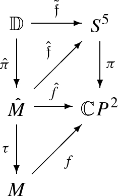
  where ${\hat{{\mathfrak {f}}}} : {\hat{M}} \rightarrow S^5$ is the naturally global lift of ${\hat{f}}$. Then, either ${\hat{M}} = M$ and f itself has a global lift or $\tau : {\hat{M}} \rightarrow M$ has order three and ${\hat{M}}$ has the global lift ${\hat{{\mathfrak {f}}}}$.

Proof

Since the image of c is either only the identity element of $S^1$ or the full group of cubic roots, the kernel of c either is all of $\pi _1 (M)$ or a subgroup $\Gamma$ satisfying ${\mathbb {A}}_3 \cong \pi _1(M) / \Gamma$.

In the first case ${\hat{M}} = M$ and ${\hat{{\mathfrak {f}}}}$ actually is a global lift of f. In the second case, the map ${\hat{f}} : {\hat{M}} \rightarrow \mathbb {C}P^2$ has a global lift, namely ${\hat{{\mathfrak {f}}}} : {\hat{M}} \rightarrow S^5$. $\square$

Corollary A.7

Let M be a Riemann surface different from $S^2$ and $f: M \rightarrow \mathbb {C}P^2$ an immersion without complex points. Then either f has a global lift ${\mathfrak {f}}: M \rightarrow S^5,$ or there exists a 3-fold covering $\tau : {\hat{M}} \rightarrow M$ of M such that the immersion ${\hat{f}} = f \circ \tau : {\hat{M}} \rightarrow \mathbb {C}P^2$ has a global lift, while the given $f : M \rightarrow \mathbb {C}P^2$ has not.

References

Black, M.: Harmonic Maps into Homogeneous Spaces. Pitman Research Notes in Mathematics Series, 255. Longman Scientific & Technical, Harlow, Wiley, New York (1991)
Burstall, F.E., Pedit, F.: Harmonic maps via Adler-Kostant-Symes theory, Harmonic maps and integrable systems. In: Fordy, A.P., Wood, J.C. (eds.) Aspects of Math, vol. 23, pp. 221–272. Vieweg, Braunschweig, Wiesbaden (1994)
Castro, I., Urbano, F.: New examples of minimal Lagrangian tori in the complex projective plane. Manuscripta Math. 85, 265–281 (1994)
Dorfmeister, F.J., Kobayashi, S.-P.: Timelike minimal Lagrangian surfaces in the indefinite complex hyperbolic two-space. Preprint, arXiv:1909.04818 (2019)
Dorfmeister, F.J., Ma, H.: Some new examples of minimal Lagrangian surfaces in \({\mathbb{C}}P^2\). (in preparation)
Dorfmeister, J.F., Wang, E.: Definite affine spheres via loop groups I: general theory (in preparation) (2019)
Dorfmeister, J., Eitner, U.: Weierstraß-type representation of affine spheres. Abh. Math. Sem. Univ. Hamburg 71, 225–250 (2001)
Dorfmeister, J., Pedit, F., Wu, H.: Weierstrass type representation of harmonic maps into symmetric spaces. Commun. Anal. Geom. 6(4), 633–668 (1998)
Dorfmeister, J.F., Freyn, W., Kobayashi, S.-P., Wang, E.: Survey on real forms of the complex \(A_2^{(2)}\)-Toda equation. Complex Manifolds 6, 194–227 (2019)
Forster, O.: Lectures on Riemann Surfaces. Graduate Texts in Mathematics 81. Springer, Berlin (1981)
Li, A., Wang, C.: Geometry of surfaces in \({\mathbb{C}}P^2\) (preprint)
Loftin, J., McIntosh, I.: Minimal Lagrangian surfaces in \(C H^2\) and representations of surface groups into \(SU(2,1)\). Geom. Dedicata 162, 67–93 (2013)
Ma, H., Ma, Y.: Totally real minimal tori in \(\mathbb{C}P^2\). Math. Z. 249(2), 241–267 (2005)
McIntosh, I.: Special Lagrangian cones in C3 and primitive harmonic maps. J. Lond. Math. Soc. 67(2), 769–789 (2003)
Mironov, A.E.: The Novikov–Veselov hierarchy of equations and integrable deformations of minimal Lagrangian tori in \(\mathbb{C}P^2\). (Russian) Sib. Elektron. Mat. Izv. 1, 38–46 (2004). arXiv:math/0607700v1)
Okuhara, S.: A construction of special Lagrangian 3-folds via the generalized Weierstrass representation (English summary). Hokkaido Math. J. 43(2), 175–199 (2014)
Ruh, E.A., Vilms, J.: The tension field of the Gauss map. Trans. Am. Math. Soc. 149, 569–573 (1970)
Wang, C.: The Classification of Homogeneous Surfaces in \(\mathbb{C}P^2\), Geometry and Topology of Submanifolds, X (Beijing/Berlin, 1999), pp. 303–314. World Science Publishing, River Edge (2000)
Author information
Authors and Affiliations
Corresponding author
Additional information
Publisher's Note
Springer Nature remains neutral with regard to jurisdictional claims in published maps and institutional affiliations.
Shimpei Kobayashi is partially supported by JSPS KAKENHI Grant number JP18K03265. Hui Ma is partially supported by NSFC no.11831005, no.11671223 and no. 11961131001.