Power system resilience quantification and enhancement strategy for real-time operation

Abstract

The increased occurrence of extreme weather events worldwide has changed the way power system reliability is determined. The effect of high intensity weather events has catastrophic effects on power system operation, and the determination of its effect is a very important and timely requirement. The conventional reliability evaluation methods used in power systems require knowledge of historical datasets, which may not be available in the case of an extreme event as these events have a low probability of occurrence. Hence, new methods to quantify power system resilience are needed. This paper uses a self-organizing map (SOM) to compute the resilience of any network using only system information, no historical data are required. The use of SOM makes the resilience quantification process very fast, and hence resilience can be evaluated in real-time during any catastrophic event, and correspondingly, action can be taken to improve the resilience of the system using available resources in the most suitable way so that the system can glide through the extreme event with the best possible performance. The paper first details the SOM-based resilience quantification method and then proposes a two-stage resilience improvement strategy using existing resources connected to the system based on the resilience value calculated in real-time during the progression of the event. The proposed quantification method and the resilience improvement strategy are tested on the IEEE 33 bus and 69 bus distribution systems. The results show that the resilience improved from 0.45 to 0.95 and 0.65 to 0.85 for the two systems, respectively, which proves the effectiveness of the proposed methodology.

1 Introduction

In recent years, the frequent occurrence of catastrophic events has caused serious consequences for the power system [1]. There were 64% more significant power outages in the USA [2] during 2011–2021 compared to the earlier decade, and approximately 83% of all power outages reported between 2000 and 2021 were caused by weather-related incidents. In comparison with 2000–2010, the average yearly number of weather-related power disruptions increased by almost 78% between 2011 and 2021. In 2019, Typhoon ‘Lekima’ caused 168 power disruptions in lines, affecting 7.59 million users in coastal regions of China. Similarly, in 2014, typhoon ’Seagull’ caused numerous breakdowns in high-voltage transmission lines in Hainan Province of China and resulted in a blackout for 1.24 million users. And in more recent times in India, cyclone ‘Biparjoy’ ripped out 4,038 electricity poles, leading to power failures in many feeders with an estimated loss of more than Rs. 1013 crore. Therefore, the increase in extreme weather events in recent times has resulted in several power disruptions and economic losses [3] worldwide. Consequently, the power system’s vulnerability to these extreme weather events has gained more attention.

These weather events have a high impact on the system; however, the probability of repeated occurrences of such events on the same network is very low, so the data availability corresponding to these events is very poor, hence they are categorized as high impact low-frequency (HILF) events. Electric grid operators have traditionally considered reliability to be a key indicator of the system’s performance, which requires a historical set of data of similar events. But, as recent years have witnessed a rise in the frequency and severity of HILF extreme weather occurrences without having historical data for the same, the grid operators are focusing on a different performance index, namely resilience, to analyze the power system’s performance for similar events. The resilience of the power system is determined by the system’s capability to absorb and recover from these HILF events in order to function satisfactorily [4]. Resilience is described as “The ability of a system to degrade gracefully under extreme perturbations, and recover quickly after the events have ceased” [5].

In recent times, occurrence of this type of events resulted in extended outages and major financial losses [6, 7]. Moreover, aged power system infrastructure substantially affects the frequency of occurrence and expenses of long outages [8, 9]. Increasing resilience and evaluating options to reduce the occurrence and effect of power outages are of interest for power system planners and operators [10, 11].

To evaluate the performance of power system during extreme weather conditions, we need to first quantify the power system resilience [12]. A significant amount of research has proposed methods for quantification and evaluation of the resilience of power system, which can be categorized into two groups—probabilistic and analytical. A probabilistic modeling method is used for resilience quantification with the help of a system performance and restoration model, event model and fragility model of the equipment. By simulating various scenarios using Monte Carlo simulations, the model can predict the probability of power outages and their potential impact on the grid infrastructure. An automated framework presented in [13] utilizes weather and power outage data to quantify power system resilience, aiding in vulnerability identification and development of planning and predictive analysis tools. An example of an analytical approach is the application of reliability theory to assess the resilience of a power transmission network. By modeling the network topology, component reliability and failure probabilities, analysts can identify critical components and assess the system’s vulnerability to disruptions. Analytical techniques such as fault tree analysis can help evaluate the cascading effects of failures and identify strategies to enhance system resilience, such as implementing redundancy or improving maintenance practices [14].

But the event model, i.e., the modeling of extreme weather conditions, is very difficult. Moreover, presently available power system reliability calculation methods largely depend on probability and require a large amount of historical data related to the event [15]. On the other hand, in analytical category methods, different scenarios of the event are considered for which simulations are performed, and the performance is measured analytically. This group of methods is again divided into two sub-groups—complex network-based and power flow-based approach. In the complex network sub-group, the graph of the network is analyzed, and the parameters that may affect the electrical infrastructure’s resilience are assessed.

In [16], Choquet integral (CI) method is used for the quantification of power system resilience using parameters decided using graph theory having a multi-criteria decision-making approach. The second approach is power flow-based. In this type of method, different attack scenarios are considered to evaluate system hardening and restoration measure. A duration dependent value of resilience is calculated, and it is incorporated into the investment related decision-making process for resilience improvement in [17]. A two-step stochastic mixed integer programming method proposed in [18] determines system hardening cost in the first stage, and costs incurred during HILF events in a distribution system are determined at the second level. A two-stage analysis is presented in [19] to explain the impact of microgrids in increasing the resilience of the electrical network. The authors perform a cost–benefit analysis [20] of preventive maintenance, considering the cost of preventive maintenance and that of resilience. For the implementation of various scenarios, resilience indicators, reliability and cost analysis have been analyzed. The simulation results for a number of scenarios are observed, and based on the analysis, the preventive maintenance schedule is chosen that will be able to improve the reliability and resilience of the system to the best value in case of an extreme event.

In [21] a two-stage resilient restoration model is proposed utilizing Electric Vehicles (EVs) and Mobile Energy Resources (MERs) to mitigate outage impacts. The resilience improvement method proposed in [22] is based on two key components: installing intelligently controlled remote switches and optimizing distributed generation capacity while considering the critical loads present. It aims to ascertain suitable zones by taking into account the constraints and limits of the distributed generation. While [23] proposes an optimization-based strategy to detect the optimal location for setting up new tie line in the power distribution system. It assesses the importance of tie line construction to improve the performance of the distribution system by restoration following any HILF events.

The accurate quantification of resilience is difficult as many factors affect it. The methods used in previous works combine the factors of resilience metrics in a suitable form such as the mathematical integration method, factor measurement and selection and assignment of suitable weight, which are debatable. Quantifying resilience accurately needs a commonly acceptable algorithm and a related measure. Further, existing methods, such as the weighting method, needs a weight to be assigned on the system parameters being considered such as the criticality of powerlines, diversity and capacity distribution of distributed energy resources (DERs), which may vary according to the system. Therefore, assessing the system parameters, which should be dominating toward increasing and decreasing resilience becomes a difficult task, which further makes assigning weights to the resilience parameters harder. Thus, weight assignment methods depend on the system operator’s interpretation and are typically subjective. The method in [24] uses SOM to quantify resilience and, in turn removes any subjective weight assignment requirement as the neuron learns during training which system parameters are dominating toward increasing and decreasing resilience, and they arrange themselves based on the relative importance of those system parameters. But the proposed work does not include a wide variety of system factors in resilience calculation, like hardening of power lines, aging of assets, etc., that have a potential impact on critical load survivability in an HILF event. To fill this research gap, the present paper proposes a quantification method that includes a wide variety of system factors that affect the resilience of the power system.

The proposed SOM-based method uses only the operating conditions of any power system network and the availability of different generation, load conditions; it does not require the modeling of the extreme weather conditions due to which resilience is being determined. The SOM-based resilience quantification is used as evaluation tool, namely RSOM, capable of calculating the resilience of a given network in real-time without the requirement of historical data of extreme events.

Once resilience quantification is complete, the next step is to improve the resilience in case of low resilience. Numerous researchers have proposed resilience enhancement strategies for improving resilience in power system operation. To improve the operational resilience of power grids [25, 26], present a probabilistic proactive generation redispatch strategy and proposes an optimization-based recovery method that takes sequence of system reconfiguration and repair into account. Adjusting system configuration is a technique to meet consumer demand while minimizing losses [27] without neglecting load variations in reconfiguration model [28].

For both preventative and emergency situations [29], proposes an integrated resilience response model. Additionally [30], proposes an optimization approach that takes infrastructure network restoration scheduling into account. But resilience enhancement is mostly done once the extreme event has occurred, i.e., the actions are taken after disturbance to improve the system’s ability to withstand similar events in the future [31]. Proposes a novel multistage restoration technique by critical load restoration to enhance the network’s resiliency after the fault occurrence and blackout. The actions that are taken into consideration are switching operations and weighted restored energy, which provides the optimal restoration plan for every hour of outage. Post-event resilience enhancement may not fully mitigate the impact of future disturbances, while the measures can improve the system’s ability to cope with specific scenarios, they might not address all potential vulnerabilities.

In view of the above, the present paper proposes the following contributions:

• A fast and efficient resilience quantification methodology to evaluate a system’s resilience based on its network states, without the requirement of historical data of the extreme event, enabling determination of resilience of any network in real-time.

• The proposed quantification method takes into account a wide variety of system factors like connectivity of the lines, availability of local generation, hardening of power lines and aging of assets, etc., which has potential impact on critical load survivability in the case of an HILF event.

• A resilience enhancement strategy for real-time operation is proposed for the power distribution system. For enhancing the critical load survivability in extreme weather conditions, a resilience operation method is developed, detailing step by step operation in real-time and with some delay.

• Unlike previous studies that have primarily used resource-constrained methods to improve resilience, the present paper proposes a framework for resilient operation of the power distribution system that can be used in real-time to improve the resilience in the case of HILF events.

The proposed resilience quantification is based on SOM, and once the RSOM network is trained, it can provide the resilience value of any network in real-time. The details of a basic SOM network and its training are detailed in the next section. It also describes how the RSOM works to determine the resilience of the given power system, i.e., the input parameters, clustering technique and operating principle of the RSOM.

This paper is organized as follows: Sect. 2 presents the basics of SOM and the mathematical formulation of input parameters, the resilience quantification model (RSOM) and its performance evaluation, the steps involved in resilience quantification, training of RSOM and implementation of RSOM for real-time operation. Section 3 presents the proposed resilience enhancement strategy in real-time for the distribution system. Section 4 presents results, discussion and future scope by analyzing different cases, and finally, Sect. 5 presents a conclusion.

2 Resilience quantification method based on self-organizing map

2.1 Basics of SOM

SOM is an unsupervised, competitive learning-based neural network (NN) that is widely utilized to cluster data without knowing in advance which classes the input data belong to or how important each class is to the cluster [32]. Because of this characteristic, SOM is used in this paper as an aggregation technique to compress a set of features to a scalar value, and there is no need of weight assignment for the inputs. Figure 1 shows the flowchart of the process illustrating how the SOM learning-based clustering technique works.

Fig. 1

Basic steps of SOM training method

2.2 Parameters affecting resilience of power system

The resilience of a power system network depends on multiple factors related to the system’s operating and physical condition. The parameters that affect system resilience are mentioned in previous works [33, 34]. These parameters are divided into static and dynamic groups on the basis of their time-invariance nature. The most important parameters which closely affect the system reliance and based on which the power system resilience value can be calculated, are listed below on the basis of their relative importance to improve the resilience of the system.

The parameter “Cyber security of automation infrastructure” included in previous work [24] is not taken into consideration in this work as the present work is based on HILF events related to weather conditions only and “average asset level resilience” is modified to “reliability of asset” considering the aging of different equipment and their failure probability.

Hardening of power lines

Hardening means strengthening the power system infrastructure against extreme events. Undergrounding the wires is an effective procedure for increasing system resilience. This parameter is used as one input training feature of the RSOM and is defined by Eq. (1):

$${{R}^{H}}_{=}\frac{N(H)}{{N}^{T}}$$

(1)

${R}^{H}= \text{Hardening\, resilient \,factor \,of \,power \,lines}.$

The hardening resilient factor of the power system is 1 if all the lines are undergrounded and it is 0 when none of the lines are undergrounded.

Reliability of assets

The reliability of an asset is the ability of the asset to perform under certain conditions over a specified period without breaking down. The lifetime of the power system equipment is defined in the following three different ways:

Physical lifetime

The time duration for a piece of equipment from the start of operation to the status when the equipment is not usable in the normal operating condition and needs to be replaced. The physical lifetime of the equipment can be prolonged by preventative maintenance.

Technical lifetime

The equipment may be physically usable but need to be replaced due to technical reasons. For example, a new technology is developed for equipment and spare parts are no longer produced.

Economic lifetime

The equipment may be physically usable but no longer valuable economically.

The reliability of assets is a very important aspect for power system resilience calculation and hence needs to be incorporated into the RSOM training data. The reliability of an asset is related to the failure probability of an asset. The failure probability of the asset mostly depends upon four factors; aging, loading, maintenance and external conditions. The decisions that distribution system managers must take include when to replace an asset, when to repair or overhaul an asset, when to maintain an asset and when to do nothing. Table 1 represents the perceived risks [35] of different types of equipment considering aging as the main factor and the time needed to repair these equipment in case of failure.

Table 1 Risks of equipment

Therefore, reliability of asset resilient factor is defined as:

$${R}^{A}=1-F\left(p\right)$$

(2a)

The failure probability of the assets, F(p), is defined by Eq. (2b):

$$ F\left( p \right) = \frac{{\mathop \sum \nolimits_{i = 1}^{n} f_{i} *N_{i} }}{{\mathop \sum \nolimits_{i = 1}^{n} N_{i} }} $$

(2b)

${f}_{i}$ = Failure probability of asset component. ${N}_{i}$ = Total number of component.

Geographic and capacity distribution of DERs

If the DERs connected in a distribution system have enough generating capacity and these DERs are geographically distributed throughout the system, then even in the case of extreme weather events that damage parts of the distribution system, most of the critical loads will continue to receive power during the extreme event. On the other hand, if the DERs are not distributed throughout the system, an extreme weather event may isolate a part of the distribution system and then it will not be able to support the critical loads present in the isolated part. The resilient factor used as input to RSOM that represents the diversity of DG is defined by Eq. (3a).

$${R}^{\rm{GD}}= \frac{{\text{Diversity}}^{\rm{G}}}{{\text{Diversity}}^{\rm {L}}}$$

(3a)

$$\text{Diversity}^{G}=\frac{{\sum }_{i=1}^{{N}_{G}}\sum_{j=1,}^{{N}_{G}}{Gen}_{i}^{m}{Gen}_{j}^{m}{D}_{ij}^{G}}{{D}_{\text{max}}^{G}{\sum }_{i=1}^{{N}_{G}}\sum_{j=1,}^{{N}_{G}}{Gen}_{i}^{m}{Gen}_{j}^{m}}$$

(3b)

i and j are the indices of generator, where i ≠ j

$${\text{Diversity}}^{\rm L}=\frac{{\sum }_{i=1}^{{N}_{L}}\sum_{j=1,}^{{N}_{L}}{ldc}_{i}^{m}{ldc}_{j}^{m}{D}_{ij}^{G}}{{D}_{\text{max}}^{L}{\sum }_{i=1}^{{N}_{L}}\sum_{j=1,}^{{N}_{L}}{ldc}_{i}^{m}{ldc}_{j}^{m}}$$

(3c)

i and j are the indices of critical load, where i ≠ j

$${D}_{ij}^{G}=\sqrt{{\left({x}_{i}^{G}-{x}_{j}^{G}\right)}^{2}+{({y}_{i}^{G}-{y}_{j}^{G})}^{2}}$$

(3d)

$${D}_{ij}^{L}=\sqrt{{\left({x}_{i}^{L}-{x}_{j}^{L}\right)}^{2}+{({y}_{i}^{L}-{y}_{j}^{L})}^{2}}$$

(3e)

where

$x_{i}^{G}$, $y_{i}^{G} , x_{i}^{L}$, $y_{j}^{L}$ ith generator and jth load coordinates, respectively.

${D}_{\text{max}}^{G}$, ${D}_{\text{max}}^{L}$ Maximum distance among all generator nodes and load nodes, respectively.

Power line non-criticality To determine the effect of critical line failure it must be defined how critical a line connecting the generator and load nodes are. The parameter ${R}^{C}$ is defined as the criticality of paths by Eq. (4)

$${R}^{\rm{NC}}=\sum_{i=1}^{N}\sum_{j=1,i\ne j}^{N}\frac{\sum_{i=1}^{P(i,j)}E({L}_{q}\left(i,j\right)*{W}_{q}\left(i,j\right)-1)}{E(p(i,j))}$$

(4)

where p(i, j) is the path connecting generator i and load j; ${L}_{q}\left(i,j\right)$ is a line q in this path; E(.) represents electrical distance;${W}_{q}\left(i,j\right)$ number of times a line ${L}_{q}\left(i,j\right)$ appears for all paths between ith generator and jth load. In the RHS of the above equation the second term tells us the amount of overlap of the lines existing in paths between ith generator and jth load. If any line ${L}_{q}\left(i,j\right)$ appears once only in all possible paths, ${W}_{q}\left(i,j\right)$ = 1, and hence the line will be considered to be non-critical. But, if the line ${L}_{q}\left(i,j\right)$ appears multiple times in the paths, the line will be critical and hence ${W}_{q}\left(i,j\right)$ will be considered greater than 1, and will lead to reduction in the value of ${R}^{\text{NC}}$.

Critical load sustainability

A critical load is defined as the load that is always required to maintain an uninterrupted power supply. DERs such as DG, PV and BESS ensure continuity of power supply. Hence, the input parameter to the RSOM to incorporate this characteristic is given by Eq. (5) as follows:

$${R}^{L}=\sum_{t=1}^{T}\left(\frac{\sum_{i=1}^{N}\left[{G}_{n}\left(t\right)-{L}_{n}^{c}(t)\right]}{T\sum_{i=1}^{N}{G}_{n}\left(t\right)}\right)$$

(5)

where t represents the time slot index for the range T = {ζ, ζ + 1, ζ + 2, …}, ${L}_{n}^{c}(t)$ is amount of the critical load connected to node n, and ${G}_{n}(t)$ is amount of local generation at node n.

Energy reserves availability The distribution system will be able to ride through an extreme event if there is sufficient reserve present in the form of local generators like diesel-based DG, BESS, etc. Thus, the existence of such reserves and their effective use have a significant impact on resilience, and this factor is defined by Eq. (6)

$$\begin{aligned}{R}^{\rm{ER}}&=\sum_{t=1}^{T}\left(\frac{\sum_{x=1}^{N}[{D}_{x}\left(t\right)-{F}_{x}{G}_{x}(t)]}{T\sum_{x=1}^{N}{F}_{x}{G}_{x}(t)}\right. \\ &\quad +\left. \frac{\sum_{x=1}^{N}[{B}_{x}\left(t\right)-{\eta }_{x}{p}_{bx}(t)]}{T\sum_{x=1}^{N}{\eta }_{x}{p}_{bx}(t)}\right) \end{aligned}$$

(6)

where ${D}_{x}\left(t\right)$ is availability of diesel for xth DG at time t, ${F}_{x}$ is the function that relates the power output of diesel DG and its diesel consumption;${B}_{x}\left(t\right)$ is SOC of xth BESS at time t and the efficiency of this BESS is ${\eta }_{x}$, and ${p}_{bx}(t)$ is its active power. Therefore, RHS of the equation calculates the availability of diesel and the remaining SOC level of the BESS to be dispatched.

Since generators have a set revolution per minute (RPM), the fuel consumption of these generators at different load levels can be estimated. Table 2 provides an estimate of a diesel generator’s fuel consumption [36] based on the generator’s size and the load it is supplying.

Table 2 Diesel generator approximate fuel consumption in liters

Network reconfiguration capability A distribution system connected to tie-switches can improve its resilience to incidents through network reconfiguration, involving the potential for multiple islanding scenarios, and integrating loads as well as DERs distributed across various geographic regions. The possible count of islands produced depends on the quantity and placement of switching devices. The practicality of these islands can be defined based on adequate generation availability on the individual islands, voltage limits, etc. As a result, ${R}^{\rm{NRC}}$ measures the number of feasible islands as shown in Eq. (7).

$${R}^{\rm{NRC}} =\frac{\sum_{t=1}^{T}argmax{N}_{ISLD}\sum_{y=1}^{{N}_{ISLD}}\left([\sum_{x=1}^{{N}_{y}}\left({G}_{xy}-{L}_{xy}^{c}\right)]+\sum_{x=1}^{{N}_{y}}\left[{V}_{\text{max}}-{V}_{xy}\left(t\right)\right]+ \sum_{x=1}^{{N}_{y}}\left[{V}_{min}-{V}_{xy}\left(t\right)\right]\right)}{Tn(N)}$$

(7)

where ${N}_{ISLD}$ represents the possible islands; ${N}_{y}$ is the set of nodes available in island y, ${G}_{xy}$, is the generation at xth node present in yth island. ${L}_{xy}^{c}$ is the amount of critical load connected and ${V}_{xy}\left(t\right)$ is voltage at xth node of y-this land, respectively.

Availability of redundant path

The probability of maintaining power supply to loads during various extreme conditions increases with the increase in connecting paths between these loads and the available DERs; hence, the normalized value of possible paths connecting any generator(s) with the critical load should be used as a parameter for calculating resilience. This parameter is called the path redundancy resilient factor (${R}^{\rm{PATH}}$), which is represented by Eq. (8).

$$ R^{\rm{PATH}} = \frac{{\mathop \sum \nolimits_{j = 1}^{N} \mathop \sum \nolimits_{i = 1}^{N} \frac{1}{{\mathop \sum \nolimits_{q = 1}^{Q} E(P_{q} \left( {i,j} \right)}}}}{{\frac{{n\left( N \right)^{2} }}{{2\overline{E}\left( {q\left( {i,j} \right)} \right)}}}} $$

(8)

where P_k(i, j) is the qth path from node i to j; $E({P}_{q}(i,j)$ and $\overline{E}$ (P_k(i, j)) are the electrical distance of the path and the maximum electrical distance, respectively.

Table 3 lists all the input parameters considered in training RSOM to determine resilience of any distribution system. These parameters are strongly related to resilience of the system in presence of an extreme weather event. From the table it is clear that the resilience metric considered in RSOM consists of eight input parameters which are given as—${R}^{H},{R}^{A}, {R}^{\rm{GD}},{R}^{\rm{NC}},{R}^{L},{{R}^{\rm{ER}},R}^{\rm{NRC}}{,R}^{\rm{PATH}}$

Table 3 Parameters affecting resilience of the distribution system with their characterization in RSOM

2.3 Structure of resilience quantifier RSOM and its performance evaluations

In order to evaluate the time-varying resilience of the system, it is expected that real-time data are available to the Distribution System Operator (DSO) from the SCADA system, i.e., the connectivity of the system, the real power generation capacity and demand, the amount of energy reserve and its location, etc. Table 3 lists the input parameters required by DSO and the relevant feature outputs that are taken as RSOM inputs.

SOM proves to be a suitable method as an aggregation technique to combine and compress multiple features of the power system under evaluation to a scalar value resilience (${\mathbb{R}}$) without the need of any weight assignment to inputs. Figure 2 shows the SOM model for resilience evaluation. This method allows real-time decision-making by using only the power system’s existing condition, like demand, generation and system connectivity. A one-dimensional SOM model RSOM is used to derive a scalar value resilience index, for a given collection of features or resilience parameters. One-dimensional SOM offers simplicity in structure, comprising a linear array of neurons, facilitating easy visualization and interpretation. Their ability to capture linear or sequential patterns makes them well-suited for tasks involving one-dimensional or sequential data structures. Additionally, one-dimensional SOM are computationally efficient, requiring fewer resources, thus making them viable for large-scale or real-time applications. Hence, the employment of a one-dimensional SOM in the RSOM approach ensures efficient aggregation and interpretation of feature vectors, addressing the objectives of resilience quantification effectively.

Fig. 2

The resilience quantification model RSOM

While two-dimensional SOMs offer the advantage of capturing more complex relationships and structures in the data, they also introduce additional complexity in interpretation and computation. Therefore, the choice between one-dimensional and two-dimensional SOMs depends on the specific requirements of the resilience quantification task and the characteristics of the dataset.

Initially, the RSOM is trained using features across various system states, with each state (alongside its associated feature set) mapping to a distinct neuron. This linear array of neurons serve as a scale denoting resilience, ${\mathbb{R}}$, ranging between 0 and 1, and may be represented mathematically as below:

${\mathbb{R}}$ = SOM (${R}^{H},{R}^{A},{R}^{\rm{GD}},{R}^{\rm{NC}},{R}^{L},{R}^{\rm{ER}}{R}^{\rm{NRC}},{R}^{\rm{PATH}}$).

Through RSOM, each resilience parameter is represented by a node on the SOM grid, and the proximity of these nodes reflects the similarities between the parameters. The resilience index is then determined based on the position of the input parameters relative to the SOM grid. This index provides a concise measure of the overall resilience, condensing the multidimensional information of the resilience parameters into a single numerical value.

By employing RSOM, complex sets of resilience parameters can be effectively condensed and quantified, enabling a comprehensive assessment of resilience of various systems at different operating conditions.

As discussed above, a SOM-based method is proposed [24], which removes some of the disadvantages of the subjective weight assignment method, but there are few limitations to this proposed method. Though multiple input parameters are considered during resilience calculation, some important factors were missed out, like the connectivity of the lines, the availability of local generation, hardening of power lines and the aging of assets etc. that could potentially impact critical load survivability in an HILF event.

The effectiveness of SOM heavily relies on the characteristics and dynamics of the specific system under study, limiting their applicability to broader domains or diverse datasets. In its basic form, the SOM is not apt for resilience quantification due to the potential lack of smoothness and uniform gradient in the mapping of inputs to neurons across the network. To handle this, in the present paper, the SOM’s training data are added with two sets of artificially generated datasets: one characterizing characteristics for maximum resilience and the other representing the minimal resilience. For instance, the most resilient system may boast ample DERs at each load node and a robust decentralized control system. Conversely, the least resilient system might lack DERs, relying entirely on a vulnerable bulk power source, an unreliable bulk grid. So, the training data consists of a large set generated from system operating condition along with a considerable set of data representing maximum and minimum resilience conditions.

For RSOM, training is done using ${N}^{P}$ neurons. The neighborhood function’s initial value starts at ${N}^{P}$ and steadily decreases over the course of iterations, according to a Gaussian distribution. Thus, each neuron’s starting impact zone is the complete array of ${N}^{P}$ neurons. The learning rate indirectly influences the extent of this adjustment. A higher learning rate implies more significant adjustments to neuron weights, potentially leading to faster convergence but also increasing the risk of overshooting optimal solutions. Conversely, a lower learning rate results in more conservative adjustments, which may lead to slower convergence but with potentially more stable and precise results. This is represented by Eq. (9)

$${W}_{ij}\left(t+1\right)={W}_{ij}\left(t\right)+\alpha\left(t\right)*{h}_{ij}(t)({X}_{j}-{W}_{ji}\left(t\right))$$

(9)

where ${W}_{ji}(t)$ is the weight between neuron i and its input j at time t. α(t) is the learning rate at time t. ${h}_{ij}$(t) is the neighborhood function at time t, determining the influence of the neighboring neurons. ${X}_{j}$ is the input to the SOM.

Repeated training of the RSOM will teach the neurons’ smaller effect zones to recognize a smooth gradient mapping of the input data. Once the RSOM is trained, it can be used to determine the resilience of any distribution system even the one which is not used earlier during training of RSOM. The mapping of inputs to the output neuron is adjusted in the proposed RSOM approach as follows.

• The neurons located at ends are compelled to learn two hypothetical conditions: the best hypothetical condition that would make it the most resilient, and the worst hypothetical condition having minimum resilience value.

• A neuron has only two neighbors within a radius of 1 (or a single neighbor if the neuron is at the end of the line). During the training process, the network first identifies the winning neuron for each input vector. Each weight vector then moves to the average position of all of the input vectors for which it is a winner or for which it is in the neighborhood of a winner. The distance that defines the size of the neighborhood is altered during training in two phases.

• The first is the ordering phase, In which the neighborhood distance starts at an initial distance and decreases to the tuning neighborhood distance (1.0). As the neighborhood distance decreases over this phase, the neurons of the network typically order themselves in the input space with the same topology in which they are ordered physically. The second phase is the tuning phase, which lasts for the rest of training or adaptation; the neighborhood size decreases below 1, so only the winning neuron learns for each sample.

• For the set of input parameters related to a new distribution system for which resilience is calculated, a neuron will be selected. Let’s assume, neuron n got selected corresponding to the tested operating system condition, then the system resilience will be in the range (${N}^{P}-\frac{n}{{N}^{P}}, {N}^{P}-(n+1)/{N}^{P})$, and we then calculate the system resilience metric as follows:

  $${\mathbb{R}}=1-\left(\frac{n-0.5}{{N}^{P}}\right)$$

  (10)

The neuron 1 corresponds to the minimum value of resilience, which is 0, and the last neuron N^P corresponds to the highest possible value of resilience, i.e., 1.

Performance evaluation of SOM

The trained RSOM need to be evaluated to check how effective its performance is. The following parameters are used to determine the performance [37] of the RSOM.

Quantization error

It is the average error measured by Euclidean distance, i.e., the mean Euclidean distance between a data sample and its best-matching unit, which is represented by Eq. (11):

$$\text{QE}\left(\left\{{m}_{k}\right\},\mathcal{X}\right)=\frac{1}{N}\sum_{i=1}^{N}{\Vert {x}_{i}-{m}_{{b}_{i}}\Vert }_{2}$$

(11)

where

${x}_{i}$ is the Input data, ${b}_{i}$ is the best-matching unit of ${X}_{i}$, ${b}_{i}$ is ${\text{argmin}}\Vert {X}_{i}-{m}_{{b}_{i}}\Vert$,${m}_{k}$ is the weight and The set of input data samples is denoted as $\mathcal{X}=\left\{{x}_{i}\right\}1\le i\le N,$

Unsupervised clustering accuracy

It is defined as the number of samples assigned to the correct class divided by the total number of samples. It consists in the accuracy of the resulting classification using the best one-to-one mapping m between clusters and class labels, which is represented by Eq. (12):

$$ {\text{Acc}}\left( {Q,Y} \right) = \frac{1}{N}{\text{max}}\mathop \sum \limits_{k = 1}^{K} \left| {Q_{k} \cap Y_{m\left( k \right)} } \right| $$

(12)

$Q = \left\{ {Q_{k} } \right\}{,}\;k = \, 1 \ldots K$, K is the sets of data points belonging to each cluster, for external indices, we assume labels are associated to each sample, with to C different classes. We note Y = {Y_j}, j = 1…C the sets of elements belonging to each class.

2.4 Resilience quantification using RSOM

RSOM-based resilience quantification consists of two separate parts: offline training and real-time evaluation. Figure 3 represents the proposed step-wise approach for the quantification of resilience using RSOM for both offline and real-time evaluations. The RSOM is trained (offline training before putting the tool at work) using a large number of system operating conditions, and the output neuron is assigned a numerical value between 0 and 1, for every group as per the system’s resilience condition. Once trained, the RSOM is capable of classifying any operating condition of the system and generate the resilience value in real-time. The process is detailed below:

Fig. 3

Flowchart of RSOM-based resilience quantification method

Offline training

Once the system under consideration is known, the information regarding operating states of the system and its components are collected from SCADA/smart meters connected with the distribution system.

The information gathered from the distribution system is pre-processed, i.e., used to determine the input parameters of the RSOM using Eq. (1–8).The training dataset is generated and RSOM is trained using this data.

Real-time evaluation Collect the system operating scenarios from the SCADA system or smart meters connected and determine the corresponding input parameters for RSOM using Eqs. (1–8). For this set of input, the already trained RSOM will classify the system’s operating state resilience in real-time.

The effectiveness and superiority of the proposed resilience quantification is demonstrated on The Enhanced IEEE 33 Bus [38] and, The Modified IEEE 69 Bus Test Distribution Systems [39] presented in Figs. 4 and 5, respectively. Some of the lines are considered to be hardened and, here, fourteen and twenty-nine lines are hardened in the Enhanced IEEE 33 and Modified 69 Bus Test Distribution System, respectively, which are shown by the red color in the figures; these lines are chosen randomly and include critical lines. Further, for the calculation of input parameters for RSOM, it is assumed that bus 1 is located at the origin (0, 0) and the distance between any two consecutive bus is 5 km [40].

Fig. 4

The enhanced IEEE 33 bus distribution test system

Fig. 5

The modified IEEE 69 bus test distribution system

The input parameters for the RSOM are calculated for the IEEE 33 bus and IEEE 69 bus systems to generate the training scenarios, only 10 such random training samples for IEEE 33 bus system are shown here, in Table 4. The value of resilience, calculated by the RSOM, once the RSOM training is completed, is also shown in this table.

Table 4 Resilience for 33 bus system for different operating conditions

3 Real-time operation for distribution system resilience improvement

The capacity of a power system to endure and recover from disturbances, outages or external threats while sustaining the delivery of essential electrical services to consumers is referred to as resilience enhancement. Building a resilient power system is essential for ensuring the stability, dependability and safety of the power supply, particularly during adverse occurrences such as natural disasters, cyber-attacks, equipment failures and other emergencies. A two-step resilience enhancement strategy has been proposed in this paper which is shown in Fig. 6 having steps mentioned below:

• In order to evaluate and improve the system’s time-varying resilience, the data are fed from the SCADA system to RSOM, a tool being created for resilience quantification whose values lie between 0 and 1.

• The RSOM determines the ${\mathbb{R}}$ value for the present operating scenario.

• A predefined threshold value of resilience is set, if the measured resilience value is greater than the threshold resilience (i.e., ${\mathbb{R}}>{\mathbb{R}}_{\rm{TH}}$), it means the system is maintaining the required resilience and no action is required.

• Else, when ${\mathbb{R}}<{\mathbb{R}}_{\rm{TH}}$, some real-time action will be taken according to nature of catastrophic events, these actions may include tie line switching, load transfer, load shedding and the addition of temporary power generation (diesel generator).

• After considering this control action, power flow is performed on the modified system to check whether after the said action the system will continue to operate safely with operating conditions well within allowed limits, so as to avoid system overloading or instability.

• If yes, the control action is performed, otherwise other available actions are checked for the same condition and the action that allows system to operate within limit, is selected.

• Once the control action is performed, ${\mathbb{R}}$ is determined again using RSOM for the new operating condition, and if resilience still remains below the threshold value, a second-level control action, namely “Action with some delay” will be taken, which includes resource mobilization, mobile diesel generators and repair and replacement of equipment.

• Power flow is performed again on the modified system before applying the second-level control action so as to check the stability of the new operating condition. If the safety limits are maintained in power flow results, then only the action will be taken on the real operating system.

• This will continue until the required threshold value of resilience is achieved or all the possible actions are taken.

Fig. 6

Flowchart of proposed resilience enhancement strategy

3.1 Real-time action for resilience enhancement

Real-time actions are essential for improving resilience in a power system because they allow for quick and adaptable reactions to changing circumstances, disruptions or crises. These are some real-time actions that can be taken to enhance the resilience of the power system.

Tie line switching

Tie line switching is a technique used in power systems to improve resilience by optimizing power flow and boosting the system’s capacity to deal with contingencies or disruptions. During abnormal or emergency situations, the primary purpose of tie line switching is to shift power flows and prevent overloads on critical transmission lines. Tie line switching can assist avert major blackouts and keep the power system stable.

The equations governing tie line switching can be derived from the power flow and balance equations. Let’s denote.

${P}^{ij}$ = Power flow from area i to area j.

${P}^{ji}$ = Power flow from area j to area i.

$\Delta {P}^{i}$ = change in generation in area i.

$\Delta {P}^{j}$ = change in generation in area j.

$\Delta {P}^{ij}$ = change in power flow from area i to area j.

$\Delta {P}^{ji}$ = change in power flow from area j to area i.

The power balance equation for each area is:

$$\Delta {P}^{i}={ P}^{ij}-{P}^{ji}$$

(13a)

$$\Delta {P}^{j}={ P}^{ji}-{P}^{ij}$$

(13b)

When a tie line is switched, the change in power flow on that line is equal to the difference in the changes in generation for the two areas it connects:

$$\Delta {P}^{ij}= \Delta {P}^{i}- \Delta {P}^{j}$$

Similarly, $\Delta {P}^{ji}= \Delta {P}^{j}- \Delta {P}^{i}$

These equations help in analyzing and controlling power flow during tie line switching events in a power system. They are essential for ensuring the stability and reliability of the interconnected grid. The working of the tie line switch and how it contributes to resilience enhancement is described below.

Tie line switching allows multiple interconnections to exchange power between regions, and facilitates resource-sharing, allows load balancing between areas, establishes new islands, relieves overloads, aids in restoration after a catastrophic event. However, tie line switching needs to be done carefully because making the wrong choice might make things worse. So, tie line switching can help power networks become more resilient and so it is a component of a larger set of strategies meant to increase the resilience of power systems to unfavorable circumstances.

Load transfer and load shedding

Two important strategies used in power systems to increase resilience and system stability in unusual or emergency conditions are load transfer and load shedding. Both strategies aim to maintain system functionality and give priority to vital loads while striking a balance between supply and demand for electricity. The process of shifting power from one part of the electrical system to another in order to relieve overloads or approaching failures is known as load transfer. Tie line switching, as previously mentioned, may be used to do this by rerouting power flow between different areas or control locations. By distributing the load, load transfer avoids cascading failures and overloading generators or transmission lines. For example, if a generator or transmission line damages during an extreme event, the load can be moved to other healthy units or areas to ensure supply reliability. Load transfer may also be used to optimize power flows during normal operations, ensuring that generating resources are utilized efficiently and transmission congestion is kept to a minimum. Load shedding is the premeditated and systematic reduction of demand on the power system by shedding non-critical loads. Load shedding assists in matching available power supply with decreased demand during emergencies or extreme supply–demand mismatches, which subsequently helps in avoiding catastrophic system failure. Load shedding is frequently prioritized in order to safeguard critical loads such as hospitals, emergency services and important buildings, while nonessential or less crucial loads are shed in a regulated way. To ensure grid stability, advanced control technologies and real-time data analysis assist in detecting and shedding non-critical loads.

While load shedding is an efficient way to avert widespread blackouts and safeguard essential infrastructure, it should be used with caution to minimize customer interruptions and avoid social and economic consequences. Resilience enhancement through load transfer and load shedding is done to prioritize the critical loads connected to the system. Overall, load transfer and load shedding are critical techniques for improving power system resilience, allowing them to adapt to changing conditions, maintain stability and recover more quickly from disturbances. To guarantee prompt and suitable reactions to emergencies, these tactics are frequently linked with modern control and monitoring systems.

Temporary power supply solution

By providing backup power during emergencies, temporary power solutions can aid in enhancing the resilience of the power system. These fixes are meant to fill the void and maintain the operation of essential services until the primary power system is fully restored. Some popular temporary power options for increasing resilience are diesel generators and battery energy storage systems (BESS). BESS has a near-instantaneous response time. When the grid experiences fluctuations or sudden disruptions, BESS can rapidly discharge power to stabilize the system’s frequency and voltage, reducing the risk of cascading failures. The dynamics of SOC of the BESS can be described by Eq. (14a):

$$\frac{\text{dSOC}}{\text{d}t}=\frac{{P}_{i}-{P}_{o}}{{E}_{n}}$$

(14a)

where SOC is the state of charge, ${P}_{i}$ is power input (charging), ${P}_{o}$ is power output (discharging), ${E}_{n}$ is the nominal energy capacity of the battery. The charging and discharging power is calculated using battery voltage (${V}_{\rm bat}$).

Charging power:

$${P}_{i}=\frac{{V}_{bat}*{I}_{i}}{{\upeta }_{\rm{charge}}}$$

(14b)

Discharging power:

$${P}_{o}={V}_{\rm{bat}}*{I}_{O}*{\upeta }_{\rm{discharge}}$$

(14c)

where ${I}_{i}$ is the charging current, ${I}_{O}$ is the discharging current, ${\upeta }_{\rm charge}$ and ${\upeta }_{\rm discharge}$ are charging and discharging efficiencies. However, there are some considerations when implementing BESS for resilience enhancement; the capacity and duration of the BESS must be appropriately sized to meet the specific resilience requirements of the power system and the critical loads it aims to support. The maintenance and life cycle costs of BESS must be factored into the overall cost–benefit analysis.

Having a well-thought-out emergency response plan in place is essential when offering temporary power options. To guarantee temporary power supply solutions during emergencies and training for the responsible personnel for managing them are also crucial. In order to provide seamless backup power and facilitate quick recovery, temporary power solutions need to be correctly integrated into the power system’s overall resilience strategy.

3.2 Action with some delay

During an extreme incident resource mobilization for resilience improvement becomes even more vital. The goal is to minimize the impacts, encourage a prompt recovery and respond to the incident with efficiency and speed. The following are some of the key components of resource mobilization in these kinds of situations which will be enabled after the real-time actions fail to improve the systems resilience to the target value. The actions under this category are not real-time actions and require finite time to implement.

Emergency response teams

An emergency response team is a specialized group of individuals who are prepared to act swiftly and effectively in the event of a crisis or interruption. To enable smooth collaboration during crises, an efficient emergency response team for resilience enhancement needs thorough planning, preparation and coordination exercises. Reducing the effect of disruptions and quickly resuming power system operations are greatly aided by the team’s experience, preparedness and capacity for fast decision-making.

Mobile diesel generator

One essential tool for enhancing the resilience of the power grid is a transportable diesel generator. In the case of an emergency, it offers a versatile and portable supply of electrical power that can be quickly provided to critical locations. A mobile diesel generator can enhance the resilience of a power system by providing emergency backup power, temporary power restoration and mobility to support remote areas.

Repair and replacement of equipment

Repair and replacement of equipment are essential aspects of enhancing resilience. This requires risk assessment and planning, maintenance, repair and replacement. By incorporating these steps into resilience enhancement strategy, we ensure that down time minimized and overall resilience is improved.

4 Results and discussion

The proposed resilience enhancement strategy is tested for the Enhanced IEEE 33 bus and IEEE 69 bus distribution system. These systems are tested for multiple catastrophic events, and how it responds to the system’s operating condition is detailed in this section.

4.1 The enhanced IEEE 33 bus distribution system

The total number of underground lines in the system is 14, and the remaining 18 lines are aerial. It is assumed that one line has 200 cables and 50 poles. The total number of poles, aerial cable and underground cable is 900, 3600 and 2800, respectively. It is assumed that a distribution system is installed with one feeder (conventional generation) of 4 MW and four diesel generators (DG) of 0.2 MW (100 L capacity) at nodes 18, 22, 25 and 33 to improve the system performance during extreme events. Power flow analysis is done to find voltages at each node. For this system, nodes 13 and 30 are assumed to be critical load nodes.

Different (four) cases are formed on the basis of the severity of faults, resilience is measured after the occurrence of faults, and specific actions are taken according to the proposed resilience enhancement strategy. The resilience of the system without any fault is found to be ${\mathbb{R}}=0.85$. The threshold value is set to be ${\mathbb{R}}=0.75$, so no actions are required. Some of these events are presented as different cases below.

• Case 1: After the occurrence of catastrophic event I Resilience ${\mathbb{R}}$ is equal to threshold value

  In case 1, it is considered that there is a fault in branches 23, 24 and the DG connected to bus number 25 is disconnected from the rest of the system, as shown in Fig. 7. During this scenario, after the occurrence of the event, each parameter is evaluated; the total number of hardened lines is 14, and the parameter ${R}^{H}$ is found to be 0.4667, which is less than normal conditions. As two aerial branches are disconnected, the total active aerial cables and poles are 3200 and 800, respectively. The failure probability of an asset increases, hence the reliability of the asset (${R}^{A})$ decreases. The parameter ${R}^{\rm{GD}}$ depends on the capacity and geographic distance between the generation and load nodes, as one generator is disconnected, the geographic diversity decreases. The non-criticality of power lines is measured to be zero, as each line of the paths between the generator node and the load node is found to be critical. Three islands are assumed for the calculation of ${R}^{\rm{NRC}}$, After evaluating all the parameters, as shown in Table 5, the values are fed to the RSOM tool, and the resilience is found to be ${\mathbb{R}}=0.75$ which is equal to the set threshold value of the resilience, so no action will be taken, as the system is capable of providing power to the critical loads.

  Fig. 7

  

  Post-event scenario in enhanced IEEE 33 bus distribution test system for case 1

  Table 5 Resilience for enhanced IEEE 33 bus system without action for case 1

• Case 2: Resilience smaller than threshold value after the event II

  In case 2, branches 23, 24, 26, 27, 31, 32 and the DG connected to bus 25 and 33 are found to be disconnected, as shown in Fig. 8. The hardened lines 28, 29 and 30 are isolated from the supply. Total active underground and aerial lines were found to be 11 and 12, respectively. Total active poles, underground, and aerial cables are 600, 2200 and 2400, respectively. The power generation is 4.4 MW. After evaluating all the parameters, the resilience is found to be less than the specified threshold value, i.e., ${\mathbb{R}}=0.55$, so some specific action should be taken to enhance the resilience of the system. According to the proposed resilience enhancement strategy, real-time actions must be taken; connecting the tie line switch is considered the first stage of the enhancement strategy; branches 33, 34 and 35 are connected; and further, each parameter is evaluated. The hardening of the power lines is found to be increased by 13% as the tie line connects bus number 25 to 29, as represented in Fig. 8, providing power to the hardened branches 28, 29 and 30. The non-criticality of the power lines is increased by 37% as the tie lines 33 and 34 provide an alternate path from the generator to the critical node, which decreases the criticality of branches 8, 9, 10 and 11. Likewise, all the parameters are calculated, as shown in Table 6, and fed to RSOM, where resilience is found to be equal to the set threshold value, i.e.,${\mathbb{R}}=0.75$, so no further action will be taken.

  Fig. 8

  

  Post-event scenario in enhanced IEEE 33 bus distribution test system for case 2

  Table 6 Resilience for enhanced IEEE 33 bus system with and without action for case 2

• Case 3: Resilience smaller than threshold value after the event III

  During the third case scenario, after the occurrence of the event, branches 7, 8, 9, 23, 24, 26, 27, 31, 32 and the DG connected to bus 25 and 33 are found to be disconnected, as shown in Fig. 9, and the resilience after evaluating the parameters is found to be ${\mathbb{R}}=0.45,$ which is less than the specified threshold value. The parameter ${R}^{\rm{GD}}$ is found to be 0 as there is only one active generator providing power to the critical load node.

  Fig. 9

  

  Post-event scenario in enhanced IEEE 33 bus distribution test system for case 3

  ${R}^{L}$ is 0 as the generation is very less than load demand. There is only one path from the generator node to the critical node, so the path redundancy is very low. In this case, we will have to switch on BESS as well as use tie line, as shown in Fig. 9. BESS at the nodes 7 and 13 is connected; SOC, active power, and efficiency of BESS are 0.9, 0.8 and 90%, respectively. After taking the action, again resilience parameters are calculated, now ${R}^{\rm{GD}}$ increases by 52%. The power generation becomes 5 MW which is enough to supply all the critical loads, hence ${R}^{L}$ is increased to 0.9875, The non-criticality of power lines still remains 0, as there is a fault in branches 7, 8 and 9, that means all the remaining active lines are critical. After evaluating all the parameters, resilience is found to be ${\mathbb{R}}=0.95$ so no further action will be taken. The results are shown in Table 7.

  Table 7 Resilience for enhanced IEEE 33 bus system with and without action for case 3

• Case 4: Resilience smaller than threshold value after the event IV

  This is one of the worst-case scenarios. In this case, after the occurrence of an event branch 7, 8, 9, 14, 15, 17, 19, 20, 21, 23, 24, 26, 27, 31, 32 and all the DG are found to be disconnected, as shown in Fig. 10, and most of the parameters are found to be 0 or very less, further ${\mathbb{R}}$ is found to be 0.55, which is very less than the threshold value. In this case, some step-wise action will be taken, BESS at the nodes 7 and 13 is switched on, and branch numbers 33,34 and 35 are connected using tie line switch as we did in case 3, and ${\mathbb{R}}$ is found to be 0.6500, which is less than the set threshold value, so further second-level action is taken, i.e., some repairing crew is sent to the site, and three branches (7, 8 and 9) are assumed to be repaired, and then again, the resilience parameter is calculated. Here, the hardening of power lines became slightly less as the active aerial line increased. BESS at node 7 is able to provide power to the critical node 13, which increases critical load sustainability. The alternate path between the generator node and critical load node also increases, so path redundancy increases to 34%. After measuring all the parameters, as shown in Table 8, their values are fed to the RSOM tool, and the output is found to be 0.75, so no further action will be taken.

  Fig. 10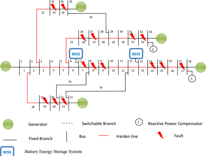

  

  Post-event scenario in enhanced IEEE 33 bus distribution test system for case 4

  Table 8 Resilience for enhanced IEEE 33 bus system with and without action for case 3

  Figure 11 represents a graph of the resilience of different fault scenarios with pre- and post-event resilience enhancements. The x-axis represents different cases and, the y-axis represents resilience value. The blue color column represents the resilience of the system without taking action, red color column represents the resilience of the system after taking immediate action (real-time action), and the green color column represents the resilience of the system after taking second-level action.

  Fig. 11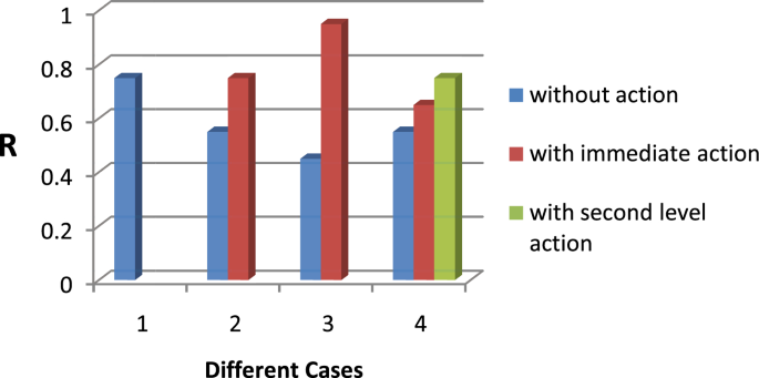

  

  Resilience in four cases with pre- and post-resilience enhancement for enhanced IEEE 33 bus system

4.2 The modified IEEE 69 bus test distribution network

This section serves as a further demonstration of the proposed resilience enhancement strategy. Thus, a larger and well-known IEEE 69 bus distribution system is selected with some modifications, which includes five diesel generators and two BESS. The details of the system are given in Table 9 [39]. A total of 29 lines are hardened in this system. The number of lines, cables and distance between buses is assumed to be the same as discussed for the IEEE 33 bus system. It is also assumed that this distribution system is installed with one feeder (conventional generation) of 4 MW, five DG and two BESS.

Table 9 System description for modified IEEE 69 bus system

• Case 1: Normal operation without fault

  In this scenario, the system is operating under normal conditions. All DERs are functioning correctly, and out of 68 lines in the network, 29 have been hardened. The hardening of power lines is found to be 0.42647, indicating a significant proportion of the lines have been reinforced to withstand potential disturbances. Each DG in the system has a capacity of 100 L, ensuring a substantial energy reserve. The availability of energy resources is 0.2800; as all DG is actively working and so the diesel availability is reduced, Furthermore, the critical load sustainability is measured at 0.9875, which signifies a high level of assurance in sustaining critical loads. Likewise, all the parameters are calculated and fed to RSOM, and resilience is found to be 0.75, as shown in Table 10, which is equal to the set threshold value, so no corrective action will be taken.

  Table 10 Resilience for modified IEEE 69 bus system under normal operating condition without fault for case 1

• Case 2: With faults and resilience smaller than the threshold value after the event

  Different cases are formed according to the nature of faults; one case has been chosen having severe faults that damages many power lines. In this scenario, several faults are considered to have occurred on branches 29, 33, 34, 43, 46, 59 and 60, resulting in the disconnection of one DG and certain branches (59–68 and 28–35) from the main supply, as shown in Fig. 12. After the faults, only 24 hardened lines remained active out of the initial network, with a line hardening parameter of 0.352941. The parameter indicating geographic diversity is found to be 0.6713. The generators are spread geographically throughout the power system network. The reliability of assets is found to be 0.67861, and the path redundancy is found to be 0.0686. These parameters, along with others, are calculated and fed into the RSOM tool, and resilience is found to be 0.65, which falls below the threshold value.

  Fig. 12

  

  Post-event scenario for modified IEEE 69 Bus system after fault for case 2

  Therefore, to improve the system’s resilience, real-time action is needed. Thus, a tie line switch is connected, and the BESS is switched on. Further calculations are made for each parameter. The line hardening is found to increase by 12.49% as three more hardened lines are activated. The path redundancy increases to 0.1205 because connecting the BESS provides multiple paths from the generator to critical loads. Additionally, the reliability of assets by 6.5%. Similarly, all parameters are recalculated and fed into the RSOM. The resilience is found to be 0.85, which is greater than the threshold value. Therefore, any further action is deemed unnecessary.

  The values of the input parameters are shown in Table 11 for the faulted system as well as after the corrective action was taken. From this table, it can be verified that once the corrective action of connecting the tie line and BESS is done, the resilience parameters have improved, leading to the system’s resilience improvement.

  Table 11 Resilience for modified IEEE 69 bus system with and without action for case 2

4.3 Statistical analysis

So far, the analysis has focused on evaluating the effectiveness of the methodology within the context of a predefined threshold value of ${\mathbb{R}}$. Given that resilience revolves around the notion of adequately preparing for and mitigating the impact of worst-case scenarios, we have extended our examination to assess the statistical performance of the proposed methodology across various event and outage scenarios.

In essence, we employ Monte Carlo simulation techniques to generate a spectrum of potential branch damage scenarios. Subsequently, we quantify the resilience of the system under each scenario. Specifically, we generated 1000 scenarios to validate four distinct cases discussed in the methodology Sect. 4.1 for enhanced 33 bus system.

In the Fig. 13, the x-axis represents various fault damage scenarios and the y-axis represents the number of faults (or branches damaged). These 1000 scenarios seem to be sufficient to validate and identify the various cases. In this figure the blue dot symbolizing a lower number of faults, seems to be representing Case 1, which has less catastrophic effect. As the fault count increases and reaches around 8, it transitions to yellow dots, as expected indicating Case 2, having a higher adverse effect on the system compared to the Case 1 category events. Moving further along the fault spectrum, with faults typically falling within the range of 8 to 14, can be categorized under the third category represented by green dots, Case 3, having much more catastrophic effect compared to the Case 1 and Case 2 scenarios. Lastly, occurrence of larger number of faults, from 15 to 20, are depicted by orange dots, seems to be representing Case 4, the group that represents most extreme events. This color-coded representation visually illustrates the progressive categorization of resilience ${\mathbb{R}}$ as they escalate in severity.

Fig. 13

Resilience assessment index based on branch damage scenarios for different event severities

The categorization of the ${\mathbb{R}}$ in the figure seems to be aligned with the observed distribution. The categorization of resilience in the figure reflects the observed distribution of fault occurrences across different scenarios. As depicted in the figure, each color dot corresponds to a specific ${\mathbb{R}}$ and is indicative of different strategies. By examining the positioning of the dots within the figure, we can infer how ${\mathbb{R}}$ is categorized based on their severity. This visual representation helps in understanding how various resilience strategies perform under different fault scenarios, providing valuable insights into the effectiveness of proposed approach.

4.4 Sensitivity analysis

In this paper, the Spearman correlation coefficient analysis was employed to determine the global sensitivity of eight variables within the studied process. The analysis was specifically aimed at qualitatively determining the relative importance of each parameter [41, 42]. The experimental data, conveniently organized in a tabular format, is essential for evaluating parameter behavior and its impact on the process outcomes. The primary objective of the study is to identify which parameters exerted the most and least influence on the observed outcomes, thereby facilitating a deeper understanding of the process dynamics. Notably, the variable that attains the highest value among the eight variables signifies its substantial contribution to the quantification and potential enhancement strategy of the process. Table 12 presents the input parameter values corresponding to different operating scenarios of the distribution system and their sensitivity (spearman coefficient, ρ).

Table 12 Spearman correlation coefficient analysis for eight different parameters

Upon scrutiny of the table, it becomes evident that “critical load sustainability” (R^L) emerged with the highest value (i.e., 0.9256) among all variables, thus highlighting its significance as the most substantial variable in the context of the studied process. This insight emphasizes the importance of prioritizing interventions or optimizations related to this particular parameter for enhancing overall process performance.

5 Conclusion

This paper emphasizes the urgent need to strengthen power system resilience in light of the escalating occurrence of extreme weather events globally. Traditional methods of reliability assessment, reliance on historical data, prove inadequate when confronting HILF events. The introduction of a SOM-based resilience quantification method marks a pivotal advancement, facilitating real-time resilience assessment devoid of historical data. The resilience quantification method is based on only operating condition of the system. Once trained, this RSOM is capable of determining the resilience of any system in no time and hence this quantification tool is used for real-time resilience evaluation and improvement in this paper. The resilience improvement strategy makes use of the real-time quantification method and using this tool the resilience of a distribution system under extreme event is evaluated and based on the resilience value a two-stage resilience improvement strategy is invoked. The first stage is fast and takes immediate action to improve the system resilience by incorporating actions like switching tie lines, connecting local resources like BESS etc. to supply critical loads during extreme event. After taking the first level of action the resilience is again evaluated for the system and based on this value second level of action, which are a little slower, are invoked. As the resilience quantification as well as first level of control action both are very fast, it is considered that these two steps are completed in real-time.

This paper’s important contribution lies in creating a fast and effective methodology that accounts for diverse system factors influencing critical load survivability during extreme events. Moreover, the proposed resilience enhancement strategy pioneers a fresh approach to real-time operation, empowering proactive resilience improvement amid catastrophic events. In contrast to prior studies that centered on resource-constrained methods, this paper introduces a complete framework for the resilient operation of power distribution systems. Statistical and sensitivity analysis on the IEEE 33 bus and 69 bus distribution systems correlates well with the effectiveness of the proposed methodology and manifests substantial enhancements in the system resilience.

In the future, the work can be extended to explore parallels between transportation and power networks, which promises valuable insights into resilience quantification and enhancement through the integration of electric vehicles (EVs), mobile energy resources (MERs) and repair crews.

In sum, this research emphasizes the imperative of adapting power system resilience assessment and management strategies to confront the evolving challenges posed by extreme weather events. It lays a strong foundation for development of a more resilient and adaptive power infrastructure, capable of handling uncertainty and adversity.

References

Younesi A, Shayeghi H, Safari A, Siano P (2020) Assessing the resilience of multi microgrid based widespread power systems against natural disasters using Monte Carlo Simulation. Energy 207:118220. https://doi.org/10.1016/j.energy.2020.118220
Surging weather-related power outages. In: Surging Weather-related Power Outages, Climate Central. https://www.climatecentral.org/climate-matters/surging-weather-related-power-outages. Accessed 22 Feb 2024
Amirioun MH, Aminifar F, Lesani H, Shahidehpour M (2019) Metrics and quantitative framework for assessing microgrid resilience against windstorms. Int J Electr Power Energy Syst 104:716–723. https://doi.org/10.1016/j.ijepes.2018.07.025
Vugrin E, Castillo A, Silva-Monroy C (2017) Resilience metrics for the electric power system: a performance-based approach. Sandia Natl Lab (SNL-NM), Albuquerque, NM (United States). https://doi.org/10.2172/1367499
(2017) Enhancing the resilience of the nation’s electricity system. Natl Academies of Sci Eng and Med. https://doi.org/10.17226/24836
Bhusal N, Abdelmalak M, Kamruzzaman M, Benidris M (2020) Power system resilience: current practices, challenges, and future directions. IEEE Access 8:18064–18086. https://doi.org/10.1109/access.2020.2968586
Campbell RJ (2012a) Weather-related power outages and Electric System resiliency. Congressional Research Service, Library of Congress, Washington, DC
Loveland T, Mahmood R, Patel-Weynand T et al (2012a) National climate assessment technical report on the impacts of climate and land use and land cover change. Open-File Report i-86. https://doi.org/10.3133/ofr20121155
Sanstad A, Zhu Q, Leibowicz B et al (2020) Case studies of the economic impacts of power interruptions and damage to electricity system infrastructure from extreme events. https://doi.org/10.2172/1725813
Hotchkiss EL, Dane A (2019) Resilience roadmap: a collaborative approach to multijurisdictional resilience planning. No. NREL/TP-6A20-73509. National Renewable Energy Laboratory (NREL), Golden, CO (United States). https://doi.org/10.2172/1530716
Cutter, Susan L et al (2013) Disaster resilience: a national imperative. Environ Sci Policy Sustain Dev 55(2):25–29
Panteli M, Mancarella P, Trakas DN et al (2017) Metrics and quantification of operational and infrastructure resilience in power systems. IEEE Trans Power Syst 32:4732–4742. https://doi.org/10.1109/tpwrs.2017.2664141
Lee SM, Chinthavali S, Bhusal N et al (2024) Quantifying the power system resilience of the US power grid through weather and power outage data mapping. IEEE Access 12:5237–5255. https://doi.org/10.1109/access.2023.3347129
Petit FDP, Bassett GW, Black R et al (2013) Resilience measurement index: an indicator of critical infrastructure resilience. No. ANL/DIS-13-01. Argonne National Lab. (ANL), Argonne, IL (United States). https://doi.org/10.2172/1087819
Panteli M, Trakas DN, Mancarella P, Hatziargyriou ND (2016) Boosting the power grid resilience to extreme weather events using defensive islanding. IEEE Trans Smart Grid 7:2913–2922. https://doi.org/10.1109/tsg.2016.2535228
Kwasinski A (2016) Quantitative model and metrics of electrical grids’ resilience evaluated at a power distribution level. Energies 9:93. https://doi.org/10.3390/en9020093
Anderson K, Li X, Dalvi S et al (2021) Integrating the value of electricity resilience in energy planning and operations decisions. IEEE Syst J 15:204–214. https://doi.org/10.1109/jsyst.2019.2961298
Lv C, Yu H, Li P et al (2020) Coordinated operation and planning of integrated electricity and gas community energy system with enhanced operational resilience. IEEE Access 8:59257–59277. https://doi.org/10.1109/access.2020.2982412
Ghosh P, De M (2021) Impact of microgrid towards power system resilience improvement during extreme events. In: 2021 International conference on computational performance evaluation (ComPE). https://doi.org/10.1109/compe53109.2021.9752302
Ghorbani E, Hajiabadi ME, Samadi M, Lotfi H (2023) Providing a preventive maintenance strategy for enhancing distribution network resilience based on cost–benefit analysis. Electr Eng 105:979–991. https://doi.org/10.1007/s00202-022-01710-5
Mondal S, Ghosh P, De M (2024) Evaluating the impact of coordinated multiple mobile emergency resources on distribution system resilience improvement. Sustain Energy Grids Netw 38:101252. https://doi.org/10.1016/j.segan.2023.101252
Hosseinzadeh A, Zakariazadeh A (2022) Enhancing the resilience of distribution systems through optimal restoration of sensitive loads based on hybrid network zoning. Electr Eng 105:745–760. https://doi.org/10.1007/s00202-022-01695-1
Ildarabadi R, Lotfi H, Hajiabadi ME, Nikkhah MH (2023) Presenting a new mathematical modeling for distribution network resilience based on the optimal construction of tie-lines considering importance of critical electrical loads. Electr Eng. https://doi.org/10.1007/s00202-023-02077-x
Utkarsh K, Ding F (2022) Self-organizing map-based resilience quantification and resilient control of distribution systems under extreme events. IEEE Trans Smart Grid 13:1923–1937. https://doi.org/10.1109/tsg.2022.3150226
Mahzarnia M, Moghaddam MP, Baboli PT, Siano P (2020) A review of the measures to enhance power systems resilience. IEEE Syst J 14:4059–4070. https://doi.org/10.1109/jsyst.2020.2965993
Arjomandi-Nezhad A, Fotuhi-Firuzabad M, Moeini-Aghtaie M et al (2021) Modeling and optimizing recovery strategies for power distribution system resilience. IEEE Syst J 15:4725–4734. https://doi.org/10.1109/jsyst.2020.3020058
Mahdavi M, Javadi MS, Wang F, Catalao JP (2022) An efficient model for accurate evaluation of consumption pattern in distribution system reconfiguration. IEEE Trans Ind Appl 58:3102–3111. https://doi.org/10.1109/tia.2022.3148061
Mahdavi M, Alhelou HH, Siano P, Loia V (2022) Robust mixed-integer programing model for reconfiguration of distribution feeders under uncertain and variable loads considering capacitor banks, voltage regulators, and protective relays. IEEE Trans Ind Inf 18:7790–7803. https://doi.org/10.1109/tii.2022.3141412
Huang G, Wang J, Chen C et al (2017) Integration of preventive and emergency responses for power grid resilience enhancement. IEEE Trans Power Syst 32:4451–4463. https://doi.org/10.1109/tpwrs.2017.2685640
Morshedlou N, Barker K, Sansavini G (2019) Restorative capacity optimization for complex infrastructure networks. IEEE Syst J 13:2559–2569. https://doi.org/10.1109/jsyst.2019.2915930
Ghasemi S, Darwesh A, Moshtagh J (2023) Critical loads restoration of distribution networks after blackout by microgrids to improve network resiliency. Electr Eng 105:2909–2922. https://doi.org/10.1007/s00202-023-01832-4
Kohonen T (1990) The self-organizing map https://doi.org/10.1109/5.58325.
Willis HH (2015) Measuring the resilience of energy distribution systems. RAND Corporation
Jeffers RF, Staid A, Baca MJ et al (2018) Analysis of microgrid locations benefitting community resilience for Puerto Rico. No. SAND-2018-11145. Sandia National Lab. (SNL-NM), Albuquerque, NM (United States). https://doi.org/10.2172/1481633
In: Managing aging distribution systems assets, available at https://restservice.epri.com/publicdownload/ 000000000001000422/0/Product. Accessed 11 Nov 2023
In: Diesel generator fuel consumption chart in litres—FW power. https://fwpower.co.uk/wp-content/uploads/2018/12/Diesel-Generator-Fuel-Consumption-Chart-in-Litres.pdf. Accessed 14 Nov 2023
Florent F, LebbahM ,Azzag H, Lacaille J (2020) A Survey and Implementation of Performance Metrics for Self-Organized Maps. https://doi.org/10.48550/arXiv.2011.05847.
Dolatabadi SH, Ghorbanian M, Siano P, Hatziargyriou ND (2021) An enhanced IEEE 33 bus benchmark test system for distribution system studies. IEEE Trans Power Syst 36:2565–2572. https://doi.org/10.1109/tpwrs.2020.3038030
Oboudi MH, Mohammadi M, Rastegar M (2019) Resilience-oriented intentional islanding of reconfigurable distribution power systems. J Modern Power Syst Clean Energy 7:741–752. https://doi.org/10.1007/s40565-019-0567-9
Luo D, Xia Y, Zeng Y et al (2018) Evaluation method of distribution network resilience focusing on critical loads. IEEE Access 6:61633–61639. https://doi.org/10.1109/access.2018.2872941
Biswas K, Rahman MT, Almulihi AH, Alassery F, Al Askary MAH, Hai TB, Kabir SS, Khan AI, Ahmed R (2022) Uncertainty handling in wellbore trajectory design: a modified cellular spotted hyena optimizer-based approach. J Petrol Explor Prod Technol 12(10):2643–2661
Biswas K, Nazir A, Rahman MT, Khandaker MU, Idris AM, Islam J, Rahman MA, Jallad AHM (2022) A hybrid multi objective cellular spotted hyena optimizer for wellbore trajectory optimization. PLoS ONE 17(1):e0261427
Author information
Authors and Affiliations
Contributions
Roshan Kumar contributed to conceptualization, investigation and writing—original draft. Mala De was involved in conceptualization, investigation, supervision, writing—review and editing and investigation.
Corresponding author
Ethics declarations
Conflict of interest
The authors declare no competing interests.
Additional information
Publisher’s Note
Springer Nature remains neutral with regard to jurisdictional claims in published maps and institutional affiliations.
Rights and permissions
Springer Nature or its licensor (e.g. a society or other partner) holds exclusive rights to this article under a publishing agreement with the author(s) or other rightsholder(s); author self-archiving of the accepted manuscript version of this article is solely governed by the terms of such publishing agreement and applicable law.
About this article
Cite this article
Kumar, R., De, M. Power system resilience quantification and enhancement strategy for real-time operation. Electr Eng (2024). https://doi.org/10.1007/s00202-024-02350-7
Received:
Accepted:
Published:
DOI: https://doi.org/10.1007/s00202-024-02350-7