
Abstract
We study an interactive framework that explicitly allows for nonrational behavior. We do not place any restrictions on how players’ behavior deviates from rationality, but rather, on players’ higher-order beliefs about the frequency of such deviations. We assume that there exists a probability p such that all players believe, with at least probability p, that their opponents play rationally. This, together with the assumption of a common prior, leads to what we call the set of p-rational outcomes, which we define and characterize for arbitrary probability p. We then show that this set varies continuously in p and converges to the set of correlated equilibria as p approaches 1, thus establishing robustness of the correlated equilibrium concept to relaxing rationality and common knowledge of rationality. The p-rational outcomes are easy to compute, also for games of incomplete information. Importantly, they can be applied to observed frequencies of play for arbitrary normal-form games to derive a measure of rationality \(\overline{p}\) that bounds from below the probability with which any given player chooses actions consistent with payoff maximization and common knowledge of payoff maximization.
1 Introduction
Rationality, understood as consistency of behavior with stated objectives, information, and strategies available, naturally lies at the heart of game theory. Still today, most of game theory and its applications takes the rationality of the agents, knowledge and higher knowledge thereof as given and, in an important way, relies on these to make (ideally robust) predictions about behavior. However, it is clear that, in practice, departures from full consistency or rationality not only occur and occur often, but they also occur in innumerable ways.Footnote 1 To address this, we develop a theory that relaxes the assumption of rationality and higher order knowledge of rationality. We assume that for any given probability \(p\in [0,1]\), players choose rationally with probability at least p and with respect to beliefs that assign probability at least p to their opponents’ choosing rationally as well; we put no constraint on what the remaining actions or action profiles (occurring with frequency at most \(1-p\)) may be. Among other things, we study the robustness of behavior with respect to p, that is, its sensitivity to the introduction of nonrationality, and derive a measure of “rationality” for observed frequencies of play.
As a brief illustration, consider the following two examples. The first is a stylized penalty kick game, taken from Palacios-Huerta (2003), based on actual penalty kicks shot by professional soccer players in European leagues between 1995 and 2000.Footnote 2 Players’ strategies are reduced to kick left or right (KL, KR) for the kicker (row player) and to jump left or right (JL, JR) for the goalkeeper (column player). The payoffs are described in Fig. 1 in the first matrix (and correspond to probability of scoring for the kicker and probability of saving for the goalkeeper), the second matrix describes the empirical frequencies with which the different strategies were played in the field, and the third presents the probabilities assigned to each outcome by the unique Nash equilibrium distribution of the game.

Penalty kicks in professional European soccer leagues (\(\overline{p}\approx 0.96\))
Although close, it can be checked that, if one assumes the existence of a common prior, strictly speaking, frequencies of play are inconsistent with common knowledge of rationality, as players are not playing best-responses to one another. As we will discuss in Sect. 5, where we introduce an empirical measure of rationality derived from our theory that allows to quantify discrepancies from equilibrium play, we compute that at least 96 % of each player’s (row player’s and column player’s) actions are consistent with payoff maximization and common knowledge of payoff maximization.

Kreps game (\(\overline{p} \approx 0.7\))
The second example, represented in Fig. 2, is a game taken from Goeree and Holt (2001) and due to David Kreps that has three Nash equilibria. Here subjects playing the column role typically choose strategy (NN) that is the only strategy that is not in the support of any of the Nash equilibria of the game. Nonetheless, according to our measure, at least 70 % of each player’s (row player’s and column player’s) actions are consistent with payoff-maximization and common knowledge of payoff maximization, whether or not the common prior assumption holds.
In this paper, we are interested in a theory of strategic interaction that incorporates the following two aspects of bounded rationality: (i) some (possibly small) amount of nonrational behavior, and (ii) the capacity of players to expect, and optimally react, to nonrational behavior by their opponents. In order to develop such a theory, we relax the assumptions that agents are rational at all times and that there is common knowledge of rationality. We replace these with a substantially weaker assumption, namely, that there exists a lower bound on the probability that players assign to their opponents being rational, that is, to choosing actions that are payoff-maximizing given their own information. More specifically, we study the behavior that arises, if, in every state of the world, each player believes that the other players are rational with a probability p or more. This is what we call common knowledge of mutual p-belief in opponents’ rationality. Together with the existence of a common prior it defines the notion of p-rational outcome, which is at the center of our paper. Thus characterizing the set of p-rational outcomes is tantamount to characterizing behavior that allows for mistakes, arbitrary mistakes, and optimization w.r.t. the possibility of mistakes, as long as the expected frequency of mistakes by others is bounded above by \(1-p\). Importantly, we put no restriction on what it means to be non-rational, except that the rules of the game implicitly require agents to select some action from the action space.Footnote 3
After defining our central notion of p-rational outcomes, we give a strategic characterization in Theorem 1 in terms of what we call (X, p)-correlated equilibria. These are correlated equilibria, where incentive constraints hold on a subset (\(X\subseteq A\)) of the overall action space, and where actions from this subset are believed to be played with certain minimum probability p. The theorem provides a nonepistemic characterization that uses the (X, p)-correlated equilibria to relate the p-rational outcomes to correlated equilibria and can be seen as giving a generalization that extends the main result by Aumann (1987) to contexts of bounded rationality. The set of p-rational outcomes is described by linear inequalities consisting of incentive and p-belief constraints, and for any p; it always contains the set of correlated equilibria, with which it coincides when \(p=1\). When \(p=0\), the set of p-rational outcomes makes up the whole space of distributions over action space A, \(\Delta (A)\).
In Theorem 2, we show that, besides being nonempty, convex and compact, the set of p-rational outcomes varies continuously in the underlying parameter p. We further show that when p is sufficiently close to 1, then rationalizable strategy profiles are played with probability at least p. These results confirm in some sense the robustness of the correlated equilibrium concept to bounded rationality. Proposition 2 further characterizes the p-rational equilibria as Bayesian Nash equilibria of incomplete information games, namely certain “canonical elaborations” as defined in Kajii and Morris (1997a, (1997b), that are perturbations of the underlying (complete information) game G with some restrictions on the frequencies of “standard” and “committed” types. The proposition can be seen as also providing an epistemic foundation of Bayesian equilibria of such perturbed games with “standard” and “committed” types.
Theorem 4 then shows that our main characterization result extends directly to the case of games of incomplete information using the notion of Bayes correlated equilibrium of Bergemann and Morris (2015). To the extent that their results show robustness of the Bayes correlated equilibria to underlying private information structures, we can view our results as showing that the p-rational Bayes outcomes we characterize (which coincide with the Bayes correlated equilibria when \(p=1\)) are robust to nonrational behavior by the players, provided it occurs with probability no more than \(1-p\).
As a further application of our theory, we use the p-rational outcomes to derive a unique number \(\overline{p} \in [0,1]\) that quantifies proximity to common knowledge of rationality in a normal-form strategic interaction. In interactions where the common prior assumption can be expected to hold, for any given distribution of play, say \(\pi \in \Delta (A)\), we can define a unique number \(\overline{p} \in [0,1]\), that gives the largest p such that each player plays actions that are consistent with common knowledge of payoff maximization given \(\pi \) with frequency at least p. This gives a direct measure of the maximum possible amount of actions consistent with payoff maximization reflected in the distribution \(\pi \). For interactions, where the common prior assumption does not hold, then players may be acting rationally, but their rationality is underestimated by \(\overline{p}\) as it does not take into account possible inconsistencies in beliefs. Allowing for this, one can show that \(\overline{p}\) is a lower bound for the maximum possible amount of actions consistent with payoff maximization and common knowledge of payoff maximization, reflected in the distribution \(\pi \). Therefore, the value \(\overline{p}\) can be useful as a measure of minimum amount of rationality in experimental data, whether or not there is a common prior. We discuss this in more detail Sect. 5.
At a theoretical level, our analysis builds on the epistemic literature, centered around the concepts of rationalizability, Bernheim (1984) and Pearce (1984), and correlated equilibrium, Aumann (1974), Aumann (1987), that characterizes behavior under varying assumptions on players’ rationality and their reciprocal beliefs in each others’ rationality. Tan and da Costa Werlang (1988) show that independent rationalizability characterizes rationality and common certainty of rationality; and Brandenburger and Dekel (1987) connect it to subjective correlated equilibria and correlated rationalizability. Using the notion of common p-belief (of Monderer and Samet (1989), who introduce the concept to study robustness of equilibria to incomplete information regarding payoffs, and thus, do not account for deviations from rationality), Hu (2007) introduces the notion of (correlated) p-rationalizability, and shows that it characterizes rationality and common p-belief in rationality, for general \(p \le 1\).Footnote 4 He also shows that as p converges to 1, the set of p-rationalizable actions approaches the set of rationalizable actions.
For incomplete information games and within an ex ante context, Forges (1993) and Forges (2006) introduces several notions of correlated equilibrium. Lehrer et al. (2010), Lehrer et al. (2013) clarify epistemically the role of different assumptions and information structures and study their effect on equilibrium behavior. Bergemann and Morris (2015) introduce a further broader notion of correlated equilibrium, which they call Bayes correlated equilibrium, and which they show characterizes behavior robust to varying information structures. Bayes correlated equilibrium is the equilibrium notion we use for our incomplete information analysis. At the interim stage, starting from hierarchies of beliefs, Dekel et al. (2007) introduce the notion interim correlated rationalizability and show that it characterizes common certainty of rationality. Germano et al. (2016), introduce the notion of interim correlated p-rationalizability, and show that it characterizes common p-belief in rationality, for general \(p \le 1\). We view the ex ante and the interim approaches as providing complementary results; the ex ante approach used in this paper making epistemically speaking more restrictive assumptions (assuming besides a common prior also common knowledge of the model and the epistemic assumptions it entails). To the extent that the additional assumptions are satisfied, the ex ante approach provides an effective tool for characterizing resulting behavior and, in our case, also yields sharper bounds and predictions as compared to the notions of p-rationalizability or interim correlated p-rationalizability.
The paper is structured as follows. Section 2 sets up both the game-theoretic and epistemic framework and recalls and discusses the main results by Aumann (1987). Section 3 is the main section, which introduces the notion of p-rational outcome and contains strategic and topological characterizations, as well as some simple examples. Section 4 contains some extensions, including to games of incomplete information. Section 5 shows how the theory implies a natural measure to quantify the degree of “rational” behavior in strategic interactions, and Sect. 6 provides some concluding remarks. All the proofs are in the Appendix.
2 Preliminaries
In this section, we recall some well-known concepts in game theory and epistemic game theory needed for the analysis of Sect. 3. In Sect. 2.1, we present the game-theoretic framework and the standard solution concepts later generalized: correlated and subjective correlated equilibrium (Aumann 1974). Then, in Sect. 2.2, we introduce the epistemic framework, in which interactive knowledge and beliefs are formalized; this uses standard constructions by Aumann (1987), Brandenburger and Dekel (1987) or Monderer and Samet (1989), among others. Finally, in Sect. 2.3, we discuss the main result by Aumann (1987), which relates common knowledge assumptions regarding rationality with correlated and subjective correlated equilibria.
2.1 Correlated equilibria
A (finite, normal-form) game is defined as a tuple \(G=\left\langle I,\left( A_{i}\right) _{i\in I},\left( u_{i}\right) _{i\in I}\right\rangle \), where I is a finite set of players, and for any player i we have: a finite set of actions \(A_i\) and a payoff function \(u_{i}:A\rightarrow \mathbb {R}\), where \(A=\prod _{i\in I}A_{i}\) denotes the set of action profiles. Given distribution \(\pi \in \Delta (A)\), for any player i, we say that action \(a_{i}\) is optimal w.r.t. \(\pi \) if,
where \(A_{-i}=\prod _{j\ne i}A_{j}\). Then, following Aumann (1974): (i) a distribution \(\pi \in \Delta (A)\) is a correlated equilibrium if for any player i every action \(a_{i}\) is optimal w.r.t. \(\pi \), and (ii) a family of distributions \((\pi _{i})_{i\in I}\subseteq \Delta (A)\) is a subjective correlated equilibrium if for any player i every action \(a_{i}\) is optimal w.r.t. \(\pi _{i}\). We denote the sets of correlated equilibria and subjective correlated equilibria of G by \(CE\left( G\right) \) and SCE(G), respectively. It follows by definition that \((CE(G))^{I}\subseteq SCE(G)\). It is easy to see that every Nash equilibrium induces a correlated equilibrium; thus, CE(G) and SCE(G) are both nonempty.
2.2 Epistemic framework
Interactive knowledge and beliefs are exogenously modeled by a belief system, which consists of a list \(B=\left\langle \Omega ,\left( \Pi _{i}\right) _{i\in I},\left( \alpha _{i}\right) _{i\in I},(\mu _{i})_{i\in I}\right\rangle \), where \(\Omega \) is a finite set of states (of the world), and for each player i we have: (i) \(\Pi _{i}\), a knowledge partition of \(\Omega \), where for any state \(\omega \) we denote the cell containing \(\omega \) by \(\Pi _{i}\left( \omega \right) \), (ii) a strategy map \(\alpha _{i}:\Omega \rightarrow A_{i}\) measurable w.r.t. \(\Pi _{i}\), and (iii) a (subjective) prior belief \(\mu _{i}\in \Delta \left( \Omega \right) \) with full support. An event is a collection of states \(E \subseteq \Omega \). As mentioned above, belief systems formalize the following two epistemic aspects:
-
(1)
Interim knowledge For any player i and any state \(\omega \), player i’s knowledge at \(\omega \) is represented by \(\Pi _{i}\left( \omega \right) \): we say player i knows event E at state \(\omega \) if \(\Pi _{i}\left( \omega \right) \subseteq E\). Player i’s knowledge operator is thus defined as follows,
$$\begin{aligned} E\mapsto K_{i}\left( E\right) =\left\{ \omega \in \Omega \left| \Pi _{i}\left( \omega \right) \subseteq E\right. \right\} ,\,\text { for any }\,E\subseteq \Omega . \end{aligned}$$Note that the measurability of the strategy maps implies that each player knows at every state what action she chooses. We say that an event E is evident knowledge if \(E\subseteq \bigcap _{i\in I}K_{i}\left( E\right) \), and for state \(\omega \), event C is commonly known at \(\omega \) if there exists some evident knowledge E such that \(\omega \in E\subseteq \bigcap _{i\in I}K_{i}\left( E\right) \). We denote the event that C is commonly known by CK(C).
-
(2)
Interim beliefs For each player i knowledge partition \(\Pi _{i}\) and prior belief \(\mu _{i}\) induce interim beliefs at each state \(\omega \),
$$\begin{aligned} \mu _{i}(\omega )[E]= \frac{\mu _{i}\left[ E\cap \Pi _{i}\left( \omega \right) \right] }{\mu _{i}\left[ \Pi _{i}\left( \omega \right) \right] },\quad \text { for any }\,E\subseteq \Omega . \end{aligned}$$Then, following Monderer and Samet (1989), for any probability \(p\in [0,1]\) we say that player i p-believes event E at state \(\omega \) if \(\mu _{i}(\omega )[E]\ge p\). Player i’s p-belief operator is thus defined as follows,
$$\begin{aligned} E\mapsto B_{i}^{p}\left( E\right) =\left\{ \omega \in \Omega \left| \mu _{i}(\omega )[E]\ge p\right. \right\} ,\quad \text { for any }\,E\subseteq \Omega . \end{aligned}$$We say that an event E is p-evident belief if \(E\subseteq \bigcap _{i\in I}B_{i}^{p}\left( E\right) \), and for state \(\omega \), event C is common p-belief at \(\omega \) if there exists some p-evident belief E such that \(\omega \in E\subseteq \bigcap _{i\in I}B_{i}^{p}\left( E\right) \). We denote the event that C is common p-belief by \(CB^{p}(C)\). It is easy to see that in this framework, knowledge and 1-belief coincide, due to the fact that prior beliefs have full support.
2.3 Correlated equilibria as an expression of Bayesian rationality
Each belief system B induces, for each player i, the following interim beliefs on her opponents’ behavior at each state \(\omega \): \(\mu _{i}(\omega )[a_{-i}]=\mu _{i}(\omega )[\bigcap _{j\ne i}\alpha _{j}^{-1}(a_{j})]\) for any \(a_{-i}\in A_{-i}\), and thus, the following interim expected payoff,
for each \(a_{i}\in A_{i}\). Then, we say that player i is (Bayesian) rational at state \(\omega \) if her choice is optimal w.r.t. her interim beliefs, i.e., if \(\alpha _{i}(\omega )\in \text {argmax}_{a_{i}\in A_{i}}\mathbb {E}_{B}(\omega )\left[ u_{i}\left( \alpha _{-i};a_{i}\right) \right] \), and denote the event that player i is rational by \(R_{i}\). We denote the event that every player is rational by R. Finally, note that belief system B also induces, for each player i, a subjective outcome (distribution) \(\pi ^{B}_{i}\in \Delta (A)\) given by \(\pi ^{B}_{i}(a)=\mu _{i}[\bigcap _{j\in I}\alpha _{j}^{-1}(a_{j})]\) for any \(a\in A\). Aumann (1987) studies the impact of the following two properties in belief systems:
-
Common knowledge of rationality Belief system B is rational if players are rational at every state, i.e., if \(\Omega =R\). Note that since \(\Omega \) is evident knowledge, it follows that rationality is commonly known at every state. Aumann (1987) shows that if belief system B is rational, then the family of subjective outcomes it induces is a subjective correlated equilibrium: \((\pi ^{B}_{i})_{i\in I}\in SCE(G)\).
-
Common prior assumption Belief system B satisfies the common prior assumption if all the players hold the same prior belief, i.e., if \(\mu _{i}=\mu _{j}\) for any \(i,j\in I\). In case the common prior assumption is satisfied, we drop subscripts and denote the common prior belief, to which we refer as the common prior, by simply \(\mu \). In this case, B induces an objective outcome (distribution) \(\pi ^{B}\in \Delta (A)\) given by \(\pi ^{B}(a)=\mu [\bigcap _{i\in I}\alpha _{i}^{-1}(a_{i})]\) for any \(a\in A\).Footnote 5 The main result in Aumann (1987) shows that if B is rational and satisfies the common prior assumption, then the objective outcome it induces is a correlated equilibrium: \(\pi ^{B}\in CE(G)\).
Two aspects of the formalization of belief systems are crucial for obtaining equilibrium behavior: (i) strategy maps \((\alpha _{i})_{i\in I}\) are structurally commonly known,Footnote 6 and (ii) the common prior assumption implies that players hold correct beliefs about how information is distributed among their opponents.Footnote 7 The combination of this features yields that players hold, indeed, correct beliefs about how their opponents play, since: they hold correct beliefs about how information is distributed and they hold correct beliefs about how, specifically, choice is made contingent on information. For examples of epistemic frameworks that offer a more transparent distinction between equilibrium assumptions (as the two mentioned) and common knowledge of rationality see Tan and da Costa Werlang (1988), Dekel et al. (2007) or Battigalli et al. (2011).
3 Bounded rationality and correlated equilibria
In this section we characterize an extension of correlated equilibrium that incorporates the following two aspects of bounded rationality: (i) some (possibly small) amount of nonrational behavior, and (ii) the capacity of players to expect, and optimally react, to nonrational behavior by their opponents. Obviously, such behavior is at odds with common knowledge of rationality: a weaker epistemic assumption is required. In Sect. 3.1, we present our central epistemic assumption, discuss why it stands as a compelling relaxation, and define the probabilistic behavior it induces as p-rational outcomes (Definition 1). It remains unclear whether the p-rational outcomes can be characterized without having to go through a tedious process of epistemic modeling. This problem is solved in Sect. 3.2, where we present an easily computable generalization of correlated equilibria, (X, p)-correlated equilibria, and show in Theorem 1 that the set of p-rational outcomes can be characterized in terms of (X, p)-correlated equilibria of a related game, Aumann and Dreze (2008) doubled game. In Sect. 3.3, we present some examples illustrating the p-rational outcomes, and in Sect. 3.4, we discuss geometric properties of the set of p-rational outcomes, and show that this set is robust to small variations in the amount of nonrational behavior.
3.1 \(\varvec{p}\)-Rational outcomes: epistemic motivation
In order to capture the two features of bounded rationality mentioned above, we need to depart from common knowledge of rationality. A natural and standard way to relax knowledge assumptions is to resort to Monderer and Samet (1989) notion of p-belief, as recalled in Sect. 2.2. However, it is not straightforward how p-beliefs should be applied in order to accommodate the kind of nonrational behavior we are looking for. Thus we propose to substitute common knowledge of rationality with common knowledge of mutual p-belief in opponents’ rationality. That is, we assume that it is commonly known that there exists some probability p for which every player believes, with probability at least p, that the rest of players are rational. This idea is formalized by belief systems that satisfy:
-
Common knowledge of mutual p-belief in opponents’ rationality (MB \(^{\varvec{p}}\) R) For fixed probability p, mutual p-belief in opponents’ rationality holds at every state, i.e., \(\Omega =\bigcap _{i\in I}B_{i}^{p}(R_{-i})\).
Note then that, under common knowledge of mutual p-belief in rationality (MB\(^{p}\)R), we have: (i) some (possibly small) amount of nonrational behavior, and (ii) capacity of players’ to expect, and optimally react, to nonrational behavior by their opponents. Thus, MB\(^{p}\)R captures the two aspects of bounded rationality we are looking to characterize.Footnote 8 Lemma 1 below studies how common knowledge of rationality, common p-belief in rationality, and MB\(^{p}\)R relate to each other, and illustrates some properties of the latter, which motivate its suitability as a relaxation of common knowledge of rationality.
Lemma 1
Let G be a game, p, a positive probability, and B, a belief system. Then:
-
(i)
\(\Omega =CB^{p}(R)\) if and only if \(\Omega =R\).
-
(ii)
If \(p=1\), then \(\Omega =R\) if and only if \(\Omega =\bigcap _{i\in I}B_{i}^{p}(R_{-i})\).
-
(iii)
If B satisfies MB\(^{p}\)R and the common prior assumption, then \(\mu \left[ R_{i}\right] \ge p\) for any player i, and \(\mu \left[ R\right] \ge p^{2}\).
We provide some interpretations. The first result states that assuming common p-belief in rationality at every state is identical to assuming rationality at every state. Thus, for any \(p>0\), behavior induced by common p-belief in rationality corresponds exactly to correlated equilibria, and hence, we can conclude that common p-belief in rationality is not appropriate to capture the aspects of bounded rationality we are interested in. The second result shows that in the limit case of full rationality, when \(p=1\), MB\(^{p}\)R and common knowledge of rationality coincide. Thus, when nonrational behavior is excluded, MB\(^{p}\)R induces precisely, correlated equilibria. The third result studies the impact of the common prior assumption on MB\(^{p}\)R and shows that the fact that the common prior assumption entails correct belief implies that, for fixed p, MB\(^{p}\)R leads toindividual rational behavior with at least probability p, and to collective rational behavior with at least probability \(p^2\), so that collective nonrational behavior is bounded by probability \((1-p^{2})\). Then, we define the outcome distributions induced by belief systems satisfying MB\(^{p}\)R and the common prior assumption as follows:
Definition 1
(p-Rational outcome) Let G be a game, and p, a probability. Then, we say that distribution \(\pi \in \Delta (A)\) is a p-rational outcome if it is induced by some belief system B that satisfies MB\(^{p}\)R and the common prior assumption. We denote the set of p-rational outcomes by p-RO(G).
The interest of p-rational outcomes lies in the notion of bounded rationality that they capture via MB\(^p\)R. Yet, it seems problematic that, given a game G and a probability p, in order to characterize the set of p-rational outcomes, we need to consider all the possible belief systems satisfying MB\(^{p}\)R and the common prior assumption, and then, compute the outcomes they induce. We know that this can be circumvented for rational systems satisfying common knowledge of rationality: by Aumann (1987) theorem, the behavior of these belief systems is captured by the set of correlated equilibria, which is easily computable through certain incentive constraints in the game G. In the next section, we explore whether it is possible to characterize the set of p-rational outcomes without the need of epistemic modeling.
3.2 \(\varvec{p}\)-Rational outcomes: strategic characterization
We are interested in characterizing the set of p-rational outcomes in terms of the original game G, without evoking belief systems. Before doing so we need to first introduce the following notion of (X, p)-correlated equilibrium. This concept generalizes the notion of correlated equilibrium by explicitly allowing for some actions to be played nonoptimally, and plays a key role in our characterization result, Theorem 1 below.
Definition 2
((X, p)-Correlated equilibrium) Let G be a game. Then, for any \(X=\prod _{i\in I}X_{i}\subseteq A\) and any probability p we say that distribution \(\pi \in \Delta \left( A\right) \) is a \(\left( X,p\right) \)-correlated equilibrium if for any player i the following hold:
-
(i)
Incentive constraints For any action \(a_{i}\in X_{i}\), \(a_{i}\in \text {argmax}_{a'_{i}\in A_{i}}\sum _{a_{-i} \in A_{-i}} \pi [\left( a_{-i};a_{i}\right) ]\cdot u_{i}\left( a_{-i};a'_{i}\right) \).
-
(ii)
p-belief constraints For any action \(a_{i}\in A_{i}\), \(\pi \left[ X_{-i}\times \left\{ a_{i}\right\} \right] \ge p\cdot \pi \left[ A_{-i}\times \left\{ a_{i}\right\} \right] \).
We denote the set of \(\left( X,p\right) \)-correlated equilibria of G by \(\left( X,p\right) \)-\(CE\left( G\right) \).
This notion weakens the usual incentive constraints in the following sense. Fix a probability \(p\in [0,1]\) and, for each player i, a subset \(X_{i}\subseteq A_{i}\) such that the distribution on the overall set of action profiles \(\pi \in \Delta (A)\) satisfies two kinds of constraints:
-
(i)
Standard incentive constraints that are not required to hold for all actions, but rather, only for those in \(X_{i}\). Thus, strictly smaller subsets \(X_{i}\subsetneq A_i\) can reflect agents that, for actions in \(A_{i} {\setminus } X_{i}\), follow a mediator’s advice without questioning the “rationality” of doing so (e.g., in the sense of a social norm) or simply act irrationally in the sense of making mistakes (for whatever reason and in whichever way). It is easy to see that, when \(X=A\), the incentive constraints imply that \(\left( A,p\right) - CE\left( G\right) =CE\left( G\right) \) regardless of the value of p.
-
(ii)
The p-belief constraints require that, at the interim level, each player assigns probability at least p to the rest of the players all choosing action profiles from \(X_{-i}=\prod _{j\ne i}X_{j}\). The belief constraints can reflect bounds or statistical regularities with which deviations from “rationality” are roughly known to occur, by restricting the probability of this occurrence to at most \(1-p\). When the possibility of irrational behavior is excluded (\(p=1\)), then we have that \(\left( X,1\right) - CE\left( G\right) \subseteq CE\left( G\right) \) for any \(X\in \prod _{i\in I}2^{A_{i}}\). However, the opposite inclusion fails if \(\pi \) is a correlated equilibrium of G whose support is not included in X (but clearly it holds when \(X=A\)).
Finally, note that the computation of (X, p)-correlated equilibria is similar to that of correlated equilibria; it only involves \(\sum _{i\in I}\left( |X_{i}| \left( |A_{i}|-1\right) +|A_{i}|\right) \le \sum _{i\in I}|A_{i}| \left( |A_{i}|+1\right) \) linear incentive and p-belief constraints. Now, in order to complete our characterization result in Theorem 1 we need to recall the notion of doubled game due to Aumann and Dreze (2008):
Definition 3
(Doubled game, cf.Aumann and Dreze 2008) Let G be a game. Then, the doubled game of G is defined as the tuple \(2G=\left\langle I,\left( A_{i}'\right) _{i\in I},\left( u_{i}'\right) _{i\in I}\right\rangle \), where for each player i:
-
(i)
\(A_{i}'=A_{i}\times \{1,2\}\) is player i’s set of pure actions. With some abuse of notation, we denote a generic element of \(A'=\prod _{i\in I}A_{i}'\) by \(\left( a,\nu \right) \), where, for \(\nu \in \{1,2\}^{I}\), \(\nu _{i}\) specifies which copy of \(A_{i}\) in \(A_{i}'\) player i’s pure action belongs to.
-
(ii)
\(u_{i}':A'\rightarrow \mathbb {R}\), given by \((a,\nu )\mapsto u_{i}\left( a\right) \) is player i’s payoff function,
Thus, in this context, when writing the action spaces of the game 2G as \(A_{i}'=A_{i}\times \{1,2\}\) we mean that for each player there are two copies of the original action space \(A_{i}\), with the same payoffs as in G. Note that any distribution on the action profiles of 2G, \(\hat{\pi }\in \Delta \left( A'\right) \), induces a distribution on the action profiles of G in a natural way by taking the marginal on A, that is, \(\pi =\text {marg}_{A}\hat{\pi }\). For any subset \(Y\subseteq \Delta \left( A'\right) \) we denote \(\mathbf{marg }_{A}(Y)=\bigcup _{\hat{\pi }\in Y}\left\{ \text {marg}_{A}\hat{\pi }\right\} \). These elements provide all the tools required to go on with the characterization of the set of p-rational outcomes of the game G.
Our next theorem shows that these can be expressed in terms of computationally simple (X, p)-correlated equilibria of the doubled game 2G. The intuition for the proof is as follows. A doubled game can be seen as splitting players’ actions into ones chosen by the rational type (in \(A_{i}\times \{1\}\)) and by the irrational type (in \(A_{i}\times \{2\}\)). Then, for each \(X=\prod _{i\in I}(A_{i}\times \{1\})\), the (X, p)-correlated equilibria are distributions on \(\Delta (A')\) that by construction satisfy the incentive constraints just for the rational types, and where the p-belief constraints ensure that all players believe at interim level that others play rationally with probability p or more. Finally, taking marginals ensures that the distributions are on \(\Delta (A)\).Footnote 9
Theorem 1
(Strategic characterization of p-rational outcomes) Let G be a game and p, a probability. Then, distribution \(\pi \in \Delta \left( A\right) \) is a p-rational outcome of G if and only if it is the distribution in \(\Delta \left( A\right) \) induced by some \((A_{(1)},p)\)-correlated equilibrium of 2G, where \(A_{(1)}=\prod _{i\in I}(A_{i}\times \{1\})\). Formally,
This characterizes behavior in a game G under MB\(^{p}\)R and the common prior assumption, or, in other words, all behavior in G representing the following two aspects of bounded rationality: (i) some (possibly small) amount of nonrational behavior, and (ii) the capacity of players to expect, and optimally react, to nonrational behavior by their opponents. In particular, Theorem 1 implies that, given the structure of the doubled game and of its \((A_{(1)},p)-\)correlated equilibria, the set of p-rational outcomes of G as subset of \(\Delta (A)\) is characterized by at most \(\sum _{i\in I}|A_{i}| \left( |A_{i}|+1\right) \) linear inequalities, (of which \(\sum _{i\in I}|A_{i}| \left( |A_{i}|-1\right) \) are incentive constraints and \(\sum _{i\in I} 2 |A_{i}|\) are belief constraints), which in turn are all linear functions of the payoffs of the original game G and the probability p. Thus, the characterization of the set of p-rational outcomes is similar, in computational terms, to that of the set of correlated equilibria, which is defined by \(\sum _{i\in I}(|A_{i}|(|A_{i})|-1)\) linear inequalities.
3.3 Examples
The following examples illustrate the p-rational outcomes for two simple \(2\times 2\) games.
Consider first the following game \(G_{D}\), solvable by strict dominance with corresponding augmented game \(2G_{D}\),

To compute p-\(RO(G_{D})\) we compute first \((A_{(1)},p)\)-\(CE(2G_{D})\) and apply Theorem 1. Notice that the strategies (B, 1) and (B, 2) of the row player and (R, 1) and (R, 2) of the column player are strictly dominated, so that the remaining constraints that need to be satisfied are the p-belief constraints. This gives:
The sets of p-\(RO(G_{D})\) for \(p = 0.80\) and \(p=0.95\) are displayed in Fig. 3; where it is clearly visible how the set of p-rational outcomes shrinks as p increases. Figure 4 shows the set of 0.80-\(RO(G_{D})\) together with the set of \(\varepsilon \)-correlated equilibria, \(\varepsilon \)-\(CE(G_{D})\), for \(\varepsilon = 0.10\).Footnote 10 The sets of p-rational outcomes and \(\varepsilon \)-correlated equilibria generally exhibit different shapes.

0.80-\(RO(G_D)\) (gray, outer polyhedron) and 0.95-\(RO(G_D)\) (black, inner polyhedron)
Consider now the following version \(G_{MP}\) of matching pennies, with corresponding doubled game \(2G_{MP}\),

The set p-\(RO(G_{MP})\) is now somewhat more tedious to characterize. Nonetheless we know it is a compact, convex polyhedron around the unique correlated (and unique Nash) equilibrium, \(\bar{\pi }=(\frac{1}{4},\frac{1}{4},\frac{1}{4},\frac{1}{4})\), which converges to \(\bar{\pi }\) as p converges to 1. In particular the polyhedron contains profiles that do not yield the agents their value of the game, but rather something in a neighborhood thereof. To give further intuition, Fig. 5 shows the set p-\(RO(G_{MP})\) for \(p=0.95\) together with the set of \(\varepsilon \)-correlated equilibria, \(\varepsilon \)-\(CE(G_{MP})\), for \(\varepsilon = 0.10\). Again, both sets are visibly distinct.

0.80-\(RO(G_D)\) (gray polyhedron) and 0.10-\(CE(G_D)\) (green polyhedron)

0.95-\(RO(G_{MP})\) (black, inner polyhedron) and 0.10-\(CE(G_{MP})\) (green, outer polyhedron)
3.4 Further properties of \(\varvec{p}\)-rational outcomes
The next results further characterize the structure and nature of the set of p-rational outcomes. The first shows that as p converges to 1 the p-rational outcomes converge to the set of correlated equilibria. But more generally it also shows that the p-rational outcomes always vary continuously in p,Footnote 11 at any \(p\in [0,1]\); and go from being the entire set \(\Delta (A)\) when \(p=0\) to the set of correlated equilibria when \(p=1\).
Theorem 2
(Topological properties of the set of p-rational outcomes) Let G be a game and p a probability. Then the set of p-rational outcomes of the game G is a nonempty, convex, compact set that varies continuously in p. Moreover, for \(p=0\), we have 0-\(RO(G)=\Delta (A)\), for \(p=1\), we have 1-\(RO(G)=CE(G)\), and for any \(p \in [0,1)\), we have dim[p-\(RO(G)]=\) dim\([\Delta (A)]\).
The very last statement further shows that all strategies can be in the support of p-rational outcomes whenever \(p<1\). The next result qualifies this by showing that if p is close enough 1, then rationalizable strategy profiles or ones that survive the iterated elimination of strictly dominated strategies get a total weight of at least p. This can be interpreted as the p-rationality counterpart of the fact that strategies that do not survive the iterated elimination of strictly dominated strategies are not in the support of correlated equilibria. In what follows we denote by \(A^{\infty }\) the set of all strategy profiles that survive the iterated elimination of strictly dominated strategies.
Proposition 1
(Rationalizability and p-rational outcomes) Let G be a game. Then there exists \(\bar{p}<1\) such that \(\pi [A^{\infty }] \ge p\) for any \(\pi \in p\)-RO(G) and any \(p\ge \bar{p}\).
This shows that if the probability p with which the opponents’ rationality is believed is sufficiently high, then the probability with which players play rationalizable strategies is also high. In other words, besides being close to the correlated equilibria in a topological sense, the p-rational outcomes, for p close to one, will be close also in terms of their support.
The next result relates the p-rational outcomes to Bayesian Nash equilibria of incomplete information games, where there is uncertainty not about the rationality of the players but about their payoffs. To make the connection precise, we recall some definitions from the work of Kajii and Morris (1997a, (1997b). They define incomplete information games they call elaborations, to be viewed as perturbations of the underlying complete information game G, in order to study notions of robust equilibrium. We follow their approach, especially Kajii and Morris (1997a), in defining the notion of (canonical) elaboration. A player’s set of possible types is written as the union \(T_{i} = T_{i}^{s} \cup T_{i}^{c}\), where \(T_{i}^{s}\) is a countable set of standard types whose payoffs coincide with the ones of the game G, while \(T_{i}^{c} \equiv A_{i}\) is a set of committed types who have a strictly dominant action to play the strategy corresponding to their type. The set of all type profiles is then \(T= \Pi _{i \in I} T_{i}\). We can then define an elaboration of the game G as an incomplete information game (G, P) with type space T, probability distribution \(P \in \Delta (T)\), and payoff functions,
where \(u_{i}\) is the payoff function of the original game G. One can define Bayesian Nash equilibria as profiles of strategies \(\alpha _{i}: T \rightarrow \Delta (A_{i})\) as usual, and, using the above form for the payoff function \(\widetilde{u}_{i}\), it is easy to see that a strategy profile \(\alpha \) is an equilibrium if, for any player i and any type \(t_{i}\) with \(P[t_{i}]>0\), we have
-
(i)
\(\alpha _{i}(t_{i})[a_{i}]= 1 \text{ if } a_{i} = t_{i} \in T_{i}^{c} , \, \text{ and } \)
-
(ii)
\(a_{i} \in \text{ argmax }_{a_{i}' \in A_{i}} \sum _{t_{-i} \in T_{-i}}P[ t_{-i} \, | \, t_{i}]\cdot \sum _{a_{-i} \in A_{-i}}\alpha _{-i}(t_{-i})[a_{-i}]\cdot u_{i}(a_{i}', a_{-i})\) if \(t_{i} \in T_{i}^{s}\) and \(\alpha _{i}(t_{i})[a_{i}] > 0\), where \(\alpha _{-i}(t_{-i})[a_{-i}]=\prod _{j\ne i}\alpha _{j}(t_{j})[a_{j}]\).
We then say distribution \(\mu \in \Delta (A)\) is an equilibrium action distribution (EAD) of (G, P) if there is an equilibrium \(\alpha \) of (G, P) with \(\mu [a] = \sum _{t \in T}P(t)\cdot \alpha (t)[a]\) for all \(a \in A\), where \(\alpha (t)[a]=\prod _{i\in I}\alpha _{i}(t_{i})[a_{i}]\). We are then in a position to relate our p-rational outcomes of G to EAD’s of elaborations (G, P) putting sufficient probability on standard types.
Proposition 2
(Bayesian Nash equilibria and p-rational outcomes) Let G be a game and p a probability. Then the distribution \(\pi \in \Delta (A)\) is a p-rational outcome of G if and only if \(\pi \) is an equilibrium action distribution of an elaboration (G, P), where \(P \in \Delta ( T )\) is a probability measure on the set of types, that satisfies \(P[ T^{s}_{-i} \, | \, t_{i}]\ge p\), for any \(t_{i} \in T_{i}\).
Perhaps not surprisingly, the p-rational outcomes of a game G can be expressed as Bayesian Nash equilibria of an incomplete information game, where players believe their opponents are “standard” types (i.e., payoff-maximizing in the original game G) with probability at least p and can include “committed” types (i.e., committed to playing fixed, not necessarily payoff-maximizing strategies in G) with the remaining probability at most \(1-p\). Essentially, the “standard” types of the elaborations correspond to our rational types, whereas the “committed” types correspond to our nonrational types; the difference is that, in the elaborations, the “committed” types’ strategies become “rational” given the “fictitious” payoffs assigned through the functions \(\widetilde{u}_{i}\). Put differently, the proposition provides an epistemic foundation for Bayesian Nash equilibria of incomplete information games that are “elaborations” of the original game G with “committed” types. In particular, these equilibria assume a common prior and common knowledge of rationality.
4 Some extensions
In this section, we extend our analysis of p-rational outcomes and relate them to further concepts studied in the literature. First, we present the bounded rationality counterpart of Aumann and Dreze (2008) notion of rational expectations by providing, in Theorem 3, a strategic characterization of the interim expected payoffs of p-rational outcomes. Then, in Sect. 4.2, we extend our basic framework to games of incomplete information and relate the resulting p-rational Bayes outcomes to the notion of Bayes correlated equilibrium of Bergemann and Morris (2015).
4.1 p-Rational expectations
Aumann and Dreze (2008) define the rational expectations of game G as the set of interim expected payoffs of each player, given some belief system that satisfies common knowledge of rationality and the common prior assumption. Thus, according to these authors, rational expectations can be identified with the value of game G; that is, with the set of payoffs players can reasonably expect when taking part in G (being ‘reasonably’ understood, in their context, as consistent both with common knowledge of rationality and the common prior assumption). Following Aumann and Dreze (2008) criteria, it is straightforward to extend their definition of rational expectation beyond common knowledge of rationality, so that it covers the aspects of bounded rationality we are interested in:
Definition 4
(p-Rational expectation) Let G be a game, p a probability, and B a belief system satisfying MB\(^{p}\)R and the common prior assumption. Then, a p-rational expectation in G is the interim expected payoff of some player. We denote the set of p-rational expectations of G by p-\(RE\left( G\right) \).
We can interpret the set of p-rational expectations of game G as the set of payoffs players can reasonably expect when taking part in G, where now ‘reasonably’ is to be understood as consistent with MB\(^{p}\)R and the common prior assumption. The main result by Aumann and Dreze (2008) provides a characterization of the set of rational expectations of game G in terms of the correlated equilibria of the doubled game, 2G. Specifically, they show that each player i’s set of rational expectations is, exactly, the set of interim expected payoffs of some correlated equilibrium of 2G. In order to provide a similar characterization for p-rational expectations, we need to invoke the notion of tripled game, which is analogous to that of doubled game in Sect. 3.2 but implies adding an additional payoff-irrelevant copy of each player’s set of actions. Thus, the tripled game consists then on the list \(3G=\left\langle I,(A_{i}')_{i\in I},(u_{i}')_{i\in I}\right\rangle \), where for each player i we have set of actions \(A_{i}'=A_{i}\times \{1,2,3\}\), and playoff map \(u_{i}'\) is again indifferent to which copy of each of their action players are choosing. Then, the set of p-rational expectations is characterized as follows:
Theorem 3
(Characterization of p-rational expectations) Let G be a game, p, a probability, and let \(A_{(1)}=\prod _{i\in I}(A_{i}\times \{1\})\). Then:
-
(i)
The p-rational expectations in G are the interim expected payoffs of the \((A_{(1)},p)\)-correlated equilibria of the tripled game 3G when playing an action in \(A_{i}\times \{1,2,3\}\).
-
(ii)
The p-rational expectations of rational players are the interim expected payoffs of the \((A_{(1)},p)\)-correlated equilibria of the tripled game 3G when playing an action in \(A_{i}\times \{1\}\).
Theorem 3 shows that each player i’s set of p-rational expectations is, exactly, the set of interim expected payoffs of some \((A_{(1)},p)\)-correlated equilibrium of 3G. Furthermore, it also shows that, if we are only interested in the p-rational expectation of those ‘types’ of player i that act rationally, then this set is, exactly, the set of interim expected payoffs of some \((A_{(1)},p)\)-correlated equilibrium of 3G, conditional on playing, not any arbitrary action, but rather, only those in \(A_{i}\times \{1\}\).
4.2 Incomplete information
The analysis of the incomplete information situation requires the following generalization of the game-theoretic and epistemic frameworks presented in Sect. 2.
Bayesian games We follow the formalization in Lehrer et al. (2010), Lehrer et al. (2013) and Bergemann and Morris (2015) that splits the Bayesian game in two components, so that strategic and informational aspects can be studied separately. First, we have a game with incomplete information \(G=\left\langle I,\Theta ,\psi ,\left( A_{i}\right) _{i\in I},\left( u_{i}\right) _{i\in I}\right\rangle \), where: I is a finite set of players, \(\Theta \) is a finite set of states of nature, \(\psi \in \Delta \left( \Theta \right) \) is a common prior with full support, and, for any player i, we have a finite set of actions \(A_{i}\), and a payoff function \(u_{i}:A\times \Theta \rightarrow \mathbb {R}\), where \(A=\prod _{i\in I}A_{i}\) is the set of action profiles. The second component is an information structure \(S=\left\langle \left( T_{i}\right) _{i\in I},\sigma \right\rangle \), where each \(T_{i}\) is a finite set of signals (or types) for player i, and we have signal distribution \(\sigma :\Theta \rightarrow \Delta \left( T\right) \), where \(T=\prod _{i\in I}T_{i}\) is the set of signal profiles. A Bayesian game consists then on a pair (G, S) in which the interaction proceeds as follows:
-
A state of nature \(\theta \) is randomly drawn with probability \(\psi \left[ \theta \right] \).
-
A profile of types t is randomly drawn with conditional probability \(\sigma \left[ t|\theta \right] =\sigma \left( \theta \right) \left[ t\right] \).
-
Each player i, who privately receives signal \(t_{i}\), chooses an action \(a_{i}\) and gets payoff \(u_{i}\left( \left( a_{-i};a_{i}\right) ,\theta \right) \).
Belief systems (the Bayesian game case) The concept of belief system is extended in order to be able to include payoff-uncertainty and information structures. This way, in the present context a belief systems consists on a list \(B=\left\langle \Omega ,\left( \Pi _{i}\right) _{i\in I},\mu _{i},\kappa ,\left( \alpha _{i}\right) _{i\in I},\left( \tau _{i}\right) _{i\in I}\right\rangle \), where (i) \(\Omega \) is a finite set of states of the world, (ii) each \(\Pi _{i}\) is a partition of \(\Omega \), (iii) \(\kappa :\Omega \rightarrow \Theta \) is a random variable that assigns a state of nature to each state of the world, and (iv) for any player i we have random variables \(\alpha _{i}:\Omega \rightarrow A_{i}\) and \(\tau _{i}:\Omega \rightarrow T_{i}\), both measurable w.r.t. \(\Pi _{i}\), that respectively determine the action and signal corresponding to player i at each state of the world. Finally, \(\mu _{i}\in \Delta (\Omega )\) is a prior belief with full support. Again, we say that B satisfies the common prior assumption if all the players have the same prior belief. Following Bergemann and Morris (2015), we assume that a belief model always satisfies the following standard condition that excludes informational incompatibilities between the information structure and the belief system:
-
Consistency For any player i, \(\mu _{i}\left[ \tau =t,\kappa =\theta \right] =\psi (\theta )\cdot \sigma \left[ t\left| \theta \right. \right] \), for any type profile t and any state of nature \(\theta \).
Interim beliefs are defined exactly as in Sect. 2.2, and thus, at state \(\omega \), each player i’s interim beliefs about opponents’ behavior and the state of nature are given by \(\mu _{i}(\omega )[(a_{-i},\theta )]=\mu _{i}(\omega )[\kappa ^{-1}(\theta )\cap \bigcap _{j\ne i}\alpha _{j}^{-1}(a_{-i})]\), for any \((a_{-i},\theta )\in A_{-i}\times \Theta \). These beliefs induce an interim expected payoff, for each action \(a_{i}\),
Again, we say that player i is rational at state \(\omega \), if \(\alpha _{i}\left( \omega \right) \in \text {argmax}_{a_{i}\in A_{i}}\mathbb {E}(\omega )\left[ u_{i}\left( \left( \alpha _{-i},a_{i}\right) ,\kappa \right) \right] \), and denote the event that player i is rational by \(R_{i}\). The rest of epistemic notions defined in Sects. 2.2 and 3.1, in particular that of MB\(^{p}\)R are straightforwardly adapted to the incomplete information case studied here. Then, similarly as in Sect. 3.1, in the present context, the aspects of bounded rationality we are interested in are represented by the following notion:
Definition 5
(p-Rational Bayes outcome) Let (G, S) be a Bayesian game, and p, a probability. Then, we say that distribution \(\pi \in \Delta (T\times A\times \Theta )\) is a p-rational Bayes outcome if it is induced by some belief system B that satisfies consistency, MB\(^{p}\)R and the common prior assumption. We denote the set of p-rational Bayes outcomes by p-RBO(G, S).
The characterization of the set of p-rational Bayes outcomes follows a similar pattern as the characterization of p-rational outcomes of a game with complete information: first, we need to generalize the notion of correlated equilibria (Bergemann and Morris (2015) version, in this case of incomplete information) so that it accounts for nonoptimal behavior; second, we need to introduce the counterpart of doubled game corresponding to the game with incomplete information.
Definition 6
((X, p)-Bayes correlated equilibrium) Let (G, S) be a Bayesian game. Then, for any \(X=\prod _{i\in I}X_{i}\subseteq A\) and any probability p we say that distribution \(\pi \in \Delta \left( T\times A\times \Theta \right) \) is a \(\left( X,p\right) \)-Bayes correlated equilibrium if the following hold:
-
(i)
Consistency constraints For any type profile t and any state of nature \(\theta \), \(\pi \left[ (t,\theta )\right] =\psi \left[ \theta \right] \sigma \left[ t|\theta \right] \).
-
(ii)
Incentive constraints For any player i, any type \(t_{i}\in T_{i}\) and any action \(a_{i}\in X_{i}\),
$$\begin{aligned} a_{i}\in \text {argmax}_{a'_{i}\in A_{i}}\sum _{a_{-i}\in A_{-i}}\sum _{\theta \in \Theta }\pi [\left( t_{i},(a_{-i};a_{i}),\theta \right) ]\cdot u_{i}\left( (a_{-i};a'_{i}),\theta \right) . \end{aligned}$$ -
(iii)
p-Belief constraints For any player i, any type \(t_{i}\in T_{i}\) and any action \(a_{i}\in A_{i}\),
$$\begin{aligned} \pi \left[ X_{-i}\times \left\{ (t_{i},a_{i})\right\} \right] \ge p\cdot \pi \left[ A_{-i}\times \left\{ (t_{i},a_{i})\right\} \right] . \end{aligned}$$
We denote the set of \(\left( X,p\right) \)-Bayes correlated equilibria of (G, S) by \(\left( X,p\right) \)-\(BCE\left( G,S\right) \).
It is easy to see that, if the amount of bounded rationality vanishes, \(p=1\), then every \(\left( X,p\right) \)-Bayes correlated equilibria is also a Bayes correlated equilibria as defined by Bergemann and Morris (2015).Footnote 12 The only remaining element in order to present the characterization result is then an appropriate version of the doubled game:
Definition 7
(Doubled game, the incomplete information case) Let G be a game with incomplete information. Then, the doubled game of game G is defined as the tuple \(2G=\left\langle I,\Theta ,\psi ,\left( A_{i}'\right) _{i\in I},\left( u_{i}'\right) _{i\in I}\right\rangle \), where for each player i:
-
(i)
\(A_{i}'=A_{i}\times \{1,2\}\) is player i’s set of pure actions. With some abuse of notation, we denote a generic element of \(A'=\prod _{i\in I}A_{i}'\) by \(\left( a,\nu \right) \), where, for \(\nu \in \{1,2\}^{I}\), \(\nu _{i}\) specifies which copy of \(A_{i}\) in \(A_{i}'\) player i’s pure action belongs to.
-
(ii)
\(u_{i}':A'\Theta \rightarrow \mathbb {R}\), given by \(((a,\nu ),\theta )\mapsto u_{i}\left( a,\theta \right) \) is player i’s payoff function,
Finally, given a Bayesian game (2G, S), we can project outcome distributions of the doubled game into outcome distributions of the original game. Let \(\mathbf{marg }_{T\times A\times \Theta }(Y)=\left\{ \text {marg}_{T\times A\times \Theta }\hat{\pi }|\hat{\pi }\in Y\right\} \) for any subset \(Y\subseteq \Delta \left( T\times A'\times \Theta \right) \). Then, the characterization result in this case becomes:
Theorem 4
(Strategic characterization of p-rational Bayes outcomes) Let (G, S) be a Bayesian game and p, a probability. Then, distribution \(\pi \in \Delta (T\times A\times \Theta )\) is a p-rational Bayes outcome of (G, S) if and only if it is the distribution in \(\Delta \left( T\times A\times \Theta \right) \) induced by some \((A_{(1)},p)\)-Bayes correlated equilibrium of (2G, S), where \(A_{(1)}=\prod _{i\in I}(A_{i}\times \{1\})\). Formally,

This is parallel to our characterization result for the complete information case. Finally, consider a game with incomplete information \(\left( G,S\right) \) and belief system B. Besides consistency, MB\(^{p}\)R and the common prior assumption, and following Forges (1993), Forges (2006), we can impose the following additional conditions on B:
-
(1)
Informational sufficiency of the joint type \(\mu \left[ \kappa =\theta \left| \vee _{i\in I}\Pi _{i}\right. \right] =\mu \left[ \kappa =\theta \left| \tau \right. \right] \) for any state of nature \(\theta \).
-
(2)
Informational sufficiency of individual types \(\mu \left[ \tau _{-i}=t_{-i},\kappa =\theta \left| \Pi _{i}\right. \right] =\mu \left[ \tau _{-i}=t_{-i},\kappa =\theta \left| \tau _{i}\right. \right] \) for any any player i, any partial profile of types \(t_{-i}\) and any state of nature \(\theta \).
Then it is easy to see that, if we impose only (1), or both (1) and (2), the respective distributions induced in \(A\times \Theta \) are a bounded rationality counterpart of Forges’ Bayesian solution and belief invariant Bayesian solution.
5 On \(\varvec{p}\) as an empirical measure of rationality
In the previous section we computed, for a given game G and for a given value \(p \in [0,1]\), the set of all distributions of play, \(\pi \in \Delta (A)\), making up the p-rational outcomes. In this section, we go the other way around and compute for a game G and for a given distribution of play \(\pi \), the unique largest value of p, say \(\overline{p}\), that is compatible with \(\pi \) being a p-rational outcome. We then look again at games played in the field or in experimental settings and compute, for the observed distributions of play, the unique largest value \(\overline{p}\) that is consistent with the empirical distribution of play \(\pi ^{emp}\). We argue that \(\overline{p}\) can be interpreted as a lower bound measure for the degree of “rationality” understood as possible payoff-maximizing behavior that is compatible with the empirical frequency of play \(\pi ^{emp}\). We now make this more precise.
Recall that from Theorem 2 it follows that the set of p-rational outcomes is always compact and that it varies continuously in p. Moreover, since it goes from being the set of correlated equilibria (when \(p=1\)) to being the entire set \(\Delta (S)\) (when \(p=0\)), it immediately follows that, for any given distribution of play \(\pi \in \Delta (A)\), for any finite normal-form game G, it is possible to compute a unique \(\overline{p} \in [0,1]\) such that:
By definition of the p-rational outcomes, \(\overline{p}\) is also the largest value of p consistent with common knowledge of mutual p-belief of opponents’ rationality (MB\(^{p}\)R) for the distribution \(\pi \). In particular, assuming the payoffs are the ones given in G, this means that at the distribution \(\pi \), every player chooses actions that are consistent with common knowledge of payoff maximization with probability at least \(\overline{p}\). (Notice that payoff-maximizing here is relative to some \(\overline{p}\)-rational belief system B deduced from \(\pi \), see Sect. 3 for the definitions.) Moreover, given Theorem 1, the p-rational outcomes are defined by finitely many linear inequalities so that the value \(\overline{p}\) is relatively easy to compute.
Therefore, the unique value \(\overline{p} \in [0,1]\) defined above can be interpreted as the largest level of rationality in a given observers data point \(\pi \) such that, for each player, a fraction \(\overline{p}\) of his or her actions are consistent with common knowledge of payoff-maximization given the distribution of play \(\pi \). This provides a unique value that can be computed for any observed finite strategic interaction or game played in an experimental setting, including incomplete information games. Moreover, the obtained measure \(\overline{p}\) has the same interpretation and is thus comparable across games.
Especially the recent literature on behavioral game theory has provided many models of bounded rationality in games. Some of the most successful ones include the quantal response equilibria of McKelvey and Palfrey (1995), and the k-level reasoning models of Stahl and Wilson (1994), Stahl and Wilson (1995), Costa-Gomes et al. (2001), and Camerer (2003).Footnote 13 These models indirectly provide measures of nonrational behavior that can be applied to experimental or field data.Footnote 14 Without questioning the models’ success at explaining and predicting strategic behavior in different experimental settings, we believe the corresponding measures, as summary indicators for the level of rationality of a given interaction, are not as suitable as as our measure \(\overline{p}\) for the following reasons. On one hand, the level \(\lambda \) of fitted \(\lambda \)-quantal response models is not comparable without renormalization of the payoffs of the game. On the other hand, the estimated levels k from k-level reasoning models need not give a unique or clear-cut value, as they typically consist of a distribution of levels k within the population, and, moreover, the estimated levels k generally depend on an assumed level 0. We now discuss some experimental data, including games, where the common prior assumption is unlikely to hold. In such cases, our measure \(\overline{p}\) is a lower bound on the maximum frequency of actions consistent with payoff maximization and common knowledge of payoff maximization.
Consider again the penalty kick game (\(G_{PK}\)) based on penalty kicks shot by professional soccer players in European leagues, represented in Fig. 1 from the Introduction. For the empirical frequencies provided, we compute a value of \(\overline{p}\approx 0.96\) confirming its closeness to the unique equilibrium of the game.Footnote 15 As a second, closely related example, consider the following two matching pennies games with similar strategic characteristics as the penalty kicks game, and that were played in a lab.Footnote 16 The first is a standard (symmetric) matching pennies games (\(G_{MP}\)) and the second is an asymmetric version (\(G_{AMP}\)) (Fig. 6).

Matching pennies (\(\overline{p}\approx 0.96\)) and asymmetric matching pennies (\(\overline{p}\approx 0.8\))
As Goeree and Holt (2001) explain, the games are chosen such that while the original game “conforms nicely to predictions of Nash equilibrium or relevant refinement”, a change in the payoff structure produces a “large inconsistency between theoretical predictions and observed behavior”. Therefore, while behavior is close to the predicted (unique) Nash equilibrium in the basic game \((G_{MP})\), it is less close in the asymmetric version \((G_{AMP})\). Again, our theory allows to quantify the level of “rationality” and obtains values of \(\overline{p}\approx 0.96\) for the first interaction \((G_{MP})\) and a level of \(\overline{p} \approx 0.80\) for the second one \((G_{AMP})\). Notice that while the asymmetric version \((G_{AMP})\) was “designed” to generate behavior visibly inconsistent with Nash behavior, the level of “rationality” we find (\(\overline{p} \approx 0.80\)) is significantly above what we would obtain if players had been choosing their strategies uniformly at random (\(\overline{p} \approx 0.25\)). As a third example, consider the inspection game \((G_{I})\) depicted in Fig. 7. The game is taken from Martin et al. (2014) who study chimpanzee behavior in matching pennies type games, and compare their behavior with human behavior. Calculating standard deviations of observed choices from the Nash prediction they find that the chimpanzees’ choices are closer to Nash equilibrium than humans’. Applying our measure \(\overline{p}\) to their games, we obtain higher levels of rationality for the chimps than for the humans, thus confirming their findings. We here report our measure for one of their games.Footnote 17

Inspection game (chimps: \(\overline{p}\approx 0.97\); humans: \(\overline{p}\approx 0.70\))
As a fourth example, consider the games depicted in Fig. 8.Footnote 18 The first one is solvable in two rounds of strict dominance (\(G_{DS_2}\)), whereas the second one is solvable in three rounds (\(G_{DS_3}\)).

Games solvable by two rounds (\(\overline{p} \approx 0.86\)) and three rounds (\(\overline{p} \approx 0.79\)) of strict dominance
In particular, both games have a unique outcome consistent with common knowledge of rationality, which are (T, L) for \(G_{DS_2}\), played with frequency 0.79, and (B, R) for \(G_{DS_3}\), played with frequency 0.165. Our computed level of “rationality” is \(\overline{p} \approx 0.86\) for the first and \(\overline{p} \approx 0.79\). The lower value of \(\overline{p}\) in \(G_{DS_3}\) compared with that of \(G_{DS_2}\) is consistent with the intuition that coordination that requires higher levels of beliefs (in this case third order beliefs versus second order) is also more difficult to obtain.
In the above games, the assumption of rationality and higher order beliefs in rationality imply a unique outcome, so that the assumption of a common prior is implicit in predicting the equilibrium outcome. For such games, our measure \(\overline{p}\) is indeed likely to approximately pick up the degree of “rationality” in the sense of a maximum level p such that every player plays actions consistent with payoff maximization with probability at least p, at the empirical distribution of play \(\pi ^{emp}\).
On the other hand, in games with multiple equilibria, such as the coordination and the Kreps games below, the assumption of a common prior becomes crucial in interpreting the value \(\overline{p}\). Consider the following simple (battle of the sexes) coordination game:

For the extreme case where players play (L, B) with probability 1, this corresponds to a value \(\overline{p}=0\). At the same time, if we do not assume a common prior, the profile (L, B) is consistent with common knowledge of rationality (Player 1 believes player 2 will play R, and player 2 believes player 1 plays T; it is a rationalizable profile). In this case, our measure, confounds the two possible sources of “nonrationality”, namely, nonpayoff-maximizing behavior that is due to lack of rationality and higher order beliefs in rationality or behavior that is due to lack of a common prior. Without knowing whether or not the assumption of a common prior is met, we cannot separate the two, and so the resulting measure \(\overline{p}\) cannot be interpreted as a measure of “rationality” in the sense of an approximate maximum probability of payoff-maximizing behavior at the distribution of play \(\pi ^{emp}\).Footnote 19 However, and this is important for many cases of empirical relevance, the value \(\overline{p}\) can nonetheless be interpreted as a measure of “rationality” in the sense of a lower bound on the maximum frequency of behavior that is consistent with common knowledge of payoff maximization at the distribution of play \(\pi ^{emp}\). In other words, it remains true that a computed value \(\overline{p}\) implies that, at \(\pi \), every player chooses actions that are consistent with payoff maximization with probability at least \(\overline{p}\), whether or not there is a common prior.Footnote 20 The only difference is that without a common prior this need no longer be the maximal such value. As the above example shows, the amount of payoff-maximizing behavior may be above \(\overline{p}\) for all players; this cannot happen if there is a common prior.
Finally, consider again the Kreps game \(G_{K}\) represented in Fig. 2 in the Introduction. Here players typically play a strategy (NN) that is the only strategy that is not in the support of a Nash equilibrium of the game (these are (T, L), (B, R) and a mixed equilibrium \(((\frac{30}{31},\frac{1}{31});(\frac{1}{21},\frac{20}{21},0,0))\)). Although the strategy is not part of any Nash equilibrium, it is both rationalizable and in the support of the set of correlated equilibria, and it is played with total frequency 0.68. By our measure, the overall frequency of play has a level of “rationality” of at least \(\overline{p} \approx 0.7\), whether or not there is a common prior.
6 Concluding remarks
We conclude with a few remarks.
Remark 1
((p, q)-Rational outcomes) An important objective of the paper was to put as few restrictions on nonrational behavior as possible, so as to cover all sorts of departures from rationality. However, throughout the paper we implicitly assumed—as part of the notion of MB\(^{p}\)R—that players always believe the other players are rational with probability p or more; thus we indirectly assumed that all players have the same p whether or not they are rational at a given state. This is consistent with all players making mistakes with same lower bound probabilities and always being aware of others making mistakes with these lower bound probabilities. Strictly speaking though, it restricts behavior of rational and nonrational types.
A more general benchmark—also in line with our motivation—is to allow for different beliefs in rationality for different players and for different types (whether rational or nonrational at a given state). In particular, we can assume that each player i believes the other players are rational with probability p or more when rational and believes others are rational with probability q or more when not rational; importantly, one can drop any restriction on the nonrational types and directly set \(q=0\) for all \(i \in I\), which would allow to not impose any belief constraints on nonrational types. This can be formalized assuming a pair of probabilities (p, q), where the components associated to states in which the agents are rational are represented by p, while the components associated to the nonrational states are represented by q This leads to the more general (p, q)-rational outcomes of G, (p, q)-RO(G). These are again marginals of \((A_{(1)},(p,q))\)-correlated equilibria of 2G, in that they are distributions satisfying the same conditions as the \((A_{(1)}, p)\)-CE(2G) except that the p-belief constraints now hold with probabilities p for all rational types, and hold with probability q for all nonrational types. That is, we replace the original p-belief constraints (ii) with the more general (p, q)-beliefs constraints of the form,
-
(ii’)
For any player i and any \(a_{i}\in X_{i}\), \(\pi \left[ X_{-i}\times \left\{ a_{i}\right\} \right] \ge p\cdot \pi \left[ A_{-i}\times \left\{ a_{i}\right\} \right] \)
-
(ii’)
For any player i and any \(a_{i}\in A_{i}{\setminus } X_{i}\), \(\pi \left[ X_{-i}\times \left\{ a_{i}\right\} \right] \ge q\cdot \pi \left[ A_{-i}\times \left\{ a_{i}\right\} \right] \).
Thus, for any player i we have that \((A_{(1)}, p)\)-\(CE(2G) \subseteq (A_{(1)}, (p,q))\)-\(CE(2G) \subseteq (A_{(1)}, (p,0))\)-CE(2G) and therefore, \(p\text{- }RO(G) \subseteq (p,q) \text{- }RO(G) \subseteq (p,0)\text{- }RO(G)\).
While the correspondence (p, q)-RO(G) maintains the basic topological properties of the correspondence p-RO(G), it need not converge to the set of correlated equilibria of G as \((p,q)\rightarrow (1,0)\), i.e., if only the rational types believe opponents are rational with probability 1, but does so if one also requires \((p,q)\rightarrow (1,1)\). This can be seen already in Example 1. A (1, 0)-rational belief system can be very far from a (1, 1)-rational belief system in that the former need not put any restriction on the total mass of states where all players are rational, \(\mu [R]\).Footnote 21
The alternative notion of approximate knowledge of rationality requiring \(\mu [CB^{p}(R)] > 1-\varepsilon \), for \(\varepsilon >0\), (instead of MB\(^{p}\)R), is more flexible with respect to the players’ beliefs in that it only restricts the total mass of common p-belief and hence does not specify directly what interim beliefs individual players have. A characterization of p-rational outcomes with this definition is possible along the lines of our Theorem 1, but involves more complicated incentive and p-belief constraints that are imposed over all possible subsets and permutations of players. We leave such a characterization for future work.
Remark 2
(Noncommon priors) Throughout the paper we assumed the existence of common prior beliefs. This, together with the notion of MB\(^{p}\)R, allowed us to derive relatively stringent restrictions on behavior. It is natural to ask, what happens if the common prior assumption is relaxed. As it turns out, under subjective or noncommon prior beliefs, MB\(^{p}\)R puts no restrictions on possible behavior – even when \(p=1\). This follows from the fact that each player’s restrictions on her own subjective prior only refer to the opponents’ rationality – not her own. Now, since the prior is subjective, it might be the case that it is deluded about opponents’ behavior, so that restrictions on the prior are not actual restrictions on opponents’ behavior. Since this is true for every player, no restriction on behavior is placed.Footnote 22 Or put in other words, an essential feature of the notion of p-rational outcomes is that it allows for some amount of irrational behavior, not only expected irrational behavior. When assuming a common prior, the fact that opponents have correct beliefs about, say, player 1’s behavior, and those beliefs assume rationality, it cannot be the case that player 1 behaves irrationally with probability 1. However, this last property fails to hold when allowing for subjective priors. In this case, player 1’s opponents’ beliefs about player 1’s own behavior may not be informative about player 1’s true behavior, and hence, they put no restrictions on it. This provides a stark contrast with the behavior under common knowledge of rationality and also common p-belief in rationality as in, respectively, Aumann (1974), Bernheim (1984), Brandenburger and Dekel (1987), Pearce (1984), Tan and da Costa Werlang (1988) and Börgers (1994), Hu (2007), Germano et al. (2016), and in a sense further highlights the stringency of the common prior assumption.Footnote 23
Remark 3
(Comparison with further solution concepts) Our sets of p-rational outcomes define sets of distributions of play that are broader than the correlated equilibria. As the examples show, they are distinct from the \(\varepsilon \)-correlated equilibria, reflecting the fact that they impose no constraints on the type of departure from rationality assumed—unlike the \(\varepsilon \)-optimizers of the \(\varepsilon \)-correlated equilibria. A similar remark applies to the quantal response equilibria of McKelvey and Palfrey (1995) or other models such as the level-k reasoning models [Stahl and Wilson (1994), Stahl and Wilson (1995), Costa-Gomes et al. (2001), Camerer (2003)] that put specific restrictions on how players can deviate from rationality. More closely related are the rationalizable and the p-rationalizable strategy profiles [see respectively Bernheim (1984), Pearce (1984), Dekel et al. (2007) and Hu (2007), Germano et al. (2016)], which are derived at the interim stage and without appealing to priors. Unlike the p-rational outcomes, whose set of distributions is fully supported on A, whenever \(p<1\), both the rationalizable and the p-rationalizable profiles may be strict subsets of A. It remains an empirical question to what extent the p-rational outcomes bound observed behavior in a robust and useful manner.
Remark 4
(Learning to play p-rational outcomes) Clearly, all learning dynamics that lead to correlated equilibria (see e.g., Hart 2005) will also lead to p-rational outcomes, which includes dynamics that converge in polynomial time (see e.g., Hart and Mansour 2010). The question arises as to what further dynamics (not necessarily converging to correlated equilibria) may converge to p-rational outcomes and whether they include interesting dynamics that for example allow for faster or more robust convergence.
Notes
See the exhaustive list of examples in the survey of Conlisk (1996); see also Rubinstein (1998) and Mallard (2011) on models of bounded rationality; Crawford (2013) and Harstad and Selten (2013) distinguish optimization-based from nonoptimization-based models of bounded rationality; Camerer et al. (2011) and Camerer and Ho (2015) contain surveys of behavioral game theory and economics. The experimental literature has played an important role in advancing the research on bounded rationality in game theory.
As we discuss below, this is what separates this paper, from many other papers in the literature, that have looked at specific ways in which agents can deviate from “full rationality” such as the models of k-level reasoning, cognitive hierarchy or \(\lambda \)-quantal response, or theories of \(\epsilon \)-equilibria and so on; see, e.g., Camerer and Ho (2015) for a discussion of some of these theories. By contrast, we remain agnostic about how players behave when they are nonrational.
To highlight an important difference with our approach, notice that, within our finite, ex ante context, assuming common p-belief of rationality and a common prior for any \(p>0\), amounts to the same as assuming common knowledge of rationality (see Lemma 1).
Or, alternatively, every player i’s subjective outcome \(\pi _{i}^{B}\) happens to be identical.
That is, player i knows that, if player j gets the information corresponding to some state \(\omega \), then j plays action \(\alpha _{j}(\omega )\); formally this is represented by the fact that \(K_{i}(\lnot \Pi _{j}(\omega )\cup [\alpha _{j}=\alpha _{j}(\omega )])=\Omega \) for any \(\omega \in \Omega \), and any \(i,j\in I\).
That is, the probability of player i receiving the information corresponding to state \(\omega \), \(\mu [\Pi _{i}(\omega )]\) is exactly the probability that, ex ante each player j assigns to player i obtaining the information corresponding to state \(\omega \).
Another natural alternative, suggested to us by Dov Samet, would be to consider a common prior that satisfies \(\mu \left[ CB^{p}\left( R\right) \right] \ge 1-\varepsilon \) for some \(\varepsilon >0\). This is a weakening of mutual p-belief in opponents’ at every state in that it imposes less structure on players’ beliefs, nonetheless it appears to be computationally less tractable; we return to this later; see Remark 1 in Sect. 6.
Clearly, due to the symmetric role of the different copies of the action spaces of 2G, the theorem would also hold for any \(X=A\times \{\nu \}\), whereby only one of the two copies of players’ actions satisfies the incentive constraints.
In general, this is the set of probability distributions \(\pi \in \Delta (A)\) that satisfy the incentive constraints for correlated equilibria with a slack of \(\varepsilon \), analogous to Radner’s \(\varepsilon \)-Nash equilibria, formally, \(\pi \) is an \(\varepsilon \)-correlated equilibrium (\(\varepsilon \)-CE) if for any \(i\in I\),
$$\begin{aligned} \sum _{a_i \in A_i} \max _{a_i'\in A_i} \sum _{a_{-i} \in A_{-i}} \pi [(a_{-i};a_{i})]\cdot \left( u_i(a_{-i};a_i')-u_i(a_{-i};a_i)\right) \le \varepsilon . \end{aligned}$$A correspondence is continuous if it is both upper- and lower hemicontinuous; see, e.g., Ch. 17 in Aliprantis and Border (2006) for further details and related definitions. The topology is the standard one, inherited from Euclidean spaces.
In such case \(p=1\), the p-beliefs constraints only hold if \(X=\text {supp}\left( \text {marg}_{A}\pi \right) \), and thus, the incentive constraints are satisfied if and only if \(\pi \) satisfies what Bergemann and Morris call obedience.
Aumann (1992) proposes a measure of “irrationality” using both probabilities and forgone payoffs; implicitly, our measure also takes into account forgone payoffs.
To give a sense of what the number means in this case, we provide the underlying probability distribution \(\overline{\pi }^{2G}_{PK}\in \Delta (2A)\) of the doubled game, that supports the value \(\overline{p}\approx 0.96\):
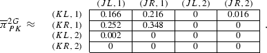
Essentially, since the entry at ((KL, 1), (JR, 2)) is positive, this indicates that the goalkeepers jumped right a little more than optimal, and since the entry ((KL, 2), (JR, 1)) is (barely) positive, this indicates that the kickers kicked left very slightly more than optimal. The remaining entries with (KL, 1), (KR, 1), (JL, 1), and (JR, 1) are all consistent with rationality.
The games and frequencies of play are taken from Goeree and Holt (2001).
We are grateful to Rahul Bhui and Peter Bossaerts for kindly providing us the data for this game.
These are taken from Costa-Gomes et al. (2001). We are grateful to Miguel Costa–Gomes for kindly providing us the data for these experiments.
Kneeland (2015) estimates for an interesting class of “ring games” the degrees to which agents are rational, hold beliefs of opponents being rational, and consistency of beliefs, and deduces that deviations from “equilibrium behavior” are largely due to inconsistency of beliefs.
To see this, notice that the computation of the largest \(\overline{p}\) consistent with payoff maximization and no further constraint must yield a no smaller \(\overline{p}\) than the same computation with the additional constraint of the common prior assumption.
To see that in a (1, 0)-rational belief system the total mass of states where agents are nonrational is unrestricted, take the game in Example 1 and consider the belief system B, where \(\Omega =A\), \(\alpha _{i}(a_{-i};a_{i})=a_{i}\), for any player i and any \(\left( a_{-i};a_{i}\right) \in A\), and where \(\mu \in \Delta (A)\) is given by \(\mu _{TL}=\mu _{TR}=\mu _{BL}=0\) and \(\mu _{BR}=1\). It can be checked that it is (1, 0)-rational and clearly \(\mu [R]=0\). At the same time, in a (p, q)-rational belief system it is always the case that, for any player i and any state \(\omega \), \(\mu (\omega )\left[ R_{-i}\right] \ge q\), hence
$$\begin{aligned} \mu [R_{-i} \cap \Pi _{i}\left( \omega \right) ] \ge q\cdot \mu [\Pi _{i}\left( \omega \right) ]\Longrightarrow \sum _{\Pi _{i}\left( \omega \right) \in \Pi _{i}} \mu [R_{-i} \cap \Pi _{i}\left( \omega \right) ]=q\cdot \sum _{\Pi _{i}\left( \omega \right) \in \Pi _{i}} \mu [\Pi _{i}\left( \omega \right) ]\Longrightarrow \mu [R_{-i}] \ge q \end{aligned}$$which besides confirming the expected convergence to the correlated equilibria as \((p,q) \rightarrow (1,1)\), also shows that positive q’s do put restrictions on the total mass of states where agents are rational \(\mu [R]\).
In order to see it in detail, given game G and probability p we say that a family of distributions \(\left( \pi _{i}\right) _{i\in I}\in \left( \Delta \left( A\right) \right) ^{I}\) is a p-subjectively rational outcome of G (p-SRO(G)) if there exists some belief system B that satisfies MB\(^{p}\)R, does not satisfy the common prior assumption and induces subjective outcomes \((\pi _{i})_{i\in I}\). As shown in the Appendix, it is easy to see that, for any \(p \in [0,1]\), the whole space is obtained, namely:
$$\begin{aligned} p- SRO\left( G\right) =\left( \Delta \left( A\right) \right) ^{I}. \end{aligned}$$In particular, a player who is certain that all the other agents are rational may still select a nonrational action, and thus, any pure strategy profile in A is consistent with MB\(^{p}\)R, even when \(p=1\).
Recall that the result of part (i) of Lemma 1 also holds with noncommon priors.
We abbreviate, \(\mu \left[ \prod _{j\ne i}(A_{j}\times \{k\})\cap \Pi _{i}(\omega )\right] =\mu \left[ \left( T\times \prod _{j\ne i}(A_{j}\times \{k\})\times A_{i}'\times \Theta \right) \cap \Pi _{i}(\omega )\right] \), with some abuse of notation.
This follows from \(p^n \ge p^{n-1}\), and because \(\pi \in p\)-RO(G) with \(p \ge p^{n-1}\) implies \(\pi \left[ \left( A^{n-1}\right) ^c \right] \le 1-p\).

References
Aliprantis CD, Border KC (2006) Infinite dimensional analysis: a Hitchhiker’s guide, 3rd edn. Springer, Berlin
Aumann RJ (1974) Subjectivity and correlation in randomized strategies. J Math Econ 1:67–96
Aumann RJ (1987) Correlated equilibria as an expression of Bayesian rationality. Econometrica 55(1):1–18
Aumann RJ (1992) Irrationality in game theory. In: Dasgupta P, Gale D, Hart O, Maskin E (eds) Economic analysis of markets and games: essays in honor of Frank Hahn. MIT Press, Cambridge
Aumann RJ, Dreze JH (2008) Rational expectations in games. Am Econ Rev 98:72–86
Battigalli P, Di Tillio A, Grillo E, Penta A (2011) Interactive epistemology and solution concepts for games with asymmetric information. BE J Theor Econ 11, Article 6
Bergemann D, Morris S (2015) Bayes correlated equilibrium and the comparison of information structures in games. forthcoming Theoretical Economics
Bernheim BD (1984) Rationalizable strategic behaviour. Econometrica 52:1007–1028
Börgers T (1994) Weak dominance and approximate common knowledge. J Econ Theor 64:265–276
Brandenburger A, Dekel E (1987) Rationalizability and correlated equilibria. Econometrica 55:1391–1402
Camerer CF (2003) Behavioral game theory: experiments in strategic interaction. Princeton University Press, New York
Camerer CF, Ho T-H (2015) Behavioral game theory, experiments and modeling. In: Young HP, Zamir S (eds) Handbook of game theory, vol 4. North-Holland, Elsevier, Amsterdam
Camerer CF, Loewenstein G, Rabin M (2011) Advances in behavioral economics. Princeton University Press, Princeton
Chiappori PA, Levitt SD, Groseclose T (2002) Testing mixed-strategy equilibria when players are heterogeneous: the case of penalty kicks in soccer. Am Econ Rev 92:1138–1151
Conlisk J (1996) Why bounded rationality? J Econ lit 34:669–700
Costa-Gomes M, Crawford VP, Broseta B (2001) Cognition and behavior in normal-form games: an experimental study. Econometrica 69:1193–1235
Crawford VP (2013) Boundedly rational versus optimization-based models of strategic thinking and learning in games. J Econ Lit 51:512–527
Dekel E, Fudenberg D, Morris S (2007) Interim correlated rationalizability. Theor Econ 2:15–40
Forges F (1993) Five legitimate definitions of correlated equilibrium in games with incomplete information. Theor Decis 35:277–310
Forges F (2006) Correlated equilibrium in games with incomplete information revisited. Theor Decis 61:329–344
Germano F, Weinstein J, Zuazo-Garin P (2016) Uncertain rationality, depth of reasoning and robustness in games with incomplete information. Mimeo
Goeree JK, Holt CA (2001) Ten little treasures of game theory and ten intuitive contradictions. Am Econ Rev 91:1402–1422
Harstad RM, Selten R (2013) Bounded-rationality models: tasks to become intellectually competitive. J Econ Lit 51:496–511
Hart S (2005) Adaptive heuristics. Econometrica 73:1401–1430
Hart S, Mansour Y (2010) How long to equilibrium? The communication complexity of uncoupled equilibrium procedures. Games Econ Behav 69:107–126
Hu T-W (2007) On p-rationalizability and approximate common certainty of rationality. J Econ Theor 136:379–391
Kajii A, Morris S (1997) Refinements and higher order beliefs: a unified survey. Mimeo
Kajii Atsushi, Morris Stephen (1997b) The Robustness of Equilibria to Incomplete Information Games. Econometrica 65:1283–1309
Kneeland T (2015) Identifying higher-order rationality. Econometrica 83:2065–2079
Lehrer E, Rosenberg D, Shmaya E (2010) Signaling and mediation in games with common interest. Games Econ Behav 68:670–682
Lehrer E, Rosenberg D, Shmaya E (2013) Garbling of signals and outcome equivalence. Games Econ Behav 81:179–191
Mallard G (2011) Modeling cognitively bounded rationality: an evaluative taxonomy. J Econ Surveys 26:674–704
Martin Christopher F, Bhui R, Bossaerts P, Matsuzawa T, Camerer C (2014) Chimpanzee choice rates in competitive games match equilibrium game theory predictions. Sci Rep 4:5182.1–6
McKelvey RD, Palfrey TR (1995) Quantal Response equilibria for normal form games. Games Econ Behav 10:6–38
Monderer D, Samet D (1989) Approximating common knowledge with common beliefs. Games Econ Behav 1:179–190
Palacios-Huerta I (2003) Professionals play minimax. Rev Econ Stud 70:395–415
Palacios-Huerta I, Volij O (2008) Experiencia docet: professionals play minimax in laboratory experiments. Econometrica 76:71–115
Pearce DG (1984) Rationalizable strategic behaviour and the problem of perfection. Econometrica 52:1029–1050
Rubinstein A (1998) Modelling bounded rationality. MIT Press, Cambridge
Stahl DO II, Wilson PW (1994) Experimental evidence on players’ models of other players. J Econ Behav Org 25:309–327
Stahl DO II, Wilson PW (1995) On players’ models of other players: theory and experimental evidence. Games Econ Behav 10:218–254
Tan Tommy Chin-Chiu, da Costa Werlang Ribeiro Sérgio (1988) The Bayesian foundation of solution concepts of games. J Econ Theor 45:370–391
Wright JR, Leyton-Brown K (2014) Level-0 meta-models for predicting human behavior in games. In: Proceedings of the 15th Conference on Economics and Computation (EC’14)
Author information
Authors and Affiliations
Corresponding author
Additional information
Earlier versions of this paper circulated under the title “Approximate Knowledge of Rationality and Correlated Equilibria.” We are indebted to Bob Aumann, Eddie Dekel, Sergiu Hart, and Dov Samet, for valuable comments and conversations. We also thank an anonymous referee and the editor, Bernhard von Stengel, as well as audiences in Barcelona, Bilbao, Budapest, Chicago, Istanbul, Jerusalem, Marseille, Paris, and York for insightful comments. Germano acknowledges financial support from the Spanish Ministry of Economy and Competitiveness (Grant ECO2014-59225-P), as well as from the Barcelona GSE Research Network and the Generalitat de Catalunya. Zuazo-Garin acknowledges financial support from the Spanish Ministry of Science and Technology (Grant ECO2009-11213), from the Spanish Ministry of Economy and Competitiveness (Grant ECO2012-31326) and from the Basque Government (Grants IT568-13 and POS-2015-1-0022), as well as inestimable help from professors Elena Iñarra and Annick Laruelle. Both authors thank the Center for the Study of Rationality at the Hebrew University of Jerusalem for their generous hospitality; Germano also thanks AMSE-IMéRA at Université Aix-Marseille and Zuazo-Garin thanks the Game Theory Group at Tel Aviv University and the CMS-EMS at Northwestern University for their generous hospitality. All errors are our own.
Appendices
APPENDIX
1.1 A Proof of Lemma 1
-
(i)
The left implication is obvious, so let’s focus on the right one. By definition, \(CB^{p}\left( R\right) \subseteq \bigcap _{i\in I}B_{i}^{p}\left( R\right) \), and therefore, for any \(i\in I\), \(CB^{p}\left( R\right) \subseteq B_{i}^{p}\left( R_{i}\right) \). Then, since \(p>0\), and \(\omega \in B_{i}^{p}\left( R_{i}\right) \), we have that \(R_{i}\cap \Pi _{i}\left( \omega \right) \ne \emptyset \), and therefore, that \(\Pi _{i}\left( \omega \right) \subseteq R_{i}\) and, in particular, \(\omega \in R_{i}\). Thus, \(B_{i}^{p}\left( R_{i}\right) \subseteq R_{i}\).
-
(ii)
It is immediate that \(CB^{1}\left( R\right) =\Omega \) if and only of \(\bigcap _{i\in I}B_{i}^{1}\left( R\right) =\Omega \), so it suffices to prove that \(\bigcap _{i\in I}B_{i}^{1}\left( R\right) =\Omega \) if and only if \(\bigcap _{i\in I}B_{i}^{1}\left( R_{-i}\right) =\Omega \). The right implication is immediate. For the proof of the left one, from part (i) of the lemma, it is enough to check that if \(\bigcap _{i\in I}B_{i}^{1}\left( R_{-i}\right) =\Omega \) then \(R=\Omega \). But this is immediate: take \(i,j\in I\), \(i\ne j\), then \(B_{j}^{p_{j}}\left( R_{-j}\right) \subseteq B_{j}^{p_{j}}\left( R_{i}\right) \), and therefore, \(B_{j}^{p_{j}}\left( R_{i}\right) =\Omega \). Hence \(\mu \left( R_{i}\right) = \sum _{\omega \in \Omega } \mu \left( R_{i}\cap \Pi _{j}\left( \omega \right) \right) = \sum _{\omega \in \Omega } \mu \left( \Pi _{j}\left( \omega \right) \right) =1\). Since \(\mu \) has full support on \(\Omega \), the latter implies that \(R_{i}=\Omega \). As the proof applies for any \(i\in I\), we obtain that \(R=\Omega \).
-
(iii)
If \(\bigcap _{i\in I}B_{i}^{p}\left( R_{-i}\right) =\Omega \), then \(R=\bigcap _{i\in I}\left( B_{i}^{p}\left( R_{-i}\right) \cap R_{i} \right) =\bigcap _{i\in I}B_{i}^{p}\left( R\right) \). Thus, R is p-evident belief and therefore, \(R\subseteq CB^{p}(R)\). Now, since \(\bigcap _{i\in I}B_{i}^{p}\left( R_{-i}\right) =\Omega \), we have both that \(\mu \left[ R_{-i}\right] \ge p\) and \(\mu \left[ R_{-i}\cap R_{i}\right] \ge p\cdot \mu \left[ R_{i}\right] \). The former implies that that \(\mu [R_{j}]\ge p\) for any \(j\ne i\); and thus, the same argument and some reindexing imply that \(\mu [R_{i}]\ge p\). The fact that for any \(j\ne i\), \(\mu \left[ R\right] =\mu \left[ R_{-i}|R_{i}\right] \cdot \mu \left[ R_{i}\right] \ge p\cdot \mu \left[ R_{i}\right] \ge p^{2}\) completes the proof.
B Proofs of the characterization results
In this section we first prove a technical lemma. Then we prove Theorem 4, and then Theorem 1 as a special case of Theorem 4. The technical lemma is the following:
Lemma 2
Let \(\left( G,S\right) \) be a Bayesian game, p a probability, \(n\in \{2,3\}\), and \(\pi ^{*}\in \left( A_{(k)}, p\right) \)-\(BCE\left( nG,S\right) \) for some \(k\le n\). For game nG, let belief system \(B=\left\langle \Omega ,\left( \Pi _{i}\right) _{i\in I},\mu ,\kappa ,\left( \alpha _{i}\right) _{i\in I},\left( \tau _{i}\right) _{i\in I}\right\rangle \) be given by: (i) \(\Omega =\left\{ \left( t,a,\nu ,\theta \right) \in T\times A'\times \Theta \right. \left. \left| \pi ^{*}\left[ \left( a,\nu ,\theta \right) \right] >0\right. \right\} \), and for any \(\left( t,a,\nu ,\theta \right) \in \Omega \), (ii) \(\mu \left[ (t,a,\nu ,\theta )\right] =\pi ^{*}\left[ \left( t,a,\nu ,\theta \right) \right] \), (iii) \(\kappa \left( t,a,\nu ,\theta \right) =\theta \), and for any \(i\in I\), (iv) we have cells \(\Pi _{i}\left( t,a,\nu ,\theta \right) =T_{-i}\times A'_{-i}\times \Theta \times \left\{ (t_{i},a_{i},\nu _{i})\right\} \), (v) \(\alpha _{i}\left( t,a,\nu ,\theta \right) =a_{i}\), and (vi) \(\tau _{i}\left( t,a,\nu ,\theta \right) =t_{i}\). Then, B is a belief system for (G, S) satisfying consistency, MB\(^{p}\)R and the common prior assumption, and induces \(\pi ^{*}\) in \(T\times A'\times \Theta \).
Proof
It is immediate that \(\alpha _{i}\) and \(\tau _{i}\) are measurable w.r.t. \(\Pi _{i}\) for any \(i\in I\). Take \(\left( t,\theta \right) \in T\times \Theta \); then, we have \(\mu \left[ \tau =t,\kappa =\theta \right] =\pi ^{*}\left[ \left( t,\theta \right) \right] =\psi \left[ \theta \right] \cdot \sigma \left[ t|\theta \right] \), and therefore, B satisfies consistency. Now, note first the fact that for any \(\omega =(t,a,\nu ,\theta )\in \Omega \) and any \(a'_{i}\in A_{i}\) it holds that,
together with the incentive constraints, implies that for any \(i\in I\) we have that \(T\times A_{-i}'\times (A_{i}\times \{k\})\times \Theta \subseteq R_{i}\), and therefore,Footnote 24 that \(\mu \left[ \prod _{j\ne i}(A_{j}\times \{k\})\cap \Pi _{i}(\omega )\right] \le \mu \left[ R_{-i}\cap \Pi _{i}(\omega )\right] \) for any \(i\in I\) and any \(\omega \in \Omega \). Then, take \(i\in I\) and \(\omega =(t,a,\nu ,\theta )\in \Omega \) and note that:
In consequence, due to the p-belief constraints, we have \(\mu \left[ R_{-i}\cap \Pi _{i}(\omega )\right] \ge p\cdot \mu \left[ \Pi _{i}(\omega )\right] \), and therefore, that B satisfies MB\(^{p}\)R. \(\square \)
1.1 B.1 Proof of Theorem 4
For the right inclusion, pick \(\pi \in p\)-\(RBO\left( G,S\right) \) and B, a belief model that induces \(\pi \). Take distribution \(\pi ^{*}\in \Delta \left( T\times A'\times \Theta \right) \) given by,
for any \((t,a,\nu ,\theta )\in T\times A'\times \Theta \). Then, \(\pi ^{*}\in \Delta \left( T\times A'\times \Theta \right) \). The consistency constraint is satisfied, since,
for any \(\left( t,\theta \right) \in T\times \Theta \). Now, note that for any \(i\in I\), any \(a_{i},a'_{i}\in A_{i}\), any \(t_{i}\in T_{i}\) and any \(\nu _{i}\in N\) we have that,
In addition, note that for any \((t_{i},a_{i},\nu _{i})\in T_{i}\times A'_{i}\),
Thus, both the incentive constraints and the p-belief constraints are satisfied. For the left inclusion, just apply Lemma 2 to \(A_{i}'=A_{i}\times \{1,2\}\) and \(k=1\).
1.2 B.2 Proof of Theorem 1
This theorem can be seen as a corollary of Theorem 4. To see this, note that if G is a game with complete information, we can define Bayesian game \(\left( G',S\right) \), where we have (i) \(G'=\left\langle I,\Theta ,\psi ,\left( A_{i}\right) _{i\in I},\left( u'_{i}\right) _{i\in I}\right\rangle \), with \(\Theta =\left\{ \theta \right\} \), \(\psi =1_{\left\{ \theta \right\} }\) and \(u'_{i}(a,\theta )=u_{i}(a)\) for any \(a\in A\) and \(i\in I\), and (ii) \(S=\left\langle \left( T_{i}\right) _{i\in I},\sigma \right\rangle \) with \(T_{i}=\left\{ t_{i}\right\} \) for any \(i\in I\) and \(\sigma (t|\theta )=1\). It is immediate that, for any \(X=\prod _{i\in I}X_{i}\subseteq A\) and any \(p\in [0,1]\), we have that \(\left( X,p\right) - CE\left( G\right) =\left( X,p\right) - BCE\left( G',S\right) \). But note also that if we take some list \(B'=\left\langle \Omega ,\left( \Pi _{i}\right) _{i\in I},\left( \alpha _{i}\right) _{i\in I},\left( \tau _{i}\right) _{i\in I},\mu \right\rangle \), which is a candidate to be a belief system for \(G'\), for any \(i\in I\), forcefully \(\tau _{i}=1_{\left\{ t_{i}\right\} }\); and therefore, \(B'\) is a belief system for \(G'\) if and only if \(B=\left\langle \Omega ,\left( \Pi _{i}\right) _{i\in I},\left( \alpha _{i}\right) _{i\in I},\mu \right\rangle \) is a belief system for G. Thus, it is immediate that, for any \(p\in [0,1]\), we have \(p- RO\left( G\right) = p- RBO\left( G',S\right) \). So, let G be a game, and \(p\in [0,1]\). Then, we just checked above that both \(p- RO\left( G\right) =p- RBO\left( G',S\right) \) and \(\left( A_{(1)},p\right) - CE\left( 2G\right) =\left( A_{(1)},p\right) - BCE\left( 2G',S\right) \), hold, so from Theorem 4 we conclude that \(p- RO\left( G\right) = \left( A_{(1)},p\right) - CE\left( 2G\right) \).
1.3 B.3 Proof of Theorem 3
We prove the first statement; the next one concerning the p-rational expectations of rational types then follows directly. We suppose we are taking some player i’s expectation. For right inclusion, take p-rational belief system \(B=\left\langle \Omega ,\left( \Pi _{i}\right) _{i\in I},\left( \alpha _{i}\right) _{i\in I},\mu \right\rangle \) and \(\omega \in \Omega \). We define:
for any \((a,\nu )\in A'\), where \(W_{i}=R_{i}{\setminus }\Pi _{i}\left( \omega \right) \) if \(\nu _{i}=0\), \(W_{i}=\lnot \left( R_{i}{\setminus }\Pi _{i}\left( \omega \right) \right) \) if \(\nu _{i}=1\), and \(W_{i}=\Pi _{i}\left( \omega \right) \) if \(\nu _{i}=2\). It is immediate that \(\pi _{i,\omega }^{*}\in \Delta \left( A'\right) \). By an argument similar to the one in the first part of the proof of Theorem 4, reduced to the degenerate case where \(|\Theta |=1\), we can conclude that \(\pi _{i,\omega }\) is a \(\left( A_{(1)},p\right) \)-correlated equilibrium of G; moreover, it is immediate that player i’s expectation conditional on playing \(\left( \alpha _{i}\left( \omega \right) ,3\right) \) induced by \(\pi _{i,\omega }\) is exactly \(\mathbb {E}(\omega )\left[ u_{i}\left( \alpha _{-i},\alpha _{i}\left( \omega \right) \right) \right] \). For the left inclusion, take Lemma 2 for the case \(A'_{i}=A_{i}\times \{1,2,3\}\), \(k=1\), and \(|\Theta |=1\).
C Proof of Theorem 2
Nonemptiness follows from the fact that correlated equilibria always exist for any finite game G and constitute p-rational outcomes for any \(p\in [0,1]\). Given that the set of p-rational outcomes is a projection of the (X, p)-correlated equilibria of 2G, with \(X=A_{(k)}\) a copy of the action space of the original game G, the remaining properties follow once they have been shown for the (X, p)-correlated equilibria of 2G. This is what we do next. For the given game G, define the (X, p)-correlated equilibrium correspondence, where \(X=A _{(k)}\) with \(k \in \{0, 1\}\), is fixed:

Clearly \(\rho \) is convex- and compact-valued; it remains to be shown that it is also continuous. We do this by showing that it is upper- and lower-hemicontinuous (respectively, uhc and lhc) as a correspondence of p.

Since 2A is finite, \(\Delta (2A)\) is compact, and hence upper-hemicontinuity is equivalent to showing that \(\rho \) has a closed graph. But this is immediate from inspection of the inequalities defining the sets \((X, p)- CE\left( 2G\right) \). In particular, all the inequalities are all weak inequalities, linear in p. Moreover, the domain [0, 1] is compact.

Denote by \(\Gamma _{\rho } \subset [0,1]\times \Delta (2A)\) the graph of the correspondence \(\rho \). Fix \((p, \hat{\pi }) \in \Gamma _{\rho }\) and let \(\left( p^n\right) _n \subset [0,1]\) be a sequence converging to p. We need to show that there exists a sequence \(\left( (\hat{\pi })^n\right) _n\) converging to \(\hat{\pi }\) such that \((\hat{\pi })^n \in \rho (p^n)\) for sufficiently large n. Take the point \((p, \hat{\pi })\). Clearly this satisfies all inequalities defining \(\rho (p)\), in particular also the p-rationality constraints. Consider the following sequence \(\left( p^n, \hat{\pi }\right) _n \subset [0,1] \times \Delta (2A)\). If for sufficiently large n the elements are contained in \(\Gamma _{\rho }\) we are done. So consider the case where they are not. Consider the family of projections \(\Pi _{\rho }: [0,1] \times \Delta (2A) \longrightarrow [0,1] \times \Delta (2A)\) that map, for fixed \(\bar{p} \in [0,1]\), any element \((\bar{p}, \bar{\pi }) \in [0,1] \times \Delta (2A)\) to the point in the set \(\{ \bar{p} \} \times \rho ( \bar{p} )\) that is closest to \((\bar{p}, \bar{\pi })\). Since the sets \(\rho ( \cdot )\) are always nonempty, convex, compact polyhedra, we have that \(\Pi _{\rho } \left( p^n, \hat{\pi } \right) \) is uniquely defined and moreover, \(\Pi _{\rho } \left( p^n, \hat{\pi } \right) \in \Gamma _{\rho }\) for any point in the sequence \(\left( p^n, \hat{\pi } \right) _n\). It remains to be shown that the sequence \(\left( \Pi _{\rho } \left( p^n, \hat{\pi } \right) \right) _n\) converges to the point \((p, \hat{\pi })\). Apart from the p-belief constraints all other constraints defining \(\rho (p)\) are independent of p. Hence, if \((p, \hat{\pi })\) satisfies those constraints, then so must any other point in the sequence \(\left( p^n, \hat{\pi }\right) _n\). Therefore the only constraints that can be violated by elements of the sequence \(\left( p^n, \hat{\pi }\right) _n\) are the p-belief constraints. Consequently, any point in the sequence \(\left( \Pi _{\rho } \left( p^n, \hat{\pi } \right) \right) _n\) lies on the boundary of the polyhedra defined by the p-belief constraints. As mentioned, these constraints are linear in p, and since they also define nonempty, convex, compact polyhedra, the sequence \(\left( \Pi _{\rho } \left( p^n, \hat{\pi } \right) \right) _n\) indeed converges to \((p, \hat{\pi })\). This shows the continuity of \(\rho \) and hence also of p-RO(G) in p.
Finally, the claims that, for \(p=0\), we have 0-\(RO(G)=\Delta (A)\), and for \(p=1\), we have 1-\(RO(G)=CE(G)\), are immediate. To see that for any \(p \in [0,1)\), we have dim[p-\(RO(G)]=\) dim\([\Delta (A)]\), notice that the (X, p)-correlated equilibria with \(X=A^1\) and \(p<1\) entail distributions that put strictly positive weight on all strategies in \(A^2\) as well as all convex combinations of such distributions. Projecting onto the original space \(\Delta (A)\) implies distributions with strictly positive weights on all strategies in A as well as all possible convex combinations. This concludes the proof.
D Proof of Proposition 1
Fix G and let \(A^n=\Pi _{i \in I} A_i^n\) denote the space of all pure strategy profiles that survive n rounds of iterated elimination of strictly dominated strategies in G, and similarly for the individual sets \(A_i^n\). Let \(G^n\) denote the subgame of G with strategies restricted to \(A^n\). Because G is finite, the limit sets \(A_i^{\infty }, A^{\infty }\), and \(G^{\infty }\) are well defined (and are obtained after finitely many iterations). Also, for any subset \(Y \subset A\), let \(Y^c=A{\setminus } Y\) denote the complement of Y in A. For any given \(p\in \left[ 0,1\right] \), take \(p'\ge p\). We show that for p sufficiently close to 1, behavior is supported with high probability in \(A^{\infty }\). Specifically, we construct a \(\bar{p}<1\) such that for any \(p \in [\bar{p}, 1]\), if \(\pi \in p\)-RO(G), then \(\pi \left[ \left( A^{\infty }\right) ^c \right] \le 1-p\). Consider the game \(G^0=G\) and pick some \(p^1<1\). It immediately follows from p-rationality that for \(p\in [p^1,1]\), if \(\pi \in p\)-RO(G), then we have \(\pi \left[ \left( A^1\right) ^c \right] \le 1-p\). Suppose now that the above statement is true for \(n-1\), namely there exists \(p^{n-1}<1\) such that for \(p \in [p^{n-1},1]\), if \(\pi \in p\)-RO(G), then we have \(\pi \left[ \left( A^{n-1}\right) ^c \right] \le 1-p\). We show that the statement also holds for n. Fix game \(G^{n-1}\). It follows from finiteness of G and continuity of the payoffs that there exists \(p^n \in [p^{n-1}, 1)\) such a strategy in \(A^{n-1}{\setminus } A^n\) that is strictly dominated in \(G^{n-1}\) (by some strategy in \(G^{n-1}\) and hence in G) is also strictly dominated in G (by the same strategy) given a p-rational belief system with \(p \ge p^n\).Footnote 25 This implies that for any \(p \in [p^n, 1]\) and any \(\pi \in p\)-RO(G), we also have \(\pi \left[ \left( A^n\right) ^c\right] \le 1-p\). Finiteness of the game implies that the process ends after finitely many steps implying that indeed there exists \(p^{\infty } <1\) such that for \(p \in [p^{\infty }, 1]\) and any \(\pi \in p\)-RO(G), we have \(\pi \left[ \left( A^{\infty }\right) ^c \right] \le 1-p\). Taking \(\bar{p}=p^{\infty }\) proves the claim.
E Proof of Proposition 2
To see the if part, take \(\pi \in \Delta (A)\) a p-rational outcome of G. By Theorem 1, there exists an \((A_{(1)}, p)\)-correlated equilibrium \(\hat{\pi } \in \Delta (A')\) of the doubled game 2G. Define \(P \equiv \hat{\pi }\) and set
for all \(t_{i} \in T_{i}\). Then, by definition of the type spaces \(T_{i}=T_{i}^{s} \cup T_{i}^{c}\), we have:
-
\(P[ T^{s}_{-i} \, | \, t_{i}] \ge p\), for any \(t_{i} \in T_{i}\);
-
\(\alpha _{i} (t_{i})[a_{i}]= 1\) if \(t_{i} \in T^{c}_{i}\) and \(t_{i}= a_{i}\)
-
\(a_{i} \in \) argmax\(_{a_{i}' \in A_{i}} \sum _{t_{-i} \in T_{-i}}P[t_{-i} \, | \, t_{i}]\cdot \sum _{a_{-i} \in A_{-i}}\alpha _{-i} (t_{-i})[a_{-i}]\cdot u_{i}(a_{-i};a_{i}')\), where \(\alpha _{-i}(t_{-i})[a_{-i}]=\prod _{j\ne i}\alpha _{j}(t_{j})[a_{j}]\).
Let \(\mu [a]=\sum _{t \in T}P(t)\cdot \alpha (t)[a]\), where \(\alpha (t)[a]=\prod _{i\in I}\alpha _{i}(t_{i})[a_{i}]\); then, again by construction, and using Theorem 1, we have \(\mu = \pi \).
To see the only if part, take \(\mu \in \Delta (A)\) an EAD of (G, P) where P satisfies \(P[ T^{s}_{-i} \, | \, t_{i}] \ge p\), for any \(t_{i} \in T_{i}\), and for some equilibrium profile \(\alpha \) satisfying conditions (i) and (ii). By definition, together with P, \(\alpha \) can be seen as inducing a probability distribution on the outcomes of the doubled game \(\hat{\mu } \in \Delta (2A)\), where types in \(T_{i}^{s}\) and corresponding strategies chosen are associated to \(A_{(2)}\) and types in \(T_{i}^{c}\) are associated to strategies in \(A_{(2)}\). As a consequence of (i) and (ii) and the definition of P, \(\hat{\mu }\) will also satisfy the incentive constraints and the p-belief constraints for 2G. By Theorem 1, computing the EAD \(\mu \) of \(\hat{\mu }\) gives us, a p-rational outcome of G.
F Proof of result in Remark 2
Adapting the original definition by Aumann (1974), Aumann (1987), for any \(X=\prod _{i\in I}X_{i}\subseteq A\), we say that the family \(\left( \pi _{i}\right) _{i\in I}\subseteq \left( \Delta \left( A\right) \right) ^{I}\) is a \(\left( X,p\right) \)-subjective correlated equilibrium of G, if, for any \(i\in I\) the following are satisfied:
-
Incentive constraints For any \(a_{i}\in X_{i}\), \(a_{i}\in \text {argmax}_{a'_{i}\in A_{i}}\sum _{a_{-i}\in A_{-i}}\pi _{i}[\left( a_{-i};a_{i}\right) ]\cdot u_{i}\left( a_{-i};a'_{i}\right) \).
-
p-Belief constraints For any \(a_{i}\in A_{i}\), \(\pi _{i}\left[ X_{-i}\times \{a_{i}\}\right] \ge p\cdot \pi _{i}\left[ A_{-i}\times \{a_{i}\}\right] \).
We denote the set of \(\left( X,p\right) \)-subjective correlated equilibria of game G by \(\left( X,p\right) - SCE\left( G\right) \). Given \(n\in \{2,3\}\) and nG, we have a map \(\mathbf marg _{A^{I}}:\left( \Delta \left( A'\right) \right) ^{I}\rightarrow \left( \Delta \left( A\right) \right) ^{I}\), where for any \(\left( \hat{\pi _{i}}\right) _{i\in I}\in \left( \Delta \left( A'\right) \right) ^{I}\), we have that \(\mathbf{marg }_{A^{I}}\left( \left( \hat{\pi _{i}}\right) _{i\in I}\right) =\left( \text {marg}_{A}\left( \hat{\pi _{i}}\right) \right) _{i\in I}\). Then, the proof of the identity,
where \(X=\prod _{i\in I}\left( A_{i}\times \left\{ 1\right\} \right) \), is the same as the one for Theorem 1 after slight modifications (just add sub-indices where needed). To see that the above marginals constitute the whole space, take \(\left( a^{i}\right) _{i\in I}\subseteq A\), and for any \(i\in I\), \(\pi _{i}=1_{\left\{ a^{i}\right\} }\). Fix \(k\in \left\{ 1,2\right\} \), and define, for any \(i\in I\), \(\hat{\pi }_{i}=1_{\{((a_{j}^{i},k)_{j\ne i};(a_{i}^{i},2-k))\}}\). It is immediate that \(\mathbf{marg }_{A^{I}}\left( \left( \hat{\pi }_{i}\right) _{i\in I}\right) =\left( \pi _{i}\right) _{i\in I}\). Now, take \(i\in I\), then the incentive constraints are trivially satisfied, since \(\hat{\pi }_{i}[A_{i}\times \left\{ 1\right\} ]=0\). Moreover, the p-belief constraint is also satisfied, because, regardless of i’s action, the sums are on both sides 0 or 1. We conclude that, again for \(X=\prod _{i\in I}\left( A_{i}\times \left\{ 1\right\} \right) \), we have \(\left( 1_{\{a^{i}\}}\right) _{i\in I}\in \mathbf{marg }_{A^{I}}((X ,p)- SCE(2G))\) for any \((a^{i})_{i\in I}\subseteq A\); thus, by convexity, \(\mathbf{marg }_{A^{I}}((X ,p)- SCE(2G))=((\Delta \left( A\right) )^{I}\).
Rights and permissions
About this article

Cite this article
Germano, F., Zuazo-Garin, P. Bounded rationality and correlated equilibria. Int J Game Theory 46, 595–629 (2017). https://doi.org/10.1007/s00182-016-0547-5
Accepted:
Published:
Issue Date:
DOI: https://doi.org/10.1007/s00182-016-0547-5
Keywords
- Strategic interaction
- Correlated equilibrium
- Robustness to bounded rationality
- Approximate knowledge
- Incomplete information
- Measure of rationality
- Experiments