A real-time and precise ellipse detector via edge screening and aggregation

Abstract

A fast and precise method for ellipse detection is proposed in this paper. The method aims at clearly removing the lines and curves which are not ellipse edges to improve the ellipse fitting. In arc extraction, the arcs are divided into four categories according to the gradient, and the size constraint is exploited to remove the interference lines. Then, the arc relative position constraints and the tangent lines constraint are employed to exactly group the arcs that belong to the same ellipse into a set. Finally, a post-processing approach is developed to remove the invalid ellipses. Due to the effective removal of the interference edges and the designed geometric multi-constraint, the computational costs of arc grouping and parameter estimation are dramatically reduced, and the fitting results are finely agreeable to the actual ellipse contours. The performance is evaluated with 3600 synthetic images and 1517 real images, and the experimental results demonstrate that the proposed method runs much faster than the current speed leading methods with the comparable or higher F-measure.

1 Introduction

Circular structure is one of the fundamental structures in industrial parts and tools. Since the circular structure often appears as an ellipse in the image, ellipse detection has become an important task in the field of machine vision applications. For instance, ellipse detection has been widely used in cameral calibration [1, 2], relative pose and position measurement [3, 4], 3D reconstruction [5] and object segmentation [6]. Therefore, it has become more and more important to detect ellipses precisely and efficiently for some visual measurement or recognition tasks, especially in the complex environments.

Generally, the ellipse detection methods can be divided into four categories, including the Hough transform-based methods, the least square fitting-based methods, the edge following-based methods and the line segment-based methods.

Hough transform (HT) was firstly introduced in [7] to detect lines and curves in images and then was further developed for ellipse detection. In the Hough transform-based ellipse detection, the image is first transformed into the parametric space and then, the ellipse parameters are estimated by finding the peaks in the parametric space. Analogously, the Radon transform [8] is used to transform the image into the parameter space and obtain the prominent features in the projection direction. To improve the flexibility, HT was generalized to detect the arbitrary non-analytic shapes by Ballard [9]. However, due to the high-dimensional parameter space and the long voting procedure on the edge pixel plenty, low computational efficiency and huge memory demand occurred in this kind of methods, which limits their application. To speed up the HT-based ellipse detection, the randomized Hough transform (RHT) [10], the probabilistic Hough transform (PHT) [11, 12] and the iterative randomized Hough transform (IRHT) [13] were proposed. RHT and PHT use the sampled pixels to vote on the parameters of ellipses for improving the computational efficiency. IRHT further accelerates the RHT by focusing on the region of interest which is determined from the latest estimation of ellipse parameters. Although these methods reduce the number of edge points for estimating ellipse parameters, the running time is still difficult to satisfy many real-time detection applications. Besides, since it is difficult to identify the true peaks in the parametric space, the detection accuracy decreases rapidly with the increasing of the ellipse number in an image [14, 15]. Recently, Chen et al. [16] proposed an edge following-based method to extract the majority of an ellipse. The regions which may contain a missed ellipse are extracted by clustering analysis, and then, a HT-based method is performed to extract the missed ellipse. However, this method requires to predefine the target size and the length of the horizontal view. In addition, it cannot ensure the measurement accuracy, if the ellipses in an image have a big difference in size.

The least square fitting methods are mainly based on the work of Fitzgibbon et al. [17]. The algebraic equation of general conics is used to define an error minimization problem, and the additional numeric constraints are introduced to restrict the solutions of the elliptic curves. The constrained minimization problem is solved by using generalized eigenvalue decomposition. This method provides a least square elliptical fitting solution to any set of edge pixels. Prasad et al. [18] split the mathematical problem of ellipse fitting into two operators, such that the overall algorithm was non-iterative and did not involve constrained optimization. Liang et al. [19] introduced the maximum correntropy criterion into the constrained least square ellipse fitting method and applied the half-quadratic optimization algorithm to solve the nonlinear and nonconvex problem in an alternate manner. Mulleti and Seelamantula [20] proposed a method based on the finite-rate-of-innovation signal property of the ellipse parametric functions. Lowpass filtering technique was used to estimate the uniform samples for reducing the effect of noise. A modified annihilating filter with linear least square was used to estimate the ellipse parameters. Liu et al. [21, 22] detected the candidate circles based on a measure of top-down least square fitting analysis, where “top-down” means that the sub-chains of a given edge segment were verified from the longer ones to the shorter ones. However, most least square fitting methods focus on how to fit an ellipse from the scattering points; thus, it is unable to recognize outliers caused by noise. If the interference of the non-elliptical arcs and the arcs belonging to different ellipse are removed, the accuracy of the least square fitting-based methods will be greatly improved.

Lately, some researchers have tried edge following techniques to detect ellipse. Prasad et al. [23] used the edge curvature and convexity to determine whether the edge contours can be grouped together and performed two-dimensional Hough transform to get ellipse parameters. Fornaciari et al. [24] selected the candidate arcs according to the relationship of the ellipse chord and its center and estimated the parameters via the decomposed parameter space. Jia et al. [25] improved the Fornaciari’s method by applying line pruning progress before parameters estimation. The algorithm leverages a projective invariant to prune the undesired candidates. Jin et al. [26] added the distance constraint to the arc grouping step of Jia’s method [25] to improve the grouping results. Dong et al. [27] reduced the arc number of each group from three to two. The recall of ellipse detection increases, while the false detection also increases, and the detection becomes slower. These methods are hard to recognize the true ellipse edge, if two arc segments are with the similar position and curvature. Therefore, in some cases, the false edge is left after the clustering progress.

Ellipse and line segment detector (ELSD) [28, 29] is a non-iterative ellipse fitting method. It merges the algebraic distance by the gradient orientation. The polygonal approximation of the curve is obtained through a recursive scheme following the rules of convexity and smoothness. Liu et al. [30] used linear segmentation to extract the straight-line segments from the edge contours and implemented a graph model to segment each line contour into elliptical arcs. The least square algorithm was used to estimate the elliptic parameters.

Both the edge following methods and the line segment methods can detect the edge curves which are similar to the elliptic arcs. However, due to the lack of strong geometry constraints, some non-elliptical shadows and arcs also participate in the fitting. This kind of methods is more concerned with the number of the detected ellipses than the accuracy.

In fact, for the images with complex background, it is a key issue to effectively recognize the edges belonging to the same ellipse for fast ellipse detection.

In this paper, a real-time ellipse detector with high detection accuracy is proposed. As shown in Fig. 1, the overall procedure of the proposed method mainly includes three steps, arc extraction, arc grouping and parameter estimation and post-processing. The specific contributions of the proposed method are summarized as follows.

Fig. 1

The flowchart of the proposed method

• (1) The gradient-based edge classification method is proposed for fast arc extraction. In the proposed method, the edge classification depends on only the edge gradient and is independent of bounding box and convexity; therefore, the computation cost is greatly reduced.

• (2) The specific size constraint is defined to remove the interference edges, such as the edges containing a small number of pixels and the edges containing mostly collinear points.

• (3) A new arc grouping method is proposed to fast group the edges belonging to the same ellipse, which largely improves the grouping efficiency.

• (4) A reliability discriminant indicator is developed for validation. By the definition of two validation index, score and reliability, the false detected ellipses can be clearly removed.

2 Arc extraction

Canny edge detector [31] with automatic thresholding is employed to detect edges. The thresholds of Canny detector are adaptively determined by the cumulative distribution of intensity gradients. The edges are divided into four categories according to the gradient afterward. Then, size constraint is leveraged to remove interference edges.

2.1 Edge classification

Given an edge point $e_{i} = \left( {x_{i} ,y_{i} ,{\text{d}}x_{i} ,{\text{d}}y_{i} } \right)$ obtained by Canny edge detector, where’ $\left( {x_{i} ,y_{i} } \right)$ is the position coordinate and $\left( {{\text{d}}x_{i} ,{\text{d}}y_{i} } \right)$ is the Sobel derivative in X and Y orientations, respectively, the slope at this point is obtained by

$$ \tan \varphi_{i} = - \frac{{{\text{d}}x_{i} }}{{{\text{d}}y_{i} }} $$

(1)

where $\varphi_{i}$ is the angle between the tangent line at this point and the positive direction of the horizontal axis. The pixels are discarded if $\tan \varphi_{i}$ is exactly equal to zero. Define $S_{ + }$ as the set of the edge points with positive, and $S_{ - }$ as the set of the left edge points. An arc is formed by link each edge point with the other points in its eight neighborhoods in the same set.

As shown in Fig. 2, by comparing the values of slope in left ($\tan \varphi_{\text{left}}$) and right ($\tan \varphi_{\text{right}}$) ends, an arc $\alpha$ is classified into one of the four categories according to the following equation.

Fig. 2

Classify the arcs into four categories

$$ \alpha \in \left\{ {\begin{array}{*{20}l} {\alpha^{\text{I}} } \hfill & {{\text{if}}\;an\varphi > 0 \wedge \tan \varphi_{\text{left}} < \tan \varphi_{\text{right}} } \hfill \\ {\alpha^{\text{II}} } \hfill & {{\text{if}}\;\tan \varphi < 0 \wedge \tan \varphi_{\text{left}} < \tan \varphi_{\text{right}} } \hfill \\ {\alpha^{\text{III}} } \hfill & {{\text{if}}\;\tan \varphi > 0 \wedge \tan \varphi_{\text{left}} > \tan \varphi_{\text{right}} } \hfill \\ {\alpha^{\text{IV}} } \hfill & {{\text{if}}\;\tan \varphi < 0 \wedge \tan \varphi_{\text{left}} > \tan \varphi_{\text{right}} } \hfill \\ \end{array} } \right. . $$

(2)

2.2 Size constraint

After classification, some arcs, denoted by $\alpha_{k}$, are not salient enough to characterize an ellipse, such as the arcs containing a small number of pixels and the arcs containing mostly collinear points. These arcs need to be removed since they may cause false detection.

Define ${\text{ORI}}_{k}$ as the oriented minimum area rectangle [32] enclosing all edge points $e_{i} \in \alpha_{k}$. For clarity, the oriented minimum area rectangle is the minimum area rectangle containing the curve. The arcs which meet one of the following conditions will be removed:

• (1) The number of points in the arc is smaller than the defined threshold ($N_{k} < {\text{Th}}_{\text{length}}$).

• (2) The length of the short side (${\text{sh}}_{k}$) of ${\text{ORI}}_{k}$ is smaller than the defined threshold (${\text{sh}}_{k} < {\text{Th}}_{\text{short}}$).

• (3) The ratio (${\text{RA}}_{k}$.) of the long side length and the short side length is larger than the defined threshold (${\text{RA}}_{k} > {\text{Th}}_{\text{ratio}}$).

In this work, the values of ${\text{Th}}_{\text{length}}$ and ${\text{Th}}_{\text{short}}$ are set as 16 and 3, respectively. The value of ${\text{Th}}_{\text{ratio}}$ is determined through experiments. Relying on the Sobel derivatives, the arcs are classified into four categories and the invalid edges are removed.

3 Arc grouping and parameter estimation

After edge classification and invalid edge removal, the arcs belonging to the same ellipse are grouped, and then the parameters of the ellipses are estimated. The relative position constraint and the tangent lines constraint are defined for arc grouping. For each group of arcs, the direct least square fitting is used to estimate ellipse parameters.

3.1 Relative position constraint

The relative position relation is designed to ensure that the four arcs ($\alpha_{i}^{\text{I}} ,\alpha_{j}^{\text{II}} ,\alpha_{k}^{\text{III}} ,\alpha_{m}^{\text{IV}}$) from four categories are possible to form an ellipse. Here, a mark of validity $\gamma$ is defined to determine whether the arcs satisfy the relative position constraint as follows.

$$ \gamma \left( {\alpha_{j}^{\text{I}} ,\alpha_{j}^{\text{II}} ,\alpha_{j}^{\text{III}} ,\alpha_{j}^{\text{IV}} } \right) = \left\{ {\begin{array}{*{20}l} {\text{false}} \hfill & {{\text{if}}\;R_{j}^{\text{II}} \cdot x > L_{i}^{\text{I}} \cdot x + {\text{Th}}_{\text{position}} } \hfill \\ {\text{false}} \hfill & {{\text{if}}\;L_{j}^{\text{II}} \cdot y > L_{k}^{\text{III}} \cdot y + {\text{Th}}_{\text{position}} } \hfill \\ {\text{false}} \hfill & {{\text{if}}\;R_{k}^{\text{III}} \cdot x > L_{m}^{\text{IV}} \cdot x + {\text{Th}}_{\text{position}} } \hfill \\ {\text{false}} \hfill & {{\text{if}}\;R_{i}^{\text{I}} \cdot y > R_{m}^{\text{IV}} \cdot y + {\text{Th}}_{\text{position}} } \hfill \\ {\text{true}} \hfill & {\text{otherwise}} \hfill \\ \end{array} } \right. $$

(3)

where $L_{i}^{I} \cdot x$ denotes the x coordinate of the leftmost extrema of $\alpha_{i}^{\text{I}}$ and $R_{i}^{\text{I}} \cdot y$ denotes the y coordinate of the rightmost extrema of $\alpha_{i}^{\text{I}}$. The remaining arcs are labeled similarly. In practical application, the value of ${\text{Th}}_{\text{position}}$ is set to 1.

3.2 Tangent lines constraint

A corollary of Brianchon’s theorem states as follows. In every tetragram circumscribed about a conic section, the two diagonals and the two tangency chords of the opposite sides pass through one point [33]. In this paper, this corollary is called the tangent lines constraint. As shown in Fig. 3a, ideally, four dashed lines would intersect at one point. However, the image always has weak distortion, and there are errors from edge extraction. Thus, these four dashed lines will not exactly intersect at one point, as shown in Fig. 3b. If the target is an ellipse, the distance between $C_{1}$ and $C_{2}$ in Fig. 3b should be within a threshold. The proposed method employs this property of ellipse to combine elliptical arcs.

Fig. 3

The schematic of the tangent lines constraint. The left image a is the schematic diagram of the tangent lines constraint, and the right image b shows the tangent lines constraint as image noise exists. $P_{1} P_{2}$, $P_{2} P_{3}$, $P_{3} P_{4}$ and $P_{1} P_{4}$ are four tangent lines with tangent points $M_{i} , M_{j} ,M_{k} ,M_{m}$

Given an arc $\alpha_{i} = \left( {e_{i1} ,e_{i2} , \ldots ,e_{iN} } \right)$, where $e_{i1} ,e_{i2} , \ldots ,e_{iN}$ are continuous points, define $M_{i} \equiv e_{{\left[ {iN/2} \right]}}$ as the middle point of $\alpha_{i}$. Then, Prasad’s method [34] is used to calculate the slope $\tilde{k}_{i}$ of the tangent line $P_{1} P_{4}$ at point $M_{i}$, since it s a definite upper bound error for continuous conics. In this way, the equation of the tangent line $P_{1} P_{4}$ can be expressed as

$$ y - M_{i} \cdot y = \tilde{k}_{i} \left( {x - M_{i} \cdot x} \right) $$

(4)

Then, the coordinates of intersection points can be calculated by solving the linear equations with two unknowns. For instance, the coordinates of $P_{1}$ are calculated as follows.

$$ \left\{ {\begin{array}{*{20}c} {P_{1} \cdot y - M_{i} \cdot y = \tilde{k}_{i} \left( {P_{1} \cdot x - M_{i} \cdot x} \right)} \\ {P_{1} \cdot y - M_{j} \cdot y = \tilde{k}_{j} \left( {P_{1} \cdot x - M_{j} \cdot x} \right)} \\ \end{array} } \right. $$

(5)

The coordinates of $P_{2}$, $P_{3}$ and $P_{4}$ are calculated similarly. So far, the coordinates of the eight endpoints of the four dashed lines in Fig. 3b are obtained. And then the equations of the four dashed lines can be derived. For instance, line $M_{i} M_{k}$ is calculated as follows.

$$ \left\{ {\begin{array}{*{20}l} {\frac{{y - M_{k} \cdot y}}{{M_{i} \cdot y - M_{k} \cdot y}} = \frac{{x - M_{k} \cdot x}}{{M_{i} \cdot x - M_{k} \cdot x}},} \hfill & {{\text{if}}\;M_{i} \cdot y \ne M_{k} \cdot y \wedge M_{i} \cdot x \ne M_{k} \cdot x} \hfill \\ {y - M_{k} \cdot y,} \hfill & {{\text{if}}\;M_{i} \cdot y = M_{k} \cdot y} \hfill \\ {y - M_{k} \cdot x,} \hfill & {{\text{if}}\;M_{i} \cdot x = M_{k} \cdot x} \hfill \\ \end{array} } \right. $$

(6)

Denote $C_{1}$ as the intersection point of $P_{1} P_{3}$ and $P_{2} P_{4}$, and $C_{2}$ as the intersection point of $M_{i} M_{k}$ and $M_{j} M_{m}$. The coordinates of $C_{1}$ and $C_{2}$ are readily calculated through the expressions of dashed lines. According to the tangent lines constraint, the following discriminant is utilized to judge whether the four arcs belong to the same ellipse.

$$ \mu = \left\{ {\begin{array}{*{20}c} {{\text{true}},\quad {\text{if}}\;d\left( {C_{1} ,C_{2} } \right) < {\text{Th}}_{\text{Brianchon}} } \\ {{\text{flase}},\quad {\text{otherwise}}} \\ \end{array} } \right. $$

(7)

where $d\left( {C_{1} ,C_{2} } \right)$ is the geometric distance between $C_{1}$ and $C_{2}$.

3.3 Arc grouping

Take one arc from each of the four categories of arcs ($\alpha_{i}^{\text{I}} ,\alpha_{j}^{\text{II}} ,\alpha_{k}^{\text{III}} ,\alpha_{m}^{\text{IV}}$), and the four arcs form an arc group. Then, determine whether the four arcs meet the relative position constraint by Eq. (3). If the validity mark $\gamma$ in Eq. (3) is true, determine whether the four arcs meet the tangent lines constraint by employing Eq. (7). Otherwise, disband the arc group. If $\mu$ in Eq. (7) is true, keep the arc group. Otherwise, disband the arc group.

The algorithm of the tangent lines constraint is shown in Algorithm 1, and the algorithm of grouping is shown in Algorithm 2. Figure 4 gives an example to show how the constraints work.

Fig. 4

An example of forming an arcs group. a The current arc $\alpha$ to be matched is the red arc. b Remove the arcs from the same category as $\alpha$. c Constraints on endpoints position. d Constraints on geometric property

3.4 Parameter estimation

For the arc groups satisfying the tangent lines constraint, a direct least square fitting method [17] is utilized to estimate ellipse parameters. This method can make full use of the edge points to fit ellipse and coincide well with the actual target. The estimated ellipse parameters include the major semi-axis a, the minor semi-axis b, the center point C and the rotation angle θ.

4 Post-processing

Although the arcs used for parameters estimation satisfy the three constraint conditions, there are still some ellipses wrongly fitted. The main reason is that the size constraint, position constraint and tangent lines constraint are three necessary in-sufficient conditions for constructing an ellipse. Therefore, a validate step is necessary to remove false detection. Moreover, a quarter arc may be divided into multiple small arcs due to occlusion and repeated detection. Thus, a clustering step is implemented to remove the repeated detection.

4.1 Validation

The validation part of the proposed method consists of two steps. Firstly, the ellipse quality is evaluated by the proportion of the edge points satisfying the ellipse equation to those used for fitting. This proportion is called the score of the ellipse. A modified method of [24] is used for calculating the score of a fitted ellipse.

Given a general elliptic equation for the candidate ellipse $\varepsilon_{k}$, we have

$$ F\left( {{\mathbf{e}}_{\varvec{k}} ,{\mathbf{x}}_{\varvec{i}} } \right) = 0 $$

(8)

where ${\mathbf{e}}_{\varvec{k}} = \left[ {A_{k} ,B_{k} ,C_{k} ,D_{k} ,E_{k} ,F_{k} } \right]^{T}$ is the parametric vector of the $k$th ellipse $\varepsilon_{k}$, and ${\mathbf{x}}_{\varvec{i}} = \left( {x_{i} ,y_{i} } \right)$ is the $i$th point on the ellipse. It is worth to note that the constant term $F_{k}$. of Eq. (8) is set to 1 in this work, in order to obtain the unique parameters for an ellipse. Define the set $\omega = \left\{ {\left( {x_{i} ,y_{i} } \right): \left| {F\left( {{\mathbf{e}}_{\varvec{k}} ,{\mathbf{x}}_{\varvec{i}} } \right)} \right| < 0.1} \right\}$ contains the points close with the $\varepsilon_{k}$. The score $\delta \in \left[ {0,1} \right]$ indicates how much the points fit the elliptic equation and is calculated by

$$ \delta = \frac{\left| \omega \right|}{{\left| {\alpha_{i}^{\text{I}} } \right| + \left| {\alpha_{j}^{\text{II}} } \right| + \left| {\alpha_{k}^{\text{III}} } \right| + \left| {\alpha_{m}^{\text{IV}} } \right|}} $$

(9)

where $\left| * \right|$ represents the number of points in the set. A candidate ellipse $\varepsilon_{k}$ with $\delta > {\text{Th}}_{\text{score}}$ is considered to be valid and is moved to the next evaluation procedure; otherwise, it is regarded as a false detection (Fig. 5a).

Fig. 5

Ellipses extracted from different arcs. a Low score ellipse. b Low reliability ellipse. c Ellipse with high score and reliability

Even if the score is high, the arcs can cover only a small amount of the estimated ellipses. Thus, in the second step, the reliability indicator is proposed to further evaluate the quality of ellipse. Define the reliability index $\rho$ as another validity indicator of an ellipse. Denote that $L_{i}^{\text{I}}$ and $R_{i}^{\text{I}}$ are the leftmost and rightmost extrema of $\alpha_{i}^{\text{I}}$, respectively. Then, construct the new coordinate system where the origin is the center of ellipse, the horizontal axis is the major axis and the vertical axis is the minor axis of the ellipse. Denote that $\tilde{L}_{i}^{\text{I}}$ and $\tilde{R}_{i}^{\text{I}}$ are coordinates of $L_{i}^{\text{I}}$ and $R_{i}^{\text{I}}$ in the new coordinate system. Then, $\tilde{L}_{i}^{\text{I}}$ and $\tilde{R}_{i}^{I}$ are calculated as follows.

$$ \left\{ {\begin{array}{*{20}c} {\tilde{L}_{i}^{\text{I}} \cdot x = L_{i}^{\text{I}} \cdot x\cos \theta - L_{i}^{\text{I}} \cdot y\sin \theta } \\ {\tilde{L}_{i}^{\text{I}} \cdot y = L_{i}^{\text{I}} \cdot x\sin \theta + L_{i}^{\text{I}} \cdot y\cos \theta } \\ \end{array} } \right. $$

(10)

$$ \left\{ {\begin{array}{*{20}c} {\tilde{R}_{i}^{\text{I}} \cdot x = R_{i}^{\text{I}} \cdot x\cos \theta - R_{i}^{\text{I}} \cdot y\sin \theta } \\ {\tilde{R}_{i}^{\text{I}} \cdot y = R_{i}^{\text{I}} \cdot x\sin \theta + R_{i}^{\text{I}} \cdot y\cos \theta } \\ \end{array} } \right. $$

(11)

Denote ${\text{maj}}_{i}^{\text{I}}$ as the projection length of $\alpha_{i}^{\text{I}}$ on the major axis of ellipse, and $\min_{i}^{\text{I}}$ as the projection length of $\alpha_{i}^{\text{I}}$ on the minor axis of ellipse. Then, the projection lengths ${\text{maj}}_{i}^{\text{I}}$ and $\min_{i}^{\text{I}}$ are calculated as follows.

$$ {\text{maj}}_{i}^{\text{I}} = \left| {\tilde{L}_{i}^{\text{I}} \cdot x - \tilde{R}_{i}^{\text{I}} \cdot x} \right| $$

(12)

$$ { \hbox{min} }_{i}^{\text{I}} = \left| {\tilde{L}_{i}^{\text{I}} \cdot y - \tilde{R}_{i}^{\text{I}} \cdot y} \right| $$

(13)

The projection lengths of $\alpha_{j}^{\text{II}}$, $\alpha_{k}^{\text{III}}$ and $\alpha_{m}^{\text{IV}}$ are calculated similarly. Finally, the value of reliability $\rho$ is obtained by

$$ \rho = \frac{{\mathop \sum \nolimits_{{\left( {n,s} \right) \in \left\{ {\left( {{\text{I}},i} \right),\left( {{\text{II}},j} \right),\left( {{\text{III}},k} \right),\left( {{\text{IV}},m} \right)} \right\}}} \left( {{\text{maj}}_{s}^{n} + \min_{s}^{n} } \right)}}{{4\left( {a + b} \right)}} $$

(14)

Larger $\rho$ indicate higher reliability. Similarly, a candidate ellipse $\varepsilon_{k}$ with $\rho > {\text{Th}}_{\text{reliability}}$ is considered as a valid ellipse. Otherwise, the ellipse is discarded (Fig. 5b).

4.2 Clustering

The fracture of the ellipse contour causes multiple detections on the same ellipse. To unify the ellipse parameters, we adopt the method [31] to cluster the similar ellipses that possibly belong to the same object.

Given two ellipses, define ($D_{C \cdot x}$, $D_{C \cdot y}$), $D_{a}$, $D_{b}$ and $D_{\theta }$ are the distances between the centers, major semi-axises, minor semi-axises and rotation angles, respectively. Then, the similarity indicator D is a Boolean variable as follows

$$ \begin{aligned} D & = {\text{AND}}\left\{ {\left( {D_{C \cdot x} < 0.1} \right),\left( { D_{C \cdot y} < 0.1} \right),\left( {D_{a} < 0.1} \right),} \right. \\ & \quad \left. {\left( {D_{b} < 0.1} \right),\left( {D_{\theta } < 0.1} \right)} \right\} \\ \end{aligned} $$

(15)

where $D = 1$ means that there are similar ellipses needed clustering. The ellipse with the highest score is considered as the center of a given cluster.

5 Experiments

Both the synthetic dataset and a number of real image datasets are used for investigation. All the experiments are implemented on a desktop with Intel(R) Core (TM) i5-7500 CPU and 8 GB RAM by C++ with OpenCV 2.4.9.

5.1 Evaluation metrics

To evaluate the performance of ellipse of ellipse detection methods, the precision, recall and F-measure are used in experiments, which are defined as follows.

$$ {\text{Precision}} = \frac{{{\text{number}}\;{\text{of}}\;{\text{true}}\;{\text{positive}}\;{\text{elliptic}}\;{\text{hypotheses}}}}{{{\text{total}}\;{\text{number}}\;{\text{of}}\;{\text{elliptic}}\;{\text{hypotheses}}}} $$

(16)

$$ {\text{Recall}} = \frac{{{\text{number}}\;{\text{of}}\;{\text{true}}\;{\text{positive}}\;{\text{elliptic}}\;{\text{hypotheses}}}}{{{\text{number}}\;{\text{of}}\;{\text{actual}}\;{\text{ellipses}}}} $$

(17)

$$ F{\text{ - measure}} = \frac{{2 \times {\text{Precision}} \times {\text{Recall}}}}{{{\text{Precision}} + {\text{Recall}}}} $$

(18)

In the synthetic dataset, the ellipses were generated randomly. For the real image datasets, the ellipse objects in the image were marked manually. A number of points located on boundary of the ellipse object were used for fitting the ellipse. As the elliptic hypothesis has large overlap with the actual ellipse, we consider it as a true positive elliptic hypothesis. The overlap ratio is an adaptation of the Jaccard index [35] and is expressed as

$$ J\left( {\varepsilon_{1} ,\varepsilon_{2} } \right) = \frac{{{\text{Size}}\left( {{\text{And}}\left( {\varepsilon_{1} ,\varepsilon_{2} } \right)} \right)}}{{{\text{Size}}\left( {{\text{OR}}\left( {\varepsilon_{1} ,\varepsilon_{2} } \right)} \right)}} $$

(19)

where ${\text{And}}\left( {\varepsilon_{1} ,\varepsilon_{2} } \right)$ gives the pixels within both $\varepsilon_{1}$ and $\varepsilon_{2}$. ${\text{OR}}\left( {\varepsilon_{1} ,\varepsilon_{2} } \right)$ gives the pixels within $\varepsilon_{1}$. or $\varepsilon_{2}$. ${\text{Size}}\left( *\right)$ gives the number of pixels involved. If the overlap ratio of the elliptic hypothesis and the actual ellipse is bigger than 0.8, we consider it as a true positive elliptic hypothesis.

5.2 Datasets

5.2.1 Synthetic image datasets

In the first synthetic dataset, the image is in size of $500 \times 500$ with $\tau$ ellipses, $\tau \in \left\{ {3,4,5,6,7,8} \right\}$. The parameters of the ellipses obey the uniform random distribution, and center points are random located within the image. The lengths of semi-major and semi-minor axes are set randomly in the range $\left[ { 5 0 , 1 0 0} \right]$, and the orientations of ellipses are assigned randomly in the range $\left[ {0^\circ ,90^\circ } \right]$. For each $\tau$, 100 images containing edge contours of ellipses were generated. Ultimately, we generated 600 different synthetic images for the synthetic dataset # 1.

The second synthetic dataset (synthetic dataset #2) contains 1000 images in size of $400 \times 400$, and only one ellipse is generated in each image. The ellipse center is set at the image center. The value of the axes ratio is sequentially taken as 0.1, 0.2, 0.3, 0.4, 0.5, 0.6, 0.7, 0.8, 0.9, 1.0. The value of major semi-axes is sequentially taken as 10, 20, 30, 40, 50, 60, 70, 80, 90, 100. The value of rotation angle is sequentially taken as 0, 10, 20, 30, 40, 50, 60, 70, 80, 90.

Then, the images with no ellipses, called line dataset, were generated to evaluate the filtering ability of the proposed method for interference lines. In this experiment, a set of 400 × 400 synthetic images corrupted by 4% salt-and-pepper noise were generated, and each image contains ${\mathcal{J}}$ line segments, ${\mathcal{J}} \in \left\{ {4,8,12,16,20,24} \right\}$. One hundred images were generated per ${\mathcal{J}}$ value.

Moreover, an occluded ellipse dataset was constructed to evaluate the effect of the proposed method on the incomplete ellipse. The image size is 400 × 400 and was draw $\text{g}$ occluded ellipses on it, $\text{g} \in \left\{ {4,8,12,16,20} \right\}$.for each ellipse, at least 50% of the boundary pixels is visible. One hundred images were generated for each value of $\text{g}$.

In order to evaluate the detection effect of the proposed method on different image sizes, the square images in size of $\xi \times \xi$ are generated, $\xi \in \left\{ {100, 200, 400, 800, 1200, 1600, 2000, 3000, 4000} \right\}$. The coordinates of center points are random within the image, the lengths of semi-major and semi-minor axes are set randomly in the range $\left[ {0.1\xi ,0.2\xi } \right]$, and the orientations of ellipses are assigned randomly in the range $\left[ {0^\circ ,90^\circ } \right]$. For each value of $\xi$, 100 images containing edge contours of ellipses were generated. Ultimately, 900 synthetic images in different size were generated.

In total, the five synthetic image datasets contain 3600 images for evaluation.

5.2.2 Real image datasets

Real test images are from the Dataset Prasad et al. [23], the Dataset Fornaciari #1 [24], the Dataset Fornaciari #2 [24] and our Dataset. The Dataset Prasad contains 198 images with the same number of small ellipses. The Dataset Fornaciari #1 is composed of 400 real images collected from MIRFlickr and LableMe repositories. The Dataset Fornaciari #2 involves 629 frames of several videos taken by a cell phone. The number and parameters of the ellipses are provided by the original authors of datasets.

In addition, we constructed our own dataset to investigate the effect of the proposed method. In the dataset, the shapes of the objects are in more standard ellipse, and there are no ambiguous ellipse objects, such as the objects resembling ellipses. Our own dataset includes two parts. One has 90 images in size of 300 × 250 taken by the CMOS industrial camera and is named CMOS dataset. The other one has 200 images in size of 300 × 400 taken by iphone 5 s and is named phone dataset.

5.3 Parameter selection

There are four major parameters, ${\text{Th}}_{\text{ratio}}$, ${\text{Th}}_{\text{score}}$, ${\text{Th}}_{\text{reliability}}$ and ${\text{Th}}_{\text{Brianchon}}$ in the proposed method. Specially, ${\text{Th}}_{\text{ratio}}$ is a constraint on the inherent property of elliptical arcs and can be set the same value for all the datasets. Thus, the Phone dataset is used to determine that. Figure 6 shows the results of F-measure, precision, recall and execution time in each stage with the variation of ${\text{Th}}_{\text{ratio}}$. The error lines in the diagram present the standard deviation. In order to balance the accuracy and time of the detection, ${\text{Th}}_{\text{ratio}}$ is set as 12 according to the experiment results.

Fig. 6

Effects of the threshold ${\text{Th}}_{\text{ratio}}$ ranging from 8 to 22 with the step 2. To show the execution time in each process clearly, the execution time in different processes is represented by different colors. The standard deviation is represented by the error bars in the diagram

The other three parameters, ${\text{Th}}_{\text{score}}$, ${\text{Th}}_{\text{reliability}}$ and ${\text{Th}}_{\text{Brianchon}}$, are dataset depended, due to the difference of signal-to-noise ratio and background complexity. We performed all the tests on all the five real image datasets, and the F-measure results are presented in Fig. 7. For the convenience of display, the execution time in each stage of CMOS dataset and phone dataset is presented in Fig. 8.

Fig. 7

The influences of a ${\text{Th}}_{\text{score}}$, b ${\text{Th}}_{\text{reliability}}$ and c ${\text{Th}}_{\text{Brianchon}}$ on F-measure. We use the proposed method to detect images in 5 real image datasets and show the results in different colors. The selection of threshold range is based on the result of pretest, and the measurement results will be worse if the threshold is beyond the range

Fig. 8

The influences of a ${\text{Th}}_{\text{score}}$, b ${\text{Th}}_{\text{reliability}}$ and c ${\text{Th}}_{\text{Brianchon}}$ on execution time. We use the proposed method to detect images in CMOS dataset (left column) and phone dataset (right column). The execution time in different processes is represented by different colors, and the standard deviation is represented by the error bars in the diagram

The results by the variation of the parameter ${\text{Th}}_{\text{score}}$ are shown in Figs. 7a and 8a. The execution time changes slightly, and the impact to F-measure is different for different datasets. In general, when ${\text{Th}}_{\text{score}}$ is set below 0.08, the proposed method performs a good detection in each dataset with F-measure above 0.51. If ${\text{Th}}_{\text{score}}$ is greater than 0.13, F-measure shows downward trend with the increase of ${\text{Th}}_{\text{score}}$. In most cases, ${\text{Th}}_{\text{score}}$ is recommended to be set as 0.08.

Figure 8b shows that the impact of ${\text{Th}}_{\text{reliability}}$ on the execution time is negligible. However, as depicted in Fig. 7b, along with ${\text{Th}}_{\text{reliability}}$ increasing to 0.45, the F-measures of all 5 datasets also gradually increase. Then, the F-measure of each dataset begins to decrease. As a result, we set 0.45 as the default value of ${\text{Th}}_{\text{reliability}}$.

As shown in Figs. 7c and 8c, when ${\text{Th}}_{\text{Brianchon}}$ is greater than 6, there is no significant improvement for the detection, but the execution time increases because more arc combinations are considered as valid groups. Thus, set ${\text{Th}}_{\text{Brianchon}}$ = 6 to guarantee the detection performance with fast execution.

5.4 Experimental results

5.4.1 Synthetic images

• (1) Arc Classification We generated 300 synthetic images which are corrupted by 0–4% salt-and-pepper noise, and three arcs of each quadrant randomly distribute in each image. The accuracy of arc classification using Eq. (2) is shown in Table 1.

  Table 1 Classification accuracy

The edges are classified well by Eq. (2) when the noise is not applied. Misclassification occurs in the areas where multiple edges intersect, which is mainly caused by the poor edge extraction in these areas. As the noise increases, the edges gradually turn irregular, which results in the decrease in the classification accuracy. Some examples of arc classification results are shown in Fig. 9. From the results, it can be concluded that Eq. (2) works well for classification of the edges if there is no edge cross and overlap.

Fig. 9

Examples of arc classification results. The first row is the test image, and the noise density is indicated in the bottom right corner of the image. The second row is classification results, in which 4 colors represent 4 different categories

• (2) Relative Position Constraint The mathematical expression of relative position constraint is expressed by Eq. (3). Relative position constraint is designed to reduce the number of invalid arc groups. However, it is necessary to ensure that Eq. (3) does not remove the appropriate arc groups. We generate 100 synthetic images which are corrupted by 0–4% salt-and-pepper noise, and there are 5 ellipses randomly distributed in each image. Some examples of the position relation between the arcs in different quadrant are shown in Fig. 10. The probability, called satisfaction rate, of the four quadrant arcs which satisfy Eq. (3) is presented in Table 2.

  Fig. 10

  

  Examples of the position relation between arcs in different quadrants. The first row is the test image with the noise density shown in the bottom right corner of the image. The second row is classification results, in which 4 colors represent 4 different categories

  Table 2 Satisfaction rate

In the absence of noise, the ellipses satisfy the constraint of Eq. (3) well. Several ellipses affect the determination of Eq. (3) due to the misclassification of arcs. As the noise gradually increases, the number of interference edges and the classification error also increase, which leads to the decrease in the satisfaction rate by Eq. (3); however, it is still above 90%. Ultimately, Eq. (3) is feasible for the position constraint.

• (3) Detection Results of Each Stage Under Salt-and-Pepper Noise To demonstrate the role of each step in the proposed ellipse detector, we analyzed the results of each stage. As shown in Fig. 11, when 4% salt-and-pepper noise is applied to the image, a large number of interference edges appear after edge detection. After classifying the edges that contain enough pixels, there are still some interference edges (Fig. 11c) which can be removed by the proposed size constraint (Fig. 11d). Then, ellipse grouping is carried out according to the arc position constraint, and ellipse fitting is performed for the groups which satisfy the tangent lines constraint. It is evident in Fig. 11e that even a series of strict constraints is used, there are still many false detections. Score validation can effectively suppress the false detection (Fig. 11f), and the false detected ellipses are further removed by reliability validation (Fig. 11g).

  Fig. 11

  

  Detection result of each stage under 4% salt-and-pepper noise. a Origin image. b Canny edge map. c Classification result of the edges containing enough pixels. d Edges satisfying size constraint. e Ellipses satisfying relative position constraint and tangent lines constraint. f Ellipses passing score validation. g Ellipses passing reliability validation. Since there are no ellipses with similar parameters, no clustering is performed here

To further evaluate Eq. (14), the F-measures with and without reliability validation are shown in Table 3, respectively. It is obvious that the F-measure is improved by implementing reliability validation.

Table 3 The effect of reliability validation

• (4) Overlapping Ellipses Without Noise The comparison results by synthetic dataset #1 are presented in Fig. 12. It is clearly evident that the proposed method has the highest measure index in the detection of synthetic image. As the number of ellipses increases, there will be a lot of cross and overlap at the edge of the ellipse, which would gradually deteriorate the detection result. The precision and recall of the proposed method are basically between the two methods used for comparison and decrease slowly with the increase in the ellipse number.

  Fig. 12

  

  Comparison of a F-measure, b Precision and c Recall of the proposed method with other methods for synthetic images. F-measure, Precision and Recall here are the mean of 100 images in each group

The number and execution time of ellipse fitting are shown in Fig. 13. By conducting a more rigorous screening operation in advance, the proposed method effectively reduced the number of ellipses fitting and computation load.

Fig. 13

Comparison of a fitting counts and b execution time of the proposed method with other methods for synthetic images. Both counts of ellipse fitting and number of ellipses here are the mean of 100 images in each group

As the number of ellipses increases, the execution time of the three methods shows a gradual upward trend. The reason is that the random generated ellipses cross with each other and is divided into many short arcs, which will increase the computation of geometric constraint process and lead to the increase in execution time. Compared with Jia’s method [25], the average execution time is reduced by 10.50–33.27%. Some results by the synthetic dataset #1 are depicted in Fig. 14.

Fig. 14

Examples of ellipse detection on synthetic images. a Original image, b Ellipses detected by Fornaciari’s method, c Jia’s method and d proposed method

• (5) Overlapping Ellipses Under Salt-and-Pepper Noise We added $\ell$ salt-and-pepper noise to 100 images each of which contains eight overlapping ellipses, $\ell \in \left\{ {4\% , 8\% , 12\% , 16\% , 20\% , 24\% } \right\}$. Figure 15a shows some examples of the test images in different noise level. The F-measure and execution time at each noise level are shown in Fig. 15b, c, respectively. It can be seen that our method is more robust than the other two methods at the noise level under 12%. At higher noise levels, the interference edges increase, and the ellipse is too broken to satisfy all kinds of constraints; thus, it cannot be recognized. In terms of detection time, as seen in Fig. 15c, the fluctuation of the methods is small, and the proposed method achieves higher detection speed.

  Fig. 15

  

  Testing on synthetic images which contain 8 overlapping ellipses in each image and are corrupted by salt-and-pepper noise. a Examples of test images with the noise density shown in the bottom right corner. b F-measure and c execution time are plotted against noise rate. The values of the data in the figure are the average of 100 different synthetic images

• (6) Single Ellipse Synthetic dataset #2 is used to investigate the performance of the proposed method with respect to ellipse rotation, axes ratio and axes size. As shown in Figure 16, most of the failed detection are aggregated in the areas with small axes ratio and length of a. It is evident in Fig. 17a that the recognition rate is low when the axes ratio is smaller than 0.3. With the increase in axes ratio, the recognition rate is on the rise and the maximum is reached at the axes ratio = 1.0.

  Fig. 16

  

  Distribution of detection failure ellipse. a Failure distribution of the original images. b Failure distribution after 1.5 times upscaling of the original image. c Failure distribution after 2 times upscaling of the original image

  Fig. 17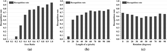

  

  Recognition rate, with respect to a axes ratio b/a, b major semi-axis length a and c and rotation $\theta$. The recognition rate here is the ratio of the correct detection images to the total number of images

As shown in Fig. 17b, the recognition rate is relatively low when the length of a is 10 pixels. With the length increasing, the recognition rate also goes up and reach the maximum point at a = 100.

The rotation angle also has influence on the recognition rate. The recognition rate reaches the minimum at the rotation angle = 40° (Fig. 17c). The low recognition rate is due to that the size of the arcs after the classification (Sect. 2.1) cannot satisfy the length constraint. For example, as shown in Fig. 18, when the rotation angle is 45°, the length of the arcs belonging to I, III is far less than those belonging to II, IV, which causes mistakable removing of the short arcs.

Fig. 18

An example of an oblique ellipse. The rotation angle of the ellipse will affect the length of arcs

• (7) Single Ellipse with Multiple Scales: When the ellipse target is small, the classified arcs are difficult to satisfy the size constraint, and the round-off errors become significant due to low resolution. In practical applications, upscaling the input image 1.5–2 times is a quick and effective way to solve such problems. However, since the proposed approach employs a series of control parameters, it is necessary to verify whether theses parameters can adapt to the scale changes. Synthetic dataset #2 is upscaled to 1.5 and 2 times of the original images, and the experimental results are shown in Fig. 16. It is evident that upscaling the detection image can improve the detection effect and reduce the false detection caused by axes length and rotation angle. Nevertheless, as the axes ratio is too small, such as 0.1, the improvement is not obvious. In general, upscaling the detection image 1.5–2 times can improve the detection effect, and the control parameters in the proposed method can be adapted to such scale change detection.

• (8) Images with No Ellipses The images with no ellipses are used to evaluate the filtering ability of the proposed method for interference lines. As shown in Fig. 19, the proposed method can effectively reduce the occurrence of false detection when there are line segments and noise interference in the image. The average number of false detections per image with each ${\mathcal{J}}$ is presented in Fig. 19g. As the line segments increase, the false detected ellipses of Fornaciari’s method gradually increase. However, the false detection of Jia’s method and the proposed method is obviously much less than that of Fornaciari’s method. Totally, there are seven false detected ellipses occurred by Jia’s method and two by our method in the 600 test images. We show all false detected ellipses in Fig. 19h.

  Fig. 19

  

  Testing on synthetic images which contain overlapping line segments and are corrupted by 4% salt-and-pepper noise. a–f Examples of detection results. The first row shows examples of the test image with the number of lines shown in the bottom right corner of the image. The second to fourth rows demonstrate the results detected by Fornaciari’s method, Jia’s method and our method, respectively. g Average number of false detections per image plotted against the number of overlapping line segments. h All false detections of our method across the 600 test images

• (9) Occluded Ellipses The detection ability of the proposed method for occluded ellipses is tested in this part. Some examples of detection results are shown in Fig. 20a. As observed, the proposed method cannot recognize the ellipses with large overlapped area, which leads to low recall rate. Nevertheless, a high detection precision is obtained, and the number of false detection is significantly lowered. As the number of occluded ellipses increases, the overlapped area of the ellipse increases gradually, which results in the poor detection and the decrease of F-measure (Fig. 20b). Meanwhile, there are more arcs to be processed, but our method still maintains a relatively fast detection speed, as shown in Fig. 20c.

  Fig. 20

  

  Testing on synthetic images containing occluded ellipses. a Examples of detection results. The first row shows examples of the test image with the number of occluded ellipses shown in the top left corner of the image. The second to fourth rows demonstrate the results detected by Fornaciari’s method, Jia’s method and our method, respectively. b F-measure and c execution time are plotted against the number of occluded ellipses. The values of the data in the figure are the average of 100 different synthetic images with the same number of ellipses

The proposed method is unable to detect the ellipse with one quadrant missing. However, in the detection scenario where there is no obvious occlusion on the elliptical target, the proposed method can work better than conventional methods. In the experiments, it is found that the proposed method can accurately identify the occluded ellipses in which each quadrant is not completely lost.

• (10) Half Ellipses Synthetic images (400 × 400) with half ellipse were generated to evaluate the limitation of the proposed method, and some examples are shown in Fig. 21. The experimental results show that the proposed method cannot detect such ellipses, which reflects the limitation of the proposed approach. Concretely, our method is unable to detect the ellipse with one quadrant missing, due to the requirement of providing four quadrant arcs in the arc grouping phase.

  Fig. 21

  

  Examples of half ellipses used in the experiment

• (11) Stretched Ellipses In Fig. 16, we plot the false detection distribution with axes ratio from 0.1 to 1. To intuitively demonstrate the detection results on the stretched ellipse, twenty-five ellipses are generated on a 1000 × 1000 image. The length of semi-major is set to 100, and the orientation of the ellipses is assigned randomly in the range sdpf. In addition, the axe ratio of the stretched ellipse is randomly distributed from 0.1 to 0.4. As observed in Fig. 22, the proposed method has fewer false detection. As the ellipse is too flat and the axes ratio is about 0.1, it is difficult to detect the ellipse by the proposed method. This is mainly due to the fact that the arcs in the flat ellipse cannot be accurately classified, which leads to the failure of subsequent grouping. As axes ratio increases to around 0.2, these stretched ellipses are accurately identified.

  Fig. 22

  

  Examples of stretched ellipses detection results. a original image. b–d Ellipses detected by Fornaciari’s method, Jia’s method and our method

• (12) Images of Different Sizes As shown in Fig. 23, when the image size is 100 × 100 or 200 × 200, the detection results of the three methods are worse. The reason is that the number of an ellipse edge pixels is too small to meet the fitting requirements. In this case, the image upsampling can be leveraged to improve the detection. With the image size increasing, F-measure does not fluctuate significantly. This is because the proposed method relies on the geometric properties of the ellipse to screen candidate arcs. When the size of an ellipse is too small, the strict size constraints will filter out the edge. With the increase in the arc size, the incidence of such false filtering will decrease.

  Fig. 23

  

  Comparative results under varying image sizes

• (13) Overlapping Ellipses Under Gaussian Noise In this experiment, 100 images with the size of 500 × 500 are generated. Each image contains six ellipses. The parameters of the ellipses obey the uniform random distribution, and center points are random located within the image. The lengths of semi-major and semi-minor axes are set randomly in the range $\left[ {50,100} \right]$, and the orientations of ellipses are assigned randomly in the range $\left[ {0^\circ ,90^\circ } \right]$. The intensity of the ellipses in the image is 0, and the intensity of the background is 255. Gaussian noise with 0 mean and standard deviations ranged from 0 to 80 is added to the gray values of each pixels in the image.

As shown in Fig. 24a, as the standard deviation of Gaussian noise increases, the detection results of the three ellipse detection methods gradually deteriorate. As shown in Fig. 24b, as the standard deviation of Gaussian noise increases to 70, Jia’s method is unable to identify ellipses. The proposed method and Fornaciari’s method cannot identify ellipses when the deviation increases to 80. Since the noise breaks the edge, the broken edges cannot satisfy the constraints of forming an ellipse. Nevertheless, the detection accuracy of the proposed method under Gaussian noise is relatively high.

Fig. 24

Experiment under Gaussian noise. a Examples of detection results. The first row shows examples of the test image. The mean value of Gaussian noise is zero. The standard deviation of Gaussian noise is shown in the bottom right corner of the image. The second to fourth rows demonstrate the results detected by Fornaciari’s method, Jia’s method and our method, respectively. b F-measure and c execution time are plotted against the standard deviation of Gaussian noise. The values of the data in the figure are the average of 100 different synthetic images

As the Gaussian standard deviation increases, the number of interference edges increases gradually, which increases the detection time. As shown in Fig. 24c, when the deviation increases to 50, the detection time becomes shorter. This is because most of the edges do not meet the constraints of forming an ellipse, and no time is spent on fitting and post-processing. In general, the proposed method maintains a relatively fast speed under the Gaussian noise.

5.4.2 Experimental results with real image datasets

• (1) Original Real Images The performance of the proposed method is compared against two state-of-the-art detection methods which have preferable detection affection and high detection speed. As shown in Table 4, the detection results of the proposed method on three classical datasets are not stable. This is because some objects of oval shapes like airship, irregular polygon and human faces are regarded as ellipses in the classical datasets. In industrial applications, these non-elliptical objects are often needed to be circumvented, since they would weaken the pertinence of elliptical target detection. The proposed method achieves accurate and stable detection on CMOS and phone datasets containing regular ellipses.

  Table 4 Result of our method compared with the-state-of-the-art methods on five real image datasets

We show the execution time for each processing steps in Table 5. The proposed method is more efficient than the current speed leading methods. Compared with the two conventional methods, for CMOS dataset, the execution time is reduced by 17.75% (from 50.53 to 41.56 ms) and 53.65% (from 89.66 to 41.56 ms), respectively, and for phone dataset, it is reduced by 16.32% (from 62.55 to 52.34 ms) and 48.07% (from 100.78 to 52.34 ms), respectively. For all the three methods, the most time-consuming step is grouping which is a combination process of three arcs (Fornaciari’s method and Jia’s method) or four arcs (proposed method). By using the size constraint, relative position constraint and tangent lines constraint, the interference edges are effectively filtered out and the grouping is greatly accelerated.

Table 5 Execution time (ms) for each step on CMOS dataset and phone dataset

Some detected examples on the five datasets are depicted in Figs. 25 and 26. For Fornaciari’s method and Jia’s method, there are more wrongly detected ellipses and undetected ellipses. The reason is that the parameter estimation strongly depends on the result of edge detection. Moreover, since the constraint of the ellipse is not strong enough, there will be more false detection. Some ellipses also cannot be detected by the proposed method, and it is mainly because large area occlusion or edge blurred.

Fig. 25

Examples of images in three classic datasets. The first two images are from Prasad dataset. The third and fourth images are from Fornaciari dataset #1. The rest two images are from Fornaciari dataset #2. a Original image, b canny edge map, c ellipses detected by the proposed method, d Fornaciari’s method and e Jia’s method

Fig. 26

Examples of images of CMOS dataset and phone dataset. The gray images of the first three lines come from CMOS dataset, and the color images come from phone dataset. a Original image, b canny edge map, c ellipses detected by the proposed method, d Fornaciari’s method and f Jia’s method

• (2) Real Image Under Salt-And-Pepper Noise We added salt-and-pepper noise to phone dataset with the noise rate from 2 to 20% with the step of 2% to test the robustness of the proposed method. As shown in Fig. 27, the F-measures for all three methods in the experiment show a downward trend as the noise rate increases. Accordingly, the precision increases and the recall decreases. Until the noise rate increases to 10%, three methods all have a high F-measure which are about 0.64, 0.65, 0.66 for proposed method, Jia’s method, Fornaciari’s method, respectively. When the noise rate is below 18%, the F-measure of proposed method is close to that of Jia’s method. However, if the noise rate is 20%, the detection of the proposed method becomes worse. This is mainly because that the elliptical edges are broken in small pieces by noise and cannot satisfy the size constraint or the geometric constraint.

  Fig. 27

  

  Detection results of Fornaciari’s method, Jia’s method and our method under salt-and-pepper noise with varying ratios of noise from 2 to 22% with the step 2%

All three methods in the experiment run faster with noise increasing because more edges were removed as interference lines in preprocessing. The proposed method still maintains relatively high detection speed in the experiment.

6 Application

In the industrial production, the ellipse detection can be used to locate the circle object for quality inspection and assembly. Therefore, the ellipse detection was also performed on the mechanical part images. Some of detection results are presented in Fig. 28. It can be seen that the proposed method can effectively extract the circular target on mechanical parts. After utilizing interference edge filtering and false detection removal, the detected ellipse edge coincides well with the actual circular hole edge, which can well support the hole location or aperture calculation.

Fig. 28

Application examples of ellipse detection for mechanical parts

7 Conclusions

In this paper, we proposed a fast and effective ellipse detection method, which is faster than the current speed leading detection method and performs better detection results. The proposed arc classification, interference edge removal, arc grouping and ellipse validation approaches can effectively improve the detection speed while reducing the number of false detections. The results of noise added experiments and multi-scale experiments demonstrate the robustness of the proposed method. The average execution time for the image in size of 300 × 400 taken by mobile phone is 52.34 ms, and the average value of F-measure is 0.745, which can meet the requirement of real-time detection.

The proposed method can significantly speed up the grouping procedure. However, it assumes that an ellipse has four arcs in different quadrants. Therefore, the ellipse will not be detected when large area of occlusion happens. In the detection scenario where there is no obvious occlusion on the elliptical target, the proposed method works better than the conventional methods. Several thresholds are utilized, which is not conductive to the optimization and stability of the algorithm. However, the proposed method can satisfy most of the actual detection condition. In the future, we will focus on reducing the number of thresholds and try to improve the stability of the algorithm.

References

Li, W., Shan, S., Liu, H.: High-precision method of binocular camera calibration with a distortion model. Appl. Optics 56(8), 2368–2377 (2017)
Da, F., Li, Q., Zhang, H., Fang, X.: Self-calibration using two same circles. Opt. Laser Technol. 44(6), 1924–1933 (2012)
Liu, C., Hu, W.: Ellipse fitting for imaged cross sections of a surface of revolution. Pattern Recognit. 48(4), 1440–1454 (2015)
Wang, Z., Wu, Z., Zhen, X., Yang, R., Xi, J., Chen, X.: A two-step calibration method of a large FOV binocular stereovision sensor for onsite measurement. Measurement 62(2), 15–24 (2015)
Wang, Z., Wu, Z., Zhen, X., Yang, R., Xi, J., Chen, X.: An onsite inspection sensor for the formation of hull plates based on active binocular stereovision. Proc. IMechE Part B: J. Eng. Manuf. 492(3), 887–896 (2014)
Zafari, S., Eerola, T., Sampo, J., Kalviainen, H., Haario, H.: Segmentation of overlapping elliptical objects in silhouette images. IEEE Trans. Image Process. 24(12), 5942–5952 (2015)
Duda, R.O., Hart, P.E.: Use of the Hough transformation to detect lines and curves in pictures. Commun. ACM 15(1), 11–15 (1972)
Helgason, S.: The radon transform, vol. 2. Birkhäuser, Boston (1999)
Ballard, D.H.: Generalizing the Hough transform to detect arbitrary shapes. Pattern Recognit. 13(2), 111–122 (1981)
McLaughlin, R.A.: Randomized Hough transform: improved ellipse detection with comparison. Pattern Recognit. Lett. 19(3), 299–305 (1998)
Kiryati, N., Eldar, Y., Bruckstein, A.M.: A probabilistic Hough transform. Pattern Recognit. 24(4), 303–316 (1991)
Kiryati, N., Kalviainen, H., Alaoutinen, S.: Randomized or probabilistic Hough transform: unified performance evaluation. Pattern Recognit. Lett. 21(13), 1157–1164 (2000)
Lu, W., Tan, J.: Detection of incomplete ellipse in images with strong noise by iterative randomized Hough transform (IRHT). Pattern Recognit. 41(4), 1268–1279 (2008)
Chia, A.Y., Rahardja, S., Rajan, D., Leung, M.K.: A split and merge based ellipse detector with self-correcting capability. IEEE Trans. Image Process. 20(7), 1991–2006 (2010)
Lu, T., Hu, W., Liu, C., Yang, D.: Effective ellipse detector with polygonal curve and likelihood ratio test. Comput. Vis. IET 9(6), 914–925 (2015)
Chen, S., Xia, R., Zhao, J., Chen, Y., Hu, M.: A hybrid method for ellipse detection in industrial images. Pattern Recognit. 68(18), 82–98 (2017)
Fitzgibbon A.W., Pilu M., Fisher R.B.: Direct least square fitting of ellipses. In: Presented at ICPR (1996). http://ieeexplore.ieee.org/document/546029/
Prasad, D.K., Leung, M.K.H., Quek, C.: ElliFit: an unconstrained, non-iterative, least squares based geometric ellipse fitting method. Pattern Recognit. 46(5), 1449–1465 (2013)
Liang, J., Wang, Y., Zeng, X.: Robust ellipse fitting via half-quadratic and semidefinite relaxation optimization. IEEE Trans. Image Process. 24(11), 4276–4286 (2015)
Mulleti, S., Seelamantula, C.S.: Ellipse fitting using the finite rate of innovation sampling principle. IEEE Trans. Image Process. 25(3), 1451–1464 (2016)
Liu, D., Wang, Y., Tang, Z., Lu, X.: A robust circle detection algorithm based on top-down least-square fitting analysis. Comput. Electr. Eng. 40(4), 1415–1428 (2014)
Wang Y., He Z., Liu X., Tang Z., Li L.: A fast and robust ellipse detector based on top-down least-square fitting. In: Presented at BMVC (2015). http://www.bmva.org/bmvc/2015/papers/paper156/abstract156.pdf
Prasad, D.K., Leung, M.K., Cho, S.Y.: Edge curvature and convexity based ellipse detection method. Pattern Recognit. 45(9), 3204–3221 (2012)
Fornaciari, M., Prati, A., Cucchiara, R.: A fast and effective ellipse detector for embedded vision applications. Pattern Recognit. 47(11), 3693–3708 (2014)
Jia, Q., Fan, X., Luo, Z., Song, L., Qiu, T.: A Fast ellipse detector using projective invariant pruning. IEEE Trans. Image Process. 26(8), 3665–3679 (2017)
Jin, R., Owais, H.M., Lin, D., Song, T., Yuan, Y.: Ellipse proposal and convolutional neural network discriminant for autonomous landing marker detection. J. Field Robot. 36(1), 6–16 (2019)
Dong, H., Prasad, D.K., Chen, I.: Accurate detection of ellipses with false detection control at video rates using a gradient analysis. Pattern Recognit. 81, 112–130 (2018)
Pătrăucean V., Gurdjos P., Gioi R.G.V.: A parameterless line segment and elliptical arc detector with enhanced ellipse fitting. In: Presented at ECCV (2012). https://springerlink.bibliotecabuap.elogim.com/chapter/10.1007/978-3-642-33709-3_41
Pătrăucean, V., Gurdjos, P., Gioi, R.G.V.: Joint A contrario ellipse and line detection. IEEE Trans. Pattern Anal. Mach. Intell. 39(4), 788–802 (2017)
Liu Y., Xie Z., Wang B., Liu H., Jing Z., Huang C.: A practical detection of non-cooperative satellite based on ellipse fitting. In: Presented at ICMA (2016). http://ieeexplore.ieee.org/document/7558793/
Canny, J.: A computational approach to edge detection. IEEE Trans. Pattern Anal. Mach. Intell. 8(6), 679–698 (1986). https://doi.org/10.1109/TPAMI.1986.4767851
Freeman, H.: Shapira R: determining the minimum-area encasing rectangle for an arbitrary closed curve. Commun. ACM 18(7), 409–413 (1975)
Dorrie, B., Bydavidantin, T.: 100 Great problems of elementary mathematics, p. 264. Dover, New York (1965)
Prasad, D.K., Leung, M.K., Quek, C., Brown, M.S.: DEB: definite error bounded tangent estimator for digital curves. IEEE Trans. Image Process. 23(10), 4297–4310 (2014)
Jaccard, P.: The distribution of flora in the alpine zone. New Phytol. 11(2), 37–50 (1912)
Acknowledgements
This work was supported in part by the National Natural Science Foundation of China under Grant 51935009 and U1608256, in part by National Science and Technology Major Project of the Ministry of Science and Technology of China under Grant 2018ZX04020-001, and in part by the Natural Science Foundation of Zhejiang Province under Grant Y19E050078. The authors would like to thank Dr. Fornaciari and Dr. Fan for providing their executables and insights. The authors also thank Dr. Prasad and Dr. Fornaciari for providing their experimental datasets.
Author information
Authors and Affiliations
Corresponding author
Additional information
Publisher's Note
Springer Nature remains neutral with regard to jurisdictional claims in published maps and institutional affiliations.
Rights and permissions
About this article
Cite this article
Liu, Z., Liu, X., Duan, G. et al. A real-time and precise ellipse detector via edge screening and aggregation. Machine Vision and Applications 31, 64 (2020). https://doi.org/10.1007/s00138-020-01113-1
Received:
Revised:
Accepted:
Published:
DOI: https://doi.org/10.1007/s00138-020-01113-1