Regularity of solutions to Kolmogorov equation with Gilbarg–Serrin matrix

Abstract

In ${\mathbb {R}}^d$, $d \ge 3$, consider the divergence and the non-divergence form operators

$$\begin{aligned}&-\Delta - \nabla \cdot (a-I) \cdot \nabla + b \cdot \nabla , \\&- \Delta - (a-I) \cdot \nabla ^2 + b \cdot \nabla , \end{aligned}$$

where the second-order perturbations are given by the matrix

$$\begin{aligned} a-I=c|x|^{-2}x \otimes x, \quad c>-1. \end{aligned}$$

The vector field $b:{\mathbb {R}}^d \rightarrow {\mathbb {R}}^d$ is form-bounded with form-bound $\delta >0$. (This includes vector fields with entries in $L^d$, as well as vector fields having critical-order singularities.) We characterize quantitative dependence on c and $\delta$ of the $L^q \rightarrow W^{1,qd/(d-2)}$ regularity of solutions of the corresponding elliptic and parabolic equations in $L^q$, $q \ge 2 \vee ( d-2)$.

1 Introduction

1. In this paper, we are concerned with the second-order perturbations of $-\Delta$,

$$\begin{aligned}&\begin{array}{c} -\Delta - \nabla \cdot (a-I) \cdot \nabla , \\ -\Delta - (a-I) \cdot \nabla ^2, \end{array}\\&a_{ij}(x):=\delta _{ij}+c|x|^{-2}x_ix_j, \quad c>-1. \nonumber \end{aligned}$$

(1)

These are model examples of divergence/non-divergence form operators that are not accessible by classical means such as the parametrix [8, 19, Ch. IV]. Although the matrix a is discontinuous at the origin, it is uniformly elliptic, so, by the De Giorgi–Nash theory, solution $u \in W^{1,2}({\mathbb {R}}^d)$ to the elliptic equation $(\mu -\nabla \cdot a \cdot \nabla ) u = f$, $\mu >0$, $f \in L^p\cap L^2$, $p \in ]\frac{d}{2},\infty [$, is in $C^{0,\gamma }$, where the Hölder continuity exponent $\gamma \in ]0,1[$ depends only on d and c. The operators (1) and their modifications have been studied by many authors in order to make more precise the relationship between the regularity properties of the solutions to the corresponding parabolic and elliptic equations and the continuity properties of the matrix, see [1, 3, 5, 18, Ch. 1.2], [7, 9, 20,21,22,23,24,25,26] and references therein. In fact, there is a quantitative dependence of the regularity properties of solutions on the value of c. In this sense, the matrix a has a critical-order discontinuity at the origin.

The critical-order perturbations of $-\Delta$ and its generalizations have been the subject of intensive study over the past few decades as they reveal otherwise inaccessible aspects of the theory of the unperturbed operator. For example, consider the Schrödinger operator $-\Delta - V_0$, $V_0(x)=\delta \frac{(d-2)^2}{4}|x|^{-2}$, on ${\mathbb {R}}^d$, $d \ge 3$. If $0<\delta < 1$, then the self-adjoint operator realization $H^-$ of $-\Delta - V_0$ on $L^2 \equiv L^2({\mathbb {R}}^d)$ is defined as the (minus) generator of a $C_0$ semigroup $e^{-tH^-}=s{\text{- }}L^2{\text{- }}\lim _{\varepsilon \downarrow 0} e^{-tH^-(V_{\varepsilon })}$, $V_{\varepsilon }(x)=\delta \frac{(d-2)^2}{4}|x|_\varepsilon ^{-2}$, $|x|_\varepsilon ^{2}:=|x|^2+\varepsilon$, $\varepsilon >0$. For $\delta >1$, however, by the celebrated result of [4] (see also [10]),

$$\begin{aligned} \lim _{\varepsilon \downarrow 0} e^{-tH^-(V_\varepsilon )}u_0(x)=\infty , \quad t>0, \quad x \in {\mathbb {R}}^d, \quad u_0 \ge 0,\; u_0 \not \equiv 0, \end{aligned}$$

i.e., all positive solutions explode instantly at any point. This phenomenon is not observable for any $V_0=\delta V$, $V \in L^{\frac{d}{2}}$, regardless of how large $\delta >0$ is (in this sense, the class $L^{\frac{d}{2}}$ does not contain potentials having critical-order singularities). The perturbations $\nabla \cdot (a-I) \cdot \nabla$, $(a-I)\cdot \nabla ^2$, $a-I=c|x|^{-2}x \otimes x$, of $-\Delta$ can be viewed as the second-order analogues of the critical potential $V_0(x)=\delta \frac{(d-2)^2}{4}|x|^{-2}$.

Our goal is to determine to what extent adding $\nabla \cdot (a-I) \cdot \nabla$, $(a-I)\cdot \nabla ^2$ affects the perturbation-theoretic and the regularity properties of $-\Delta$. Our interest is motivated by applications to diffusion processes, and so we restrict our study to the first-order perturbations of (1).

2. The following result concerning the special case $a=I$ (i.e., $c=0$) will serve as the point of departure. Consider on ${\mathbb {R}}^d$, $d \ge 3$, the Kolmogorov operator

$$\begin{aligned} -\Delta + b \cdot \nabla , \quad b:{\mathbb {R}}^d \rightarrow {\mathbb {R}}^d. \end{aligned}$$

We will need the following

Definition

A measurable vector field $b:{\mathbb {R}}^d \rightarrow {\mathbb {R}}^d$ is said to be form-bounded (with respect to $-\Delta$) if $|b| \in L^2_{\mathrm{loc}}$ and there exist constants $\delta >0$ and $\lambda =\lambda _\delta \ge 0$ such that

$$\begin{aligned} \Vert |b|(\lambda -\Delta )^{-\frac{1}{2}}\Vert _{2\rightarrow 2}\le \sqrt{\delta } \end{aligned}$$

(write $b \in \mathbf {F}_\delta$).

Here and below, $\Vert \cdot \Vert _{p \rightarrow q}$ denotes the $\Vert \cdot \Vert _{L^p \rightarrow L^q}$ operator norm.

The condition $b \in \mathbf {F}_\delta$ is equivalent to the quadratic form inequality

$$\begin{aligned} \langle b f, b f\rangle \le \delta \langle \nabla f, \nabla f \rangle + c_\delta \langle f,f\rangle , \quad \text { for all } f \in W^{1,2} \end{aligned}$$

for a constant $c_\delta$ $(=\lambda \delta )$, where, from now on,

$$\begin{aligned} \langle h\rangle :=\int _{{\mathbb {R}}^d} h(x)dx, \quad \langle h,g\rangle :=\langle h\bar{g}\rangle . \end{aligned}$$

The constant $\delta$ is called the form-bound of b. It measures the size of critical singularities of the vector field, see examples below.

It is clear that

$$\begin{aligned} b_1 \in \mathbf {F}_{\delta _1}, b_2 \in \mathbf {F}_{\delta _2} \quad \Rightarrow \quad b_1+b_2 \in \mathbf {F}_\delta , \qquad \sqrt{\delta }:=\sqrt{\delta _1}+\sqrt{\delta _2}. \end{aligned}$$

Examples

The class of form-bounded vector fields $\mathbf {F}_\delta$ contains vector fields b with $|b| \in L^d + L^\infty$ (i.e., $b=b_1+b_2$, where $|b_1| \in L^d$, $|b_2| \in L^\infty$), with $\delta >0$ that can be chosen arbitrarily small (by Sobolev’s inequality).

The class $\mathbf {F}_\delta$ also contains vector fields having critical-order singularities. For example, by Hardy’s inequality, the vector field

$$\begin{aligned} b(x):=\sqrt{\delta }\frac{d-2}{2}|x|^{-2}x, \quad \delta >0, \end{aligned}$$

having a model critical-order singularity at the origin, is contained in $\mathbf {F}_\delta$ (with $\lambda =0$). More generally, the class $\mathbf {F}_\delta$ contains vector fields b with |b| in $L^{d,\infty } + L^\infty$ (the weak $L^d$ class, by Strichartz’ inequality [16]), the Campanato–Morrey class or the Chang–Wilson–Wolff class [6], with $\delta$ depending on the norm of |b| in these classes.

For every $\varepsilon >0$, one can find $b \in \mathbf {F}_\delta$ such that $|b| \not \in L^{2+\varepsilon }_{\mathrm{loc}}$, e.g., consider a vector field b with

$$\begin{aligned} |b(x)|^2=C\frac{\mathbf {1}_{B(0,1+\kappa )} - \mathbf {1}_{B(0,1-\kappa )}}{\big | |x|-1\big |^{-1}(-\ln \big ||x|-1\big |)^\alpha }, \quad \alpha >1, \quad 0<\kappa <1. \end{aligned}$$

See, e.g.,  [11, Sect. 4] for other examples and more detailed discussion concerning the class $\mathbf {F}_\delta$.

Here is our point of departure. By [15, Lemma 5], for $b \in \mathbf {F}_\delta$ with $\delta <1 \wedge \bigl (\frac{2}{d-2}\bigr )^2$ and $q \in [2 \vee (d-2),\frac{2}{\sqrt{\delta }}[$ the solution u to the elliptic equation

$$\begin{aligned} \big (\mu +\Lambda _q(b)\big )u=f, \quad f \in L^q, \end{aligned}$$

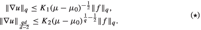
where $\Lambda _q(b)$ is an operator realization of $-\Delta + b\cdot \nabla$ in $L^q$ as the (minus) generator of a positivity preserving $L^\infty$ contraction $C_0$ semigroup (see details in Sect. 3), satisfies

for all $\mu >\mu _0$, where constants $\mu _0=\mu _0(d,q,\delta )>0$, $K_i=K_i(d,q,\delta )$, $i=1,2$. In particular, if additionally $q>d-2$, then by the Sobolev embedding theorem u is in $C^{0,\gamma }$ (possibly after change on a measure zero set) with Hölder continuity exponent $\gamma =1-\frac{d-2}{q}$.

3. In our main result, Theorem 2, we show that the perturbation $-\nabla \cdot (a-I) \cdot \nabla$ of $-\Delta$ preserves, under appropriate assumptions on c, the properties of $-\Delta$ that allow to establish estimates ($*$) for $u=\big (\mu +\Lambda _q(a,b)\big )^{-1}f$, where $\Lambda _q(a,b)$ is an operator realization of the formal operator

$$\begin{aligned} -\Delta - \nabla \cdot (a-I) \cdot \nabla + b \cdot \nabla , \qquad b \in \mathbf {F}_\delta \end{aligned}$$

in $L^q$ as the (minus) generator of a positivity preserving $L^\infty$ contraction $C_0$ semigroup, constructed as the limit of the semigroups corresponding to smooth approximations of a, b. The existing literature on $-\Delta - \nabla \cdot (a-I) \cdot \nabla + b \cdot \nabla$ dealing with discontinuous/locally unbounded coefficients, provides a detailed regularity theory of this operator in the case $a=I+c|x|^{-2}(x \otimes x)$ and $b(x)=c|x|^{-2}x$, see [5, 7, 20,21,22,23,24]. In the present paper, we are dealing with a substantially larger class of singular drifts b. Our results thus do not depend on the specific structure of b such as differentiability or symmetry, and, in fact, follow from the a priori estimates ($*$) for solutions to the corresponding elliptic equations with smoothed out coefficients.

Now, define vector field $\nabla a$ by $(\nabla a)_k := \sum _{i=1}^d \nabla _i a_{ik}$, $1 \le k \le d$, where, from now on, $\nabla _i:=\partial _{x_i}$. Then $\nabla a=c(d-1)|x|^{-2}x$ , so by Hardy’s inequality $\nabla a \in \mathbf {F}_\delta$, $\delta _a=\frac{4c^2(d-1)^2}{(d-2)^2}$. We construct an operator realization in $L^q$ of the non-divergence form (formal) operator

$$\begin{aligned} -a \cdot \nabla ^2 + b \cdot \nabla \equiv -\sum _{i,j=1}^d a_{ij}(x) \nabla _i \nabla _j + \sum _{k=1}^d b_k(x) \nabla _k, \quad b \in \mathbf {F}_{\delta _1} \end{aligned}$$

as $\Lambda _q(a,\nabla a + b)$ (we have $-a \cdot \nabla ^2 + b \cdot \nabla \equiv - \nabla \cdot a \cdot \nabla + (\nabla a+b) \cdot \nabla$). As a result, we can characterize the quantitative dependence of the regularity properties of $u = (\mu +\Lambda _q(a,\nabla a + b))^{-1}f$, $f \in L^q$, on $c,d,q, \mu$ and $\delta$, see Corollary 3. In this regard, we note that the class of admissible first-order perturbations $b \cdot \nabla$, $b \in \mathbf {F}_{\delta }$ of $-a \cdot \nabla ^2$ cannot be achieved on the basis of the Krylov–Safonov a priori estimates [17, Ch. 4.2]. (We note that the operator $-a\cdot \nabla ^2$ with $\partial _{x_k}a_{ij} \in L^{d,\infty }$ has been studied earlier in [2], see also [3].)

Concerning the application of ($*$) to establishing the $C^{0,\gamma }$ continuity of u, we note the following. Let $d \ge 4$. In the proof of Theorem 2, we establish a stronger than ($*$) estimate:

$$\begin{aligned} \Vert \nabla |\nabla u|^{\frac{q}{2}}\Vert _2^2 \le K \Vert f\Vert ^q_q \end{aligned}$$

(and so $u \in C^{0,\gamma }$, $\gamma =1-\frac{d-2}{q}$). We do not appeal, for the purpose of establishing Hölder continuity of u, to $W^{2,r}$ estimates on u for a large r. In fact, the condition $b \in \mathbf {F}_\delta$, $\delta <1$ yields only $u \in W^{2,2}$. The latter allows to conclude that u is Hölder continuous only in dimension $d=3$.

In Theorem 2, we tried to find the least restrictive assumptions on c and $\delta$ (a measure of discontinuity of matrix a and a measure of singularity of vector field b, respectively), permitted by the method, such that the estimates ($*$) hold for a $b \in \mathbf {F}_\delta$. (We emphasize that our result is not of Cordes type.) The weaker result that there exist sufficiently small c and $\delta$ such that the estimates ($*$) are valid (still not accessible by the existing results prior to our work) can be obtained with considerably less effort by following the proof and discarding the corresponding multiples of c and $\delta$.

The question of optimality of our assumptions on c and $\delta$ in Theorem 2 is difficult. Even in the case $c=0$, it is not yet clear whether the corresponding assumption on $\delta$ (i.e., $\delta <1 \wedge \frac{4}{(d-2)^2}$), although dictated by the method, is optimal. (We remark that the constant $\frac{4}{(d-2)^2}$, incidentally, coincides with the constant in Hardy’s inequality for $d \ge 4$.) In this regard, we note the following:

• 1. We believe that the examples showing the optimality of the assumptions on c and $\delta$ in Theorem 2 (at least in the limiting cases discussed in the fourth remark after Theorem 2) could be obtained once one fully exploits the method, e.g., in the context of the problem of constructing the corresponding diffusion process. (In this regard, we note [12, Example 1].)

• 2. In [23, 24], the authors constructed an operator realization $Q_p$ of $-\Delta - \nabla \cdot (a-I)\cdot \nabla + b \cdot \nabla$ in $L^p$ for the model vector field $b(x)=c|x|^{-2}x$ and characterized the domain of $Q_p$, establishing $W^{1,p}$ and $W^{2,p}$ regularity of any u in the domain of $Q_p$. The results in [23, 24] do not follow as a special case of Theorem 2 if we take there $b(x)=c|x|^{-2}x$. In fact, for this vector field, one can modify our method to take into account the sign of the divergence of b (cf.  [11, Corollaries 4.9–4.11]); however, this still does not allow to obtain as a special case the related result in [23, 24].

We note that having a complete characterization of the domain of (an operator realization of) $-\nabla \cdot a \cdot \nabla$ in $L^q$ for some q does not help on its own to characterize regularity of the domain of $-\nabla \cdot a \cdot \nabla + b \cdot \nabla$, $b \in \mathbf {F}_\delta$ in $L^q$ (as is already apparent in the case $a=I$ discussed above).

The method of this paper is suited to treat second-order perturbations $-\nabla \cdot (a-I)\cdot \nabla$, $-(a-I) \cdot \nabla ^2$ of $-\Delta$ more general than $a-I=c|x|^{-2}x \otimes x$, for example, $a-I=v \otimes v$, where a bounded $v:{\mathbb {R}}^d \rightarrow {\mathbb {R}}^d$, $v \in W^{1,2}_{\mathrm{loc}}({\mathbb {R}}^d,{\mathbb {R}}^d)$ satisfies

$$\begin{aligned} \big (\sum _k (\nabla v_k)^2\big )^{\frac{1}{2}} \in \mathbf {F}_\delta \end{aligned}$$

(2)

(although not distinguishing between positive and negative c). Our method also admits extension to

$$\begin{aligned}&a_{ij}(x)=\delta _{ij}+\sum _lc_l\kappa _{ij}(x - y^l), \quad \kappa _{ij}(x)=|x|^{-2}{x_ix_j}, \\&c_+:=\sum _{c_l>0}c_l<\infty ,\quad c_-:=\sum _{c_l<0}c_l >-1, \end{aligned}$$

where $\{y^l\} \subset {\mathbb {R}}^d$. Let us also note that arguments in this paper can be transferred without significant changes from ${\mathbb {R}}^d$ to the ball B(0, 1).

After this paper was written [13], in subsequent paper [14] we constructed and investigated the diffusion process corresponding to $-a \cdot \nabla ^2 + b \cdot \nabla$ with a as in (2) using analogues of estimates ($*$), although valid, if restricted to $a=I+c|x|^{-2}x\otimes x$, under substantially more restrictive assumptions on c than in the present paper.

Outline of the method Let us give an informal outline of the proof of Theorem 2, i.e., estimates ($*$) for solution u to the elliptic equation $(\mu -\nabla \cdot a \cdot \nabla + b \cdot \nabla )u=f$, $\mu >0$, $f \in L^q$, $q > d-2$ (sufficiently close to $d-2$).

Step 1: The basic equality. We multiply the equation by carefully chosen “test function” and integrate to obtain the basic equality

$$\begin{aligned} \mu \Vert \nabla u\Vert _q^q + I_q + (q-1)J_q = [\dots ] + \Vert f\Vert _q^q, \quad J_q:=\Vert \nabla |\nabla u|^{\frac{q}{2}}\Vert _2^2. \end{aligned}$$

(BE)

The term $I_q$ is greater than $J_q$, so if we replace it by $J_q$ we arrive at

Step 2: The principal inequality. The terms $[\dots ]$ in the RHS of (BE) are estimated from above by $\kappa J_q$ with a sufficiently small coefficient $\kappa >0$ (using the structure of the matrix a and the condition $b \in \mathbf {F}_\delta$). Thus, we obtain from (BE)

$$\begin{aligned} \mu \Vert \nabla u\Vert _q^q + (q-1)J_q \le \kappa J_q + C\Vert f\Vert ^q_q, \end{aligned}$$

and so if $\kappa <q-1$ ($\Leftrightarrow$ our assumptions on a, b are satisfied) then we obtain the principal inequality

$$\begin{aligned} \mu \Vert \nabla u\Vert _q^q + \eta J_q \le C\Vert f\Vert ^q_q, \quad \eta >0. \end{aligned}$$

Step 3: The sought estimates ($*$) on u now follow from the previous inequality by applying the Sobolev embedding theorem to $J_q$.

Structure of the paper In Sect. 2, we state our results in detail. In Sect. 3, we illustrate the use of our method by applying it first to operator $-\Delta + b \cdot \nabla$, $b \in \mathbf {F}_\delta$. In Sect. 4, we prove our main result, Theorem 2 concerning the divergence form operator $-\nabla \cdot a \cdot \nabla + b \cdot \nabla$.

2 Main results

1. In what follows, we consider $C^\infty$ smooth approximation of the matrix $a(x)=I+c|x|^{-2}x \otimes x$ by

$$\begin{aligned} a^\varepsilon =(a^\varepsilon _{ij}), \quad 1 \le i,j \le d, \end{aligned}$$

where

$$\begin{aligned} a^\varepsilon _{ij}:=\delta _{ij}+c|x|^{-2}_\varepsilon x_ix_j, \quad |x|_\varepsilon :=\sqrt{|x|^2+\varepsilon }, \quad \varepsilon >0. \end{aligned}$$

For a given vector field $b \in \mathbf {F}_{\delta }$, we consider its $C^\infty$ smooth approximation defined by

$$\begin{aligned} b_n := c_n\gamma _{\epsilon _n} *{\mathbf {1}}_n b, \quad n \ge 1, \quad c_n \uparrow 1, \end{aligned}$$

(3)

where ${\mathbf {1}}_n$ is the indicator of $\{x \in {\mathbb {R}}^d \mid \; |x| \le n, |b(x)| \le n \}$, $\gamma _{\epsilon }$ is the K. Friedrichs mollifier, for appropriate $\epsilon _n \downarrow 0$ and $c_n \uparrow 1$ so that $b_n \in \mathbf {F}_\delta$ for all $n \ge 1$ with $\lambda \ne \lambda (n)$, see Remark 2 for details.

In the course of the proof of Theorem 2, we will first prove the required regularity estimates ($*$) for solution $u^{\varepsilon ,n}$ to the elliptic equation with smooth coefficients $(\mu -\nabla \cdot a^\varepsilon \cdot \nabla + b_n \cdot \nabla )u^{\varepsilon ,n}=f$, $f \in C_c^\infty$, $\mu \ge \mu _0$ for constants $\mu _0>0$ and $K_l$, $l=1,2$ independent of $\varepsilon$, n. Taking $\varepsilon \downarrow 0$ and $n \rightarrow \infty$, we will establish estimates ($*$) for solution u to the equation $(\mu -\nabla \cdot a \cdot \nabla + b \cdot \nabla )u=f$. However, first we need to specify in what sense the operator $-\nabla \cdot a \cdot \nabla + b \cdot \nabla$ is defined; we will also need the corresponding convergence result; see Theorem 1.

Recall that there is a unique self-adjoint operator $A\equiv A_2 \ge 0$ in $L^2$ associated with the sesquilinear form $\mathfrak {t}[u,v]:=\langle \nabla u \cdot a \cdot \nabla \bar{v} \rangle$, $D(\mathfrak {t})=W^{1,2}$:

$$\begin{aligned} D(A) \subset D(\mathfrak {t}) \quad \text { and } \quad \langle Au,v\rangle =\mathfrak {t}[u,v],\;\;u \in D(A),v \in D(\mathfrak {t}). \end{aligned}$$

The operator $-A$ is the generator of a positivity preserving $L^\infty$ contraction $C_0$ semigroup $T^t_2 \equiv e^{-tA}$, $t \ge 0$, on $L^2$. Then, since $T_2^t$ is a $L^\infty$ contraction, $T^t_q:=\big [T^t_2\upharpoonright _{L^q \cap L^2}\big ]_{L^q \rightarrow L^q}^{\mathrm{\mathrm{clos}}}$ determines by interpolation a contraction $C_0$ semigroup in $L^q$ for all $q \in [2,\infty [$ and hence, by self-adjointness, for all $q \in ]1,\infty [$. The (minus) generator $A_q$ of $T^t_q \,(\equiv e^{-tA_q})$ is an operator realization of the formal operator $\nabla \cdot a \cdot \nabla$ on $L^q$, $q \in ]1,\infty [$.

In what follows, given a Banach space Y and a sequence of bounded linear operators $T_n, T: Y \rightarrow Y$, we write $T=s\text{- } Y \text{- }\lim _n T_n$ if $Tf=\lim _n T_nf$ in Y for every $f \in Y$.

We will need

Theorem 1

Let $d \ge$3. Let $b \in \mathbf {F}_{\delta }$ with $\delta _1:=[1 \vee (1+c)^{-2}]\,\delta < 4$. Let $q > \frac{2}{2-\sqrt{\delta _1}}$. The following is true.

• (i) There exists the limit

  $$\begin{aligned} s\text{- }L^q\text{- }\lim _{n\rightarrow \infty } e^{-t \Lambda _q(a,b_n)} \quad (\text {locally uniformly in } t \ge 0), \end{aligned}$$

  where $\Lambda _q(a, b_n)=A_q + b_n \cdot \nabla$, $D(\Lambda _q(a, b_n))=D(A_q)$, and determines a positivity preserving, $L^\infty$ contraction, quasi-contraction $C_0$ semigroup $e^{-t \Lambda _q(a,b)}$ in $L^q$. Its (minus) generator $\Lambda _q(a,b)$ is an appropriate operator realization of the formal operator $-\nabla \cdot a \cdot \nabla + b \cdot \nabla$ in $L^q$.

• (ii)
  $$\begin{aligned} \Vert e^{-t\Lambda _q(a,b)}\Vert _{q \rightarrow q} \le e^{\omega _q t}, \quad t>0, \quad \omega _q:=\frac{\lambda \delta _1}{2(q-1)}. \end{aligned}$$
• (iii)
  $$\begin{aligned} (\mu +\Lambda _q(a,b))^{-1} = s\text{- }L^q\text{- }\lim _{n \rightarrow \infty }\lim _{\varepsilon \downarrow 0} (\mu +\Lambda _q(a^\varepsilon ,b_n))^{-1}, \quad \text { for all } \mu >\omega _q, \end{aligned}$$

  where $\Lambda _q(a^\varepsilon , b_n)=-\nabla \cdot a^\varepsilon \cdot \nabla + b_n \cdot \nabla$, $D(\Lambda _q(a^\varepsilon , b_n))=W^{2,q}$.

Proof

Assertions (i), (ii) are a special case of [11, Theorem 4.2] or of [11, Theorem 4.3] (both valid for an arbitrary uniformly elliptic matrix a).

Proof of (iii). By [11, Theorem 4.6], for every $n \ge 1$,

$$\begin{aligned} (\mu +\Lambda _q(a,b_n))^{-1} = s\text{- }L^q\text{- }\lim _{\varepsilon \downarrow 0} (\mu +\Lambda _q(a^\varepsilon ,b_n))^{-1}. \end{aligned}$$

It remains to apply (i). $\square$

2. We are in position to state the main result of the paper. Let us introduce the following quantities:

$$\begin{aligned}&L_1(c,\delta ,d):=c\biggl [\frac{1}{2(d-1)}+\frac{\sqrt{\delta }}{2}(d-2)(d+4) \biggr ] + \biggl [\frac{(d-2)^2\delta }{4}+\frac{(d-4)(d-2)}{2}\sqrt{\delta }\biggr ], \\&L_2(c,\delta ,d):=-c\biggl [2d-4 + \frac{\sqrt{\delta }}{2}(d-2)(d+4) \biggr ] + \biggl [\frac{(d-2)^2\delta }{4}+\frac{(d-4)(d-2)}{2}\sqrt{\delta }\biggr ]. \end{aligned}$$

Clearly, $L_1$, $L_2$ are small if c, $\delta$ are small.

Theorem 2

(The operator $-\nabla \cdot a \cdot \nabla + b \cdot \nabla$). Let $d \ge 3$, $a(x)=I+c|x|^{-2}x \otimes x$, $c>-1$, and $b \in \mathbf {F}_\delta$, $\delta >0$.

• (i) Let $d\ge 4$. Assume that c, $\delta$ (i.e., a measure of discontinuity of matrix a and a measure of singularity of vector field b, respectively) satisfy $[1 \vee (1+c)]\sqrt{\delta }<2-\frac{2}{d-2}$ and one of the following conditions:

• (1) $c>0$ and $1+c\big (1-\frac{1}{2(d-1)}-\frac{(d-2)\sqrt{\delta }}{4}\big ) > 0$, and

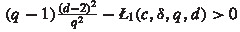
  $$\begin{aligned} L_1(c,\delta ,d)<d-3. \end{aligned}$$

• (2) $-1<c<0$ and $1+c\big (1+\frac{(d-2)\sqrt{\delta }}{4}\big ) > 0$, and

  $$\begin{aligned} L_2(c,\delta ,d)<d-3. \end{aligned}$$

  Then for every $q>d-2$ sufficiently close to $d-2$ there exist constants $\mu _0=\mu _0(d,q,c,\delta )\,(\ge \omega _q)$ and $K_l=K_l(d,q,c,\delta )$ ($l=1,2$) such that, for all $\mu >\mu _0$ and $f \in L^q$, $u:=(\mu +\Lambda _q(a,b))^{-1}f \in W^{1,q} \cap W^{1,\frac{qd}{d-2}}$ and satisfies

  

• (ii) Let $d\ge 3$. Assume that c, $\delta$ satisfy $\delta < 1 \wedge (1+c)^{2}$ and one of the following conditions holds:

  $$\begin{aligned} c>0,&\qquad 1-c\biggl [\frac{4}{(d-2)^2}+\sqrt{\delta }\biggl (2\frac{d+3}{d-2}+1 \biggr )\biggr ]-\delta>0, \\&\text { or } \\ -1<c<0,&\qquad 1-|c|\biggl [1+\frac{4(d-1)}{(d-2)^2}+\sqrt{\delta }\biggl (2\frac{d+3}{d-2}+1 \biggr )\biggr ]-\delta >0. \end{aligned}$$

  Then ($\star$) holds with $q=2$ and moreover, $u \in W^{2,2}$.

Remarks

• 1. In Theorem 2, if $c=0$, then the assumptions on $\delta$ are reduced to $\delta <1 \wedge \frac{4}{(d-2)^2}$, so we recover the result in [15, Lemma 5].

• 2. In assertion (i) of Theorem 2, we could also include $d = 3$, $q \ge 2$; however, for $d=3$ assertion (ii) yields a stronger regularity result $u \in W^{2,2}$.

• 3. Following closely the proof of Theorem 2, one can obtain conditions on c, $\delta$ and $q>d-2$ that provide estimates ($\star$), not necessarily assuming that q is close to $d-2$. In this case, we would have to replace hypothesis 1) in Theorem 2, i.e., “$1+c\big (1-\frac{1}{2(d-1)}-\frac{(d-2)\sqrt{\delta }}{4}\big ) > 0$ and $L_1(c,\delta ,d)<d-3$,” by “$1+c(1-\frac{1}{2(d-1)}-\frac{q\sqrt{\delta }}{4})$ and ,” where is defined in the proof of Theorem 2. Similarly for hypothesis 2). We opt to work with q close to $d-2$ to keep the assumptions of the theorem tractable.

• 4. In the assumptions of Theorem 2, the second estimate in ($\star$) and the Sobolev embedding theorem yield that u is Hölder continuous (possibly after a change on a measure zero set). For the illustration purposes, let us state the corresponding result in the case when either $\delta$ is small or c is small. Let $d \ge 3$, $a(x)=I+c|x|^{-2}x \otimes x$, $c>-1$, and $b \in \mathbf {F}_\delta$. Assume that

$$\begin{aligned} \left\{ \begin{array}{ll} c \in \big ]-\frac{1}{2+\frac{2}{d-3}},2(d-1)(d-3)\big [, &{} { d \ge 4}, \\ c \in ]-\frac{1}{9},\frac{1}{4}[, &{} { d=3}, \end{array} \right. \qquad \text { and } \delta >0 \text { is sufficiently small,} \end{aligned}$$

or

$$\begin{aligned} |c| \text { is sufficiently small and } \delta <1 \wedge \frac{4}{(d-2)^2}. \end{aligned}$$

Then, for all $d \ge 4$ and all $q> d-2$ sufficiently close to $d-2$

$$\begin{aligned} (\mu +\Lambda _q(a,b))^{-1}L^q \subset C^{0,\gamma }, \quad \gamma =1-\frac{d-2}{q}; \end{aligned}$$

and, for $d= 3$,

$$\begin{aligned} (\mu +\Lambda _2(a,b))^{-1}L^2 \subset C^{0,\gamma }, \quad \gamma = \frac{1}{2}. \end{aligned}$$

3. We now consider the non-divergence form operator. By Hardy’s inequality,

$$\begin{aligned} \nabla a \in \mathbf {F}_{\delta _a}, \quad \delta _a=\frac{4c^2(d-1)^2}{(d-2)^2} \end{aligned}$$

(where, recall, $(\nabla a)_k := \sum _{i=1}^d \nabla _i a_{ik}$, $1 \le k \le d$), so

$$\begin{aligned} \nabla a + b \in \mathbf {F}_{\hat{\delta }}, \quad \sqrt{\hat{\delta }}:=\sqrt{\delta _a}+\sqrt{\delta }. \end{aligned}$$

We construct an operator realization of $-a \cdot \nabla ^2 + b \cdot \nabla$ ($\equiv - \nabla \cdot a \cdot \nabla + (\nabla a+b) \cdot \nabla$) in $L^q$ as $\Lambda _q(a,\nabla a + b)$ and obtain the following result as a consequence of Theorem 2:

Theorem 3

(The operator $-a \cdot \nabla ^2 + b \cdot \nabla$). Let $d \ge 3$, $a(x)=I+c|x|^{-2}x \otimes x$, $c>-1$, and $b \in \mathbf {F}_\delta$.

• (i) Let $d\ge 4$. Assume that c, $\delta$ satisfy the assumptions of Theorem 2(i) with $\delta$ there replaced by $\hat{\delta }$. Then for every $q>d-2$ sufficiently close to $d-2$ there exist constants $\mu _0=\mu _0(d,q,c,\delta )>0$ and $K_l=K_l(d,q,c,\delta )$ ($l=1,2$) such that, for all $\mu >\mu _0$ and $f \in L^q$, $u:=(\mu +\Lambda _q(a,\nabla a + b))^{-1}f \in W^{1,q} \cap W^{1,\frac{qd}{d-2}}$ and satisfies estimates ($\star$).

• (ii) Let $d\ge 3$. Assume that c, $\delta$ satisfy the assumptions of Theorem 2(ii) with $\delta$ there replaced by $\hat{\delta }$. Then ($\star$) holds with $q=2$ and $u \in W^{2,2}$.

Remark 1

One can prove Theorem 3 directly by carrying out the same analysis as in the proof of Theorem 2. This leads to somewhat less restrictive assumptions on c, $\delta$, see [13] for details.

Remark 2

Let us show that the smooth vector fields $b_n$ defined by (3) are in $\mathbf {F}_\delta$ with $\lambda$ independent of n for appropriate $\varepsilon _n \downarrow 0$ and $c_n \uparrow 1$.

Indeed, let us define first ${\tilde{b}}_n = \gamma _{\epsilon _n} *{\mathbf {1}}_n b$ where $\varepsilon _n \downarrow 0$ is to be chosen. Since, clearly, $\mathbf {1}_n b \in \mathbf {F}_\delta$, we have for $f \in L^2$

$$\begin{aligned} \Vert |\tilde{b}_n|(\lambda -\Delta )^{-\frac{1}{2}}f\Vert ^2_2&\leqslant \Vert |\mathbf {1}_n b|(\lambda -\Delta )^{-\frac{1}{2}}f\Vert ^2_2 + \Vert |\tilde{b}_n-\mathbf {1}_n b|(\lambda -\Delta )^{-\frac{1}{2}}f\Vert ^2_2 \\&\leqslant \delta \Vert f\Vert ^2_2 + \Vert |\tilde{b}_n-\mathbf {1}_n b|(\lambda -\Delta )^{-\frac{1}{2}}f\Vert ^2_2 \end{aligned}$$

In turn, by Hölder’s inequality and the Sobolev embedding theorem,

$$\begin{aligned} \Vert |\tilde{b}_n-\mathbf {1}_n b|(\lambda -\Delta )^{-\frac{1}{2}}f\Vert ^2_2 \leqslant \Vert \tilde{b}_n-\mathbf {1}_n b\Vert _{2d} \Vert (\lambda -\Delta )^{-\frac{1}{2}}f\Vert ^2_{\frac{2d}{d-1}} \leqslant C_S\Vert \tilde{b}_n-\mathbf {1}_n b\Vert _{2d} \Vert f\Vert ^2_2. \end{aligned}$$

Since $\mathbf {1}_n b \in L^\infty$ and has compact support (and hence $\gamma _{\varepsilon } *\mathbf {1}_n b \rightarrow \mathbf {1}_n b$ in $L^{2d}$ as $\varepsilon \downarrow 0$), for a given $\tilde{\delta }_n>\delta$, $\tilde{\delta _n} \downarrow \delta$, we can select $\varepsilon _n$, $n=1,2,\dots$ sufficiently small so that $\Vert \tilde{b}_n-\mathbf {1}_n b\Vert _{2d}<\frac{\tilde{\delta }-\delta }{C_d}$, and hence $\Vert |\tilde{b}_n-\mathbf {1}_n b|(\lambda -\Delta )^{-\frac{1}{2}}f\Vert ^2_2<(\tilde{\delta }_n-\delta )\Vert f\Vert ^2_2$. Therefore, $\Vert |\tilde{b}_n|(\lambda -\Delta )^{-\frac{1}{2}}f\Vert ^2_2<\tilde{\delta }_n \Vert f\Vert ^2_2.$

It is now clear that $b_n:=c_n \tilde{b}_n$ as in (3) with $c_n:=\sqrt{\delta \tilde{\delta }_n^{-1}}$ is in $\mathbf {F}_\delta$ with $\lambda$ independent of n, as claimed.

3 Special case: operator $-\Delta + b \cdot \nabla$, $b \in \mathbf {F}_\delta$

For illustration purposes, we first prove Theorem 2 in the case $c=0$.

Let $d \ge 3.$ Assume that $b \in \mathbf {F}_\delta$, $\delta <4$. We consider the approximating operators

$$\begin{aligned} \Lambda _p(b_n) := -\Delta + b_n \cdot \nabla , \quad D(\Lambda _p(b_n)) = W ^{2,p}(\mathbb {R}^d), \quad 1< p < \infty . \end{aligned}$$

Recall that the resolvent set of operator $\Lambda _p(b_n)$ contains $\{\mu \mid \mu >\omega _p\}$, $\omega _p= \frac{\lambda \delta }{2(p-1)}$, and for every $p \in ]\frac{2}{2-\sqrt{\delta }}, \infty [$ we have

$$\begin{aligned} \Vert e^{-t\Lambda _p(b_n)} \Vert _{p \rightarrow p} \le e^{\omega _p t}, \end{aligned}$$

(4)

cf. Theorem 1 with $a=I$.

The proof of our main result, Theorem 2, is modeled after the proof of the following

Theorem A

(see [15, Lemma 5], see also [11, Theorem 4.8]). Let $d \ge 3.$ Assume that $b \in \mathbf {F}_\delta$, $\delta < 1 \wedge (\frac{2}{d-2})^2$. Let $q \in [2 \vee (d-2), \frac{2}{\sqrt{\delta }} \big [$. The following is true.

The limit

$$\begin{aligned} s\text{- }L^q\text{- }\lim _n (\mu +\Lambda _q(b_n))^{-1}, \quad \mu >\omega _q, \end{aligned}$$

exists and determines the resolvent of the (minus) generator $\Lambda _q(b)$ of a positivity preserving $L^\infty$ contraction $C_0$ semigroup in $L^q$. The operator $\Lambda _q(b)$ is an appropriate operator realization of the formal operator $-\Delta + b \cdot \nabla$ in $L^q$.

There exist constants $\mu _0=\mu _0(d,q,\delta )\,( \ge \omega _q)$, $K_l=K_l(d,q,\delta )$, $l=1,2$, such that, for all $\mu >\mu _0$ and $f \in L^q$, $u:=(\mu +\Lambda _q(b))^{-1}f \in W^{1,q} \cap W^{1,\frac{qd}{d-2}}$ and satisfies

In particular,

$$\begin{aligned} (\mu + \Lambda _q(b))^{-1}: L^q \rightarrow C^{0,1- \frac{d-2}{q}} \end{aligned}$$

whenever $d \ge 4$, $q \in \big ]d-2, \frac{2}{\sqrt{\delta }} \big [$ and $\mu > \mu _0.$ For $d=3$, $(\mu + \Lambda _q(b))^{-1}: L^q \rightarrow C^{0,1- \frac{1}{q}}$ whenever $q \in \big [2, \frac{2}{\sqrt{\delta }} \big [$, $\mu > \mu _0.$

Proof of Theorem A

First, we show that the estimates ($\star \star$) hold for $0 \le u_n := (\mu + \Lambda _q(b_n))^{-1} f , \; 0 \le f \in C_c^\infty$, with constants $\mu _0$, $K_l$, $l=1,2$, independent of n. Since $b_n$ is smooth and bounded, we have $u_n \in W^{3,q}$. For brevity, write $u \equiv u_n$, $b \equiv b_n$. We will use the following notations:

$$\begin{aligned}&w := \nabla u, \quad w_i :=\nabla _i u, \quad w_{ik} := \nabla _i w_k, \\&\phi := - \nabla \cdot (w |w|^{q-2}) \equiv - \sum _{i=1}^d \nabla _i (w_i |w|^{q-2}). \end{aligned}$$

Step 1 (The basic equality). We multiply the equation for $u_n$ by the “test function” $\phi$ and integrate to obtain

$$\begin{aligned} \langle (\mu -\Delta )u,\phi \rangle = - \langle b\cdot \nabla u,\phi \rangle + \langle f,\phi \rangle , \end{aligned}$$

(5)

where, recall,

$$\begin{aligned} \langle h\rangle :=\int _{{\mathbb {R}}^d} h(x)dx, \quad \langle h,g\rangle :=\langle h\bar{g}\rangle . \end{aligned}$$

In the LHS of (5), we integrate by parts twice to obtain

$$\begin{aligned} \langle -\Delta u, \phi \rangle = \big \langle -\Delta w, w |w|^{q-2} \big \rangle = \sum _{i,k=1}^d \big \langle w_{ik}, w_{ik} |w|^{q-2} + (q-2) |w|^{q-3} w_k \nabla _i |w| \big \rangle , \end{aligned}$$

thus arriving at the basic equality

$$\begin{aligned} \mu \Vert w\Vert _q^q + I_q + (q-2)J_q = \langle -b \cdot w \phi \rangle + \langle f,\phi \rangle , \end{aligned}$$

(BE)

where

$$\begin{aligned} I_q := \sum _{i=1}^d \big \langle |\nabla w_i |^2, |w|^{q-2} \big \rangle , \qquad J_q :=\frac{4}{q^2} \big \Vert \nabla |w|^{\frac{q}{2}}\big \Vert _2^2= \big \langle |\nabla |w| |^2, |w|^{q-2} \big \rangle \;\;\big ( \le I_q\big ). \end{aligned}$$

Step 2 We bound the RHS of the basic equality (BE) in terms of $J_q$, $\Vert w\Vert _q^{q-2}$ and $\Vert f\Vert ^2_q$. These bounds will give us the principal inequality

for all $\mu >\mu _0$, for some constants $\mu _0 \ge \omega _q$, $\eta =\eta (q,d,\delta )>0$ and $C = C(q,d,\delta ) < \infty$, from which the required estimates ($\star \star$) will follow easily upon applying the Sobolev embedding theorem to $J_q$ (Step 3 below).

We rewrite the “test function” $\phi$ as

$$\begin{aligned} \phi = - |w|^{q-2} \Delta u - (q-2)|w|^{q-3} w \cdot \nabla |w|, \end{aligned}$$

where, using the equation for $u \equiv u_n$, we represent $-\Delta u=-\mu u - b\cdot w +f.$ Thus, we obtain from (BE)

$$\begin{aligned} \mu \Vert w\Vert _q^q + I_q + (q-2)J_q = \big \langle b \cdot w-f, |w|^{q-2} (\mu u + b \cdot w -f) + (q-2)|w|^{q-3} w \cdot \nabla |w| \big \rangle . \end{aligned}$$

Using $I_q \ge J_q$, we obtain

$$\begin{aligned} \mu \Vert w\Vert _q^q + (q-1)J_q \le \big \langle b \cdot w-f, |w|^{q-2} (\mu u + b \cdot w -f) + (q-2)|w|^{q-3} w \cdot \nabla |w| \big \rangle . \end{aligned}$$

(6)

We now estimate the RHS of (6) in terms of $J_q$, $\Vert w\Vert ^q_{q-2}$ and $\Vert f\Vert ^q_2$. We will use (set $B_q := \langle |b \cdot w|^2 |w|^{q-2} \rangle$):

• (1) $\langle b \cdot w, |w|^{q-2} \mu u \rangle \le \frac{\mu }{\mu -\omega _q} B_q^\frac{1}{2} \Vert w\Vert _q^\frac{q-2}{2} \Vert f\Vert _q. \;\; ( \frac{2}{2-\sqrt{\delta }} < q \Rightarrow \Vert u\Vert _q \le (\mu - \omega _q )^{-1} \Vert f\Vert _q$, see (4)).

• (2) $\langle b \cdot w, |w|^{q-2} b \cdot w \rangle = B_q .$

• (3) $|\langle b \cdot w, |w|^{q-2} (-f) \rangle |\le B_q^\frac{1}{2} \Vert w\Vert _q^\frac{q-2}{2} \Vert f\Vert _q .$

• (4) $(q-2) \langle b \cdot w, |w|^{q-3} w \cdot \nabla |w| \rangle \le (q-2) B_q^\frac{1}{2} J_q^\frac{1}{2} .$

• (5) $\langle -f, |w|^{q-2} \mu u \rangle \le 0.$

• (6) $\langle -f, |w|^{q-2} b \cdot w \rangle \le B_q^\frac{1}{2} \Vert w\Vert _q^\frac{q-2}{2} \Vert f\Vert _q .$

• (7) $\langle f, |w|^{q-2} f \rangle \le \Vert w\Vert _q^{q-2} \Vert f\Vert _q^2 .$

• (8) $(q-2) \langle -f, |w|^{q-3} w \cdot \nabla |w| \rangle \le (q-2) J_q^\frac{1}{2}\Vert w\Vert _q^\frac{q-2}{2} \Vert f\Vert _q .$

Using (1)–(8) and applying quadratic inequalities, we obtain ($\varepsilon , \kappa > 0$):

$$\begin{aligned} \text { RHS of } (6)&\le (q-2) \varepsilon J_q + (q-2) \big (\kappa J_q + \frac{1}{4 \kappa }B_q \big ) \nonumber \\&\quad + (1 +3 \varepsilon )B_q + \bigg (1 + \frac{q}{4\varepsilon } +\frac{1}{4 \varepsilon }\frac{\mu ^2}{(\mu -\omega _q)^2}\bigg ) \Vert w\Vert _q^{q-2} \Vert f\Vert _q^2. \end{aligned}$$

(7)

In turn,

$$\begin{aligned} B_q&\le \Vert b |w|^\frac{q}{2} \Vert _2^2 \\&(\text {we are using condition } b (\equiv b_n) \in {\mathbf {F}}_\delta ) \\&\le \delta \Vert \nabla |w|^\frac{q}{2} \Vert _2^2 + \lambda \delta \Vert w\Vert _q^q \\&= \frac{\delta q^2}{4} J_q + \lambda \delta \Vert w\Vert _q^q. \end{aligned}$$

Thus, one sees that the RHS of (6) can be estimated, by means of (7) and the above bound on $B_q$, in terms of $J_q$, $\Vert w\Vert _q$ and $\Vert f\Vert _q$ only. (Then we will re-group the resulting $J_q$ terms in the LHS. Since the LHS of (6) already contains $(q-1)J_q$ with $q-1 \ge (1 \vee d-3) \ge 1$, it is clear that, by fixing $\varepsilon >0$ sufficiently small, we can ignore in (7) the terms multiplied by $\varepsilon$.)

Select $\kappa = \frac{q\sqrt{\delta }}{4}$. We obtain:

$$\begin{aligned} \text { RHS of } (6)&\le \bigg [ (q-2)\frac{q\sqrt{\delta }}{2} + \frac{\delta q^2}{4} \bigg ] J_q + (q-2) \varepsilon J_q + 3\varepsilon \frac{q^2\delta }{4} J_q \\&\quad + \bigg (1 + \frac{q-2}{q \sqrt{\delta }} + 3 \varepsilon \bigg )\lambda \delta \Vert w\Vert _q^q + \bigg (1 + \frac{q}{4\varepsilon } +\frac{1}{4 \varepsilon }\frac{\mu ^2}{(\mu -\omega _q)^2}\bigg ) \Vert w\Vert _q^{q-2} \Vert f\Vert _q^2. \end{aligned}$$

Thus,

$$\begin{aligned}&\mu \Vert w\Vert _q^q + \bigg [q-1-(q-2)\frac{q\sqrt{\delta }}{2} - \frac{\delta q^2}{4} - (q-2) \varepsilon - 3\varepsilon \frac{q^2\delta }{4}\bigg ]J_q \\&\le \bigg (1+\frac{q-2}{q \sqrt{\delta }} + 3\varepsilon \bigg )\lambda \delta \Vert w\Vert _q^q + \bigg (1 + \frac{q}{4\varepsilon } +\frac{1}{4 \varepsilon }\frac{\mu ^2}{(\mu -\omega _q)^2}\bigg ) \Vert w\Vert _q^{q-2} \Vert f\Vert _q^2 . \end{aligned}$$

In view of our assumptions on q and $\delta$, the coefficient $q-1 -(q-2)\frac{q \sqrt{\delta }}{2} - \frac{\delta q^2}{4}$ is strictly positive, so selecting $\varepsilon >0$ sufficiently small the principal inequality ($\mathbf {PI}$).

Step 3. By the principal inequality ($\mathbf {PI}$), $(\mu -\mu _0)\Vert w\Vert _q^q \le C\Vert w\Vert _q^{q-2}\Vert f\Vert _q^2$, $w=\nabla u_n$, and so

$$\begin{aligned} \Vert \nabla u_n\Vert _{q} \le K_1(\mu -\mu _0)^{-\frac{1}{2}} \Vert f\Vert _q, \quad K_1:=C^{\frac{1}{2}}. \end{aligned}$$

Again by ($\mathbf {PI}$), $\eta J_q \le C\Vert w\Vert _q^{q-2}\Vert f\Vert _q^2$, $J_q=\frac{4}{q^2}\Vert \nabla |w|^\frac{q}{2}\Vert ^2_2$, so by the previous inequality $\eta \Vert \nabla |\nabla u_n|^\frac{q}{2}\Vert ^2_2 \le \frac{q^2}{4} C K^{q-2}_1(\mu -\mu _0)^{1-\frac{q}{2}} \Vert f\Vert ^q_q$. The Sobolev embedding theorem now yields

$$\begin{aligned} \Vert \nabla u_n \Vert _{qj} \le K_2(\mu -\mu _0)^{\frac{1}{q}-\frac{1}{2}} \Vert f\Vert _q, \quad j:=\frac{d}{d-2} \quad K_2:=C_{S}\eta ^{-\frac{1}{q}}(q^2/4)^{\frac{1}{q}} C^{\frac{1}{q}}K_1^{\frac{q-2}{q}}. \end{aligned}$$

It remains to pass to the limit $n \rightarrow \infty$. For this, we will use the first assertion of the theorem which is, in fact, the content of [15, Theorem 1]. (We could also refer to Theorem 1 with $a=I$.) Thus, we have $u_n \rightarrow u$ strongly in $L^q$, $u:=(\mu +\Lambda _q(b))^{-1}f$, where, recall, $0 \le f \in C_c^\infty$. Furthermore,

$$\begin{aligned} \Vert u-u_n\Vert _{qj}^{qj} \le \Vert u-u_n\Vert ^{q}_q \Vert u-u_n\Vert ^{qj-q}_\infty \le \Vert u-u_n\Vert ^{q}_q (2\Vert f\Vert _\infty )^{qj-q} \rightarrow 0 \quad (n \rightarrow \infty ) \end{aligned}$$

since $\Vert u\Vert _\infty , \Vert u_n\Vert _\infty \le \Vert f\Vert _\infty <\infty$. Since $\nabla$ is weakly closed in $L^q$, $L^{qj}$, a standard weak compactness argument now yields ($\star \star$) for $f \in (C_c^\infty )_+$. Using a standard density argument, we obtain ($\star \star$) for all $f \in L_+^{q}$. The assertion of theorem follows for all $f \in L^q$ upon replacing $K_l$ by $4 K_l$, $l= 1, 2$. $\square$

Remark 3

• 1. In fact, the proof above yields a stronger variant of the principal inequality ($\mathbf {PI}$)

  $$\begin{aligned} (\mu - \mu _0)\Vert w\Vert _q^q + \epsilon I_q + (\eta -\epsilon )J_q \le C \Vert w\Vert _q^{q-2} \Vert f\Vert _q^2, \quad \mu >\mu _0 \end{aligned}$$

  for constants $\epsilon >0$, $\eta >0$, $C<\infty$, where, recall $I_q \ge J_q$. Indeed, it suffices to replace (6) in the proof above by

  $$\begin{aligned}&\mu \Vert w\Vert _q^q + \epsilon I_q + (q-1-\epsilon )J_q = \big \langle b \cdot w-f, |w|^{q-2} (\mu u + b \cdot w -f) \\&\quad + (q-2)|w|^{q-3} w \cdot \nabla |w| \big \rangle . \end{aligned}$$

  Since our assumption on $\delta >0$ is a strict inequality, we take $\epsilon >0$ sufficiently small so that $q-1-\epsilon$ stays as close to $q-1$ as needed to repeat the rest of the proof while keeping the extra term $\epsilon I_q$.

• 2. In Theorem A, we could have chosen $b_n:=\frac{b}{|b|}|b|_n, |b|_n:=|b|\wedge n.$ Although this would only give $(\mu +\Lambda _q(b_n))^{-1}C_c^\infty \subset W^{2,q}$ (rather than $W^{3,q}$), it is still possible to “differentiate” the equation $(\mu +\Lambda _q(b_n))u_n=f, f\in C_c^\infty .$ Indeed, define $\phi _m=e^\frac{\Delta }{m}\phi ,$ $m>1$. We multiply the equation $(\mu -\Delta )u=-b_n \cdot \nabla u + f$ (where $u \equiv u_n$) by $\phi _m$ and integrate:

  $$\begin{aligned} \langle (\mu -\Delta )u,\phi _m\rangle = \langle -b_n \cdot \nabla u + f , \phi _m\rangle . \end{aligned}$$

  We evaluate integrating by parts twice:

  $$\begin{aligned} \langle -\Delta u, \phi _m \rangle&= \langle -\Delta e^\frac{\Delta }{m}u, \phi \rangle \\&= -\sum _{k=1}^d \langle \Delta e^{\frac{\Delta }{m}} w_k,w_k|w|^{q-2}\rangle \\&=\sum _{k,i=1}^d \langle e^{\frac{\Delta }{m}}\nabla _i w_k,\nabla _i w_k|w|^{q-2}\rangle + (q-2)\sum _{k,i=1}^d \langle e^{\frac{\Delta }{m}}\nabla _i w_k, w_k|w|^{q-3}\nabla _i|w|\rangle \\&= I_{q,m}+(q-2)J_{q,m}, \end{aligned}$$

  where $I_{q,m}=\sum _{i,k=1}^d\langle e^\frac{\Delta }{m}w_{ik},w_{ik}|w|^{q-2}\rangle$ and $J_{q,m}=\sum _{i,k=1}^d\langle e^\frac{\Delta }{m}w_{ik},|w|^{q-3} w_k\nabla _i|w|\rangle .$ Thus, we obtain

  $$\begin{aligned} \mu \langle e^\frac{\Delta }{m}w, w|w|^{q-2}\rangle + I_{q,m} + (q-2)J_{q,m}=\langle -b_n\cdot w + f, \phi _m \rangle . \end{aligned}$$

  Using the fact that $w_k$, $w_{ik} \in L^q$, we can pass to the limit $m \rightarrow \infty$ in the LHS of the last equality appealing to Hölder’s inequality and to the standard properties of mollifiers. Its RHS is

  $$\begin{aligned} \langle -b_n\cdot w + f, \phi _m \rangle = \big \langle e^{\frac{\Delta }{m}}(b_n \cdot w-f), |w|^{q-2} (\mu u + b_n \cdot w -f) + (q-2)|w|^{q-3} w \cdot \nabla |w| \big \rangle , \end{aligned}$$

  so, using the inclusions u, $w_k$, $w_{ik} \in L^q$ and $f \in C_c^\infty$, $b_n \in L^\infty$ and appealing to Hölder’s inequality, we can again pass to the limit in m. Thus, we arrive at the same basic equality:

  $$\begin{aligned} \mu \langle |w|^q \rangle + I_q + (q-2)J_q =\langle -b_n\cdot w + f, \phi \rangle . \end{aligned}$$

  Now we continue as in the proof of Theorem A.

4 Proof of Theorem 2

Proof of assertion (i). In what follows, we will be working with a smooth approximation

$$\begin{aligned} a^\varepsilon (x)=I+c|x|_\varepsilon ^{-2}x \otimes x \quad |x|_\varepsilon :=\sqrt{|x|^2+\varepsilon }, \quad \varepsilon >0 \end{aligned}$$

of the matrix $a(x)=I+c|x|^{-2}x \otimes x$ rather than with the matrix a itself ($a_\varepsilon$, generally speaking, inherits the features of a). This is needed to ensure that the solutions to the corresponding elliptic equations are sufficiently regular so that all manipulations with the equations (such as integration by parts twice in Step 1 below) are justified.

In what follows, we follow the structure of the proof of Theorem A.

By the assumptions of the theorem, $[1 \vee (1+c)]\sqrt{\delta }<2-\frac{2}{d-2}$, i.e.,

$$\begin{aligned} \frac{2}{2-\sqrt{\delta _1}}<d-2, \quad \text { where, recall, }\delta _1:=[1 \vee (1+c)^{-2}]\delta . \end{aligned}$$

Therefore, by Theorem 1, for every $q>d-2$ the set $\{\mu \mid \mu >\omega _q\}$ (where $\omega _q=\frac{\lambda \delta _1}{2(q-1)}$) is in the resolvent set of the operator

$$\begin{aligned} \Lambda _q(a^\varepsilon , b_n)=-\nabla \cdot a^\varepsilon \cdot \nabla + b_n \cdot \nabla , \quad D(\Lambda _q(a^\varepsilon , b_n))=W^{2,q} \end{aligned}$$

for all $\varepsilon >0$, $n \ge 1$. Set

$$\begin{aligned} 0 \le u^{\varepsilon ,n} := (\mu + \Lambda _q(a^\varepsilon ,b_n))^{-1} f, \quad 0 \le f \in C_c^\infty . \end{aligned}$$

Since $a^\varepsilon$, $b_n \in C^\infty$, it is clear that $u^{\varepsilon ,n} \in W^{3,q}$. For brevity, write

$$\begin{aligned} u \equiv u^{\varepsilon ,n}, \quad w \equiv w^{\varepsilon ,n}:=\nabla u^{\varepsilon ,n}. \end{aligned}$$

Set

$$\begin{aligned} I_q:=\sum _{r=1}^d \langle |\nabla _r w|^2 |w|^{q-2} \rangle , \qquad J_q :=\frac{4}{q^2} \big \Vert \nabla |w|^{\frac{q}{2}}\big \Vert _2^2= \big \langle |\nabla |w| |^2, |w|^{q-2} \big \rangle . \end{aligned}$$

We will use the equation for $u \equiv u^{\varepsilon ,n}$ to obtain the principal inequality: for every $q>d-2$ sufficiently close to $d-2$

for some constants $\eta =\eta (q,d,c,\delta )>0$, $\mu _0=\mu _0(d,q,c,\delta )>0$, $C=C(q,d,c,\delta )< \infty$. We will obtain from ($\mathbf {PI}_b$), applying the Sobolev embedding theorem to $J_q$ (Step 3 below), the estimates

for all $\mu >\mu _0$ for constants $(\omega _q \le )\, \mu _0$, $K_l$ ($l=1,2$) independent of $\varepsilon$, n. Then the required estimates ($\star$) in Theorem 2 will follow upon taking $\varepsilon \downarrow 0$, $n \rightarrow \infty$ using Theorem 1, see details below.

We will also need the following auxiliary quantities:

$$\begin{aligned} \chi&:=|x|^2|x|_\varepsilon ^{-2}, \quad x \cdot \nabla w \equiv \sum _{i=1}^d (x_i\nabla _i) w, \\ \bar{I}_{q,\chi }&:= \langle | x \cdot \nabla w |^2 \chi |x|^{-2}|w|^{q-2}\rangle , \\ \bar{J}_{q,\chi }&:= \langle (x \cdot \nabla |w|)^2 \chi |x|^{-2} |w|^{q-2}\rangle , \\ H_{q,\chi ^i}&:=\langle \chi ^i|x|^{-2}|w|^q \rangle , \quad i \ge 0, \\ G_{q,\chi ^i}&:=\langle \chi ^i|x|^{-4} (x \cdot w)^2 |w|^{q-2}\rangle , \quad i \ge 0, \\ H_q \equiv H_{q,\chi ^0}&:=\langle |x|^{-2}|w|^q \rangle ,\\ G_q \equiv G_{q,\chi ^0}&:=\langle |x|^{-4} (x \cdot w)^2 |w|^{q-2}\rangle , \end{aligned}$$

We will need

Lemma 1

$$\begin{aligned}&\chi ~\big (=|x|^2|x|_\varepsilon ^{-2}\big ) \le 1, \\&I_q \ge \bar{I}_{q,\chi }, \quad J_q \ge \bar{J}_{q,\chi }, \\&I_q \ge J_q, \quad \bar{I}_{q,\chi } \ge \bar{J}_{q,\chi }, \\&H_{q,\chi ^i} \ge H_{q,\chi ^j}, \quad G_{q,\chi ^i} \ge G_{q,\chi ^j} \quad \text { if } i \le j, \\&H_{q,\chi ^i} \ge G_{q,\chi ^i}, \quad i \ge 0, \\&J_q \ge \frac{(d-2)^2}{q^2}H_q \quad (\text {the Hardy inequality}). \end{aligned}$$

If we were to ignore the necessity to work with the smooth approximation of a, then we could take $\chi \equiv 1$ ($\Leftrightarrow \varepsilon =0$), in which case we would have a more compact albeit formal proof.

We prove ($\mathbf {PI}_b$) in two steps:

Step 1 (The basic equalities)

where

$$\begin{aligned}&\phi ^{}=- \nabla \cdot (w |w|^{q-2}) \equiv -\sum _{i=1}^d \nabla _i(w_i|w|^{q-2}) \quad \text {( ``test function'')}, \\&\beta _1^{}:=-2c\langle |x|_\varepsilon ^{-4} x \cdot w, x \cdot (x \cdot \nabla w)|w|^{q-2}\rangle , \\&\qquad \beta _2^{}:=-2c(q-2)\langle |x|_\varepsilon ^{-4} (x \cdot w)^2 x \cdot \nabla |w|,|w|^{q-3} \rangle . \end{aligned}$$

Remarks

• 1. In comparison with the basic equality (BE) in the proof of Theorem A, here, in addition to terms $I_q$ and $J_q$, we get other terms. However, we will be able to estimate them in terms of $I_q$ and $J_q$ using Hardy’s inequality, see details below.

• 2. We will use equality ($\mathrm{BE}_{+}$) to treat the case $c>0$, and equality ($\mathrm{BE}_{-}$) to treat the case $c<0$. One can still use ($\mathrm{BE}_{+}$) if $c<0$ or ($\mathrm{BE}_{-}$) if $c>0$, but this would lead to more restrictive assumptions on c.

Proof of the basic equalities ($\mathrm{BE}_{+}$), ($\mathrm{BE}_{-}$). We multiply the equation $\mu u^{} + A_q^\varepsilon u^{} + b_n \cdot w= f$ by $\phi ^{}$ and integrate:

$$\begin{aligned} \mu \Vert w\Vert _q^q +\langle A_q^\varepsilon w^{}, w|w|^{q-2} \rangle + \langle [\nabla ,A_q^\varepsilon ]_-u^{}, w|w|^{q-2}\rangle = - \langle b_n \cdot w,\phi \rangle + \langle f, \phi ^{} \rangle , \end{aligned}$$

where, recall, $A^\varepsilon _q = - \nabla \cdot a^\varepsilon \cdot \nabla = -\Delta - c \nabla \cdot |x|_\varepsilon ^{-2}(x \otimes x) \cdot \nabla$, and we denote by $[F,G]_-$ the commutator of two operators,

$$\begin{aligned} {[}F,G]_-:=FG-GF. \end{aligned}$$

We evaluate $\langle A_q^\varepsilon w^{}, w|w|^{q-2} \rangle$ by integrating by parts twice (cf. Step 1 in the proof of Theorem A):

$$\begin{aligned} \langle A_q^\varepsilon w^{}, w|w|^{q-2} \rangle =I_q^{} + c\bar{I}_{q,\chi }^{} + (q-2)(J_q + c\bar{J}_{q,\chi }^{}), \end{aligned}$$

where, recall, $\bar{I}_{q,\chi }= \langle | x \cdot \nabla w |^2 \chi |x|^{-2}|w|^{q-2}\rangle$, $\bar{J}_{q,\chi }= \langle (x \cdot \nabla |w|)^2 \chi |x|^{-2} |w|^{q-2}\rangle$.

Thus, we have

$$\begin{aligned} \mu \Vert w\Vert _q^q + I_q^{} + c\bar{I}_{q,\chi }^{} + (q-2)(J_q + c\bar{J}_{q,\chi }^{})+ \langle [\nabla ,A_q^\varepsilon ]_-u^{}, w|w|^{q-2}\rangle = \langle f, \phi ^{} \rangle .\nonumber \\ \end{aligned}$$

(8)

It remains to evaluate:

$$\begin{aligned} \langle [\nabla ,A_q^\varepsilon ]_- u^{},w|w|^{q-2}\rangle \equiv \langle [\nabla _r,A_q^\varepsilon ]_- u^{},w_r|w|^{q-2}\rangle :=\sum _{r=1}^d\langle [\nabla _r,A_q^\varepsilon ]_- u^{},w_r|w|^{q-2}\rangle . \end{aligned}$$

Remark

From now on, we omit the summation sign in repeated indices.

Note that

$$\begin{aligned} {[}\nabla _r,A_q^\varepsilon ]_-=-\nabla \cdot (\nabla _ra^\varepsilon ) \cdot \nabla , \qquad (\nabla _r a^\varepsilon )_{ik} = c|x|_\varepsilon ^{-2}\delta _{ri}x_k + c(|x|_\varepsilon ^{-2}\delta _{rk}x_i - 2|x|_\varepsilon ^{-4}x_i x_k x_r), \end{aligned}$$

so

$$\begin{aligned} \langle [\nabla _r,A_q^\varepsilon ]_- u^{},w_r|w|^{q-2}\rangle&= -c\langle w_k\nabla _i(|x|_\varepsilon ^{-2}\delta _{ri}x_k) +|x|_\varepsilon ^{-2}\delta _{ri}x_k\nabla _i w_k,w_r|w|^{q-2}\rangle \\&\quad +c\langle (|x|_\varepsilon ^{-2}\delta _{rk}x_i-2|x|_\varepsilon ^{-4}x_ix_kx_r)w_k,\nabla _i(w_r|w|^{q-2})\rangle \\&=:\alpha _1^{} + \alpha _2^{}. \end{aligned}$$

We have

$$\begin{aligned} \alpha _1^{}&=-c\langle (|x|_\varepsilon ^{-2}\delta _{rk}-2|x|_\varepsilon ^{-4}\delta _{ri}x_kx_r)w_k + |x|_\varepsilon ^{-2}x \cdot \nabla w_r,w_r|w|^{q-2}\rangle \\&=-c \langle |x|_\varepsilon ^{-2}|w|^q\rangle + 2c\langle |x|_\varepsilon ^{-4} (x \cdot w)^2 |w|^{q-2}\rangle - c\langle |x|_\varepsilon ^{-2}x\cdot \nabla |w|,|w|^{q-1} \rangle . \end{aligned}$$

Then

$$\begin{aligned} \alpha _1^{}=-c\biggl (1-\frac{d-2}{q}\biggr )H_{q,\chi }^{} + 2cG_{q,\chi ^2}^{} + 2\frac{c}{q}\varepsilon \langle |x|_\varepsilon ^{-4}|w|^q\rangle \end{aligned}$$

due to

$$\begin{aligned} \langle |x|_\varepsilon ^{-2}x\cdot \nabla |w|,|w|^{q-1} \rangle&=\frac{1}{q}\langle |x|_\varepsilon ^{-2}x \cdot \nabla |w|^q\rangle \\ =-\frac{1}{q}\langle |w|^q \nabla \cdot (x|x|_\varepsilon ^{-2})\rangle&=-\frac{d}{q}H_{q,\chi }^{} + \frac{2}{q}\langle |x|^2|x|_\varepsilon ^{-4}|w|^{q}\rangle \\&=-\frac{d-2}{q}H_{q,\chi }^{} -\frac{2}{q}\varepsilon \langle |x|_\varepsilon ^{-4}|w|^q\rangle . \end{aligned}$$

Next,

$$\begin{aligned} \alpha _2^{}=c \langle |x|_\varepsilon ^{-2}w,x \cdot \nabla (w|w|^{q-2}) \rangle - 2c\langle |x|_\varepsilon ^{-4} x \cdot w, x \cdot (x \cdot \nabla (w|w|^{q-2})) \rangle . \end{aligned}$$

Then

$$\begin{aligned} \alpha _2^{}&=\beta _1^{} + \beta _2^{} + c \langle |x|_\varepsilon ^{-2} x \cdot \nabla |w|,|w|^{q-1}\rangle + c(q-2)\langle |x|_\varepsilon ^{-2} x \cdot \nabla |w|, |w|^{q-1}\rangle \\&=\beta _1^{} + \beta _2^{} - c(q-1)\biggl (\frac{d-2}{q}H_{q,\chi }^{} + \frac{2}{q}\varepsilon \langle |x|_\varepsilon ^{-4},|w|^{q} \rangle \biggr ). \end{aligned}$$

In view of

$$\begin{aligned} \beta _1^{}=-\frac{1}{2}\beta _2^{} + c(d-2)G_{q,\chi ^2}^{} + 4c\varepsilon \langle |x|_\varepsilon ^{-6} (x \cdot w)^2 |w|^{q-2} \rangle , \end{aligned}$$

we rewrite $\alpha _1^{} + \alpha _2^{} = \langle [\nabla , A_q^\varepsilon ]_- u^{},w|w|^{q-2}\rangle$ in two ways:

$$\begin{aligned}&\langle [\nabla ,A_q^\varepsilon ]_- u^{}, w|w|^{q-2}\rangle = -\beta _1^{} - c\biggl (1+(q-2)\frac{d-2}{q}\biggr )H_{q,\chi }^{} + 2c(d-1)G_{q,\chi ^2}^{} \\&-2c\frac{q-2}{q}\varepsilon \langle |x|_\varepsilon ^{-4}|w|^q\rangle + 8c\varepsilon \langle |x|_\varepsilon ^{-6} (x \cdot w)^2 |w|^{q-2}\rangle \end{aligned}$$

and

$$\begin{aligned}&\langle [\nabla ,A_q^\varepsilon ]_- u^{}, w|w|^{q-2}\rangle = \frac{1}{2}\beta _2 - c\biggl (1+(q-2)\frac{d-2}{q}\biggr )H_{q,\chi }^{} + cd G_{q,\chi ^2}^{} \\&-2c\frac{q-2}{q}\varepsilon \langle |x|_\varepsilon ^{-4}|w|^q\rangle + 4c\varepsilon \langle |x|_\varepsilon ^{-6} (x \cdot w)^2 |w|^{q-2}\rangle . \end{aligned}$$

The last two identities applied in (8) yield ($\mathrm{BE}_{+}$), ($\mathrm{BE}_{-}$). $\square$

Step 2 The principal inequality ($\mathbf {PI}_b$) will follow once we estimate properly the terms $\langle -b_n\cdot w, \phi ^{} \rangle$, $\langle f, \phi ^{} \rangle$ and $\beta _i$ ($i=1,2$) in the RHS of the basic equalities ($\mathrm{BE}_{+}$), ($\mathrm{BE}_{-}$). For that, we will need the next three lemmas.

Lemma 2

For every $\varepsilon _0>0$, there exist constants $C_i=C_i(\varepsilon _0)$ ($i=1,2$) and $k_1$ such that

$$\begin{aligned} \langle - b_n\cdot w, \phi \rangle&\le |c|(d+3)\frac{q\sqrt{\delta }}{2}G_{q,\chi ^2}^{\frac{1}{2}}J_{q}^{\frac{1}{2}} + |c|\frac{q\sqrt{\delta }}{2}\bar{I}_{q,\chi }^{\frac{1}{2}}J_{q}^{\frac{1}{2}} \\&\quad + \biggl (\frac{ q^2\delta }{4} + (q-2)\frac{q\sqrt{\delta }}{2} \biggr )J_{q} + k_1 \varepsilon _0 I_q + C_1\Vert w\Vert ^q_q + C_2\Vert w\Vert _q^{q-2} \Vert f\Vert ^2_q. \end{aligned}$$

Proof of Lemma 2

We follow the argument in Step 2 of the proof of Theorem A. For brevity, below we write $b \equiv b_n$. We have:

$$\begin{aligned} \langle -b\cdot w, \phi \rangle&=\langle - \Delta u, |w|^{q-2}(-b\cdot w)\rangle - (q-2) \langle |w|^{q-3} w \cdot \nabla |w|,-b\cdot w\rangle \\&=:F_1+F_2. \end{aligned}$$

Then, clearly,

$$\begin{aligned} F_2 \le (q-2) B_{q}^\frac{1}{2} J_{q}^\frac{1}{2}, \qquad \text {where }B_q:=\langle |b \cdot w|^2|w|^{q-2}\rangle . \end{aligned}$$

Next, we bound $F_1$. Using the equation for $u~(\equiv u^{\varepsilon ,n})$, we represent

$$\begin{aligned} -\Delta u=\nabla \cdot (a^\varepsilon -I)\cdot w -\mu u - b\cdot w +f, \end{aligned}$$

and evaluate

$$\begin{aligned} F_1&=\langle \nabla \cdot (a^\varepsilon -I)\cdot w, |w|^{q-2}(-b\cdot w)\rangle + \langle (-\mu u - b\cdot w +f),|w|^{q-2}(-b\cdot w) \rangle \\&(\text {we expand the first term using } \nabla a^\varepsilon =c(d+1)|x|_\varepsilon ^{-2}x-2c |x|^2|x|_\varepsilon ^{-4}x) \\&= c(d+1)\langle |x|_\varepsilon ^{-2}x\cdot w, |w|^{q-2}(-b\cdot w) \rangle \\&- 2c\langle \chi |x|_\varepsilon ^{-2}x\cdot w, |w|^{q-2}(-b\cdot w) \rangle \\&\quad + c \langle |x|_\varepsilon ^{-2} x \cdot (x \cdot \nabla w), |w|^{q-2}(-b\cdot w) \rangle \\&\quad + \langle (-\mu u - b\cdot w +f),|w|^{q-2}(-b\cdot w) \rangle , \end{aligned}$$

where, recall, $x \cdot \nabla w \equiv \sum _{i=1}^d (x_i\nabla _i) w$. We bound $F_1$ from above by applying consecutively the following estimates:

($1^\circ$):

$|\langle |x|_\varepsilon ^{-2}x\cdot w, |w|^{q-2}(-b\cdot w) \rangle | \le G_{q,\chi ^2}^{\frac{1}{2}} B_{q}^{\frac{1}{2}}$    (where, recall, $G_{q,\chi ^i}:=\langle \chi ^i|x|^{-4} (x \cdot w)^2 |w|^{q-2}\rangle$).

($2^\circ$):

$|\langle \chi |x|_\varepsilon ^{-2}x\cdot w, |w|^{q-2}(-b\cdot w) \rangle | \le G_{q,\chi ^4}^{\frac{1}{2}} B_{q}^{\frac{1}{2}} \le G_{q,\chi ^2}^{\frac{1}{2}} B_{q}^{\frac{1}{2}}$.

($3^\circ$):

$|\langle |x|_\varepsilon ^{-2} x \cdot (x \cdot \nabla w), |w|^{q-2}(-b\cdot w) \rangle | \le \bar{I}_{q,\chi }^{\frac{1}{2}}B_{q}^{\frac{1}{2}}$    (recall $\bar{I}_{q,\chi }:= \langle | x \cdot \nabla w |^2 \chi |x|^{-2} |w|^{q-2} \rangle$).

($4^\circ$):

$\langle (-\mu u) , |w|^{q-2} (-b \cdot w) \rangle \le \frac{\mu }{\mu -\omega _q} B_{q}^\frac{1}{2} \Vert w\Vert _q^\frac{q-2}{2} \Vert f\Vert _q$ (here $\Vert u_n\Vert _q \le (\mu - \omega _q )^{-1} \Vert f\Vert _q$ by Theorem 1).

($5^\circ$):

$\langle b \cdot w, |w|^{q-2} b \cdot w \rangle = B_{q} .$

($6^\circ$):

$\langle f, |w|^{q-2} (- b \cdot w)\rangle |\le B_{q}^\frac{1}{2} \Vert w\Vert _q^\frac{q-2}{2} \Vert f\Vert _q .$

In ($4^\circ$) and ($6^\circ$), we estimate $B_{q}^\frac{1}{2} \Vert w\Vert _q^\frac{q-2}{2} \Vert f\Vert _q \le \varepsilon _0 B_q + \frac{1}{4\varepsilon _0}\Vert w\Vert _q^{q-2} \Vert f\Vert ^2_q$ ($\varepsilon _0>0$).

Therefore,

$$\begin{aligned}&\langle -b\cdot w, \phi \rangle \\&\le |c|(d+3)G_{q,\chi ^2}^{\frac{1}{2}}B_{q}^{\frac{1}{2}} + |c|\bar{I}_{q,\chi }^{\frac{1}{2}}B_{q}^{\frac{1}{2}}+B_{q} + (q-2)B_{q}^{\frac{1}{2}}J_{q}^{\frac{1}{2}} + \varepsilon _0 B_q + C_2(\varepsilon _0)\Vert w\Vert _q^{q-2} \Vert f\Vert ^2_q. \nonumber \end{aligned}$$

(9)

Since $b \in \mathbf {F}_\delta$ is equivalent to the inequality

$$\begin{aligned} \langle |b|^2 |\varphi |^2 \rangle \le \delta \langle |\nabla \varphi |^2\rangle + \lambda \delta \langle |\varphi |^2 \rangle , \quad \varphi \in W^{1,2}, \end{aligned}$$

we have

$$\begin{aligned} B_q \le \Vert b |w|^\frac{q}{2} \Vert _2^2 \le \delta \Vert \nabla |w|^\frac{q}{2} \Vert _2^2 + \lambda \delta \Vert w\Vert _q^q = \frac{ q^2\delta }{4} J_q + \lambda \delta \Vert w\Vert _q^q, \end{aligned}$$

and so

$$\begin{aligned} B_q^{\frac{1}{2}} \le \frac{q\sqrt{\delta }}{2}J_q^{\frac{1}{2}} + \sqrt{\lambda \delta } \Vert w_q\Vert ^{\frac{q}{2}}. \end{aligned}$$

We apply the last two bounds in (9) and estimating the resulting terms that contain $\sqrt{\lambda \delta }\Vert w\Vert _q^{\frac{q}{2}}$ as

$$\begin{aligned}&G_{q,\chi ^2}^{\frac{1}{2}}\sqrt{\lambda \delta }\Vert w_q\Vert ^{\frac{q}{2}} \le \varepsilon _0G_{q,\chi ^2} + \frac{\lambda \delta }{4\varepsilon _0}\Vert w_q\Vert ^{q},\\&\bar{I}_{q}^{\frac{1}{2}}\sqrt{\lambda \delta }\Vert w_q\Vert ^{\frac{q}{2}} \le \varepsilon _0 \bar{I}_{q} + \frac{\lambda \delta }{4\varepsilon _0 }\Vert w_q\Vert ^{q}, \\&J_{q}^{\frac{1}{2}}\sqrt{\lambda \delta }\Vert w_q\Vert ^{\frac{q}{2}} \le \varepsilon _0 J_q + \frac{\lambda \delta }{4\varepsilon _0}\Vert w\Vert _q^q. \end{aligned}$$

We use Lemma 1 to bound $G_{q,\chi ^2}$, $\bar{I}_{q}$, $J_q$ in terms of $I_q$, and obtain that there exists a constant $k_1=k_1(c,d,q,\delta )>0$ such that

$$\begin{aligned} |c|(d+3)\varepsilon _0 G_{q,\chi ^2} + |c|\varepsilon _0\bar{I}_{q} + (q-2)\varepsilon _0J_q + \frac{q^2\delta }{4}\varepsilon _0J_q \le k_1\varepsilon _0 I_q. \end{aligned}$$

The assertion of Lemma 2 now follows. $\square$

Next, we estimate the term $\langle f, \phi \rangle$ in the RHS of ($\mathrm{BE}_{+}$), ($\mathrm{BE}_{-}$).

Lemma 3

For each $\varepsilon _0>0$, there exist constants $C=C(\varepsilon _0)$ and $k_2$ such that

$$\begin{aligned} \langle f, \phi \rangle \le k_2\varepsilon _0 I_q + C(\varepsilon _0) \Vert w\Vert _q^{q-2} \Vert f\Vert ^2_q. \end{aligned}$$

where, recall, $I_q:=\sum _{r=1}^d\langle (\nabla _r w)^2 |w|^{q-2} \rangle$.

Proof of Lemma 3

Clearly,

$$\begin{aligned} \langle f, \phi ^{} \rangle&=\langle f, (- \Delta u)|w|^{q-2}\rangle - (q-2) \langle f, |w|^{q-3} w \cdot \nabla |w|\rangle =:F_1+F_2. \end{aligned}$$

Since $-\Delta u=\nabla \cdot (a^\varepsilon -I)\cdot w -\mu u +f$, where $a^\varepsilon -I=c |x|_\varepsilon ^{-2}x \otimes x$, and

$$\begin{aligned} F_1&=\langle \nabla \cdot (a^\varepsilon -I)\cdot w, |w|^{q-2}f\rangle + \langle (-\mu u +f),|w|^{q-2}f \rangle \\&(\text {we expand the first term using } \nabla a^\varepsilon =c(d+1)x|x|_\varepsilon ^{-2}-2c |x|^2|x|_\varepsilon ^{-4}x) \\&= c(d+1)\langle |x|_\varepsilon ^{-2}x\cdot w, |w|^{q-2}f\rangle - 2c\langle \chi |x|_\varepsilon ^{-2}x\cdot w, |w|^{q-2}f \rangle \\&\quad + c \langle |x|_\varepsilon ^{-2} x \cdot (x \cdot \nabla w), |w|^{q-2}f \rangle + \langle (-\mu u +f),|w|^{q-2}f \rangle , \end{aligned}$$

where, recall, $x \cdot \nabla w:=\sum _{i=1}^d (x_i\nabla _i) w$. We bound $F_1$ and $F_2$ from above by applying consecutively the following estimates:

• (1) $\langle |x|_\varepsilon ^{-2}x\cdot w, |w|^{q-2}f \rangle \le H_{q}^{\frac{1}{2}} \Vert w\Vert _q^\frac{q-2}{2} \Vert f\Vert _q$.

• (2) $\langle \chi |x|_\varepsilon ^{-2}x\cdot w, |w|^{q-2}f \rangle \le H_{q}^{\frac{1}{2}} \Vert w\Vert _q^\frac{q-2}{2} \Vert f\Vert _q$.

• (3) $\langle |x|_\varepsilon ^{-2} x \cdot (x \cdot \nabla w), |w|^{q-2} f \rangle \le (\bar{I}^{}_{q,\chi })^{\frac{1}{2}}\Vert w\Vert _q^\frac{q-2}{2} \Vert f\Vert _q$    (recall $\bar{I}_{q,\chi }:= \langle | x \cdot \nabla w |^2 \chi |x|^{-2}|w|^{q-2}\rangle$).

• (4) $\langle -f, |w|^{q-2} \mu u \rangle \le 0.$

• (5) $\langle f, |w|^{q-2} f \rangle \le \Vert w\Vert _q^{q-2} \Vert f\Vert _q^2 .$

• (6) $(q-2) \langle -f, |w|^{q-3} w \cdot \nabla |w| \rangle \le (q-2) J_{q}^\frac{1}{2}\Vert w\Vert _q^\frac{q-2}{2} \Vert f\Vert _q .$

Now, (1)–(6), the quadratic inequality and Lemma 1 yield the lemma. $\square$

It remains to estimate the terms $\beta _1$ and $-\frac{1}{2}\beta _2$ in the RHS of the basic equalities ($\mathrm{BE}_{+}$), ($\mathrm{BE}_{-}$).

Lemma 4

We have

$$\begin{aligned} \beta _1 \le c\theta \bar{I}_{q,\chi }^{} + c\theta ^{-1} G_{q,\chi ^2}^{}, \end{aligned}$$

and

$$\begin{aligned} |\beta _2^{}| \le 2|c|(q-2)\bigl (\theta \bar{J}_{q,\chi }^{} + 4^{-1}\theta ^{-1} G_{q,\chi ^2}^{}\bigr ). \end{aligned}$$

In both inequalities, $\theta >0$ will be chosen later.

Proof

$$\begin{aligned} \beta _1^{}&\le 2c\langle |x|_\varepsilon ^{-4} |x\cdot w|^2|w|^{q-2}\rangle ^{\frac{1}{2}} \langle |x|_\varepsilon ^{-4} |x|^2 |x \cdot \nabla w|^2 |w|^{q-2}\rangle ^{\frac{1}{2}} \\&\le 2c G^{\frac{1}{2}}_{q,\chi ^2} \bar{I}^{\frac{1}{2}}_{q,\chi } \\&\text {(we are applying quadratic inequality)} \\&\le c\theta \bar{I}_{q,\chi }^{} + c\theta ^{-1} G_{q,\chi ^2}^{}. \\ |\beta _2^{}|&=\big |2c(q-2)\langle |x|_\varepsilon ^{-4} |x \cdot w|^2 x \cdot \nabla |w|,|w|^{q-3} \rangle \big | \\&(\text {we apply quadratic inequality}) \\&\le 2|c|(q-2)\bigl (\theta \bar{J}_{q,\chi }^{} + 4^{-1}\theta ^{-1} G_{q,\chi ^2}^{}\bigr ). \end{aligned}$$

$\square$

We are in position to complete the proof of the principal inequality ($\mathbf {PI}_b$).

Proof of ($\mathbf {PI}_b$) in the case $c>0$. We will need

Lemma 5

(Hardy-type inequality).

Proof

Set $F:=|x|_\varepsilon ^{-1}|w|^\frac{q}{2}$. Then

$$\begin{aligned} \frac{q^2}{4}\bar{J}_{q,\chi } = \bigl \langle \bigl (|x|_\varepsilon ^{-1}x \cdot \nabla |w|^{\frac{q}{2}}\bigr )^2\bigr \rangle = \bigl \langle (x \cdot \nabla F + \chi F)^2\bigr \rangle = \langle (x \cdot \nabla F)^2 \rangle + \langle \chi ^2 F^2 \rangle + 2\langle x \cdot \nabla F,\chi F\rangle . \end{aligned}$$

Now ($\mathbf {HI}$) follows from the inequality

$$\begin{aligned} \langle (x \cdot \nabla F)^2 \rangle \equiv \Vert x\cdot \nabla F \Vert _2^2 \ge \frac{d^2}{4}\Vert F\Vert _2^2 \equiv \frac{d^2}{4} H_{q,\chi } \end{aligned}$$

and the equalities

$$\begin{aligned} 2 \langle x \cdot \nabla F,\chi F\rangle =-d\langle \chi F^2\rangle - \langle F^2, x \cdot \nabla \chi \rangle , \quad x \cdot \nabla \chi = 2 \bigl (\frac{|x|^2}{|x|_\varepsilon ^2} - \frac{|x|^4}{|x|_\varepsilon ^4}\bigr )=2\chi (1-\chi ). \end{aligned}$$

$\square$

Put

$$\begin{aligned} k:=k_1+k_2, \end{aligned}$$

where $k_1$ and $k_2$ are the constants in Lemmas 2 and 3. Thus, applying Lemmas 2–4 in the RHS of ($\mathrm{BE}_{+}$), we obtain

$$\begin{aligned}&\mu \Vert w\Vert _q^q + (1-k\varepsilon _0)I_q + c(1-\theta )\bar{I}_{q,\chi }+ (q-2)(J_q + c\bar{J}_{q,\chi }) - c\biggl (1+\frac{q-2}{q}d\biggr )H_{q,\chi } \nonumber \\&\quad + c\big (2(d-1)- \theta ^{-1} \big )G_{q,\chi ^2} +2c\frac{q-2}{q} H_{q,\chi ^2} \\&\le c(d+3)\frac{q\sqrt{\delta }}{2}G_{q,\chi ^2}^{\frac{1}{2}}J_{q}^{\frac{1}{2}} + c\frac{q\sqrt{\delta }}{2}\bar{I}_{q,\chi }^{\frac{1}{2}}J_{q}^{\frac{1}{2}}+\biggl (\frac{ q^2\delta }{4} + (q-2)\frac{q\sqrt{\delta }}{2} \biggr )J_{q}\nonumber \\&\quad + \tilde{C}_1(\varepsilon _0)\Vert w\Vert ^q_q + \tilde{C}_2(\varepsilon _0)\Vert w\Vert _q^{q-2} \Vert f\Vert ^2_q, \nonumber \end{aligned}$$

(10)

where $\tilde{C}_1(\varepsilon _0)=C_1(\varepsilon _0)$, $\tilde{C}_2(\varepsilon _0)=C_2(\varepsilon _0) + C(\varepsilon _0)$.

We have to consider two sub-cases:

Case 1. Suppose that $1-\frac{cq\sqrt{\delta }}{4} > 0$. Let $0<\theta <1$ (one can verify that the choice of $\theta \ge 1$ leads to more restrictive constraints on c). Using inequality $\bar{J}_{q,\chi } \le \bar{I}_{q,\chi }$, we replace $c(1-\theta )\bar{I}_{q,\chi }$ by $c(1-\theta )\bar{J}_{q,\chi }$ in (1012), arriving at

$$\begin{aligned}&\mu \Vert w\Vert _q^q + (1-k\varepsilon _0)I_q + (q-2)J_q + c[q-1-\theta ]\bar{J}_{q,\chi }\\&\quad - c\biggl (1+\frac{q-2}{q}d\biggr )H_{q,\chi } + c\big (2(d-1)- \theta ^{-1} \big )G_{q,\chi ^2} \nonumber \\&\quad +2c\frac{q-2}{q} H_{q,\chi ^2}\le \text {RHS of } (10). \end{aligned}$$

Next, we apply to $\bar{J}_{q,\chi }$ the inequality ($\mathbf {HI}$) to obtain

$$\begin{aligned}&\mu \Vert w\Vert _q^q + (1-k\varepsilon _0)I_q + (q-2)J_q + c\bigl [2(d-1)- \theta ^{-1} \bigr ]G_{q,\chi ^2} \\&\quad + c \langle M(\chi )|x|^{-2}|w|^{q}\rangle \le \text {RHS of } (10), \end{aligned}$$

where

$$\begin{aligned} M(\chi ):=\bigg [\bigl (q-1-\theta \bigr )\frac{4}{q^2}\biggl (\frac{d^2}{4}-(d+2) \chi +3\chi ^2\biggr ) - \biggl (1+\frac{q-2}{q}d\biggr ) + 2\frac{q-2}{q} \chi \bigg ]\chi . \end{aligned}$$

We take $\theta :=\frac{1}{2(d-1)}$, so that

$$\begin{aligned} \mu \Vert w\Vert _q^q + (1-k\varepsilon _0)I_q + (q-2)J_q + c \langle M(\chi )|x|^{-2}|w|^{q}\rangle \le \text {RHS of } (10). \end{aligned}$$

Next, we claim that, for $q>d-2$ sufficiently close to $d-2$,

$$\begin{aligned} \min _{0\le t \le 1} M(t)= M(1)=\bigl (q-1-\frac{1}{2(d-1)}\bigr )\frac{(d-2)^2}{q^2} - \bigl (1+\frac{q-2}{q}(d-2)\bigr )<0. \end{aligned}$$

(It is easily seen that if $q \downarrow d-2$, then $M(1) \downarrow -\frac{1}{2(d-1)}<0$. To show that the minimum is attained in $t=1$, we argue as follows. Put $C=\frac{4}{q^2}(q-1-\theta )$. Then $M(t)=3Ctf(t)$, where $f(t)=t^2+\frac{1}{3}(2\frac{q-2}{qC}-d-2)t+\frac{d^2}{12}-\frac{1}{3C}(1+\frac{q-2}{q}d)$. Since $f(1)<0$, $f(t)=0$ has real roots $t_1<t_2$. Clearly, it is enough to show that $\frac{t_1+t_2}{2} \ge 1$. One has $t_1+t_2=\frac{1}{3}(d+2-2\frac{q-2}{Cq})$, and so, since $q>d-2$ is assumed to be sufficiently close to $d-2$, we have $\frac{t_1+t_2}{2}\ge 1$ (equivalently $d\ge 4+\frac{q}{2}(1-\frac{1-\theta }{q-1-\theta })$) for $d\ge 5$. Another elementary calculation also gives the desired for $d=4$.)

Since $0<\chi <1$, we obtain

$$\begin{aligned} \mu \Vert w\Vert _q^q + (1-k\varepsilon _0)I_q + (q-2)J_q + c M(1)H_q \le \text {RHS of } (10). \end{aligned}$$

Thus, applying $H_q \ge G_{q,\chi ^2}$ in the RHS of (1012), we obtain

$$\begin{aligned}&\mu \Vert w\Vert _q^q + (1-k\varepsilon _0)I_q+(q-2)J_q^{} + cM(1)H_q \\&\le c(d+3)\frac{q\sqrt{\delta }}{2}H_q^{\frac{1}{2}}J_{q}^{\frac{1}{2}} + c\frac{q\sqrt{\delta }}{2}\bar{I}_{q,\chi }^{\frac{1}{2}}J_{q}^{\frac{1}{2}}+\biggl (\frac{ q^2\delta }{4} + (q-2)\frac{q\sqrt{\delta }}{2} \biggr )J_{q}\\&\quad + \tilde{C}_1\Vert w\Vert ^q_q + \tilde{C}_2\Vert w\Vert _q^{q-2} \Vert f\Vert ^2_q. \end{aligned}$$

Applying the quadratic inequality twice in the RHS, we obtain (let $\theta _2, \theta _3>0$)

$$\begin{aligned}&\mu \Vert w\Vert _q^q + (1-k\varepsilon _0)I_q+(q-2)J_q^{} + cM(1)H_q \\&\le c(d+3)\frac{q\sqrt{\delta }}{4}(\theta _2J_{q} + \theta ^{-1}_2H_q) + c\frac{q\sqrt{\delta }}{4}(\theta _3 \bar{I}_{q,\chi }+\theta _3^{-1}J_{q})+\biggl (\frac{ q^2\delta }{4} + (q-2)\frac{q\sqrt{\delta }}{2} \biggr )J_{q} \\&\quad + \tilde{C}_1\Vert w\Vert ^q_q + \tilde{C}_2\Vert w\Vert _q^{q-2} \Vert f\Vert ^2_q. \end{aligned}$$

We select $\theta _2=\frac{q}{d-2}$, $\theta _3=1$. Then

$$\begin{aligned}&\mu \Vert w\Vert _q^q + (1-k\varepsilon _0)I_q+(q-2)J_q^{} + cM(1)H_q \\&\le c(d+3)\frac{q\sqrt{\delta }}{4}\left( \frac{q}{d-2}J_{q} + \frac{d-2}{q}H_q\right) + c\frac{q\sqrt{\delta }}{4}( \bar{I}_{q,\chi }+J_{q})+\biggl (\frac{ q^2\delta }{4} + (q-2)\frac{q\sqrt{\delta }}{2} \biggr )J_{q} \\&+ \tilde{C}_1\Vert w\Vert ^q_q + \tilde{C}_2\Vert w\Vert _q^{q-2} \Vert f\Vert ^2_q. \end{aligned}$$

Since by our assumption $1-\frac{cq\sqrt{\delta }}{4} > 0$, selecting $\varepsilon _0>0$ sufficiently small so that $1-k\varepsilon _0-\frac{cq\sqrt{\delta }}{4}>0$, we can estimate, using $I_q \ge \bar{I}_{q,\chi }$ and $I_q \ge J_q$,

$$\begin{aligned} (1-k\varepsilon _0)I_{q} - \frac{cq\sqrt{\delta }}{4} \bar{I}_{q,\chi } \ge (1-k\varepsilon _0-\frac{cq\sqrt{\delta }}{4})I_q \ge \big ( 1-k\varepsilon _0-\frac{cq\sqrt{\delta }}{4}\big )J_q. \end{aligned}$$

Thus, the previous inequality becomes

$$\begin{aligned}&\mu \Vert w\Vert _q^q + \bigg (q-1-k\varepsilon _0-\frac{cq\sqrt{\delta }}{4}\bigg )J_q^{} + cM(1)H_q \\&\le c(d+3)\frac{q\sqrt{\delta }}{4}\left( \frac{q}{d-2}J_{q} + \frac{d-2}{q}H_q\right) + c\frac{q\sqrt{\delta }}{4}J_{q}+\biggl (\frac{ q^2\delta }{4} + (q-2)\frac{q\sqrt{\delta }}{2} \biggr )J_{q} \\&+ \tilde{C}_1\Vert w\Vert ^q_q + \tilde{C}_2\Vert w\Vert _q^{q-2} \Vert f\Vert ^2_q. \end{aligned}$$

We now regroup the $J_q$ terms together in the LHS. Then, applying Hardy’s inequality $J_q \ge \frac{(d-2)^2}{q^2} H_q$ to the $H_q$ terms (which enter the LHS with a negative coefficient), we obtain

where

By the assumption of the theorem, $d-3-L_1(c,\delta ,d)>0$. It is easily seen that the latter yields, for all $q>d-2$ sufficiently close to $d-2$, the inequality . Thus, selecting $\varepsilon _0>0$ sufficiently small, we obtain the principal inequality ($\mathbf {PI}_b$) (with $\mu _0:=\tilde{C}_1$, $C:=\tilde{C}_2$).

Case 2. Let $1-\frac{cq\sqrt{\delta }}{4} \le 0$. Similar argument applied in (1012) yields (the only difference with the case 1 is that we keep for a moment the term $\theta \bar{I}_{q,\chi }$, $\theta :=\frac{1}{2(d-1)}$ intact, and so we define M(1) differently):

$$\begin{aligned}&\mu \Vert w\Vert _q^q + (1-k\varepsilon _0)I_q+(q-2)J_q^{} +c(1-\frac{1}{2(d-1)} )\bar{I}_{q,\chi } + cM(1)H_q \\&\le c(d+3)\frac{q\sqrt{\delta }}{4}\bigg (\frac{q}{d-2}J_{q} + \frac{d-2}{q}H_q\bigg ) + c\frac{q\sqrt{\delta }}{4}( \bar{I}_{q,\chi }+J_{q})+\biggl (\frac{ q^2\delta }{4} + (q-2)\frac{q\sqrt{\delta }}{2} \biggr )J_{q} \\&+ \tilde{C}_1\Vert w\Vert ^q_q + \tilde{C}_2\Vert w\Vert _q^{q-2} \Vert f\Vert ^2_q. \end{aligned}$$

where $M(1):=\bigl (q-2\bigr )\frac{(d-2)^2}{q^2} - \bigl (1+\frac{q-2}{q}(d-2)\bigr )<0$.

If $1-\frac{1}{2(d-1)}-\frac{q\sqrt{\delta }}{4} < 0$, then, regrouping the terms $\bar{I}_{q,\chi }$ together, we have $c\big (1-\frac{1}{2(d-1)} - \frac{q\sqrt{\delta }}{4} \big )\bar{I}_{q,\chi }\ge c\big (1-\frac{1}{2(d-1)} - \frac{q\sqrt{\delta }}{4} \big )I_q$ since $I_q \ge \bar{I}_{q,\chi }$. Hence

$$\begin{aligned}&(1-k\varepsilon _0)I_q+(q-2)J_q^{} +c(1-\frac{1}{2(d-1)} - \frac{q\sqrt{\delta }}{4} )\bar{I}_{q,\chi } \\&\ge \big [1-k\varepsilon _0+c\big (1-\frac{1}{2(d-1)}-\frac{q\sqrt{\delta }}{4}\big )\big ]I_q \\&(\text {by the assumptions of the theorem } 1+c\big (1-\frac{1}{2(d-1)}-\frac{q\sqrt{\delta }}{4}\big )> 0, \\&\text {so we select } \varepsilon _0 \text { sufficiently small to have coefficient } [\dots ]>0) \\&\ge \big [1-k\varepsilon _0+c\big (1-\frac{1}{2(d-1)}-\frac{q\sqrt{\delta }}{4}\big )\big ]J_q. \end{aligned}$$

Applying the latter in the previous inequality, we obtain

$$\begin{aligned}&\mu \Vert w\Vert _q^q + \big [1-k\varepsilon _0+c\big (1-\frac{1}{2(d-1)}-\frac{q\sqrt{\delta }}{4}\big )\big ]J_q +(q-2)J_q^{} + cM(1)H_q \\&\le c(d+3)\frac{q\sqrt{\delta }}{4}\bigg (\frac{q}{d-2}J_{q} + \frac{d-2}{q}H_q\bigg ) + c\frac{q\sqrt{\delta }}{4}J_{q}+\biggl (\frac{ q^2\delta }{4} + (q-2)\frac{q\sqrt{\delta }}{2} \biggr )J_{q} \\&+ \tilde{C}_1\Vert w\Vert ^q_q + \tilde{C}_2\Vert w\Vert _q^{q-2} \Vert f\Vert ^2_q. \end{aligned}$$

We regroup the $J_q$ and the $H_q$ terms:

$$\begin{aligned}&\mu \Vert w\Vert _q^q + \bigg [q-1-k\varepsilon _0+c\bigg (1-\frac{1}{2(d-1)}-\frac{q\sqrt{\delta }}{4}\bigg ) - c(d+3)\frac{q^2\sqrt{\delta }}{4(d-2)}\\&\quad - c\frac{q\sqrt{\delta }}{4} - \biggl (\frac{ q^2\delta }{4} + (q-2)\frac{q\sqrt{\delta }}{2} \biggr )\bigg ]J_q \\&\quad + \biggl [cM(1) - c(d+3)\frac{\sqrt{\delta }(d-2)}{4}\biggr ]H_q \le \tilde{C}_1\Vert w\Vert ^q_q + \tilde{C}_2\Vert w\Vert _q^{q-2} \Vert f\Vert ^2_q. \end{aligned}$$

Applying Hardy’s inequality $J_q \ge \frac{(d-2)^2}{q^2}H_q$ to the $H_q$ term (which, clearly, enters the LHS with negative coefficient), we finally obtain

(11)

where, by the assumption $d-3-L_1(c,\delta ,d)>0$ of the theorem, for all $q>d-2$ sufficiently close to $d-2$ and all $\varepsilon _0>0$ sufficiently small. The principal inequality ($\mathbf {PI}_b$) follows (with $\mu _0:=\tilde{C}_1$, $C:=\tilde{C}_2$).

If $1-\frac{1}{2(d-1)}-\frac{q\sqrt{\delta }}{4} \ge 0$, then clearly $(1-k\varepsilon _0)I_q+c\big (1-\frac{1}{2(d-1)}-\frac{q\sqrt{\delta }}{4}\big )\bar{I}_{q,\chi } \ge (1-k\varepsilon _0)J_q+c\big (1-\frac{1}{2(d-1)}-\frac{q\sqrt{\delta }}{4}\big )\bar{J}_{q,\chi }$. Arguing as above, we obtain (11) and therefore ($\mathbf {PI}_b$).

Proof of ($\mathbf {PI}_b$) in the case $-1<c<0$. Set $s:=-c>0$ and

$$\begin{aligned} k:=k_1+k_2, \end{aligned}$$

where $k_1$ and $k_2$ are the constants in Lemmas 2 and 3. Applying Lemmas 2–4 in the RHS of ($\mathrm{BE}_{-}$), we obtain

$$\begin{aligned}&\mu \Vert w\Vert _q^q + (1-k\varepsilon _0)I_q^{} - s\bar{I}_{q,\chi }^{} + (q-2)(J_q^{} - s(1+\theta ) \bar{J}_{q,\chi }^{}) + s\left( 1+(q-2)\frac{d}{q} \right) H_{q,\chi }^{} \nonumber \\&\quad -2s\frac{q-2}{q}H_{q,\chi ^2}^{} - sd G_{q,\chi ^2}^{} -4s G_{q,\chi ^2}^{} + 4sG_{q,\chi ^3}^{} - s(q-2)\frac{1}{4\theta }G_{q,\chi ^2}^{} \\&\le s(d+3)\frac{q\sqrt{\delta }}{2}G_{q,\chi ^2}^{\frac{1}{2}}J_{q}^{\frac{1}{2}} + s\frac{q\sqrt{\delta }}{2}\bar{I}_{q,\chi }^{\frac{1}{2}}J_{q}^{\frac{1}{2}}+\biggl (\frac{ q^2\delta }{4} + (q-2)\frac{q\sqrt{\delta }}{2} \biggr )J_{q}\nonumber \\&\quad + \tilde{C}_1\Vert w\Vert ^q_q + \tilde{C}_2\Vert w\Vert _q^{q-2} \Vert f\Vert ^2_q, \nonumber \end{aligned}$$

(12)

where $\tilde{C}_1(\varepsilon _0)=C_1(\varepsilon _0)$, $\tilde{C}_2(\varepsilon _0)=C_2(\varepsilon _0) + C(\varepsilon _0)$. Applying $H_{q,\chi } \ge H_{q,\chi ^2}$ and $J_q \ge \bar{J}_{q,\chi }$ (recall that this and similar inequalities appearing below is the content of Lemma 1), we have

$$\begin{aligned}&\mu \Vert w\Vert _q^q + (1-k\varepsilon _0)I_q^{} - s\bar{I}_{q,\chi }^{} + (q-2)(1 - s(1+\theta ))J_q +s\left( 1+(q-2)\frac{d-2}{q} \right) H_{q,\chi }^{} \\&- sd G_{q,\chi ^2}^{} -4s G_{q,\chi ^2}^{} + 4sG_{q,\chi ^3}^{} - s(q-2)\frac{1}{4\theta }G_{q,\chi ^2}^{}\le \text {RHS of } (12). \end{aligned}$$

Since $s\big (1+(q-2)\frac{d-2}{q}\big )>0$, we can apply $H_{q,\chi } \ge G_{q,\chi }$ to obtain

$$\begin{aligned}&\mu \Vert w\Vert _q^q + (1-k\varepsilon _0)I_q^{} - s\bar{I}_{q,\chi }^{} + (q-2)(1 - s(1+\theta ))J_q +s\left( 1+(q-2)\frac{d-2}{q} \right) G_{q,\chi }^{} \\&- sd G_{q,\chi ^2}^{} -4s G_{q,\chi ^2}^{} + 4sG_{q,\chi ^3}^{} - s(q-2)\frac{1}{4\theta }G_{q,\chi ^2}^{}\le \text {RHS of } (12), \end{aligned}$$

that is,

$$\begin{aligned} \mu \Vert w\Vert _q^q&+ (1-k\varepsilon _0)I_q^{} - s\bar{I}_{q,\chi }^{} + (q-2)(1 - s(1+\theta ))J_q \\&+s\langle M(\chi ) |x|^{-4}(x \cdot w)^2|w|^{q-2}\rangle \le \text {RHS of } (12), \end{aligned}$$

where

$$\begin{aligned} M(\chi ):=\biggl [1+(q-2)\frac{d-2}{q}+\biggl (-d-4+4\chi - (q-2)\frac{1}{4\theta }\biggr )\chi \biggr ]\chi . \end{aligned}$$

Select $\theta :=\frac{1}{2}\frac{q}{d-2}.$ Next, we claim that, for $q>d-2$, $d\ge 4$,

$$\begin{aligned} \min _{0\le t\le 1}M(t) = M(1)=-d+1+\frac{1}{2}(q-2)\frac{d-2}{q}<0. \end{aligned}$$

Indeed, write $M(t)=4tf(t)$, where $f(t)=t^2-\frac{1}{4}(d+4+\frac{q-2}{4\theta })t+\frac{1}{4}+\frac{q-2}{4q}(d-2)$. Then $f(1)<0$ and so $f(t)=0$ has real roots $t_1<t_2$. It suffices to note that $\frac{t_1+t_2}{2} \ge 1$. Indeed, $t_1+t_2=\frac{d+4}{4}+\frac{q-2}{16\theta }\ge 2$ or $d+\frac{q-2}{4\theta }\ge 4$ clearly holds for $d\ge 4$.

Since $0<\chi <1$, we obtain

$$\begin{aligned} \mu \Vert w\Vert _q^q&+ (1-k\varepsilon _0)I_q^{} - s\bar{I}_{q,\chi }^{} + (q-2)(1 - s(1+\theta ))J_q \\&+s M(1) G_q \le \text {RHS of } (12), \end{aligned}$$

and so, applying $G_q \ge G_{q,\chi ^2}$ in the RHS of (1012),

$$\begin{aligned}&\mu \Vert w\Vert _q^q + (1-k\varepsilon _0)I_q^{} - s\bar{I}_{q,\chi }^{} + (q-2)(1 - s(1+\theta ))J_q + sM(1)G_q \\&\le s(d+3)\frac{q\sqrt{\delta }}{2}G_{q}^{\frac{1}{2}}J_{q}^{\frac{1}{2}} + s\frac{q\sqrt{\delta }}{2}\bar{I}_{q,\chi }^{\frac{1}{2}}J_{q}^{\frac{1}{2}}+\biggl (\frac{ q^2\delta }{4} + (q-2)\frac{q\sqrt{\delta }}{2} \biggr )J_{q}\\&\quad + \tilde{C}_1\Vert w\Vert ^q_q + \tilde{C}_2\Vert w\Vert _q^{q-2} \Vert f\Vert ^2_q. \end{aligned}$$

Applying the quadratic inequality twice in the RHS of the last inequality, we obtain ($\theta _2$, $\theta _3>0$),

$$\begin{aligned}&\mu \Vert w\Vert _q^q + (1-k\varepsilon _0)I_q^{} - s\bar{I}_{q,\chi }^{} + (q-2)(1 - s(1+\theta ))J_{q}^{} + sM(1)G_q \\&\le s(d+3)\frac{q\sqrt{\delta }}{4}(\theta _2J_{q} + \theta ^{-1}_2G_q) + s\frac{q\sqrt{\delta }}{4}(\theta _3 \bar{I}_{q,\chi }+\theta _3^{-1}J_{q})+\biggl (\frac{ q^2\delta }{4} + (q-2)\frac{q\sqrt{\delta }}{2} \biggr )J_{q} \\&\quad + \tilde{C}_1\Vert w\Vert ^q_q + \tilde{C}_2\Vert w\Vert _q^{q-2} \Vert f\Vert ^2_q. \end{aligned}$$

Selecting $\theta _2=\frac{q}{d-2}$, $\theta _3=1$, applying inequality $I_q \ge \bar{I}_{q,\chi }$ and regrouping the terms, we obtain

$$\begin{aligned}&\mu \Vert w\Vert _q^q + \bigg [1-k\varepsilon _0-s\bigg (1+\frac{q\sqrt{\delta }}{4}\bigg )\bigg ]I_q^{} \\&+ \biggl [(q-2)\bigg (1- s\bigg (1+\frac{1}{2}\frac{q}{d-2}\bigg )\bigg )-s\frac{q\sqrt{\delta }}{4}-s(d+3)\frac{q\sqrt{\delta }}{4}\frac{q}{d-2}\\&\quad -\frac{q^2\delta }{4} - (q-2)\frac{q\sqrt{\delta }}{2}\biggr ]J_q \\&+ s\biggl [M(1) -(d+3)\frac{q\sqrt{\delta }}{4}\frac{d-2}{q}\biggr ]G_q \le \tilde{C}_1\Vert w\Vert ^q_q + \tilde{C}_2\Vert w\Vert _q^{q-2} \Vert f\Vert ^2_q. \end{aligned}$$

By the assumptions of the theorem, $1-s\big (1+\frac{q\sqrt{\delta }}{4}\big ) > 0$, so selecting $\varepsilon _0$ sufficiently small we may assume that the coefficient of $I_q$ above is positive. Now, using inequalities $J_q \le I_q$ and $J_q \ge \frac{(d-2)^2}{q^2}H_q \ge \frac{(d-2)^2}{q^2}G_q$, we arrive at

where

By the assumption $d-3-L_2(c,\delta ,d)>0$ of the theorem, for all $q>d-2$ sufficiently close to $d-2$. Thus, selecting $\varepsilon _0$ even smaller, if needed, we obtain ($\mathbf {PI}_b$) (with $\mu _0:=\tilde{C}_1$, $C:=\tilde{C}_2$).

Step 3. Repeating Step 3 in the proof of Theorem A, we obtain that the principal inequality ($\mathbf {PI}_b$), the Young inequality and the Sobolev embedding theorem yield the estimates ($\star \star \star$):

$$\begin{aligned} \begin{array}{c} \Vert \nabla u^{\varepsilon ,n} \Vert _{q} \le K_1(\mu -\mu _0)^{-\frac{1}{2}} \Vert f\Vert _q, \\ \Vert \nabla u^{\varepsilon ,n} \Vert _{\frac{qd}{d-2}} \le K_2 (\mu -\mu _0)^{\frac{1}{q}-\frac{1}{2}} \Vert f\Vert _q \end{array} \end{aligned}$$

with constants $K_1:=C^{\frac{1}{2}}$, $K_2:=C_{S}\eta ^{-\frac{1}{q}}(q^2/4)^{\frac{1}{q}} C^{\frac{1}{q}}K_1^{\frac{q-2}{q}}$ and $\mu _0$ independent of $\varepsilon$, n. Since the weak gradient in $L^q$, $L^{\frac{qd}{d-2}}$ is closed, Theorem 1 and a weak compactness argument in $L^q$, $L^{\frac{qd}{d-2}}$ allow us to pass to the limit in the above estimates in $\varepsilon \downarrow 0$ and then in $n \rightarrow \infty$, obtaining ($\star$):

$$\begin{aligned} \begin{array}{c} \Vert \nabla u \Vert _{q} \le K_1(\mu -\mu _0)^{-\frac{1}{2}} \Vert f\Vert _q, \\ \Vert \nabla u \Vert _{\frac{qd}{d-2}} \le K_2 (\mu -\mu _0)^{\frac{1}{q}-\frac{1}{2}} \Vert f\Vert _q. \end{array} \end{aligned}$$

for $u:=(\mu +\Lambda _q(a,b))^{-1}f$, $0 \le f \in C_c^\infty$. Now, a standard density argument allows to conclude that these bounds hold for all $0 \le f \in L^q$. Finally, we note that these bounds hold for all $f \in L^q$ with $K_l$ above replaced by $4 K_l$, $l= 1, 2$.

The proof of assertion (i) of Theorem 2 is completed.

Proof of assertion (ii). The proof of the basic equalities ($\mathrm{BE}_{+}$), ($\mathrm{BE}_{-}$) works for $q=2$ as well. Let us write for brevity $w=\nabla u^{\varepsilon ,n}$, where $0 \le u^{\varepsilon ,n}=(\mu +\Lambda _2(a^\varepsilon ,b_n))^{-1}f$, $0 \le f \in C_c^\infty$, $\varepsilon >0$. We multiply the equation for $u^{\varepsilon ,n}$ by the “test function” $\phi = -\nabla \cdot w \equiv -\sum _{i=1}^d \nabla _i w_i$, obtaining

$$\begin{aligned} \mu \Vert w\Vert _2^2 +\langle A_2^\varepsilon w^{}, w \rangle + \langle [\nabla ,A_2^\varepsilon ]_-u^{}, w\rangle = \langle -b_n \cdot w,-\nabla \cdot w\rangle + \langle f, -\nabla \cdot w \rangle . \end{aligned}$$

(13)

For $c>0$, we evaluate in (13) (arguing as in the proof of ($\mathrm{BE}_{+}$)):

$$\begin{aligned} \langle [\nabla ,A_2^\varepsilon ]_-u,w \rangle = -\beta _1 - cH_{2,\chi } + 2c(d-1)G_{2,\chi ^2} + 8c\varepsilon \langle |x|_\varepsilon ^{-6} (x \cdot w)^2\rangle , \end{aligned}$$

so

$$\begin{aligned} \mu \Vert w\Vert _2^2 +I_2 +c\bar{I}_{2,\chi }&- \beta _1 -cH_{2,\chi } +2c(d-1)G_{2,\chi ^2} + 8c\varepsilon \langle |x|_\varepsilon ^{-6} (x \cdot w)^2\rangle \\&= \langle -b_n \cdot w,-\nabla \cdot w\rangle + \langle f, -\nabla \cdot w \rangle , \end{aligned}$$

where $\beta _1=-2c\langle |x|_\varepsilon ^{-4}x\cdot w, x\cdot (x\cdot \nabla w)\rangle$ and, recall,

$$\begin{aligned}&I_2 =\sum _{r=1}^d\langle |\nabla _r w|^2 \rangle , \quad \bar{I}_{2,\chi }= \langle | x \cdot \nabla w |^2 \chi |x|^{-2}\rangle , \quad x \cdot \nabla w \equiv \sum _{i=1}^d (x_i\nabla _i) w, \\&H_{2,\chi }:=\langle \chi |x|^{-2}|w|^2 \rangle , \quad G_{2,\chi ^2}:=\langle \chi ^2|x|^{-4} (x \cdot w)^2\rangle . \end{aligned}$$

We estimate $\beta _1$ as in Lemma 4 (with $\theta =1$), arriving at

$$\begin{aligned} \mu \Vert w\Vert _2^2 +I_2 -cH_{2,\chi } +c\big (2(d-1)-1\big )G_{2,\chi ^2} \le \langle -b_n \cdot w,-\nabla \cdot w\rangle + \langle f, -\nabla \cdot w \rangle . \end{aligned}$$

(14)

For $c<0$, we evaluate in (13) (arguing as in the proof of ($\mathrm{BE}_{-}$)):

$$\begin{aligned} \langle [\nabla ,A_2^\varepsilon ]_-u,w \rangle = \frac{1}{2}\beta _2 - cH_{2,\chi } + cdG_{2,\chi ^2} + 4c\varepsilon \langle |x|_\varepsilon ^{-6} (x \cdot w)^2\rangle , \quad \beta _2=0, \end{aligned}$$

so

$$\begin{aligned} \mu \Vert w\Vert _2^2 +I_2 +c\bar{I}_{2,\chi }&-cH_{2,\chi } +cdG_{2,\chi ^2} \\&\quad + 4c\varepsilon \langle |x|_\varepsilon ^{-6} (x \cdot w)^2\rangle \\&= \langle -b_n \cdot w,-\nabla \cdot w\rangle + \langle f, -\nabla \cdot w \rangle , \end{aligned}$$

and hence by $I_2\ge \bar{I}_{2,\chi }$ and $H_{2,\chi } \ge G_{2,\chi }$

$$\begin{aligned}&\mu \Vert w\Vert _2^2 + (1-|c|)I_2 + |c|G_{2,\chi }-|c|dG_{2,\chi ^2} -4|c|G_{2,\chi ^2} +4|c|G_{2,\chi ^3} \\&\quad \le \langle -b_n \cdot w,-\nabla \cdot w\rangle + \langle f,-\nabla \cdot w \rangle , \end{aligned}$$

i.e.,

$$\begin{aligned} \mu \Vert w\Vert _2^2 + (1-|c|)I_2 + |c|\langle M(\chi ) |x|^{-4}(x \cdot w)^2\rangle \le \langle -b_n \cdot w,-\nabla \cdot w\rangle + \langle f,-\nabla \cdot w \rangle , \end{aligned}$$

where $M(\chi )=\big (1-(d+4)\chi +4\chi ^2 \big )\chi$. Since $\min _{0 \le t \le 1}M(t)=M(1)=1-d<0$, we arrive at

$$\begin{aligned} \mu \Vert w\Vert _2^2 + (1-|c|)I_2 +|c|(1-d)G_2 \le \langle -b_n \cdot w,-\nabla \cdot w\rangle + \langle f,-\nabla \cdot w \rangle . \end{aligned}$$

(15)

In the RHS of (14), (15), we estimate $\langle -b_n \cdot w,-\nabla \cdot w\rangle$ using Lemma 2, and $\langle f,-\nabla \cdot w \rangle$ using Lemma 3. All the terms that appear in these estimates are further bounded from above by $I_2$ using inequalities $I_2\, (\ge J_2 \ge \frac{(d-2)^2}{4}H_{2} \ge ) \,\frac{(d-2)^2}{4}H_{2,\chi ^i}, \frac{(d-2)^2}{4}G_{2,\chi ^i}$, $i \ge 0$ (Lemma 1).

We estimate the LHS in (14), (15) repeating the argument in the proof of (i) above.

In the resulting inequalities, taking into account our assumptions on c and $\delta$, we arrive at $I_2(u^{\varepsilon ,n}) \le K\Vert f\Vert _2$ with K independent of $\varepsilon$, n. So, by passing to the limit in $\varepsilon$ and then in n using Theorem 1, we arrive at $I_2(u) \le K\Vert f\Vert _2$, $u=(\mu +\Lambda _2(a,b))^{-1}f$ $\Rightarrow$ $u \in W^{2,2}$. By the density argument, the latter holds for all $f \in L^2$ (with K replaced by 4K).

The proof of assertion (ii) is completed.

The proof of Theorem 2 is completed. $\square$

References

A. Alvino, Linear elliptic problems with non-\(H^{-1}\) data and pathological solutions. Ann. Mat. Pura Appl. (4), 187 (2008) p. 237-249.
A. Alvino, G. Trombetti, Second order elliptic equations whose coefficients have their first derivatives weakly-\(L^d\). Ann. Mat. Pura Appl. (4), 138 (1984), p. 331-340.
A. Alvino, P. Buonocore, G. Trombetti, On Dirichlet problem for second order elliptic equations. Nonlinear Anal., 14 (1990), p. 559-570.
P. Baras, J. A. Goldstein, The heat equation with a singular potential. Trans. Amer. Math. Soc., 284 (1984), p. 121-139.
S. Boutiah, F. Gregorio, A. Rhandi, C. Tacelli, Elliptic operators with unbounded diffusion, drift and potential terms, J. Differential Equations, 264 (2018), 2184-2204.
S.Y.A. Chang, J.M. Wilson, T.H. Wolff, Some weighted norm inequalities concerning the Schrödinger operator, Comment. Math. Helvetici, 60 (1985), 217-246.
S. Fornaro, L. Lorenzi, Generation results for elliptic operators with unbounded diffusion coefficients in\(L^p\)- and\(C_b\)-spaces, Discrete Contin. Dyn. Sys. Ser. A, 18 (2007), 747-772.
A. Friedman, Partial Differential Equations of Parabolic Type. Prentice-Hall, 1964.
D. Gilbarg, J. Serrin, On isolated singularities of solutions of second order elliptic differential equations, J. Anal. Math., 4 (1954), p. 309-340.
J. A. Goldstein, Qi. S. Zhang, Linear parabolic equation with strongly singular potentials, Trans. Amer. Math. Soc. 355 (2003), p. 197-211.
D. Kinzebulatov and Yu. A. Semënov, “On the theory of the Kolmogorov operator in the spaces \(L^p\) and \(C_\infty \)”, Ann. Sc. Norm. Sup. Pisa (5) 21 (2020), 1573-1647.
D. Kinzebulatov, Yu. A. Semënov, Brownian motion with general drift. Stoc. Proc. Appl., 130 (2020), p. 2737-2750.
D. Kinzebulatov, Yu. A. Semënov, \(W^{1,p}\) regularity of solutions to Kolmogorov equation with Gilbarg-Serrin matrix. arXiv:1802.05167.
D. Kinzebulatov, Yu. A. Semënov, Feller generators and stochastic differential equations with singular (form-bounded) drift, Osaka J. Math., 58 (2021), p. 855–883.
V. F. Kovalenko, Yu. A. Semënov, \(C_0\)-semigroups in \(L^p({\mathbb{R}}^d)\) and \(C_\infty ({\mathbb{R}}^d)\) spaces generated by differential expression \(\Delta +b\cdot \nabla \). (Russian) Teor. Veroyatnost. i Primenen., 35 (1990), 449-458; translation in Theory Probab. Appl. 35 (1990), p. 443-453.
V. F. Kovalenko, M. A. Perelmuter, Yu. A. Semënov, Schrödinger operators with \({L^{1/2}_{W}}( R^{l})\)-potentials, J. Math. Phys., 22 (1981), 1033-1044.
N. V. Krylov. “Non-linear Elliptic and Parabolic Equations of the Second Order”, D. Reidel Publishing Company, 1987.
O. A. Ladyzhenskaya, N. N. Uraltseva, “Linear and Quasilinear Elliptic Equations”. Academic Press, 1968.
O. A. Ladyzhenskaya, V. A. Solonnikov, N. N. Uraltseva, “Linear and Quasilinear Equations of Parabolic Type”. AMS, 1968.
L. Lorenzi, A. Rhandi, On Schrödinger type operators with unbounded coefficients: generation and heat kernel estimates, J. Evol. Equ., 15 (2015), 53-88.
G. Metafune, D. Pallara, J. Prüss, R. Schnaubelt, \(L^p\)-theory for elliptic operators on \({\mathbb{R}}^d\) with singular coefficients, Z. Anal. Anwendungen, 24 (2005), 497-521.
G. Metafune, J. Prüss, R. Schnaubelt, A. Rhandi, \(L^p\)-regularity for elliptic operators with unbounded coefficients, Adv. Differential Equations, 10 (2005), 1131-1164.
G. Metafune, M. Sobajima, C. Spina, Kernel estimates for elliptic operators with second order discontinuous coefficients, J. Evol. Equ. 17 (2017), p. 485-522.
G. Metafune, M. Sobajima, C. Spina, Elliptic and parabolic problems for a class of operators with discontinuous coefficients. Ann. Sc. Norm. Sup. Pisa (5), to appear.
N. G. Meyers, An \(L^p\)-estimate for the gradient of solutions of second order elliptic equations. Ann. Sc. Norm. Sup. Pisa (3), 17 (1963), p. 189-206.
L. D’Onofrio, L. Greco, On the regularity of solutions to a nonvariational elliptic equation. Annales de la Faculté des sciences de Toulouse (6), 11 (2002), p. 47-56.
Acknowledgements
We would like to express our deep gratitude to the anonymous referee for important comments and for pointing out some errors in the calculations.
Author information
Authors and Affiliations
Corresponding author
Additional information
Publisher's Note
Springer Nature remains neutral with regard to jurisdictional claims in published maps and institutional affiliations.
The research of D.K. was supported by grants of the Natural Sciences and Engineering Research Council of Canada and the Fonds de recherche du Québec – Nature et technologies.
Rights and permissions
About this article
Cite this article
Kinzebulatov, D., Semënov, Y.A. Regularity of solutions to Kolmogorov equation with Gilbarg–Serrin matrix. J. Evol. Equ. 22, 21 (2022). https://doi.org/10.1007/s00028-022-00776-9
Accepted:
Published:
DOI: https://doi.org/10.1007/s00028-022-00776-9