Generation and Operation on Discrete-Time Sequence

Abstract

After completing this chapter, the reader is expected to

FormalPara Learning Objectives

After completing this chapter, the reader is expected to

• Generate standard discrete-time sequences like unit sample, unit step, unit ramp sequences, etc.

• Perform operations like folding, shifting and scaling on the discrete-time sequence.

• Perform linear convolution and circular convolution between discrete-time sequences.

• Perform autocorrelation and cross-correlation between discrete-time sequences.

FormalPara Road Map of the Chapter

This chapter aims to generate different discrete-time signals or sequences and perform various mathematical operations on the discrete-time signal. The flow of the concept in this chapter is illustrated in the form of a block diagram, which is given below:

FormalPara PreLab Questions

• 1. What are the steps involved in converting the continuous-time signal into a discrete-time signal?

• 2. Mention different forms of representations of discrete-time signals?

• 3. Mention a few standard discrete-time sequences.

• 4. Mention the significant features of the unit sample sequence (δ[n]).

• 5. State the condition for the discrete-time signal to be periodic.

• 6. Distinguish between energy and power signal.

• 7. What are the various mathematical operations that can be performed on discrete-time signals?

• 8. When a discrete-time signal is said to be (a) an even signal (b) an odd signal? Give an example for each class of signal. Also, give an example of a signal which is neither even nor odd.

• 9. Give an example of an energy and power signal. Also, give an example of a discrete-time signal which is neither energy nor power signal.

• 10. Explain in your own word regarding the significance of convolution operation in signal processing.

• 11. What is the relationship between convolution and correlation? Mention two applications of correlation.

3.1 Generation of Discrete-Time Signals

This section deals with the generation of different types of discrete-time signals like unit sample signal, unit step signal, unit ramp signal, real and complex exponential signals. The following section discusses about different mathematical operations that could be performed on discrete-time signals.

Experiment 3.1 Generation of the Unit Sample Sequence

The mathematical expression of the unit sample sequence (δ[n]) is given by

$$ \delta \left[n\right]=\left\{\begin{array}{cc}1,& \mathrm{if}\;n=0\\ {}0,& \mathrm{Otherwise}\end{array}\right. $$

(3.1)

This experiment discusses the generation of unit sample sequence using ‘if’ and ‘else’ conditions in python platform. The python code to generate unit sample sequence using ‘if’ and ‘else’ conditions is shown in Fig. 3.1, and the corresponding output is shown in Fig. 3.2. The built-in functions used in the program are given in Table 3.1.

Fig. 3.1

Python code to generate unit sample sequence

Fig. 3.2

Unit sample sequence

Table 3.1 Built-in functions used in unit sample signal generation

Inference

It is possible to observe that unit sample sequence takes a value of ‘1’ at ‘n’ equal to zero and zero at other instances of ‘n’.

Experiment 3.2 Generation of Unit Sample Sequence Using the Logical Operation

This experiment deals with the logical operation used to generate unit sample sequence, and the python code for this experiment is shown in Fig. 3.3, and the corresponding output is shown in Fig. 3.4.

Fig. 3.3

Logical operation to generate unit sample sequence

Fig. 3.4

Output of python code shown in Fig. 3.3

Inference

The statement (x = (n == 0)) given in Fig. 3.3 implies that the variable ‘x’ takes a value of ‘1’ if n = 0, and it takes a value of ‘0’ for all the other values of ‘n’.

Experiment 3.3 Generation of Unit Sample Sequence Using the Built-In Function from the Scipy Library

The built-in function in scipy library ‘unit_impulse’ can be used to generate unit sample sequence. The python code, which generates unit sample sequence using the built-in function from the scipy library, is shown in Fig. 3.5, and the corresponding output is shown in Fig. 3.6.

Fig. 3.5

Unit sample sequence generation using scipy library

Fig. 3.6

Result of python code shown in Fig. 3.5

Inference

From Figs. 3.5 and 3.6, it is possible to confirm that unit sample sequence can be generated using the scipy library with the built-in command of ‘signal.unit_impulse’.

Experiment 3.4 Generation of Unit Step Sequence

The mathematical expression of the unit step sequence is written as

$$ u\left[n\right]=\left\{\begin{array}{cc}1,& \mathrm{if}\;n\ge 0\\ {}0,& \mathrm{Otherwise}\end{array}\right. $$

(3.2)

In this experiment, the unit step sequence is generated using two methods. In the first method, ‘if’ and ‘else’ conditions are used to generate unit step sequence. The second method uses logical operation to generate unit step signal. The python code, which generates unit step signal using two different methods, is shown in Fig. 3.7, and the corresponding output is shown in Fig. 3.8.

Fig. 3.7

Python code to generate unit step signal

Fig. 3.8

Result of python code shown in Fig. 3.7

Inference

From Fig. 3.8, it is possible to interpret that both methods yield the same result, which is a unit step signal. The unit step signal exhibits a sudden change in state from logic 0 to logic 1 instantaneously.

Experiment 3.5 Generation of the Unit Ramp Signal

The mathematical expression of the unit ramp sequence (r[n]) is written as

$$ r\left[n\right]=\left\{\begin{array}{cc}n,& \mathrm{if}\;n\ge 0\\ {}0,& \mathrm{Otherwise}\end{array}\right. $$

(3.3)

The python code, which generates unit ramp signal using two methods, is discussed in this experiment. In method 1, ‘if’ and ‘else’ conditions generate unit ramp signals, whereas in method 2, logical operation is used to generate unit ramp signals. The python code, which generates unit ramp signal using the two methods, is shown in Fig. 3.9, and the corresponding output is shown in Fig. 3.10.

Fig. 3.9

Python code to generate unit ramp signal

Fig. 3.10

Result of python code shown in Fig. 3.9

Inference

From Fig. 3.10, it is possible to observe that the ramp signal generated using ‘if’ and ‘else’ condition and ‘logical operation’ are alike. Unlike step signal, the ramp signal gradually increases from low to high value.

Task

• 1. Write a python code to generate unit ramp signal from unit step signal.

Experiment 3.6

From unit sample signal generates unit step signal, and from unit step signal generates unit ramp signal.

The relationship between unit sample (δ[n]) and unit step (u[n]) sequence is given by

$$ u\left[n\right]=\sum \limits_{k=-\infty}^n\delta \left[k\right] $$

(3.4)

and

$$ \delta \left[n\right]=u\left[n\right]-u\left[n-1\right] $$

(3.5)

The relationship between the unit ramp and unit step sequence is given by

$$ r\left[n\right]= nu\left[n\right] $$

(3.6)

The flow chart, which depicts the objective of this experiment, is shown in Fig. 3.11.

Fig. 3.11

Flow chart depicting the problem statement of Experiment 3.6

From the flow chart, the unit sample sequence is generated first. From unit sample sequence, unit step sequence is obtained by repeated addition. From unit step sequence, unit ramp sequence is derived. The python code, which performs the above-mentioned task, is shown in Fig. 3.12, and the corresponding output is shown in Fig. 3.13.

Fig. 3.12

Python code to generate test signals from unit sample sequence

Fig. 3.13

Result of python code shown in Fig. 3.12

Inferences

From the python code shown in Fig. 3.12, it is possible to infer that unit step sequence is obtained by repeatedly adding the unit sample sequence. The unit ramp sequence is obtained by weighting the unit step signal by a factor of ‘n’. From this example, it is possible to infer that any arbitrary signal x[n] can be obtained from the unit sample sequence by scaling and shifting operations.

Task

• 1. Write a python code to generate a unit sample signal from the unit step signal.

Experiment 3.7 Generation of Real Exponential Sequence

The expression for a real exponential signal is given by

$$ x\left[n\right]={\alpha}^n $$

(3.7)

where α must be a real value. The aim of this experiment is to generate real exponential sequence for four different values of ‘α’, namely, α = 0.5, α =  − 0.5, α = 1.0 and α =  − 1.0. The python code, which performs this task, is shown in Fig. 3.14, and the corresponding output is shown in Fig. 3.15.

Fig. 3.14

Python code to generate real exponential signal

Fig. 3.15

Result of python code shown in Fig. 3.14

Inferences

The following inference can be made from this experiment:

• 1. If the value of α is 0 < α < 1, then the signal x[n] decreases in magnitude. This is evident by observing the first subplot for α = 0.5.

• 2. If the value of α is −1 < α < 0, then the signal x[n] alternates in sign but decreases in magnitude. This is evident by viewing the second subplot in Fig. 3.15 for α =  − 0.5.

• 3. For α = 1.0, there is no oscillation and the amplitude is always one.

• 4. For α =  − 1.0, the signal x[n] toggles. This is the highest frequency in digital sequence.

Task

• 1. Obtain the real exponential sequence for α = 2 and comment on the nature of the signal. Here the term ‘nature’ refers to whether the signal is a bounded or not.

Experiment 3.8 Generation of Complex Exponential Signal

The general form of complex exponential signal is given by

$$ x\left[n\right]={\mathrm{e}}^{j\omega n} $$

(3.8)

where ‘ω’ represents the angular frequency in radians. The python code to generate complex exponential sequences for four different values of ‘ω’ such as $\omega =\left[0,\frac{\pi }{2},\pi, \frac{3\pi }{2}\right]$ is given in Fig. 3.16, and the corresponding output is shown in Fig. 3.17.

Fig. 3.16

Python code to generate complex exponential sequences

Fig. 3.17

Complex exponential sequences for different values of ‘ω’

Inferences

The following inference can be drawn from this experiment:

• 1. When ω = 0, the frequency is zero, the amplitude of the signal is constant and there is no variation in the signal. This is termed as DC signal. For a DC signal, the frequency is zero.

• 2. With increase in the value of ‘ω’, the oscillation exhibited by the signal increases. At ω = π, the signal takes alternate values of +1 and −1. It is the highest frequency in the digital signal.

Task

• 1. Write a python code to prove the fact that digital frequency ‘ω’ is unique in the range 0 to 2π or from –π to π.

Experiment 3.9 Generation of Signum Function

Signum function is defined as a mathematical function that gives the sign of a real number. The signum function f : R → R is defined as

$$ \operatorname{sgn}\left[n\right]=\left\{\begin{array}{c}1,\mathrm{if}\;n>0\\ {}0,\mathrm{if}\;n=0\\ {}-1,\mathrm{if}\;n<0\end{array}\right. $$

(3.9)

The python code to generate signum function is shown in Fig. 3.18, and the corresponding output is shown in Fig. 3.19.

Fig. 3.18

Python code to generate signum function

Fig. 3.19

Result of python code shown in Fig. 3.18

Inference

From Fig. 3.19, it is possible to observe that the signum function takes only three values, which are −1, 0 and 1; whenever n < 0, the signum function takes the value of −1. At n = 0, the signum function takes a value of ‘0’. For the positive values of ‘n’, the signum function takes the value of +1.

Task

• 1. Is it possible to obtain signum function from unit step function? If yes, write a python code to generate discrete signum signal from unit step signal.

3.2 Mathematical Operation on Discrete-Time Signals

This section discusses various mathematical operations that are performed on discrete-time signals. The basic mathematical operations that could be performed on the discrete-time signals are given in Fig. 3.20.

Fig. 3.20

Different mathematical operations on DT signal

3.2.1 Amplitude Modification on DT Signal

The different signal operations that come under amplitude modification are discussed in this section.

• (a) Amplitude scaling

  If x[n] is the input signal, the scaling of the signal x[n] by a factor of ‘A’ is represented as

  $$ y\left[n\right]= Ax\left[n\right] $$

  (3.10)

  If A > 1, the operation is called as amplification, A < 1 represents attenuation. If A = 1, the output follows the input, it is called as input follower or buffer.

Experiment 3.10 Amplitude Scaling

Generate unit sample signal and perform the amplitude scaling for three different values of A, namely: A = 2, A = 0.5 and A = 1. Plot the input and output signal and comment on the observed output.

The python code, which performs the above-mentioned task, is shown in Fig. 3.21, and the corresponding output is shown in Fig. 3.22.

Fig. 3.21

Python code to perform amplitude scaling

Fig. 3.22

Result of python code shown in Fig. 3.21

Inference

The following inferences can be made from this experiment:

• 1. From Fig. 3.22, it is possible to observe that y₁[n] is the amplified version of x[n], and y₂[n] is the attenuated version of x[n]. If the gain is unity, the output follows the input, which is evident from the output y₃[n].

• 2. This example illustrates the scaling of the amplitude axis for different values of the factor ‘A’.

Task

• 1. Write a python code to illustrate the fact that amplitude scaling changes the energy of the signal.

• (b) Amplitude Shifting

  If x[n] is the input signal, the amplitude shifting of the signal x[n] by a factor of ‘C’ is represented as

  $$ y\left[n\right]=x\left[n\right]\pm C $$

  (3.11)

Experiment 3.11 Amplitude Shifting (DC Offset)

Let x[n] represent the discrete-time sinusoidal signal, and perform the DC offset of this signal x[n] to obtain the signals y₁[n] = x[n] + C and y₂[n] = x[n] − C. The value of ‘C’ for this experiment is to be chosen as 5. Write a python code to perform this task and comment on the observed output.

The python code, which performs the above-mentioned task, is shown in Fig. 3.23, and the corresponding output is shown in Fig. 3.24.

Fig. 3.23

Python code which performs DC offset

Fig. 3.24

Result of python code shown in Fig. 3.23

Inference

By observing Fig. 3.24, it is possible to infer that the reference for signal y₁[n] is +5 V, whereas the reference for signal y₂[n] is −5 V. This is termed as DC offset.

Task

• 1. Does amplitude shifting affect the energy of the signal? Write a python code to answer this question.

• (c) Product of Two Signals

  The product of two signals x₁[n] and x₂[n] is represented by

  $$ y\left[n\right]={x}_1\left[n\right]\times {x}_2\left[n\right] $$

  (3.12)

  The amplitude of the resultant signal y[n] gets modified. For example, consider

  $$ {x}_1\left[n\right]=\sin \left(2\pi {f}_1n\right) $$

  (3.13)
  $$ {x}_2\left[n\right]=\cos \left(2\pi {f}_2n\right) $$

  (3.14)

  Substituting Eqs. (3.13) and (3.14) in Eq. (3.12), we get

  $$ y\left[n\right]=\sin \left(2\pi {f}_1n\right)\times \cos \left(2\pi {f}_2n\right) $$

  (3.15)

  Using the formula

  $$ \sin A\cos B=\frac{1}{2}\left\{\sin \left(A+B\right)+\sin \left(A-B\right)\right\} $$

  (3.16)

  Equation (3.15) can be written as

  $$ y\left[n\right]=\frac{1}{2}\left\{\sin 2\pi \left({f}_1+{f}_2\right)n+\sin 2\pi \left({f}_1-{f}_2\right)n\Big)\right\} $$

  (3.17)

  The amplitude of the output signal is different from the input signal x[n].

Experiment 3.12 Product of Two Signals

Obtain the product of the two signals given by x₁[n] =  sin (2πf₁n) and x₂[n] =  sin (2πf₂n). In this example, consider f₁ = f₂ = 5 Hz. Using the relation (3.17), the expression for the output signal is given by $y\left[n\right]=\frac{1}{2}\left\{\sin 2\pi \left({f}_1+{f}_2\right)n+\sin 2\pi \left({f}_1-{f}_2\right)n\Big)\right\}$. In this case, f₁ = f₂ = 5 Hz; hence, the expression for the output signal is given by $y\left[n\right]=\frac{1}{2}\left\{\sin 2\pi (10)n\Big)\right\}$. The frequency of the resultant signal should be 10 Hz, whereas its amplitude is reduced by half. The python code, which performs this task, is shown in Fig. 3.25, and the corresponding output is shown in Fig. 3.26.

Fig. 3.25

Python code to obtain the product of the two signals

Fig. 3.26

Result of python code shown in Fig. 3.25

Inference

The following inferences can be drawn from this experiment:

• 1. From Fig. 3.25, two signals of the same frequency are generated and multiplied.

• 2. From Fig. 3.26, it is possible to observe that x₁[n] is a sine wave and x₂[n] is a cosine wave. The resultant signal y[n] is a sinusoidal signal with a frequency of 10 Hz, whereas the amplitude of the output waveform is reduced by a factor of half.

• (d) Signal Addition

  The signal addition results in a change in the amplitude of the signal. Two signals x₁[n] and x₂[n] are added together to obtain the resultant output signal y[n], which is given by

  $$ y\left[n\right]={x}_1\left[n\right]+{x}_2\left[n\right] $$

  (3.18)

Experiment 3.13 Signal Addition

In this example, let x₁[n] = u[n] and x₂[n] = u[n]. The signal y[n] is the addition of two unit step signals. The python code which performs this task is shown in Fig. 3.27, and the corresponding output is shown in Fig. 3.28.

Fig. 3.27

Python code to perform addition of two signals

Fig. 3.28

Result of python code shown in Fig. 3.27

Inferences

The following inferences are drawn from these Figs. 3.27 and 3.28:

• 1. By observing Fig. 3.27, it is possible to observe that the result of logical operation is converted to float using the command ‘.astype(‘float32’)’.

• 2. By observing Fig. 3.28, the inputs x₁[n] and x₂[n] are unit step signal, whose amplitude takes value from 0 to 1, whereas the amplitude of the output signal y[n] has variation from 0 to 2.

• 3. This experiment illustrates the fact that the amplitude of the signal can be changed by signal addition operation.

Task

• 1. Write a python code to illustrate the fact that ‘signal addition is a commutative operation’.

3.2.1.1 Time Scaling Operation

Time scaling operations can be classified into two types, namely, (1) downsampling and (2) upsampling.

• (a) Downsampling

  The downsampling of the signal x[n] by a factor of ‘M’ is represented as

  $$ y\left[n\right]=x\left[ Mn\right] $$

  (3.19)

  where ‘M’ is an integer. Here ‘M − 1’ samples will be discarded between two consecutive samples. Downsampling by a factor of ‘2’ is represented as

  $$ y\left[n\right]=x\left[2n\right] $$

  (3.20)

Experiment 3.14 Downsampling

This experiment discusses the downsampling operation on the input signal. The python code to perform downsampling by a factor of ‘2’ is shown in Fig. 3.29, and the corresponding output is shown in Fig. 3.30.

Fig. 3.29

Python code to perform downsampling operation

Fig. 3.30

Result of downsampling operation

Inferences

The following inferences can be drawn from this experiment:

• 1. By observing Fig. 3.30, the number of samples in the input signal x[n] is 21, whereas the number of samples in the output signal y[n] is 11.

• 2. Downsampling leads to a reduction in the number of samples.

Task

• 1. Write a python code to prove the fact that downsampling is an irreversible operation. That is, it is not possible to obtain the original signal from the downsampled signal because downsampling results in loss of signal samples.

• (b) Upsampling

  The upsampling of the signal x[n] by a factor of ‘L’ is represented by

  $$ y\left[n\right]=x\left[\frac{n}{L}\right] $$

  (3.21)

  The upsampling operation is basically inserting ‘L − 1’ zeros between two consecutive samples. For L = 2, the above expression can be written as

  $$ y\left[n\right]=x\left[\frac{n}{2}\right] $$

Experiment 3.15 Upsampling

This experiment deals with the upsampling process of discrete-time signal. The python code, which performs the upsampling operation by a factor of 2, is shown in Fig. 3.31, and the corresponding output is shown in Fig. 3.32.

Fig. 3.31

Python code performs upsampling by a factor of 2

Fig. 3.32

Result of upsampling by a factor of 2

Inference

The following observations can be made from this experiment:

By observing Fig. 3.32, it is possible to observe that in the case of upsampling by a factor of 2, one zero is inserted between successive samples. Generally, when upsampling by a factor of ‘L’, ‘L − 1’ zeros will be inserted between successive samples. Also, it shows that the number of samples in the output increases to almost L times than the number of samples in the input signal.

Task

• 1. Write a python code to illustrate the fact that ‘Upsampling is a reversible operation’. It is possible to obtain the original signal from the upsampled signal.

3.2.1.2 Time Shifting Operation

The time shifting operation can be broadly classified into two types: (1) delay operation and (2) advance operation.

• (a) Delay operation

  The delaying of the input signal by a factor of ‘k’ units is expressed as

  $$ y\left[n\right]=x\left[n-k\right] $$

  (3.22)

  where 'k' must be a positive integer.

• (b) Advance operation

  The advance of the input signal x[n] by a factor of ‘k’ units is expressed as

  $$ y\left[n\right]=x\left[n+k\right] $$

  (3.23)

  where ‘k’ must be a positive integer.

Experiment 3.16 Time Shifting Operation

This experiment performs both delay and advance operations by a factor of 'k' units on the unit step signal. First, the unit step signal is generated; then, it is delayed by a factor of 5 units. The unit step signal is advanced by the factor of 5 units. The python code, which performs this task, is shown in Fig. 3.33, and the corresponding output is shown in Fig. 3.34.

Fig. 3.33

Delay and advance of unit step sequence

Fig. 3.34

Delay and advance of unit step sequence

Inference

This experiment illustrates the concept of shifting operation on the signal. Delay of the signal u[n] by a factor of ‘5’ units results in u[n − 5], whereas advance of the signal u[n] by a factor of 5 units results in u[n + 5]. It is to be observed that shifting operation on the signal will not alter the energy of the signal.

Task

• 1. Write a python code to illustrate the fact that the signal energy is unaltered due to signal shifting.

3.2.1.3 Time Reversal Operation

The time reversal of the signal x[n] is denoted as x[−n]. This refers to flipping the signal x[n] from left to right and right to left. It can be considered as a signal reflection about the origin. A discrete-time signal can be reversed in time by changing the sign of the independent variable for all instances. Two different ways to perform time reversal operation in python are given below.

Experiment 3.17 Time Reversal Without Built-In Function

This experiment deals with the time reversal operation using python without built-in function. In this method, the signal x[n] is flipped from left to right using the command" x[::−1]", the python code which performs the task of time reversal is shown in Fig. 3.35, and the corresponding output is shown in Fig. 3.36.

Fig. 3.35

Method-1 to perform time reversal operation

Fig. 3.36

Result of python code shown in Fig. 3.35

Inference

Figure 3.36 clearly indicates that the left side of the input signal is moved into the right side of the output signal and the right side of the input signal is moved into the left side of the output signal.

Experiment 3.18 Time Reversal Using Built-In Function

This experiment tries to obtain the time reversal using a python built-in function. In this method, the built-in function ‘np.fliplr()’ is used to perform a time reversal operation. The python code, which performs this task, is shown in Fig. 3.37, and the corresponding output is shown in Fig. 3.38.

Fig. 3.37

Method-2 to perform time reversal operation

Fig. 3.38

Result of python code shown in Fig. 3.37

Inference

This experiment confirms that the time reversal can be done using ‘np.fliplr’ built-in function.

Task

• 1. Write a python code to illustrate that flipping operation does not alter the signal’s energy.

3.3 Convolution

Convolution is an important operation in digital signal processing, because many DSP algorithms use convolution operations in one form or other. The most common application of convolution operation is filtering. It can be used for signal enhancement. The relationship between the input and output of a linear time-invariant system shown in Fig. 3.39.

Fig. 3.39

Representation of the LTI system

The relationship between the input and output of the system is given by

$$ y\left[n\right]=x\left[n\right]\ast h\left[n\right] $$

(3.24)

In the above expression, ‘*’ denotes the convolution operation. The above expression can be written as

$$ y\left[n\right]=\sum \limits_{k=-\infty}^{\infty }x\left[k\right]h\left[n-k\right] $$

(3.25)

Convolution obeys commutative property; hence, the above equation can be expressed as

$$ y\left[n\right]=\sum \limits_{k=-\infty}^{\infty }h\left[k\right]x\left[n-k\right] $$

(3.26)

Experiment 3.19 Convolution of Given Signal with Unit Sample Signal

This experiment illustrates the fact that the convolution of any signal (x[n]) with unit sample signal (δ[n]) will result in the same signal x[n]. This is expressed as

$$ x\left[n\right]\ast \delta \left[n\right]=x\left[n\right] $$

(3.27)

The python code, which illustrates the above concept, is shown in Fig. 3.40, and the corresponding output is shown in Fig. 3.41.

Fig. 3.40

Convolution of the signal x[n] with unit sample signal δ[n]

Fig. 3.41

Result of python code shown in Fig. 3.40

Inferences

The following inferences can be drawn from this experiment:

• 1. From Fig. 3.41, the input signal (x[n]) generated is a triangular signal.

• 2. The impulse response (h[n]) is unit sample signal (δ[n]).

• 3. The signal x[n] is convolved with unit sample signal to obtain the output signal y[n]. It can be observed that the output signal y[n] resembles the input signal x[n].

Experiment 3.20 Convolution of the Signal x[n] with Shifted Unit Sample Signal

This experiment illustrates the fact that the signal x[n] can be shifted by convolving it with δ[n ± k]. Convolving the signal x[n] with δ[n − k] results in delaying the signal x[n] by a factor of ‘k’. Convolving the signal x[n] with δ[n + k] results in advancing the signal x[n] by a factor of ‘k’. This is expressed as

$$ x\left[n\right]\ast \delta \left[n\pm k\right]=x\left[n\pm k\right] $$

(3.28)

The python code, which performs this task, is shown in Fig. 3.42, and the corresponding output is shown in Fig. 3.43.

Fig. 3.42

Python code to perform convolution of signal x[n] with shifted unit sample signal

Fig. 3.43

Result of python code shown in Fig. 3.42

Inferences

The task performed by the python program is summarized in Fig. 3.44.

Fig. 3.44

Task performed by the python example

• 1. The input signal x[n] is applied to two systems with impulse responses h₁[n] = δ[n − k] and h₂[n] = δ[n + k] to obtain the output signals y₁[n] and y₂[n] respectively.

• 2. By comparing the input signal x[n] with the output signal y₁[n], it is possible to observe that the output signal y₁[n] is a shifted version (delayed version) of the input signal x[n].

• 3. By comparing the input signal x[n] with the output signal y₂[n], it is possible to observe that the output signal y₂[n] is a shifted version (advanced version) of the input signal x[n].

• 4. This experiment illustrates the fact that signal shifting can be accomplished using convolution operation.

Task

• 1. Repeat the above experiment with a rectangular pulse signal instead of a triangular one.

Experiment 3.21 Commutative Property of Convolution

The motive of this experiment is to prove the commutative property of convolution. The commutative property of convolution is expressed as

$$ x\left[n\right]\ast h\left[n\right]=h\left[n\right]\ast x\left[n\right] $$

(3.29)

The python code to illustrate the commutative property of convolution is given in Fig. 3.45, and the corresponding output is shown in Fig. 3.46.

Fig. 3.45

Python code to illustrate the commutative property of convolution

Fig. 3.46

Result of python code shown in Fig. 3.45

Inferences

The following inferences can be drawn from Fig. 3.46:

• 1. The input signal x[n] is a pulse signal. Similarly, the signal h[n] is a pulse signal. The signals x[n] and h[n] are the same.

• 2. The signal y₁[n] is obtained by convolving x[n] with h[n], whereas the signal y₂[n] is obtained by convolving h[n] with x[n]. From Fig. 3.46, the signals y₁[n] and y₂[n] are the same.

• 3. This experiment illustrates that convolution is commutative. Also, the convolution of two pulse signals results in a triangular signal.

Task

• 1. In the above experiment, let L₁ and L₂ be the length of the signals x[n] and h[n]. Then, the length of the convolved signal is L₁ + L₂ − 1. Write a python code to illustrate that linear convolution results in stretching the length of the signal.

Experiment 3.22 Associative Property of Convolution

The associative property of convolution is expressed as

$$ \left(x\left[n\right]\ast {h}_1\left[n\right]\right)\ast {h}_2\left[n\right]=x\left[n\right]\ast \left({h}_1\left[n\right]\ast {h}_2\left[n\right]\right) $$

(3.30)

To illustrate this property, the input signal x[n] chosen is x[n] = e^jπn, which toggles between +1 and −1. The impulse response h₁[n] = δ[n − k] and the impulse response h₂[n] = δ[n + k]. The python code, which illustrates the associative property of the convolution operation, is given in Fig. 3.47, and the corresponding outputs are shown in Figs. 3.48 and 3.49, respectively.

Fig. 3.47

Python code to illustrate associative property of convolution

Fig. 3.48

Input signal and impulse response

Fig. 3.49

Output signal

Inferences

The following are the inferences from this experiment:

• 1. The input signal x[n] = (−1)ⁿ, −5 ≤ n ≤ 5. The impulse response h₁[n] = δ[n − 5] and h₂[n] = δ[n + 5], which is shown in Fig. 3.48.

• 2. The output y₁[n] = (x[n]*h₁[n])*h₂[n], whereas the output y₂[n] = x[n]*(h₁[n]*h₂[n]). From Fig. 3.49, it is possible to observe that the output y₁[n] = y₂[n], which shows that associative property of convolution is verified.

Experiment 3.23 Distributive Property of Convolution

The distributive property of convolution is expressed as

$$ x\left[n\right]\ast \left({h}_1\left[n\right]+{h}_2\left[n\right]\right)=x\left[n\right]\ast {h}_1\left[n\right]+x\left[n\right]\ast {h}_2\left[n\right] $$

(3.31)

For illustration, the signal x[n] is chosen as x[n] = δ[n + 1] + 2δ[n] + δ[n − 1], h₁[n] = δ[n + 1] + δ[n] + δ[n − 1] and h₂[n] =  − δ[n + 1] − δ[n − 1] such that h₁[n] + h₂[n] results in unit sample signal. The python code, which illustrates the distributive of convolution, is shown in Fig. 3.50, and the corresponding outputs are shown in Figs. 3.51 and 3.52, respectively.

Fig. 3.50

Python code to illustrate distributive property of convolution

Fig. 3.51

Plot of input signal and the impulse responses

Fig. 3.52

Plot of the output signals

Inferences

• 1. From Fig. 3.51, it is possible to observe that the input signal and the impulse responses are all finite-duration signals. The input signal is expressed as x[n] = δ[n + 1] + 2δ[n] + δ[n − 1]. The impulse responses are given by h₁[n] = δ[n + 1] + δ[n] + δ[n − 1] and h₂[n] =  − δ[n + 1] − δ[n − 1].

• 2. The sum of the impulse responses results in a unit sample signal, which is expressed as h₁[n] + h₂[n] = δ[n]. Also, convolution of any input signal x[n] with unit sample signal results in the same signal, which is expressed as x[n] ∗ δ[n] = x[n]. Because of this property, the output signal y₁[n] is same as the input signal x[n].

• 3. By observing the output signals y₁[n] and y₂[n], it is possible to infer y₁[n] = y₂[n], which implies that the distributive property of convolution is illustrated through this experiment.

Experiment 3.24 Convolution of a Square Wave with Lowpass Filter Coefficient

In this experiment, a square wave of fundamental frequency 5 Hz is generated. It is then passed through moving average filter with M = 5, 7, 9, and 11. The block diagram of the experiment performed is shown in Fig. 3.53.

Fig. 3.53

Block diagram of problem statement

The impulse response of lowpass filter (moving average filter) is given by

$$ h\left[n\right]=\frac{1}{M}\sum \limits_{k=0}^{M-1}\delta \left[n-k\right] $$

(3.32)

In this experiment, the value of ‘M’ is chosen as 5, 7, 9 and 11.

The expression for the output signal is given by

$$ y\left[n\right]=x\left[n\right]\ast h\left[n\right] $$

The python code which accomplishes this task is shown in Fig. 3.54, and the corresponding output is shown in Figs. 3.55 and 3.56.

Fig. 3.54

Python code to perform lowpass filtering of square wave

Fig. 3.55

Input square waveform

Fig. 3.56

Lowpass filtered square waveform

Inferences

The following inferences can be drawn from Figs. 3.55 and 3.56:

• 1. The input to the system is a square wave of a fundamental frequency 5 Hz.

• 2. The system is passed through lowpass filter to obtain a triangular waveform.

• 3. By observing the input and output waveform, it is possible to observe that the system converts drastic change (square waveform) to a gradual change (sawtooth waveform). The system basically performs lowpass filtering of the input signal.

• 4. The extent of smoothing is governed by the value of ‘M’. Increasing the value of ‘M’ increases the extent of smoothing the input signal.

Task

• 1. In the above experiment, replace the square wave input with sine wave with a spike signal. That is a sine wave with an abrupt change in amplitude in a few time instants. Now pass this sine wave through the moving average filter and comment on the observed signal.

Experiment 3.25 Convolution of a Square Wave with Highpass Filter Coefficient

In this experiment, the square wave is passed through highpass filter whose impulse response is h[n] = {1/2, −1/2}. The highpass filter is basically a change detector. When a square wave is fed to highpass filter, the resultant waveform is a spike waveform. The python code, which performs this task, is shown in Fig. 3.57, and the corresponding output is shown in Fig. 3.58.

Fig. 3.57

Python code to perform highpass filtering of square wave

Fig. 3.58

Spike waveform obtained by differentiating input square wave

Inferences

The following inferences can be made from this experiment:

• 1. From Fig. 3.57, it is possible to infer that the input signal is a square wave, the impulse response of highpass filter is h[n] = {1/2, −1/2}.

• 2. From Fig. 3.58, it is possible to observe that the output waveform is a spike waveform. It is due to the fact that differentiation of a constant is zero. In a square wave, major portion is constant in magnitude; hence, differentiation of a constant is zero. Highpass filter is a change detector; hence, it gives spike waveform as the output for the input square waveform.

Task

• 1. Generate sine wave of 5 Hz frequency. Add white noise, which follows normal distribution to this sine wave. Now pass this noisy sine wave through highpass filter. Plot the clean sine wave, noisy sine wave and highpass filtered signal. Write a python code to answer the query ‘Does highpass filter tend to amplify the noise?’

3.4 Correlation

Correlation is a tool to find the relative similarity between two signals. Correlation has two variants, namely: autocorrelation and cross-correlation. Autocorrelation involves the correlation of a signal with itself. Cross-correlation is performed when two different signals are correlated with one another.

The expression for autocorrelation of the sequence x[n] is given by

$$ {r}_{xx}(l)=x\left[l\right]\ast x\left[-l\right] $$

(3.33)

Equation (3.33) gives the relationship between correlation and convolution. Convolving the folded version of the sequence x[n] with the signal x[n] results in autocorrelation. Equation (3.33) can be expressed as

$$ {r}_{xx}(l)=\sum \limits_{n=-\infty}^{\infty }x\left[n\right]x\left[n+l\right] $$

(3.34)

Some of the properties of the autocorrelation function are summarized below:

• 1. Autocorrelation function is an even function. It is expressed as r_xx(−l) = r_xx(l).

• 2. Autocorrelation attains its maximum value at zero lag. It is expressed as r_xx(0) ≥ |r_xx(k)| for all ‘k’.

The cross-correlation between two signals x[n] and y[n] is expressed as

$$ {r}_{xy}(l)=x\left[l\right]\ast y\left[-l\right] $$

(3.35)

The above equation can be expressed as

$$ {r}_{xy}(l)=\sum \limits_{k=-\infty}^{\infty }x\left[k\right]y\left[l+k\right] $$

(3.36)

Experiment 3.26 Autocorrelation and Cross-correlation of Sine and Cosine Waves

In this experiment, two signals, namely, sine wave and cosine wave of frequency 5 Hz, are generated. Then, the autocorrelation between the sinewave and cosine wave and the cross-correlation between sine and cosine wave is computed. The results of autocorrelated and cross-correlated signals are plotted. The python code, which performs the above-mentioned task, is shown in Fig. 3.59, and the corresponding output is shown in Fig. 3.60.

Fig. 3.59

Autocorrelation and cross-correlation between signals

Fig. 3.60

Autocorrelation and cross-correlation results

Inferences

The following observation can be made from this experiment:

• 1. The autocorrelation between the sine waves is represented by r_xx(l). The autocorrelation result is observed to be even symmetric. The maximum value is obtained at zero lag.

• 2. The autocorrelation between the cosine waves is represented by r_yy(l). The autocorrelation is an even symmetric function with the maximum value obtained at zero lag.

• 3. The cross correlation between sine and cosine waves is not even symmetric. Also, it is possible to observe that r_xy(l) is not equal to r_yx(l).

• 4. The autocorrelation and cross-correlation are used to find the relative similarity between the two signals.

Tasks

• 1. Write a python code to illustrate the fact that maximum value of autocorrelation occurs at zero lag.

• 2. Write a python code to illustrate the fact that correlation can be performed in terms of convolution. That is convolution of a signal with its folded version results in autocorrelation.

Experiment 3.27 Autocorrelation of Sine Wave to Itself and Noisy Signal

In this experiment, sine wave of 5 Hz is generated. It is stored as the variable ‘x’. The sine wave is then corrupted by random noise, which follows normal distribution to obtain the signal ‘y’. The autocorrelation of clean sine wave is obtained as r_xx(l), and the cross-correlation between the clean and noisy sine wave is obtained as r_xy(l). The python code, which performs this task, is shown in Fig. 3.61, and the corresponding output is shown in Fig. 3.62.

Fig. 3.61

Python code to perform autocorrelation of clean and noisy sine wave

Fig. 3.62

Autocorrelation and cross-correlation of clean and noisy sine wave

Inferences

• 1. In Fig. 3.62, x(t) represents clean sine wave of 5 Hz frequency, and y(t) represents noisy sine wave. The noisy sine wave is obtained by adding random noise to the clean sine wave.

• 2. In Fig. 3.62, r_xx(l) represents the autocorrelation of a clean sine wave. The autocorrelation function exhibits even symmetry, with the maximum value occurring at zero lag.

• 3. In Fig. 3.62, r_xy(l) represents the cross-correlation between clean and noisy sine waves. The cross-correlation is not exhibiting even symmetry relation. Comparing r_xx(l) and r_xy(l), the maximum value is obtained in autocorrelation function. Thus, the autocorrelation reveals the relative similarity between the signals.

Experiment 3.28 Delay Estimation Using Autocorrelation

In this experiment, unit step sequence (signal ×1) is generated, it is then shifted by a factor of ‘5’ units to the right to obtain the signal ×2. The autocorrelation of the signal ×1 to itself and the correlation between the signals ×1 and ×2 are used to estimate the delay. The python code, which performs this function, is shown in Fig. 3.63, and the corresponding output is shown in Fig. 3.64.

Fig. 3.63

Python code to perform delay estimation

Fig. 3.64

Signal and its delayed version

Inference

Upon displaying the result, the answer in the variable ‘td’ is ‘5’, which is a measure of delay between the two signals x₁[n] and x₂[n]. Thus, autocorrelation can be used to measure or estimate the delay between the two signals.

Exercises

• 1. Generate the following sequences (a) x₁[n] = δ[n + 1] + δ[n − 1] (b) x₁[n] = δ[n + 1] − δ[n − 1] (c) x₃[n] = δ[n] + 2δ[n − 1] + δ[n − 2] and (d) x₄[n] = δ[n] − δ[n − 1] + δ[n − 2], and plot it using a subplot, which consists of two rows and two columns. The time index should vary from −5 to +5.

• 2. Write a python code to generate the finite length discrete-time signals (a) x₁[n] = u[n] − u[n − 5], (b) x₂[n] = δ[n], (c) x₃[n] = u[n + 5] − u[n − 5] and (d) ${x}_4\left[n\right]=\left\{\begin{array}{c}n,0\le n\le 5\\ {}0,\mathrm{otherwise}\end{array}\right.$ in the interval −10 ≤ n ≤ 10. Use subplot to plot the generated signals.

• 3. Generate a complex exponential signal $x\left[n\right]={\mathrm{e}}^{j\frac{\pi }{4}n},-10\le n\le 10$. Perform the following: (a) Extract the real and imaginary part of this signal. (b) Reconstruct the signal x[n] from the real and imaginary parts using the relation x[n] =  Re {x[n]} + j Im {x[n]}.

• 4. Generate a complex exponential signal of the form $x\left[n\right]={\mathrm{e}}^{j\frac{\pi }{8}n},-10\le n\le 10$. Obtain the signal y[n], which is expressed as y[n] = x[n] × x^∗[n], and comment on the nature of the signal y[n].

• 5. Write a python code to generate the following sequences:

  • (a) x₁[n] = δ[n] + δ[n − 1] + δ[n − 2] + δ[n − 3] + δ[n − 4] + δ[n − 5] + δ[n − 6] + δ[n − 7]

  • (b) x₂[n] = δ[n] − δ[n − 1] + δ[n − 2] − δ[n − 3] + δ[n − 4] − δ[n − 5] + δ[n − 6] − δ[n − 7]

  • (c) x₃[n] = δ[n] + δ[n − 1] − δ[n − 2] − δ[n − 3] + δ[n − 4] + δ[n − 5] − δ[n − 6] − δ[n − 7]

  • (d) x₄[n] = δ[n] + δ[n − 1] + δ[n − 2] + δ[n − 3] − δ[n − 4] − δ[n − 5] − δ[n − 6] − δ[n − 7]

    Compute the energy of these sequences and comment on the obtained result.

• 6. Sketch the following signals in the range −5 ≤ n ≤ 5 (a) x₁[n] = 2ⁿδ[n − 2] (b) x₂[n] = n[δ[n + 2] + δ[n − 2]].

• 7. Generate the signal $x\left[n\right]=\left\{\begin{array}{c}5-\left|n\right|,\left|n\right|\le 5\;\\ {}0,\mathrm{otherwise}\end{array}\right.$ in the range −10 ≤ n ≤ 10. Extract the even and odd part of the signal. Try to reconstruct the signal from the even and odd part and comment on the observed output.

• 8. Write a python code to demonstrate the following facts:

  • (a) Product to two even signals is an even signal.

  • (b) Product of two odd signals is an even signal.

  • (c) Product of an even and odd signal is odd signal.

• 9. Read a speech signal and perform the autocorrelation of the speech signal, and observe whether the autocorrelation function is an even function.

• 10. Read a ‘male’ and ‘female’ voice. Perform the following

  • (a) Autocorrelation of the male voice (x)

  • (b) Autocorrelation of the female voice (y)

  • (c) Cross-correlation between male and female voice

  • (d) Cross-correlation between female and male voice

Comment on the observed output.

Objective Questions

• 1. The python code segment shown below generates

  

  • A. Unit sample signal

  • B. Unit step signal

  • C. Unit ramp signal

  • D. Real exponential signal

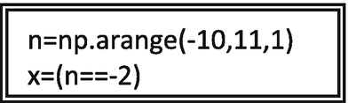
• 2. The value of the signal ‘x’ shown in the following python code is high at n =?

  

  • A. −1

  • B. −2

  • C. 0

  • D. 2

• 3. If the variable ‘x’ contains the signal of interest, then the variable ‘y’ in the following python code returns

  

  • A. Maximum value of the signal

  • B. Minimum value of the signal

  • C. Energy of the signal

  • D. Power of the signal

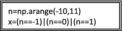
• 4. The signal generated in the variable ‘x’ after executing the following segment of code is

  

  • A. x[n] = δ[n] + δ[n – 1] – δ[n + 1]

  • B. x[n] = δ[n + 1] + δ[n] + δ[n – 1]

  • C. x[n] = δ[n + 1] + δ[n] – δ[n – 1]

  • D. x[n] = δ[n + 1] + 2δ[n] + δ[n – 1]

• 5. The signal generated in the variable ‘x’ after executing the following segment of code is

  

  • A. Unit sample sequence

  • B. Unit step sequence

  • C. Unit ramp sequence

  • D. Real exponential sequence

• 6. What would be the energy of the signal ‘x’ which is stored in variable ‘E’ if the following code segment is executed?

  

  • A. 1J

  • B. 2J

  • C. 3J

  • D. 4J

• 7. What operation is performed on the input signal ‘x’ if the following segment of code is executed?

  

  • A. Convolution of signal ‘x’ with itself

  • B. Correlation of the signal ‘x’ with itself

  • C. Power spectral estimation of the signal ‘x’

  • D. Energy density estimation of signal ‘x’

• 8. A square wave is fed to a lowpass filter, the resulting signal is

  • A. Sine wave

  • B. Cosine wave

  • C. Triangular wave

  • D. Inverted square wave

• 9. The energy of the signal is unaltered by the following mathematical operation

  • A. Downsampling of the signal by a factor of ‘M’

  • B. Upsampling the signal by a factor of ‘L’

  • C. Amplitude scaling

  • D. Folding of the signal

• 10. The energy of the signal is unaltered by the following mathematical operation:

  • A. Downsampling of the signal by a factor of ‘M’

  • B. Upsampling the signal by a factor of ‘L’

  • C. Delaying or advancing the signal by a factor of ‘k’

  • D. Amplitude scaling of the signal

• 11. Upsampling by a factor of ‘L’ inserts

  • A. ‘L’ zeros between successive samples

  • B. ‘L – 1’ zeros between successive samples

  • C. ‘L + 1’ zeros between successive samples

  • D. ‘L + 2’ zeros between successive samples

• 12. If a discrete-time signal x[n] obeys the relation x[−n] = x[n], then the signal is

  • A. Odd signal

  • B. Even signal

  • C. Either even or odd signal

  • D. Neither even nor odd signal

• 13. Sum of elements of finite duration discrete-time odd signal is

  • A. Infinite

  • B. One

  • C. Zero

  • D. Always negative

• 14. The python code shown below generates the following signal in the variable ‘x’

  

  • A. u[n]

  • B. u[−n]

  • C. u[n + 5]

  • D. u[n – 5]

• 15. The product of two odd signal results in

  • A. Odd signal

  • B. Even signal

  • C. Either even or odd signal depending on the length of the signals

  • D. Neither even nor odd signal

• 16. Identify the statement which is FALSE

  • A. Autocorrelation is finding the relative similarity of the signal to itself.

  • B. Autocorrelation is an even function.

  • C. Autocorrelation attains its maximum value at zero lag.

  • D. Auto correlation is an odd function.

• 17. What will be the fundamental period of the signal ‘x’ if the following python code is executed?

  

  • A. 1

  • B. 2

  • C. 3

  • D. 4

• 18. Assertion: Highpass filter act as change detector

  Reason: Highpass filter has the ability to detect the change in the input signal

  • A. Both assertion and reason are true.

  • B. Assertion is true, reason is false.

  • C. Assertion is false, reason may be true.

  • D. Both assertion and reason are false.

• 19. What will be the length of the signal ‘y’ if the following code segment is executed?

  

  • A. 11

  • B. 21

  • C. 31

  • D. 41

• 20. What will be the impulse response (h[n]) if the following code segment is executed?

  

  • A. h[n] = δ[n]

  • B. h[n] = δ[n − 1]

  • C. h[n] = u[n]

  • D. h[n] = u[n − 1]

• 21. Identify the statement that is WRONG with respect to ‘folding’ or ‘time reversal’ operation

  • A. Folding operation does not alter the energy of the signal.

  • B. Folding increases the length of the signal.

  • C. If the folded version of the signal is equal to the signal itself, then the signal is even signal.

  • D. If the folded version of the signal is equal to the signal itself, then the signal is odd signal.

• 22. If x[n] is a unit step signal, then the following signal (y[n]) generated from x[n] is

  

  • A. Unit sample signal

  • B. Unit step signal

  • C. Unit ramp signal

  • D. Real exponential signal

• 23. The fundamental frequency of the signal generated by executing the following code is

  

  • A. ω = π/2 rad/sample

  • B. ω = π rad/sample

  • C. ω = π/4 rad/sample

  • D. ω = π/8 rad/sample

Bibliography

Lonnie C. Ludeman, “Fundamentals of Digital Signal Processing”, John Wiley and Sons, 1986.
S. Esakkirajan, T. Veerakumar and Badri N Subudhi, “Digital Signal Processing”, McGraw Hill, 2021.
Sophocles Orfanidis, “Introduction to Signal Processing”, Pearson, 1995.
Hwei P. Hsu, “Signals and Systems”, Schaum’s outline series, McGraw Hill Education, 2017.
Maurice Charbit, “Digital Signal Processing with Python Programming”, Wiley-ISTE, 2017.
Author information
Authors and Affiliations
Rights and permissions
Copyright information
© 2024 The Author(s), under exclusive license to Springer Nature Singapore Pte Ltd.
About this chapter
Cite this chapter
Esakkirajan, S., Veerakumar, T., N. Subudhi, B. (2024). Generation and Operation on Discrete-Time Sequence. In: Digital Signal Processing. Springer, Singapore. https://doi.org/10.1007/978-981-99-6752-0_3
Download citation
DOI: https://doi.org/10.1007/978-981-99-6752-0_3
Published:
Publisher Name: Springer, Singapore
Print ISBN: 978-981-99-6751-3
Online ISBN: 978-981-99-6752-0
eBook Packages: Computer ScienceComputer Science (R0)