On MAX–SAT with Cardinality Constraint

Abstract

We consider the weighted MAX–SAT problem with an additional constraint that at most k variables can be set to true. We call this problem k –WMAX–SAT. This problem admits a $(1 - \frac{1}{e})$-factor approximation algorithm in polynomial time [Sviridenko, Algorithmica 2001] and it is proved that there is no $(1-\frac{1}{e} + \epsilon )$-factor approximation algorithm in $f(k)\cdot n^{o(k)}$ time for Maximum Coverage, the unweighted monotone version of k –WMAX–SAT [Manurangsi, SODA 2020]. Therefore, we study two restricted versions of the problem in the realm of parameterized complexity.

• 1. When the input is an unweighted 2–CNF formula (the problem is called k –MAX–2SAT), we design an efficient polynomial-size approximate kernelization scheme. That is, we design a polynomial-time algorithm that given a 2–CNF formula $\psi$ and $\epsilon >0$, compresses the input instance to a 2–CNF formula $\psi ^{\star }$ such that any c-approximate solution of $\psi ^{\star }$ can be converted to a $c(1-\epsilon )$-approximate solution of $\psi$ in polynomial time.

• 2. When the input is a planar CNF formula, i.e., the variable-clause incident graph is a planar graph, we show the following results:

  • There is an FPT algorithm for k –WMAX–SAT on planar CNF formulas that runs in $2^{O(k)}\cdot (C+V)$ time.

  • There is a polynomial-time approximation scheme for k –WMAX–SAT on planar CNF formulas that runs in time $2^{O(\frac{1}{\epsilon })}\cdot k\cdot (C+V)$.

  The above-mentioned C and V are the number of clauses and variables of the input formula respectively.

1 Introduction

In this paper, we study the well-studied MAX–SAT problem with cardinality constraint. The weighted version of the problem is formally defined as follows.

k –MAX–SAT and its monotone version (a version in which negated literals are not allowed) Maximum Coverage are well studied both in the realm of approximation algorithms and parameterized complexity. The input of Maximum Coverage is a family $\mathcal{F}$ of subsets of a universe U and a positive integer k. The goal is to find $S_1, S_2, \dots , S_k \in \mathcal{F}$ that maximizes $|S_1 \cup S_2 \cup \dots \cup S_k|$.

Maximum Coverage, and hence k –MAX–SAT are known to be NP-complete and W[2]-hard because Maximum Coverage is a more general case of the Dominating Set problem. A simple greedy approximation algorithm for Maximum Coverage outputs a $(1-\frac{1}{e})$-approximate solution, where e is the base of the natural logarithm. This greedy approximation algorithm is essentially optimal for Maximum Coverage [7]. Sviridenko [18] obtained a $(1-\frac{1}{e})$-factor approximation in polynomial time for k –WMAX–SAT. Recently, Manurangsi [14] showed that there is no $f(k) \cdot n^{o(k)}$ time algorithm that can approximate Maximum Coverage within a factor of $(1-\frac{1}{e}+\epsilon )$ for any $\epsilon >0$ and any function f, assuming Gap Exponential Time Hypothesis (Gap-ETH). Thus, to obtain tractable results for k –WMAX–SAT in the realm of parameterized complexity and approximation algorithms, we need to restrict the input to different classes of formulas. We study cardinality constrained unweighted MAX–SAT when the number of literals in each clause is at most 2. This problem is called k –MAX–2SAT. The problem is formally defined below.

k –MAX–2SAT and its monotone version Max– k –Vertex Cover (shortly Max k –VC) are extensively studied [3, 9, 10, 13, 16, 17]. The best-known polynomial-time approximation ratio for k –MAX–2SAT is 0.75 [9]. Raghavendra and Tan [17] designed an $\alpha$-approximation algorithm for some $\alpha > 0.92$ that runs in time $n^{\textsf{poly}(n/k)}$, where n is the number of variables in the input formula [13]. That is, this algorithm runs in polynomial time when k is a constant fraction of V. Assuming Unique Games Conjecture (UGC), it is NP-hard to approximate k –MAX–2SAT with a factor better than 0.929 [1].

The monotone variant of the problem, Max k –VC gives an interesting connection between approximate kernelization and approximation algorithms. Here, given a graph G, our objective is to find a vertex subset S of size k such that the number of edges in G with at least one endpoint in S is maximized. Max k –VC is W[1]-hard and Marx [15] designed the first FPT approximation scheme for the problem, where k is the parameter. Lokshtanov et al. [12] showed that, indeed the steps of the algorithm by Marx can be converted to get an efficient polynomial-size approximate kernelization scheme (EPSAKS). We refer to Sect. 2 for the definition of approximate kernelization. Manurangsi [13] improved the kernel size to $O(k/\epsilon )$ and the running time of FPT approximation scheme to $(1/\epsilon )^{O(k)}n^{O(1)}$ for Max k -VC. Manurangsi applied the algorithm of Raghavendra and Tan [17] for k –MAX–2SAT on the linear size approximate kernel to obtain an approximation factor of 0.92 for Max k –VC. Approximating Max k –VC with a factor better than 0.929 is also NP-hard assuming UGC [1]. We prove that k –MAX–2SAT admits an EPSAKS.

Theorem 1

Given a set of t clauses $\mathcal {C}_{\mathcal {F}} = \{C_1, C_2, \dots , C_t\}$ of a 2–CNF formula $\mathcal {F}$ and a positive integer k, there is an EPSAKS (efficient polynomial-size approximate kernelization scheme) for k –MAX–2SAT such that the size of the output of the reduction algorithm is upper-bounded by $O\left( \frac{k^5}{\epsilon ^2}\right)$.

We also study k –WMAX–SAT when the input is a planar CNF formula, that is, the variable-clause incident graph is a planar graph. Restricting MAX–SAT to planar formulas has been already considered in the realm of approximation algorithms [4, 11]. We prove the following result for k –WMAX–SAT on planar CNF formulas.

Theorem 2

Given a set of t clauses $\mathcal {C}_{\mathcal {F}} = \{C_1, C_2, \dots , C_t\}$ of a planar CNF formula $\mathcal {F}$, a weight function $w: \mathcal {C}_{\mathcal {F}} \rightarrow \mathbb {R}^+$ and a positive integer k, there is an FPT algorithm for k –WMAX–SAT that runs in $O(2^{36k} \cdot k^3\cdot |\mathcal {C}_{\mathcal {F}} \cup V_{\mathcal {F}}|)$ time.

Khanna and Motwani [11] already designed a PTAS for k –MAX–SAT (the unweighted version) on planar formulas. Using a similar technique, we show that the weighted version k –WMAX–SAT also admits a PTAS.

Theorem 3

Given a set of t clauses $\mathcal {C}_{\mathcal {F}} = \{C_1, C_2, \dots , C_t\}$ of a planar CNF formula $\mathcal {F}$, a weight function $w: \mathcal {C}_{\mathcal {F}} \rightarrow \mathbb {R}^+$ and a positive integer k, there is a polynomial-time approximation scheme that runs in $O(\frac{1}{\epsilon ^2}\cdot 2^{\frac{36}{\epsilon }} \cdot k\cdot |\mathcal {C}_{\mathcal {F}} \cup V_{\mathcal {F}}|)$ time and finds $S \subseteq V_{\mathcal {F}}$ such that $|S| \le k$ and

$$k\text {--WMAX--SAT}(\mathcal {C}_\mathcal {F}, w, k, S) \ge (1-\epsilon ) \cdot \text {OPT}(\mathcal {C}_\mathcal {F}, w, k)$$

Here, $\text {OPT}(\mathcal {C}_\mathcal {F}, w, k)$ is the maximum total weight of clauses in $\mathcal {C}_\mathcal {F}$ that can be satisfied by an assignment where at most k variables are set to true.

2 Preliminaries

Definition 1 (Conjunctive Normal Form (CNF))

A formula is said to be in Conjunctive Normal Form (CNF) if it looks like $C_1 \wedge C_2 \wedge \dots \wedge C_t$ where each $C_i = (l_1 \vee l_2 \vee \dots \vee l_{t_i})$ is called a clause and each $l_i$ is called a literal. A literal is either a variable, called positive literal, or the negation of a variable, called negative literal.

A formula is said to be in 2–Conjunctive Normal Form (2–CNF) if it is in CNF and all of its clauses contain 2 literals.

We assume, without loss of generality, that for each variable v, at most one of the v and $\lnot v$ is contained in a clause, no literal is repeated in a clause and all clauses are distinct.

For a CNF formula $\mathcal {F}$, the set of clauses and the set of variables appeared in $\mathcal {F}$ are denoted by $\mathcal {C}_{\mathcal {F}} = \{C_1, C_2, \dots , C_t\}$ and $V_{\mathcal {F}} = \{v_1, v_2, \dots , v_n\}$, respectively.

2.1 Parameterized Complexity

For a parameterized maximization problem $\varPi$ and a solution s to the instance (I, k) of $\varPi$, we denote the value of s by $\varPi (I, k, s)$, and the task is to find a solution with the maximum possible value. We state the following definitions slightly modified from the Kernelization book [8].

Definition 2 (FPT optimization problem)

A parameterized optimization problem $\varPi$ is fixed-parameter tractable (FPT) if there is an algorithm (called FPT algorithm) that solves $\varPi$, such that the running time of the algorithm on instances of size n with parameter k is upper-bounded by $f(k)\cdot n^{O(1)}$ for a computable function f.

Definition 3

($\alpha$-approximate polynomial-time preprocessing algorithm). Let $0 < \alpha \le 1$ be a real number and $\varPi$ be a parameterized maximization problem. An $\alpha$-approximate polynomial-time preprocessing algorithm $\mathcal {A}$ for $\varPi$ is a pair of polynomial-time algorithms. The first one is called the reduction algorithm $\mathcal {R}_\mathcal {A}$, and given an instance (I, k) of $\varPi$, it outputs another instance $(I', k') = \mathcal {R}_\mathcal {A}(I, k)$. The second algorithm is called the solution lifting algorithm. This algorithm takes an instance (I, k) of $\varPi$, the output instance $(I', k')$ of the reduction algorithm, and a solution $s'$ to the instance $(I', k')$. The solution lifting algorithm works in time polynomial in $|I|,k,|I'|, k'$ and $|s'|$, and outputs a solution s to (I, k) such that

$$\frac{\varPi (I, k, s)}{OPT(I, k)} \ge \alpha \cdot \frac{\varPi (I', k', s')}{OPT(I', k')}$$

Definition 4

($\alpha$-approximate kernelization). An $\alpha$-approximate kernelization ($\alpha$-approximate kernel) is an $\alpha$-approximate polynomial-time preprocessing algorithm $\mathcal {A}$ such that $\text {size}_\mathcal {A}$ is upper-bounded by a computable function $g: \mathbb {N} \rightarrow \mathbb {N}$ where $\text {size}_\mathcal {A}$ is defined as follows:

$$\begin{aligned} \text {size}_\mathcal {A}(k) &= \sup \{|I'| + k': (I', k')\\ &= \mathcal {R}_\mathcal {A}(I, k)\ \text {for any instance }(I, k) \text {of the problem}\} \end{aligned}$$

If the upper-bound $g(\cdot )$ is a polynomial function of k, we say $\mathcal {A}$ is an $\alpha$-approximate polynomial kernel.

Definition 5 (polynomial-size approximate kernelization scheme (PSAKS))

  A polynomial-size approximate kernelization scheme (PSAKS) for a parameterized maximization problem $\varPi$, is a family of $(1 - \epsilon )$-approximate polynomial kernels for every $0 < \epsilon < 1$.

Definition 6 (Efficient PSAKS)

An efficient PSAKS (EPSAKS) is a PSAKS such that for every $(1 - \epsilon )$-approximate polynomial kernel $\mathcal {A}$ in that, $size_{\mathcal {A}}(k)$ is upper-bounded by $f(\frac{1}{\epsilon })\cdot k^c$ for a function f and a constant c independent of I, k and $\epsilon$.

2.2 Tree Decomposition and Tree-Width

We state the following definitions and lemmas from the Parameterized Algorithms book [5].

Definition 7 (Tree decomposition)

A tree decomposition of a graph G is a pair $\mathcal {T} =(T, \{X_t\}_{t\in V(T)})$, where T is a tree whose every node t is assigned a vertex subset $X_t \subseteq V(G)$, called a bag, such that the following three conditions hold:

• Vertex coverage: $\bigcup _{t\in V(T)} X_t = V(G)$, i.e., every vertex of G is in at least one bag.

• Edge coverage: For every $uv\in E(G)$, there exists a node t of T such that bag $X_t$ contains both u and v.

• Coherence: For every $u\in V(G)$, the set $T_u = \{t \in V(T) : u\in X_t\}$, i.e., the set of nodes whose corresponding bags contain u, induces a connected subtree of T.

The width of tree decomposition $\mathcal {T} =(T, \{X_t\}_{t\in V(T)})$ equals $\max _{t\in V(T)}|X_t|-1$.

Definition 8 (Tree-width)

The tree-width of a graph G is the minimum possible width of a tree decomposition of G.

Definition 9 (Nice tree decomposition)

A tree decomposition $\mathcal {T} =(T, \{X_t\}_{t\in V(T)})$, rooted from $r \in V(T)$, is called nice if the following conditions are satisfied:

• $X_r = \emptyset$ and $X_l = \emptyset$ for every leaf l of T.

• Every non-leaf node of T is of one of the following three types:

  • Introduce node: a node t with exactly one child $t'$ such that $X_t = X_{t'} \cup \{v\}$ for some vertex $v \notin X_{t'}$. We say that v is introduced at t.

  • Forget node: a node t with exactly one child $t'$ such that $X_t = X_{t'} \setminus \{w\}$ for some vertex $w \in X_{t'}$. We say that w is forgotten at t.

  • Join node: a node t with two children $t_1, t_2$ such that $X_t = X_{t_1} = X_{t_2}$.

Lemma 1

If a graph G admits a tree decomposition of width at most d, then it also admits a nice tree decomposition of width at most d. Moreover, given a tree decomposition $\mathcal {T} =(T, \{X_t\}_{t\in V(T)})$ of G of width at most d, one can in time $O(d^2 \cdot \max (|V(T)|, |V(G)|))$ compute a nice tree decomposition of G of width at most d that has $O(d\cdot |V(G)|)$ nodes.

3 EPSAKS for k–MAX–2SAT with Cardinality Constraint

In this section, we show that k –MAX–2SAT admits an EPSAKS. That is we prove Theorem 1.

There are two main observations used in the algorithm. First, since one can satisfy all clauses containing at least one negative literal by setting all the variables to false, the optimal value is not less than the number of clauses containing negative literals. Second, if a variable v appears positively in many clauses, then one can satisfy all those clauses by setting v true and all the other variables false.

Let $\mathcal {F}$ be a 2–CNF formula with clause set $\mathcal {C}_{\mathcal {F}}$ and variable set $V_{\mathcal {F}}$. For a variable $v \in V_{\mathcal {F}}$, we denote the number of clauses in the form of $(v \vee u)$, $(v \vee \lnot u)$, $(\lnot v \vee u)$ and $(\lnot v \vee \lnot u)$ by $d_+^+(v)$, $d_+^-(v)$, $d_-^+(v)$ and $d_-^-(v)$ respectively. For $V \subseteq V_{\mathcal {F}}$ we denote the set of negation of variables in V with $\lnot V$, i.e., $\lnot V = \{\lnot s ~|~ s \in V\}$. Let $P_{\mathcal {F}} = \{p_1, p_2, \dots , p_{l}\}$ be the set of variables that appear only in clauses containing two positive literals, i.e., in the form of $(v \vee u)$, and $N_{\mathcal {F}} = V_{\mathcal {F}} \setminus P_{\mathcal {F}}$. We suppose, without loss of generality, $d_+^+(p_1) \ge d_+^+(p_2) \ge \dots \ge d_+^+(p_{l})$.

We now describe a $(1 - \epsilon )$-approximate polynomial-time preprocessing algorithm $\mathcal {A_{\epsilon }}$ for an arbitrary $\epsilon$.

Reduction Algorithm$\mathcal {R}_{\epsilon }$: $\mathcal {R}_{\epsilon }$ takes the set of clauses $\mathcal {C}_{\mathcal {F}} = \{C_1, C_2, \dots , C_t\}$ of a 2–CNF formula $\mathcal {F}$ and a parameter k as input. Set $\lambda$ to be equal to $\frac{4\cdot {k \atopwithdelims ()2}}{\epsilon }$. Recall that $P_{\mathcal {F}} = \{p_1, p_2, \dots , p_{l}\}$ is the set of variables that appear only in clauses containing two positive literals. Let $\tilde{P}_{\mathcal {F}} = \{p_1, p_2, \dots , p_{\tilde{l}}\}$ where $\tilde{l} = \min (l, {k+k\lambda })$ and $\tilde{\mathcal {C}}_{\mathcal {F}} \subseteq \mathcal {C}_{\mathcal {F}}$ be the set of clauses whose both variables are in $P_{\mathcal {F}} \setminus \tilde{P}_{\mathcal {F}}$. If both of the following requirements are satisfied, $\mathcal {R}_{\epsilon }$ outputs $(\mathcal {C}_{\mathcal {F}} \setminus \tilde{\mathcal {C}}_{\mathcal {F}}, k)$, otherwise it outputs $(\{C_1\}, k + 1)$.

• (R1) There are $< \lambda$ clauses with at least one negative literal.

• (R2) $d_+^+(v) < \lambda$ for every variable $v \in V_{\mathcal {F}}$.

Solution Lifting Algorithm $\mathcal {L}_{\epsilon }$: The algorithm takes $(\mathcal {C}_{\mathcal {F}}, k)$, the output of the reduction algorithm $(\mathcal {C}'_{\mathcal {F}'}, k')$ and a set $S'$ of at most $k'$ variables appeared in $\mathcal {F}'$. If $k' = k$, $\mathcal {L}_{\epsilon }$ outputs $S = S'$. Otherwise, let $V_{\mathcal {F}} = \{v_1, v_2, \dots , v_n\}$ and without loss of generality suppose

$$d_+^+(v_1) - d_-^+(v_1) \ge d_+^+(v_2) - d_-^+(v_2) \ge \dots \ge d_+^+(v_n) - d_-^+(v_n)$$

Then the algorithm outputs

$$S = \{v\in \{v_1, v_2, \dots , v_k\}~|~ d_+^+(v) - d_-^+(v) > 0\}$$

We next show that $\mathcal {A}_{\epsilon }$ is a $(1 - \epsilon )$-approximate polynomial-time preprocessing algorithm. To do so, we need to prove the following lemmas.

Lemma 2

Suppose $d_+^+(v) < \lambda$ for every $v \in V_{\mathcal {F}}$. Let $S^*$ be an optimal solution for $(\mathcal {C}_{\mathcal {F}}, k)$ such that $S^* \cap P_{\mathcal {F}}$ is lexicographically smallest with respect to $p_1, p_2, \dots , p_{l}$. Then $(S^* \cap P_{\mathcal {F}}) \subseteq \tilde{P}_{\mathcal {F}} = \{p_1, p_2, \dots , p_{\tilde{l}}\}$.

Proof

If $\tilde{l} = l$, we have $\tilde{P}_{\mathcal {F}} = P_{\mathcal {F}}$. So $(S^* \cap P_{\mathcal {F}}) \subseteq P_{\mathcal {F}}=\tilde{P}_{\mathcal {F}}$ and we are done.

So suppose $\tilde{l} = k+k\lambda$ and for the sake of contradiction, suppose there is $p \in (S^* \cap P_{\mathcal {F}})$ such that $p \notin \tilde{P}_{\mathcal {F}}$. Define the set A as the following:

$$\begin{aligned} A = S^* \cup \left\{ v \in V_{\mathcal {F}} ~|~ \exists (v \vee u) \in \mathcal {C}_{\mathcal {F}}: u \in S^* \right\} \end{aligned}$$

Since $|S^*| \le k$ and $\forall v \in V_{\mathcal {F}} : d_+^+(v) < \lambda$, we have $|A| < k + k \lambda$. Therefore, there is a variable $q \in \{p_1, p_2, \dots , p_{k+k\lambda }\}$ which is not in A, i.e., $q \in \tilde{P}_{\mathcal {F}} \setminus A$.

Note that since $p, q \in P_{\mathcal {F}}$, p and q appear only in clauses with two positive literals, So we have

Therefore, $S^* \setminus \{p\} \cup \{q\}$ is an optimal solution and since $p \notin \tilde{P}_{\mathcal {F}}$ but $q \in \tilde{P}_{\mathcal {F}}$, $(S^* \setminus \{p\} \cup \{q\}) \cap P_{\mathcal {F}}$ is lexicographically smaller than $S^* \cap P_{\mathcal {F}}$, which implies a contradiction.

Lemma 3

If $d_+^+(v) < \lambda$ for every $v \in V_{\mathcal {F}}$, then $\text {OPT}(\mathcal {C}_{\mathcal {F}}, k) = \text {OPT}(\mathcal {C}_{\mathcal {F}} \setminus \tilde{\mathcal {C}}_{\mathcal {F}}, k)$.

Proof

Since $(\mathcal {C}_{\mathcal {F}} \setminus \tilde{\mathcal {C}}_{\mathcal {F}}) \subseteq \mathcal {C}_{\mathcal {F}}$, we have $\text {OPT}(\mathcal {C}_{\mathcal {F}}, k) \ge \text {OPT}(\mathcal {C}_{\mathcal {F}} \setminus \tilde{\mathcal {C}}_{\mathcal {F}}, k)$. For the other direction, let $S^*$ be the optimal solution of $(\mathcal {C}_{\mathcal {F}}, k)$ described in the Lemma 2. By Lemma 2 we know $S^* \cap (P_{\mathcal {F}} \setminus \tilde{P}_{\mathcal {F}}) = \emptyset$ and therefore, by setting only variables of $S^*$ true, none of the clauses with both literals from $P_{\mathcal {F}} \setminus \tilde{P}_{\mathcal {F}}$, i.e., clauses in $\tilde{\mathcal {C}}_{\mathcal {F}}$, gets satisfied. This implies

$$\underbrace{k\text {--MAX--2SAT}(\mathcal {C}_{\mathcal {F}}, k, S^*)}_{=\text {OPT}(\mathcal {C}_{\mathcal {F}}, k)}= \underbrace{k\text {--MAX--2SAT}(\mathcal {C}_{\mathcal {F}} \setminus \tilde{\mathcal {C}}_{\mathcal {F}}, k, S^*)}_{\le \text {OPT}(\mathcal {C}_{\mathcal {F}} \setminus \tilde{\mathcal {C}}_{\mathcal {F}}, k)}$$

which proves the lemma.

Lemma 4

$\mathcal {A}_{\epsilon }$ is a $(1 - \epsilon )$-approximate polynomial-time preprocessing algorithm.

Proof

Clearly, both $\mathcal {R}_{\epsilon }$ and $\mathcal {L}_{\epsilon }$ are polynomial algorithms. In the solution lifting algorithm, note that $\mathcal {C}'_{\mathcal {F}'} \subseteq \mathcal {C}_{\mathcal {F}}$ and thus $S' \subseteq V_{\mathcal {F}}$. This implies that the output of $\mathcal {L}_{\epsilon }$ is a subset of $V_{\mathcal {F}}$ with size $\le k$ and therefore a solution to instance $(\mathcal {C}_{\mathcal {F}}, k)$ of k –MAX–2SAT.

We now show that

$$\frac{k\text {--MAX--2SAT}(\mathcal {C}_{\mathcal {F}}, k, S)}{\text {OPT}(\mathcal {C}_{\mathcal {F}}, k)} \ge (1 - \epsilon ) \cdot \frac{k\text {--MAX--2SAT}(\mathcal {C}'_{\mathcal {F}'}, k', S')}{\text {OPT}(\mathcal {C}'_{\mathcal {F}'}, k')}$$

We consider two cases:

• 1. The aforementioned requirements, (R1) and (R2) are satisfied. In this case, $\mathcal {R}_{\epsilon }$ outputs $(\mathcal {C}'_{\mathcal {F}'}, k') = (\mathcal {C}_{\mathcal {F}} \setminus \tilde{\mathcal {C}}_{\mathcal {F}}, k)$ and since $k = k'$, $\mathcal {L}_{\epsilon }$ would output $S = S'$. Since $\mathcal {C}_{\mathcal {F}} \setminus \tilde{\mathcal {C}}_{\mathcal {F}} \subseteq \mathcal {C}_{\mathcal {F}}$, we have

  $$ k \text {--MAX--2SAT}(\mathcal {C}_{\mathcal {F}}, k, S') \ge k\text {--MAX--2SAT}(\mathcal {C}_{\mathcal {F}}\setminus \tilde{\mathcal {C}}_{\mathcal {F}}, k, S')$$

  And by Lemma 3 we get

  $$\begin{aligned} \frac{k \text {--MAX--2SAT}(\mathcal {C}_{\mathcal {F}}, k, S')}{\text {OPT}(\mathcal {C}_{\mathcal {F}}, k)} &\ge \frac{k\text {--MAX--2SAT}(\mathcal {C}_{\mathcal {F}}\setminus \tilde{\mathcal {C}}_{\mathcal {F}}, k, S')}{\text {OPT}(\mathcal {C}_{\mathcal {F}}\setminus \tilde{\mathcal {C}}_{\mathcal {F}}, k)} \\ {} &\ge (1 - \epsilon ) \cdot \frac{k \text {--MAX--2SAT}(\mathcal {C}_{\mathcal {F}}\setminus \tilde{\mathcal {C}}_{\mathcal {F}}, k, S')}{\text {OPT}(\mathcal {C}_{\mathcal {F}}\setminus \tilde{\mathcal {C}}_{\mathcal {F}}, k)} \end{aligned}$$

  Which completes the proof for the first case.

• 2. At least one of the requirements, (R1) and (R2) is not satisfied. If (R1) is not satisfied we have $k\text {--MAX--2SAT}(\mathcal {C}_{\mathcal {F}}, k, \emptyset ) \ge \lambda$. If (R2) is not satisfied, there is a variable $v \in V_{\mathcal {F}}$ such that $d_+^+(v) \ge \lambda$, thus $k\text {--MAX--2SAT}(\mathcal {C}_{\mathcal {F}}, k, \{v\}) \ge \lambda$. Therefore, in this case $\text {OPT}(\mathcal {C}_{\mathcal {F}}, k) \ge \lambda$. Note that for any solution S:

  $$\begin{aligned} k \text {--MAX--2SAT}(\mathcal {C}_{\mathcal {F}}, k, S) &= \sum _{v \in V_{\mathcal {F}}} d_-^+(v) - \left| \{(\lnot v \vee u) ~|~ v \in S, u \in V_{\mathcal {F}} \setminus S\}\right| \nonumber \\ &+ \frac{\sum _{v \in V_{\mathcal {F}}} d_-^-(v)}{2} - \left| \{(\lnot v \vee \lnot u) ~|~ v, u \in S\}\right| \nonumber \\ &+ \sum _{v \in S} d_+^+(v) - \left| \{(v \vee u) ~|~ v, u \in S\}\right| \end{aligned}$$

  And also:

  $$\begin{aligned} & \left| \{(\lnot v \vee u) ~|~ v \in S, u \in V_{\mathcal {F}} \setminus S\}\right| = \left( \sum _{v \in S} d_-^+(v) - \left| \{(\lnot v \vee u) ~|~ v, u \in S\}\right| \right) \end{aligned}$$

  Which implies:

  $$\begin{aligned} k \text {--MAX--2SAT}(\mathcal {C}_{\mathcal {F}}, k, S) &= \sum _{v \in V_{\mathcal {F}}} d_-^+(v) - \left( \sum _{v \in S} d_-^+(v) - \left| \{(\lnot v \vee u) ~|~ v, u \in S\}\right| \right) \nonumber \\ &+ \frac{\sum _{v \in V_{\mathcal {F}}} d_-^-(v)}{2} - \left| \{(\lnot v \vee \lnot u) ~|~ v, u \in S\}\right| \nonumber \\ &+ \sum _{v \in S} d_+^+(v) - \left| \{(v \vee u) ~|~ v, u \in S\}\right| \end{aligned}$$

  (1)

  And since $|S| \le k$ and all clauses are distinct, we have:

  $$\begin{aligned} \left| \{(\lnot v \vee \lnot u) | v, u \in S\}\right| \quad , \quad \left| \{(v \vee u) | v, u \in S\}\right| \nonumber \nonumber &\quad \le \quad {k \atopwithdelims ()2} \end{aligned}$$

  Therefore, considering Eq. (1) we have:

  $$\begin{aligned} k \text {--MAX--2SAT}(\mathcal {C}_{\mathcal {F}}, k, S) \nonumber \ge &\sum _{v \in V_{\mathcal {F}}} d_-^+(v) - \left( \sum _{v \in S} d_-^+(v) - \left| \{(\lnot v \vee u) ~|~ v, u \in S\}\right| \right) \\ +&\frac{\sum _{v \in V_{\mathcal {F}}} d_-^-(v)}{2} - {k \atopwithdelims ()2} +\sum _{v \in S} d_+^+(v) - {k \atopwithdelims ()2}\nonumber \\ =&\sum _{v \in V_{\mathcal {F}}} d_-^+(v) + \left| \{(\lnot v \vee u) ~|~ v, u \in S\}\right| \nonumber \\ &+\frac{\sum _{v \in V_{\mathcal {F}}} d_-^-(v)}{2} + \left( \sum _{v \in S} d_+^+(v) - \sum _{v \in S} d_-^+(v)\right) - 2 \cdot {k \atopwithdelims ()2} \end{aligned}$$

  (2)

  Note that in this case $\mathcal {R}_{\epsilon }$ outputs $(\mathcal {C}'_{\mathcal {F}'}, k') = (\{C_1\}, k + 1)$ and since $k \ne k'$, $\mathcal {L}_{\epsilon }$ outputs $S = \{v\in \{v_1, v_2, \dots , v_k\}| d_+^+(v) - d_-^+(v) > 0\}$. Let $S^*\subseteq V_{\mathcal {F}}$ be an optimal solution to $(\mathcal {C}_{\mathcal {F}}, k)$. Then we have:

  $$\begin{aligned} \sum _{v \in S} d_+^+(v) - d_-^+(v) \ge \sum _{v \in S^*} d_+^+(v) - d_-^+(v) \end{aligned}$$

  And considering inequality (2):

  

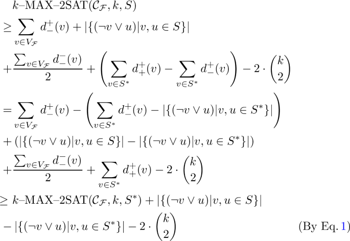
  Plugging $\left| \{(\lnot v \vee u) | v, u \in S^*\}\right| \le 2\cdot {k \atopwithdelims ()2}$ into the above inequality, we get:

  

  Finally, as OPT$(\mathcal {C}_{\mathcal {F}}, k) \ge \lambda$ we have:

  $$\begin{aligned} k\text {--MAX--2SAT}(\mathcal {C}_{\mathcal {F}}, k, S) \ge (1 - \epsilon )\cdot \text {OPT}(\mathcal {C}_{\mathcal {F}}, k) \end{aligned}$$

  Which implies $\frac{k\text {--MAX--2SAT}(\mathcal {C}_{\mathcal {F}}, k, S) }{\text {OPT}(\mathcal {C}_{\mathcal {F}}, k)} \ge (1 - \epsilon ) \ge (1 - \epsilon ) \cdot \frac{\text {MAX--2SAT}(\mathcal {C}'_{\mathcal {F}'}, k', S')}{\text {OPT}(\mathcal {C}'_{\mathcal {F}'}, k')}$ and proves the second case.

The next lemma states an upper-bound for $\text {size}_{\mathcal {A}_{\epsilon }}(k)$.

Lemma 5

$\text {size}_{\mathcal {A}_{\epsilon }}(k)$ is of $O\left( \frac{k^5}{\epsilon ^2}\right)$ where $\text {size}_{\mathcal {A}_{\epsilon }}(k)$ is defined in Definition 4.

Proof

Note that $\mathcal {R}_{\epsilon }$ returns either $(\{C_1\}, k + 1)$ or $(\mathcal {C}_{\mathcal {F}} \setminus \tilde{\mathcal {C}}_{\mathcal {F}}, k)$. In the first case $\text {size}_{\mathcal {A}_{\epsilon }}(k)$ is of O(1) and so we need to only consider the case of returning $(\mathcal {C}_{\mathcal {F}} \setminus \tilde{\mathcal {C}}_{\mathcal {F}}, k)$. In this case, (R1) and (R2) are satisfied. Since (R1) is satisfied, there are less than $2\lambda$ variables that appear in at least one clause with at least one negative literal, i.e., $|N_{\mathcal {F}}| < 2 \lambda$. Therefore, $|N_{\mathcal {F}} \cup \tilde{P}_{\mathcal {F}}| \le 2\lambda +\tilde{l} \le 2\lambda + k\lambda + k = O(k\lambda )$. (R1) and (R2) together imply that $d_+^+(v) + d_+^-(v) + d_-^+(v) + d_-^-(v) < d_+^+(v) + \lambda < 2\lambda$ which means every variable $v\in V_{\mathcal {F}}$ appears in less than $2\lambda$ clauses of $\mathcal {F}$. Therefore, $|\mathcal {C}_{\mathcal {F}} \setminus \tilde{\mathcal {C}}_{\mathcal {F}}|$ is less than $2\lambda \cdot |N_{\mathcal {F}} \cup \tilde{P}_{\mathcal {F}}| = O(k\lambda ^2) = O\left( \frac{k^5}{\epsilon ^2}\right)$.

We finally prove Theorem 1. For convenience, we restate the theorem here.

Theorem 1

Given a set of t clauses $\mathcal {C}_{\mathcal {F}} = \{C_1, C_2, \dots , C_t\}$ of a 2–CNF formula $\mathcal {F}$ and a positive integer k, there is an EPSAKS (efficient polynomial-size approximate kernelization scheme) for k –MAX–2SAT such that the size of the output of the reduction algorithm is upper-bounded by $O\left( \frac{k^5}{\epsilon ^2}\right)$.

Proof

According to Definition 6, the proof is directly derived from Lemma 4 and Lemma 5.

4 k–WMAX–SAT with Cardinality Constraint on Planar Formulas

In this section, we present an FPT algorithm as well as a PTAS (Polynomial-time approximation scheme) for k–WMAX–SAT on a special family of sparse CNF formulas that we will refer to as planar formulas. We now describe this family of formulas.

For a CNF formula $\mathcal {F}$, let $G_\mathcal {F} = (\mathcal {C}_{\mathcal {F}} \cup V_{\mathcal {F}}, E_- \cup E_+)$ be a bipartite graph such that $(C_i, v_j) \in E_+$ if $C_i$ contains $v_j$ and $(C_i, v_j) \in E_-$ if $C_i$ contains $\lnot v_j$. We call $\mathcal {F}$ a planar CNF formula if $G_\mathcal {F}$ is a planar graph.

Both algorithms presented in this section are designed using Baker’s technique [2] and dynamic programming on tree decomposition. First, we need the following lemmas.

Lemma 6

(Eppstein [6]). Let planar graph G have diameter d. Then G has tree-width at most $3d -2$, and a tree-decomposition of G with such a width can be found in time $O(d\cdot |V(G)|)$.

Lemma 7

Let $\mathcal {F}$ be a planar CNF formula. Then there is an algorithm with running time $O(2^{3d} \cdot kd\cdot |\mathcal {C}_{\mathcal {F}} \cup V_{\mathcal {F}}|)$ that takes $\mathcal {C}_\mathcal {F} = \{C_1, C_2, \dots , C_t\}$, a weight function $w: \mathcal {C}_{\mathcal {F}} \rightarrow \mathbb {R}^+$, a positive integer k, and a tree decomposition of $G_\mathcal {F}$ of width at most d with $O(d\cdot |V(G_\mathcal {F})|)$ nodes as input and solves k –WMAX–SAT, i.e., finds $S \subseteq V_{\mathcal {F}}$ such that $|S| \le k$ and setting variables of S to true and other variables to false maximizes the weight of the satisfied clauses.

Proof

First, we construct a nice tree decomposition $\mathcal {T} =(T, \{X_t\}_{t\in V(T)})$ of width at most d with $O(d \cdot |V(G_\mathcal {F})|)$ nodes in time $O(d^3 \cdot |V(G_\mathcal {F})|)$ using Lemma 1. Then, we use a dynamic programming routine.

For each $t \in V(T)$ let $V_t \subseteq V(G_\mathcal {F}) =\mathcal {C}_{\mathcal {F}} \cup V_{\mathcal {F}}$ be the union of all the bags present in the subtree of T rooted at t, including $X_t$. For each $t \in V(T)$, $S \subseteq (X_t \cap V_{\mathcal {F}})$, $C \subseteq (X_t \cap \mathcal {C}_{\mathcal {F}})$ and $0 \le i \le k$ define the following:

If we manage to compute values of dp, then since $X_r = \emptyset$, where r is the root of T, the answer would be dp$[r, \emptyset , \emptyset , k]$ and we can fill the dp array in a bottom-up manner and in the following way:

• Leaf node: If t is a leaf, $X_t = \emptyset$ and we have dp$[t, \emptyset , \emptyset , i] = 0$ for all $0 \le i \le k$. So in this case, filling each cell of dp takes O(1) time.

• Introduce node: If t is an introduce node with child $t'$ that $X_t = X_{t'} \cup \{v\}$, we consider two cases and fill the entries $\text {dp}[t, S, C, i]$ in the following way.

  • 1. $v \in V_{\mathcal {F}}$, i.e., v is a variable. Then $C' \subseteq C$ might be the set of satisfied clauses of $X_{t'}$, if it satisfies one of the two below conditions:

    • (C1) All clauses in $C \setminus C'$ contain a positive literal of v, i.e., Setting v to true satisfies all clauses in $C \setminus C'$.

    • (C2) All clauses in $C \setminus C'$ contain a negative literal of v, i.e., setting v to false satisfies all clauses in $C \setminus C'$.

    So we can compute $\text {dp}[t, S, C, i]$ as follows

    $$ \left\{ \begin{array}{ll} \max _{C' \text {satisfies (C1)}} \text {dp}[t', S \setminus \{v\}, C', i - 1] + w(C \setminus C') &{} \text {if }v \in S\\ \max _{C' \text {satisfies (C2)}} \text {dp}[t', S, C', i] + w(C \setminus C') &{} \text {if }v \notin S \end{array}\right. $$

    So in this case, filling one cell of dp takes $O(2^d)$ time.

  • 1. $v \in \mathcal {C}_{\mathcal {F}}$, i.e., v is a clause. Note that because of edge coverage and coherence properties, $\text {Var}(v) \cap V_t = \text {Var}(v) \cap X_t$ where $\text {Var}(v)$ is the set of variables present in the clause v, either as a positive or negative literal. So, there are two possibilities:

    • (P1) $v \in C$ and v gets satisfied by setting all variables of S to true, $X_t\setminus S$ to false and ignoring variables of $V_{\mathcal {F}} \setminus X_t$.

    • (P2) $v \notin C$ and v is not satisfied by setting all variables of S to true, $X_t\setminus S$ to false and ignoring variables of $V_{\mathcal {F}} \setminus X_t$.

    Therefore, we have:

    $$ \text {dp}[t, S, C, i]= \left\{ \begin{array}{ll} \text {dp}[t', S, C \setminus \{v\}, i] + w(v) &{} \text {if (P1) is true}\\ \text {dp}[t', S, C, i] &{} \text {if (P2) is true}\\ \text {INVALID} &{} \text {otherwise} \end{array}\right. $$

    So, in this case filling one cell of dp takes O(1) time.

  Overall we can fill dp[t, S, C, i] for an introduce node t in $O(2^d)$ time.

• Forget node: If t is a forget node with child $t'$ that $X_t = X_{t'} \setminus \{w\}$, we again consider two cases:

  • 1. $w \in V_{\mathcal {F}}$, i.e., w is a variable. Note that w is either set to true or false and therefore:

    $$ \text {dp}[t, S, C, i]= \max \left\{ \begin{array}{ll} \text {dp}[t', S, C, i]&{} \text {setting }w \text { to false}\\ \text {dp}[t', S \cup \{w\}, C, i] &{} \text {setting }w\text { to true}\\ \end{array}\right. $$

  • 2. $w \in \mathcal {C}_{\mathcal {F}}$, i.e., w is a clause.

    $$ \text {dp}[t, S, C, i]= \max \left\{ \begin{array}{ll} \text {dp}[t', S, C, i] &{} w\text { does not get satisfied}\\ \text {dp}[t', S, C \cup \{w\}, i] &{} w\text { gets satisfied}\\ \end{array}\right. $$

  Note that in this case filling one cell of dp takes O(1) time.

• Join node: If t is a join node with children $t_1$ and $t_2$ that $X_t = X_{t_1} = X_{t_2}$, we consider all possibilities of $S_1, S_2$ and $C_1, C_2$, and compute the value of $\text {dp}[t, S, C, i]$ by:

  $$\begin{aligned} \max _{S_1 \cup S_2 = S,\ C_1 \cup C_2 = C,\ |S_1| \le j \le i} \left( \begin{array}{ll} \ {} &{}\text {dp}[t_1, S_1, C_1, j]\\ +&{}\text {dp}[t_2, S_2, C_2, i - j + |S_1 \cap S_2|]\\ -&{}w(C_1 \cap C_2) \end{array}\right) \end{aligned}$$

  So in the case of join nodes, we can compute the value of each cell of dp in $O(2^{2d})$, because of $2^d$ possibilities for $S_1 \cup C_1$ and at most $2^d$ possibilities for $S_2 \cup C_2$.

The total number of array’s cells is $O(|V(T)| \cdot 2^d \cdot k)$ and we can fill each cell in time $O(2^{2d})$, since by Lemma 1 $|V(T)| = O(d\cdot |V(G_{\mathcal {F}})|) = O(d \cdot |\mathcal {C}_{\mathcal {F}} \cup V_{\mathcal {F}}|)$ we can fill all the cells in time $O(2^{3d} \cdot kd \cdot |\mathcal {C}_{\mathcal {F}} \cup V_{\mathcal {F}}|)$. Again by Lemma 1, constructing T is done in time $O(d^3 \cdot |\mathcal {C}_{\mathcal {F}} \cup V_{\mathcal {F}}|$ which gives us the overall runtime of $O(2^{3d} \cdot kd \cdot |\mathcal {C}_{\mathcal {F}} \cup V_{\mathcal {F}}|)$.

Finally, using the standard technique of backlinks, i.e., memorizing for every cell of dp how its value was obtained, we can find an optimal solution, i.e., a subset $S \subseteq V_{\mathcal {F}}$ such that $|S| \le k$ and setting its variables to true maximizes the weight of the satisfied clauses, within the same running time.

4.1 FPT Algorithm

Here, we use Lemma 6 and Lemma 7 to show that k –WMAX–SAT on planar formulas is FPT. That is we prove Theorem 2. For convenience, we restate the theorem here.

Theorem 2

Given a set of t clauses $\mathcal {C}_{\mathcal {F}} = \{C_1, C_2, \dots , C_t\}$ of a planar CNF formula $\mathcal {F}$, a weight function $w: \mathcal {C}_{\mathcal {F}} \rightarrow \mathbb {R}^+$ and a positive integer k, there is an FPT algorithm for k –WMAX–SAT that runs in $O(2^{36k} \cdot k^3\cdot |\mathcal {C}_{\mathcal {F}} \cup V_{\mathcal {F}}|)$ time.

Proof

Construct $G_{\mathcal {F}}$ and without loss of generality suppose the graph is connected. Then, do a breadth-first search (BFS) on the graph starting from an arbitrary variable. Since $G_{\mathcal {F}}$ is bipartite the first level would contain variables, the second level would contain clauses, the third level would contain variables, etc.

If the number of levels is more than 2k, for each $0 \le i$ label the level $2i + 1$, which contains variables, with $[i\mod (k + 1) ]$. Note that since the number of levels is at least $2k+1$, we would use all the $k + 1$ different labels and therefore there should be a label that all of its variables are set to false in the optimal answer. We consider all the $k+1$ possibilities for this label and each time, set variables of one of the $k+1$ labels, say label l, to false. This makes some clauses satisfied, then we remove variables with label l and also satisfied clauses to get a new graph $G_{\mathcal {F}, l}$. Each connected component of $G_{\mathcal {F}, l}$ would contain at most $2k + 1$ levels and therefore its diameter is at most 4k. Using Lemma 6 a tree decomposition of $G_{\mathcal {F}, l}$ with width at most 12k can be found in time $O(k \cdot |V_{\mathcal {F}} \cup \mathcal {C}_{\mathcal {F}}|)$, and thus with $O(k \cdot |V_{\mathcal {F}} \cup \mathcal {C}_{\mathcal {F}}|)$ nodes. Then using Lemma 7 we can solve k –WMAX–SAT on the CNF formula induced by $G_{\mathcal {F}, l}$ in time $O(2^{36k} \cdot k^2\cdot |\mathcal {C}_{\mathcal {F}} \cup V_{\mathcal {F}}|)$. By doing so for every label $0 \le l < k + 1$, we can find the optimal solution in time $O(2^{36k} \cdot k^3\cdot |\mathcal {C}_{\mathcal {F}} \cup V_{\mathcal {F}}|)$.

If the number of levels is at most 2k, we can use Lemma 6 and Lemma 7 on $G_{\mathcal {F}}$ directly.

4.2 Polynomial-Time Approximation Scheme

Now, we prove Theorem 3. For convenience, we restate the theorem here.

Theorem 3

Given a set of t clauses $\mathcal {C}_{\mathcal {F}} = \{C_1, C_2, \dots , C_t\}$ of a planar CNF formula $\mathcal {F}$, a weight function $w: \mathcal {C}_{\mathcal {F}} \rightarrow \mathbb {R}^+$ and a positive integer k, there is a polynomial-time approximation scheme that runs in $O(\frac{1}{\epsilon ^2}\cdot 2^{\frac{36}{\epsilon }} \cdot k\cdot |\mathcal {C}_{\mathcal {F}} \cup V_{\mathcal {F}}|)$ time and finds $S \subseteq V_{\mathcal {F}}$ such that $|S| \le k$ and

$${k \text {--WMAX--SAT}}(\mathcal {C}_\mathcal {F}, w, k, S) \ge (1-\epsilon ) \cdot \text {OPT}(\mathcal {C}_\mathcal {F}, w, k)$$

Proof

Fix an arbitrary $0 < \epsilon \le 1$, let $d = \lceil \frac{1}{\epsilon } \rceil$ and suppose $S^* \subseteq V_{\mathcal {F}}$ is an optimal solution to k–WMAX–SAT on $(\mathcal {F}, w, k)$, i.e., $|S^*| \le k$ and setting variables of $S^*$ to true maximizes the weight of the satisfied clauses. Also, let $\mathcal {C}^*$ be the set of clauses that get satisfied by setting variables of $S^*$ to true. Construct $G_{\mathcal {F}}$ and without loss of generality suppose the graph is connected. Then, do a breadth-first search (BFS) on the graph starting from an arbitrary clause.

If the number of levels is at least 2d, for each $0 \le i$ label the level $2i + 1$, which contains clauses, with $[i\mod d]$. Let $\mathcal {C}_{\mathcal {F}, l}$ be the set of all clauses with label l. Note that since the number of levels is at least 2d, we would use all the d different labels and therefore there should be a label $l^*$ such that $w(\mathcal {C}^* \cap \mathcal {C}_{\mathcal {F}, l}) \le \frac{w(\mathcal {C}^*)}{d} = \frac{\text {OPT}(\mathcal {C}_\mathcal {F}, w, k)}{d}$.

We consider all the d possibilities for $l^*$ and each time remove clauses with one of the labels, say label l, to get a new graph $G_{\mathcal {F}, l}$. Each connected component of $G_{\mathcal {F}, l}$ contains at most 2d levels, and therefore its diameter is at most 4d.

Using Lemma 6 a tree decomposition of $G_{\mathcal {F}, l}$ with width at most 12d can be found in time $O(d \cdot |V_{\mathcal {F}} \cup \mathcal {C}_{\mathcal {F}}|)$ and thus with $O(d \cdot |V_{\mathcal {F}} \cup \mathcal {C}_{\mathcal {F}}|)$ nodes. Then using Lemma 7 we can solve k –WMAX–SAT on the CNF formula induced by $G_{\mathcal {F}, l}$ in time $O(2^{36d} \cdot kd\cdot |\mathcal {C}_{\mathcal {F}} \cup V_{\mathcal {F}}|)$. Let $S_l$ be the optimal solution of k –WMAX–SAT on the CNF formula induced by $G_{\mathcal {F}, l}$ and let k –WMAX–SAT$(\mathcal {C}, w, k, S)$ be the weight of satisfied clauses in $\mathcal {C} \subseteq \mathcal {C}_\mathcal {F}$ if we set variables of S to true. Then we have the following for every label $0 \le l < d$:

$$\begin{aligned} k \text {--WMAX--SAT}(\mathcal {C}_\mathcal {F}, w, k, S_l) \ge &\ k\text {--WMAX--SAT}(\mathcal {C}_\mathcal {F} \setminus \mathcal {C}_{\mathcal {F},l}, w, k, S_l)\\ \ge &\ k\text {--WMAX--SATT}(\mathcal {C}_\mathcal {F} \setminus \mathcal {C}_{\mathcal {F},l}, w, k, S^*) \\ =&\ k \text {--WMAX--SAT}(\mathcal {C}_\mathcal {F}, w, k, S^*) - w(\mathcal {C}^* \cap \mathcal {C}_{\mathcal {F}, l})\\ =&\ \text {OPT}(\mathcal {C}_\mathcal {F}, w, k) - w(\mathcal {C}^* \cap \mathcal {C}_{\mathcal {F}, l}) \end{aligned}$$

And for $l^*$ we also have:

$$\begin{aligned} k\text {--WMAX--SAT}(\mathcal {C}_\mathcal {F}, w, k, S_{l^*}) \ge &\ \text {OPT}(\mathcal {C}_\mathcal {F}, w, k) - w(\mathcal {C}^* \cap \mathcal {C}_{\mathcal {F}, l^*})\\ \ge &\ \text {OPT}(\mathcal {C}_\mathcal {F}, w, k) - \frac{\text {OPT}(\mathcal {C}_\mathcal {F}, w, k)}{d}\\ \ge &\ (1 - \epsilon )\cdot \text {OPT}(\mathcal {C}_\mathcal {F}, w, k) \end{aligned}$$

Therefore, by finding $S_l$ for every label $0 \le l < d$, we can find the optimal solution in time $O(\frac{1}{\epsilon ^2} \cdot 2^{\frac{36}{\epsilon }} \cdot k\cdot |\mathcal {C}_{\mathcal {F}} \cup V_{\mathcal {F}}|)$.

5 Conclusion

In this work, we showed that k –MAX–2SAT admits an EPSAKS of size $O(\frac{k^5}{\epsilon ^2})$. As the monotone variant of the problem, Maximum k –Vertex Cover, admits an EPSAKS of size $O(\frac{k}{\epsilon })$ [13], which also works for weighted graphs, is it possible to improve the kernel size for k –MAX–2SAT or design an EPSAKS for its weighted version?

We also showed that k –WMAX–SAT on planar graphs admits an FPT algorithm as well as a PTAS. Does this problem also admit a kernelization?

References

Austrin, P., Stankovic, A.: Global cardinality constraints make approximating some max-2-csps harder. In: Achlioptas, D., Végh, L.A. (eds.) Approximation, Randomization, and Combinatorial Optimization. Algorithms and Techniques, APPROX/RANDOM 2019, Massachusetts Institute of Technology, Cambridge, MA, USA, 20–22 September 2019. LIPIcs, vol. 145, pp. 24:1–24:17. Schloss Dagstuhl - Leibniz-Zentrum für Informatik (2019). https://doi.org/10.4230/LIPIcs.APPROX-RANDOM.2019.24
Baker, B.S.: Approximation algorithms for np-complete problems on planar graphs. J. ACM 41(1), 153–180 (1994). https://doi.org/10.1145/174644.174650
Bläser, M., Manthey, B.: Improved approximation algorithms for max-2SAT with cardinality constraint. In: Bose, P., Morin, P. (eds.) ISAAC 2002. LNCS, vol. 2518, pp. 187–198. Springer, Heidelberg (2002). https://doi.org/10.1007/3-540-36136-7_17
Crescenzi, P., Trevisan, L.: Max np-completeness made easy. Theor. Comput. Sci. 225(1–2), 65–79 (1999). https://doi.org/10.1016/S0304-3975(98)00200-X
Cygan, M., et al.: Parameterized Algorithms. Springer, Cham (2015). https://doi.org/10.1007/978-3-319-21275-3
Eppstein, D.: Subgraph isomorphism in planar graphs and related problems. In: Proceedings of the Sixth Annual ACM-SIAM Symposium on Discrete Algorithms, SODA 1995, p. 632–640. Society for Industrial and Applied Mathematics, USA (1995)
Feige, U.: A threshold of ln n for approximating set cover. J. ACM 45(4), 634–652 (1998). https://doi.org/10.1145/285055.285059
Fomin, F.V., Lokshtanov, D., Saurabh, S., Zehavi, M.: Kernelization: Theory of Parameterized Preprocessing. Cambridge University Press, Cambridge (2019). https://doi.org/10.1017/9781107415157
Hofmeister, T.: An approximation algorithm for MAX-2-SAT with cardinality constraint. In: Di Battista, G., Zwick, U. (eds.) ESA 2003. LNCS, vol. 2832, pp. 301–312. Springer, Heidelberg (2003). https://doi.org/10.1007/978-3-540-39658-1_29
Jain, P., et al.: Parameterized approximation scheme for biclique-free max \(k\)-weight SAT and max coverage, pp. 3713–3733. https://doi.org/10.1137/1.9781611977554.ch143. https://epubs.siam.org/doi/abs/10.1137/1.9781611977554.ch143
Khanna, S., Motwani, R.: Towards a syntactic characterization of ptas. In: Proceedings of the Twenty-Eighth Annual ACM Symposium on Theory of Computing, STOC 1996, pp. 329–337. Association for Computing Machinery, New York (1996). https://doi.org/10.1145/237814.237979
Lokshtanov, D., Panolan, F., Ramanujan, M.S., Saurabh, S.: Lossy kernelization. In: Hatami, H., McKenzie, P., King, V. (eds.) Proceedings of the 49th Annual ACM SIGACT Symposium on Theory of Computing, STOC 2017, Montreal, QC, Canada, 19–23 June 2017, pp. 224–237. ACM (2017). https://doi.org/10.1145/3055399.3055456
Manurangsi, P.: A note on max k-vertex cover: faster fpt-as, smaller approximate kernel and improved approximation. In: Fineman, J.T., Mitzenmacher, M. (eds.) 2nd Symposium on Simplicity in Algorithms, SOSA 2019, San Diego, CA, USA, 8–9 January 2019. OASIcs, vol. 69, pp. 15:1–15:21. Schloss Dagstuhl - Leibniz-Zentrum für Informatik (2019). https://doi.org/10.4230/OASIcs.SOSA.2019.15
Manurangsi, P.: Tight running time lower bounds for strong inapproximability of maximum k-coverage, unique set cover and related problems (via t-wise agreement testing theorem). In: Chawla, S. (ed.) Proceedings of the 2020 ACM-SIAM Symposium on Discrete Algorithms, SODA 2020, Salt Lake City, UT, USA, 5–8 January 2020, pp. 62–81. SIAM (2020). https://doi.org/10.1137/1.9781611975994.5
Marx, D.: Parameterized complexity and approximation algorithms. Comput. J. 51(1), 60–78 (2008). https://doi.org/10.1093/comjnl/bxm048
Panolan, F., Yaghoubizade, H.: Partial vertex cover on graphs of bounded degeneracy. In: Kulikov, A.S., Raskhodnikova, S. (eds.) Computer Science - Theory and Applications - 17th International Computer Science Symposium in Russia, CSR 2022, Virtual Event, 29 June–1 July 2022, Proceedings. Lecture Notes in Computer Science, vol. 13296, pp. 289–301. Springer, Heidelberg (2022). https://doi.org/10.1007/978-3-031-09574-0_18
Raghavendra, P., Tan, N.: Approximating csps with global cardinality constraints using SDP hierarchies. In: Rabani, Y. (ed.) Proceedings of the Twenty-Third Annual ACM-SIAM Symposium on Discrete Algorithms, SODA 2012, Kyoto, Japan, 17–19 January 2012, pp. 373–387. SIAM (2012). https://doi.org/10.1137/1.9781611973099.33
Sviridenko, M.: Best possible approximation algorithm for MAX SAT with cardinality constraint. Algorithmica 30(3), 398–405 (2001). https://doi.org/10.1007/s00453-001-0019-5
Author information
Authors and Affiliations
Corresponding author
Editor information
Editors and Affiliations
Rights and permissions
Copyright information
© 2024 The Author(s), under exclusive license to Springer Nature Singapore Pte Ltd.
About this paper
Cite this paper
Panolan, F., Yaghoubizade, H. (2024). On MAX–SAT with Cardinality Constraint. In: Uehara, R., Yamanaka, K., Yen, HC. (eds) WALCOM: Algorithms and Computation. WALCOM 2024. Lecture Notes in Computer Science, vol 14549. Springer, Singapore. https://doi.org/10.1007/978-981-97-0566-5_10
Download citation
DOI: https://doi.org/10.1007/978-981-97-0566-5_10
Published:
Publisher Name: Springer, Singapore
Print ISBN: 978-981-97-0565-8
Online ISBN: 978-981-97-0566-5
eBook Packages: Computer ScienceComputer Science (R0)