Detection and Classification of Cyber Threats in Tweets Toward Prevention

Abstract

The Internet has become a vital aspect of everyone’s life in the twenty-first century. As the number of people using the Internet grows, so is the number of cyberattacks. Over the years, extensive research has been conducted to detect cyber threats from several online sources. This work was also done with this goal in mind. We picked Twitter as the information source and attempted to order a tweet to fall into digital danger classification or not, further arranging it into different subcategories like, DDOS, Ransomware, Malware, and so on. We used bidirectional long short-term memory (BiLSTM) as a recurrent neural network (RNN) augmentation on two levels (multilevel classification). At the most basic level, we used BiLSTM to divide tweets into four categories, one of which is that they pose a cyber threat, which we classified as a threat. At the next level, we classified the threat categories into seven subcategories of threat types. In level-1 classification, we outperformed similar systems with a test accuracy of 88.16% on the whole dataset and 88.08% accuracy on test dataset with 30% split, while in level-2 classification of threat tweets (followed by level-1) into its subcategories, we obtained a test accuracy of 81.71%.

1 Introduction

The detection and classification of cyber risks from a stream of data, such as tweets or a string of text, are a piece of work we’ve completed effectively. The standard dataset we used manually annotates tweets in the four categories of ‘Irrelevant,’ ‘Marketing,’ ‘Threat,’ or ‘Unknown.’ The ‘Threat’ tweets are then further classified into seven subcategories (as available in the dataset)—‘vulnerability,’ ‘ransomware,’ ‘Ddos,’ ‘leak,’ ‘general,’ ‘0day,’ and ‘botnet.’ The ‘Threat’ category is for tweets that contain cyber threat clues like words or phrases, such as ‘I will hack the “XYZ” bank tomorrow.’ This statement clearly contains some cyber threat information. The ‘irrelevant’ tag is used to tweets that do not contain any information on cyber dangers, such as ‘The sun rises from the east.’ This comment has no bearing on how cyber risks are classified. ‘Would you want to get the subscription of antivirus “ABC” to defend yourself from ransomware attacks at a 50% discount?’ is an example of a tweet having the ‘Marketing’ tag applied to it. The phrases ransomware and antivirus appear in this tweet, although they have no bearing on cyber dangers. Finally, the ‘Unknown’ category includes tweets that contain cyber threat taxonomy but are uncertain whether they contain cyber threat relevant material, such as ‘DDoS attack tutorial @ http://y.tube/57rTuiOv.’ This tweet can be utilized by people with both positive and negative mentalities. In terms of subcategorization, the category ‘Vulnerability’ refers to any information that reveals a software or hardware vulnerability; for example, ‘Windows 8.1 service pack 1 has a security update that renders it vulnerable to remote access.’ When ransomware attack information is provided out, the type ‘Ransomware’ is annotated, for example, ‘Company ABC suffered a significant ransomware attack with 256-bit encryption.’ The remaining classes are similarly labeled with their literal definitions. To achieve a better comparison with [1], we proposed a new BiLSTM-based classifier and tested it using [1]’s provided dataset, which contains manually labeled tweets. Table 1 illustrates several samples of tweets and how they were classified according to the cyber threat taxonomy.

Table 1 General classification of tweets involving cyber threats

As the world’s population grows, so does the number of people who use the internet, and cyberattacks are becoming more regular. The fundamental goal that drove us was to try to prevent cybercrime from occurring in the future. This drive inspired us to construct this model, which is currently a work in progress. The first issue we encountered when beginning the investigation was obtaining an appropriate dataset. Behzadan et al. [1] attempted a similar problem and published this dataset for the first time. They gathered the data, labeled them, and uploaded the dataset to their GitHub¹ profile using the TWINT API.² We used their dataset to complete all the tasks for our proposed system, then compared the results to [1]. They gathered tweets about cyber dangers using a TWINT API filter. They employed a cyber-security taxonomy as a filter, which contains terms like ‘ransomware,’ ‘DDoS,’ and ‘hacking,’ among others. The next step was to locate appropriate neural networks and tune them to improve accuracy. Finally, we go with BiLSTM [2] network, modify it accordingly to propose a better model.

Now, open-source intelligence (OSINT)³ is a great source of information about newly discovered scam techniques and trending vulnerabilities, which, combined with the database of national vulnerability database (NVD),⁴ aids researchers and ethical hackers in developing better solutions to prevent hacking. Similarly, the common vulnerability and exposure (CVE) database³ contains detailed information about any newly discovered threat, allowing defensive security researchers to develop countermeasures to prevent vulnerabilities from being exploited again. After receiving the dataset, it is converted to an appropriate format so that it can be sent to the sequential RNN-based BiLSTM neural network. The result of our model then shows the likelihood of the input tweet falling into the following categories: ‘Threat,’ ‘Irrelevant,’ ‘Marketing,’ or ‘Unknown.’ Let’s say we have a tweet of ‘Unknown’ type that says, ‘Facebook Patched a Remote Code Execution Vulnerability.’ This tweet will produce the following outcomes with the probabilities: Threat level: 0.1, Irrelevant level: 0.01, Marketing level: 0.1, and Unknown level: 0.79. Let us again consider another example of ‘Threat’ category, ‘Pokémon go underwent massive DDoS attack after the successful launch event,’ this would give the output in the following order: Threat level: 0.95, Irrelevant level: 0.01, Marketing level: 0.1, and Unknown level: 0.3. The outcome with the highest probabilistic value then is classified as final, and the desired output is eventually attained. This is the general working principle of any standard classification algorithm to output final class (like using argmax function for Naïve Bayes algorithm). We employed classifiers on two levels, with two comparable BiLSTM-based neural networks ensemble in multilevels, to classify the tweets. The level-1 (coarse-grained) classification of the input tweets is detailed in the preceding paragraph. To the next level, we split the ‘threat’ category tweets and used them as a separate dataset. Following level-1 classification, the ‘Threat’ tweets were given to the level-2 classifier, which was developed using the same process as the multi-class classifier used in the first-level classifier (coarse-grained). The threat comprising tweets was then classified into seven subcategories—‘vulnerability,’ ‘ransomware,’ ‘Ddos,’ ‘leak,’ ‘General,’ ‘0day,’ and ‘botnet.’ This stage is like the one described in the previous paragraph, in that the likelihood is computed and the most likely outcome is chosen as the final class. For example, a tweet stating that ‘Facebook had the largest data breach of the millennium’ would result in the following output: 0.01, ransomware: 0.02, DDoS: 0.01, leak: 0.94, General: 0.01, zero-day: 0.005, botnet: 0.005. Again, the highest probable outcome—‘leak’ is selected automatically as final class by the SoftMax layer of the neural architecture (see Figs. 2 and 3 of Sect. 3). Some of the challenges raised in this study are listed below.

• The most challenging hurdle was acquiring a standard dataset; we had a lot of issues because this type of dataset was not publicly available, thus we had to rely on a dataset from [1].

• We had to figure out how to solve the problem utilizing the best available deep neural network algorithms with a variety of hyper-parameters, as well as hidden layer and dense layer combinations, because various commonly used methodologies for threat classification were already in use.

• We ran into challenges with system resource restrictions while using hyper-parameter tuning to boost classification accuracy.

Some of our specific contributions to this work are listed below.

• Making the multi-class classification of tweets indicated above (see Fig. 1) in multilevel.

  Fig. 1

  

  The multilevel classification of the proposed system

  Fig. 2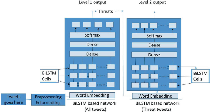

  

  The workflow of the proposed system model

  Fig. 3

  

  The BiLSTM-based neural network for level-1 classification

• In the proposed BiLSTM neural network, we used alternate combinations of hidden layers and hyper-parameter tuning, which allowed us to achieve a higher degree of accuracy.

• While there are various works in this domain that may classify threats, we designed our model to classify an endless number of threat categories with a single point of modification.

The section after that describes various similar works, followed by our proposed methodology in Sect. 3 with system workflow. In Sect. 4, we discussed the dataset and our system’s performance, followed by a conclusion and future scope in Sect. 5.

2 Related Work

In the study, Behzadan et al. [1] proposed a method for collecting tweets. They also put together a set of annotated datasets with 21,000 tweets. We used the same dataset for our work. Furthermore, they used Convolutional Neural Network to create a deep neural network that binary analyses tweets before classifying them into numerous threat subcategory classifications. The model work’s output receives an F1—score of 0.82, which is comparable to 82%. Bose et al. [3] focused on categorizing new occurrences that occur in the context of a cyber threat as a novel or developing. In several cases, they employed an unsupervised learning algorithm, which is rather uncommon. The ranking system developed as a result of this work is superior to any previously developed system. Their algorithm also includes a technique for ranking trending events as soon as they occur, ensuring that events that are innovative but not hot or widely tweeted do not lose their significance. After constructing the classifier, thirty manually annotated tweets were used to evaluate it, yielding an accuracy of 75% True Positive, 83.33% True Negative, and a precision of 93.75%. Sceller et al. [4] presented an automated approach that can detect and classify cyber threat-containing tools in real time in their study. Sonar is the name of the program they created. It’s a graphical tool that can provide real-time classification notifications as well as the geological location from which the tweets are coming. They fed their nearest neighbor algorithm with 47.8 million tweets. Furthermore, their technology is capable of comprehending not only English, but every language is spoken anywhere on the planet. Because the time complexity is O(c), or constant time, Sonar can provide real-time notifications. In the study, Le et al. [5] established the concept of threat intelligence collecting using tweets. They improved the novelty categorization by using a neural network. The primary purpose was to collect all cyber threat intelligence (CTI) and format it in a specific way. They adopted the same formatting as the CVE database, and they worked to ensure that the CVE is updated faster than it is now. They had a 64.30% accuracy rate. Their work was also compared to that of other researchers employing well-known approaches such as conventional SVM, CNN, and multi-layered perceptron (MLP), and it was discovered that their work provided greater precision and F1-score. In the research, Dionísio et al. [6] created a model that can binary classify tweets and then utilize named entity recognition to further classify them into their appropriate classification. They’ve developed a deep neural network-based processing pipeline for a revolutionary tool. After separating the dataset into three parts, they collected data for four months and used it for training, testing, and validation. They employed CNN and produced a True Positive rate of 94% and a True Negative rate of 91%, which is much higher than many other models. Their model also gets a 92% F1-score for the NER service it delivers. We discovered that the accuracy obtained by the systems described above is less. Many researchers have sought to improve threat classification, but we have proposed a system that allows us to classify threats over a wide range of categories, compared to currently available systems. In comparison to the previous research, we attained substantially higher classification accuracy.

3 Proposed Methodology and System Workflow

3.1 Data Collection

We largely used a standard dataset compiled by [1]. As previously said, anyone who uses Twitter is sitting on a gold mine waiting to be discovered. The Twitter Intelligence API, abbreviated as ‘TWINT,’ was utilized. TWINT is a python-based library that may be easily imported, and installation instructions can be found online. Behzadan et al. [1] used TWINT’s filters to only use tweets from firms classed as DDOS, Ransomware, Botnet, Vulnerability, Leak, and so on.

The following subsections detail the proposed system’s design. Figure 1 depicts the primary workflow of our proposed approach. The system components are shown in greater detail in Fig. 2. The BiLSTM cells (small rectangle blocks), which are effectively two LSTM employed one for forward computation and the other for backward computation, are depicted in Fig. 2. In addition, the proposed system is based on the work of [7].

3.2 Implementation

As previously stated, we employed BiLSTM in this project. We started by importing the data. Because the data was derived from tweets, some preprocessing was required, such as the removal of punctuation, special characters, and mentions, among other things [8,9,10]. After that, lemmatization [11] and tokenization [12] were used. As we all know, lemmatization scrapes a word by its postfix, thus related terms like ‘simple’, ‘simpler’, and ‘simplest’ all have the same weight, which could have resulted in an error in the weight computation of individual words. Tokenization is another useful step since it splits strings into meaningful tokens, which helps the computer calculate the weight of the words as a sequence more accurately use for further vectorization. Following that, the data was sent to the neural network model via the embedding layer, which created the embedding matrix using the glove model [3]. The two dense layers are then followed by stacked BiLSTM layers utilized for computation. The activation function was employed by the SoftMax layer on top to determine the final output class. Over 30 epochs, we iterated the training process and were able to obtain high accuracy.

The split dataset is used to create the second classification model in level-2, which only includes the ‘Threat’ categories from the level-1 classifiers. We found 9341 tweets that were rated as ‘threat’ level-1 on Twitter (actual 8351 threat tweets are available in dataset). They were used to train our level-2 classification model, which has a similar fundamental structure to the first (see Fig. 2). As a result, we were able to achieve the best possible training accuracy.

Algorithms for cyber threat classification from Twitter using BiLSTM-based deep neural network are given below for both the levels. Figures 3 and 4 also show the deep neural network architecture for the same.

Fig. 4

The layered structure of the proposed classifier with the BiLSTM

Algorithm 1

The multi-class tweet classification Level-1 Classification (coarse-grained).

Input: Tweets.

Output: Multi-class labeling of tweets.

Step 1: Input tweets, t.

Step 2: Pre-process and format t.

Step 3: Vectorize the tweets.

Step 4: Learning the model using BiLSTM-based neural network as per Fig. 3.

Step 5: Determine the final class (output) label (threat, marketing, irrelevant, or unknown).

(SoftMax determines the maximum probable outcome as final class)

Algorithm 2

The Level-2 Classification (fine-grained) for threat subcategorization.

Input: Threat-containing Tweet Stream.

Output: Threat subcategorization of tweets.

Step 1: Save the captured tweets, t.

Step 2: Pre-process t.

Vectorize the tweets and add padding to them.

Step 3: Train the deep learning model using the tweets as per Fig. 4.

Step 4: Determine the final class (output) label.

(SoftMax determines the maximum probable outcome as final class)

Overview of the proposed BiLSTM-based neural network. Next, we describe the different components and layers of our BiLSTM-based neural network. The BiLSTM architecture [13,14,15] is made up of memory blocks or LSTM cells, which are recurrently connected network modules. A standard BiLSTM classifier computes the hidden vector sequence h = h₁, h₂…, hT and the output class Y given an input sequence x = x₁, x₂, …, xT. The equations that make up the model are as follows.

$$\underset{{h}_{i}}{\to }={\mathrm{LSTM}}_{\mathrm{fw}}\left(\underset{{h}_{i-1}}{\to },{x}_{i}\right)$$

(1)

$$\underset{{h}_{i}}{\leftarrow }={\mathrm{LSTM}}_{\mathrm{bw}}\left(\underset{{h}_{i+1}}{\leftarrow },{x}_{i}\right)$$

(2)

$$\delta =\mathrm{drop}\left(\underset{{h}_{i}}{\to },\underset{{h}_{i}}{\leftarrow }\right)$$

(3)

$$y=\mathrm{softmax }\left(\left[\underset{{h}_{i}}{\to },\underset{{h}_{i}}{\leftarrow }\right]\right)$$

(4)

For the classification job, the T + 100-layer model is utilized, which is based on the state-of-the-art BiLSTM presented in [15]. Finally, as a Softmax layer, we added a multi-class classifier to classify the operation. Figure 3 shows the level-1 (coarse-grained) classification for all the tweets.

Figure 4 shows the level-2 (fine-grained) classification for the tweets belong to the threat category.

Embedding layer. The initial layer of our neural network architecture is this layer [9, 11, 16]. The primary goal of this layer is to convert the words into fixed-size vectors. First, using pre-trained word vectors, the word problem is turned into a vector [17, 18]. To produce the sequence of input from the word problem, the widely utilized Glove word embedding [16] is employed. The embedding layer vectorizes, as the name implies. The embedding layer employs the embedding matrix, a large chunk of data that has been successfully generated and dubbed the Glove model. This is one of the most effective vectorization techniques. The following parameters are used: the input dimension is the size of individual words, the output dimension is 100, the input length is the sequence length of words in a sentence, the weights are [embedding matrix], and Trainable is False.

BiLSTM layer. As previously stated, the layer is the heart and soul of our neural network, performing all of the heavy liftings. BiLSTM (Bidirectional Long Short-Term Memory) [13,14,15] is an advancement over standard Recurrent Neural Networks (RNN). BiLSTM is a model for processing sequential data available that is among the best. Backpropagation is one of the two methods for minimizing error or optimizing loss. This is how the neural network best understands the sequences and aids in further classification. Even when the amount of data accessible is limited, BiLSTM makes efficient use of it by traversing it back and forth. The following parameters were used: Return sequence = True, weight = 10.

Dense Layer. The dense layer is a deep-connected neural network layer [19], meaning that each neuron in it receives input from across all neurons in the previous layer. The dense layer produces an ‘m’ dimensional vector as its output. As a result, the dense layer is mostly employed to alter the vector’s dimensions. Some other essential hyper-parameters used in the proposed system are given below.

• 1. hidden units are 16 and activation function is ‘ReLu,’ ReLu works with the formula: $G\left(z\right)=\mathrm{max}\{0,z\}$

• 2. hidden units are 64 and activation function is ‘ReLu,’ ReLu works with the formula: $G\left(z\right)=\mathrm{max}\{0,z\}$

• 3. hidden units = 4 and activation function = ‘softmax,’ Softmax works with the formula: ${\sigma (\underset{Z}{\to })}_{i}= \frac{{e}^{{Z}_{i}}}{\sum_{j=1}^{K}{e}^{{Z}_{j}}}$

  Where, ‘σ’ represents Softmax output, ‘e’ represents exponential, ‘z’ represents token count, ‘j’ represents iteration variable, ‘K’ represents learning rate, and finally ‘t’ represents bias.

Optimizer. We used Adam optimizer [20, 21] for our neural network except for the layers. It optimizes very efficiently and is based on the stochastic gradient descent (SGD) principle [22]. When we received noisy data, we utilized Adam optimizer to optimize the neural network model. It automatically modifies network weights and biases, making the model more efficient. During the training of the neural network model, we additionally implemented an early halting mechanism based on parameter value loss [23] to avoid gaining poorer accuracy. This works beautifully and has a track record of success.

Loss function. The loss function of our neural network was also controlled using ‘categorical_crossentropy’ [8]. In categorical cross-entropy, the loss function is determined as the difference between the expected probability and the actual classes. After putting it to use, we were able to surpass the 80% threshold. Figure 5 shows the training loss and accuracy of our proposed level-1 annotator. We were able to achieve the model’s training accuracy of 81.53% and use it to achieve further heights in the following categorization. Figures 5, 6, and 7 show the training and validation accuracy and loss over the no of epochs for our level-1, level-2, and level-2 followed by level-1 (denoted as level 1→2), respectively. Although we achieved adequate training accuracy and loss, due to the lack of a good quality dataset, validation accuracy and loss are not satisfactory.

Fig. 5

Training accuracy (left) and loss (right) over the epochs for level-1 classification task

Fig. 6

Training and validation accuracy (left) and loss (right) over the epochs for level-2 classification task

Fig. 7

Training and validation accuracy (left) and loss (right) over the epochs for level 1→2 classification task

4 Dataset and Result

4.1 Results

The model evaluation takes a lot of time and effort. We were able to produce a good functional model after a lot of trial and error. Behzadan et al. [1] manually labeled the dataset with the four-category system that our classifier had been trained to recognize, ‘Irrelevant,’ ‘Business,’ ‘Threat,’ and ‘Unknown’. The dataset originally has 21,487 data entries. There are 8351 threats, 4881 irrelevant data, 3967 business/marketing data, and 4288 unknown data among the total. Out of the total threat category tweets, 2094 were DDoS, 372 leak, 1759 general, 1778 vulnerability, 1276 ransomware, 358 botnet, and 714 0day tweets are present. However, a total of 9341 tweets were classified as threats after the level-1 classification was tested on the entire dataset of 21,487 tweets, and they were used as input for the level-2 classifier (see Fig. 2). In both classifiers, we kept the train-test split at 70:30 and the validation split at 20%. We got 88.08% accuracy on the 30% test data we separated. We got 88.16% test accuracy in level-1 on the whole dataset. This is an acceptable outcome. The level-2 classifier was trained using the ‘Threat’ predicted tweets from our level-1 classifier. The tweets were classified as follows: ‘vulnerability,’ ‘ransomware,’ ‘DDoS,’ ‘leak,’ ‘General,’ ‘0day,’ and ‘botnet.’ The final accuracy, we achieved in level-2 is 73.26% (followed by level-1). Detailed result analysis and evaluation are given in the next subsection.

4.2 Result Analysis and Evaluation

Following the effective completion of our job, we were able to obtain a clear picture. Our pipeline threat classifiers were producing positive findings. For the text classification approach, we employed standard evaluation criteria as shown below.

Accuracy: The accuracy with which classifier predictions are made. True Positive and True Negative represent the classifiers’ correct predictions.

$$\mathrm{Accuracy }= \frac{(\mathrm{True \, positive }+\mathrm{ True \, Negetive})}{(\mathrm{True \, Positive }+\mathrm{ True \, Negative }+\mathrm{ False \, Positive }+\mathrm{ False \, Negative})}$$

Precision: The number of positive findings that are correct. It demonstrates how many data instances have been correctly classified and which are true.

$$\mathrm{Precision }= \frac{\left(\mathrm{True \, positive}\right)}{\left(\mathrm{True \, Positive }+\mathrm{ False \, Positive}\right)}$$

Recall: This is the classifier’s correct prediction.

$$\mathrm{Recall }= \frac{\left(\mathrm{True \, positive}\right)}{\left(\mathrm{True \, Positive }+\mathrm{ False \, Negative}\right)}$$

The test accuracy at level-1 is 88.08% on the test dataset (30% split), and 88.16% on the whole dataset. Figure 8 shows the confusion matrix for the final level-1 classification on the test dataset, which has a precision of 88.13% and a recall of 88.08%.

Fig. 8

Level-1 confusion matrix (0 = irrelevant, 1 = business, 3 = threat, 4 = unknown)

According to our proposed method (see Fig. 2), we were able to achieve 88.14% training accuracy and 86.91% validation accuracy in the level-2 classifier with 9341 tweets classified as ‘threat’ from level-1, which also contains false positive in another 3 categories, all labeled as ‘other’ subcategory (means there is no threat involved). The ultimate accuracy, precision, and recall were 81.71% (the final accuracy of level 1→2), 78.93%, and 81.68%, respectively. The confusion matrix for level 1→2 classifications is shown in Fig. 9. Where 0 denotes ‘other,’ 1 denotes ‘leak,’ 2 denotes ‘general,’ 3 denotes ‘vulnerability,’ 4 denotes ‘DDoS,’ 5 denotes ‘ransomware,’ 6 denotes ‘0day,’ and 7 denotes ‘botnet.’ ‘Other’ subcategory is part of the ‘marketing,’ ‘irrelevant’, and ‘unknown’ categories which are wrongly classified as ‘threat’ category by our level-1 classifier as false positives.

Fig. 9

Level-1→2 confusion matrix

Given the manually separated 8351 threat tweets, we were able to attain 96.90% training accuracy and 95.19% validation accuracy with the level-2 classifier (used standalone). We ended up with a testing accuracy of 90.06%, precision of 90.41%, and recall of 90.06%. This was a huge advance above previous methods. The level-2 classification’s confusion matrix is shown in Fig. 10. Where 0 denotes a ‘leak,’ 1 denotes a ‘general,’ 2 denotes a ‘vulnerability,’ 3 denotes a ‘DDoS,’ 4 denotes a ‘ransomware,’ 5 denotes a ‘0day,’ and 6 denotes a ‘botnet’.

Fig. 10

Level-2 confusion matrix

4.3 Performance Comparison

Our level-1 classifier finally achieved a threat classification accuracy of 88.08%, while the threat classification done by [1] achieved a test accuracy of 87.56% (see Table 2). At level 1, [1]’s work was more accurate than ours, scoring 87.56% versus 88.08%. However, no proper comparison can be performed because [1] only did binary classification (Threat or not), but we did multi-class classification into four categories in our level-1 classification, and this dataset hasn’t been used by any other researchers, so no comparisons can be made. Behzadan et al. [1] did not perform level-2 classification further, therefore no comparison is possible. Table 2 shows the performance comparison.

Table 2 Performance comparison with a similar system on the same dataset for level-2 classification

5 Conclusion

We have successfully made a system model which is better and faster compared to another available system. We used a novel methodology to achieve a better performance. Now to increase the accuracy anymore, more data would be required to train the model. The work will be further extended with the attention mechanism to achieve better accuracy. We are working on adding more features to identify cyber threats in tweets. The code will be publicly available in GitHub. Dionísio et al. [24] in his work has introduced the concept of Multitask Learning which can be implemented in this work in the future. Multitask learning is a concept that makes use of the trained hidden layer of one classification to help increase the accuracy of the next one. This concept is really great. We have found some unique attention parameters which we are already working on to make even more remarkable contributions in this domain hence fulfilling our motto to make the internet a safer place for all. We intend to expand the model’s ability to classify threat-containing tweets into additional subcategories in the future, as well as introduce novel attention parameters that will have a stronger impact on this field. Since hackers have stepped up their game, security researchers must also step up their game and put in significant effort to prevent any further crimes from occurring. We’re also looking into measures to stop these tweet-based threats from spreading further. As we all know, simply classifying tweets is a task, but it is incomplete unless they are prevented from spreading. As a result, as part of our ongoing research, we’re looking into integrating some cyber-security techniques that can be used to prevent threat tweets from being retweeted or viewed by most people if they violate specific rules.

References

Behzadan V, Aguirre C, Bose A, Hsu W (2018) Corpus and deep learning classifier for collection of cyber threat indicators in Twitter stream. In: 2018 IEEE international conference on Big Data (Big Data), pp 5002–5007. https://doi.org/10.1109/BigData.2018.8622506
https://www.mathworks.com/help/deeplearning/ref/nnet.cnn.layer.bilstmlayer.html
Bose A, Behzadan V, Aguirre C, Hsu WH (2019) A novel approach for detection and ranking of trendy and emerging cyber threat events in Twitter streams. In: Proceedings of the 2019 IEEE/ACM international conference on advances in social networks analysis and mining (ASONAM ‘19). Association for Computing Machinery, New York, NY, USA, pp 871–878. https://doi.org/10.1145/3341161.3344379
Sceller Q, Karbab E, Debbabi M, Iqbal F (2017) SONAR: automatic detection of cyber security events over the Twitter stream. pp 1–11. https://doi.org/10.1145/3098954.3098992
Le B-D, Wang G, Nasim M, Ali Babar M (2019) Gathering cyber threat intelligence from Twitter using novelty classification. pp 316–323. https://doi.org/10.1109/CW.2019.00058
Dionísio N, Alves F, Ferreira PM, Bessani A (2019) Cyberthreat detection from Twitter using deep neural networks. In: 2019 international joint conference on neural networks (IJCNN), pp 1–8. https://doi.org/10.1109/IJCNN.2019.8852475
Fang Y, Gao J, Liu Z, Huang C (2020) Detecting cyber threat event from Twitter using IDCNN and BiLSTM. Appl Sci 10:5922. https://doi.org/10.3390/app10175922
Attarwala A, Dimitrov S, Obeidi A (2017) How efficient is Twitter: predicting 2012 U.S. presidential elections using support vector machine via Twitter and comparing against Iowa Electronic Markets. In: Intelligent systems conference
Zong S, Ritter A, Mueller G, Wright E (2019) Analyzing the perceived severity of cybersecurity threats reported on social media. arXiv e-prints
Pennington J, Socher R, Manning CD (2014) GloVe: global vectors for word representation. In: Proceedings of the empirical methods in natural language processing
Wagner C, Dulaunoy A, Wagener G, Iklody A (2016) MISP: the design and implementation of a collaborative threat intelligence sharing platform. In: Proceedings of the 2016 ACM on workshop on information sharing and collaborative security (WISCS). Association for Computing Machinery
Collobert R, Weston J, Bottou L, Karlen M, Kavukcuoglu K, Kuksa P (2011) Natural language processing (almost) from scratch. J Mach Learn Res
Sabottke C, Suciu O, Dumitras T (2015) Vulnerability disclosure in the age of social media: exploiting twitter for predicting real-world exploits. In: 24th USENIX Security symposium (USENIX Security 15)
Devlin J, Chang M-W, Lee K, Toutanova K (2019) BERT: pre-training of deep bidirectional transformers for language understanding. In: Proceedings of the 2019 conference of the North American chapter of the Association for Computational Linguistics: Human Language Technologies, vol 1 (long and short papers)
Graves A, Schmidhuber J (2005) Framewise phoneme classification with bidirectional LSTM and other neural network architectures. Neural Netw 18(5–6):602–610
Mikolov T, Chen K, Corrado GS, Dean J (2013) Efficient estimation of word representations in vector space
Kim Y (2014) Convolutional neural networks for sentence classification. arXiv e-prints
Hochreiter S, Schmidhuber J (1997) Long short-term memory. Neural Comput
Alves F, Ferreira PM, Bessani A (2019) Design of a classification model for a Twitter-based streaming threat monitor. In: 2019 49th annual IEEE/IFIP international conference on dependable systems and networks workshops (DSN-W)
Liu X, He P, Chen W, Gao J (2019) Multi-task deep neural networks for natural language understanding. In: Proceedings of the 57th annual meeting of the Association for Computational Linguistics
Baxter J (1997) A Bayesian/information theoretic model of learning to learn via multiple task sampling. Mach Learn 7–39
Liao X, Yuan K, Wang X, Li Z, Xing L, Beyah R (2016) Acing the IOC game: toward automatic discovery and analysis of open-source cyber threat intelligence. In: Proceedings of the 2016 ACM SIGSAC conference on computer and communications security
Ruder S, Bingel J, Augenstein I, Søgaard A (2017) Latent multi-task architecture learning. In: Proceedings of the AAAI conference on artificial intelligence
Dionísio N, Alves F, Ferreira PM, Bessani A (2020) Towards end-to-end cyberthreat detection from Twitter using multi-task learning. In: 2020 international joint conference on neural networks (IJCNN), pp 1–8. https://doi.org/10.1109/IJCNN48605.2020.9207159
Author information
Authors and Affiliations
Corresponding author
Editor information
Editors and Affiliations
Rights and permissions
Copyright information
© 2023 The Author(s), under exclusive license to Springer Nature Singapore Pte Ltd.
About this paper
Cite this paper
Harh, S., Mandal, S., Giri, D. (2023). Detection and Classification of Cyber Threats in Tweets Toward Prevention. In: Bhattacharyya, S., Koeppen, M., De, D., Piuri, V. (eds) Intelligent Systems and Human Machine Collaboration. Lecture Notes in Electrical Engineering, vol 985. Springer, Singapore. https://doi.org/10.1007/978-981-19-8477-8_8
Download citation
DOI: https://doi.org/10.1007/978-981-19-8477-8_8
Published:
Publisher Name: Springer, Singapore
Print ISBN: 978-981-19-8476-1
Online ISBN: 978-981-19-8477-8
eBook Packages: Computer ScienceComputer Science (R0)