Non-linear Schemes for Representation

Abstract

In this chapter we deal with various nonlinear feature extraction schemes. In nonlinear feature extraction, the extracted features may be viewed as nonlinear combinations of the originally given features. Two popular neural network architectures employed are self-organizing map (SOM) and autoencoder (AE). We examine both of them in this chapter.

5.1 Introduction

We have studied different schemes for representation in the earlier chapters. These include:

• Feature Selection: Here, we select a subset of size l from the given set of L(> l) features.

• Linear Feature Extraction: Under this category we represent each pattern using a collection of l(< L) features. Each of these l features is obtained by using an appropriate linear combination of the given L features.

In this chapter, we will deal with extracting features that may be viewed as nonlinear combinations of the given L features.

5.2 Optimization Schemes for Representation

Let X _i and X _j be two L-dimensional vectors. Let P _i and P _j be the respective vectors in the l-dimensional space. Let d _ij be the euclidean distance between P _i and P _j and let $d_{ij}^*$ be the distance between X _i and X _j. The idea behind the optimization is to minimize a function that captures the difference between d _ij and $d_{ij}^*$ over all the pairs of patterns.

The specific function used by the popular Sammon’s mapping algorithm is

$$\displaystyle \begin{aligned} \frac{1}{\sum_{i<j}d_{ij}^*}\; \sum_{i<j}\frac{(d_{ij}^*-d_{ij})^2}{d_{ij}^*}.\end{aligned}$$

In other words, this nonlinear mapping algorithm employs a nonlinear optimization algorithm that starts with an initial representation and keeps on updating by using a gradient descent approach. The idea behind the choice of the objective function is to preserve some structure of the data, given in high-dimensional space, after mapping the data to a lower-dimensional space.

If X is an L-dimensional vector and l = 2, then one possible initial representation of P, corresponding to X, in the two-dimensional space is given by

$$\displaystyle \begin{aligned} P=\begin{pmatrix}P_1\\P_2 \end{pmatrix} = \begin{pmatrix}\sum_{i=1}^L X_i\\ \sum_{i=1}^L X_i^2 \end{pmatrix}.\end{aligned}$$

This initial representation in the l-dimensional space (l = 2 here) is updated iteratively till some stopping/termination criterion is satisfied.

5.3 Visualization

• 1. Representation using Faces: Here, a pattern is represented using a face for easy visualization. It may be explained using the face shown in Fig. 5.1.

  Fig. 5.1

  

  An example face image representation of a pattern

  A three-dimensional pattern (L = 3) is represented as a face in the figure. The first feature f ₁ is used to depict the height of the face. The second feature f ₂ is used to represent the width of the face and feature f ₃ depicts the length of the mouth. Note that it is possible to incorporate more features. For example, f ₄ can be used to capture the size of the eyes; f ₅ for the length of the nose; f ₆ for the distance between the eyes; f ₇ for the distance between the eyes and the nose; f ₈ for the distance between the nose and mouth, and so on. In addition one can use other parts like ears to represent more features.

  So, such a representation of patterns using faces can help the users in discriminating between patterns from different classes.

• 2. Self-Organizing Map (SOM): Kohonen’s SOM is the most popular neural network model to represent a collection of L-dimensional vectors in a two- or three-dimensional space . Consider the simple two-dimensional network shown in Fig. 5.2.

  Fig. 5.2

  

  Kohonen’s SOM

  This network may be viewed as having the input and output layers. The input layer is an L-dimensional layer. An L-dimensional vector X is presented at the input layer. The L components of X are x ₁, x ₂, ⋯ , x _L as shown in the figure.

  The output layer typically is a two-dimensional grid of M × N cells. in the figure the values of M and N are 7 and 10 respectively. Every cell is connected to the input layer with L weights. For example, if the top leftmost cell is numbered as 1, then the input x _j is linked to this cell with a weight W _j,1 for j = 1, 2, ⋯ , L. Similarly ith cell (shown here using the third row from the top and the sixth column from the left) is connected using a collection of L weights. For example, the Lth input node is connected using the weight W _L,i as shown in the figure. We have shown weights connected to 3 out of 70 cells for the sake of clarity in the figure.

  So, if there are L inputs and M × N cells in the output layer, then there will be M × N × L weights to train. These weights are initially chosen randomly and are updated based on the assignment, of data presented, to the cells. For example, if a data vector X ^p is more similar to the weight vector, W(j) = (W _1,j, W _2,j, ⋯ , W _L,j), then X ^P is associated with the jth cell and the weight vector, W(j), associated with the winner cell (jth cell) is updated to align more with X ^p. Such an update ensures that when X ^p is presented next time it will match better with the weight vector W(j).

  Typically, the input data will be a collection of n data vectors, X ¹, X ², ⋯ , X ⁿ. These n data vectors are presented in a sequence at the input layer and the weight vector associated with the winning neuron is updated after assigning each pattern. These input vectors are repeatedly presented at the input layer multiple times (epochs). It is continued till either there are no updates to the weight vectors in an epoch or till a pre-specified number of epochs is completed. This may be viewed as associating each of the data vectors with a cell that is matching better in terms of its current weight vector.

  It is possible to view the entire activity as clustering the n patterns into clusters corresponding to the output cells. There are several variants that can be used:

  • In the procedure specified, weights of only the winning cell/neuron are updated . It is possible to update the weights associated with the neurons located within a window around the winning cell. Different window types were specified.

  • It is popularly used to cluster unlabeled patterns. However, it can be used to cluster labelled patterns also.

  • It may be viewed as mapping L-dimensional vectors into a two-dimensional map. It is shown to achieve the mapping so that topological properties of the data are preserved.

  Consider the first 250 patterns of class label 1 and 7 in the MNIST Test Data set. We set the default seed to the random generator, using the command rng default. We used MATLAB, selforgmap function with the following parameters

  • dimensions = [12, 12]

  • Number of training steps for initial covering of the input space, coverSteps = 100

  • Initial neighborhood size, initNeighbor = 3

  • Layer topology function (default = ‘hextop’)

  • Neuron distance function (default = ‘linkdist’)

  The obtained SOM is shown in Fig. 5.3. The 144 grid/neurons (12 × 12) are numbered on the top in Fig. 5.3. At each grid point, the patterns which are falling in the grid, are averaged (For example, if three patterns fall in a grid, those three images are added and divided by 3, to get the average 28 × 28 image/pattern). The averaged pattern is converted into a binary vector (if pixel value greater than 127, it is replaced by 1 else replaced by 0). We observe the following in Fig. 5.3,

  • In the last three rows, (grid numbered 109 to 144) the patterns are mostly inclined to the right.

    Fig. 5.3

    

    SOM for first 250 patterns in classes labelled 1 and 7 in MNIST Test dataset

  • Pattern in grid numbers 4–12 and 16–19 are mostly inclined to the left.

  • Patterns which are marked in red box are actually outlier patterns in the actual data set, not resulted from the addition of patterns falling in their respective grids.

  • There is a clear transition from 1 to 7, as we move from left to right.

  • It is able to capture the characteristics of different ones and sevens and clusters them together.

• 3. T-Distributed Stochastic Neighbor Embedding (T-SNE) Plot :

  This is a very popular visualization tool that employs a nonlinear mapping scheme to reduce the dimensionality of the data from l to 2. Given the data in the l-dimensional space, it estimates a probability structure over pairs of points. The probability is larger if the corresponding pair of points are similar and it is smaller if the two points are dissimilar. Similarly it computes the probability structure in the reduced dimensional space. KL-divergence between these two probability distributions is minimized to achieve the mapping.

  Let us consider all the test patterns of MNIST data set. Figure 5.4 shows T-SNE plot for all the test patterns of MNIST data set with Perplexity = 30 (for many values of Perplexity we got similar plots) and Euclidean Distance as distance measure using MATLAB-tsne function . We can observe that there are many overlaps between many class labels. For example, patterns from classes 1 and 7 show significant overlaps, similarly classes labelled 3 and 8 show overlaps. Let us consider only the patterns of classes labelled 1 and 7 respectively. Figure 5.5 shows the T-SNE for class labelled 1 and 7. We can clearly observe the overlapping patterns. From Fig. 5.5, we picked some overlapping patterns and displayed their corresponding high dimensional image values in Fig. 5.6. In Fig. 5.6, the first two patterns (in position (1,1) and (1,2) respectively), are actually labelled as pattern 1, but they occur in the region of label 7 and similarly other patterns with actual label as 7, but in the T-SNE plot in Fig. 5.5, they occur in the region of label 1 respectively.

  Fig. 5.4

  

  T-SNE for all test patterns in MNIST Data set

  Fig. 5.5

  

  T-SNE for patterns labelled 7 and 1 in MNIST Data-set

  Fig. 5.6

  

  Some overlapping pattern of class labelled 7 and 1 in MNIST Data set

  We took six misplaced patterns in the T-SNE plot in Fig. 5.5. For these six patterns, we found three nearest neighbors in the lower dimensional embedding and we plotted their corresponding higher dimensional input in Fig. 5.7. In Fig. 5.7, the first column represents the misplaced patterns and other columns correspond to their three nearest neighbors respectively.

  Fig. 5.7

  

  Three nearest neighbours of misplaced patterns

  For the same misplaced patterns (column 1 in Fig. 5.7), we find all the three nearest neighbors belonging to the same class. For example, for the pattern at position (1,1) in Fig. 5.7, the actual label of the pattern is label 7, we find the corresponding neighbors among all the patterns belonging to class label 7 and we plotted them as the first row in Fig. 5.8 and similarly for other patterns.

  Fig. 5.8

  

  Three nearest neighbours in the same class of misplaced patterns

  The T-SNE plots for test patterns labelled 7 and 1 show misplacement of patterns. So, in order to measure the effect of misplacement, in the lower dimensional embedding space a KNN classifier with nine nearest neighbors is used. For each pattern in the lower dimensional space, nine nearest neighbors are found and using Majority vote the label of the pattern is predicted from its nine nearest neighbors. If the predicted label is the actual label of the pattern, then that pattern is not misplaced in the T-SNE plot, else, the pattern is declared as a misplaced pattern. By the above mentioned criterion, the train accuracy (A) may give the measure of misplacement by the T-SNE plot.

  Various L-norms with parameter r, are used to compute the dissimilarity for the T-SNE plot. The Training Accuracy (A) for various values of parameter is tabulated in Table 5.1. From the table, we observe that for fractional norms and lower values of parameter r, there are many misplaced patterns in the T-SNE plots and as the value of r increase, the misplacement is getting reduced, which is reflected in terms of the increase in the training accuracy A.

  Table 5.1 T-SNE Error analysis for different values of r using Minkowski distance

  From Figs. 5.9 and 5.10, we observe the following:

  • For lower values of r, the distance measure in higher dimensions is large, but in the lower dimensional space, distance is small and the clusters are tightly packed. As the value of r increases, we can observe the reduction in within cluster distance and the clusters are becoming loose.

    Fig. 5.9

    

    T-SNE for various L-Norms

    Fig. 5.10

    

    T-SNE for various L-Norms

  • As the value of r increases, the clear separation between the two clusters is reducing.

  • The penetration of pattern labelled 7 (blue) into the region of 1 (red) is getting reduced as the parameter r increases.

  • The occurrence of pattern labelled 7 (blue) in far extreme end in the regions of 1 (red) is getting reduced as the value of r increases.

  • As r increases, the misplacement of patterns is getting reduced.

  Consider Figs. 5.11 and 5.12 for further insights

  Fig. 5.11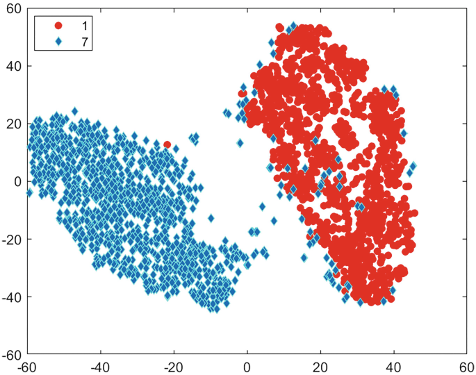

  

  T-SNE Plot with L-Norm r = 0.2

  Fig. 5.12

  

  T-SNE Plot with L-Norm r = 95

5.4 Autoencoders for Representation

let us consider the ORL face Data set . The Data set consists of 400 face images. The entire set of 400 faces is divided into 320 Train patterns and 80 test patterns, such that for each class label 8 patterns are assigned to the Training set and two patterns are assigned to the test set respectively. The image dimension is 112 by 92. Each image is converted into a row vector. So, the number of features of the Data set is 10, 304 = 112 ∗ 92. For the sake of simplicity and computation capacity constrains, we consider a single hidden layer Autoencoder and employed the following procedure for feature extraction and classification

• Each image is reshaped as 100 × 100 (instead of original dimension 112 × 92).

• Each reshaped image is divided into four quadrants, {C1, C2, C3, C4} of dimension 50 × 50 each.

• Four different single hidden layer Autoencoders{A1, A2, A3, A4} are used; each one extracts features from each quadrant,{C1, C2, C3, C4} of the image. The number of features is the number of neurons in the single hidden layer.

• The four sets of features {f1, f2, f3, f4} extracted from the four different Autoencoders{A1, A2, A3, A4}, are used for classification using a softmax classifier for each Autoencoder. (Note: Each Autoencoder and softmax-Pair are trained separately for their respective quadrants).

• For a given test pattern, its four quadrants are given as input to their corresponding Autoencoder-softmax Pair{A1, A2, A3, A4} and four class labels are predicted one for each quadrant.

• Using Majority voting among the four predicted class labels from the four individual Autoencoder-softmax-pairs, the class label for the test pattern is predicted.

• The Test Accuracy of each quadrant and for the entire image (predicted using Majority voting) is noted and the experiments are repeated for various values of the parameters of the Autoencoder.

Parameters of Autoencoder

Let us start with a brief introduction of a single layer Autoencoder. Consider the following notation,

• A single input vector x with dimension L, x $\in \mathbb {R}^{L}$.

• The total number of training patterns, N

• The entire training data matrix X $\in \mathbb {R}^{L \times N}$ of size L × N, where patterns are stacked column wise.

• The first layer of Autoencoder has l, hidden units (neurons).

• The weight matrix W ^(p) and bias vector b ^(p) at level (layer) p. (where p represents the number of levels/layers. We have considered only a single layer Autoencoder; so, we have two levels, level = 1 encoder level and level = 2 decoder level respectively).

• Let z $\in \mathbb {R}^{l}$ be the latent representation of single input vector x, with dimension l × 1

• Let Z $\in \mathbb {R}^{l \times N}$ be the latent representation of the entire input training data matrix, of size l × N (a matrix of size l × N).

• Let h(.) represent the non linear function at the encoder and decoder level which introduces the non linearity.

At the first level of Autoencoder, which is the encoder level, the single input vector $x \in \mathbb {R}^{L}$ is converted into its lower dimensional latent representation $z \in \mathbb {R}^{l}$ (where l < L) as follows:

$$\displaystyle \begin{aligned} z^{(1)} & = h\left(W^{(1)} \cdot x + b^{(1)} \right) \end{aligned} $$

$$\displaystyle \begin{aligned} z^{(1)} & = h\left( \begin{bmatrix} w_{1\:1}^{(1)} & w_{1\:2}^{(1)} & \dots & w_{1\:L}^{(1)} \\ \vdots & \ddots & \ddots & \vdots\\ w_{l\:1}^{(1)} & \dots & \dots & w_{l\:L}^{(1)} \end{bmatrix} \cdot \begin{bmatrix} x_{1}\\ \vdots\\ x_{L} \end{bmatrix} + \begin{bmatrix} b_{1}^{(1)}\\ \vdots\\ b_{l}^{(1)} \end{bmatrix} \right) \end{aligned} $$

where superscript (1) represents the first level (Encoder level) and W ⁽¹⁾ and b ⁽¹⁾ are the corresponding weight vector and bias terms at the encoder level.

At the second level, which is the decoder level, an estimate of the input vector x̂, is obtained as follows:

where superscript (2) represents the second level (decoder level) and W ⁽²⁾ and b ⁽²⁾ are the corresponding weight vector and bias terms at the decoder level. So, the Autoencoder takes an input vector of dimension L and reduces to a lower dimensional latent vector of dimension l; then it tries to reconstruct the estimate of input vector from the lower dimensional latent representation.

For illustration, consider an example single hidden layer Autoencoder in Fig. 5.13. In Fig. 5.13, we observe the following,

• The input nodes represents the input vector x with dimension L = 8.

  Fig. 5.13

  

  An example single hidden layer Autoencoder

• The middle hidden layer represents the latent vector z with dimension l = 4

• The output nodes represents the reconstructed estimate of input vector $\hat {x}$ with dimension L = 8.

• The edge weights are randomly selected and their thickness is propositional to their weights

Now, consider the following parameters, which are tuned for the experiments.

• 1. Hidden Layer Size (l):

  The number of hidden units (neurons) in the single layer Autoencoder is tuned by this parameter, Hidden layer size, l. As the number of hidden units increases the number of weights and bias parameters increases at both the encoder and decoder levels respectively.

• 2. Encoder-Decoder Transfer Function [TF]:

  We used non linear transfer functions for the encoder and decoder as follows:

  • Logistic sigmoid function, TF ₁

    $$\displaystyle \begin{aligned} h(k)& = \frac{1}{1+e^{- k}} \end{aligned} $$

  • Positive saturating linear transfer function, TF ₂

    $$\displaystyle \begin{aligned} h(k) = \left\{ \begin{array}{l l} 0 \hspace{1cm}& \text{if } k\leq 0\\ k\hspace{1cm}& \text{if } 0 < k < 1\\ 1\hspace{1cm}& \text{if } k \geq 1\\ \end{array}\right. \end{aligned}$$

  The Autoencoder reconstructs the input from the decoder level; so, the range of the input must match the range of the decoder transfer function. Hence, the inputs are scaled to match the range of decoder transfer function accordingly.

• 3. Maximum number of training epochs [MaxEpochs]

  The maximum number of training epochs/iterations is fixed as 500 because of computational constraints.

• 4. Cost Function, [CF]:

  The Autoencoder tries to reduce the Mean Square Error between the input vector $x \subset \mathbb {R}^{L}$ and the reconstructed estimate x̂ $\subset \mathbb {R}^{L}$; we can also add magnitude constraint to the weights and Sparsity constraint by employing a suitable Cost Function as follows:

  $$\displaystyle \begin{aligned} CF = MSE + \lambda \cdot \varOmega_{weights} + \beta \cdot \varOmega_{Sparsity} \end{aligned}$$

• 5. Mean Square Error [MSE]

  $$\displaystyle \begin{aligned} MSE = \frac{1}{N} \sum_{i}^{N}\sum_{j}^{L} \left( x_{ij} - \hat{x}_{ij}\right)\end{aligned}$$

  Where N represents the total number of Training patterns. L is the dimensionality of the training patterns and $\hat {x}$ represents the reconstructed estimate of the actual training pattern x by the Autoencoder.

• 6. L ₂ Weight Regularization Ω _weights:

  As the Autoencoder reduces the error between the actual training patterns and their estimates, we need to have the following:

  • a mechanism to control the magnitude of the weights.

  • to prevent the Autoencoder from remembering the training patterns and over fitting.

  Hence the following weight regularization term is used:

  $$\displaystyle \begin{aligned} \varOmega_{weights} = \sum_{l}^{P} \sum_{i}^{} \sum_{j}^{} \left( W_{i,j}^{(l)} \right)^{2} \end{aligned}$$

  where P is the total number of levels of the Autoencoder, as we have considered a single layer Autoencoder, we have P = 2. These are Encoder level and Decoder level. The number of elements of the Weight matrix W at each level varies. The Encoder level weight matrix W ⁽¹⁾ has a dimension L × l and Decoder level weight matrix W ⁽²⁾ has a dimension l × L. These weight matrices can be modified to incorporate the bias terms too.

• 7. L ₂ Weight Regularization term λ:

  Parameter which varies the contribution of L ₂ Weight Regularization term Ω _weights in the Cost function.

• 8. Sparsity Regularization, Ω _Sparsity:

  We can control the firing of a neuron by controlling its average output activation value. If the average output activation value of a neuron is low, it means that the neuron is responding (firing) only to the features present in a subset of training examples. The average output activation value of ith neuron, $\hat {\rho _{i}}$, is:

  $$\displaystyle \begin{aligned} \hat{\rho_{i}} = \frac{1}{N} \sum_{j = 1}^{N} h(W_{i}^{(p)} \cdot x_{j} + b_{i}^{(p)}) \end{aligned}$$

  where,

  • h(⋅) represents the Nonlinear Encoder-Decoder Activation function

  • $W_{i}^{(p)}$ represents the ith row of the weight matrix of level (p)

  • b _i represents the ith element of the bias term at level (p)

  So, we are calculating the average output of the activation function of ith neuron for all the training examples. We need to add a Kullback–Leibler divergence (KL) term to the Cost Function which results in a large value whenever the actual average output activation value of ith neuron deviates from the desired value ρ, by which we can introduce Sparsity in the latent representation.

  $$\displaystyle \begin{aligned} \varOmega_{Sparsity} & = \sum_{i} KL\left(\rho || \rho_{i}\right) & = \sum_{i} \rho \cdot \log \left( \frac{\rho}{\rho_{i}} \right) + \left( 1 - \rho \right) \cdot \log \frac{1-\rho}{1-\rho_{i}} \end{aligned} $$

• 9. Sparsity Regularization term, β:

  Parameter which varies the contribution of Sparsity Regularization term Ω _Sparsity in the Cost function.

The above mentioned parameters are varied and the results are tabulated in the next section.

5.5 Experimental Results: ORL Data Set

Let the notation for test accuracy of the four quadrants be TA1, TA2, TA3, and TA4 and final test accuracy for the entire image by Majority voting be TA. We have varied the parameter λ, Transfer function and the results are tabulated in Table 5.2. From Table 5.2, we observe that Positive saturating linear function (TF ₂) performs well when compared to Logistic sigmoid function (TF ₁) in terms of final test accuracy TA.

Table 5.2 λ Experimentation for ORL data set

Let us tune the parameter ρ, Transfer function and perform the experiment. The results are tabulated in Table 5.3. From Table 5.3, we again observe that TF ₂ outperforms TF ₁ in terms of final test accuracy TA.

Table 5.3 ρ Experimentation for ORL data set

Now, we alter the number of hidden neurons l along with ρ and Transfer function. The results are tabulated in Table 5.4.

Table 5.4 Hidden layer p—Experimentation for ORL data set

From the results we can observe the following:

• When the inputs are scaled properly, the Positive saturating linear function (TF ₂) performs well when compared to Logistic sigmoid function (TF ₁) in terms of final test accuracy TA.

• Increasing the number of dimensions, l, in the latent representation may not necessarily result in a better representation.

• By proper tuning of parameters, we can achieve better representation even with a smaller value of l, dimension of latent representation. For Example, in Table 5.4, for l = 600, we got better Test accuracy TA, than higher values of l.

5.6 Experimental Results: MNIST Data Set

Let us consider the patterns of classes labelled 7 and 9 from the MNIST data set. Each pattern is a 28 × 28 image, whose pixel values range from 0 to 255. Every pattern is converted into a binary row vector of dimension 1 × 784, such that a pixel value greater than 127 is replaced by 1 and pixel value less than or equal to 127 is substituted by 0. These row converted binary patterns are stacked to form the training set of size 12, 214 and test set of size 2037 respectively. Each pattern is a binary vector of length 784.

A single hidden layer Autoencoder is used as a feature extractor and Softmax layer is used as the classifier. The experiment mentioned in Sect. 5.4 is repeated for the MNIST Data set. As the dimension of the input vector is less (784 in the case of MNIST Data set), we have directly used the input vectors without pursuing any divide and conquer strategy as mentioned in Sect. 5.4.

The input image x (28 × 28 image as 1 × 784 vector) is fed into the Autoencoder and the reconstructed estimate x̂ is obtained. The Structural Similarity Index, SSIM between the input image x and its estimate x̂ is calculated for all the training and test patterns and its values are averaged. The SSIM is a good measure of reconstructing capability of the Autoencoder. The output parameters like Test Accuracy, averaged SSIM of training set and averaged SSIM of test set are tabulated for different experiments. The parameter MaxEpochs = 200 is fixed for all the experiments.

Fixing the parameter l, all other parameters are varied and the results are tabulated in Table 5.5. Similarly, fixing all other parameters as constant, parameter l is varied and the results are tabulated in Table 5.6.

Table 5.5 ρ Experimentation for MNIST data set

Table 5.6 Hidden layer l—Experimentation for MNIST data set

From Tables 5.5 and 5.6, we can again observe that the Positive saturating linear function (TF ₂) performs well when compared to Logistic sigmoid function (TF ₁) in terms of SSIM.

Figure 5.14 shows the reconstructed images of some patterns, where the Autoencoder used TF ₁ with ρ = 0.5 and λ = 0.01. Similarly, Fig. 5.15 shows the reconstructed images of some patterns using Positive saturating linear transfer function, TF ₂. From Figs. 5.14 and 5.15, we observe a better reconstruction capability of Positive saturating linear transfer function (Close to the famous ReLu function).

Fig. 5.14

Reconstructed images using Logistic sigmoid function, TF ₁

Fig. 5.15

Positive saturating linear transfer function, TF ₂

In order to understand how the weight matrix in the Encoder level represents certain features and how the parameter ρ affects the weight matrix, consider Figs. 5.16 and 5.17.

Fig. 5.16

Weight matrix with ρ = 0.05

Fig. 5.17

Weight matrix with ρ = 0.95

For an Autoencoder of 100 hidden neurons, each neuron is represented in a 10 × 10 grid in Figs. 5.16 and 5.17. Each grid unit represents the 784 weights for each neuron as an 28 × 28 image. For ρ = 0.05 in Fig. 5.16, the average output activation values is low so the weight images 28 × 28 in each grid is nearer to black region representing smaller values and the neurons will fire only for certain features.

Similarly, for ρ = 0.95, in Fig. 5.17, the weights are having higher values nearer to the white regions and no sharp characteristics when compared to Fig. 5.16.

5.7 Summary

In this chapter, we have considered nonlinear feature extraction. Here each extracted feature may be viewed as a nonlinear combination of the given L features. We have discussed and examined three different schemes; they are useful in both dimensionality reduction and visualization. Specifically, we have considered

• 1. Self-organizing neural network: It is popularly called the self-organizing map (SOM). It can be used to map high-dimensional data vectors into a two or a three dimensional space. It has some nice properties:

  • It preserves the topological structure present in the data.

  • It can be viewed as a neural network architecture for clustering. The clusters are perceived based on the self-organization property exploited by the training algorithm.

  • It is helpful in visualizing the data in a two-dimensional space that is easy for human consumption.

• 2. T-Distributed Stochastic Neighbor Embedding (T-SNE) Plot: It is popularly known as the t-SNE plot. It is a nonlinear technique for dimensionality reduction and visualization of high-dimensional data. Some of its features are:

  • It is the most popular embedding technique for visualization of high-dimensional data.

  • It is popular in analysing the embedding techniques employed in complex networks including social networks, chemical and biological networks.

• 3. Autoencoder: It is also a neural network architecture primarily used in nonlinear dimensionality reduction. Some of its features are:

  • Based on the type of activation function used by various neurons, it can work like a nonlinear feature extractor (nonlinear activation) or like PCA to perform linear feature extraction (linear activation).

  • It is found to be an apt tool when the classes are not linearly separable in the original feature space.

In each of the above cases, we have conducted experiments and reported the results using two benchmark data sets, the MNIST handwritten digits data set and the ORL face data set.

References

Burges, C.J.C.: A tutorial on support vector machines for pattern recognition. Data Mining Knowl. Discov. 2(2), 121–167 (1998)
Schölkopf, B., Smola, A.J.: Learning with Kernels. MIT Press (2001)
Rifkin, R.M.: Multiclass Classification, Lecture Notes, Spring08. MIT, USA (2008)
Witten, I.H., Frank, E., Hall, M.A.: Data Mining, 3rd edn. Morgan Kauffmann (2011)
Kohonen, T., Honkela, T.: Kohonen network. Scholarpedia 2(1), 1568 (2007)
van der Maaten, L.J.P., Hinton, G.E.: Visualizing data using t-SNE. J. Mach. Learn. Res. 9, 2579–2605 (2008)
Goodfellow, I., Bengio, Y., Courville, A.: Deep Learning. MIT Press (2016)
Author information
Authors and Affiliations
Rights and permissions
Copyright information
© 2023 The Author(s), under exclusive license to Springer Nature Singapore Pte Ltd.
About this chapter
Cite this chapter
Murty, M., Avinash, M. (2023). Non-linear Schemes for Representation. In: Representation in Machine Learning. SpringerBriefs in Computer Science. Springer, Singapore. https://doi.org/10.1007/978-981-19-7908-8_5
Download citation
DOI: https://doi.org/10.1007/978-981-19-7908-8_5
Published:
Publisher Name: Springer, Singapore
Print ISBN: 978-981-19-7907-1
Online ISBN: 978-981-19-7908-8
eBook Packages: Computer ScienceComputer Science (R0)