
Abstract
Wireless networking technology is used to access networks or connect with other user devices in a wireless medium. Wireless Local Area Network IEEE 802.11g is one of the standards of wireless technology. IEEE 802.11g is a Wi-Fi 3 standard, which was designed in 2003. This has the properties of both 802.11a and 802.11b. This paper analyses the performance of this protocol standard with single access point. The effects of varying data rates are observed on the delay, media access delay, queue size, and maximum throughput are analyzed. Simulations were performed using OPNET. Along with these, the analysis of access points using HTTP is done to analyze object and page response time and further voice data analyses were performed to perceive jitter, packet end-to-end delay (time taken by the packet from source to destination), traffic sent, and traffic received between the nodes.
Access provided by Autonomous University of Puebla. Download conference paper PDF
Keywords
1 Introduction
Multiple access control (MAC) protocol and physical layer are implemented at the MAC layer in IEEE 802.11 standard. Infrastructure and ad hoc networks are supported by this standard. The performance of a wireless network depends on constraints which includes data rates buffer sizes threshold and throughput.
1.1 WLAN- Physical Architecture
There are two types of architecture for WLAN:
1. Infrastructure less architecture 2. Infrastructure architecture
-
1.
Infrastructure less architecture:
This architecture is the simplest of WLAN configurations which is an autonomous WLAN and it is also known as an ad-hoc network. This contains a set of computers grouped with the help of a LAN client adapter. No access point is required in this kind of configuration. The Fig. 1 below shows this architecture.
Fig. 1 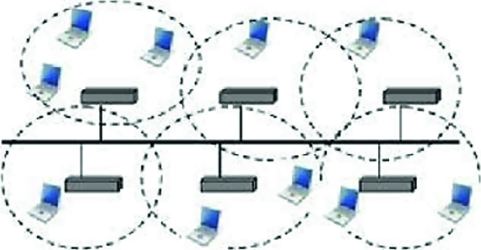
Infrastructure less wireless network

-
2.
Infrastructure architecture:
In this type of analysis, there is an access point present. These access points are connected with a distribution system like ethernet. These access points determine the cell and also define a confined radius over which the network has access. When a device moves out of one cell to another the connection with the new access point is made. This whole process is called handover. The architecture is s shown in the Fig. 2 below.
Fig. 2 
Infrastructure wireless network

2 References
In [2], the authors analyze the service availability, network performance, and user connection.
In [11], the authors have used DCF+ method to determine the performance of the network. This model provides a correct behavior of IEEE 802.11.
In [6], the authors have used opnet simulator to analyze the performance of IEEE 802.11g WLAN’s. Here they have studied the performance based on the number of workstations. The work is carried out on mobile as well as stationary stations to get a better understanding.
3 Selection of Access Point
3.1 Delay Analysis
A delay can be described as the time that exists between the time from when the packet was generated at the source to the time at which the packet reached the destination. So, in simple words, it’s the time that a packet takes to move in the network. The unit for this is seconds. This delay can be termed a packet end-to-end delay. This delay can also be caused due to latency. Latency refers to time taken by the packet from the required point to the destination. So, if this increases it implies that delay also increases.
The efficiency of network is determined by how fast the packet reaches the destination on time. Thus, if delay is minimum then the packet reaches the destination on time. So minimum delay means an efficient time flow.
3.2 Media Access Delay
This delay is described by the time from when the data reaches the MAC layer until it is successfully sent out to the wireless medium. This is important because in a real-time network if the data is not received within the required delay, then the data becomes useless. This delay should be as minimum as possible to provide an efficient real-time flow.
3.3 Queue Size
To study the performance parameters of a computer system queue size is the best. This will help provide explanations as to some of the issues like bottlenecks or compromised computer performance caused due to waiting for too long for the data to arrive.
3.4 Throughput
This is the most important parameter which is used to measure the amount of data that is transferred from source to destination within the given time frame. This can also be termed as the capacity of the network in bits per second or data per second. The throughput of a network helps in understanding the speed of the network.
Throughput gives the data transmitted per second. So if the throughput is high it can be concluded that the speed of the network is high/.
4 Software Requirement
OPNET simulator is one of the best simulators which provides a higher power and versatility. Due to its excellent features OPNET is chosen as the simulator. OPNET SIMULATOR
Opnet stands for Optimized network Engineering Tools which is a network simulator tool that is used to simulate the behavior and performance of any kind of network. Compared to other simulator tools Opnet has better power and versatility. This tool can be used to simulate a large area network with various protocols. This tool was built for military usage, but it has grown indefinitely for commercial simulation tools for networks. Though, it is an expensive software free licenses are available for the educational process. This tool defines network topology, nodes, and links that form the network. The processes that take place in a particular node and transmission link can also be user-defined. Opnet has a vast library set that provides simulation, and analysis of the network to compare the effect in different scenarios and the IDE of OPNET is user-friendly which makes the user use it with no issue.
5 Network Design
In this paper, a network is designed in such a way that there is one access point along with 15 nodes attached to it. The parameters considered here are throughput and delay.
The Fig. 3 above shows the network design.

Simulation model structure
6 Simulation Results
6.1 Delay Study
For the ‘delay’ parameter a study of 4 scenarios is considered and also when the data rate is increased from 1 to 54 Mbps, the delay decreases. The result shown below proves that as the data-rate increases the delay decreases. The Fig. 4 shows the delay comparison.

Delay comparison between 1 and 12 Mbps
6.2 Media Access Delay Study
As the data rate raises from 1 to 12 Mbps, the media access delay is decreased. Based on the graphical result shown below it is proved that the media access delay decreases with the increase in data-rate.
6.3 Queue Size Study
As the data rate raises from 1 to 12 Mbps, the queue size decreases. Theoretically, as the data-rate increases, the speed of data transmission from source to destination increases and the queue decreases. The graph below Fig. 6 proves the same in a practical scenario.
6.4 Throughput Study
When the data rate is increased from 1 to 12 Mbps the throughput increases. So as the data-rate increases the number of bits received also Figs. 5 and 6.

Media access delay

Queue size comparison between 1 and 12 Mbps
Increases thereby increasing the throughput of the system. The graph for the same is shown in the below Fig. 7.

Throughput comparison between 1 and 12 Mbps
7 Analysis of Access Point Using HTTP
Object Response time: provides the time that is taken to respond for every individual inlined object from the HTML page.
Page Response time: provides the time required to regain the entire page with all the contained inline objects as shown in Fig. 8.

Object and page response time
Figure 9 shows the traffic is sent and received in the network.

Traffic is sent and received in the network
8 Analysis of Voice Application Based on Different Parameters
-
1.
Jitter study: When two packets start at the destination point say at times t1 and t2 and reach the destination at a time t3, t4, then the jitter is expressed as jitter = (t4 − t3)–(t2 − t1) When the time difference at the destination node is less than that at the source node a negative jitter is formed.
From the above Fig. 10 we can see that different nodes experience different jitter. This is due to a packet getting queued or delayed anywhere in the network, where there was no delay or queuing for other packets.

Jitter in voice application
-
2.
Packet end-to-end delay:
Network delay is the delay caused when the sender node gives the packet at RTP and the receiver gets it at RTP. The encoding and decoding delay is computed from the encoder scheme and the latter is considered as same as that of the encoding delay.
From the above Fig. 11, it is observed that the Packet end-to-end delay is different for different nodes. This is due to variation in delay jitter experienced at different nodes in the network.

Packet end-to-end- delay in Voice application
-
3.
MOS Value: This gives the quality of voice and video sessions.
From the above plot, we can see that the MOS value for voice applications varies for different nodes due to variations in jitter, latency, and packet loss are shown in Figs. 12, 13 and 14.
Fig. 12 
MOS value of voice application
Fig. 13 
Traffic received in voice application (bytes/sec)
Fig. 14 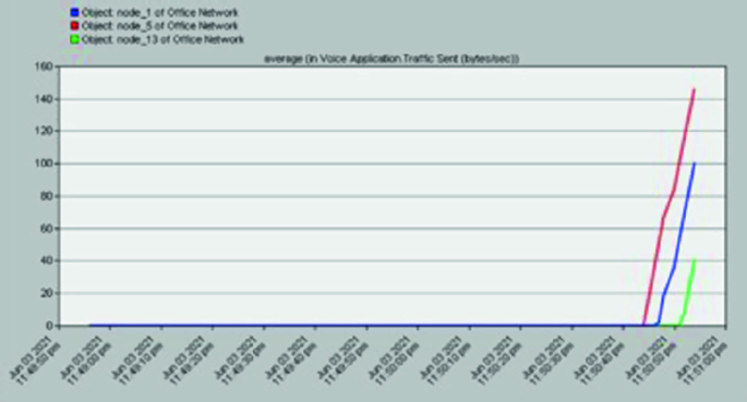
Traffic sent in voice application (bytes/sec)


9 Conclusion
In most of the research, the performance was analysed based on the number of workstations in the network. However, here in this paper the discussion is made on a wireless network based on various parameters. The paper here shows the design of the wireless network. The major challenges in such types of the network include delay, media access delay, queue size, and throughput. From simulations performed, the observations clearly show that when data rate is changed it effects other parameters also. From the results one can observe that when the data rate is raised the delay, Media access delay, and Queue size decrease whereas the throughput increases. This indicates that the data is delivered accurately and efficiently. Some of the parameters like MOS value, jitter, and packet end-to-end delay of Voice application are observed and found that they are interdependent.
References
Hamdan YB (2021) Construction of statistical SVM based recognition model for handwritten character recognition. J Inf Technol 3(02):92–107
Raj JS, Vijesh Joe C (2021) Wi-Fi network profiling and QoS assessment for real time video streaming. IRO J Sustain Wirel Syst 3(1):21–30
Karuppusamy P (2020) Effective test suite optimization for improving the coverage standards using hybrid wrapper filter memetic algorithm. J Soft Comput Paradigm 2(2):83–91
Dasgupta S, Roy PJ, Sharma N, Misra DD (2020) Application of IPv4, IPv6 and dual stack interface over 802.11ac, 802.11n and 802.11g wireless standards. In: Third international conference on advances in electronics, computers and communications (ICAECC) (2020)
Zuo PL, Peng T, Wu H, You K, Jing H, GuoW, Wang W (2020) Suppression of 802.11 transmission in 2.4 GHz ISM band: method and experimental verification. IEEE Xplore
Karki M, Shrestha A, Singh VL (2017) Performance comparision of IEEE 802.11g WLANs with respect to increasing number of workstation using OPNET modeler. In: International conference on computing and communication technologies for smart nation
Wahyuda DV, Achmadi YD, Sari RF (2017) Comparison of different WLAN standard on propagation performance in V2V named data networking. In: IEEE Asia Pacific conference on wireless and mobile
Wang T, Refai HH, Wang Q (2004) Performance analysis of the WLAN based on IEEE 802.11a/b/g standards in the presence of an interfering cordless phone. In: Henty BE, Rappaport TS (eds) IEEE 1st wireless and optical wireless network conference
Chatzimisios P, Boucouvalas AC, Vitsas V (2003) Influence of channel BER on IEEE 802.11 DCF. Electron Lett 39(23):1687–1689
Wu H, Cheng S, Peng Y, Long K, Ma J (2002) IEEE 802.11 distributed coordination function (DCF): analysis and enhancement. In: IEEE international conference on communications (ICC), vol 1, pp 605–609
Wu H, Peng Y, Long K, Cheng S, Ma J (2002) Performance of reliable transport protocol over IEEE 802.11 wireless LAN: analysis and enhancement. In: Proceedings of INFOCOM, vol 2, pp 599–607
Bianchi G (2000) Performance analysis of the IEEE 802.11 distributed coordination function. IEEE J Sel Areas Telecommun Wirel Ser 18:535–547
Author information
Authors and Affiliations
Corresponding author
Editor information
Editors and Affiliations
Rights and permissions
Copyright information
© 2023 The Author(s), under exclusive license to Springer Nature Singapore Pte Ltd.
About this paper

Cite this paper
Shreelatha, G.U., Kavyashree, M.K. (2023). IEEE 802.11g Wireless Protocol Standard: Performance Analysis. In: Joby, P.P., Balas, V.E., Palanisamy, R. (eds) IoT Based Control Networks and Intelligent Systems. Lecture Notes in Networks and Systems, vol 528. Springer, Singapore. https://doi.org/10.1007/978-981-19-5845-8_6
Download citation
DOI: https://doi.org/10.1007/978-981-19-5845-8_6
Published:
Publisher Name: Springer, Singapore
Print ISBN: 978-981-19-5844-1
Online ISBN: 978-981-19-5845-8
eBook Packages: EngineeringEngineering (R0)