
Abstract
Electric vehicle (EV) plays an important role to escape from environmental issues like increasing air pollution and limited stock of fossil fuel. EVs run on an electric motor, which is powered by its onboard rechargeable battery. EVs need a charging station to fulfil the energy demand of the battery. Recently, the penetration of EVs is increasing drastically in the modern power system. Therefore, the optimal planning of the electric vehicle charging stations (EVCSs) is necessary. The charging stations should maintain the power system parameters as well as it should provide services to the maximum EV users, which is a challenging job to the system planning engineers. However, the environmental benefits of EVs cannot be achieved if renewable energy resources are not incorporated into the system. The renewable-based distributed generation (DG) also helps to reduce the losses and improve the voltage profile of the system. Therefore, the distribution system with the charging stations must be renewably supported. However, the flow of EVs and generation from renewables are uncertain which is a matter of concern. This chapter describes the available planning for EVCSs in different distribution networks along with their methodologies. The results are also analyzed with their merits and demerits. The results of differenttypes of literature review show that the optimal allocation of charging stations helps to reduce the power loss of the distribution system as well asthe installation cost. Optimal allocation of DG contributes to additional power loss minimization. Moreover, technical information and specifications about EV and its charging infrastructure are presented in this chapter. The uncertain attributes associated with EV and DG are described. Also, the steps of different established methods to handle uncertainties are explained in this chapter.
Access provided by Autonomous University of Puebla. Download chapter PDF
Keywords
- Distribution network
- Distributed generation
- Electric vehicle
- Electric vehicle charging station
- Optimal planning
- Uncertainty
10.1 Introduction
10.1.1 Electric Vehicle
Vehicles with an internal combustion engine (ICE) run with fossil fuels and contribute to massive air and sound pollution. The electric vehicle is the solution for pollution less transportation system. EV also helps to stop the burden on fossils fuel consumption which is already at a diminished level. EV is based on an electric motor (EM) which is driven by a battery pack via a power converter. A three-phase induction motor and lithium-ion battery are mostly used in EV (Fathabadi 2019). The all-electric range (AER) is the distance that can be covered by an EV using only battery power with its full charge. The recent technologies have enhanced the EV driving range by more than 400 km in one charge (Al-Adsani et al. 2020). In broad, there are three types of EVs, which are shown in Fig. 10.1: (i) hybrid electric vehicle (HEV), (ii) plug-in hybrid electric vehicle (PHEV), (iii) battery electric vehicle (BEV).

Types of EV
-
(i)
HEV: This type of EV is having both an IC engine and electric motor, but the battery is not facilitated to charge from an external power supply. The battery takes charge from the braking system of the vehicle, called regenerative braking. The electric motor gives support to the IC engine to drive the vehicle as per requirement, that’s why it is called “hybrid”. The battery capacity of HEV is around 6 kWh (Iclodean et al. 2017).
Example: Honda Civic Hybrid, Toyota Prius Hybrid, Toyota Camry Hybrid, etc.
-
(ii)
PHEV: This is also a hybrid vehicle with an IC engine and electric motor, like HEV. Additionally, the battery of PHEV can be charged from regenerative braking as well as from external power, that’s why it is called “plug-in”. The battery capacity of BEV is around 100 kWh (Iclodean et al. 2017).
Example: Chevy Volt, Hyundai Sonata, Toyota Prius, etc.
-
(iii)
BEV: Only electric motor and battery are present in this type of vehicle. The battery is charged by the external EV charger. BEV also may be supported with regenerative braking. As there is no IC engine, therefore, the motor rating and battery capacity are quite higher than other types of vehicles. The battery capacity of BEV is around 5 kWh (Iclodean et al. 2017).
Example: BMW i3, Nissan LEAF, Tesla Model S, etc.
10.1.2 EV Charging
The charging station is mandatory to charge the EV, as nowadays most of the vehicles are PHEV and BEV. EVCSs are connected to the nodes in the distribution network. There are few standards for the connector of EV charger, such as CHAdeMO, Society of Automotive Engineers (SAE), International Electromechanical Commission (IEC) and Combined Charging System (CCS) (Trentadue et al. 2018). Furthermore, the EV charging facilities can be categorized as per the charging rate, Fig. 10.2 present the different levels of EV charging. CHAdeMO is the most popular among those for DC fast charging (Ahmadian et al. 2020).

Classification of EV charging level
However, the health of the batteries should be kept in mind, therefore, the SOC limits of EV’s battery are maintained for all the scenarios. Typically, 20% is the lower level of the SOC and 90% is the upper level, which is maintained (Pal et al. 2021). Charging efficiency and discharging efficiency are taken as 95 and 90%, respectively, for the simulation work with EV (Pal et al. 2021). Rating and uses of different charging levels according to SAE are as follows (Ahmadian et al. 2020):
-
Level 1: Single-phase AC 120 V, current 12–16 Amp, power 1.44–1.92 kW. This charging level is used for home charging and parking lot charging.
-
Level 2: Single/three-phase AC 240 V, current up to 80 Amp, power up to 19.2 kW. This charging level is used for the public charging station as well as home charging.
-
Level 3: DC 200–450 V, current up to 80 Amp, power up to 36 kW. This is particularly applicable only for the public charging station. The DC fast charging of CHAdeMO is with 50–500 V, current up to 125 Amp and output power up to 50 kW (Aziz and Oda 2017).
During charging, EV takes power from the grid, which is termed as “grid to vehicle”. Whereas, “vehicle to grid” technology provides the facility to feed power from EV to power system grid. V2G is beneficial for EV users and service providers along with the grid (Ma et al. 2012). EV owners can trade the power with the grid according to the real-time prices. The service providers can gain revenue from the dividend. The grid can mitigate the peak power demand from EVs and able to improve the node voltages when it is required. The rate of discharging during V2G is 2–4 kW (Pal et al. 2021). The drawback of the V2G is the battery degradation due to additional cycles of charging and discharging.
There is another solution for charging the EV batteries, i.e. battery-swapping station (BSS). In BSS, a charged battery is exchanged with a nearly empty battery of EV. The BSS is not much convenient because more batteries are required and annoyed users about nonidentical batteries’ health.
10.1.3 Distributed Generation
Distributed generation is a small-scale generation typically renewable-based, connected to the nodes of the distribution network. As DGs are installed near to the loads, therefore, it can supply the power locally to the load and helps to reduce the power losses as well as to improve the voltage profile of the distribution system (Pal et al. 2020). As the main motto of EVs is to reduce emissions, therefore, the conventional thermal power plant should not be utilized to charge the EVs. Incorporating renewable-based DG such as solar photovoltaic (PV), wind generators, will help to reduce pollution to some extent. However, the sizes and locations of DG in the distribution network are most significant to minimize maximum possible loss along with improvement of the voltages. Moreover, unplanned DG allocation may lead to undervoltage or overvoltage. The locations and demand of EVCSs can influence the allocation of DGs. Hence, simultaneous solution or two-layered optimization for EVCSs and DGs allocation is required to make optimal renewable supported distribution system including EVCSs. Many literature consider that DGs are connected with the EVCS. However, in case of renewable-based DG, uncertainties are a big issue to design the system optimally. Also, RESs are non-dispatchable generations that may require BES to store the surplus power and to utilize it as per requirement.
10.1.4 Uncertainty
Uncertainties are the critical concern to achieve realistic solutions for the research problem with EV and PV along with existing loads. The driving pattern of EVs and solar irradiance are the uncertain parameters for the EVCSs and DG power outputs. The uncertain parameters related to EV are:
-
(i)
Arrival Time (hh:mm): The time when an EV arrives at a charging station, is termed as the arrival time of that particular EV.
-
(ii)
Arrival SOC (%): The amount of SOC remaining of an EV at the moment of arrival at EVCS is called the arrival SOC of that EV.
-
(iii)
First Trip Distance (km): The distance covered by the EV before coming to the charging station.
-
(iv)
Subsequent Trip Distance (km): Expected distance will be travelled by the EV after getting charged from the EVCS.
-
(v)
Departure SOC (%): It is the desired SOC level by the EV, in other words, SOC of the EV while leaving the EVCS after charging. Departure SOC depends on the STD.
-
(vi)
Energy Requirement (kWh): It is the energy demand by the EV, which will be fulfilled from the EVCS. Energy demand is calculated from SOC at arrival, SOC at departure and battery capacity of the EV.
-
(vii)
Departure Time (hh:mm): The time when EV departs the EVCS after getting its desired charge. It depends on the energy requirement by the EV and the rate of charging/discharging.
The uncertain parameters related to PV power output are i) Solar Irradiance, ii) Temperature.
There are many established uncertainty handling methods that are able to take the uncertainties into consideration and provide accurate solutions. K-mean algorithm, Monte Carlo simulation and 2 m point estimation method are widely used stochastic tools to deal with uncertainties.
10.1.5 Highlights of the Chapter
This chapter presents the planning procedure of EVCSs with DGs and analyzed the results of different planning of EVCSs. To formulate the problem for EVCS allocation, some basic knowledge is necessary, which are given in the introduction section as:
-
Basic information of electric vehicle and its types with specifications.
-
Technical information about EV charging facility with its specifications and different levels.
-
Benefits of distributed generation.
-
Uncertainties associated with EVs and PVs.
The mathematical formulations, methodologies and results from different literature are shown and discussed in this chapter as:
-
Calculation of different parameters of EV and load at EVCS.
-
Objective functions to allocate EVCS and DG.
-
Constraints related to distribution network, EV, EVCS and DG.
-
Flow chart to solve allocation problem using optimization technique.
-
Different methods to handle uncertainties.
-
Result analyses of EVCS and DG allocation in different distribution networks for various objectives.
10.2 Related Work
There are many works related to EVCS allocation. Some of them provide realistic solutions considering different practical parameters. In Pal et al. (2019), fast-charging stations are placed optimally in IEEE 33 distribution system. The distribution network is divided into three zones to allocate EVCS. The power loss is minimized using grey wolf optimizer and results are confirmed using whale optimization algorithm. In Cui et al. (2019), ECVSs are located in the distribution network in view of practical factors associated with the urban area. In Deb et al. (2019), EVCSs are placed in Guwahati highway where multi-objective problem is formulated and solved using soft-computing techniques. In Dong et al. (2019), EVCS allocation is executed in London city. The EVCSs are allocated in the roads of the U.S. in He et al. (2019). Various optimization techniques are applied in Zhang et al. (2019) to obtain the locations of EVCS by taking care of area-wise charging demand. In Kong et al. (2019) and Guo and Zhao (2015), the optimal locations of EVCS are determined in Beijing. Conditions-based place selection for EVCS is performed in Hosseini and Sarder (2019). Again, (He et al. 2018) is also a distinguished investigation where EVCSs are planned on different roads and maps of cities.
In Awasthi et al. (2017), a hybrid optimization is used to allocate EVCSs in the Allahabad distribution network by minimizing installation cost and maximizing power quality. In Mehta et al. (2019), EVCSs are placed in a 33 bus distribution network by two-layer optimization. In Shojaabadi et al. (2016), EVCSs are planned considering the demand-side response. EVCSs are installed at optimal places with optimal sizes in Aljaidi et al. (2019). Charging station set-up is found out optimally in Davidov and Pantoš (2019) by various cost minimizations. In Yi et al. (2019), optimal locations and sizes are found out for EVCS. The costs related to EVCS instalment and operation are minimized in Liu and Bie (2019) and (Andrade et al. 2020) by allocating at optimal places. In Zhang et al. (2019), road networks and distribution networks are overlaid to find out the appropriate locations of the EVCS using soft-computing techniques. In Zhang et al. (2019), optimal locations of EVCS are determined in Beijing city to minimize power loss of the electrical network and EVCS cost. Optimal charging/discharging scheduling is achieved along with optimal EVCS locations in Hadian et al. (2020). In Pal et al. (2021), EVCS and DG are allocated simultaneously in the radial distribution network. The problem is solved using two-layer optimization. The uncertainties associated with EVs and DGs are taken care of. The results show that DG helps to increase voltage profile and to reduce the energy loss of the distribution system. It can be observed that optimal locations of EVCS reduce the energy loss. Also, locations influence the total land cost for the EVCSs.
In Pal et al. (2021), EVCSs are placed optimally in 33 radial distribution network which is merged with a road network. Multi-objective problem is formulated where energy loss, voltage deviation, last cost are minimized and weightage of the location is maximized. The results show that allocated EVCSs are distributed in the road network to serve the users suitably. In Shaaban et al. (2019) and Atat et al. (2020), EVCSs, as well as DGs, are located optimally. In Pal et al. (2021), a superimposed network is used to allocate EVCS which is taken as a public fast-charging station. Renewable-based DGs (PV) are also allocated optimally to minimize more loss of energy and to enhance the voltages of the distribution network. BESs are incorporated with PV to manage the variable renewable generation and variable load demand. BESs are also optimally scheduled. Moreover, EVs are assigned at apt EVCS considering their routes and traffic congestions. The BESs are also installed with EVCS in Dai et al. (2019), Yan et al. (2017), Gong et al. (2019), Kasturi et al. (2020). Allocation of EVCS and BSS is performed on a 15-bus and 43-bus network in Zheng et al. (2014). In Moradijoz et al. (2013), parking lots are placed in a distribution network. Again in Ahmadi et al. (2021), parking lots are optimally planned in IEEE 69 network with the appropriate charging strategies of the EVs to reduce the total costs associated with a parking lot. Also, in Liu et al. (2020)–(Ponnam and Swarnasri 2020), EVCSs are planned optimally in the distribution system.
The EV movement and charging requirement are uncertain parameters for this type of work. In Sokorai et al. (2018), the uncertainty of daily usages of EVCSs is modelled using the Markov chain’s tool. In Yi et al. (2019), uncertainties are handled using an artificial immune algorithm to find out the EVCS locations. K-means clustering method is applied in Shaaban et al. (2019) to look into uncertainties associated with DG and EV. MonteCarlo simulation-based algorithm is established in Andrade et al. (2020) to get the uncertain EV driving pattern for the allocation of EVCS. MCS is applied in Shojaabadi et al. (2016); Shojaabadi et al. 2016) to tackle the uncertainties related to EV. Still, these methods have drawbacks such as computational time, mathematical complexity, hard to deal with huge uncertain variables (Saha et al. 2019). 2 m PEM has many advantages over other techniques, which are used in Pal et al. (2021), (2021), (2021) to deal with uncertainties for EVCS allocation.
10.3 Problem Formulation
10.3.1 Mathematical Calculation of EV Parameters
The load at any charging station depends on the number of vehicles that are in charging/discharging mode and the rate of charging/discharging. The calculation of total load \(\left({EvL}_{S}^{\left(t\right)}\right)\) on \({S}\)th EVCS due to EVs at tth time is calculated as follows (Pal et al. 2021):
where \({C}_{r}\) and \({D}_{r}\) charging and discharging rate of G2V and V2G, \({nv}_{G2V}^{(t)}\) and \({nv}_{V2G}^{(t)}\) are number of vehicles in G2V mode and V2G mode, respectively, at \({t}\)th time. The energy demand \(\left({Req}_{v}^{eng}\right)\) by the \({v}\)th vehicle is determined as
where \({Req}_{v}^{soc}\), \({Req}_{v}^{eng}\) and \({Bc}_{v}\) indicate required SOC in %, required energy in kWh and battery capacity in kWh of \({v}\)th vehicle, respectively. \({\eta }_{ch}\) and \({\eta }_{dis}\) are charging and discharging efficiency of EV, respectively. The required SOC \(\left({Req}_{v}^{soc}\right)\) and required time \(\left({Req}_{v}^{time}\right)\) to charge the \({v}\)th vehicle is calculated as
\({Req}_{v}^{soc}\) is positive when departure SOC \(\left({D}_{v}^{soc}\right)\) is more than arrival SOC \(\left({A}_{v}^{soc}\right)\), that means the EV is connected in G2V/charging mode. If the value is negative, the state of EV is V2G/discharging. The arrival SOC \(\left({A}_{v}^{soc}\right)\) can be found by
where \({ftd}_{v}\) is the first trip distance which is travelled by the EV to come to the EVCS and \({AER}_{v}\) is the all- electric range of the \({v}\)th EV. The departure SOC \(\left({D}_{v}^{soc}\right)\) and departure time \(\left({D}_{v}^{time}\right)\) of \({v}\)th vehicle is calculated as (Pal et al. 2021)
where \({STD}_{v}\) is the subsequent trip distance of \({v}\)th vehicle. 20% is the minimum SOC level that should be maintained, to be specific, the departure SOC should not be less than 20%. The STD is obtained by (8), where \({td}_{v}\) is the total distance is covered by the EV.
In the above mentioned calculations, arrival time, first trip distance, total travel distance, AER and the battery capacity are the input parameters.
10.3.2 EVCS and DG Allocation
To allocate the EVCSs and DGs in the distribution system, the total load due to EVCS and generation from DG need to be calculated. If \({S}\)th EVCS and DG are connected at \({bu}\)th node in the distribution network, the total load \(({P}_{bu})\) on that node at \({t}\)th hour can be expressed as
where \({ExL}_{bu}^{(t)}\) is the existing load at \({bu}\)th node. \({EvL}_{S}^{(t)}\) is load due to EVCS at \({t}\)th time period which is obtained by (1). \(D{G}_{S}^{(t)}\) is the power generated from DG at time \(t\). The EVCS load and DG generation would be zero if they are not connected at bus \(bu\).
10.3.2.1 Objectives for the Allocation Problem
Different objectives are considered in various research works to allocate EVCS in the distribution network as well as traffic network. Maximization/minimization problem depends on the type of objective functions, such as electrical loss and instalment cost due to EVCSs being minimized and service to the users being maximized.
-
The total cost of EVCSs is minimized in Liu et al. (2013) considering the costs for operation and maintenance, investment and power loss to place the EVCSs at optimal locations. The mathematical objective function for the planning of EVCSs in the distribution network is expressed in Liu et al. (2013) as follows:
$$\mathrm{min}\left(F\right)=\sum_{t=1}^{T}\frac{1}{{\left(1+\eta \right)}^{t}}\left[\sum_{i=1}^{{N}_{EVCS}}{C}_{EVCSi}^{I}\left(t\right)+{C}_{EVCSi}^{O}\left(t\right)+{C}_{EVCSi}^{M}\left(t\right)+{C}_{PS}^{L}\left(t\right)\right]$$(10.10)where \({C}_{EVCSi}^{I}\left(t\right),{C}_{EVCSi}^{O}\left(t\right)\) and \({C}_{EVCSi}^{M}\left(t\right)\) are the instalment cost, operation cost and maintenance cost of \({i}\)th EVCS at \({t}\)th time period. \({C}_{PS}^{L}\left(t\right)\) is the cost of the power loss in the system at \({t}\)th time. \(\eta\) is the discount rate for reverse calculation of upcoming price, \({N}_{EVCS}\) is the number of EVCS is being allocated and \(T\) is the total project period.
-
For allocation of EVCSs. three objectives are considered in Wang et al. (2013) to cover maximum EV users by the EVCSs with keeping power losses and voltage deviations minimum. The multi-objective problem is converted to a single objective function by multiplying weighting factors \(\left({\alpha }_{1},{\alpha }_{2},{\alpha }_{3}\right)\) as below.
$$\mathrm{min}(F)=\mathrm{min}\left({\alpha }_{1}{F}_{1}+{\alpha }_{2}{F}_{2}+{\alpha }_{3}{F}_{3}\right)$$(10.11)where (11) is a minimization problem and \({F}_{1},{F}_{2}\) and \({F}_{3}\) are the normalized values of three objective functions. The objective functions as follows:
$$\mathrm{max}({F}_{1})=\sum_{q\in Q}{f}_{q}{y}_{q}$$(10.12)$$\mathrm{min}({F}_{2})={P}_{Loss}\left({U}_{i}{P}_{Si},{U}_{i}{Q}_{Si}\right)$$(10.13)$$\mathrm{min}({F}_{3})=\sum_{i=1}^{{N}_{d}}\frac{\left|{V}_{i}-{V}_{0}\right|}{{V}_{0}}$$(10.14)where \({F}_{1}\) is to serve the maximum number of EV by the EVCSs. \({F}_{2}\) and \({F}_{3}\) are to minimize power loss and voltage deviation of the distribution network, respectively. \({f}_{q}\) is the EV flow on \({q}\)th road, \(Q\) is the total number of roads and \({y}_{q}\) is binary variable for the response of all EVs, served or not. Binary \({U}_{i}\) denotes EVCS is connected at \({i}\)th bus or not,\({P}_{Si}\) and \({Q}_{Si}\) are the real and reactive power drawn by the EVCS at \({i}\)th bus.\({V}_{0}\) and \({V}_{i}\) are the rated voltage and the voltage at bus \(i\), respectively. \({N}_{d}\) a total number of buses present in the system.
-
The EVCSs are allocated in Awasthi et al. (2017) taking multi-objective problem (15) consisting of minimization of active and reactive power loss along with EVCS cost and maximization of voltage improvement index.
$$\min (F) = \min \left\{ {\frac{1}{{w_{1} VPII_{i} + w_{2} PLRI_{i} + w_{3} QLPI_{i} }}} \right\}(i \in NC)$$(10.15)where \({w}_{1},{w}_{2}\) and \({w}_{3}\) are the weighting coefficients to make a single objective problem to multi-objective and \(NC\) is the total number of charging stations to be allocated. \(I{C}_{i}\) is the initial cost for \({i}\)th EVCS and \({X}_{i}\) is binary variable is 1 if the EVCS is connected at \({i}\)th bus, otherwise 0. \(VPI{I}_{i},PLR{I}_{i}\) and \(QLP{I}_{i}\) are the indexes at \({i}\)th bus for improvement of voltage problem, reduction of active power loss and reduction of reactive power loss, respectively, as shown below.
$$VPI{I}_{i}=\frac{1}{\alpha +{\mathrm{max}}_{i=1}^{n}\left(\left|1-{V}_{(C{S}_{i})}\right|\right)}$$(10.16)$$PLR{I}_{i}=\frac{{P}_{L\left(base\right)}-{P}_{L\left(C{S}_{i}\right)}}{{P}_{L(base)}}$$(10.17)$$QLP{I}_{i}=\frac{{Q}_{L\left(base\right)}-{Q}_{L\left(C{S}_{i}\right)}}{{Q}_{L(base)}}$$(10.18)$$I{C}_{i}={C}_{in}+25{C}_{land}.{N}_{i}+{C}_{p}.{C}_{dev}.\left({N}_{i}-1\right)$$(10.19)where \({V}_{(C{S}_{i})}\) is the voltage of bus \(i\) once the EVCSs are connected and \(\alpha\) is a scalar variable. \({P}_{L\left(base\right)}\) and \({Q}_{L\left(base\right)}\) are the active and reactive power loss respectively at \({i}\)th bus without any EVCS and \({P}_{L\left(C{S}_{i}\right)}\) and \({Q}_{L\left(C{S}_{i}\right)}\) are the active and reactive power loss respectively at \({i}\)th bus after placing the EVCS. \({C}_{in},{C}_{land},{C}_{p}\) and \({C}_{dev}\) are investment cost, land cost, rated power of connector and development cost of connector, respectively, for charging station.
-
In Pal et al. (2021), multi-objective function is considered for EVCS allocation, which is transformed to a single objective as a minimization problem by applying weighting coefficients \(\left({\omega }_{1},{\omega }_{2},{\omega }_{3},{\omega }_{4}\right)\) as follows:
$$\mathrm{min}\left(F\right)=\mathrm{min}\left({\omega }_{1}{f}_{1}+{\omega }_{2}{f}_{2}+{\omega }_{3}{f}_{3}-{\omega }_{4}{f}_{4}\right)$$(10.20)where \({f}_{1}, {f}_{2},{f}_{3},{f}_{4}\) are the four objective functions, which are expressed below
$${\mathrm{min}(f}_{1})=\sum_{t=1}^{24}\sum_{br=1}^{{N}_{br}}{\left({I}_{br}^{\left(t\right)}\right)}^{2}\times {R}_{br}$$(10.21)$$\mathrm{min}({f}_{2})=\sum_{t=1}^{24}\sum_{bu=1}^{{N}_{bu}}\left|1-{V}_{bu}^{(t)}\right|$$(10.22)$${\mathrm{max}(f}_{3})=\sum_{S=1}^{{N}_{S}}{w}_{S}$$(10.23)$$\mathrm{min}({f}_{4})=\sum_{S=1}^{{N}_{S}}{c}_{S}$$(10.24)where \({f}_{1}\) is energy loss and \({f}_{2}\) is voltage deviation of the distribution system, \({f}_{3}\) is weightage of the locations of EVCS and \({f}_{4}\) is the land cost for installing EVCSs. \({I}_{br}^{\left(t\right)}\) is current flowing through branch \(br\) at time \(t\), \({R}_{br}\) is the resistance of \(b{r}\)th branch. \({V}_{bu}^{(t)}\) is the voltage of bus \(bu\) at time \(t\). \({w}_{S}\) and \({c}_{S}\) are the weightage and land cost of the \({S}\)th EVCS’s location, respectively. \({N}_{br}\), \({N}_{bu}\) and \({N}_{S}\) are the total number of branches, number of buses and number of EVCS, respectively.
-
In Mozafar et al. (2017), minimization of a multi-objective problem is formulated involving four objectives, i.e. power loss, voltage fluctuation, EV charging cost and battery degradation cost.
$$\mathrm{min}(F)=\mathrm{min}\left(\tau {f}_{1}+\beta {f}_{2}+\gamma {f}_{3}+{\alpha f}_{4}\right)$$(10.25)where \(\tau ,\beta ,\gamma\) and \(\alpha\) are the weighting factors, set as 0.4, 0.3, 0.2 and 0.1, respectively. \({f}_{1},{f}_{2}\) are the objective functions for power loss and voltage fluctuation for 24 h, which can be calculated as (21, 22), respectively. \({f}_{3}\)is the objective function for the cost of charging (G2V) including benefits from discharging (V2G) and \({f}_{4}\) is for downgrading costs of battery, as follows:
$${f}_{3}=\sum_{t=1}^{24}\left({P}_{sub,t}\times {\pi }^{TOU}\right)+{f}_{ch}-{f}_{dc}$$(10.26)$${f}_{4}=\frac{{C}_{b}.BCAP+{C}_{r}}{{L}_{c}.BCAP.DOD}{P}_{dc}^{PHEV}$$(10.27)where \({P}_{sub,t}\) is power from the substation at time \(t\). The dynamic electricity price is \({\pi }^{TOU}\).\({f}_{ch},{f}_{dc}\) are the cost for charging and profit from discharging (V2G). \({C}_{b},{C}_{r}\) and \({L}_{c}\) are the battery cost, cost for battery replacement and lifecycle of the battery, respectively, \(BCAP\mathrm{ and}DOD\) is the battery capacity and depth of discharge, respectively. \({P}_{dc}^{PHEV}\) is the energy discharged by the PHEV during V2G.
-
Single objective function is taken in Alhazmi et al. (2017) to maximize the coverage of the charging station to the EV users by allocating EVCS at proper places. The maximization problem is presented in Alhazmi et al. (2017) as
$$\mathrm{max}\left(F\right)=\mathrm{max}\sum_{i=1}^{{N}_{T}}T{D}_{i}{w}_{i}$$(10.28)where \(T{D}_{i}\) is the demand by the EV transportation at \({i}\)th location and \({w}_{i}\) is 1 if demand is fulfilled by the EVCS, otherwise 0.\({N}_{T}\) is the total nodes in the transportation network.
-
In Kandil et al. (2018), charging stations for PEVs are assigned along with renewable-based DG and battery energy storage. The yearly cost of energy is minimized to find out the appropriate locations, as follows:
$$\begin{aligned} \mathrm{min}\left(F\right) &= {\mathrm{min}}_{{\Omega }_{1},{\Omega }_{2}}{\sum }_{s}Pr{o}_{\left(s\right)}\times \\ & \left({\sum }_{i}\left[{C}_{RE\left(i\right)}-{R}_{RE\left(i,s\right)}+{C}_{ES\left(i\right)}+{C}_{EV\left(i\right)}\right]+\left[{C}_{loss\left(s\right)}+{C}_{cons\left(s\right)}\right]\right) \end{aligned}$$(10.29)where \({\Omega }_{1},{\Omega }_{2}\) are the installation and operation variables, respectively,\(Pr{o}_{\left(s\right)}\) is the probability of \({s}\)th scenario. \({C}_{RE\left(i\right)},{C}_{ES\left(i\right)}\) and \({C}_{EV\left(i\right)}\) are the capital investment and running costs for renewable energy, energy storage and EV charging station, respectively, connected at \({i}\)th bus. \({R}_{RE\left(i,s\right)}\) is the profit from renewable power generation. \({C}_{loss\left(s\right)},{C}_{cons\left(s\right)}\) are the energy loss cost and energy consumption cost by the loads, respectively.
-
DGs and EVCSs are allocated in Liu et al. (2020) using two-level optimization, where both levels are maximization problems. The objective function (30) of the upper level is consisting annual return \(\left({C}_{pro}\right)\), power loss cost \(\left({C}_{loss}\right)\) and environmental benefit \(\left({C}_{env}\right)\).
$$\mathrm{max}\left({F}_{upper}\right)={C}_{pro}-{C}_{loss}+{C}_{env}$$(10.30)The objective function in lower-level optimization is
$$\mathrm{max}\left({F}_{lower}\right)={C}_{l,S}+{C}_{l,B}-{C}_{l,OM}-{C}_{l,loss}+{C}_{l,env}$$(10.31)where \(l\) is the probabilistic scenario, \({C}_{l,S}\) denotes profit from the utility,\({C}_{l,B}\) represents government support for renewable generation, \({C}_{l,OM}\) is the operation and maintenance cost of EVCS and DG, \({C}_{l,loss},{C}_{l,env}\) are the power loss and environmental benefit, respectively.
-
Authors in Luo et al. (2020) propose a cost minimization objective considering DG and EVCS for optimal allocation. The total annual cost in the objective function involves the cost of investment \(\left({C}^{I}\right)\), operation and maintenance cost \({(C}^{O\&M})\), fuel cost with carbon emission \({(C}^{F\&E})\), electricity purchase cost from utility \(\left({C}^{P}\right)\), power loss cost \({(C}^{NL})\), energy loss for charging/discharging of EV \({(C}^{CL})\) and battery degradation cost \({(C}^{B})\), as
$$\mathrm{min}\left(F\right)=\mathrm{min}\left({C}^{I}+{C}^{O\&M}+{C}^{F\&E}+{C}^{P}+{C}^{NL}+{C}^{CL}+{C}^{B}\right).$$(10.32)
10.3.2.2 Constraints for the Allocation
Different constraints are considered related to EV, charging station, traffic network and distribution system for EVCS and DG allocation. Some required constraints are presented below.
-
Constraint Related to Distribution Network
-
Constraint for power flow balance: This is a compulsory condition that need to be satisfied for any distribution network at any point of time. The total power supplied from substation and DGs should be equal to total power loss and total load including EVCSs, can be written as:
$${P}_{sub}+{P}_{DG}-{P}_{loss}-{P}_{load}=0$$(10.33)where \({P}_{sub},{P}_{DG},{P}_{loss}\) and \({P}_{load}\) are the power from substation, power from DG, power losses in the system and load, respectively.
-
Constraint for node voltages: To provide quality power to the users, the voltage of the nodes of the distribution network should be maintained within permissible limits as (34) where \({V}^{min}\) and \({V}^{max}\) are the lower and upper limit of the bus voltage. respectively.
$$V^{\min } < V_{bu} < V^{\max }$$(10.34) -
Constraint for line currents: This constraint is for a limit of the current flow through each branch because of the conductors’ maximum current carrying capacity \({(I}^{max})\) as
$$\left|{I}_{br}\right|<{I}^{max}$$(10.35)
-
Constraint Related to EVCS
-
The constraint for the number of ports: Number of maximum and minimum ports in an EVCS can be restricted according to EV demand and power supply capacity of distribution node as (Awasthi et al. 2017)
$${N}_{i}^{min}\le {N}_{i}\le {N}_{i}^{max}, i=\mathrm{1,2},\dots ,{N}_{EVCS}$$(10.36)where \({N}_{i}\) is the number of the port at \({i}\)th charging station, \({N}_{i}^{min}\) and \({N}_{i}^{max}\) are the minimum and maximum limit, respectively. \({N}_{EVCS}\) is the number of EVCS in the system.
-
Constraint for EVCS power: The total power drawn by the EVCSs in a distribution system should be limited by permissible level because of the supply capacity of the distribution system as (Liu et al. 2013)
$$\sum\nolimits_{i = 1}^{{N_{EVCS} }} P_{EVCSi} \le P_{EVCS}^{\max }$$(10.37)where \(P_{EVCSi}\) power is drawn by the \(i\)th EVCS and \({P}_{EVCS}^{max}\)is the maximum permissible limit.
-
Constraint Related to EV
-
Constraint for EV’s SOC: The SOC level of the EV has to be within limits (38) because overcharge or overdischarge impacts the battery health (Pal et al. 2021).
$$SO{C}^{min}\le SOC\le SO{C}^{max}$$(10.38)where \(SO{C}^{min}\) and \(SO{C}^{max}\) are the lower and upper limit of the SOC which should be maintained in the EV battery.
-
Constraint Related to DG
-
Constraint for DG power: The DG output power should not exceed the maximum limit because it may cause over voltage, high short circuit current and reverse power flow (Pal et al. 2020). The constraint is shown below, where \({P}_{DGi}\) is the power generated from \({i}\)th DG and \({N}_{DG}\) is the total number of DG presence in the system.\({P}_{DG}^{max}\) is the maximum allowable power which can be penetrated from the DGs.
$$\sum\nolimits_{i = 1}^{{N_{DG} }} {P_{DGi} } \le P_{DG}^{\max }$$(10.39)

Flowchart of the generalized algorithm of EVCS allocation using optimization technique
10.3.2.3 Generalized Algorithm of EVCS Allocation
A simple algorithm is illustrated in Fig. 10.3 to allocate the EVCSs using the optimization technique. First, the locations are generated randomly in the initialization stage. Then the locations are updated using an optimization algorithm to minimize/maximize the objective function. If all the constraints are satisfied then only the solution is acceptable. The updating procedure is stopped when the convergence criteria are reached.
10.4 Uncertainty Modelling
In the allocation problem of EVCS and DG, the EV flow and PV power output are not deterministic variables. Researchers have to take care of the uncertain variables to find out the optimal locations, otherwise, the solutions would not be applicable in a practical scenario. The Monte Carlo simulation, K-mean algorithm and 2 m point estimation method are the established method to handle the uncertain variables.
-
K-mean algorithm: In Liu et al. (2020), K-mean + + algorithm is employed for uncertain variables such as PV, wind power output and load demand. In this technique, the number of uncertain scenarios is reduced by the clustering process using historical data. The procedure is given below as (Liu et al. 2020):
-
(i)
The historical original data of uncertain variables (PV output, EV charging demand) are normalized.
-
(Ii)
Total \(K\) number of clustering centres \(\left({\xi }_{1},{\xi }_{2},{\xi }_{3},\dots ,{\xi }_{K}\right)\) are created as follows:
-
(a)
A random set is selected from the original 365 number of sets \(\left({N}_{i},i=\mathrm{1,2},3,\dots ,365\right)\) for the 1st cluster \(({\xi }_{1})\).
-
(b)
The shortest distance is calculated between \({N}_{i}\) and \({\xi }_{1}\), i.e. \(d\left({N}_{i},{\xi }_{1}\right)\). A summation of all distances \((d)\) is needed.
-
(c)
A random distance is generated which is less than \(\mathrm{sum}(d)\) and it is updated to \(d\left({N}_{i},{\xi }_{1}\right)\). \({N}_{i}\) will be the new centre of the cluster if the random distance is less than 0.
-
(d)
Repeat step b and c to select \(K\) number of centres \(\left({\xi }_{1},{\xi }_{2},{\xi }_{3},\dots ,{\xi }_{K}\right)\).
-
(e)
The distances between remaining original sets to centres of the clustering. The original sets are allocated to the nearest cluster.
-
(f)
The centres of \(K\) number of cluster are found out and new generations’ centres are updated.
-
(g)
Repeat step c and d till clustering are unchanged.
-
Monte Carlo simulation: The authors in Kandil et al. (2018) have applied a Markov chain-based MCS to capture uncertain arrival time and departure time of the EVs. The MCS model is used in Alhazmi et al. (2017) to tackle the uncertainties of travel distance by the EVs and energy remain in EVs’ batteries. The simple steps are:
-
(i)
Generate random numbers of the uncertain variables from their distribution function.
-
(ii)
Make numerous sets with the random numbers as different scenarios.
-
(iii)
Solve the problem for each scenario with a fixed deterministic set.
-
(iv)
The average value of the results of all scenarios is taken.
-
2 m point estimation method: This method is utilized in Pal et al. (2021) to handle the uncertainties of arrival time, arrival SOC and travelling distance of the EVs. In this method, dual scenarios are created for each uncertain variable using a distribution function based on past data. The major steps are as follows:
-
(i)
Generate two random values of each uncertain variable using distribution function and central moment.
-
(ii)
Make two sets with a random value and mean value for a fixed deterministic set.
-
(iii)
Repeat step 1 and 2 for all the uncertain variables. The total number of the set will be double the number of uncertain variables.
-
(iv)
Solve the problem for each set with a fixed deterministic set.
-
(v)
Determine the mean value of the outcomes from all sets.
10.5 Result and Discussion
-
In Pal et al. (2019), fast-charging stations are allocated in IEEE 33 radial distribution network. The whole network is divided into separate zones, where each EVCS is placed at each zone optimally as Fig. 10.4. In this work, the power loss of the distribution network is minimized. The locations are 2, 21 and 30, which are scattered in the area. The power loss after optimal allocation of EVCS is 234.6 kW for 30 EVs. The voltage profile of the distribution network is shown in Fig. 10.5 after zone-wise allocation of EVCSs. It is seen that the voltage of each node maintains permissible 10% limits.
Fig. 10.4 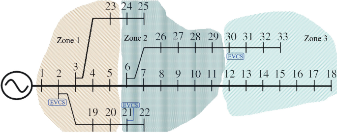
Allocation of fast-charging station in IEEE 33 node system (Pal et al. 2019)
Fig. 10.5 
Voltage profile of IEEE 33 node system after optimal allocation of EVCSs (Pal et al. 2019)
-
EVCSs are placed optimally on IEEE 123 distribution network in Liu et al. (2013). The optimization problem is solved using the cross-entropy technique. Three types of EVCSs are considered based on their capability to serve the area, where type-1 is capable to serve 1700–2000 \({m}^{2}\) area, type-2 is capable to serve 1000 \({m}^{2}\) area and type-3 is capable to serve 50–100 \({m}^{2}\) area. Five charging stations are allocated at optimal locations based on cost minimization (10) with the decision of the type of EVCSs as mentioned in Table 10.1, where the total cost is $1,313,917.16 including investment cost, operation and maintenance cost of EVCSs, and power loss cost of the distribution system. The capacity of the respective EVCSs is also mentioned in Table 10.1.
Table 10.1 Optimal allocation of EVCSs in IEEE 123 distribution system (Liu et al. 2013)


-
In Wang et al. (2013), the EVCSs are allocated in an overlapped network with a 33 bus distribution system and a 25 node traffic network. A modified primal–dual interior point method is used to solve the problem. Four charging stations are taken for 400 EVs in the study area to serve maximum EVs with minimum power loss and minimum voltage deviation (11). The four cases are performed and the optimal locations are mentioned in Table 10.2 (Wang et al. 2013).
Table 10.2 Optimal allocation of EVCS in a 33 distribution system (Wang et al. 2013)
The four cases are:
-
i
Allocation in only distribution network for power loss and voltage deviation minimization.
-
ii
Allocation in only traffic network to serve the maximum EVs.
-
iii
Allocation considering both the network overlapped with all the objectives.
-
iv
Case-iii without considering the EVs’ battery limits.
It is seen in Table 10.2 that case-ii creates more power loss and voltage deviation than case-i, but case-ii successfully served 45.83% EVs because case-ii only cares about traffic network and maximum services. Case-i serves less EV because it only considers electrical parameters of the distribution system. Case-iii is a balanced solution among all, because it considers both the networks will all the objectives. Case-iv achieves minimum power loss and voltage deviation with maximum EV served, which indicates large battery capacity of EV can help distribution network as well as traffic network. In case-iv, the power loss is 206.8 kW, voltage deviation is 2.49% and 53.27% EVs are served.
-
Authors in Awasthi et al. (2017) consider the distribution system of Allahabad town to allocate the EVCSs. Six sub-feeders (1, 2, 3, 4, 5 and 6) are there with different number of node. Three nodes are in sub-feeder 1, denoted as 1.1, 1.2 and 1.3, in this way, there are 6 nodes in feeder 2, 3 nodes in feeder 3, 5 nodes in feeder 4, 8 nodes in feeder 5 and 5 nodes in feeder 6. Total 14 EVCSs are placed in Allahabad city. A hybrid optimization technique with particle swarm optimization and genetic algorithm is employed to solve this problem. The optimized location of EVCSs, number of ports in respective EVCSs, required land for EVCSs and cost of the EVCSs are shown in Table 10.3.
Table 10.3 Optimal allocation of EVCS in the Allahabad distribution system (Awasthi et al. 2017)
-
In Mozafar et al. (2017), two EVCSs are allocated along with two renewable energy resources considering uncertainties and battery degradation. IEEE 33 node test system is taken for investigation of the EVCS allocation problem in presence of PV/wind generation. A combination of particle swarm optimization and genetic algorithm is used for optimization to find out the locations and sizes of the EVCS and RES which are presented in Table 10.4 with the values of objective functions in (25). It is seen that nodes 23 and 6 are the optimal locations for EVCS and nodes 13, 23 are optimal locations for DG.
Table 10.4 Best solution of locations and sizes of EVCS and RES in IEEE 33 distribution system (Mozafar et al. 2017)
-
A 23 node radial distribution system is considered along with a 20 node road network in Alhazmi et al. (2017). The EVCSs are allocated to cover the maximum area of a city. The uncertain parameters are handled using Monte Carlo simulation. The results are illustrated in Table 10.5 considering the service range of each EVCS is 25 km. For the optimal locations, the total installation cost is 4 M$.
Table 10.5 Optimal locations of EVCS in traffic + distribution system (Alhazmi et al. 2017)
-
In Pal et al. (2021), EVCSs and DGs are allocated in a 33 node radial distribution system which is merged with a road network. Two-layered optimization problem is formulated, where the first layer is to place the EVCSs optimally and the second layer is for allocation of DGs. In this work, the sizes of EVCS and the sizes of DG are not optimized. Energy loss, voltage deviation, weightage and cost of the locations are taken as objectives. Table 10.6 presents the locations of EVCS and DG. Nodes 10, 23 and 28 are the optimal locations for EVCS. Nodes 16, 17 and 18 are the optimal locations for DG. For this solution, the energy loss is minimized to 6111.5 kWh for 100% penetration of EV.
Table 10.6 Optimal allocation of EVCS with DG in a 33 bus system (Pal et al. 2021) Figure 10.6 illustrates the energy loss for different penetration levels of EV with and without DG. It can be seen that energy losses are increasing with EV penetration. However, the energy loss is less with DG for any penetration level.
Fig. 10.6 
Comparison between with and without DG for various EV penetration levels (Pal et al. 2021)
Figure 10.7 depicts the differences of voltages with DG and without DG of nodes 11–18. It can be seen that node voltages are increased after the incorporation of DGs. However, due to non-optimal sizes of DG, the voltage improvement is not much significant.
Fig. 10.7 
Voltage profiles with and without DG (Pal et al. 2021)


-
Authors in Kandil et al. (2018) allocate EVCSs, RESs and BESs simultaneously in a 38 node distribution network considering the uncertainties using Monte Carlo simulation. PV is considered as a renewable energy source. The cost of energy is minimized to find out the optimal solution. Three cases are shown in Table 10.7, where case-1 is locations and sizes of PV and BES, case-2 is locations and sizes of EVCS and BES and case-3 is with PV, EVCS and BES. For the base case, the energy loss and cost of energy are 427 MWh and 0.0702 $/kWh, respectively.
Table 10.7 Allocation of EVCSs, RESs and BESs in a 38 distribution system (Kandil et al. 2018)
It can be seen in Table 10.7 that for case-1, the cost of energy is reduced to 0.0169 $/kWh from the base case due to the optimal allocation of RESs and BESs. But in case-2, the loss is increased because there is no renewable resource as a DG, however, the cost of energy is less due to BESs. The simultaneous allocation of EVCS, PV and BES is attempted in case-3, and loss is decreased with a lower cost of energy. However, the case-3 results show that the BESs are not desired due to high cost. EVs can be charged when PV power output is available, to avoid the BES. Therefore, BESs are not needed to manage renewable energy according to load requirements with additional investment costs.
-
DGs and EVCSs are allocated in Liu et al. (2020) considering the uncertainties using K-mean ++ algorithm. Each DG’s size is 10 kW. Various types of EV are considered, such as bus, taxi and car. The allocation problem is executed for the distribution system of IEEE 33, PG&E-69 and a local 30 node network. An enhanced harmonic particle swarm optimization is used to solve the allocation problem. The case studies are performed in Liu et al. (2020) as:
-
(i)
Coordinated allocation of DGs and EVCSs using an active management strategy.
-
(ii)
Coordinated allocation of DGs and EVCSs without using an active management strategy.
-
(iii)
Uncoordinated allocation of DGs and EVCSs.
The results are presented in Tables 10.8, 10.9 and 10.10 for IEEE 33, PG&E-69 and local 30 node network distribution system, respectively.
It is seen in the above three tables that in case-iii, the cost of the power loss is highest and annual return and environmental benefit are lowest for all the distribution systems due to uncoordinated allocation. Case-i provides better results than case-ii because of the adoption of active management techniques with coordinated allocation.
-
Also, in Luo et al. (2020), coordinated allocation of DG and EVCS is achieved. V2G technology is considered along with placement problems. A practical distribution network of China with 31 nodes is chosen to allocate EVCS, PV and MT. Seasonal variations in EV charging demand are considered in this work. The annual cost is minimized to allocate the EVCS. The locations and sizes for the three cases are illustrated in Table 10.11 and the value of the objectives in (32) are shown in Table 10.12. Three cases are carried out as (i) without V2G, (ii) unidirectional V2G, (iii) bidirectional V2G (Luo et al. 2020).
Table 10.11 EVCS and DG allocation in PG&E-69 node distribution system (Luo et al. 2020)
Table 10.12 shows that case-i is the poorest solution among all because it involves only charging not V2G. Case-iii provides better results compared to case-ii because case-iii can operate bidirectional V2G, which means it can charge the EV as well as discharge when necessary. On the other hand, the charging port can’t perform V2G and vice versa.
-
Authors in Pal et al. (2021), use a 33 node distribution system along with the road network with three types of road to allocate the EVCSs. Energy loss is minimized in terms of distribution network and land cost is minimized in terms of the road network. The optimization issue is resolved by the harris hawks optimization technique. The uncertainties related to EVs are handled by 2 m PEM. The EVCSs are allocated in a distributed manner in the area for better service to the users. The optimized locations of EVCSs are nodes 10, 23 and 28, shown in Fig. 10.8. For optimal allocation of fast-charging stations, the daily energy loss of the distribution network is 6151.58 kWh and the required land cost is $143,019.8.
Fig. 10.8 
Allocation of the EVCSs in a 33 node distribution network with road network (Pal et al. 2021)

-
In Pal et al. (2021), EVCS, DG and BES are installed in the distribution system. The test network is considered as Fig. 10.8, which is a superimposed network. In this work, EVCSs and DGs are allocated at optimal nodes. The quantity of charging ports in the EVCSs and the size of the DGs are also optimized. DGs are placed to decrease the loss of energy of the distribution system. To deal with the variable renewable generation and variable EV demand, BESs are optimally scheduled. Moreover, EVs are assigned to apt EVCS considering the shortest route and traffic congestions. The shortest route is found out using Dijkstra’s algorithm and EVs are assigned using Integer Linear Programming. This helps EVs to reach EVCS by consuming less battery energy and the arrival SOC of the EVs are increased.
Table 10.13 presents the optimal locations and sizes of EVCS and DG. Figure 10.9 shows the 24 h optimal charging/discharging scheduling of three BESs. EVCS is considered as a public fast-charging station. The optimal locations of EVCS are 2, 16 and 31 with sizes of 198 kW, 154 kW and 176 kW, respectively. The DG locations are nodes 9, 7 and 8 with sizes of 2.08, 1.48 and 1.35 kW. The energy loss for the solution is 2623.72 kWh. However, when the installation, operation and maintenance costs of EVCS, DG and BES are taken, the solution is changed. The EVCS locations are 3, 14 and 32 considering the costs.

Optimal scheduling of BESs (Pal et al. 2021)
The voltage profiles for only EVCS allocation, EVCS with DG allocation and EVCS, DG allocation with BES scheduling, are shown in Fig. 10.10. It can be observed that optimal locations and sizes of DG can improve voltage significantly. BES and its optimal scheduling offer more voltage improvement.

Voltage profile assessment (Pal et al. 2021)
-
In Hadian et al. (2020), two types of EVCS are allocated in IEEE 69 radial distribution network. Types of EVCS are (i) administrative and (ii) residential. The optimization problem is solved by particle swarm optimization and MCS is applied for uncertainties. Power loss, voltage deviation and reliability of the electrical network are taken as objective. In this work, three charging strategies are presented, i.e. (i) uncontrolled, (ii) controlled and (iii) smart strategy. Weekdays and weekends are taken care of in this study. The optimal locations of EVCS in the radial distribution network are shown in Table 10.14 for three types of charging strategies. It is noticed that the optimal place is changed with the charging strategies.
Table 10.14 Charging strategies and respective EVCS locations (Hadian et al. 2020)
10.6 Conclusion
This chapter provides technical specifications of EV and EVCS which are necessary for EVCS related work. Mathematical calculations of different parameters of EV and EVCS are shown, such as SOC requirement of EVs, load at EVCS due to EV charging. However, the allocation of electric vehicle charging stations is a truly challenging and practical issue, which is analyzed in this chapter. The electrical network and road network, both are influencing factors for the locations of the EVCS. Many researches consider the distribution network and the road network simultaneously. However, location-wise EV flow, SOC requirement is unpredictable, which need to be fulfilled by the EVCSs at proper locations with appropriate sizes. Therefore, the uncertainty handling tool is required to incorporate to achieve practical applicable solutions. However, using EVs is not the solution to the environmental worries until and unless the power to charge the EVs is not generated from renewable resources. Therefore, renewable-based DG should be essential to instal in the distribution system. DG also helps to reduce power losses and improve the voltage profile. The DGs also have to be optimally allocated in the network to get the maximum benefit from it. The results show that the simultaneous allocation of EVCS and DG is having a better impact. Some researchers allocate the BES along with EVCS and DG, which helps to manage the dynamic power demand by the EVs because BES can store the renewable generated power which can be utilized as per necessity. The allocation of EVCS considering distribution network, as well as road network, provides a realistic solution in terms of EV users and grid. Moreover, selecting proper EVCS for each EV with its suitable route is vital in terms of SOC requirements.
Abbreviations
- EV:
-
Electric vehicle
- EVCS:
-
Electric vehicle charging station
- DG:
-
Distributed generation
- PEM:
-
Point estimation method
- IC:
-
Internal combustion
- EM:
-
Electric motor
- HEV:
-
Hybrid electric vehicle
- PHEV:
-
Plug-in hybrid electric vehicle
- BEV:
-
Battery electric vehicle
- BSS:
-
Battery swapping station
- G2V:
-
Grid to vehicle
- V2G:
-
Vehicle to grid
- SOC:
-
State of charge
- STD:
-
Subsequent trip distance
- AER:
-
All-electric range
- MCS:
-
Monte-carlo simulation
- RES:
-
Renewable energy source
- BES:
-
Battery energy storage
- PV:
-
Photovoltaic
- MT:
-
Micro turbine
References
Ahmadi M, Hosseini SH, Farsadi M (2021) Optimal allocation of electric vehicles parking lots and optimal charging and discharging scheduling using hybrid metaheuristic algorithms. J Electr Eng Technol 16(2):759–770. https://doi.org/10.1007/s42835-020-00634-z
Ahmadian A, Mohammadi-Ivatloo B, Elkamel A (2020)A review on plug-in electric vehicles: introduction, current status, and load modeling techniques. J Mod Power Syst Clean Energy 8(3):412–425. https://doi.org/10.35833/MPCE.2018.000802
Al-Adsani AS, Jarushi AM, Beik O (2020) ICE/HPM generator range extender for a series hybrid EV powertrain. IET Elect Syst Transp 10(1):96–104. https://doi.org/10.1049/iet-est.2018.5097
Alhazmi YA, Mostafa HA, Salama MMA (2017) Optimal allocation for electric vehicle charging stations using Trip Success Ratio. Int J Electr Power Energy Syst 91:101–116. https://doi.org/10.1016/j.ijepes.2017.03.009
Aljaidi M, Aslam N, Kaiwartya O (2019) Optimal placement and capacity of electric vehicle charging stations in urban areas: survey and open challenges: in 2019 IEEE Jordan international joint conference on electrical engineering and information technology (JEEIT), Amman, Jordan, pp 238–243. https://doi.org/10.1109/JEEIT.2019.8717412
Andrade J, Ochoa LF, Freitas W (2020) Regional-scale allocation of fast charging stations: travel times and distribution system reinforcements. IET Gener Transm Distrib 14(19):4225–4233. https://doi.org/10.1049/iet-gtd.2019.1786
Atat R, Ismail M, Serpedin E, Overbye T (2020) Dynamic joint allocation of EV charging stations and DGs in spatio-temporal expanding grids. IEEE Access 8:7280–7294. https://doi.org/10.1109/ACCESS.2019.2963860
Awasthi A, Venkitusamy K, Padmanaban S, Selvamuthukumaran R, Blaabjerg F, Singh AK (2017) Optimal planning of electric vehicle charging station at the distribution system using hybrid optimization algorithm. Energy 133:70–78. https://doi.org/10.1016/j.energy.2017.05.094
Aziz M, Oda T (2017) Simultaneous quick-charging system for electric vehicle. Energy Procedia 142:1811–1816. https://doi.org/10.1016/j.egypro.2017.12.568
. Cui Q, Weng Y, Tan C-W (2019) Electric vehicle charging station placement method for urban areas. IEEE Trans Smart Grid:1–1. https://doi.org/10.1109/TSG.2019.2907262
Dai Q, Liu J, Wei Q (2019) Optimal photovoltaic/battery energy storage/electric vehicle charging station design based on multi-agent particle swarm optimization algorithm. Sustainability 11(7):1973. https://doi.org/10.3390/su11071973
Davidov S, Pantoš M (2019) Optimization model for charging infrastructure planning with electric power system reliability check. Energy 166:886–894. https://doi.org/10.1016/j.energy.2018.10.150
Deb S, Tammi K, Kalita K, Mahanta P (2019) Charging station placement for electric vehicles: a case study of Guwahati City, India. IEEE Access 7:100270–100282. https://doi.org/10.1109/ACCESS.2019.2931055
Dong G, Ma J, Wei R, Haycox J (2019) Electric vehicle charging point placement optimisation by exploiting spatial statistics and maximal coverage location models. Transp Res Part d: Transp Environ 67:77–88. https://doi.org/10.1016/j.trd.2018.11.005
Fathabadi H (2019) Combining a proton exchange membrane fuel cell (PEMFC) stack with a Li-ion battery to supply the power needs of a hybrid electric vehicle. Renew Energy 130:714–724. https://doi.org/10.1016/j.renene.2018.06.104
Gong D, Tang M, Buchmeister B, Zhang H (2019) Solving location problem for electric vehicle charging stations—a sharing charging model. IEEE Access 7:138391–138402. https://doi.org/10.1109/ACCESS.2019.2943079
Guo S, Zhao H (2015) Optimal site selection of electric vehicle charging station by using fuzzy TOPSIS based on sustainability perspective. Appl Energy 158:390–402. https://doi.org/10.1016/j.apenergy.2015.08.082
Hadian E, Akbari H, Farzinfar M, Saeed S (2020) Optimal allocation of electric vehicle charging stations with adopted smart charging/discharging schedule. IEEE Access 8:196908–196919. https://doi.org/10.1109/ACCESS.2020.3033662
He J, Yang H, Tang T-Q, Huang H-J (2018) An optimal charging station location model with the consideration of electric vehicle’s driving range. Transp Res Part C: Emerg Technol 86:641–654. https://doi.org/10.1016/j.trc.2017.11.026
He Y, Kockelman KM, Perrine KA (2019) Optimal locations of U.S. fast charging stations for long-distance trip completion by battery electric vehicles. J Clean Prod 214:452–461. https://doi.org/10.1016/j.jclepro.2018.12.188
Hosseini S, Sarder M (2019) Development of a Bayesian network model for optimal site selection of electric vehicle charging station. Int J Electr Power Energy Syst 105:110–122. https://doi.org/10.1016/j.ijepes.2018.08.011
Iclodean C, Varga B, Burnete N, Cimerdean D, Jurchiş B (2017) Comparison of different battery types for electric vehicles. IOP Conf Ser: Mater Sci Eng 252:012058. https://doi.org/10.1088/1757-899X/252/1/012058
Kandil SM, Farag HEZ, Shaaban MF, El-Sharafy MZ (2018) A combined resource allocation framework for PEVs charging stations, renewable energy resources and distributed energy storage systems. Energy 143:961–972. https://doi.org/10.1016/j.energy.2017.11.005
Kasturi K, Nayak M, Nayak C (2020) PV/BESS to support electric vehicle charging station integration in a capacity constrained power distribution grid using MCTLBO. Sci Iran 0(0):0–0. https://doi.org/10.24200/sci.2020.5128.1112
Kong W, Luo Y, Feng G, Li K, Peng H (2019) Optimal location planning method of fast charging station for electric vehicles considering operators, drivers, vehicles, traffic flow and power grid. Energy 186:115826. https://doi.org/10.1016/j.energy.2019.07.156
Liu X, Bie Z (2019) Optimal allocation planning for public EV charging station considering AC and DC integrated chargers. Energy Procedia 159:382–387. https://doi.org/10.1016/j.egypro.2018.12.072
Liu Z, Wen F, Ledwich G (2013) Optimal planning of electric-vehicle charging stations in distribution systems. IEEE Trans Power Deliv 28(1):102–110. https://doi.org/10.1109/TPWRD.2012.2223489
Liu L, Zhang Y, Da C, Huang Z, Wang M (2020) Optimal allocation of distributed generation and electric vehicle charging stations based on intelligent algorithm and bi-level programming. Int Trans Electr Energ Syst. https://doi.org/10.1002/2050-7038.12366
Liu L, Zhang Y, Da C, Huang Z, Wang M (2020) Optimal allocation of distributed generation and electric vehicle charging stations based on intelligent algorithm and bi‐level programming. Int Trans Electr Energ Syst 30(6). https://doi.org/10.1002/2050-7038.12366
Luo L, Wu Z, Gu W, Huang H, Gao S, Han J (2020) Coordinated allocation of distributed generation resources and electric vehicle charging stations in distribution systems with vehicle-to-grid interaction. Energy 192:116631. https://doi.org/10.1016/j.energy.2019.116631
Ma Y, Houghton T, Cruden A, Infield D (2012) Modeling the benefits of vehicle-to-grid technology to a power system. IEEE Trans Power Syst 27(2):1012–1020. https://doi.org/10.1109/TPWRS.2011.2178043
Mehta R, Verma P, Srinivasan D, Yang J (2019) Double-layered intelligent energy management for optimal integration of plug-in electric vehicles into distribution systems. Appl Energy 233–234:146–155. https://doi.org/10.1016/j.apenergy.2018.10.008
Moradijoz M, Parsa Moghaddam M, Haghifam MR, Alishahi E (2013) A multi-objective optimization problem for allocating parking lots in a distribution network. Int J Electr Power Energy Syst 46:115–122. https://doi.org/10.1016/j.ijepes.2012.10.041
Mozafar MR, Moradi MH, Amini MH (2017) A simultaneous approach for optimal allocation of renewable energy sources and electric vehicle charging stations in smart grids based on improved GA-PSO algorithm. Sustain Cities Soc 32:627–637. https://doi.org/10.1016/j.scs.2017.05.007
Pal A, Bhattacharya A, Chakraborty AK (2021) Allocation of electric vehicle charging station considering uncertainties. Sustain Energy Grids Netw 25:100422. https://doi.org/10.1016/j.segan.2020.100422
Pal A, Bhattacharya A, Chakraborty AK (2021) Placement of public fast-charging station and solar distributed generation with battery energy storage in distribution network considering uncertainties and traffic congestion. J Energy Storage 41:102939. https://doi.org/10.1016/j.est.2021.102939
Pal A, Bhattacharya A, Chakraborty AK (2019) Allocation of ev fast charging station with v2g facility in distribution network. In: 2019 8th international conference on power systems (ICPS), Jaipur, India, pp 1–6. https://doi.org/10.1109/ICPS48983.2019.9067574
Pal A., Chakraborty AK, Bhowmik AR (2020) Optimal placement and sizing of dg considering power and energy loss minimization in distribution system. Ijeei 12(3):624–653. https://doi.org/10.15676/ijeei.2020.12.3.12
Pal A, Bhattacharya A, Chakraborty AK (2021) Placement of electric vehicle charging station and solar dg in distribution system considering uncertainties. Scientia Iranica, vol. Articles in Press. https://doi.org/10.24200/SCI.2021.56782.4908
Ponnam VKB, Swarnasri K (2020) Multi-objective optimal allocation of electric vehicle charging stations and distributed generators in radial distribution systems using metaheuristic optimization algorithms. Eng Technol Appl Sci Res 10(3):5837–5844. https://doi.org/10.48084/etasr.3517
Saha A, Bhattacharya A, Das P, Chakraborty AK (2019) A novel approach towards uncertainty modeling in multiobjective optimal power flow with renewable integration. Int Trans Electr Energ Syst 29(12). https://doi.org/10.1002/2050-7038.12136
Shaaban MF, Mohamed S, Ismail M, Qaraqe KA, Serpedin E (2019) Joint planning of smart EV charging stations and DGs in eco-friendly remote hybrid microgrids. IEEE Trans Smart Grid 10(5):5819–5830. https://doi.org/10.1109/TSG.2019.2891900
Shojaabadi S, Abapour S, Abapour M, Nahavandi A (2016) Simultaneous planning of plug-in hybrid electric vehicle charging stations and wind power generation in distribution networks considering uncertainties. Renew Energy 99:237–252. https://doi.org/10.1016/j.renene.2016.06.032
Shojaabadi S, Abapour S, Abapour M, Nahavandi A (2016) Optimal planning of plug-in hybrid electric vehicle charging station in distribution network considering demand response programs and uncertainties. IET Gener Transm Distrib 10(13):3330–3340. https://doi.org/10.1049/iet-gtd.2016.0312
Sokorai P, Fleischhacker A, Lettner G, Auer H (2018) Stochastic modeling of the charging behavior of electromobility. WEVJ 9(3):44. https://doi.org/10.3390/wevj9030044
Trentadue G, Lucas A, Otura M, Pliakostathis K, Zanni M, Scholz H (2018) Evaluation of fast charging efficiency under extreme temperatures. Energies 11(8):1937. https://doi.org/10.3390/en11081937
Wang G, Xu Z, Wen F, Wong KP (2013) Traffic-constrained multiobjective planning of electric-vehicle charging stations. IEEE Trans Power Deliv 28(4):2363–2372. https://doi.org/10.1109/TPWRD.2013.2269142
Yan Q, Zhang B, Kezunovic M (2019) Optimized operational cost reduction for an EV charging station integrated with battery energy storage and PV generation. IEEE Trans. Smart Grid 10(2):2096–2106. https://doi.org/10.1109/TSG.2017.2788440
Yi T, Cheng X, Zheng H, Liu J (2019) Research on location and capacity optimization method for electric vehicle charging stations considering user’s comprehensive satisfaction. Energies 12(10):1915. https://doi.org/10.3390/en12101915
Zhang H, Tang L, Yang C, Lan S (2019) Locating electric vehicle charging stations with service capacity using the improved whale optimization algorithm. Adv Eng Inform 41:100901. https://doi.org/10.1016/j.aei.2019.02.006
Zhang Y, Zhang Q, Farnoosh A, Chen S, Li Y (2019) GIS-based multi-objective particle swarm optimization of charging stations for electric vehicles. Energy 169:844–853. https://doi.org/10.1016/j.energy.2018.12.062
Zheng Y, Dong ZY, Xu Y, Meng K, Zhao JH, Qiu J (2014) Electric vehicle battery charging/swap stations in distribution systems: comparison study and optimal planning. IEEE Trans Power Syst 29(1):221–229. https://doi.org/10.1109/TPWRS.2013.2278852
Author information
Authors and Affiliations
Corresponding author
Editor information
Editors and Affiliations
Rights and permissions
Copyright information
© 2022 The Author(s), under exclusive license to Springer Nature Singapore Pte Ltd.
About this chapter

Cite this chapter
Pal, A., Bhattacharya, A., Chakraborty, A.K. (2022). Planning of Electric Vehicle Charging Station with Integration of Renewables in Distribution Network. In: Bohre, A.K., Chaturvedi, P., Kolhe, M.L., Singh, S.N. (eds) Planning of Hybrid Renewable Energy Systems, Electric Vehicles and Microgrid. Energy Systems in Electrical Engineering. Springer, Singapore. https://doi.org/10.1007/978-981-19-0979-5_10
Download citation
DOI: https://doi.org/10.1007/978-981-19-0979-5_10
Published:
Publisher Name: Springer, Singapore
Print ISBN: 978-981-19-0978-8
Online ISBN: 978-981-19-0979-5
eBook Packages: EnergyEnergy (R0)