Statistical Analysis of Cellular Directional Movement: Application for Research of Single Cell Movement

Abstract

Cell movement plays a fundamental role in physiological collective phenomena including angiogenesis. In early studies, it has been mainly discussed whether cell movement may be considered as the so-called random walk (Brownian motion) in two dimensions or not. Due to Einstein’s theory for Brownian motion, the mean squared displacement (MSD), which is estimated from experimental data, is endorsed as a criterion for the motility to be random walk; the MSD of a random walker is proportional to time, whereas that of those with a constant velocity is to the square of time. The two cases above are called diffusive and ballistic, respectively, and the other cases are anomaly. Recent studies, based on experimental data measured with a high degree of accuracy, tend to conclude that cells move with a directional persistency. As a consequence, one considers that a persistent random walk will model cell movement well, where the MSD includes a persistency parameter of time to cross over from the persistent regime to the random one. The persistence time may show a global property of cell movement. In this chapter, we explain the key words mentioned above and statistical methods for analysis of cell movement.

4.1 Single Cell Movement

Cell movement plays a fundamental role in physiological collective phenomena, especially in self-organization. In earlier studies, it has been mainly discussed whether cell movement may be considered as random walk or not. We note that by random walk or Brownian motion, we denote the random motion of small particles driven by external force although these two terms have a different mathematical definition.

Due to Einstein’s theory of Brownian motion, the mean squared displacement (MSD), which we can estimate from experimental data, is endorsed as a criterion for the motility to be random walk. The MSD of a cell trajectory x(t), the position of a single cell at time t, is defined as the following equation:

$$\displaystyle \begin{aligned}\mbox{MSD}(t)=\langle |x(t)-x(0)|{}^2\rangle,\end{aligned}$$

where |x| and 〈⋯ 〉 denote, respectively, the norm of vector x and the expectation. The MSD of a Brownian motion is proportional to time: MSD(t) ∝ t, whereas that of linear movement with a constant velocity is proportional to the square of time: MSD(t) ∝ t ². These two cases are called diffusive and ballistic, respectively, and the others are anomalous.

Recent studies [1, 2, 4, 6,7,8,9], based on experimental data of high accuracy, have tended to claim that cells move with a directional trend and a persistent random walk is suitable for modeling cell movement. The persistence parameter included in those models appears in the MSD and reveals a crossover from persistent movement to random. We will cover the persistent movement in the next section.

On the other hand, we consider another 2-dimensional model in which a cell moves with a constant speed prescribed and decides his direction entirely randomly at each time step. This model requires another method for analysis, namely circular statistics. In the latter section, as well as the MSD, circular statistics will be applied for the sample of cell movement.

4.1.1 Persistent Random Walk

One of the simplest ways to introduce the persistent random walk is to adopt, as equation of motion for cells, a Langevin-type equation in 2 dimension:

$$\displaystyle \begin{aligned} \tau \frac{dv}{dt}=- v+\sqrt{2D}\xi, {} \end{aligned} $$

(4.1)

where v = v(t) denotes the velocity vector of a cell at time t, and a vector $\xi =\xi (t)=\left (\begin {array}{c}\xi _1\\ \xi _2\end {array}\right )$ represents the white noise, i.e., a random force which obeys the following properties:

$$\displaystyle \begin{aligned}\langle \xi \rangle=0,\qquad \langle \xi_i(s) \xi_j(t) \rangle=\left\{ \begin{array}{cl} \delta(s-t) \quad &(i=j)\\ 0 & (i \ne j)\end{array} \right. ,\end{aligned}$$

where 〈⋯ 〉 denotes the expectation. Here, δ(t) denotes Dirac’s delta function which takes the value of 0 unless t = 0. The two components of the random force vector ξ are independent, and each has no auto-correlation. Note that one can arrange the coefficient of the friction term − v to be 1 without loss of generality.

The parameter τ, taking positive values, does no longer represent the inertial mass because a cell can move by itself without any external force, and hence the relationship between the acceleration and the force is not retained in general. It is, however, still true that if τ is large the acceleration remains small. This means that the velocity will not change rapidly. Hence, τ should be regarded as a criterion for persistent movement and is called the persistence time since it has dimension of time.

The parameter D controls the strength of the random force and hence shows the motility of cells. From a macroscopic point of view, it corresponds exactly to the so-called diffusion coefficient originally introduced from Fick’s law. Actually, in Fick’s second law, the diffusion coefficient manifests itself in a diffusion equation.

4.1.2 Mean Squared Displacement (MSD) and the Fürth Formula

We calculate the MSD for the persistent random walk introduced in (4.1).

The velocity auto-correlation function (VACF) is obtained by integrating (4.1) as

$$\displaystyle \begin{aligned} \langle v(t)\cdot v(0)\rangle=\frac{2D}{\tau} e^{-|t|/\tau}, {} \end{aligned} $$

(4.2)

where v ₁ ⋅ v ₂ denotes the inner product of vectors v ₁ and v ₂, and 〈⋯ 〉 denotes the expectation. The coefficient $\displaystyle \frac {2D}{\tau }$ is determined from the Green–Kubo formula:

$$\displaystyle \begin{aligned}D=\frac 12\int^\infty_0 \langle v(t)\cdot v(0)\rangle dt.\end{aligned}$$

In general, one can obtain the MSD from the VACF as follows.

Since

$$\displaystyle \begin{aligned}\displaystyle v=\frac{dx}{dt}\end{aligned}$$

by definition, we have

$$\displaystyle \begin{aligned} \begin{array}{rcl} \displaystyle \langle x(t)^2 \rangle& =&\displaystyle \left\langle \left( \displaystyle \int^t_0 v(s)ds\right)^2 \right\rangle \\ & =&\displaystyle \left\langle \displaystyle \int^t_0 v(s)ds \int^t_0 v(s')ds' \right\rangle \\ & =&\displaystyle \int^t_0\int^t_0 \left\langle v(s)\cdot v(s') \right\rangle ds ds' \\ & =&\displaystyle \int^t_0\int^t_0 \left\langle v(s-s') \cdot v(0) \right\rangle ds ds'. \end{array} \end{aligned} $$

(4.3)

Note that we can let x(0) = (0, 0) without loss of generality. From (4.2), we calculate the integral and thus obtain the MSD referred to as the Fürth formula [3]:

$$\displaystyle \begin{aligned} \langle x(t)^2 \rangle=4D(t-\tau(1-e^{-t/\tau})). {} \end{aligned} $$

(4.4)

We remark that, as already noted in [1, 8], the Fürth formula can be derived from other models than the Langevin equation.

In the short time region, i.e. for t ≪ τ, (4.4) is approximated as

$$\displaystyle \begin{aligned}\langle x(t)^2 \rangle\simeq \frac{2D}{\tau} t^2. \end{aligned}$$

We note that from (4.2), the coefficient $\displaystyle \frac {2D}{\tau }$ coincides with 〈v(0) ⋅ v(0)〉. This leads to $\sqrt {\langle x(t)^2 \rangle } \simeq \sqrt {\langle v(0)\cdot v(0)\rangle } t$, and hence this time region is called ballistic.

In the large time region, i.e. for t ≫ τ, (4.4) is approximated as

$$\displaystyle \begin{aligned}\langle x(t)^2 \rangle\simeq 4Dt. \end{aligned}$$

This time region is called diffusive. In this region, the persistence time τ approximately vanishes in the MSD. This suggests that the mobility of cells may be considered as random walk in the long run.

4.2 Circular Statistics

In this section, we introduce statistical methods for analysis of circular data: numeric data measured in the form of angles or two-dimensional orientations.

Now, we have a wide variety of circular data as a set of vectors/axes, e.g., wind directions, circadian rhythms, cell division axis, directional movement of animals, and so on. In contrast, most scientists may not be familiar with the methods to deal with those data. The latter part of this section will be hence devoted to cell migration data measured as planar vectors; however, we do not refer to the general ways how these data should be recorded.

This section is concerned with basic methods for statistical analysis of a single sample of circular data {θ ₁, θ ₂, …, θ _n} including methods for displaying and summarizing the sample. You may consider that the sample should present angles.

4.2.1 Raw Data Plot

First we consider the advantage of descriptive methods for statistical data. These enable us to gain an initial idea of the important characteristics of the sample: whether the sample does appear from a uniform distribution, from a unimodal distribution, or from a multimodal distribution. Moreover the distribution may be regarded as one of the fundamental distributions.

Here we refer to the distribution for a sample as the counts of sample points distributed over all possible values. Raw data plot is the first important step to analyzing the data because it implies that we will have the next measurement in the range in which the major part of the data concentrate.

Example: Wind Direction

Table 4.1 gives the sample of wind directions at Kurume City, Fukuoka, Japan observed on March 8th, 2018. The angles, figured in degree, are measured clockwise from the north direction. Figure 4.1 shows an angular plot for the raw data given in Table 4.1. This diagram enables one to recognize the whole aspect of the data.

Fig. 4.1

An angular plot for the data on the raw data is given in Table 4.1. The angles are measured clockwise from the north direction

Table 4.1 Wind directions at Kurume City, Fukuoka, Japan on March 8, 2018 [5]

Table 2 Table 4.1

4.2.2 Histograms

The next step is to exploit histograms. Histograms are constructed as a type of bar plot for numeric data that group the data into bins, i.e. a series of intervals dividing the entire range of values. First, there are two types of histograms/diagrams: linear and angular, and then some variations in the angular diagram. A table of unprocessed numerics is often referred to as raw data, compared to processed data (Fig. 4.2).

Fig. 4.2

A linear histogram for the data on the wind directions at Kurume City, Fukuoka, Japan. The binwidth is 50^∘. The raw data is given in Table 4.1

• 1. A simple angular histogram is obtained by plotting bars each of which is centered at the midpoint of its grouping interval, with the length of the bar proportional to the relative frequency in the group.

• 2. The rose diagram is more commonly used for angular data than the angular histogram above is, in which each group is displayed as a sector. The radius of each sector is taken so as to be proportional to the square root of the relative frequency of the group; the area of the sector is thus proportional to the group frequency (Fig. 4.3).

  Fig. 4.3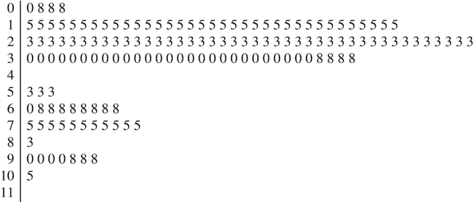

  

  A stem–leaf diagram for the wind directions at Kurume City, Fukuoka, Japan on March 8, 2018 [5]

  Example: Wind Direction Statistics (Rose Diagram)

  Figure 4.4 shows a rose diagram for the data in Table 4.1. As immediately seen, the rose diagram is named for its shape.

  Fig. 4.4

  

  A rose diagram for the data on the wind directions at Kurume City, Fukuoka, Japan. The raw data is given in Table 4.1

• 3. The stem-and-leaf diagram is a histogram retaining the raw data values; in particular, their mode is immediately found from the sample. Each stem, as a column sequence of integers, consists of the data falling in a 10^∘ interval with the leaves being the data values in that interval, sorted in an increasing order. The stem-and-leaf diagram is superior in displaying data without detracting the individual measurements.

  Example: Wind Direction Statistics (Stem–Leaf Diagram)

  Figure 4.3 gives a stem–leaf diagram for the data in Table 4.1. In order to make this diagram, we process the raw data in Table 4.1 by dividing all the numerics by 30^∘. Accordingly, the stem consists of 12 items, and stems 0, 1, 2, 3, … present actual angles 0^∘, 30^∘, 60^∘, 90^∘, …, respectively. Then, for example, leaf 2 | 3 present actual angle 67.5^∘. We remark that this processing of the raw data changes numerics superficially but does not detract intrinsic statistics at all.

• 4. We introduce a kernel density estimation, which is one of nonparametric methods to estimate the distribution for a sample. This method is different from the histograms described above in that the contribution of each data point θ _k is defined as

  $$\displaystyle \begin{aligned}\frac 1{nh} w\Big(\frac{\theta-\theta_k}{h}\Big)d\theta, \end{aligned}$$

  where w(θ) presents a smooth function of θ taking the form of a bump, dθ denotes an infinitely small interval, and h controls the amount of smoothing effect. Then, the kernel density estimation $\hat {f}(\theta )$ is given by the sum of all the contributions:

  $$\displaystyle \begin{aligned}\hat{f}(\theta)d\theta=\frac 1{nh}\sum^n_{k=1}w\Big(\frac{\theta-\theta_k}{h}\Big)d\theta.\end{aligned}$$

  Function w(θ) called the kernel function should be chosen so that its support D, a region where the function takes nonzero values, is small enough for w(θ) to ensure the condition

  $$\displaystyle \begin{aligned}\int_D w(\theta)d\theta=1.\end{aligned}$$

  However, the choice is not crucial to the density estimation but the magnitude of h is because it determines the amount of smoothing effect, namely, the larger h is, the more the density function gets blurred. It is, however, another issue how you determine the value of h.

We note some important points in plotting histograms: Some choice of group boundaries can give rise to a serious distortion of the information about the modal groups observed in the sample; as well, the choice of the bin width should be carefully made so that we can anticipate the shape of the underlying distribution of the sample. It is, however, another issue whether your choice is correct or not.

4.2.3 Summary Statistics

The diagrams described above suggest the existence of the population from which the sample was drawn. Here we introduce basic quantities which describe important features of the sample distribution.

(A) Sample Circular Mean and Sample Circular Standard Deviation

The most popular as well as important statistic is the sample mean, which is ordinarily given by the arithmetic mean:

$$\displaystyle \begin{aligned}\frac 1n\sum^n_{j=1}\theta_j.\end{aligned}$$

Is it correct even for a sample of circular data? No, and it will be obvious if one considers, for example, the sample {10^∘, 350^∘}. We have the arithmetic mean 180^∘, but this cannot be acceptable.

The natural way is to consider that each circular data corresponds to a point located on the unit circle, and thereby the sample of circular data directly transforms into a sample of unit vectors and the sample mean for circular data is to be figured out from the mean vector. The mean vector in terms of vector addition is carried out as

$$\displaystyle \begin{aligned}C=\frac 1n\sum^n_{j=1}\cos \theta_j,\qquad S=\frac 1n\sum^n_{j=1}\sin\theta_j,\qquad R=\sqrt{C^2+S^2},\end{aligned}$$

where R should be chosen to be positive. Then, the mean direction $\bar {\theta }$ of the sample of unit vectors is obtained from

$$\displaystyle \begin{aligned}\cos \bar{\theta}=\frac{C}{R},\qquad \sin \bar{\theta}=\frac{S}{R}.\end{aligned}$$

This mean direction $\bar {\theta }$ corresponds to the mean of the sample of circular data θ _is.

On the other hand, R defined above presents the length of the resultant vector and is no longer a unit vector. R takes the value in the range [0, 1]; if R = 1, it means that all the vectors are in the same direction and hence all data θ _is are coincident. By contrast, R = 0 does not always mean that all the unit vectors distribute in uniformly random directions. A simple counterexample is the sample data {10^∘, 180^∘, 350^∘}. This point will become more clear when we consider statistics for axial data. We hence note that R cannot be a useful measure of deviation.

However, R may present the variance as

$$\displaystyle \begin{aligned}V=1-R\end{aligned}$$

in the case that the sample shows a single modal distribution. We note that circular data is restricted to a finite range and so is the variance. Again, V = 1 does not immediately imply that the sample has a dispersed distribution.

The sample circular standard deviation is also defined as

$$\displaystyle \begin{aligned}v=\sqrt{-2\log (1-V)}.\end{aligned}$$

(We may have other definitions for the standard deviation.) If V  is nearly equal to 1, v can be well approximated by $\sqrt {2V}$.

(B) Advanced Circular Summary Statistics

In order to define advanced statistics, we need some mathematics in complex numbers. From the mean direction $\bar {\theta }$ and the resultant vector length R, we define the first trigonometric moment

$$\displaystyle \begin{aligned}m_1=R(\cos \bar{\theta}+i\sin \bar{\theta}),\end{aligned}$$

where $i=\sqrt {-1}$. In an analogous manner as the mean direction, the pth trigonometric moment is then defined as

$$\displaystyle \begin{aligned}m_p=R_p(C_p+iS_p),\end{aligned}$$

where

$$\displaystyle \begin{aligned}C_p=\frac 1n\sum^n_{i=1}\cos p\theta_i, \qquad S_p=\frac 1n\sum^n_{i=1}\sin p\theta_i,\qquad R_p=\sqrt{C_p^2+S_p^2}.\end{aligned}$$

Note that R ₁ = R.

Using Euler’s formula in complex analysis, $e^{i\theta }=\cos \theta +i \sin \theta$, we have a simple expression:

$$\displaystyle \begin{aligned}C_p+i S_p= \frac 1n \sum^n_{j=1} e^{i p\theta_j}.\end{aligned}$$

Then, we introduce argument μ _p as

$$\displaystyle \begin{aligned}R_p e^{i \mu_p}=\frac 1n \sum^n_{j=1} e^{i p\theta_j}.\end{aligned}$$

In particular, $\mu _1=\bar {\theta }$, but however $\mu _p\ne p\bar {\theta }$ for p ≥ 2 in general.

The centered sample trigonometric moments are also defined as

$$\displaystyle \begin{aligned}m_p^{\prime}=R_p^{\prime}(C_p^{\prime}+i S^{\prime}_p),\end{aligned}$$

where

$$\displaystyle \begin{aligned}C_p^{\prime}=\frac 1n\sum^n_{j=1} \cos p(\theta_j-\bar{\theta}), \qquad S_p^{\prime}=\frac 1n\sum^n_{j=1} \sin p(\theta_j-\bar{\theta}), \end{aligned}$$

and

$$\displaystyle \begin{aligned}R^{\prime}_p=\sqrt{(C_p^{\prime})^2+(S_p^{\prime})^2}.\end{aligned}$$

Since a little calculation leads to $C_1^{\prime }=R$ and $S_1^{\prime }=0$, we have $m_1^{\prime }=R$.

Using Euler’s formula, we have

$$\displaystyle \begin{aligned}R_p^{\prime}e^{i\mu_p^{\prime}}= \frac 1n \sum^n_{j=1} e^{ip(\theta_j-\bar{\theta})} = \frac{e^{-i p\bar{\theta}}}n \sum^n_{j=1} e^{ip\theta_j} = R_p e^{i (\mu_p-p\bar{\theta})},\end{aligned}$$

and therefore $\mu ^{\prime }_p=\mu _p-p\bar {\theta }$, and $R_p^{\prime }=R_p$.

As for a unimodal distribution of the sample, we exploit the first and second centered trigonometric moments, defining advanced statistics: the sample circular dispersion

$$\displaystyle \begin{aligned}\delta =\frac{1-R_2^{\prime}}{2(R^{\prime}_1)^2},\end{aligned}$$

the sample circular skewness

$$\displaystyle \begin{aligned}s=\frac{R_2^{\prime} \sin (\mu_2^{\prime}-2\mu_1^{\prime})}{\sqrt[3]{1-R_1^{\prime}}}, \end{aligned}$$

and the sample circular kurtosis

$$\displaystyle \begin{aligned}k=\frac{R_2^{\prime} \cos (\mu_2^{\prime}-2\mu_1^{\prime})-(R_1^{\prime})^4}{(1-R^{\prime}_1)^2}.\end{aligned}$$

The circular dispersion δ is concerned with confidence interval for the sample mean direction. The skewness s presents the asymmetry of the sample distribution. The kurtosis k presents the peakedness of the sample distribution, and so it is also called peakedness.

Example: Wind Direction Statistics

We have summary quantities for the wind directions given in Table 4.1 as follows: the mean direction $\bar {\theta }=71.7^\circ$, the sample circular variance V = 0.43, and the circular standard deviation v = 1.1. See Figs. 4.2 and 4.4, and verify these results.

4.2.4 Probability Models

Statistical analysis, especially statistical inference, of a sample data is based on the probability of it being obtained. Probability in statistics takes a role in formulating uncertainty of the data, i.e., the data we obtain is drawn from an underlying population. Each sample of the population contains the probability that one will draw it, and we call the set of the probability the probability distribution or distribution simply.

Probability models provide with a distribution for the data a priori. Some probability models have parameters to be inferred from the sample, and other models called nonparametric do not. One usually applies the normal distribution for linear data, then obtaining acceptable results. For circular data, some models appear as a counterpart of the normal distribution for linear data, and the von Mises distribution described below is one of them.

Example: von Mises Distribution

Figure 4.5 shows a von Mises distribution. This distribution is a continuous probability distribution on the circle and was introduced as a circular analogue of the normal distribution. The probability density function is defined by

$$\displaystyle \begin{aligned}f(\theta)=\frac{e^{\kappa \cos{}(\theta-\mu)}}{2\pi I_0(\kappa)}\qquad (0 \leq \theta<2\pi,\ 0\leq \kappa<\infty),\end{aligned}$$

where the parameters μ and 1∕κ correspond, respectively, to the mean value and the variance. We note that the normalization is given by a modified Bessel function I ₀(κ). We have some analytic expressions for the function as

$$\displaystyle \begin{aligned}I_0(\kappa)=\frac 1{2\pi} \int^{2\pi}_0 e^{\kappa \cos{}(\theta-\mu)} d\theta, \end{aligned}$$

and

$$\displaystyle \begin{aligned}I_0(\kappa)=\sum^\infty_{r=0} (r!)^{-2} \left(\frac{\kappa}2\right)^{2r}.\end{aligned}$$

However, these may not be useful for numerical calculation. The use of a software on computer is practical.

Fig. 4.5

The von Mises distribution. We illustrate a von Mises distribution in polar plot; the outer curve presents the value of probability increasing upon the unit circle (the inner curve)

For example, we apply the von Mises distribution to the wind direction data given in Table 4.1. As already calculated above, the circular mean μ = 71.7^∘ and the circular variance 1∕κ = 0.43. Figure 4.6 shows the probability density function in polar plot.

Fig. 4.6

The von Mises distribution applied for the wind direction data given in Table 4.1. Parameters are chosen so that the mean μ = 71.7^∘ and the variance 1∕κ = 0.43. We find that this fits with the rose diagram given in Fig. 4.4. To be precise, we illustrate the graph of polar equation ρ = f(θ) + 1 with μ = 1.25 and the variance κ = 2.33

4.3 Application for Single Cell Movement

In this final section, we apply the circular statistical analysis introduced above for single cell movement. We obtain the sample of a single 3T3 cell in vitro. The 3T3 cell line is a spontaneously immortalized mouse fibroblast cell line established from mouse embryonic tissue.

Figure 4.7 shows the sample trajectory of a single 3T3 cell moving on a dish freely. We plot the data points by time lapse imaging of the cell movement and then connect them with line segments in time sequence.

Fig. 4.7

The sample of a single 3T3 cell moving freely on a dish

Figure 4.8 shows the directions of motion obtained from the sample trajectory in both circular histogram and rose diagram. From the data, we have the mean circular mean direction 121^∘ and the circular variance 0.93. Since the circular variance takes a value in between 0 and 1 and the greater it is the more random (irregular) the movement is, we consider from the present result that the 3T3 cell chooses the direction of movement with almost equal probability (Fig. 4.9).

Fig. 4.8

The directions of motion obtained from the sample trajectory

Fig. 4.9

The mean squared displacement for the sample trajectory

Furthermore, we calculate the mean squared displacement from the sample trajectory data, so we test that the movement observed is a random walk or not. We use a log–log plot for the figure, and hence the line of the linear minimum mean squared error estimator gives the exponent λ for the MSD with respect to time: MSD ∝ t ^λ. The slope of the line is read as 1.0, i.e. λ = 1.0, and accordingly the result suggests that the present cell movement should be considered as diffusive. Hence we conclude from the sample data given in Fig. 4.7 that the 3T3 cell moves as a random walk.

We finally make a remark on the calculation of the MSD from the sample data before closing the chapter. From a sample trajectory containing N + 1 points of position (x(t), y(t)) at time t, we actually compute the MSD as

$$\displaystyle \begin{aligned} \begin{array}{rcl} \mbox{MSD}(\tau)& =&\displaystyle \langle (x(t+\tau)-x(t))^2+ (y(t+\tau)-y(t))^2 \rangle \\ & =&\displaystyle \frac 1{N-n+1} \sum^{N-n}_{i=0} \left[ ( x( (i+n)\varDelta t )-x( i \varDelta t ) )^2 \right. \\ & &\displaystyle \left. + ( y( (i+n)\varDelta t )-y(i \varDelta t) )^2 \right], \end{array} \end{aligned} $$

(4.5)

where τ = nΔt (n = 0, 1, 2, …, N).

References

D. Campos, Méndez, V., Llopis, I.: Persistent random motion: uncovering cell migration dynamics. J. Theor. Biol. 267, 526–534 (2010)
Dieterich, P., Klages, R., Preuss, R., Schwab, A.: Anomalous dynamics of cell migration. Natl. Acad. Sci. 105, 459–463 (2008)
Fürth, R.: Die brownsche bewegung bei berücksichtigung einer persistenz der bewegungsrichtung. mit anvendungen auf die bewegung lebender infusorien [in German]. Z. Phys. 2, 244—256 (1920)
Gorelik, R., Gautreau, A.: Quantitative and unbiased analysis of directional persistence in cell migration. Nat. Protocols 9, 1931–1943 (2014)
The Japan meteological agency data service website: https://www.jma.go.jp/jma/menu/menureport.html. (in Japanese)
Masuzzo, P., Troys, M.V., Ampe, C., Martens, L.: Taking aim at moving targets in computational cell migration. Trends Cell Biol. 26, 88–110 (2016)
Peruani, F., Morelli, L.G.: Self-propelled particles with fluctuating speed and direction of motion in two dimension. Phys. Rev. Lett. 99, 010602 (2007)
Selmeczi, D., Li, L., Pedersen, L., Nrrelykke, S.F., Hagedorn, P.H., Mosler, S., Larsen, N.B., Cox, E.C., Flyvbjerg, H.: Cell motility as random motion: a review. Eur. Phys. J. Topics 157, 1–15 (2008)
Wu, P.H., Giri, A., Wirtz, D.: Statistical analysis of cell migration in 3d using the anisotropic persistent random walk model. Nat. Protocols 10, 517–525 (2015)
Author information
Authors and Affiliations
Corresponding author
Editor information
Editors and Affiliations
Rights and permissions
Copyright information
© 2021 Springer Nature Singapore Pte Ltd.
About this chapter
Cite this chapter
Kanai, M., Tonami, K., Tozawa, H. (2021). Statistical Analysis of Cellular Directional Movement: Application for Research of Single Cell Movement. In: Tokihiro, T. (eds) Mathematical Modeling for Genes to Collective Cell Dynamics. Theoretical Biology. Springer, Singapore. https://doi.org/10.1007/978-981-16-7132-6_4
Download citation
DOI: https://doi.org/10.1007/978-981-16-7132-6_4
Published:
Publisher Name: Springer, Singapore
Print ISBN: 978-981-16-7131-9
Online ISBN: 978-981-16-7132-6
eBook Packages: Mathematics and StatisticsMathematics and Statistics (R0)