Applications of Engineering Mathematics in Real Life Civil Engineering: Practical Examples

Abstract

Mathematics is part of our day-to-day life. Many field works employ extensive use of mathematics knowingly or unknowingly. Engineering field cannot be imagined without involvement of mathematics, and it forms the backbone of mother branch ‘civil engineering.’ For many peoples, applying mathematics to engineering problems found a little difficult. The reason behind this, in most of cases, civil engineering problems are not discussed with respect to their compatibility with basic mathematics which makes difficult for people to understand interlinking. The aim of this paper is to exhibit some applications of mathematics to various fields of civil engineering. Some simple and basic examples are discussed to build a bridge between civil engineering and engineering mathematics. This paper is divided into three case studies. Each case study represents application mathematics with examples in particular field of civil engineering.

1 Introduction

Mathematics is part of our day-to-day life. Many field works employ extensive use of mathematics knowingly or unknowingly [1]. Engineering field cannot be imagined without involvement of mathematics, and it forms the backbone of mother branch ‘civil engineering.’ Engineering mechanics, essential part of civil engineering, is the extension of various applications of mathematics along with physics [2]. Research and development in the field of civil engineering cannot be imagine without mathematics [3]. Matrices, linear algebra, differential equations, integration (double and triple integration) numerical analysis calculus, statistics, probability are taught as they are essential to realize numerous civil engineering fields such as structural engineering, fluid mechanics, water resource engineering, geotechnical engineering, foundation engineering, environmental engineering and transportation engineering to name a few. However, it becomes necessary to correlate basic mathematics to its real life applications of civil engineering [4]. The theory of matrices can be implemented to structural analysis to perform stability checks [5]. Similarly, differential equations are used to solve complex networks involved in fluid mechanics as well as structural analysis [6]. Concepts of probability and statistics have direct application in water resource engineering [4].

For many peoples, applying mathematics to engineering problems found a little difficult. The reason behind this, in most of cases, civil engineering problems are not discussed with respect to their compatibility with basic mathematics which makes difficult for people to understand interlinking [3]. The aim of this paper is to exhibit some applications of mathematics to various fields of civil engineering. Some simple and basic examples are discussed to build a bridge between civil engineering and engineering mathematics. This paper is divided into three case studies. Each case study represents application mathematics with examples in particular field of civil engineering.

2 Case Studies

Mathematics is widely used in many real life problems associated civil engineering. Few applications of engineering mathematics various fields of civil engineering are explained in subsequent paragraph.

2.1 Water Resources Engineering

Data availability and data consistency are of utmost importance in water resources engineering [7]. Statistics and probability help in analysis of data and checking the quality of available data. Many hydraulic engineering applications concerned with rainfall events and floods requires the estimation of probability of occurrence of a particular event. Frequency analysis of such events provides useful information regarding the rainfall/runoff data. The probability of occurrence of an event is studied using frequency analysis of annual data series of rainfall. The occurrence probability of an event is denoted by ‘P,’ while, the non-occurrence probability of the same event is given by q = (1 − P). The recurrence interval (return period) is given by Eq. 1. Then, occurrence probability of the event ‘r’ times in ‘n’ successive years ‘P(r, n)’ is given by the binomial distribution as represented by Eq. 2.

$$T = \frac{1}{P}{ }$$

(1)

$$P_{r,n} = { }^{n} C_{r} P_{r} q^{n - r} = { }\frac{n!}{{\left( {n - r} \right)!r!}}P^{r} q^{n - r} { }$$

(2)

2.2 Structural Engineering

Use of mathematical equations to find solutions of various problems related to structural design is a traditional practice used by man-kinds from ages. For example, curve fitting can be used to formulate graphical relationship between two parameters to form the basic lows (laws of load vs. deflection, load vs. effort, etc.) is common practice [8]. Similarly, the differentiation and integration methods are primarily used in analysis of determinate as well as indeterminate structures. Matrices have distinguished application in stiffness method and flexibility method (matrix method of structural analysis) of structural analysis [9]. Stiffness is defined as the action required at the simply supported end of the member to cause a unit displacement, whereas the flexibility is the displacement produced due to application of unit force on the member.

2.3 Stiffness Matrix

Stiffness equation in the matrix form can be written as:

$$\Delta = k^{ - 1} \left[ {P - P^{\prime } } \right]$$

(3)

$$\left[ {\begin{array}{*{20}c} {\Delta_{1} } \\ {\Delta_{2} } \\ {\Delta_{3} } \\ \end{array} } \right] = k^{ - 1} \left\{ {\left[ {\begin{array}{*{20}c} {P_{1} } \\ {P_{2} } \\ {P_{3} } \\ \end{array} } \right] - \left[ {\begin{array}{*{20}c} {P_{1}^{\prime } } \\ {P_{2}^{\prime } } \\ {P_{3}^{\prime } } \\ \end{array} } \right]} \right\}$$

(4)

where,

∆₁:

Slope or deflection at co-ordinate 1.

∆₂:

Slope or deflection at co-ordinate 2.

∆₃:

Slope or deflection at co-ordinate 3.

P₁:

External Slope or external moment at co-ordinate 1.

P₂:

External Slope or external moment at co-ordinate 2.

P₃:

External Slope or external moment at co-ordinate 3.

$P_{1}^{\prime }$:

Fixed end moment at co-ordinate 1.

$P_{2}^{\prime }$:

Fixed end moment at co-ordinate 2.

$P_{3}^{\prime }$:

Fixed end moment at co-ordinate 3.

2.4 Application of Integration and Differential Equations

Macaulay's method used for estimating the slope and deflections in a beam uses integration and differential equations, represents wide application of mathematics in civil (structural) engineering [10]. Equation 5 represents the differential equation of elastic curve, the ‘EI’ is known as flexural rigidity of beam. By integrating the differential equation of elastic curve, we get slope of the beam (Eq. 6). Whereas deflection of beam (Eq. 7) is be obtained by integrating the slope Eq. 6.

$${\text{EI}} \frac{{{\text{d}}_{y}^{2} }}{{{\text{d}}x^{2} }} = M$$

(5)

$${\text{EI}} \frac{{{\text{d}}y}}{{{\text{d}}x}} = \smallint M\,{\text{d}}x + C_{1}$$

(6)

$${\text{EI}}\,y = \smallint \smallint M\,{\text{d}}x + C_{1} x + C_{2} a$$

(7)

2.5 Fluid Mechanics

Mathematics has wide applications in fluid mechanics branch of civil engineering. The simple application of ordinary differential equations in fluid mechanics is to calculate the viscosity of fluids [11]. Viscosity is the property of fluid which moderate the movement of adjacent fluid layers over one another [4]. Figure 1 shows cross section of a fluid layer. Consider two fluid layers ‘dy’ distance apart moving with velocities ‘u’ and ‘u + du,’ respectively. The movement of fluid layers will produce in shear stress ‘τ’ on the contact surface. This shear stress is proportional to the rate of change of velocity with respect to ‘y’ and is given by Eq. 8.

Fig. 1

Fluid profile

$$\tau { } \propto { }\frac{{{\text{d}}u}}{{{\text{d}}y}}\quad {\text{Therefore}}, = \mu \frac{{{\text{d}}u}}{{{\text{d}}y}}$$

(8)

where, ‘µ’ is constant of proportionality.

2.6 Applications of Bernoulli’s Differential Equations

The Bernoulli’s Differential Equations is most commonly used application of mathematics in fluid mechanics branch of civil engineering [4]. The Bernoulli’s Differential Equations are used to calculate the head loss in pipe flows under different conditions [12]. For instance, due to sudden enlargement of pipe the fluid flow will lose its energy. Consider two sections as shown in Fig. 2. The Bernoulli’s Equation (Eq. 9) can be applied between the two sections. Solving Eq. 9, the head loss due to sudden enlargement can be estimated as shown in Eq. 10.

Fig. 2

Sudden enlargement of pipe

$$\frac{{P_{1} }}{\rho g} + \frac{{v_{1}^{2} }}{2g} + Z_{1} = \frac{{P_{2} }}{\rho g} + \frac{{v_{2}^{2} }}{2g} + Z_{2} + h_{e}$$

(9)

where h_e = head loss due to sudden enlargement.

$Z_{1} = Z_{2}$…For Horizontal Pipe.

$$\frac{{P_{1} }}{\rho g} + \frac{{v_{1}^{2} }}{2g} = \frac{{P_{2} }}{\rho g} + \frac{{v_{2}^{2} }}{2g} + h_{e}$$

$$h_{e} = \left( {\frac{{P_{1} }}{\rho g} - \frac{{P_{2} }}{\rho g}} \right) + \left( {\frac{{v_{1}^{2} }}{2g} - \frac{{v_{2}^{2} }}{2g}} \right)$$

(10)

2.7 Applications of Vector, Scalar, Continuity Equation, Laplace Equation and Partial Derivative

Vector, Scalar, Continuity Equation, Laplace Equation, and Partial Derivative are basic forms of mathematical equations widely used to explain many physical phenomenon’s [6]. A common example elaborating use of all these applications of mathematics together is explained using velocity potential function (Ø) and stream function ($\varphi$).

2.8 Velocity Potential Function (Ø)

Velocity potential function is function of space and time. It is denoted by ‘Ø.’ Velocity of fluid in any direction can be obtained by negative partial differentiation of velocity potential function with respect to that direction.

By mathematical expression we can write, Ø = f(x, y, z).

$$u = - \frac{\partial \emptyset }{{\partial x}}, v = - \frac{\partial \emptyset }{{\partial y}}, w = - \frac{\partial \emptyset }{{\partial z}}$$

(11)

where u is component of velocity in x direction, v is component of velocity in y direction, w is component of velocity in z direction.

For incompressible fluid, continuity equation of steady flow is (Eq. 12).

$$\frac{\partial u}{{\partial x}} + \frac{\partial v}{{\partial y}} + \frac{\partial w}{{\partial z}} = 0$$

(12)

After substitution of u, v and w from Eqs. 1 in 2, we get:

$$\frac{\partial }{\partial x}\left( { - \frac{\partial \emptyset }{{\partial x}}} \right) + \frac{\partial }{\partial y}\left( { - \frac{\partial \emptyset }{{\partial y}}} \right) + \frac{\partial }{\partial z}\left( { - \frac{\partial \emptyset }{{\partial z}}} \right) = 0$$

Therefore,

$$\frac{{\partial^{2} \emptyset }}{{\partial x^{2} }} + \frac{{\partial^{2} \emptyset }}{{\partial y^{2} }} + \frac{{\partial^{2} \emptyset }}{{\partial z^{2} }} = 0$$

(13)

This (Eq. 13) is known as Laplace equation.

2.9 Stream Function ($\boldsymbol{\varphi }$)

Stream function is scalar function. Velocity perpendicular to any direction can be obtained by partial differentiation of stream function with respect to that direction [6]. For instance, $\varphi = f \left( {x,y} \right)$,

$$u = - \frac{\partial \varphi }{{\partial y}}, v = \frac{\partial \varphi }{{\partial x}}$$

(14)

The continuity equation for 2-D flow:

$$\frac{\partial u}{{\partial x}} + \frac{\partial v}{{\partial y}} = 0$$

(15)

From Eqs. 4 in 5, we get:

$$\frac{\partial }{\partial x}\left( { - \frac{\partial \varphi }{{\partial y}}} \right) + \frac{\partial }{\partial y}\left( {\frac{\partial \varphi }{{\partial x}}} \right) = 0$$

$$- \frac{{\partial^{2} \varphi }}{\partial x\partial y} + \frac{{\partial^{2} \varphi }}{\partial x\partial y} = 0$$

(16)

Equation 16 is known as Laplace equation. Any equation satisfying the Laplace equation shows the possible case of fluid flow.

3 Examples

Applications of mathematics in civil engineering as explained in back forth paragraphs. Few crucial application based examples are as follows.

• 1. Maximum one day rainfall for 50 years return interval in Delhi is found to be 280 mm. what is the possibility of one day rainfall more than 280 mm depth

• (i) One time in 20 consecutive years,

• (ii) Twice in 15 consecutive years,

• (iii) At least once in 20 consecutive years.

Solution

Here,

$$\begin{aligned} P & = \frac{1}{T} = \frac{1}{50}{ } = 0.02 \\ q & = (1 - P) = (1 - 0.02) = {\mathbf{0}}{\mathbf{.98}} \\ \end{aligned}$$

Case (i): n = 20, r = 1

$$\begin{aligned} P_{1,20} & = \frac{20!}{{\left( {20 - 1} \right)!1!}}P^{1} q^{20 - 1} \\ P_{1,20} & = \frac{20!}{{19!1!}}\left( {0.02} \right)^{1} \left( {0.98} \right)^{20 - 1} = 20 \times \left( {0.98} \right)\left( {0.98} \right)^{19} \\ P_{1,20} & = 20 \times 0.02 \times 0.68123 = 0.272 \\ \end{aligned}$$

Case (ii): n = 15, r = 2

$$\begin{aligned} P_{2,15} & = \frac{15!}{{\left( {15 - 2} \right)!2!}}\left( {0.02} \right)^{2} \left( {0.98} \right)^{15 - 2} \\ P_{2,15} & = \frac{15!}{{13!2!}}\left( {0.02} \right)^{2} \left( {0.98} \right)^{13} = 15 \times \frac{14}{2} \times 0.0004 \times 0.769 \\ P_{2,15} & = 0.323 \\ \end{aligned}$$

Case (iii): n = 20

$$\begin{aligned} P_{1} & = 1 - q^{n} = 1 - \left( {1 - P} \right)^{n} \\ P_{1} & = 1 - \left( {1 - 0.02} \right)^{20} = 0.332 \\ \end{aligned}$$

• 2. A river catchment consists of four rain-gauges with average yearly rainfall of 800, 620, 400, and 540 mm.

• (i) The optimal rain-gauge stations required to limit the error up to 10%.

• (ii) Calculate the extra rain-gauges required.

Solution

Mean annual average precipitation

$$\overline{P} = \frac{\sum P}{n} = \frac{{\left( {800 + 620 + 400 + 540} \right)}}{4} = {\mathbf{590}}\,{\text{mm}}$$

Mean of squares

$$\overline{{P^{2} }} = \frac{{\sum P^{2} }}{n} = \frac{{\left( {800^{2} + 620^{2} + 400^{2} + 540^{2} } \right)}}{4} = {\mathbf{369,000}}$$

Sample Standard Deviation

$$\begin{aligned} \sigma & = \sqrt {\frac{n}{n - 1}\left[ {\overline{{P^{2} }} - \left( {\overline{P}} \right)^{2} } \right]} \\ \sigma & = \sqrt {\frac{4}{4 - 1}\left[ {369000 - \left( {590} \right)^{2} } \right]} \\ \sigma & = {\mathbf{166}}{\mathbf{.93}} \\ \end{aligned}$$

Calculation of coefficient of variation of the rainfall

$$\begin{aligned} C_{v} & = \frac{100 \sigma }{{\overline{P}}} \\ C_{v} & = \frac{100 \times 166.93}{{590}} \\ C_{v} & = {\mathbf{28}}{\mathbf{.29}} \\ \end{aligned}$$

Optimum number of rain-gauges (N) are calculated using following equations:

$$\begin{aligned} N & = \left( {\frac{{C_{v} }}{E}} \right)^{2} \\ N & = \left( {\frac{28.29}{{10}}} \right)^{2} = 8.004 \approx 8 \\ \end{aligned}$$

Additional gauges required = 8-Existing gauges (4) = 4 Numbers.

• 3. Simply supported beam carries a concentrated load ‘P’ at its middle point. Corresponding to various values of ‘P,’ maximum deflection is tabulated as below. Find law in the form $Y=ap+b$ using least square method, (where, ‘a’ and ‘b’ are constants) (Table 1).

  Table 1 Load and distribution table

P	100	120	140	160	180	200
Y	0.90	1.10	1.20	1.40	1.60	1.70

Solution

We have,

$$Y = ap + b$$

(17)

The normal equations are given as:

$$\sum Y = a\sum p + nb{ }$$

(18)

$$\sum pY = a\sum p^{2} + b\sum p{ }$$

(19)

From Eq. 18,

$$7.9 = 900a + 6b{ }$$

(20)

From Eq. 19,

$$1242 = 142,000a + 900b{ }$$

(21)

Solving Eqs. 20 and 21

$$a = 8.14 \times 10^{ - 3} \quad {\text{and}}\quad b = 0.095$$

Therefore, Eq. 17, can be written as:

$$Y = \left( {8.14 \times 10^{ - 3} } \right){ }p + 0.095{ }$$

• 4. Analyze the continuous beam as shown in Fig. 3.

  Fig. 3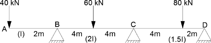

  

  Point load on continuous beam

Solution

Slope at point B, C and D, i.e., $\theta_{B } ,\theta_{C} , \theta_{D}$ can be calculated by using Stiffness Equation

$$\Delta = k^{ - 1} \left[ {P - P^{\prime}} \right]$$

$$\left[ {\begin{array}{*{20}c} {\Delta_{1} } \\ {\Delta_{2} } \\ {\Delta_{3} } \\ \end{array} } \right] = k^{ - 1} \left\{ {\left[ {\begin{array}{*{20}c} {P_{1} } \\ {P_{2} } \\ {P_{3} } \\ \end{array} } \right] - \left[ {\begin{array}{*{20}c} {P_{1}^{^{\prime}} } \\ {P_{2}^{^{\prime}} } \\ {P_{3}^{^{\prime}} } \\ \end{array} } \right]} \right\}$$

where

$$\begin{aligned} \Delta_{1} & = \theta_{B} ,\Delta_{2} = \theta_{C} ,\Delta_{3} = \theta_{D} \\ P_{1} & = - 80\,{\text{kN}}\,{\text{m}}, P_{2} = 0, P_{3} = 0 \\ P_{1}^{\prime } & = - 60\,{\text{kN}}\,{\text{m}},P_{2}^{\prime } = 24.44\,{\text{kN}}\,{\text{m}},P_{3}^{\prime } = 71.11\,{\text{kN}}.{\text{m}} \\ \end{aligned}$$

$$\left[ {\begin{array}{*{20}c} {\theta_{B } } \\ {\theta_{C} } \\ {\theta_{D} } \\ \end{array} } \right] = k^{ - 1} \left\{ {\left[ {\begin{array}{*{20}c} { - 80} \\ 0 \\ 0 \\ \end{array} } \right] - \left[ {\begin{array}{*{20}c} {60} \\ {24.44} \\ {71.11} \\ \end{array} } \right]} \right\}$$

where,

$$K^{ - 1} = \frac{1}{{1.5\,{\text{EI}}}}\left[ {\begin{array}{*{20}l} {1.75} \hfill & { - 0.5} \hfill & {0.25} \hfill \\ { - 0.5} \hfill & 1 \hfill & { - 0.5} \hfill \\ {0.25} \hfill & { - 0.5} \hfill & {1.75} \hfill \\ \end{array} } \right]$$

Solving matrix, we get

$$\theta_{B } = \frac{ - 27.038}{{{\text{EI}}}},\theta_{C } = \frac{14.077}{{{\text{EI}}}}\quad {\text{and}}\quad \theta_{C } = \frac{ - 78.15}{{{\text{EI}}}}$$

• 5. For given simply supported beam subjected to point load at center find slope at support and deflection at the mid span of beam (Fig. 4) [5].

  Fig. 4

  

  Point load acting at the center

Let us consider FBD of the beam (Fig. 5).

Fig. 5

Free body diagram of beam

Solution

Differential equation of elastic curve of beam is given by

$${\text{EI}} \frac{{{\text{d}}^{2} y}}{{{\text{d}}x^{2} }} = M = \frac{W}{2} \times X\quad \quad \quad\quad\quad\quad\quad\quad\quad\quad\quad\quad\quad \left( {\text{i}} \right)$$

By integrating above Eq. (i) we get slope of the beam:

$${\text{EI}} \frac{{{\text{d}}y}}{{{\text{d}}x}} = \frac{W}{2} \times \frac{{X^{2} }}{2} + C_{1} = \frac{{WX^{2} }}{4} + C_{1} \quad \quad \quad\quad\quad \left( {{\text{ii}}} \right)$$

Again integrating equation to (ii) we get,

$${\text{EI}}.y = \frac{{WX^{3} }}{12} + C_{1} X + C_{2} \quad \quad \quad\quad\quad\quad\quad\quad\quad\quad\quad \left( {{\text{iia}}} \right)$$

At point at center of beam, $X = \frac{L}{2}$ and $\frac{{{\text{d}}y}}{{{\text{d}}x}} = 0$. Applying Eq. (ii), we get:

$${\text{EI}} \left( 0 \right) = \frac{W}{4} \times \frac{{L^{2} }}{4} + C_{1}$$

Therefore,

$$C_{1} = \frac{{ - WL^{2} }}{16}\quad \quad \quad\quad\quad\quad\quad\quad\quad\quad\quad\quad\quad\quad\quad\quad\quad\quad \left( {{\text{iii}}} \right)$$

Put $C_{1}$ in Eq. (ii)

$${\text{EI}} \frac{{{\text{d}}y}}{{{\text{d}}x}} = \frac{{WX^{2} }}{4} + \frac{{ - WL^{2} }}{16}\quad \quad \quad \quad\quad\quad\quad\quad\quad\quad\quad\quad\left( {{\text{iv}}} \right)$$

At point A, X = 0, Therefore,

$$\begin{aligned} {\text{EI}} \frac{{{\text{d}}y}}{{{\text{d}}x}} & = \frac{{ - WL^{2} }}{16} \\ \left( { \frac{{{\text{d}}y}}{{{\text{d}}x}}} \right)_{A} & = \frac{{ - WL^{2} }}{{16\,{\text{EI}}}} \\ \end{aligned}$$

Therefore,

Clockwise rotation.

By symmetry

Clockwise rotation.

Let us consider Eq. (iia)

$${\text{EI}}.y = \frac{{WX^{3} }}{12} + C_{1} X + C_{2} \quad \quad \quad\quad\quad\quad\quad\quad\quad\quad \left( {{\text{iia}}} \right)$$

At point A X = 0, Y = 0, we get C₂ = 0 and we have $C_{1} = \frac{{ - WL^{2} }}{16}$.

Therefore,

$${\text{EI}}.y = \frac{{WX^{3} }}{12} - \frac{{WL^{2} }}{16}\quad \quad \quad\quad\quad\quad\quad\quad \left( {\text{v}} \right)$$

At point C, X = L/2.

Put in Eq. (v), we get

$${\text{EI}}.y = \frac{{WL^{3} }}{48}\quad \quad \quad\quad\quad\quad\quad\quad\quad\quad\quad\quad \left( {{\text{vi}}} \right)$$

Deflection at the center of simply supported beam

$$y = \frac{{WL^{3} }}{{48\,{\text{EI}}}}\quad \quad \quad\quad\quad\quad\quad\quad\quad\quad\quad\quad\quad\quad \left( {{\text{vii}}} \right)$$

• 6. Calculate slope at the support and deflection at the center of simply supported beam of span 10 m subjected to point load of 50 kN at the center of the span [13]. Take EI = 31,300 kN m²

Solution

See Fig. 6.

Fig. 6

Point load of 50 kN at the center of the span

$$\begin{aligned} \theta_{A} & = \theta_{B} = \frac{{WL^{2} }}{{16\,{\text{EI}}}} \\ \theta_{A} = \theta_{B} & = \frac{{50 \times 10^{2} }}{16 \times 31,300} = 9.984 \times 10^{ - 3} \,{\text{Radian}} \\ & = 9.984 \times 10^{ - 3} \times \frac{180}{\pi } = 0.572^{0} \\ \delta_{C} & = \frac{{WL^{3} }}{{48\,{\text{EI}}}} = \frac{{50 \times 10^{3} }}{48 \times 31300 } = 0.0333\,{\text{m}} = 33.28\,{\text{mm}} \\ \end{aligned}$$

• 7. For given cantilever beam subjected to point load at end find slope and deflection at the end span of beam.

Solution

Let’s consider reaction at a distance ‘x’ as shown in Figs. 7 and 8.

Fig. 7

Cantilever beam subjected to point load

Fig. 8

Free body diagram Cantilever beam subjected to point load

Using Eq. (i),

$${\text{EI}} \frac{{{\text{d}}^{2} y}}{{{\text{d}}x^{2} }} = M = Wx - WL\quad \quad \quad\quad\quad\quad\quad\quad\quad \left( {\text{i}} \right)$$

On integrating,

$${\text{EI}} \frac{{{\text{d}}y}}{{{\text{d}}x}} = \frac{{W.x^{2} }}{2} - WLx + C_{1} \quad \quad \quad\quad\quad\quad\quad\quad \left( {{\text{ii}}} \right)$$

Again integrating,

$${\text{EI}}.y = \frac{{W.x^{3} }}{6} - \frac{{WLx^{2} }}{2} + C_{1} .x + C_{2} \quad \quad \quad\quad \left( {{\text{iii}}} \right)$$

Consider boundary conditions, x = 0, $\frac{{{\text{d}}y}}{{{\text{d}}x}} = 0$.

Substituting in Eq. (ii), we get

$$C_{1} = 0$$

Substituting in Eq. (iii), we get

$$C_{2} = 0$$

Therefore, Eqs. (ii) and (iii) can be written as:

$${\text{EI }}\frac{{{\text{d}}y}}{{{\text{d}}x}} = \frac{{W.x^{2} }}{2} - WLx\quad \quad \quad\quad\quad\quad\quad\quad\quad \left( {{\text{iv}}} \right)$$

$${\text{EI}}.y = \frac{{W.x^{3} }}{6} - \frac{{WLx^{2} }}{2}\quad \quad \quad\quad\quad\quad\quad\quad\quad \left( {\text{v}} \right)$$

Put x = L en in Eq. (iv) to calculate slope at free end of beam.

Therefore,

$${\text{EI}} \frac{{{\text{d}}y}}{{{\text{d}}x}} = \frac{{W.x^{2} }}{2} - WLx\quad \quad \quad\quad\quad\quad\quad\quad\quad \left( {{\text{iv}}} \right)$$

$${\text{EI}} \frac{{{\text{d}}y}}{{{\text{d}}x}} = \frac{{W.L^{2} }}{2} - W.L.L$$

$${\text{EI}} \frac{{{\text{d}}y}}{{{\text{d}}x}} = \frac{{W.L^{2} }}{2} - WL^{2}$$

$$\frac{{{\text{d}}y}}{{{\text{d}}x}} = - \frac{{W.L^{2} }}{{2\,{\text{EI}}}} = \theta \quad \quad \quad\quad\quad\quad\quad\quad\quad\quad\quad \left( {{\text{vi}}} \right)$$

Put x = L en in Eq. (v) to calculate deflection at free end of beam.

Therefore,

$${\text{EI}}.y = \frac{{W.x^{3} }}{6} - \frac{{WLx^{2} }}{2}\quad \quad \quad\quad\quad\quad\quad\quad\quad \left( {\text{v}} \right)$$

$${\text{EI}}.y = \frac{{W.L^{3} }}{6} - \frac{{W.L.L^{2} }}{2}$$

$$y = \frac{{W.L^{3} }}{{3\,{\text{EI}}}}$$

• 8. For given cantilever beam subjected to point load at end find slope and deflection at the end span of beam.

  $$\begin{aligned} {\text{Slope:}}\,\theta_{B} & = \frac{{W.L^{2} }}{{2\,{\text{EI}}}} = \frac{2500}{{{\text{EI}}}} , \\ {\text{Deflection:}}\,Y_{B} & = \frac{{W.L^{3} }}{{3\,{\text{EI}}}} = \frac{16666.67}{{{\text{EI}}}} \\ \end{aligned}$$

• 9. The discharge through a level pipe is 0.25 m³/s. The pipe diameter is 0.2 m and suddenly enlarged to 0.4 m so that the intensity of pressure reduced to 11.772 N/cm². If $h_{e} = 1.816m.$ Estimate the intensity of pressure in large pipe.

Solution

$$Q = 0.25{ }\,{\text{m}}^{3} /{\text{s}}.{ }$$

Diameter of small pipe, $D_{1} = 200{ }\,{\text{mm}} = 0.20\,{\text{m}}$

$$\begin{aligned} {\text{Area}}\,A_{1} & = { }\frac{\pi }{4}{ }D_{1}^{2} = { }\frac{\pi }{4}{ }0.2^{2} = 0.03141{ }\,{\text{m}}^{2} \\ D_{2} & = 400{ }\,{\text{mm}} = 0.4\,{\text{m}} \\ { }A_{2} & = { }\frac{\pi }{4}{ }D_{2}^{2} = { }\frac{\pi }{4}{ }0.4^{2} = 0.12564\,{\text{m}}^{2} \\ Q & = 250{ }\,{\text{L}}/{\text{s}} = 0.25{ }\,{\text{m}}^{3} /{\text{s}} \\ V_{1} & = { }\frac{Q}{{A_{1} }} = { }\frac{0.25}{{0.03141}} = 7.96{ }\,{\text{m}}/{\text{s}} \\ V_{2} & = { }\frac{Q}{{A_{2} }} = { }\frac{0.25}{{0.12564}} = 1.99\,{\text{m}}/{\text{s }} \\ P_{1} & = 11.772\,\frac{{\text{N}}}{{{\text{cm}}^{2} }} = 11.772 \times { }10^{4} \,{ }\frac{{\text{N}}}{{{\text{m}}^{2} }}{ } \\ \end{aligned}$$

Loss of head due to enlargement = $h_{e} = 1.816m$

$$\frac{{P_{1} }}{\rho g} + \frac{{v_{1}^{2} }}{2g} + Z_{1} { } = { }\frac{{P_{2} }}{\rho g} + \frac{{v_{2}^{2} }}{2g} + Z_{2} + h_{e}$$

$Z_{1}$ = $Z_{2}$…For Horizontal Pipe.

$$\begin{aligned} \frac{{11.772 \times { }10^{4} }}{1000 \times 9.81} + \frac{{7.96^{2} }}{2 \times 9.81}{ } & = { }\frac{{P_{2} }}{1000 \times 9.81} + \frac{{1.99^{2} }}{2 \times 9.81} + 1.816 \\ P_{2} & = 12.96{ } \times { }10^{4} { }\frac{{\text{N}}}{{{\text{m}}^{2} }}{ } \\ \end{aligned}$$

• 10. The velocity potential function $\left( \emptyset \right)$ is given by an expression:

  $$\emptyset = - \frac{{xy^{3} }}{3} - x^{2} + \frac{{x^{3} y}}{3} + y^{2}$$

Find: (1) velocity components in x and y directions. (2) Show that $\emptyset$ represents a possible case of flow.

Solution

Given

$$\emptyset = - \frac{{xy^{3} }}{3} - x^{2} + \frac{{x^{3} y}}{3} + y^{2}$$

The partial derivatives of $\emptyset$ w.r.t. x and y are

$$\begin{aligned} \frac{\partial \emptyset }{{\partial x}} & = - \frac{{y^{3} }}{3} - 2x + \frac{{3x^{2} y}}{3} \\ \frac{\partial \emptyset }{{\partial y}} & = - \frac{{3xy^{2} }}{3} + \frac{{x^{3} }}{3} + 2y \\ \end{aligned}$$

We know that

$$u = - \frac{\partial \emptyset }{{\partial y}} = - \left( { - \frac{{y^{3} }}{3} - 2x + \frac{{3x^{2} }}{3}} \right)$$

$$u = \frac{{y^{3} }}{3} + 2x - x^{2} y\quad \quad \quad\quad\quad\quad\quad\quad\quad\quad\quad\quad\quad\quad\quad\quad\quad ({\text{i}})$$

$$v = - \frac{\partial \emptyset }{{\partial x}} = - \left( { - \frac{{3xy^{2} }}{3} + \frac{{x^{3} }}{3} + 2y} \right)$$

$$v = xy^{2} - \frac{{x^{3} }}{3} - 2y\quad \quad \quad\quad\quad\quad\quad\quad\quad\quad\quad\quad\quad\quad\quad\quad\quad ({\text{ii}})$$

$\emptyset$ Must satisfy Laplace equation for the possible case of fluid flow.

Laplace equation for two-dimensional flow:

$$\frac{{\partial^{2} \emptyset }}{{\partial x^{2} }} + \frac{{\partial^{2} \emptyset }}{{\partial y^{2} }} = 0\quad \quad \quad\quad\quad\quad\quad\quad\quad\quad\quad\quad\quad\quad\quad\quad\quad\quad\quad \left( {{\text{iii}}} \right)$$

$$\frac{\partial \emptyset }{{\partial x}} = - \frac{{y^{3} }}{3} - 2x + x^{2} y$$

Therefore,

$$\frac{{\partial^{2} \emptyset }}{{\partial x^{2} }} = - 2 + 2xy\quad \quad \quad\quad\quad\quad\quad\quad\quad\quad\quad\quad\quad\quad\quad\quad\quad\quad ({\text{iv}})$$

$$\frac{\partial \emptyset }{{\partial y}} = - xy^{2} + \frac{{x^{3} }}{3} + 2y$$

$$\frac{{\partial^{2} \emptyset }}{{\partial y^{2} }} = - 2xy + 2\quad \quad \quad\quad\quad\quad\quad\quad\quad\quad\quad\quad\quad\quad\quad\quad\quad\quad \left( {\text{v}} \right)$$

Substituting value of (iv) and (v) in (iiii), we get

$$\frac{{\partial^{2} \emptyset }}{{\partial x^{2} }} + \frac{{\partial^{2} \emptyset }}{{\partial y^{2} }} = \left( { - 2 + 2xy} \right) + \left( { - 2xy + 2} \right) = 0$$

Laplace equation is satisfied. Hence, $\emptyset$ represents a possible case of flow.

• 11. A stream function is given by $\varphi = 5x - 6y$. Calculate the velocity components in x and y directions. Also find magnitude and direction of the resultant.

Solution

$$\begin{aligned} \varphi & = 5x - 6y \\ u & = - \frac{\partial \varphi }{{\partial y}} = 6\,{\text{Unit}}/{\text{s}} \\ { }v & = \frac{\partial \varphi }{{\partial x}} = 5\,{\text{Unit}}/{\text{s}} \\ {\text{Resultant velocity}} & = \sqrt {u^{2} + v^{2} } \\ {\text{Resultant velocity}} & = \sqrt {6^{2} + 5^{2} } = 7.81\,{\text{Units/s}} \\ {\text{tan}}\theta & = \frac{v}{u} = \frac{5}{6} = 39^{ \circ } 48^{\prime } \\ \theta & = \tan^{ - 1} (0.833) = 39^{ \circ } 48^{\prime } \\ \end{aligned}$$

4 Conclusion

This paper presents a brief discussion on real time application of mathematics in the various field of civil engineering (water resources, structural engineering and fluid mechanics). Applications of mathematics such as matrices, probability, statistics, differentiation, and integration are explained with suitable examples. These examples will help civil engineers to visualize the real time use of mathematics in day-to-day activities. The paper also serves the motto to boost the interest, confidence and create a joyful mathematical environment among students.

References

A. Ahmad, Applications of Mathematics in Everyday Life (Third Cambridge-Sultan Qaboos Universities Symposium (CAMSQU2019) on Mathematical Modelling, Muscat, Sultanate of Oman, 2019)
E. Popov, Engineering Mechanics of Solids (Prentice-Hall, New Jersey, 1990)
J. Caldwelland, Y.M. Ram, Mathematical Modelling (Springer Science + Business Media. Dordercht, 1999)
R.K. Bansal, A Text Book of Fluid Mechanics and Hydraulic Machines (Laxmi Publications, 2018). ISBN: 9788131808153
J.E. Connor, S. Faraji, Fundamentals of Structural Engineering (Springer-Verlag, Berlin Heidelberg, 2012)
A.P.S. Selvadurai, Partial Differential Equations in Mechanics 1. ISBN 978-3-642-08666-3 (2000)
R.C. Reid, J.M. Prausnitz, B.E. Poling, The Properties of Gases and Fluids (McGraw-Hill Inc., New York, 1987)
M.A. Aiello, L. Ombres, Load-deflection analysis of concrete elements reinforced with FRP rebars. Mech. Compos. Mater. 35, 111–118 (1999)
P. Antosik, C. Swartz, Matrix Methods in Analysis (1985). ISBN 978-3-540-39266-8
K.D. Hjelmstad, Fundamentals of Structural Mechanics, 2nd edn. (Springer-Verlag, New York, 2005)
M. Braun, Differential Equations and Their Applications (Springer Science + Business Media, New York, 1993)
R.T. Jacobsen, S.G. Penoncelo, E.W. Lemmon, Thermodynamic Properties of Cryogenic Fluids (Springer Science + Business Media, New York, 1997)
J.M. Gere, S.P. Timoshenko, Mechanics of Materials, 3rd edn. (Springer Science Business Media, Dordercht, 1991)
Author information
Authors and Affiliations
Editor information
Editors and Affiliations
Rights and permissions
Copyright information
© 2022 The Author(s), under exclusive license to Springer Nature Singapore Pte Ltd.
About this paper
Cite this paper
Patil, M.N., Rangari, V.A., Pawar, A.S., Dubey, S. (2022). Applications of Engineering Mathematics in Real Life Civil Engineering: Practical Examples. In: Kolhe, M.L., Jaju, S.B., Diagavane, P.M. (eds) Smart Technologies for Energy, Environment and Sustainable Development, Vol 1. Springer Proceedings in Energy. Springer, Singapore. https://doi.org/10.1007/978-981-16-6875-3_21
Download citation
DOI: https://doi.org/10.1007/978-981-16-6875-3_21
Published:
Publisher Name: Springer, Singapore
Print ISBN: 978-981-16-6874-6
Online ISBN: 978-981-16-6875-3
eBook Packages: EnergyEnergy (R0)