
Abstract
This paper proposes a algorithm of vehicle feature extraction and detection based on video data for night time. The color characteristics of taillights can be roughly divided into two parts no matter how far or near they are: inner ring-highlights area partial to pink and outer ring-high saturation Red areas. Through a large number of sampling statistics, this method obtains the accurate threshold range of each layer based on HSV color space. Thus, the suspected area of the inner and outer ring of tail lights can be segmented accurately and filtered preliminarily according to the shape characteristics of the tail lamp. In order to improve the detection rate and image recognition quality, the paper carry out AOI region segmentation and median filtering. After getting the suspected area of license plate, the tail light and license plate are combined to determine the rear of the vehicle. Secondly, all the connected regions of the tail lamp suspected area are paired and the confidence level of the pair is established. The confidence level is evaluated according to the characteristics of the tail lamp pair such as the horizontal height, the distance width and the symmetry centered on the license plate. According to the confidence level, whether it is qualified to pair with the license plate is determined Finally, according to the characteristics of taillight pairs, the mismatched relationship pairs are eliminated and the vehicles are identified. The experimental results show that the method can accurately detect the vehicle tail light features to identify the vehicle, and the false detection rate is low.
Access provided by Autonomous University of Puebla. Download conference paper PDF
Keywords
1 Introduction
Vehicle detection at night has always been a problem, mainly due to the following reasons [1,2,3,4].
-
Not enough light at night. At night, the ambient light is not as good as that in daytime. It is not easy to get the details of the front vehicle contour, and the image details are lack. Generally, only the taillights are clearly visible.
-
It is difficult to judge the tail light. There are many kinds of lamp forms, so we need to find a quantitative feature to describe the lamp. At the same time, there is little difference between the red lights in the light and environment.
This paper summarizes three main bases for taillights at night [5, 6].
-
The brightness of the tail light is higher than the background.
-
No matter the vehicle is far away or near, the basic color characteristics of the tail lamp are that the inner circle of the tail lamp area is white and pink, and the outer circle is red.
-
The shape and size of tail lamp conform to certain rules.
According to these features, this paper uses the color and shape of tail lamp to extract and constrain the suspected area, and combine the license plate as an element to achieve the matching of tail lamp pairs. The research scene of the algorithm is limited to the night city road with less dense vehicles, which has certain adaptability to the environment.
2 Preprocessing Based on Taillight Color
2.1 Segmentation of Interest Area
In order to remove the interference information which is not related to detection, AOI segmentation is carried out in this paper.
The upper part of the original image contains billboards, street lights and other high-altitude environment lights, so the upper part of the area is removed; the bottom part contains irrelevant information such as front car cover reflection, so the lower part of the original image is also removed.
The specific division scope shall be determined according to the actual situation. Fix the camera behind the windshield in the car, about 1.45 m above the ground, and the shooting angle straight ahead. The video obtained is based on the flat and bumpless road surface, so the tail light and license plate display in the image focus on a narrow area in the middle. The experimental results show that the AOI region between 45.8% × height and 72.0% × height based on the image pixel height is the best. Whether the vehicle appears from the left or from the right or the turning vehicle, its tail lamp and license plate can be included. The scope and results of region of interest segmentation are shown in Figs. 1 and 2.

Segmentation of upper and lower edge

Segmentation effect of AOI
2.2 Filter Processing
According to the noise characteristics of night images, median filtering technology is suitable. This is a non-linear processing method to remove noise. Under some conditions, it can not only remove noise but also protect image edge. Therefore, it can obtain better image restoration effect through median filtering [7].
In the application of image processing, the RGB image is a three-dimensional image, so the median filter needs to process three dimensions of data. The points on the edge of the image are generally irrelevant, so you don’t need to consider the edge points. You can start from the second column and the second row. The processing results of the filtering method in different template sizes are shown in Fig. 3.

Filtering effect of different n
It can be seen that the same filtering method is not that the larger the template, the better the filtering effect. By comparison, the effect of median filter with 3 × 3 template is the best. With the increase of the size of template, the effect of noise elimination is enhanced, but the level of detail sharpening is reduced correspondingly, and the image becomes blurred. Thus, the loss of image detail information will destroy the accuracy of the image, and the edge will become blurred. Therefore, choosing the appropriate size of the median filter window can remove the image noise while maintaining the image accuracy to the maximum extent.
2.3 Selection of Color Space
The original image is displayed in RGB color space. The R, G and B components are represented as the proportion of red, green and blue between [0, 255], which have high affinity for computers, but do not conform to human visual characteristics. So they are often converted into other color spaces. HSV color space can be described quantitatively through three dimensions of Hue, Saturation and Value, and the selection of the judgment threshold of color will be more humanized and accurate. Therefore, this paper uses HSV color space to judge the taillight color [8,9,10].
3 Determination of Color Threshold
This article collected 5 videos taken by the camera in different scenes. Frames of five video are extracted and saved respectively, and then the image is preprocessed for each frame, and the car taillight and license plate pixel information in the processed image is sampled. Each video is sampled every 10 frames, every video has a total of about 700 pixels, records RGB information, and creates an EXCEL table to convert the data to HSV data. A total of about 3500 sets of data are sampled in these 5 videos. The idea of sample point collection is shown in Fig. 4.

The idea of sample point collection
During the acquisition process, it was found that with the distance between the car in front and the camera, the performance of the tail lights on the image is also different, but there are only two color forms, one is the inner circle of the tail light with pink highlight area, and the other is the outer circle with high saturation red area. And it should be noted that the distance will affect the respective threshold value range of the two regions. When the distance between cars is closer, the red area of the outer ring is highly saturated and brighter, and the color is relatively single, so the threshold range is also single. When the distance is farther, the color gamut of the outer ring becomes complicated due to the influence of light. The threshold range will also become complex and diverse. No matter how far the inner circle is, the color characteristics are relatively similar. The pictures are shown in Figs. 5 and 6.

Tail lights when the vehicle is closer

Tail lights when the vehicle is far away
3.1 Determination of Inner Circle Threshold
The color gamut of the inner circle is a pink highlight area, the chroma is red, the brightness is higher and the saturation is lower, so it appears pink. The selection of sample points needs to pay attention to these.
-
The sample points are evenly dispersed, and the points are selected in discontinuous rows or columns.
-
Enough points are selected to cover and surround the inner circle area evenly.
-
Avoid points with higher saturation or darker colors (to be selected when studying the outer circle, and now the selection will cause the jump of the inner circle threshold range).
-
Try not to choose the highlight points with green or blue in the inner circle area, because they do not conform to the characteristics of the tail lights, causing interference to the threshold range.
Example of sample point selection in inner circle is shown in Fig. 7. After the statistical points are converted to other HSV, the points with similar data distribution range are classified into one group through processing. The unprocessed data distribution is very confusing, and it is difficult to see the law. Points are grouped into one category. It should be noted that because the display of pixels is determined by HSV at the same time, the similarity of data distribution must be based on the three-dimensional simultaneous similarity of HSV.

Example of sample point selection in inner circle
After removing some extreme values, the distribution range of each dimension of HSV is as narrow and close as possible, then the three-layer threshold range can be summarized, and shown in Table 1.
Using these two thresholds to segment the image at the same time, the experimental results obtained are shown in Fig. 8.

The effect of threshold segmentation
According to the experimental results of different videos, the result of A is ideal, the non-tail light area is less, and the tail light area is displayed well, but the B’s and C’s display result is not good. Many intolerable non-taillight parts are mostly road lights, billboard lights and other parts outside the inner and outer rings, which appear as yellow and gray highlight light sources, So the threshold of B and C needs to be corrected. Each layer of threshold has the possibility of correction.
3.2 Determination of Outer Circle Threshold
The selection of sample points of the outer ring is similar to the inner ring, and they need to be evenly distributed, and there can be enough points to surround the outer ring to shape the tail light (the outer ring of the tail light can be divided). It should be noted that the diversity of the color of the sample points will change with the distance of the outer ring, and the sample points that are purplish and brown may be part of the taillights. However, due to blurry focus, light divergence, strong light interference, etc., the colors of some outer circle pixels that are too far away from the inner circle will become similar and are not necessary to be selected. The necessary sample points, even if they are similar in color, and the sample points that determine the shape of the tail light, even if the chromaticity difference is large, should also be taken into account. Example of sample point selection in outer circle is shown in Fig. 9.

Example of sample point selection in outer circle
The number of pixels in the outer circle of the tail light is more than double that of the inner circle. Similarly, the data convert into HSV.
After processing, the data can be roughly divided into two parts. If the experimental result is more ideal, it is considered to be a part.
The experimental results generated by the two thresholds at the same time are shown in Fig. 10. Similarly, there are segmentation results of non-ideal regions, so they also need to be corrected.

The effect of threshold segmentation
3.3 Threshold Correction
Each layer of threshold application may need to be corrected in actual situations. The usual method of correction is to select the pixels of the non-tolerable non-taillight region (which causes adhesion and deforms the connected domain and affects subsequent taillight pairing) HSV data, narrow the range of the corrected layer to avoid the HSV value of the non-ideal point. For example, there are many non-ideal areas in B and C. Use the same method to obtain RGB information of non-ideal pixels and convert them. The threshold distribution of non-ideal areas is calculated and shown in Table 2.
It should be noted that when avoiding this range, the pixel value is determined jointly by the three of HSV, and they are indispensable. Therefore, it is not necessary to reduce the range of the HSV three to modify at the same time, just choose one or two to avoid, so There are various correction schemes, and the most ideal correction results among the various schemes are show in Table 3.
This constraint is only corrected by H. As a result, the tail light shows that there are more pixels in the inner circle and the circle layer is thicker, but there are also some other light sources. These light sources are similar to the pixels in the inner circle, and it is difficult to circumvent through the color threshold.
The outer circle can be corrected in the same way. So far, there are a total of five layers of thresholds. Each layer must be separate and cannot be combined. For example, point H = 0.95, S = 0.47, V = 0.95, it may not belong to any of the five layers, but it may exist after the merger range, so merging will expand the range of color segmentation and misjudge many non-ideal areas. Finally, the five-layer modified threshold is used to perform color segmentation to obtain the tail light area I_taillight (I_tl for short) as shown in Fig. 11. And the effect is nice.

Experimental effect of threshold segmentation
4 Generation of Suspected Tail Light
The algorithm filters out the suspected tail light area by threshold value, and then binaries the filtered points [11]. The binarization method is ‘Either black or white’, that is, as long as the point in the figure is not black background (RGB = 0), it takes as 1. After that the connected region is calculated and labeled [2, 11], and the external rectangle is extracted for frame selection. Finally, the suspected area, including the taillight, is extracted from the screen, and the suspected area is preliminarily obtained, as shown in Fig. 12.

Results of threshold segmentation
As can be seen from the figure, there are a large number of suspected tail lamp areas. In order to remove some objects that are obviously not lamps, the algorithm filters the shape of the external rectangles of these areas roughly. The types of areas to be removed are: areas with too small area; areas with too small height and width; areas with too large or too small aspect ratio, because the tail lamp will not be thin or flat. After the initial filtering based on the shape of the external rectangle, most of the interference light sources are excluded, and the suspected lamp area is further extracted. Binary figure after shape filtering is shown in Fig. 13.

Binary figure after shape filtering
Then label the filtered tail lamp binary graph. All points of the nth connected domain are assigned to n from 1, which realizes the labeling of connected domain. The marking process of the fifth and sixth connected domains in the binary graph is shown in Fig. 14.

The fifth and sixth connected domain in binary graphs
The pixel value of the white pixel was originally 1, and was given values 5 and 6 respectively after the labeling process. Figure 15 is part of the matrix intercepted by the fifth and sixth connected domains. It can be seen that the values of all positions of the connected domains have been replaced by their respective serial numbers from 1.

Connected domain matrix after labeling
This realizes the label of the connected domain, which is convenient for the later matching process. After labeling the connected region, we can easily obtain the information such as rectangle, area, center and so on. The definition of information is shown in Fig. 16. The required information of this algorithm is: the abscissa Tx_axis and ordinate Ty_axis of the upper left corner of the connected region, width of the rectangle Twidth and height Theight. From this, the coordinates Tx and Ty of the center point of the rectangle can be calculated.

The definition of information
The center coordinates of the circumscribed rectangle of the ith connected domain are
So far, the generation of tail lamp suspected area is over.
5 Generation of Auspected License Plate
Considering the factors of license plate, the matching accuracy and efficiency can be improved. The algorithm recognizes the left and right tail lights, and then recognizes the license plate. Using the association information of these three areas, a car can be determined.
As for the license plate and tail lamp, the display of different distance on the image will be different. When the distance is relatively close, the license plate display is clear, and the blue background and its boundary, even the font outline, are relatively clear. At a little distance (10 m), the license plate begins to be white and has no font features. The white area accounts for a large part, but there is still an obvious blue part, and the license plate contour boundary is still easy to identify. A little further away (20 m), the license plate is completely white, the outline is still clear, there is no visible blue feature, the overall white regular rectangle.
In the process of extracting the blue license plate, the method is the same as that of tail lamp extraction. A large number of RGB pixel values are sampled and converted into HSV form, about 700 pixel points, and five layer thresholds are summarized. For example, layer D and layer E are shown in Table 4, and the connected domain I_license plate (I_lp for short) of one of the segmentation results is shown in Fig. 17.

Relationship between display effect
The corresponding display effect of D and E layers is as shown in Fig. 18.

Display effect of license plate
The practical application results in the license plate area I_lp, the result is more ideal, but there is not much space for correction. The color of the non ideal area is indeed the necessary color of the license plate area. Then, it is also necessary to filter the license plate area I_lp based on shape. The main filtering ideas are as follows.
-
The results of threshold segmentation in different distances should be classified separately. The areas within 10 m are classified as i_lp_0, those within 10–20 m are classified as i_lp_10, and those beyond 20 m are classified as i_lp_20. For example, the areas divided by D and E are i_lp_10. Then, the following operations are carried out respectively.
-
Removing the connected region with aspect ratio not conforming to the characteristics of license plate.
-
The length width ratio of the external rectangle of the license plate area recognized by an efficient algorithm will not be too large or too small, which is close to the length width ratio of the actual license plate. Definition of width and height of license plate is shown in Fig. 19. According to the experimental statistics, in the algorithm of this chapter, the aspect ratio of I_lp falls within [1, 3.5].
Fig. 19 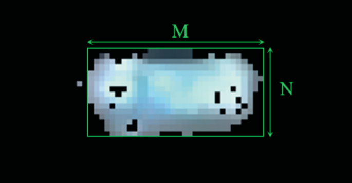
Definition of width and height of license plate

For the ith connected domain, M = width of the external rectangle, N = height of the external rectangle, length width ratio R = M/N.
That is to erase the ith connected domain.
-
Remove the connected region whose area is too small for the external rectangle.
A highly efficient algorithm, which recognizes the license plate connection domain, pixel points should be dense enough, rather than full of holes. The proportion of the area of the connected domain to the outside rectangle is not too low. In this chapter, the area ratio is within [0.53, 1], and 0.53 is the minimum value that can be tolerated.
For the ith connected domain, M = width of the external rectangle, N = height of the external rectangle, and the area of the connected domain is S, RR = S/(M × N).
That is to erase the ith connected domain.
The label process of the filtered I_lp is the same as that of the tail lamp, and the center coordinates of the rectangle outside the connected region of I_lp are calculated.
6 Generation of Tail Lamp Confidence
In the tail light I_tl area divided by color, each connected region can match at most with another connected region. How can we judge which connected region i matches with the other connected regions with the highest probability of success? In this algorithm, the idea of I_tl confidence is introduced.
6.1 Obtaining Confidence
The number of connected domains in the filtered I_tl is numT, and a zero matrix of numt × numt is created.
Taking the data above the main diagonal, the number in row I, column J (J > I) indicates the confidence level of the relationship between the ith connected domain and the jth connected domain. Then set three conditions:
-
Symmetry
The abscissa of the center of the circumscribed rectangle of the ith I_lp is Lx(i), the abscissa of the center of the circumscribed rectangle of the ith I_tl is Tx (t), and the set of the abscissa of all the circumscribed rectangles of the ith I_tl is Tx. If the two taillights are matched successfully, there must be at least one license plate I_lp in the middle. The distance between them and Lx(i) of I_lp is less than a certain empirical value Δ (the empirical value is calibrated by the experiment) and the direction is opposite.
If the conditions of this layer are met in TX, the confidence level will be increased by one level. It should be noted that there may be more than one I_lp connected domain in the middle of a pair of taillights. For example, the I_lp satisfies the condition, and the I + 1th I_lp may also satisfy the condition. Therefore, if the frequency is greater than 1, frequency is 1, algorithm is needed to limit it.
-
Height difference
The horizontal height of the two taillights of the same car must not differ too much.
If the condition of this layer is satisfied, the confidence level will be increased one level.
-
Horizontal distance
The horizontal distance between the two taillights of the same vehicle must not be too much different. Based on the transverse coordinate Ty(I) of the outer rectangular center of the ith I_tl, find all the satisfied conditions in Ty:
If the condition of this layer is satisfied, the confidence level will be increased one level.
Finally, the tail lamp relationship pair with full confidence level is qualified to be combined with the license plate and successfully matched. The algorithm will find the connected region I_lp in the middle of the tail lamp pair, and frame three as the final recognition results.
6.2 Removal of Misidentification
However, there are still many mismatches in this confidence system, which can be divided into the following categories.
-
One for many
One tail lamp can only be matched with another under normal conditions, and it is impossible to match multiple tail lamps. In this algorithm, the basic reason for this situation is that there are multiple relationship pairs with full scores in the same row of the frequency matrix. So we need to judge more conditions to further limit the confidence.
As shown in Fig. 20 on the right, if there is one car with many cars, assume that the jth and j + 1th columns in the ith row are full marks at the same time, then it is necessary to determine which relationship pair is invalid. According to the first condition of confidence, if the full score can be obtained, then there must be I_lp in the middle of the taillight pair. Because the interference of the two correct tail lamp pairs is extremely low, the two tail lamps that are matched together should be the two closest to the I_lp.

One to many mismatches
According to this principle, other distant relation pairs can be eliminated, and TX (I), TX (J), TX (j + 1) can be taken as the difference and order with the horizontal coordinate LX of I OULP center respectively:
DR is the matrix after sorting from small to large, index is the sequence number before corresponding sorting, the first two corresponding frequencies are reserved, and other frequencies are eliminated, so that one to many mismatches can be eliminated.
-
Suspected light source interference
In the external environment, there are often interference light sources that are similar to the tail lamp in color and shape, such as billboards. They are separated from the tail lamp by the partial red field together with the tail lamp, and there may also be I_lp satisfying the conditions in the middle, so there is a possibility of mismatch. Mismatch of interference light source1.25 is shown in Fig. 21. Different from the tail lamp pair, the area of the two connected areas of the interference light source is often smaller and far away, so the principle that the larger the distance between the two tail lamps is, the larger the tail lamp area should be can be used to eliminate the mismatched lamp pair.

Mismatch of interference light source1.25
Definition of center distance and connected area is shown in Fig. 22. The connected area of the two taillights is tstats(1).Area and tstats(2).Area, and the center distance is set as X.Take:

Definition of center distance and connected area
In the tail lamp image segmented by this algorithm, for different x statistic Y values as far as possible, it should be noted that the smaller the Actual-area is, the less obvious the distance between vehicles in different lanes with the camera is (When x is getting bigger). The smaller the Actual-area is, the less obvious it is. On the contrary, the larger the X is, the more obvious the Actual-area is, so the trend line should be a nonlinear polynomial. In this paper, about 20 groups of X–Y data under different conditions are counted, and the number of statistics within [100200] is more, because the probability of error in this part is higher.
As shown in Fig. 23, Y represents the predicted-area, and the judgment relationship is:

Relationship between predicted-area and X
The largest connected area of two suspected taillight pairs is smaller than predicted area, so it is a non ideal relationship pair.
-
Resolve adhesion
When the red area in the image is too close, the algorithm is likely to identify them as the same tail lamp suspected area, and through layer by layer filtering, all conditions are met, and finally the matching is successful, as shown in Fig. 24. The solution is simple. For example, if the ith and jth match successfully and there is adhesion, it is only necessary to replace the length and width of the rectangle outside the larger connected domain with the length and width of another connected domain.

Adhesion
7 Final Experimental Results
With the check of the algorithm of eliminating false recognition, there are very times of missing or false detection.
In this paper, VC++ is used for experiment. Experimental results of the algorithm is shown in Fig. 25. The experiment results show that the recognition effect is good. The algorithm can accurately identify and frame the area including tail lamp and license plate. The detection and recognition rate of the algorithm on urban main roads and highways are shown in Table 5.

Experimental results of the algorithm
There are many non taillight interference light sources on urban main roads. There are 43 frames of 582 frames of video with false detection (including false detection and missing detection), which shows that the algorithm can effectively eliminate the influence of interference light source, and the situation of false detection is mostly that the taillight area is interfered by the front headlights, and the red area is covered by strong light, so it cannot be detected. Interference by headlights is shown in Fig. 26.

Interference by headlights
To summarize, in the case of less vehicles and less environmental interference, the recognition effect of the algorithm is very considerable.
References
Sun Z, Bebis G, Miller R (2004) On-road vehicle detection using optical sensors: a review. In: The international IEEE conference on intelligent transportation systems, 2004 proceedings. IEEE, Washington, DC, pp 585–590
Yu LY, Guo YL (2019) Method of preceding vehicle detection and tracking at night based on taillights. J Tianjin Polytech Univ 38(1):61–68
Liu ZY, Ye Q, Li F et al (2010) Taillight detection algorithm based on four thresholds of brightness and color. Comput Eng 36(21):202–203, 206 (in Chinese)
Tian XX, Wang JS (2016) Application of finite state machine in night time vehicle detection. J Shijiazhuang Tiedao Univ (Nat Sci) 29(4):95–99
Lin YC, Lin CC, Chen LT, Chen CK (2011) Adaptive IPM-based lane filtering for night forward vehicle detection. In: IEEE conference on industrial electronics and applications. ICIEA, Beijing
Xiao ZT, Wang Y, Geng L, Zhang F (2013) Preceding vehicle detecting method for night based on geometry and position features of blobs. J Hebei Univ Technol 42(5):13–18 (in Chinese)
Xu CC (2019) Denoising algorithm based on image histogram. Comput Internet 45(16):34–35
O’Malley R, Jones E, Glavin M (2010) Rear-lamp vehicle detection and tracking in low-exposure color video for night conditions. IEEE
Bao QL (2010) Colorful image segmentation based on HSV. Softw Guide 09(07):171–172
Qi QH, Chen QX (2012) Vehicle detection based on two-way multilane at night. Commun Technol 45(10):58–60
Tian Y (2009) Digital image processing and analysis. Huazhong University of Science and Technology Press, Wuhan
Author information
Authors and Affiliations
Corresponding author
Editor information
Editors and Affiliations
Rights and permissions
Copyright information
© 2022 The Author(s), under exclusive license to Springer Nature Singapore Pte Ltd.
About this paper

Cite this paper
Ma, G., Cai, M., Chen, G., Li, Z. (2022). Vehicle Detection at Night Based on the Feature of Taillight and License Plate. In: Wang, W., Chen, Y., He, Z., Jiang, X. (eds) Green Connected Automated Transportation and Safety. Lecture Notes in Electrical Engineering, vol 775. Springer, Singapore. https://doi.org/10.1007/978-981-16-5429-9_55
Download citation
DOI: https://doi.org/10.1007/978-981-16-5429-9_55
Published:
Publisher Name: Springer, Singapore
Print ISBN: 978-981-16-5428-2
Online ISBN: 978-981-16-5429-9
eBook Packages: EngineeringEngineering (R0)