Incentive Mechanisms for Federated Learning

Abstract

In this chapter, we discuss various components of federated learning that must be given some incentive in terms of monetary cost or other benefits. We design incentive mechanism design for federated learning using game theory and auction theory. Finally, we present extensive numerical results to show the validity of our proposed incentive mechanisms.

1 Introduction

Federated learning can be trained mainly in two different ways, such as (a) centralized server aggregation-based training, and (b) blockchain-based training, as shown in Figs. 4.1 and 4.2. Federated learning using centralized server aggregation involves continuous, iterative interaction between the end-devices and aggregation server. End-devices use their resources (i.e., computation resource and energy) to train their local learning models. The locally trained model updates will be sent via a wireless channel to the aggregation server for global aggregation. Similar to end-devices, the aggregation server will use its resources (i.e., computation resource and energy) to perform aggregation. To enable successful interaction among end-devices and aggregation servers for federated learning requires an attractive incentive mechanism. End-devices must be provided with benefits in response to their participation in the federated learning process. On the other hand, blockchain-based federated learning involves the computation of local models at the end-devices. The end-devices send their local learning models to their corresponding miners. The miners perform sharing and cross-verification of learning models to avoid injection of wrong models. Then, all the miners start computing their consensus algorithms (e.g., Proof-of-Work). The winning miner that solves the consensus algorithm first, broadcasts its block to all the miners in the network for updating their blocks. In blockchain-based federated learning, there is a need to provide an attractive incentive to both end-devices and miners for their jobs. Therefore, the incentive mechanism for blockchain-based federated learning will be different than the one for federated learning based on a centralized aggregation server.

Fig. 4.1

Overview of rewards in centralized aggregation-based federated learning

Fig. 4.2

Overview of rewards in blockchain-based federated learning

Generally, we can categorize incentives into two main types: monetary and non-monetary [100]. Monetary incentives are based on providing end-devices with payments as per their participation, whereas non-monetary incentives generally involve providing end-devices with benefits other than payments. Non-monetary incentives in the case of federated learning can be the well-trained global federated learning model for a large number of end-devices. Unless stated otherwise, the keyword incentive in this chapter refers to monetary incentive. Next, we present incentive mechanisms based on game theory and auction theory for federated learning over wireless networks.

2 Game Theory-Enabled Incentive Mechanism

Game theory has proven to be one of the successful tools in enabling/optimizing various functions/design aspects in wireless networks, such as wireless resource allocation, computational offloading in edge computing, URLLC/eMBB coexistence, and incentive mechanism design, among others [101,102,103,104,105]. Generally, games can be divided into (a) cooperative and (b) non-cooperative games. Cooperative games are based on achieving the equilibrium state for optimizing the overall benefit via joint decision-making by the various players. On the other hand, the players in non-cooperative games choose their strategies selfishly without coordination with other players (Fig. 4.3). A summary of cooperative and non-cooperative games used for incentive mechanism design in wireless networks is given in Table 4.1.

Fig. 4.3

Classification of game theoretic incentive mechanisms

Table 4.1 Overview of game theoretic incentive mechanisms [106]

In federated learning, local computations at the devices and their communication with the centralized coordinating server are interleaved in a complex manner to build a global learning model. Therefore, a communication-efficient federated learning framework [18, 58] requires solving several challenges. Furthermore, because of limited data per device to train a high-quality learning model, the difficulty is to incentivize a large number of mobile users to ensure cooperation. This important aspect in federated learning has been overlooked so far, where the question is how can we motivate a number of participating clients, collectively providing a large number of data samples to enable federated learning without sharing their private data? Note that both participating clients and the server can benefit from training a global model. However, to fully reap the benefits of high-quality updates, the multi-access edge computing (MEC) server has to incentivize clients for participation. In particular, under heterogeneous scenarios, such as an adaptive and cognitive-communication network, the client’s participation in federated learning can spur collaboration and provide benefits for operators to accelerate and deliver network-wide services [111]. Similarly, clients, in general, are not concerned with the reliability and scalability issues of federated learning [112]. Therefore, to incentivize users to participate in the collaborative training, we require a marketplace. For this purpose, we present a value-based compensation mechanism to the participating clients, such as a bounty (e.g., data discount package), as per their level of participation in the crowdsourcing framework. This is reflected in terms of local accuracy level, i.e., quality of solution to the local subproblem, in which the framework will protect the model from imperfect updates by restricting the clients trying to compromise the model (for instance, with skewed data because of its i.i.d nature or data poisoning) [113]. Moreover, we cast the global loss minimization problem as a primal-dual optimization problem, instead of adopting a traditional gradient descent learning algorithm in the federated learning setting (e.g., FedAvg [18]). This enables (a) proper assessment of the quality of the local solution to improve personalization and fairness amongst the participating clients while training a global model, (b) effective decoupling of the local solvers, thereby balancing communication and computation in the distributed setting.

The goal of this section is two-fold: First, we formalize an incentive mechanism to develop a participatory framework for mobile clients to perform federated learning for improving the global model. Second, we address the challenge of maintaining communication efficiency while exchanging the model parameters with a number of participating clients during aggregation. Specifically, communication efficiency in this scenario accounts for communications per iteration with an arbitrary algorithm to maintain an acceptable accuracy level for the global model. In this work, we design and analyze a novel crowdsourcing framework to realize the federated learning vision. Specifically, our contributions are summarized as follows:

• A crowdsourcing framework to enable communication -efficient federated learning. We design a crowdsourcing framework, in which federated learning participating clients iteratively solve the local learning subproblems for an accuracy level subject to an offered incentive. We then establish a communication-efficient cost model for the participating clients. We then formulate an incentive mechanism to induce the necessary interaction between the MEC server and the participating clients for the federated learning in Sect. 4.2.2.

• Solution approach using Stackelberg game. With the offered incentive, the participating clients independently choose their strategies to solve the local subproblem for a certain accuracy level in order to minimize their participation costs. Correspondingly, the MEC server builds a high-quality centralized model characterized by its utility function, with the data distributed over the participating clients by offering the reward. We exploit these tightly coupled motives of the participating clients and the MEC server as a two-stage Stackelberg game. The equivalent optimization problem is characterized as mixed-Boolean programming which requires an exponential complexity effort for finding the solution. We analyze the game’s equilibria and propose a linear complexity algorithm to obtain the optimal solution.

• Participant’s response analysis and case study. We next analyze the response behavior of the participating clients via the solutions of the Stackelberg game and establish the efficacy of our proposed framework via case studies. We show that the linear-complexity solution approach attains the same performance as the mixed-Boolean programming problem. Furthermore, we show that our mechanism design can achieve the optimal solution while outperforming a heuristic approach for attaining the maximal utility with up to 22% of gain in the offered reward.

• Admission control strategy. Finally, we show that it is significant to have certain participating clients to guarantee the communication efficiency for an accuracy level in federated learning. We formulate a probabilistic model for threshold accuracy estimation and find the corresponding number of participants required to build a high-quality learning model. We analyze the impact of the number of participants in federated learning while determining the threshold accuracy level with closed-form solutions. Finally, with numerical results, we demonstrate the structure of the admission control model for different configurations.

2.1 System Model

Figure 4.4 illustrates our proposed system model for the crowdsourcing framework to enable federated learning. The model consists of a number of mobile clients associated with a base station having a central coordinating server (MEC server), acting as a central entity. The server facilitates the computation of the parameters aggregation, and feedback the global model updates in each global iteration. We consider a set of participating clients $\mathcal {K} = \{1,2,\ldots ,K \}$ in the crowdsourcing framework. The crowdsourcer (platform) can interact with mobile clients via an application interface and aims at leveraging federated learning to build a global ML model. As an example, consider a case where the crowdsourcer (referred to as MEC server hereafter, to avoid any confusion) wants to build a ML model. Instead of just relying on available local data to train the global model at the MEC server, the global model is constructed utilizing the local training data available across several distributed mobile clients. Here, the global model parameter is first shared by the MEC server to train the local models in each participating client. The local model’s parameters minimizing local loss functions are then sent back as feedback and are aggregated to update the global model parameter. The process continues iteratively, until convergence.

Fig. 4.4

Crowdsourcing framework for decentralized machine learning

2.1.1 Federated Learning Background

For federated learning, we consider unevenly partitioned training data over a large number of participating clients to train the local models under any arbitrary learning algorithm. Each client k stores its local dataset $\mathcal {D}_k$ of size D _k respectively. Then, we define the training data size $D = \sum _{k=1}^{K}D_{k}$. In a typical supervised learning setting, $\mathcal {D}_k$ defines the collection of data samples given as a set of input-output pairs $\{x_i, y_i\}_{i=1}^{D_k}$, where $x_i \in \mathbb {R}^d$ is an input sample vector with d features, and $y_i \in \mathbb {R}$ is the labeled output value for the sample x _i. The learning problem, for an input sample vector x _i (e.g., the pixels of an image) is to find the model parameter vector $w\in \mathbb {R}^d$ that characterizes the output y _i (e.g., the labeled output of the image, such as the corresponding product names in a store) with the loss function f _i(w). Some examples of loss functions include $f_i(w) = \frac {1}{2}(x_i^Tw - y_i)^2, y_i \in \mathbb {R}$ for a linear regression problem and $f_i(w) = \max \{0, 1 -y_ix_i^Tw\},y_i \in \{-1,1\}$ for support vector machines. The term $x_i^Tw$ is often called a linear mapping function. Therefore, the loss function based on the local data of client k, termed local subproblem is formulated as

$$\displaystyle \begin{aligned} J_{k}(w) = \frac{1}{D_k} \sum \nolimits_{i = 1}^{D_k}f_i(w) + \lambda g(w), {} \end{aligned} $$

(4.1)

where $w\in \mathbb {R}^d$ is the local model parameter, and g(⋅) is a regularizer function, commonly expressed as $g(\cdot ) = \frac {1}{2}\left \lVert \cdot \right \rVert ^2$; ∀λ ∈ [0, 1]. This characterizes the local model in the federated learning setting.

Algorithm 4 Federated learning framework

Global Problem

At the MEC server, the global problem can be represented as the finite-sum objective of the form

(4.2)

Problems of such structure as in (4.2) where we aim to minimize an average of K local objectives are well-known as distributed consensus problems [114].

Solution Framework under Federated Learning

We recast the regularized global problem in (4.2) as

(4.3)

and decompose it as a dual optimization problem¹ in a distributed scenario [115] amongst K participating clients. For this, at first, we define $X \in \mathbb {R}^{d \times D_k}$ as a matrix with columns having data points for $i \in \mathcal {D}_k, \forall k$. Then, the corresponding dual optimization problem of (4.3) for a convex loss function f is

(4.4)

where $\alpha \in \mathbb {R}^{D}$ is the dual variable mapping to the primal candidate vector, $f_i^*$ and g ^∗ are the convex conjugates of f _i and g respectively [116]; $\phi (\alpha ) = \frac {1}{\lambda D} X \alpha$. With the optimal value of dual variable α ^∗ in (4.4), we have w(α ^∗) = ∇g ^∗(ϕ(α ^∗)) as the optimal solution of (4.3) [115]. For the ease of representation, we will use $\phi \in \mathbb {R}^d$ for ϕ(α) hereafter. We consider that g is a strongly convex function, i.e., g ^∗(⋅) is continuous differentiable. Then, the solution is obtained following an iterative approach to attain a global accuracy 0 ≤ 𝜖 ≤ 1 (i.e., $\mathbb {E}\left [ \boldsymbol {\mathcal {G}}(\alpha ) - \boldsymbol {\mathcal {G}}(\alpha ^*)\right ] < \epsilon$).

Under the distributed setting, we further define data partitioning notations for clients $k \in \mathcal {K}$ to represent the working principle of the framework. Let us define a weight vector $\varrho _{[k]} \in \mathbb {R}^D$ at the local subproblem k with its elements zero for the unavailable data points. Following the assumption of having f _i as (1∕γ)-smooth and 1-strongly convex of g to ensure convergence, its consequences is the approximate solution to the local problem k defined by the dual variables α _[k], ϱ _[k], characterized as

(4.5)

where $\boldsymbol {\mathcal {G}}_k (\varrho _{[k]}; \phi , \alpha _{[k]}) = -\frac {1}{K} - \langle \nabla (\lambda g^*(\phi (\alpha ))), \varrho _{[k]} \rangle - \frac {\lambda }{2} \Vert \frac {1}{\lambda D}X_{[k]}\varrho _{[k]} \Vert ^2$ is defined with a matrix X _[k] columns having data points for $i \in \mathcal {D}_k$, and zero padded otherwise. Each participating client $k \in \mathcal {K}$ iterates over its computational resources using any arbitrary solver to solve its local problem (4.5) with a local relative θ _k accuracy that characterizes the quality of the local solution, and produces a random output ϱ _[k] satisfying

$$\displaystyle \begin{aligned} \mathbb{E}\left[ \boldsymbol{\mathcal{G}}_k(\varrho^*_{[k]}) - \boldsymbol{\mathcal{G}}_k(\varrho_{[k]}) \right] \le \theta_k \left[ \boldsymbol{\mathcal{G}}_k(\varrho^*_{[k]}) - \boldsymbol{\mathcal{G}}_k(0) \right]. \end{aligned} $$

(4.6)

Note that, with local (relative) accuracy θ _k ∈ [0, 1], the value of θ _k = 1 suggests that no improvement was made by the local solvers during successive local iterations. Then, the local dual variable is updated as follows:

$$\displaystyle \begin{aligned} \alpha^{t+1}_{[k]} := \alpha^t_{[k]} + \varrho^t_{[k]},\forall k \in \mathcal{K}. {} \end{aligned} $$

(4.7)

Correspondingly, each participating client will broadcast the local parameter defined as $\varDelta \phi ^t_{[k]}:= \frac {1}{\lambda D} X_{[k]}\varrho ^t_{[k]}$, during each round of communication to the MEC server. The MEC server aggregates the local parameter (averaging) with the following rule:

$$\displaystyle \begin{aligned} \phi^{t+1} := \phi^t + \frac{1}{K}\sum \nolimits_{k = 1}^{K} \varDelta \phi^t_{[k]}, {} \end{aligned} $$

(4.8)

and distributes the global change in ϕ to the participating clients, which is used to solve (4.5) in the next round of local iterations. This way we observe the decoupling of global model parameter from the need of local clients’ data² for training a global model.

Algorithm 4 briefly summarizes the federated learning framework as an iterative process to solve the global problem characterized in (4.3) for a global accuracy level. The iterative process (S2)–(S8) of Algorithm 4 terminates when the global accuracy 𝜖 is reached. A participating client k strategically³ iterates over its local training data $\mathcal {D}_k$ to solve the local subproblem (4.5) up to an accuracy θ _k. In each communication round with the MEC server, the participating clients synchronously pass on their parameters Δϕ _[k] using a shared wireless channel. The MEC server then aggregates the local model parameters ϕ as in (4.8), and broadcasts the global parameters required for the participating clients to solve their local subproblems for the next communication round. Within the framework, consider that each participating client uses any arbitrary optimization algorithm (such as Stochastic Gradient Descent (SGD), Stochastic Average Gradient (SAG), Stochastic Variance Reduced Gradient (SVRG)) to attain a relative θ accuracy per local subproblem. Then, for strongly convex objectives, the number of iterations is dependent on local relative θ accuracy of the local subproblem and the global model’s accuracy 𝜖 as [58]:

$$\displaystyle \begin{aligned} I^{\mathrm{g}}(\epsilon,\theta) &= \frac{\zeta \cdot\log (\frac{1}{\epsilon})}{1-\theta}, {} \end{aligned} $$

(4.9)

where the local relative accuracy measures the quality of the local solution as defined in the earlier paragraphs. Further, in this formulation, we have replaced the term $\mathcal {O}(\log (\frac {1}{\epsilon }))$ in the numerator with $\zeta \cdot \log (\frac {1}{\epsilon })$, for a constant ζ > 0. For fixed iterations I ^g at the MEC server to solve the global problem, we observe in (4.9) that a very high local accuracy (small θ) can significantly improve the global accuracy 𝜖. However, each client k has to spend excessive resources in terms of local iterations, $I_k^{\mathrm {l}}$ to attain a small θ _k accuracy as

$$\displaystyle \begin{aligned} I_k^{\mathrm{l}}(\theta_k) = \gamma_k\log \bigg(\frac{1}{\theta_k}\bigg), {} \end{aligned} $$

(4.10)

where γ _k > 0 is a parameter choice of client k that depends on the data size and condition number of the local subproblem [58]. Therefore, to address this trade-off, MEC server can setup an economic interaction environment (a crowdsourcing framework) to motivate the participating clients for improving the local relative θ _k accuracy. Correspondingly, with the increased reward, the participating clients are motivated to attain better local θ _k accuracy, which as observed in (4.9) can improve the global 𝜖 accuracy for a fixed number of iterations I ^g of the MEC server to solve the global problem. In this scenario, to capture the statistical and system-level heterogeneity, the corresponding performance bound in (9) for heterogeneous responses θ _k can be modified considering the worst-case response of the participating client as

$$\displaystyle \begin{aligned} I^{\mathrm{g}}(\epsilon,\theta_k) = \frac{\zeta \cdot \log(\frac{1}{\epsilon})}{1 - {\max}_k\ \theta_k}, \forall k \in \mathcal{K}. {} \end{aligned} $$

(4.11)

Figure 4.5 describes an interaction environment incorporating a crowdsourcing framework and federated learning setting. In the following section, we will further discuss in detail the proposed incentive mechanism and present the interaction between the MEC server and participating clients as a two-stage Stackelberg game.

Fig. 4.5

Interaction environment of federated learning setting under crowdsourcing framework

2.1.2 Cost Model

Training on local data for a defined accuracy level incurs a cost for the participating clients. We discuss its significance with two typical costs: the computing cost and the communication cost.

Computing Cost

This cost is related to the number of iterations performed by client k on its local data to train the local model for attaining a relative accuracy of θ _k in a single round of communication. With (4.10), we define the computing cost for client k when it performs computation on its local data $\mathcal {D}_k$.

Communication Cost

This cost is incurred when client k interacts with MEC server for parameter updates to maintain θ _k accuracy. During a round of communication with the MEC server, let e _k be the size (in bits) of local parameters $\varDelta \phi _{[k]}, k \in \mathcal {K}$ in a floating-point representation produced by the participating client k after processing a mini-batch [118]. While e _k is the same for all the participating clients under a specified learning setting of the global problem, each participating client k can invest resources to attain specific θ _k as defined in (4.10). Although the best choice would be to choose θ _k such that the local solution time is comparable with the time expense in a single communication round, larger θ _k will induce more rounds of interaction between clients until global convergence, as formalized in (4.9).

With the inverse relation of global iteration upon local relative accuracy in (4.9), we can characterize the total communication expenditure as

$$\displaystyle \begin{aligned} T(\theta_k) = \frac{T_k}{(1 - \theta_k)}, {} \end{aligned} $$

(4.12)

where T _k as the time required for the client k to communicate with MEC server in each round of model’s parameter exchanges. Here, we normalize ζ > 0 in (4.9) to 1 as the constant can be absorbed into T _k for each round of model’s parameter exchanges when we characterize the communication expenditure in (4.12). Using first-order Taylor’s approximation,⁴ we can approximate the total communication cost as T(θ _k) = T _k ⋅ (1 + θ _k). We assume that clients are allocated orthogonal sub-channels so that there is no interference between them.⁵ Therefore, the instantaneous data rate for client k can be expressed as

$$\displaystyle \begin{aligned} R_k = B \log_2 \left(1 + \frac{p_k |G_k|{}^2}{\mathcal{N}_k}\right), \forall k \in \mathcal{K}, {} \end{aligned} $$

(4.13)

where B is the total bandwidth allocated to the client k, p _k is the transmission power of the client k, |G _k|² is the channel gain between participating client k and the base station, and $\mathcal {N}_k$ is the Gaussian noise power at client k. Then for client k, using (4.13), we can characterize T _k for each round of communication with the MEC server to upload the required updates as

$$\displaystyle \begin{aligned} T_k = \frac{e_k}{B \log_2 \left(1 + \frac{p_k |G_k|{}^2}{\mathcal{N}_k}\right)}, \forall k \in \mathcal{K}. {} \end{aligned} $$

(4.14)

(4.14) provides the dependency of T _k on wireless conditions and network connectivity.

Assimilating the rationale behind our earlier discussions, for a participating client with evaluated T _k, the increase in value of θ _k (poor local accuracy) will contribute to a larger communication expenditure. This is because the participating client has to interact more frequently with the MEC server (increased number of global iterations) to update its local model parameter for attaining relative θ _k accuracy. Further, the authors in [119] have provided the convergence analysis to justify this relationship and the communication cost model, though with a different technique.

Therefore, the participating client k’s cost for the relative accuracy level θ _k on the local subproblem is

$$\displaystyle \begin{aligned} C_k(\theta_k)& = (1+\theta_k ) \cdot \left(\nu_k \cdot T_k + (1 - \nu_k)\cdot \gamma_k \log\bigg(\frac{1}{\theta_k}\bigg)\right), \\ \end{aligned} $$

(4.15)

where 0 ≤ ν _k ≤1 is the normalized monetary weight for communication and computing costs (i.e., $/ rounds of iteration). A smaller value of relative accuracy θ _k indicates a high local accuracy. Thus, there exists a trade-off between the communication and the computing cost (4.15). A participating client can adjust its preference on each of these costs with the weight metric ν _k. The higher value of ν _k emphasizes the larger rounds of interaction with the MEC server to adjust its local model parameters for the relative θ _k accuracy. On the other hand, the higher value of (1 − ν _k) reflects the increased number of iterations at the local subproblem to achieve the relative θ _k accuracy. This will also significantly reduce the overall contribution of communication expenditure in the total cost formulation for the client. Note that the client cost over iterations could not be the same. However, to make the problem more tractable, according to (9) we consider minimizing the upper-bound of the cost instead of the actual cost, similar to approach in [111].

2.2 Stackelberg Game-Based Solution

In this section, firstly, we present our motivation to realize the concept of federated learning by employing a crowdsourcing framework. We next advocate an incentive mechanism required to realize this setting of decentralized learning model with our proposed solution approach.

2.2.1 Incentive Mechanism: A Two-Stage Stackelberg Game Approach

The MEC server will allocate rewards to the participating clients to achieve optimal local accuracy in consideration for improving the communication efficiency of the system. That means the MEC server will plan to incentivize clients for maximizing its own benefit, i.e., an improved global model. Consequently, upon receiving the announced reward, any rational client will individually maximize their own profit. Such an interaction scenario can be realized with a Stackelberg game approach.

Specifically, we formulate our problem as a two-stage Stackelberg game between the MEC server (leader) and participating clients (followers). Under the crowdsourcing framework, the MEC server designs an incentive mechanism for participating clients to attain a local consensus accuracy level⁶ on the local models while improving the performance of a centralized model. The MEC server cannot directly control the participating clients to maintain a local consensus accuracy level and requires an effective incentive plan to enroll clients for this setting.

Clients (Stage II)

The MEC server has an advantage, being a leader with the first-move advantage influencing the followers for participation with a local consensus accuracy. It will at first announce a uniform reward rate⁷ (e.g., a fair data package discount as $/accuracy level) r > 0 for the participating clients. Given r, at Stage II, a rational client k will try to improve the local model’s accuracy for maximizing its net utility by training over the local data with global parameters. The proposed utility framework incorporates the cost involved while a client tries to maximize its own individual utility.

Client Utility Model

We use a valuation function v _k(θ _k) to denote the model’s effectiveness that explains the valuation of the client k when relative θ _k accuracy is attained for the local subproblem.

Assumption 1

The valuation function v _k(θ _k) is a linear, decreasing function with θ _k > 0, i.e., v _k(θ _k) = (1 − θ _k). Intuitively, for a smaller relative accuracy at the local subproblem, there will be an increase in the reward for the participating clients.

Given r > 0, each participating client k’s strategy is to maximize its own utility as follows:

(4.16)

given cost C _k(θ _k) as (4.15). The feasible solution is always restricted to the value less than 1 (i.e., without loss of generality, for θ _k > 1, it violates the participation assumption for the crowdsourcing framework). Therefore, problem (4.16) can be represented as

(4.17)

Also, we have $C^{\prime \prime }_k(\theta _k) > 0$, which means C _k(θ _k) is a strictly convex function. Thus, there exists a unique solution $\theta _k^*(r), \forall k.$

MEC Server (Stage I)

Knowing the response (strategy) of the participating clients, the MEC can evaluate an optimal reward rate r ^∗ to maximize its utility. The utility U(⋅) of the MEC server can be defined in relation to the satisfaction measure achieved with the local consensus accuracy level.

MEC Server Utility Model

We define x(𝜖) as the number of iterations required for an arbitrary algorithm to converge to some 𝜖 accuracy. We similarly define I ^g(𝜖, θ) as global iterations of the framework to reach a relative θ accuracy on the local subproblems.

From this perspective, we require an appropriate utility function U(⋅) as the satisfaction measure of the framework with respect to the number of iterations for achieving 𝜖 accuracy. In this regard, use the definition of the number of iterations for 𝜖 accuracy as

$$\displaystyle \begin{aligned}x(\epsilon) = \zeta \cdot\log\bigg(\frac{1}{\epsilon}\bigg).\end{aligned}$$

Due to large values of iterations, we approximate x(𝜖) as a continuous value, and with the aforementioned relation, we choose U(⋅) as a strictly concave function of x(𝜖) for 𝜖 ∈ [0, 1], i.e., with the increase in x(𝜖), U(⋅) also increases. Thus, we propose U(x(𝜖)) as the normalized utility function bounded within [0, 1] as

$$\displaystyle \begin{aligned} U(x(\epsilon)) = 1 - 10^{-(ax(\epsilon)+b)},\ \ \ a \ge 0,b \le 0, {} \end{aligned} $$

(4.18)

which is strictly increasing with x(𝜖), and represents the satisfaction of MEC increase with respect to accuracy 𝜖.

As for the global model, there exists an acceptable value of threshold accuracy measure correspondingly reflected by $x_{\min }(\epsilon )$. This suggests the possibility of near-zero utility for the MEC server for failing to attain such value.

Figure 4.6 depicts our proposed utility function, a concave function of x(𝜖) with parameters a and b that reflect the required behavior of the utility function defined in (4.18). In Fig. 4.6, we can observe that a larger value of a means smaller iterations requirement and larger values of b introduces flat curves suggesting more flexibility in accuracy. So we can analyze the impact of parameters a and b in (4.18), and set them to model the utility function for the MEC server as per the design requirements of the learning framework. Furthermore, in our setting, I ^g(𝜖, θ) can be written as

$$\displaystyle \begin{aligned} & I^{\mathrm{g}}(\epsilon,\theta) = \frac{x(\epsilon)}{1-\theta} \le \delta. {} \end{aligned} $$

(4.19)

Fig. 4.6

MEC utility U(⋅) as a function of 𝜖 with different parameter values of a, b

(4.19) explains the efficiency paradigm of the proposed framework in terms of time required for the convergence to some accuracy 𝜖. If τ ^l(θ) is the time per iteration to reach a relative θ accuracy at a local subproblem and T(θ) is the communication time required during a single iteration for any arbitrary algorithm, then we can analyze the result in (4.19) with the efficiency of the global model as

$$\displaystyle \begin{aligned} & I^{\mathrm{g}}(\epsilon, \theta) \cdot (T(\theta)+ \tau^{\mathrm{l}}(\theta)). {} \end{aligned} $$

(4.20)

Because the cost of communication is proportional to the speed and energy consumption in a distributed scenario [123], the bound defined in (4.19) explains the efficiency in terms of the MEC server’s resource restriction for attaining 𝜖 accuracy. In this regard, the corresponding analysis of (4.20) is presented in the upcoming sub-section with several case studies.

The utility of the MEC server can therefore be defined for the set of measured best responses θ ^∗ as

$$\displaystyle \begin{aligned}\mathcal{U}(x(\epsilon),r| \boldsymbol{\theta}^*) = \beta \left(1 - 10^{-(ax(\epsilon)+b)} \right) - r \sum_{k \in \mathcal{K}} (1 - \theta^*_k(r)),\end{aligned}$$

where β > 0 is the system parameter,⁸ and $r \sum _{k \in \mathcal {K}} (1 - \theta ^*_k(r))$ is the cost spent for incentivizing participating clients in the crowdsourcing framework for federated learning. So, for the measured θ ^∗ from the participating clients at the MEC server, the utility maximization problem can be formulated as follows:

(4.21)

$$\displaystyle \begin{aligned} \text{s.t.}\qquad & \frac{x(\epsilon)}{1-{\max}_k\ \theta^*_k(r)} \le \delta. {} \end{aligned} $$

(4.22)

In constraint (4.22), ${\max }_k\ \theta ^*_k(r)$ characterizes the worst-case response for the server-side utility maximization problem with the bound on permissible global iterations. Note that MEC adapts admission control strategy (discussed in Sect. 4.2.3) to improve the number of participants for maximizing its utility. In fact, MEC has to increase the reward rate to maintain the minimum number of participation (at least two) to realize the distributed optimization setting in federated learning. In addition to this, the framework may suffer from slower convergence due to less participation. Thus, MEC will avoid deliberately dropping the clients to achieve a faster consensus with (4.22).

Furthermore, using the relationship defined in (4.19) between x(𝜖) and relative θ accuracy for the subproblem, we can analyze the impact of responses θ on MEC server’s utility in a federated learning setting with the constraint (4.11). To be more specific about this relation, we can observe that with the increased value of (1 − θ), i.e., lower relative accuracy (high local accuracy), the MEC server can attain better utility due to the corresponding increment in the value of x(𝜖). Note that in the client cost problem, x(𝜖) is treated as a constant provided by the MEC problem, and can be ignored for solving (4.16).

Lemma 1

The optimal solution x ^∗(𝜖) for (4.21) can be derived as $\delta (1- {\max }_k \ \theta ^*_k(r))$.

Proof

See Appendix.

Therefore, for the given θ ^∗(r), we can formalize (4.21) as

(4.23)

Stackelberg Equilibrium

With a solution to MEC server’s utility maximization problem, r ^∗ we have the following definition.

Definition 1

For any values of r, and θ, (r ^∗, θ ^∗) is a Stackelberg equilibrium if it satisfies the following conditions:

$$\displaystyle \begin{aligned} &\mathcal{U}(r^*,\boldsymbol{\theta}^*) \ge \mathcal{U}(r,\boldsymbol{\theta}^*), {} \end{aligned} $$

(4.24)

$$\displaystyle \begin{aligned} & u_k(\theta_k^*,r^*) \ge u_k(\theta_k,r^*), \ \forall k. {} \end{aligned} $$

(4.25)

Next, we employ the backward-induction method to analyze the Stackelberg equilibria: the Stage-II problem is solved at first to obtain θ ^∗, which is then used for solving the Stage-I problem to obtain r ^∗.

2.2.2 Stackelberg Equilibrium: Algorithm and Solution Approach

Intuitively, from (4.19), we see that the server can evaluate the maximum value of x(𝜖) required for attaining accuracy 𝜖 for the centralized model while maintaining relative accuracy θ _th amongst the participating clients. Here, θ _th is a consensus on a maximum local accuracy level amongst participating clients, i.e., the local subproblems will maintain at least θ _th relative accuracy. So, with the measured responses θ from the participating clients, the server can design a proper incentive plan to improve the global model while maintaining the worst-case relative accuracy ${\max }_k \ \theta ^*_k$ as θ _th for the local model.

Since the threshold accuracy θ _th can be adjusted by the MEC server for each round of solution, each participating client will maintain a response towards the maximum local consensus accuracy θ _th. This formalizes the client’s selection criteria [see Remark 1.] which is sufficient enough for the MEC server to maintain the accuracy 𝜖. We also have the lower bound related with the value of $x_{\min }(\epsilon )$ for equivalent accuracy $\epsilon _{\max }$ while dealing with the client’s responses θ, i.e.,

$$\displaystyle \begin{aligned} \log\left( \frac{1}{\epsilon_{\max}}\right) \le \frac{x(\epsilon)}{(1-\theta_{\mathrm{th}})} \le \delta_{\max}. {} \end{aligned} $$

(4.26)

where $\delta _{\max }$ is the maximum permissible upper bound to the global iterations.

As explained before and with (4.26), the value of θ _th can be varied (lowered) by MEC server to improve the overall performance of the system. For a worst case scenario, where the offered reward r for the client k is insufficient to motivate it for participation with improved local relative accuracy, we might have ${\max }_k\ \theta ^*_k(r) = 1$, i.e., θ _th = 1, no participation.

Lemma 2

For a given reward rate r, and T _k which is determined based upon the channel conditions (4.14), we have the unique solution $\theta ^*_k(r)$ for the participating client satisfying following relation:

$$\displaystyle \begin{aligned} g_k(r) = \log(e^{1/\theta^*_k (r)}\theta^*_k (r)), \forall k \in \mathcal{K}, {} \end{aligned} $$

(4.27)

for g _k(r) ≥ 1, where,

$$\displaystyle \begin{aligned}g_k(r) = \left[ \frac{r + \nu_k T_k}{(1 - \nu_k)\gamma_k} -1 \right].\end{aligned} $$

Proof

Because $C_k^{\prime \prime }(\theta _k) > 0$ for θ _k > 0, (4.17) is a strictly convex function resulted as a linear plus convex structure. Therefore, by the first-order condition, (4.17) can be deduced as

$$\displaystyle \begin{aligned} \frac{\partial u_k(r,\theta_k)}{\partial \theta_k}& = 0 \\ & \Leftrightarrow \frac{1}{\theta_k} - \log\bigg(\frac{1}{\theta_k}\bigg) = \left[\frac{r + \nu_kT_k}{(1- \nu_k)\gamma_k} -1\right],\\ & \Leftrightarrow \log(e^{1/\theta_k}\theta_k) = g_k(r). {} \end{aligned} $$

(4.28)

We observe that Lemma 2 is a direct consequence of the solution structure derived in (4.28). Hence, we conclude the proof.

From Lemma 2, we have some observations with the definition of g _k(r) for the response of the participating clients. First, we can show that $\theta ^*_k$ is larger for the poor channel condition on a given reward rate. Second, in such scenario, with the increase in reward rate, say for g _k(r) > 2 the participating clients will iterate more during their computation phase resulting in lower $\theta ^*_k$. This will reduce the number of global iterations to attain an accuracy level for the global problem.

We can therefore characterize the participating client k’s best response under the proposed framework as

$$\displaystyle \begin{aligned} \theta_k^*(r) & = \min \left\lbrace \hat{\theta}_k (r) \mid_{g_k(r) = \log(e^{1/\hat{\theta}_k(r)}\hat{\theta}_k(r))}, \theta_{\mathrm{th}} \right\rbrace, \forall k. {} \end{aligned} $$

(4.29)

(4.29) represents the best response strategy for the participating client k under our proposed framework. Intuitively, exploring the logarithmic structure in (4.27), we observe that the increase in incentive r will motivate participating clients to increase their efforts for local iteration in one global iteration. This is reflected by a better response, i.e., a lower relative accuracy (high local accuracy) during each round of communication with the MEC server.

Figure 4.7 illustrates such strategic responses of the participating clients over an offered reward for a given configuration. In this scenario, to elaborate the best response strategy as characterized in (4.29), we have considered four participating clients with different preferences (e.g., Client 3 being the most reluctant participant). We observe that Client 3 seeks more incentive r to maintain a comparable accuracy level as Client 1. Further, we consider the tradeoff between communication cost and the computation cost as discussed with the relation in (4.15). These costs are complementary in relation by ν _k, and for each client k their preferences upon these costs are also different. For instance, the higher value of ν _k for client k emphasizes the increased number of communication with the MEC server to improve the local relative accuracy θ _k.

Fig. 4.7

An illustration showing participating clients response over the offered reward rate

In Figs. 4.8, 4.9, and 4.10, we briefly present the solution analysis to (4.27) with the impact of channel condition (we define it as communication adversity) on the local relative accuracy for a constant reward. For this, in Fig. 4.8 we consider a participating client with the fixed offered reward setting r from uniformly distributed values of 0.1–5. We use normalized T _k parameter for a client k to illustrate the response analysis scenario. In Figs. 4.9 and 4.10, T _k is uniformly distributed on [0.1, 1], and ν _k is set at 0.6. Intuitively, as in Fig. 4.8, the increase in communication time T _k for a fixed reward r will influence participating clients to iterate more locally for improving local accuracy than to rely upon the global model, which will minimize their total cost. Under this scenario, we observe the increase in communication cost with the increase in communication time T _k. Thus, the clients will iterate more locally. However, the trend is significantly affected by normalized weights ν _k, as observed in Figs. 4.9 and 4.10. For a larger value of T _k (poor channel condition) as in the case of Fig. 4.10, increasing the value of ν _k, i.e., clients with more preference on the communication cost in the total cost model results to higher local iterations for solving local subproblems, as reflected by the better local accuracy, unlike in Fig. 4.9. In both cases we observe the decrease in communication cost upon participation. However, in Fig. 4.10 the communication cost is higher because of an expensive data rate. Therefore, for a given r, client k can adjust its weight metrics accordingly to improve the response θ _k.

Fig. 4.8

Solution Analysis (4.27) (Left Y-axis: Relative accuracy, Right Y-axis: Communication cost): impact of communication adversity on local relative accuracy for a constant reward

Fig. 4.9

Solution Analysis (4.27) (Left Y-axis: Relative accuracy, Right Y-axis: Communication cost): normalized weight versus relative accuracy for a fair data rate (quality communication channel)

Fig. 4.10

Solution Analysis (4.27) (Left Y-axis: Relative accuracy, Right Y-axis: Communication cost): normalized weight versus relative accuracy for an expensive data rate

In Figs. 4.11, 4.12, and 4.13, we explore such behaviors of the participating clients through the heatmap plot. To explain better, we define three categories of participating clients based upon the value of normalized weights ν _k, ∀k, which are their individual preferences upon the computation cost and the communication cost for the convergence of the learning framework. (i) Reluctant clients with a lower ν _k consume more reward to improve local accuracy, even though the value of T _k is larger (expensive), as observed in Fig. 4.11. (ii) Sensitive clients are more susceptible towards the channel quality with larger ν _k, and iterates more locally within a round of communication to the MEC server for improving local accuracy, as observed in Fig. 4.13. (iii) Rational clients, as referred in Fig. 4.12 tend to balance these extreme preferences (say ν _k = 0.5 for client k), which in fact would be unrealistic to expect all the time due to heterogeneity in participating client’s resources.

Fig. 4.11

Case Study: impact of communication cost and offered reward rate r for normalized weight (preferences), reluctant clients i.e., ν _k = 0.1. X-axis shows the increase in incentive (r) value from left-to-right, and the y-axis defines the increase in value of communication expenditure (top-to-bottom)

Fig. 4.12

Case Study: impact of communication cost and offered reward rate r for normalized weight (preferences), rational clients, ν _k = 0.7. X-axis shows the increase in incentive (r) value from left-to-right, and the y-axis defines the increase in value of communication expenditure (top-to-bottom)

Fig. 4.13

Case Study: impact of communication cost and offered reward rate r for normalized weight (preferences), sensitive clients, ν _k = 0.7. X-axis shows the increase in incentive (r) value from left-to-right, and the y-axis defines the increase in value of communication expenditure (top-to-bottom)

To solve (4.23) efficiently, with (4.29) $\theta _k^*(r) =\min \left \lbrace \ \hat {\theta }_k (r) \mid _{g_k(r) = \log (e^{1/\hat {\theta }_k(r)}\hat {\theta }_k(r))},\right .$ we introduce a new variable z _k in relation with consensus on local relative accuracy θ _th,

$$\displaystyle \begin{aligned} z_k = \begin{cases} 1, & \text{if } \ r > \ \hat{ r }_k ; \\ 0, & \text{otherwise}, \end{cases} {} \end{aligned} $$

(4.30)

where

$$\displaystyle \begin{aligned}\hat{ r }_k = \left[ g_k^{-1}(\log(e^{1/\theta_{\mathrm{th}}}\theta_{\mathrm{th}})) \right]\end{aligned}$$

is the minimum incentive value required obtained from (4.29) to attain the local consensus accuracy θ _th at client k for the defined parameters ν _k and T _k.

This means, θ _k(r) < θ _th when z _k = 1, and θ _th ≤ θ _k(r) < 1 when z _k = 0. MEC server can use this setting to drop the participants with poor accuracy. As discussed before, for the worst case scenario we consider θ _th = 1.

Therefore, the utility maximization problem can be equivalently written as

(4.31)

$$\displaystyle \begin{aligned} \text{s.t.} & \qquad r \ge 0, {} \end{aligned} $$

(4.32)

$$\displaystyle \begin{aligned} & \qquad z_k \in \{0,1\}, \forall k. {} \end{aligned} $$

(4.33)

Algorithm 5 MEC server’s utility maximization

The problem (4.31) is a mixed-Boolean programming, which may require exponential-complexity effort (i.e., 2^K configuration of $\{z_k\}_{k \in \mathcal {K}}$) to solve by the exhaustive search. To solve this problem with linear complexity, we refer to the solution approach as in Algorithm 5.

The utility maximization problem at MEC server can be reformulated as a constraint optimization problem (4.34–4.35) assuming a fixed configuration of $\{z_k =1\}_{k \in \mathcal {K}}$ as

(4.34)

$$\displaystyle \begin{aligned} \text{s.t.}\qquad & r \sum_{k \in K} (1 - \theta^*_k(r)) \le B, {} \end{aligned} $$

(4.35)

where (4.35) is budget constraint for the problem. The second-order derivative of function $r(1 - \theta ^*_k(r))$ in (4.35) is $\frac {2\gamma _k(1- \nu _k)\nu _k T_k}{(r + \nu _k T_k)^3} > 0$, i.e., the problem (4.34) is a convex problem and can be solved similarly with Algorithm 5 (line 4–5).

Proposition 1

Algorithm 2 can solve the Stage-I equivalent problem (4.23) with linear complexity.

Proof

As the clients are sorted in the order of increasing $\hat {r}_k$ (line 1), for the sufficient condition $r > \hat {r}_k$ resulting z _k = 1, the MEC’s utility maximization problem reduces to a single-variable problem that can be solved using popular numerical methods.

Remark 1

Algorithm 2 can maintain consensus accuracy by formalizing the clients selection criteria. This is because from (4.30), z _k = 1 for θ _k(r) < θ _th, and z _k = 0 for θ _th ≤ θ _k(r) < 1. Thus, MEC server uses this setting to drop the participants with $\theta _k(r) > \theta _k^*(r) = \theta _{\mathrm {th}}$.

Theorem 1

The Stackelberg equilibria of the crowdsourcing framework are the set of pairs {r ^∗, θ ^∗}.

Proof

For any given θ, it is obvious that $\mathcal {U}(r^*, \boldsymbol {\theta }) \ge \mathcal {U}(r, \boldsymbol {\theta }), \forall r$ since r ^∗ is the solution to the Stage-I problem. Thus, we have $\mathcal {U}(r^*,\boldsymbol {\theta }^*) \ge \mathcal {U}(r, \boldsymbol {\theta }^*)$. In the similar way, for any given value of r and ∀k, we have $u_k(r,\theta _k^*) \ge u_k(r,\theta _k), \forall \theta _k$. Hence, $u_k(r^*,\theta _k^*) \ge u_k(r^*,\theta _k)$. Combining these facts, we conclude the proof being based upon the definitions of (4.24) and (4.25).

2.3 Simulations

In this section, we present numerical simulations to illustrate our results. We consider the learning setting for a strongly convex model such as logistic regression, as discussed in Sect. 4.2.1, to characterize and demonstrate the efficacy of the proposed framework. First, we will show the optimal solution of Algorithm 5 (Algorithm 5) and conduct a comparison of its performance with two baselines. The first one, named OPT, is the optimal solution of problem (4.23) with an exhaustive search for the optimal response θ ^∗. The second one is called Baseline that considers the worst response amongst the participating clients to attain local consensus θ _th accuracy with an offered price. This is an inefficient scheme but still enables us to attain feasible solutions. Finally, we analyze the system performance by varying different parameters and conduct a comparison of the incentive mechanism with the baseline and their corresponding utilities. In our analysis, the smaller values of local consensus are of specific interest as they reflect the effectiveness of federated learning.

• 1. Settings: For an illustrative scenario, we fix the number of participating clients to 4. We consider the system parameter β = 10, and the upper bound to the number of global iterations δ = 10, which characterizes the permissible rounds of communication to ensure global 𝜖 accuracy. The MEC’s utility U(x(𝜖)) = 1 − 10^{−(ax(𝜖)+b)} model is defined with parameters a = 0.3, and b = 0. For each client k, we consider normalized weight ν _k is uniformly distributed on [0.1,0.5], which can provide an insight on the system’s efficacy as presented in Figs. 4.11, 4.12, and 4.13. We characterize the interaction between the MEC server and the participating clients under homogeneous channel condition, and use the normalized value of T _k for all participating clients.

• 2. Reward rate: In Fig. 4.14 we increase the value of local consensus accuracy θ _th from 0.2 to 0.6. When the accuracy level is improved (from 0.4 to 0.2), we observe a significant increase in the reward rate. These results are consistent with the analysis in section “Stackelberg Equilibrium: Algorithm and Solution Approach”. The reason is that cost for attaining a higher local accuracy level requires more local iterations, and thus the participating clients exert more incentive to compensate for their costs.

  Fig. 4.14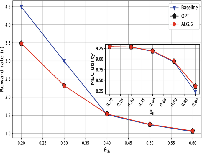

  

  Comparison of (a) Reward rate and (b) MEC utility under three schemes for different values of threshold θ _th accuracy

  We also show that the reward variation is prominent for lower values of θ _th, and observe that scheme Algorithm 2 and OPT achieve the same performance, while Baseline is not as efficient as others. Here, we can observe up to 22% gain in the offered reward against the Baseline by other two schemes. In Fig. 4.14b, we see the corresponding MEC utilities for the offered reward that complements the competence of the proposed Algorithm 2. We see, the trend of utility against the offered reward goes along with our analysis.

• 3. Parametric choice: In Figs. 4.15 and 4.16 we show the impact of parametric choice adopted by the participating client k to solve the local subproblem [124], which is characterized by γ _k. In Fig. 4.15, we see a lower offered reward for the improved local accuracy level for the participating clients adapting same parameters (algorithms) for solving the local subproblem, in contrast to Fig. 4.16 with the uniformly distributed γ _k on [1,5] to achieve the competitive utility.

  Fig. 4.15

  

  For $|\mathcal {K}| = 4, a= 0.3, b= 0$, γ _k = 1, ∀k

  Fig. 4.16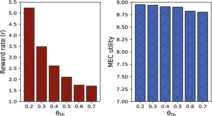

  

  For $|\mathcal {K}| = 4, a= 0.3, b= 0$, and γ _k ∼ U[1, 5]

• 4. Comparisons: In Tables 4.2 and 4.3, we see the effect of randomized parameter γ _k for different configuration of MEC utility model U(⋅) defined by (a, b). For the smaller values of θ _th, which captures the competence of the proposed mechanism, we observe that the choice of (a, b) provides a consistent offered reward for improved utility from (0.35, −1) to (0.65, −1), which follows our analysis in section “Incentive Mechanism: A Two-Stage Stackelberg Game Approach”. For larger values of θ _th, we also see the similar trend in MEC utility. For a randomized setting, we observe up to 71% gain in offered reward against the Baseline, which validates our proposal’s efficacy aiding federated learning.

  Table 4.2 Offered reward rate comparison with randomized γ effect for different (a, b) setting

  Table 4.3 Utility comparison with randomized γ effect for different (a, b) setting

Our earlier discussion in Sect. 4.2.2 and simulation results explain the significance of choosing a local θ _th accuracy to build a global model that maximizes the utility of the MEC server. In this regard, at first, the MEC server evokes admission control to determine θ _th and the final model is learned later. This means, with the number of expected clients, it is crucial to appropriately select a proper prior value of θ _th that corresponds to the participating client’s selection criteria for training a specific learning model. Note that, in each communication round of synchronous aggregation at the MEC server, the quality of local solution benefits to evaluate the performance at the local subproblem. In this section, we will discuss about the probabilistic model employed by the MEC server to determine the value of the consensus θ _th accuracy.

We consider the local θ accuracy for the participating clients is an i.i.d and uniformly distributed random variable over the range $[ \theta _{\min }, \theta _{\max } ]$, then the PDF of the responses can be defined as $f_{\boldsymbol {\theta }}(\theta ) = \frac {1}{\theta _{\max } - \theta _{\min }}$. Let us consider a sequence of discrete time slots t ∈{1, 2, …}, where the MEC server updates its configuration for improving the accuracy of the system. Following our earlier definitions, at time slot t, the number of participating clients in the crowdsourcing framework for federated learning is $|\mathcal {K}(t)|$, or simply K. We restrict the clients with the accuracy measure $\boldsymbol {\theta }(t) \ge \theta _{\max }$. For K number of participation requests, the total number of accepted responses N(t) is defined as N(t) = K ⋅ F _θ(t)(θ) = K ⋅ P[θ(t) ≤ θ]. We have $N(t) = K \cdot \left [\frac {\theta (t) - \theta _{\min }}{\theta _{\max } - \theta _{\min }} \right ]$. At each time t, the MEC server chooses θ(t) as the threshold accuracy θ _th that maximizes the sum of its utility as defined in (4.18) for the defined parameters a ≥ 0, b ≤ 0 and the total participation, $\beta \left (1 - 10^{-(ax(\epsilon )+b)} \right ) + ( 1 - \theta ) \cdot N(t)$, subject to the constraint that the response lies between the minimum and maximum accuracy measure ($\theta _{\min } \le \boldsymbol {\theta }(t) \le \theta _{\max }$). Using the definitions in (4.19), for β > 0, the MEC server maximizes its utility for the number of participation with θ accuracy as

(4.36)

The Lagrangian of the problem (4.36) is as follows:

$$\displaystyle \begin{aligned} \mathcal{L}(\theta(t),\lambda, \mu) =\beta \left(1 - 10^{-(a \cdot \delta (1 - \theta (t))+b)} \right) + (1-\theta(t)) \cdot\\ \left[\frac{\theta(t) - \theta_{\min}}{\theta_{\max} - \theta_{\min}} \right] + \lambda (\theta(t) - \theta_{\min})\\+ \mu(\theta_{\max} - \theta(t)), \end{aligned} $$

(4.37)

where λ ≥ 0 and μ ≥ 0 are dual variables. Problem (4.36) is a convex problem whose optimal primal and dual variables can be characterized using the Karush-Khun-Tucker (KKT) conditions [116] as

$$\displaystyle \begin{aligned} \frac{\partial \mathcal{L}}{\partial \theta(t)} = \ln(10) \cdot (\beta \delta a) \cdot 10^{-(a \cdot \delta (1 - \theta^* (t))+b)} \\- K \cdot \left[\frac{2 \theta(t) - \theta_{\min}}{\theta_{\max} - \theta_{\min}}\right] + \lambda - \mu = 0, {} \end{aligned} $$

(4.38)

$$\displaystyle \begin{aligned} \lambda(\theta(t) - \theta_{\min}) = 0, {} \end{aligned} $$

(4.39)

$$\displaystyle \begin{aligned} \nu (\theta_{\max} - \theta(t)) = 0. \end{aligned} $$

(4.40)

Following the complementary slackness criterion, we have

$$\displaystyle \begin{aligned} \lambda^*(\theta^*(t) - \theta_{\min}) = 0 , \mu^* (\theta_{\max} - \theta^*(t)) = 0, \lambda^* \ge 0,\mu^* \ge 0. {} \end{aligned} $$

(4.41)

Therefore, from (4.41), we solve (4.36) with the KKT conditions assuming that θ ^∗(t) < θ _max as an admission control strategy, and find the optimal θ ^∗(t) that satisfies the following relation

$$\displaystyle \begin{aligned} K & = \frac{\ln(10) \cdot (\beta \delta a) \cdot 10^{-(a \cdot \delta (1 - \theta^* (t))+b)} \cdot (\theta_{\min} - \theta_{\max})}{1 - 2 \theta^*(t) + \theta_{\min}}. {} \end{aligned} $$

(4.42)

(4.42) can be rearranged as

$$\displaystyle \begin{aligned} f(\theta^*(t)) = \ln(10) \cdot (\beta \delta a) \cdot 10^{-(a \cdot \delta (1 - \theta^* (t))+b)}\\ + K\cdot \left[ \frac{1 - 2 \theta^*(t) + \theta_{\min}}{\theta_{\max} - \theta_{\min}} \right] =0 . \end{aligned} $$

(4.43)

To obtain the value of θ ^∗(t) we will use Netwon-Raphson method [125] employing an appropriate initial guess that manifests the quadratic convergence of the solution. We choose $\theta ^*_0 (t) = E(\boldsymbol {\theta }(t)) = \frac {\theta _{\max }+\theta _{\min }}{2}$ as an initial guess for finding θ ^∗(t) which follows the PDF $f_{\boldsymbol {\theta }}(\theta ) \sim U[\theta _{\min },\theta _{\max }]$. Then the solution method is an iterative approach as follows:

$$\displaystyle \begin{aligned} \theta_{i+1}^*(t) &= \theta^*_{i}(t) - \frac{f(\theta_{i}^*(t))}{\beta\delta^2 a^2 \cdot \ln^2(10) \cdot 10^{-(a \cdot \delta (1 - \theta_i^* (t))+b)}}. \end{aligned} $$

(4.44)

Numerical Analysis: In Figs. 4.17 and 4.18, we vary the number of participating clients up to 50 with different values of δ. The response of the clients is set to follow a uniform distribution on [0.1, 0.9] for the ease of representation. In Fig. 4.17, for the model parameters (a,b) as (0.35, −1), we see θ _th increases with the increase in the number of participating clients for all values of δ. It is intuitive and goes along with our earlier analysis that for the small number of participating clients, the smaller θ _th captures the efficacy of our proposed framework. Because it is an iterative process, the evolution of θ _th over the rounds of communication will be reflected in the framework design. Subsequently, the larger upper bound δ exhibits the similar impact on setting θ _th, where smaller δ imposes strict local accuracy level to attain high-quality centralized model. Also due to the same reason, in Fig. 4.18, we see θ _th is increasing for the increase in the number of participating clients, however, with the lower value. It is because of the choice of parameters (a, b) as explained in section “Incentive Mechanism: A Two-Stage Stackelberg Game Approach”. So the value of θ _th is lower in Fig. 4.18.

Fig. 4.17

Variation of local θ _th accuracy for different values of δ given the density function, $f_{ \boldsymbol {\theta }}(\theta ) \sim U[0.1,0.9],|\mathcal {K}| = [0,50]$, for a = 0.35, b = −1

Fig. 4.18

Variation of local θ _th accuracy for different values of δ given the density function, $f_{ \boldsymbol {\theta }}(\theta ) \sim U[0.1,0.9],|\mathcal {K}| = [0,50]$, for a = 0.45, b = −1.05

3 Auction Theory-Enabled Incentive Mechanism

In a typical wireless system, there are a variety of players, such as end-users, mobile network operators, and cloud server providers, among others. These players interact with each other to maximize their own benefits [126]. The benefits can be high data rate, load balancing, latency minimization, overall system utility maximization, energy efficiency, and profit maximization. However, enabling interaction among various players of wireless systems requires some effective business models. One can use auction theory to enable efficient interaction among the players of wireless systems. Auction theory enables people how to act in an auction market and systematically investigate the auction markets [127]. For instance, a mobile network operator can sell the spectrum resources to end-users for maximizing its profit. On the other hand, end-users want to increase their own benefits (e.g., data rate). To model this interaction between a mobile network operator and a set of users, one can use auction theory where users act as buyers (i.e, bidders) and mobile network operator as a seller. The description of three main players used in auction theory are as follows [128]:

• Bidder: In auction theory, a bidder is an entity that wants to buy commodities from the seller. An example of a bidder in a wireless system is the end-user.

• Seller: A seller denotes the owner of all commodities (e.g., radio resources) of a wireless system.

• Auctioneer: It refers to the intermediate agent that helps the bidder and seller in performing auctions. For instance, a base station in a wireless system can be considered as an auctioneer between the mobile network operator and end-users. Furthermore, a mobile network operator itself can also act as an auctioneer. Therefore, depending on the scenario one can choose an auctioneer.

• Commodity: Commodities of a wireless system represent the resources (e.g., spectrum, edge computing resource) that are traded between the sellers and bidders.

In this section, we provide an incentive mechanism design for federated learning using auction theory. In spite of the many benefits of federated learning, there are remaining two key challenges of having an efficient federated learning framework. The first challenge is the economic challenge. Data samples per mobile device are small to train a high-quality learning model so a large number of mobile users are needed to ensure cooperation. In addition, the mobile users who join the learning process are independent and uncontrollable. Here, mobile users may not be willing to participate in the learning due to the energy cost incurred by model training. In other words, the base station (BS), which generates the global model, has to stimulate the mobile users for participation. The second challenge is the technical challenge. On the one hand, we need users to collectively provide a large number of data samples to enable federated learning without sharing their private data. On the other hand, we need to protect the model from imperfect updates. The global loss minimization problem should enable (a) proper assessment of the quality of the local solution to improve personalization and fairness amongst the participating clients while training a global model, (b) effective decoupling of the local solvers, thereby balancing communication and computation in the distributed setting. Moreover, we need to consider wireless resource limitations (such as time, antenna number, and bandwidth)affecting the performance of federated learning. Besides, the limited energy of wireless devices is a crucial challenge for deploying federated learning. Indeed, it is necessary to optimize the energy efficiency for federated learning implementation because of these resource constraints.

To deal with the above challenges, we model the federated learning service between the BS and mobile users as an auction game in which the BS is a buyer and mobile users are sellers. In particular, the BS first initiates and announces a federated learning task. When each mobile user receives the federated learning task information, they decide the amount of resources required to participate in the model training. After that, each mobile user submits a bid, which includes the required amount of resource, local accuracy, and the corresponding energy cost, to the BS. Moreover, the BS plays the role of the auctioneer to decide the winners among mobile users as well as clear payment for the winning mobile users. In addition, the auction used in this work is a type of combinational auction [56, 129] since each mobile user can bid for combinations of resources. However, the proposed auction mechanism allows mobile users sharing the resources at the BS, which is different from the conventional combinatorial auction. The proposed mechanism directly determines the trading rules between the buyer (BS) and sellers (mobile users) and motivates the mobile users to participate in the model training. Compared with other incentive mechanism approaches (e.g., contract theory) in which the service market is a monopoly market, where mobile users can only decide whether or not to accept the contracts, the proposed auction enables mobile users to bids on any combinations of resources. Moreover, the proposed auction mechanism can simultaneously provide truthfulness and individual rationality. An auction mechanism is truthful if a bidder’s utility does not increase when that bidder makes other bidding strategies, rather than the true value. Revealing the true value is a dominant strategy for each participating user regardless of what strategies other users use[130]. An absent-truthfulness auction mechanism could leave the door to possible market manipulation and produce inferior results [131]. Additionally, if the value of any bidder is non-negative, an auction process will ensure individual rationality. The contributions of this section are summarized as follows:

• We propose an auction framework for the wireless federated learning services market. Then, we present the bidding cost in every user’s bid submitted to the BS. From the mobile users’ perspective, each mobile user makes optimal decisions on the amount of resources and local accuracy to minimize weighted sum of completion time and energy costs while the delay requirement for federated learning is satisfied. To solve the cost decision problem, a low-complexity iterative algorithm is proposed.

• From the perspective of the BS, we formulate the winner selection problem in the auction game as the social welfare maximization problem, which is an NP-hard problem considering the limitation of the wireless resource. We propose a primal-dual greedy algorithm to deal with the NP-hard problem of selecting the winning users and critical value-based payment. We also proved that the proposed auction mechanism is truthful, individually rational, and computationally efficient.

• Finally, we carry out the numerical study to show that a proposed auction mechanism can guarantee the approximation factor of the integrality to the maximal welfare that is derived by the optimal solution and outperforms compared with baseline.

3.1 System Model

3.1.1 Preliminary of Federated Learning

Consider a cellular network in which one BS and a set $\mathcal {N}$ of N users cooperatively perform a federated learning algorithm for model learning, as shown in Fig. 4.19. A summary of all notations used is given in Table 4.4. Each user n has s _n local data samples. Each data set $\boldsymbol {s}_n=\{a_{nk},b_{nk, 1 \leq k \leq s_n}\}$ where a _nk is an input and b _nk is its corresponding output. The federated learning model trained by the dataset of each user is called the local federated learning model, while the federated learning model at the BS aggregates the local model from all users as the global federated learning model. We define a vector ω as the model parameter. We also introduce the loss function l _n(ω, a _nk, b _nk) that captures the federated learning performance over input vector a _nk and output b _nk. The loss function may be different, depending on the different learning tasks. The total loss function of user n will be

$$\displaystyle \begin{aligned} L_n(\omega)=\frac{1}{s_n} \sum_{k=1}^{s_n} l_n(\omega,a_{nk},b_{nk}).\end{aligned} $$

(4.45)

Fig. 4.19

System model

Table 4.4 Table of key notations

Then, the learning model is the minimizer of the following global loss function minimization problem

$$\displaystyle \begin{aligned} \min_{\omega} \quad L(\omega) = \frac{1}{S} \sum_{n=1}^N \sum_{k=1}^{s_n} l_n(\omega,a_{nk},b_{nk}),\end{aligned} $$

(4.46)

where $S=\sum _{n=1}^N s_n$ is the total data samples of all users.

To solve the problem in (4.46), we adopt the federated learning algorithm of [72]. The algorithm uses an iterative approach that requires a number of global iterations (i.e., communication rounds) to achieve a global accuracy level. In each global iteration, there are interactions between the users and BS. Specifically, at a given global iteration t, users receive the global parameter ω ^t, users computes $\triangledown L_n(\omega ^{t}), \forall n$ and send it to the BS. The BS computes [70]

(4.47)

and then broadcasts the value of $\triangledown L(\omega ^{t})$ to all participating users. Each participating user n will use local training data s _n to solve the local federated learning problem is defined as

(4.48)

where ϕ _n represents the difference between global federated learning parameter and local federated learning parameter for user n. Each participating user n uses the gradient method to solve (4.48) with local accuracy ε _n that characterizes the quality of the local solution, and produces the output ϕ _n that satisfies

$$\displaystyle \begin{aligned} \mathcal{G}_n(\omega^t, \phi_{n}) - \mathcal{G}_n(\omega^t, \phi^*_{n}) < \varepsilon_n (\mathcal{G}_n(\omega^t, 0) - \mathcal{G}_n(\omega^t, \phi^*_{n})). \end{aligned} $$

(4.49)

Solving (4.48) also takes multiple local iterations to achieve a particular local accuracy. Then each user n sends the local parameter ϕ _n to the BS. Next, the BS aggregates the local parameters from the users and computes

$$\displaystyle \begin{aligned} \omega^{t+1}=\omega^{t}+\frac{1}{N}\sum_{n=1}^N \phi^t_{n}, \end{aligned} $$

(4.50)

and broadcasts the value to all users, which is used for next iteration t + 1. This process is repeated until the global accuracy γ of (4.46) is obtained.

Assume that L _n(ω) is H-Lipschitz continuous and π-strongly convex, i.e.,

the general lower bound on the number of global iterations is depends on local accuracy ε and the global accuracy γ as [70]:

$$\displaystyle \begin{aligned} I^g(\gamma,\varepsilon)=\frac{C_1\log(1/\gamma)}{1-\varepsilon}, \end{aligned} $$

(4.51)

where the local accuracy measures the quality of the local solution as described in the preceding paragraphs.

In (4.51), we observe that a very high local accuracy (small ε) can significantly boost the global accuracy γ for a fixed number of global iterations I ^g at the BS to solve the global problem. However, each user n has to spend excessive resources in terms of local iterations, $I^l_n$ to attain a small value of ε _n. The lower bound on the number of local iterations needed to achieve local accuracy ε _n is derived as [70]

$$\displaystyle \begin{aligned} I^l_n(\varepsilon_n)=\vartheta_n \log \left( \frac{1}{\varepsilon_n} \right), \end{aligned} $$

(4.52)

where 𝜗 _n > 0 is a parameter choice of user n that depends on parameters of L _n(ω) [70]. In this section, we normalize 𝜗 _n = 1. Therefore, to address this trade-off, the BS can set up an economic interaction environment to motivate the participating users to enhance local accuracy ε _n. Correspondingly, with the increased payment, the participating users are motivated to attain better local accuracy ε _n (i.e., smaller values), which as noted in (4.51) can improve the global accuracy γ for a fixed number of iterations I ^g of the BS to solve the global problem. In this case, the corresponding performance bound in (4.51) for the heterogeneous responses 𝜖 _n can be updated to catch the statistical and system-level heterogeneity regarding the worst case of the participating users’ responses as:

$$\displaystyle \begin{aligned} I^g(\gamma,\varepsilon_n)=\frac{\varpi\log(1/\gamma)}{1-\max_n\varepsilon_n}, \forall n. \end{aligned} $$

(4.53)

3.1.2 Computation and Communication Models for Federated Learning

The contributed computation resource that user n contributes for local model training is denoted as f _n. Then, c _n denotes the number of CPU cycles needed for the user n to perform one sample of data in local training. Thus, energy consumption of the user for one local iteration is presented as

$$\displaystyle \begin{aligned} E^{com}_n(f_n)= \zeta c_n s_n f_n^2, \end{aligned} $$

(4.54)

where ζ is the effective capacitance parameter of computing chipset for user n. The computing time of a local iteration at the user n is denoted by

$$\displaystyle \begin{aligned} T^{comp}_n=\frac{c_ns_n}{f_n}. \end{aligned} $$

(4.55)

It is noted that the uplink from the users to the BS is used to transmit the parameters of the local federated learning model while the downlink is used for transmitting the parameters of the global federated learning model. In this section, we just consider the uplink bandwidth allocation due to the relation of the uplink bandwidth and the cost that user experiences during learning a global model. We consider the uplink transmission of an OFDMA-based cellular system. A set of $\mathcal {B} = \{1, 2, . . . , B\}$ subchannels each with bandwidth W. Moreover, the BS is equipped with A antennas and each user equipment has a single antenna (i.e., multi-user MIMO). We assume A to be large (e.g., several hundreds) to achieve massive MIMO effect which scales up traditional MIMO by orders of magnitude. Massive MIMO uses spatial-division multiplexing. In this section, we assume that the BS has perfect channel state information (CSI) and the channel gain is perfectly estimated, similar to [132, 133]. Then, the achievable uplink data rate of mobile user n is expressed as [133, 134]:

$$\displaystyle \begin{aligned} r_n= b_{n}W \log_2 \left(1+ \frac{(A_n-1)p_nh_n}{b_{n}WN_0}\right), \end{aligned} $$

(4.56)

where p _n is the transmission power of user n, h _n is the channel gain of peer to peer link between user and the BS, N ₀ is the background noise, A _n is the number of antennas the BS assigns to user n, and b _n is the number of sub-channels that user n uses to transmit the local model update to the BS.

We denote σ as the data size of a local model update and it is the same for all users. Therefore, the transmission time of a local model update is

$$\displaystyle \begin{aligned} T^{com}_n(p_n,A_n,b_n)=\frac{\sigma}{r_n}. \end{aligned} $$

(4.57)

To transmit local model updates in a global iteration, the user n uses the amount of energy given as

$$\displaystyle \begin{aligned} E^{com}(p_n,f_n,A_n,b_n)=T^{com} p_n = \frac{\sigma p_n}{r_n}. \end{aligned} $$

(4.58)

Hence, the total time of one global iteration for user n is denoted as

$$\displaystyle \begin{aligned} &T^{tol}_{n}(p_n,f_n,A_n,b_n,\varepsilon_n)\\ & = \log \left(\frac{1}{\varepsilon_n}\right) T^{comp}_n(f_n) + T^{com}_{n}(p_n,A_n,b_n). \end{aligned} $$

(4.59)

Therefore, the total energy consumption of a user n in one global iteration is denoted as follows

$$\displaystyle \begin{aligned} &E^{tol}_{n}(p_n,f_n,A_n,b_n,\varepsilon_n)\\ &= \log \left(\frac{1}{\varepsilon_n}\right) E^{comp}_n(f_n) + E^{com}_{n}(p_n,A_n,b_n). \end{aligned} $$

(4.60)

3.1.3 Auction Model

As described in Fig. 4.19, the BS first initializes the global network model. Then, the BS announces the auction rule and advertises the federated learning task to the mobile users. The mobile users then report their bids. Here, mobile user n submits a set of I _n of bids to the BS. A bid Δ _ni denotes the ith bid submitted by the mobile user n. Bid b _ni consists of the resource (sub-channel number b _ni, antenna number A _ni, local accuracy level ε _ni) and the claimed cost v _ni for the model training. Each mobile user n has its own discretion to determine its true cost V _ni, which will be presented in Sect. 4.3.1. Let x _ni be a binary variable indicating the bid Δ _ni wins or not. After receiving all the bids from mobile users, the BS decides winners and then allocates the resource to the winning mobile users. The winning mobile users join the federated learning and receive the payment after finishing the training model.

Remark

In each bid, the bidder declares the requested resources, the local accuracy, and the corresponding cost. And the cost is calculated before submitting bids. Therefore, the cost corresponding to the requesting resources can be included in the bid during the bidding process.

Following we discuss one practical usage of our proposed auction scheme in federated learning. Let’s consider a concrete example of a mobile phone keyboard such as Gboard (Google Keyboard). A large amount of local data will be generated when users interact with the keyboard app on their mobile devices. Suppose that Google server wants to train a next-word prediction model based on users’ data. The server can announce the learning project to users through the app and encourage their participation. If a user wants to know more about this project, the app will display an interface to submit the bids and calculate the expected cost. If the user is interested in learning, he/she will download apps, calculate cost and submit the bids through the interface. Once the BS receive all bids in certain time, the BS will start the training process by broadcasting an initial global model to all the winning users. On behalf of the user, the app will download this global model and upload the model updates generated by the training on the user’s local data. After finishing the model training project, the BS will give users rewards (e.g., money) based on the bid it wins.

3.1.4 Deciding Mobile Users’s Bid

To transmit the local model update to the BS, mobile users need sub-channels and antenna resources. However, given the maximum tolerable time of federated learning, there is a correlation between resource and corresponding energy cost. In this section, we present the way mobile users decide bids. Specially, for bid Δ _ni, mobile user n calculates transmission power p _ni, computation resource f _ni and cost v _ni corresponding to a given sub-channel number b _ni and antenna number A _ni. However, for simplicity, the process to decide mobile users’ bid is the same for every submitted bid. Thus, we remove the bid index i in this section. The energy cost of mobile user n is defined after user n solve the weighted sum of completion time and total energy consumption in the submitted bid, which is given as

(4.61a)

$$\displaystyle \begin{aligned} s.t.\quad & I_0^n T^{tol}_n(p_n,f_n,A_n,b_n,\varepsilon_n) \leq T_{max}, {} \end{aligned} $$

(4.61b)

$$\displaystyle \begin{aligned} & f_{n} \in [f^{\min}_n, f^{\max}_n], \end{aligned} $$

(4.61c)

$$\displaystyle \begin{aligned} & p_{n} \in (0, p^{\max}_n], \end{aligned} $$

(4.61d)

$$\displaystyle \begin{aligned} & \varepsilon_n \leq (0,1], \end{aligned} $$

(4.61e)

$$\displaystyle \begin{aligned} & A_{n} \in (0, A^{\max}_n], \end{aligned} $$

(4.61f)

$$\displaystyle \begin{aligned} & b_{n} \in (0, b^{\max}_n], \end{aligned} $$

(4.61g)

where $f^{\max }_n$ and $p^{\max }_n$ are the maximum local computation capacity and maximum transmit power of mobile user n, respectively. $A^{\max }_n$ and $b^{\max }_n$ are the maximum antenna and maximum sub-channel that mobile user n can request in each bid, respectively. $A^{\max }_n$ and $b^{\max }_n$ are chosen by mobile user n. $I_0^n=\frac {C_1\log (1/\gamma )}{1-\varepsilon _n}$ is the lower bound of the number global iterations corresponding to local accuracy ε _n. Note that the cost to the mobile user cannot be the same over iterations. ρ is the weight. However, to make the problem more tractable, we consider minimizing the approximated cost rather than the actual cost, similar to approach in [111]. Constraint (4.61b) indicates delay requirement of federated learning task.

According to P1, the maximum number of antennas and sub-channels are always energy efficient, i.e., the optimal antenna is $A_n=A_n^{max}, b_n=b_n^{max}$ and $\varepsilon ^*_n, p^*_n,f^*_n$ are the optimal solution to:

(4.62)

Because of the non-convexity of P2, it is challenging to obtain the global optimal solution. To overcome the challenge, an iterative algorithm with low complexity is proposed in the following subsection.

Algorithm 6 Optimal uplink power transmission

3.1.5 Iterative Algorithm

The proposed iterative algorithm basically involves two steps in each iteration. To obtain the optimal, we first solve (P2) with fixed ε _n, and then ε _n is updated based on the obtained f _n, p _n in the previous step. In the first step, we consider the first case when ε _n is fixed, and P2 becomes

(4.63)

P3 can be decomposed into two sub-problems as follows.

3.1.6 Optimization of Uplink Transmission Power

Each mobile user assigns its transmission power by solving the following problem:

(4.64)

where $f(p_n)=\frac {\sigma (1+\rho )p_n}{b_n W \log _2(1+\frac {(A_n-1)p_nh_n}{b_nWN_0})}$.

Note that f(p _n) is quasiconvex in the domain [135]. A general approach to the quasiconvex optimization problem is the bisection method, which solves a convex feasibility problem each time [116]. However, solving convex feasibility problems by an interior cutting-plane method requires O(κ ²∕α ²) iterations, where κ is the dimension of the problem [135]. On the other hand, we have

$$\displaystyle \begin{aligned} f'(p_n)=\frac{\sigma \log_2(1+\theta_np_nh_n) + \frac{\sigma (1+\rho) p_n \theta_n h_n}{\ln2 (1+\theta_np_nh_n)}}{{b_n W( \log(1+\theta_np_nh_n)})^2}, \end{aligned} $$

(4.65)

where $\theta _n=\frac {(A_n-1)}{WN_0}$. Then, we have

$$\displaystyle \begin{aligned} \phi(p_n)=\sigma \log_2(1+\theta_np_nh_n) + \frac{\sigma (1+\rho)p_n \theta_n h_n}{\ln2 (1+\theta_np_nh_n)} \end{aligned} $$

(4.66)

is a monotonically increasing transcendental function and negative at the starting point p _n = 0 [135]. Therefore, in order to obtain the optimal power allocation p _n as shown in Algorithm 6, we follow a low-complexity bisection method by calculating ϕ(p _n) rather than solving a convex feasibility problem each time.

3.1.7 Optimization of CPU Cycle Frequency and Number of Antennas

Algorithm 7 Optimal local accuracy

(4.67)

P3b is the convex problem, so we can solve it by any convex optimization tool.

In the second step, P2 can be simplified by using f _n and p _n calculated in the first step as:

(4.68a)

$$\displaystyle \begin{aligned} s.t.\quad & T^{tol}_n \leq T_{max}, {} \end{aligned} $$

(4.68b)

where $\gamma _1=a \left (E^{comp}_n+T^{comp}_n\right )$ and $\gamma _2 = a \left (E^{com}_n + T^{com}_n \right )$. The constraint (4.68b) is equivalent to $T_n^{com} \leq \vartheta (\varepsilon _n)$, where $\vartheta (\varepsilon _n)=\frac {1-\varepsilon _n}{m}T_{max}+\frac {c_ns_n\log _2\varepsilon _n}{f_n}$. We have 𝜗(ε _n)″ < 0, and therefore, 𝜗(ε _n) is a concave function. Thus, constraint (4.68b) can be equivalent transformed to $\varepsilon _n^{min} \leq \varepsilon _n \leq \varepsilon _n^{max}$, where $\vartheta (\varepsilon _n^{min})=\vartheta (\varepsilon _n^{max})=T_n^{com}$. Therefore, ε _n is the optimal solution to

(4.69)

Algorithm 8 Iterative algorithm

Obviously, the objective function of P5 has a fractional in nature, which is generally difficult to solve. According to [70, 136], solving P5 is equivalent to finding the root of the nonlinear function H(ξ) defined as follows

$$\displaystyle \begin{aligned} H(\xi)=\min_{\varepsilon_n^{min} \leq \varepsilon_n \leq \varepsilon_n^{max}}\gamma_1 \log_2(1/\varepsilon_n)+\gamma_2-\xi(1-\varepsilon_n) \end{aligned} $$

(4.70)

Function H(ξ) with fixed ξ is convex. Therefore, the optimal solution ε _n can be obtained by setting the first-order derivative of H(ξ) to zero, which leads to the optimal solution is $\varepsilon ^*_n=\frac {\gamma _1}{(\ln 2\xi )}$. Thus, similar to [70], problem P5 can be solved by using the Dinkelbach method in [136] (shown as Algorithm 7).

3.1.8 Convergence Analysis

The algorithm that solves problems P2 is given in Algorithm 4, which iteratively solves problems P3 and P4. Since the optimal solution of problem P3 and P4 is obtained in each step, the objective value of problem P2 is non-increasing in each step. Moreover, the objective value of problem P2 is lower bounded by zero. Thus, Algorithm 4 always converges to a local optimal solution.

3.1.9 Complexity Analysis

Because of the non-convexity of P2, it is challenging to obtain the global optimal solution. To overcome the challenge, an iterative algorithm with low-complexity is proposed in the following subsection. In particular, to solve the general energy-efficient resource allocation problem P2 using Algorithm 1, the major complexity in each step lies in solving problems P3 and P4. To solve problem P3, the complexity is $\mathcal {O}(L_{e}\log _2(1/\epsilon _1))$, where 𝜖 ₁ is the accuracy of solving P3 with the bisection method and L _e is the number of iterations for optimizing f _n and p _n. To solve problem P4, the complexity is $\mathcal {O}(\log _2(1/\epsilon _2))$ with accuracy 𝜖 ₂ by using the Dinkelbach method [136]. As a result, the total complexity of the proposed Algorithm 4 is H _e S, where H _e is the number of iterations for problems P3 and P4 and S is equal to $\mathcal {O}(L_{e}\log _2(1/\epsilon _1))+\mathcal {O}(\log _2(1/\epsilon _2))$.

After deciding the bids, the mobile users submit bids to the BS. The following section describes the auction mechanism between the BS and mobile users for selecting winners, allocating bandwidth and deciding on payment.

3.2 Auction Mechanism Between BS and Mobile Users

After receiving all bids submitted by mobile users, the BS decides a set of winners by solving the problem (P6), aiming to maximize social welfare. The BS’s aim is to achieve social welfare because the BS needs to incentive mobile users to participate in learning. Here, the BS’s freedom in designing the incentive mechanism is the payment determination, which can force participant mobile users to be truthful. Moreover, if the BS wants to select winners to maximize its utility, the BS needs to know the distribution of mobile users’ private information in advance[129], which is assumed to be unavailable in our work. In case the prior distribution of mobile users’ private information is not available, worst-case analysis can be applied, but that method could lead to overly pessimistic results [129].

3.2.1 Problem Formulation

In bid Δ _ni that mobile user n submits to the BS includes the number of subchannels b _ni, the number of antennas A _ni, local accuracy 𝜖 _ni, and claimed cost v _ni. The utility of one bid is the difference between the payment g _ni and the real cost V _ni.

$$\displaystyle \begin{aligned} U_{ni}= \begin{cases} g_{ni}-V_{ni}, & \text{if bid }\varDelta_{ni}\text{ wins}, \\ 0, & \text{otherwise.} \end{cases} \end{aligned} $$

(4.71)

The payment that the BS pays for winning bids is ∑_n,i g _ni. As we described in Sect. 4.3.1, high local accuracy will significantly improve the global accuracy for a fixed number of global iterations. The utility of the BS is the difference between the BS’s satisfaction level and the payment for mobile users. The satisfaction level of the BS to bid Δ _ni is measured based on the local accuracy that mobile user n can provide in the ith bid and is defined as follows

$$\displaystyle \begin{aligned} \chi_{ni}=\frac{\tau} {\varepsilon_{ni}}. \end{aligned} $$

(4.72)

Thus, the total utilities of the system or the social welfare is

$$\displaystyle \begin{aligned} \sum_{n, i}(\chi_{ni}- v_{ni})x_{ni}. \end{aligned} $$

(4.73)

If mobile users truthfully submit their cost, V _ni = v _ni, we have the social welfare maximization problem defined as follows:

(4.74a)

$$\displaystyle \begin{aligned} s.t.\quad & \sum_{n} x_{ni}b_{ni} \leq B_{max}, {} \end{aligned} $$

(4.74b)

$$\displaystyle \begin{aligned} & \sum_{n} x_{ni}A_{ni} \leq A_{max}, {} \end{aligned} $$

(4.74c)

$$\displaystyle \begin{aligned} & \sum_{i} x_{ni} \leq 1,\forall n, {} \end{aligned} $$

(4.74d)

$$\displaystyle \begin{aligned} & x_{ni} = \{0,1\} {}, \end{aligned} $$

(4.74e)

where (4.74b) and (4.74c) indicate the bandwidth resource (i.e., sub-channels) and the antennas limitation constraints of the BS, respectively. Then, (4.74d) shows that a mobile user can win at most one bid and (4.74e) is the binary constraint that presents whether bid Δ _ni wins or not.

Problem P6 is a minimization knapsack problem, which is known to be NP-hard. This implies that no algorithm is able to find out the optimal solution of P6 in polynomial time. It is also known that a mechanism with Vickrey-Clarke-Groves (VCG) payment rule is truthful only when the resource allocation is optimal. Hence, using VCG payment directly is unsuitable due to the problem P6 is computationally intractable. To deal with the NP-hard problem, we proposed the primal-dual based greedy algorithm. The following economic properties are desired.

Truthfulness

An auction mechanism is truthful if and only if for every bidder n can get the highest utility when it reports true value.

Individual Rational

If each mobile user reports its true information (i.e., cost and local accuracy), the utility for each bid is nonnegative, i.e., U _ni ≥ 0.

Computation Efficiency

The problem can be solved in polynomial time.

Among these three properties, truthfulness is the most challenging one to achieve. In order to design a truthful auction mechanism, we introduce the following definitions.

Definition 1 (Monotonicity)

If mobile user n wins with the bid Δ _ni = {v _ni, 1∕ε _ni, b _ni, A _ni}, then mobile user n can win the bid with Δ _nj = {v _nj, 1∕ε _nj, b _nj, A _nj}≻ Δ _ni = {v _ni, 1∕ε _ni, b _ni, A _ni}.

The notation ≻ denotes the preference over bid pairs. Specifically, Δ _nj = {v _nj, 1∕ε _nj, b _nj, A _nj}≻ Δ _ni = {v _ni, 1∕ε _ni, b _ni, A _ni} if ε _nj < ε _ni for v _nj = v _ni, b _nj = b _ni, A _nj = A _ni or v _nj < v _ni, b _nj < b _ni, A _nj < A _ni for ε _nj = ε _ni. The monotonicity implies that the chance to obtain a required bundle of resources can only be enhanced by either increasing the local accuracy or decreasing the amount of resources required or decreasing the cost.

Definition 2 (Critical Value)

For a given monotone allocation scheme, there exists a critical value c _ni of each bid Δ _ni such that ∀n, i(χ _ni − v _ni) ≥ c _ni will be a winning bid, while ∀n, i(χ _ni − v _ni) < c _ni is a losing bid.

In our proposed mechanism, the difference between the satisfaction based on local accuracy and cost of one bid can be considered as the value of that bid. Therefore, the critical value can be seen as the minimum value that one bidder has to bid to obtain the requested bundle of resources. With the concepts of monotonicity and critical value, we have the following lemma.

Lemma 4.1

An auction mechanism is truthful if the allocation scheme is monotone and each winning mobile user is paid the amount that equals to the difference between the satisfaction based on the local accuracy and the critical value.

Proof

Similar Lemma 1 and Theorem 1 in [130].

In the next subsection, we propose a primal-dual greedy approximation algorithm for solving problem P6. The algorithm iteratively updates both primal and dual variables and the approximation analysis is based on duality property. As the result, we firstly relax 1 ≥ x _ni ≥ 0 of P6 to have the linear programming relaxation (LPR) of P6. Then, we introduce the dual variable vectors y, z and t corresponding to constraints (4.74b), (4.74c) and (4.74d) and we have the dual of problem LPR of P6 can be written as

(4.75a)

$$\displaystyle \begin{aligned} s.t.\quad & y_n + zA_{ni} + tB_{ni} \geq q_{ni}, \forall n,i , {} \end{aligned} $$

(4.75b)

$$\displaystyle \begin{aligned} & y_{n} \geq 0, \forall n, {} \end{aligned} $$

(4.75c)

$$\displaystyle \begin{aligned} & z,t \geq 0. {} \end{aligned} $$

(4.75d)

In Sect. 4.3.2, we devise an greedy approximation algorithm and Sect. 4.3.2, a theoretical bound is achieved for the approximation ratio of the proposed algorithm.

3.2.2 Approximation Algorithm Design

In this section, we use a greedy algorithm to solve problem P6 The main idea of the greedy algorithm is to allocate the resource to bidders with the larger normalized value. The winner selection process is described in the Algorithm 4. The process consists 3 steps:

Step 1::

Based on the bid’s value and the weighted sum of requested resources, each bid Δ _ni calculates the normalized value. The bid’s value is defined as the difference between the satisfaction level of the BS and the cost declared in this bid, q _ni = χ _ni − v _ni. The weighted sum of different types of resources declared in this bid is defined as $s_n^{i} = \eta _b B_n + \eta _a A_n$, where η _b, η _a are the weights. The normalized value of the bid is defined as the ration between the value of this bid and the weighted sum of requested resources, and is denoted as

$$\displaystyle \begin{aligned} \bar{q}_{ni}=\frac{q_{ni}}{s_{ni}}. \end{aligned}$$

Step 2::

The bid with maximum $\bar {q}_{ni}$ wins the bidding.

Step 3::

Delete user n from the list of bidders. Then go back to Step 2 until either one of the following termination conditions is satisfied:

• (i) The BS has not enough resource to satisfy the demand;

• (ii) All the mobile users win one bid.

Algorithm 9 The Greedy approximation algorithm

3.2.3 Approximation Ratio Analysis

In this subsection, we analyze approximation ratio of Algorithm 10. Our approach is to use the duality property to derive a bound for approximation algorithm. We denote the optimal solution and the optimal value of LPR of P6 as $x^{*}_{ni}$ and OP _f. Furthermore, let OP and φ as the optimal value of P6 and the primal value of P6 obtained by Algorithm 10. Our analysis consists of two steps. First, Theorem 4.1 shows that Algorithm 10 generates a feasible solution to P7, and Proposition 1 provides approximation factor.

Theorem 4.1

Algorithm 10 provides a feasible solution to P7.

Proof

We discuss the following three cases:

• Case 1: mobile user μ wins, i.e., $\mu \in \mathcal {U}$ and $b_{\mu i_{\mu }} = \text{max}_{i' \in \mathcal {I}_\mu } \{q_{\mu i'}\}$. Then we have $y_\mu =q_{\mu i_\mu } \geq q_{\mu i'}, \forall i' \in \mathcal {I}_\mu$. Thus, constraint (4.75b) is satisfied for all mobile users in $\mathcal {U}$.

• Case 2: mobile user μ loses the auction, i.e., $\mu \in \mathcal {N} \setminus \mathcal {U}$. According to the while loop, it is evident that

  $$\displaystyle \begin{aligned} \frac{q_{n i_n}}{s_{ni_n}} > \frac{q_{\mu i_\mu}}{s_{\mu i_\mu}}, \forall n \in \mathcal{U}. \end{aligned}$$

  Therefore, $\psi > \frac {q_{\mu i_\mu }}{s_{\mu i_\mu }}$. Thus,

  $$\displaystyle \begin{aligned} \bar{\psi} \geq \kappa \frac{q_{\mu i_\mu}}{s_{\mu i_\mu}} \geq \frac{q_{\mu i_\mu}}{s_{\mu i_\mu}}. \end{aligned}$$

  In addition, we have

  $$\displaystyle \begin{aligned} q_{\mu i_\mu} \geq q_{\mu i'}\quad \text{and} \quad \kappa>\frac{s_{\mu i_\mu}}{s_{\mu i'}}, \forall i' \neq i_\mu. \end{aligned}$$

  Therefore,

  $$\displaystyle \begin{aligned} \bar{\psi} \geq \frac{q_{\mu i'}}{n_{\mu i'}}, \forall i' \neq i_\mu. \end{aligned}$$

  Therefore, we have

  $$\displaystyle \begin{aligned} \eta_b\bar{\psi}B_{in} + \eta_a\bar{\psi}A_{in} \geq q_{in}, \forall i' \neq i_\mu. \end{aligned}$$

  or

  $$\displaystyle \begin{aligned} zC_{in} + tA_{in} \geq q_{in}, \forall i' \neq i_\mu. \end{aligned}$$

  Therefore, constraint (4.75b) is also satisfied for all mobile users in $\mathcal {N} \setminus \mathcal {U}$.

Proposition 1

The upper bound of integrality gap α between P6 and its relaxation and the approximation ratio of Algorithm 10 are $1+\frac {\kappa \varUpsilon }{\varUpsilon -S}$ , where Υ = η _b B _max + η _a A _max, S =max_n,i s _ni.

Proof

Let OP and OP _f be the optimal solution for P6 and LPR of P6. We can obtain the following:

$$\displaystyle \begin{aligned} OP \leq OP_f &\leq \sum_{n=1}^{N} y_n + zB_{max} + tA_{max}\\ &\leq \sum_{n=1}^{N} y_n + \bar{\psi}(\eta_b B_{max}+ \eta_a A_{max}) \\ &\leq \sum_{n \in \mathcal{N}} q_{n i_n} + \bar{\psi}(\eta_b B_{max}+ \eta_a A_{max})\\ &\leq \left(\sum_{n\in \mathcal{N}} q_{n i_n}\right)\left(1+\frac{(\eta_b B_{max}+ \eta_a A_{max}) \kappa}{\eta_b B_{max}+\eta_a A_{max}-S}\right)\\ & \leq \varphi \left(1+\frac{\varUpsilon \kappa}{\varUpsilon-S}\right), \end{aligned}$$

Therefore, the integrality α is given as

$$\displaystyle \begin{aligned} & OP_f/OP\\ \leq \quad & OP_f/\varphi\\ \leq \quad & \left(1+\frac{\kappa\varUpsilon}{\varUpsilon-S}\right). \end{aligned}$$

The approximation ratio is

$$\displaystyle \begin{aligned} OP/\varphi \leq OP_f/\varphi \leq \left(1+\frac{\kappa\varUpsilon}{\varUpsilon-S}\right). \end{aligned}$$

3.2.4 Payment

Then we will find the critical value which is the minimum value a bidder has to bid to win the requested bundle of resources. In this section, we consider the bid combinations submitted by mobile user n as the combinations of bids submitted by virtual bidders, in which each virtual bidder can submit one bid. Therefore, the number of virtual bidders corresponding to mobile user n is equal to the number of bids I _n that mobile user n submits. Denote by m the losing mobile user with the highest normalized value if mobile user n is not participating in the auction. Accordingly, the minimum value mobile user n needs to place is $\frac {q_{m i_m}}{s_{m i_m}}s_{n i_n}$, where i _m and i _n are the indexes of highest normalized value bids of mobile user m and n, respectively. Thus, the payment of winning mobile user n in the pricing scheme is $g_{n i_n}=\chi _{ni_n}- \frac {q_{m i_m}}{s_{m i_m}}s_{n i_n}$.

3.2.5 Properties

Now, we show that the winner determination algorithm is monotone and the payment determined for a winner mobile user is the difference between the local accuracy-based satisfaction and the critical value of its bid. From line 13 of the Algorithm 10, it is clear that a mobile user can increase its chance of winning by increasing its bid. Also, a mobile user can increase its chance to win by decreasing the weighted sum of the resources. Therefore, the winner determination algorithm is monotone with respect to mobile user’s bids. Moreover, the value of a winning bidder is equals to the minimum value it has to bid to win its bundle, i.e., its critical value. This is done by finding the losing bidder m who would win if bidder n would not participate in the auction. Thus, the proposed mechanism has a monotone allocation algorithm and payment for the winning bidder equals the difference between the local accuracy-based satisfaction and the critical value of its bid. We conclude that the proposed mechanism is a truthful mechanism according to Lemma 4.1.

Next, we prove that the proposed auction mechanism is individually rational. For any mobile user n bidding its true value, we consider two possible cases:

• If mobile user n is a winner with its bid ith, its payment is

  $$\displaystyle \begin{aligned} U_{ni} &= g_{ni} - v_{ni} \\ &= (\chi_{ni}- \frac{q_{m i_m}}{s_{m i_m}}s_{n i} - v_{ni}\\ &= \left(\frac{\chi_{ni}-v_{ni}}{s_{ni}}-\frac{q_{m i_m}}{s_{m i_m}}\right)s_{ni} \\ &= \left(\frac{q_{ni}}{s_{ni}}-\frac{q_{m i_m}}{s_{m i_m}}\right)s_{ni} \geq 0 \end{aligned}$$

  where m the losing bidder with the highest normalized valuation if n does not participate in the auction and the last inequality follows from Algorithm 10.

• If mobile user n is not a winner. Its utility is 0.

Therefore, the proposed auction mechanism is individually rational.

Finally, we show that the proposed auction mechanism is computationally efficient. We can see that in Algorithm 10, the while-loop (lines 12–22) takes at most N times, linear to input. Calculating the payment takes at most N(N − 1) times. Therefore, the proposed auction mechanism is computationally efficient. Therefore, the time complexity of Algorithm 10 is $\mathcal {O}(N^2)$.

3.3 Simulations

In this section, we provide some simulation results to evaluate the proposed mechanism. The parameters for the simulation are set the following. The required CPU cycles for performing a data sample c _n is uniformly distributed between [10, 50] cycles/bit [70]. The size of data samples of each mobile user is s _n = 80 × 10⁶. The effective switched capacitance in local computation is ξ = 10⁻²⁸ [70]. We assume that the noise power spectral density level N ₀ is − 174dBm/Hz, the sub-channel bandwidth is W = 15 kHz and the channel gain is uniformly distributed between [−90, −95] dB [132]. In addition, the maximum and minimum transmit power of each mobile user is uniformly distributed between [6, 10] mW and between [0, 2] mW, respectively. The maximum and minimum computation capacity is uniformly distributed between [3, 5] GHz and between [10, 20] Hz, respectively. We also assume that the total number of sub-channels and antennas of the BS are 100 and 100, respectively.

Firstly, we use the iterative Algorithm 8 to perform the characteristic of evaluating bids when ρ = 1. The maximum number of sub-channels $B_n^{max}$ and antennas $A_n^{max}$ for mobile user n to request in each bid vary from 10 to 50. Figure 4.20 shows the accuracy level that mobile user n requires to provide increases when the maximum number of sub-channels $B_n^{max}$ and antennas $A_n^{max}$ increase. In particular, when the sub-channels and antennas are both 50, the local accuracy 0.92 while when the sub-channels and antennas are both 10, the local accuracy 0.81. This is because the transmission time and transmission cost decrease when wireless resources increase. It requires less global round to satisfy the learning task performance. Therefore, the local accuracy increases or . As shown in Fig. 4.21, the energy cost decreases when the number of sub-channels and antennas increases. This is because mobile user n can keep low contributing CPU cycle frequency and transmission rate while guaranteeing the delay constraint.

Fig. 4.20

Changes local accuracy when the maximum number sub-channels and antennas in one bid vary

Fig. 4.21

Changes in energy cost when the maximum number sub-channels and antennas in one bid vary

Figures 4.22 and 4.23 present the cost of one bid of the mobile user and local accuracy, respectively, when the weight ρ varies from 1 to 9. As shown in Figs. 4.22 and 4.23, when ρ increases, the local accuracy decreases and the energy cost increases. This is because when ρ increases, the objective focuses more on minimizing the time completion of one global round. It requires more computation resources as well as better quality of data ( low local accuracy).

Fig. 4.22

Local accuracy v.s. ρ

Fig. 4.23

Energy cost v.s. ρ

In the following, we evaluate the performance of the proposed auction algorithm. To compare with the proposed algorithm, we use four baselines:

• Optimal Solution: P6 is solved optimally.

• Fixed Price Scheme [137]: In this scheme, price vector f = {f _b, f _a} is the price mobile users need to pay for the resource. In this scheme, the mobile users are served in a first-come, first-served basic until the resources are exhausted. The mobile user can get the resource when the valuation of mobile user’s bid is at least F _ni = B _ni f _b + A _ni f _a which is the sum of the fixed price of each resource in their bid. We consider three kinds of price vector: linear price (f _i = f _o × η _i, i = a, b), sub-linear price vector ($f_i=f_o\times \eta _i^{0.85}, \, i=a,b$) [137], and a super-linear price vector ($f_i=f_o\times \eta _i^{1.15}, i=a,b$) [137]. Here, we call f _o as the basic price. Unless specified otherwise, we choose f _o = 0.01.

• Reward-based greedy auction [138].

• Maximum utility of the BS.

Figure 4.24 reports the performance of the optimal solution, the lower bound, and the proposed greedy scheme. The lower bound is determined by the fractional optimal solution divided by gap when the number of mobile users varies from 20 to 100 with a step size of 20. We note that with the number of mobile users increasing, all schemes produce higher social welfare. This is because there are more chances to choose winning bids with a higher value. Although the social welfare obtained through the proposed greedy scheme is lower than through optimal solution and much higher than the lower bound.

Fig. 4.24

Social welfare vs. users

Figure 4.25 shows the social cost achieved by the proposed greedy scheme, the maximum utility of the BS, reward-based greedy auction, and fixed linear scheme when the number of mobile users varies 20–100 with the step size of 20. We can see that the proposed greedy scheme can provide much higher social welfare than the baseline. When the number of users is 100, the social welfare obtained by a proposed greedy algorithm is approximately 16% higher than the one obtained by the maximum utility of BS. The result is that our proposed algorithm focuses on maximizing social welfare. In addition, when the number of users is 100, the social welfare obtained by the proposed greedy algorithm is approximately 4 times and 15 times higher than the one obtained by the reward-based Greedy Auction and fixed linear price scheme, which ignores the wireless resource limitation when deciding the winning bids.

Fig. 4.25

Social welfare vs. users

Since the fixed price scheme heavily depends on the prices of resources, the next experiment helps us to decide whether the fixed-price vector or the performance of the proposed mechanisms is better when we change the basic price f _o between [0.01, 0.31] with the step is 0.03. Figures 4.26, 4.27, and 4.28 show that the social welfare of fixed price firstly increases and then decreases and equal to 0 when the initial price increases. This is because when the basic price becomes too high, the sum of the price is higher than the valuation of the resources claimed in a bid. Moreover, the social welfare achieved by linear, sublinear, and superlinear price schemes is lower than by the proposed greedy scheme. This proves our proposed auction scheme outperforms the fixed price scheme.

Fig. 4.26

Social welfare for η _a = 1, η _b = 0.5

Fig. 4.27

Social welfare for η _a = 1, η _b = 1

Fig. 4.28

Social welfare for η _a = 1, η _b = 2

In Figs. 4.29, 4.30, and 4.31, we observe the metrics: social welfare, resource utilization and percentage of five schemes: greedy proposed scheme and fixed price schemes with other baselines. We perform in terms of the ratio with the proposed greedy scheme. Among these schemes, the optimal solution is the highest in terms of all metrics. Compared with the proposed scheme, the fixed price can utilize more resources and more mobile users but provides less social welfare. This is due to the fact that the fixed price mechanism heavily depends on the prices of the resources. In addition, the resource utilization of our proposed scheme is competitive to the one of the maximum utility of the BS scheme and the reward-based greedy auction scheme. Furthermore, the proposed scheme provides more social welfare.

Fig. 4.29

Normalized ratio for η _a = 1, η _b = 0.5

Fig. 4.30

Normalized ratio for η _a = 1, η _b = 1

Fig. 4.31

Normalized ratio for η _a = 1, η _b = 2

4 Summary

In this chapter, we have proposed two incentive mechanisms, such as Stackelberg game-based incentive mechanism and the auction theory-based incentive mechanism, for federated learning. In the first part, we have designed and analyzed a novel crowdsourcing framework to enable federated learning. An incentive mechanism has been established to enable the participation of several devices in federated learning. In particular, we have adopted a two-stage Stackelberg game model to jointly study the utility maximization of the participating clients and edge computing server interacting via an application platform for building a high-quality learning model. We have incorporated the challenge of maintaining communication efficiency for exchanging the model parameters among participating clients during aggregation. Further, we have derived the best response solution and proved the existence of Stackelberg equilibrium. We have examined the characteristics of participating clients for different parametric configurations. Additionally, we have conducted numerical simulations and presented several case studies to evaluate the framework’s efficacy. Through a probabilistic model, we have designed and presented numerical results on an admission control strategy for the number of client’s participation to attain the corresponding local consensus accuracy. In the second part, we formulated the incentive problem between the BS and mobile users in the federated learning service market as the auction game with the objective of maximizing social welfare. Then, we presented the method for mobile users to decide the bids submitted to the BS so that mobile users can minimize the energy cost. We also proposed the iterative algorithm with low complexity. In addition, we proposed a primal-dual greedy algorithm to tackle the NP-hard winner selection problem. Finally, we showed that the proposed auction mechanism guarantees truthfulness, individual rationality, and computation efficiency. Simulation results demonstrated the effectiveness of the proposed mechanism where social welfare obtained by our proposed mechanism is 400% larger than by the fixed price scheme. The model in our work can be extended to multi BS when users are one a large area. One BS can not cover the whole area. In that case, one BS performs edge aggregations of local models which are transmitted from devices in proximity. When each BS achieves a given learning accuracy, updated models at the edge are transmitted to the cloud or macro base station for global aggregation. Intuitively, this hierarchical model can help to reduce significant communication overhead between device users and the cloud via edge model aggregations and reduce the latency. In addition, through the coordination by the edge servers in proximity, more efficient communication and computation resource allocation among device users can be achieved. Moreover, we can consider the hierarchical auction mechanism consisting of two hierarchical auction models. i.e. a single-seller multiple-buyer model where the lower stage is between BS and mobile users and the higher stage is between the cloud and base stations. Another direction is the case which there are many base stations from different organizers who are interested in using the data from the set of users to train similar types of machine learning models. In that situation, there may be a competition of base stations. This will make base stations’ decision-making different from our work. Therefore, we can also consider it as future work.

Appendix

1.1 A.1 KKT Solution

The utility maximization problem in (4.21) is a convex optimization problem whose optimal solution can be obtained by using Lagrangian duality. The Lagrangian of (4.21) is

$$\displaystyle \begin{aligned} \mathcal{L}(r,x(\epsilon),\lambda) &= \beta \left(1 - 10^{-(ax(\epsilon)+b)} \right) - r \sum_{k \in K}(1 - \theta^*_k(r)) \\ & +\lambda \left[ \delta(1 - {\max}_k \ \theta^*_k(r) - x(\epsilon) \right] {} \end{aligned} $$

(A.1)

where λ ≥ 0 is the Lagrangian multiplier for constraint (4.22). By taking the first-order derivative of (A.1) with respect to x(𝜖) and λ, KKT conditions are expressed as follows:

$$\displaystyle \begin{aligned} \frac{\partial\mathcal{L}}{\partial x(\epsilon)} &= a \beta e^{-(a(x(\epsilon)) + b)} - \lambda \le 0, \\text{if } x(\epsilon) \ge 0. {} \end{aligned} $$

(A.2)

$$\displaystyle \begin{aligned} \frac{\partial\mathcal{L}}{\partial \lambda} &= \left[ \delta(1 - {\max}_k \ \theta^*_k(r)) - x(\epsilon) \right] \ge 0 , \\text{if } \lambda \ge 0. {} \end{aligned} $$

(A.3)

By solving (A.2), the solution to the utility maximization problem (4.21) is

$$\displaystyle \begin{aligned} x^*(\epsilon) = \frac{-\ln(\lambda/a\beta)-b}{a}. {} \end{aligned} $$

(A.4)

From (A.3), the Lagrangian multiplier λ is as

$$\displaystyle \begin{aligned} \lambda^* = a \beta e^{[a\delta ( 1 - {\max}_k \ \theta^*_k(r))+ b ]}. {} \end{aligned} $$

(A.5)

Thus, from (A.4) and (A.5) the optimal solution to the utility maximization problem (4.21) is

$$\displaystyle \begin{aligned} x^*(\epsilon) = \delta ( 1 - {\max}_k \ \theta^*_k(r)). {} \end{aligned} $$

(A.6)

References

B. McMahan, E. Moore, D. Ramage, S. Hampson, B.A.Y. Arcas, Communication-efficient learning of deep networks from decentralized data, in Artificial Intelligence and Statistics. PMLR (2017), pp. 1273–1282
Z. Han, D. Niyato, W. Saad, T. Başar, A. Hjørungnes, Game theory in wireless and communication networks: theory, models, and applications (Cambridge University Press, Cambridge, 2012)
J. Konečný, H.B. McMahan, D. Ramage, P. Richtárik, Federated optimization: distributed machine learning for on-device intelligence (2016). arXiv:1610.02527 [cs]
Z. Yang, M. Chen, W. Saad, C.S. Hong, M. Shikh-Bahaei, Energy efficient federated learning over wireless communication networks. IEEE Trans. Wirel. Commun. 20(3), 1935–1949 (2021)
J. Konečnỳ, H.B. McMahan, F.X. Yu, P. Richtárik, A.T. Suresh, D. Bacon, Federated learning: strategies for improving communication efficiency (2016). arXiv preprint arXiv:1610.05492
L.G. Jaimes, I.J. Vergara-Laurens, A. Raij, A survey of incentive techniques for mobile crowd sensing. IEEE Internet Things J. 2(5), 370–380 (2015)
S.A. Kazmi, N.H. Tran, T.M. Ho, C.S. Hong, Hierarchical matching game for service selection and resource purchasing in wireless network virtualization. IEEE Commun. Lett. 22(1), 121–124 (2017)
T.H.T. Le, N.H. Tran, T. LeAnh, C.S. Hong, User matching game in virtualized 5g cellular networks, in 2016 18th Asia-Pacific Network Operations and Management Symposium (APNOMS) (IEEE, Piscataway, 2016), pp. 1–4
C. Pham, N.H. Tran, S. Ren, W. Saad, C.S. Hong, Traffic-aware and energy-efficient VNF placement for service chaining: joint sampling and matching approach. IEEE Trans. Serv. Comput. 13(1), 172–185 (2017)
M.N. Nguyen, D. Kim, N.H. Tran, C.S. Hong, Multi-stage Stackelberg game approach for colocation datacenter demand response, in 2017 19th Asia-Pacific Network Operations and Management Symposium (APNOMS) (IEEE, Piscataway, 2017), pp. 139–144
T.M. Ho, N.H. Tran, C.T. Do, S.A. Kazmi, T. LeAnh, C.S. Hong, Data offloading in heterogeneous cellular networks: Stackelberg game based approach, in 2015 17th Asia-Pacific Network Operations and Management Symposium (APNOMS) (IEEE, Piscataway, 2015), pp. 168–173
S. Noreen, N. Saxena, A review on game-theoretic incentive mechanisms for mobile data offloading in heterogeneous networks. IETE Tech. Rev. 34(sup1), 15–26 (2017)
C. Liu, S. Xing, L. Shen, Stackelberg-game based pricing framework for hybrid access control in femtocell network, in 2015 IEEE 26th Annual International Symposium on Personal, Indoor, and Mobile Radio Communications (PIMRC) (IEEE, Piscataway, 2015), pp. 1153–1156
K. Poularakis, G. Iosifidis, L. Tassiulas, A framework for mobile data offloading to leased cache-endowed small cell networks, in 2014 IEEE 11th International Conference on Mobile Ad Hoc and Sensor Systems (IEEE, Piscataway, 2014), pp. 327–335
L. Gao, G. Iosifidis, J. Huang, L. Tassiulas, D. Li, Bargaining-based mobile data offloading. IEEE J. Sel. Areas Commun. 32(6), 1114–1125 (2014)
H. Yu, M.H. Cheung, J. Huang, Cooperative wi-fi deployment: a one-to-many bargaining framework. IEEE Trans. Mobile Comput. 16(6), 1559–1572 (2016)
S. Wang, T. Tuor, T. Salonidis, K.K. Leung, C. Makaya, T. He, K. Chan, When edge meets learning: adaptive control for resource-constrained distributed machine learning (2018). arXiv preprint arXiv:1804.05271
H. Kim, J. Park, M. Bennis, S.-L. Kim, “On-device federated learning via blockchain and its latency analysis (2018). arXiv preprint arXiv:1808.03949
R.K. Ganti, F. Ye, H. Lei, Mobile crowdsensing: current state and future challenges. IEEE Commun. Mag. 49(11), 32–39 (2011)
S. Boyd, N. Parikh, E. Chu, B. Peleato, J. Eckstein et al., Distributed optimization and statistical learning via the alternating direction method of multipliers. Found. Trends® Mach Learn. 3(1), 1–122 (2011)
S. Shalev-Shwartz, T. Zhang, Accelerated proximal stochastic dual coordinate ascent for regularized loss minimization, in International Conference on Machine Learning, Beijing, China, 2014, pp. 64–72
S. Boyd, L. Vandenberghe, Convex Optimization (Cambridge University Press, Cambridge, 2004)
D. Niyato, M.A. Alsheikh, P. Wang, D.I. Kim, Z. Han, Market model and optimal pricing scheme of big data and internet of things (IoT), in IEEE International Conference on Communications (ICC), Kuala Lumpur, Malaysia, May 2016, pp. 1–6
F.N. Iandola, M.W. Moskewicz, K. Ashraf, K. Keutzer, Firecaffe: near-linear acceleration of deep neural network training on compute clusters, in Proc. of the IEEE Conference on Computer Vision and Pattern Recognition, Las Vegas, Nevada, June 2016, pp. 2592–2600
C. Dinh, N.H. Tran, M.N. Nguyen, C.S. Hong, W. Bao, A. Zomaya, V. Gramoli, Federated learning over wireless networks: convergence analysis and resource allocation (2019). arXiv preprint arXiv:1910.13067
Y. Liu, R. Wang, Z. Han, Interference-constrained pricing for d2d networks. IEEE Trans. Wirel. Commun. 16(1), 475–486 (2017)
J. Li, H. Chen, Y. Chen, Z. Lin, B. Vucetic, L. Hanzo, Pricing and resource allocation via game theory for a small-cell video caching system. IEEE J. Sel. Areas Commun. 34(8), 2115–2129 (2016)
B. Faltings, J.J. Li, R. Jurca, Incentive mechanisms for community sensing. IEEE Trans. Comput. 63(1), 115–128 (2014)
Y. Bao, Y. Peng, C. Wu, Z. Li, Online job scheduling in distributed machine learning clusters (2018). arXiv preprint arXiv:1801.00936
O. Shamir, N. Srebro, Distributed stochastic optimization and learning, in 52nd Annual Allerton Conference on Communication, Control, and Computing (IEEE, Piscataway, 2014), pp. 850–857
S.D. Conte, C. De Boor, Elementary Numerical Analysis: An Algorithmic Approach, vol. 78 (SIAM, 2017)
N.C. Luong, P. Wang, D. Niyato, Y.-C. Liang, Z. Han, F. Hou, Applications of economic and pricing models for resource management in 5g wireless networks: a survey. IEEE Commun. Surv. Tutorials 21(4), 3298–3339 (2018)
D. Niyato, N.C. Luong, P. Wang, Z. Han, Auction theory for computer networks (2020)
Y. Zhang, C. Lee, D. Niyato, P. Wang, Auction approaches for resource allocation in wireless systems: a survey. IEEE Commun. Surv. Tutorials 15(3), 1020–1041 (2012)
N. Nisan, T. Roughgarden, E. Tardos, V.V. Vazirani, Algorithmic Game Theory (Cambridge Univ. Press, Cambridge, 2007)
J. Wang, D. Yang, J. Tang, M. C. Gursoy, Enabling radio-as-a-service with truthful auction mechanisms. IEEE Trans. Wirel. Commun. 16(4), 2340–2349 (2017)
P. Klemperer, What really matters in auction design. J. Econ. Perspect. 16(1), 169–189 (2002)
Y. Jiao, P. Wang, D. Niyato, B. Lin, D.I. Kim, Toward an automated auction framework for wireless federated learning services market. IEEE Trans. Mobile Comput. (2020)
Y. Hao, Q. Ni, H. Li, S. Hou, Energy-efficient multi-user mobile-edge computation offloading in massive MIMO enabled HetNets, in IEEE International Conference on Communications (ICC), Shanghai, China, 2019, pp. 1–6
H.Q. Ngo, E.G. Larsson, T.L. Marzetta, Energy and spectral efficiency of very large multiuser MIMO systems. IEEE Trans. Commun. 61(4), 1436–1449 (2013)
X. Lyu, H. Tian, C. Sengul, P. Zhang, Multiuser joint task offloading and resource optimization in proximate clouds. IEEE Trans. Veh. Technol. 66(4), 3435–3447 (2016)
W. Dinkelbach, On nonlinear fractional programming. Manag. Sci. 13(7), 492–498 (1967)
S. Zaman, D. Grosu, Combinatorial auction-based allocation of virtual machine instances in clouds. J. Parallel Distrib. Comput. 73(44), 495–508 (2013)
A.-L. Jin, W. Song, P. Wang, D. Niyato, P. Ju, Auction mechanisms toward efficient resource sharing for cloudlets in mobile cloud computing. IEEE Trans. Serv. Comput. 9(6), 895–909 (2015)
Author information
Authors and Affiliations