
Abstract
A thorough investigation on wirelag phenomena was carried out in this study. Here, the effect of wire deflection or wirelag on geometrical accuracy has been explored. A proper control to improve dimensional accuracy of circular job is achieved here. A novel method is presented to measure the wirelag by geometrical analysis. A mathematical model is developed to measure the gap force. Experimental investigations are performed to verify the proposed model.
Access provided by Autonomous University of Puebla. Download chapter PDF
Keywords
1 Introduction
Electrical sparks can erode metal that fact was first noticed by Sir Joseph Priestley in 1770, but it takes time to convert it into technology of machining. In the year 1943, two Russian scientists, B. R. Lazarenko and N. I. Lazarenko, invented the basic principle of electrical spark machining system called as electrical discharge machining (EDM) and subsequently they developed R–C type EDM machine. In the late 1960s, wire EDM was developed to replace the varying tool for different geometry used in EDM. Later, an optical system by D. H. Dulebohn was developed to auto control the geometry of the part to be machined by the WEDM process in 1974. After this development, the popularity of WEDM enhanced rapidly, as the process. In the end of 1970s, WEDM process has come up with computer numerical control (CNC) system and that was the massive invention in the WEDM process. Day by day, this machining process has become one popular non-traditional machining system in the manufacturing sector as it can produce complicated profile for the product.
Accuracy, surface finish and cutting speed are enhancing from inception of this process. But, product accuracy is hampering due to wire deflection or wire bending, and it makes various applications unacceptable. Thus, wirelag is defined as the wire deflection during wire EDM. The wirelag generates imprecision on the workpiece during cutting a corner or curved profile. This imprecision may be in the range of hundreds of microns, and it is beyond tolerance limit for some specific purposes. For obtaining the required product shape and size with acceptable tolerances, proper understanding of wirelag phenomena is very important. A number of research works have been carried out to improve profile accuracy in WEDM. Different research studies show different strategies to minimize this error. Off-line path modification method [1], using sensor for online wire position monitoring system [2], by reducing the cutting speed at corner [3] then a trim cutting method [4] or magnetic effect [5] were tried to increase the corner accuracy of the parts.
It is observed although some researches have been carried out on the wirelag; however, no direct method has come up to measure the correct value of wirelag. But, the bare fact is that to achieve high precision profile the correct value of wirelag is extremely essential.
2 Wire Deflection and Its Impact on Workpiece Accuracy
Wire electrode deforms due to gap force during machining as the wire is thin and flexible which remains under tension. The wire deflection occurs in the reverse to the machining direction as shown in Fig. 1. It is seen that the wire always moves behind the wire guide due to the wire bending. It is understood [2,3,4,5,6] that the cause of this gap force is due to the explosion force from gas bubbles though there are other contributing factors, i.e., hydraulic forces, electromagnetic force, electrostatic force, etc. The force applied on the wire is not fixed; in its place, it changes with respect to time as the unsteady character of the plasma channel and stochastic sparking behaviour, which actually trigger off non-stop vibration in the wire. Overcut and tolerance limit are hampered due to the wire vibration. A number of research scientists [7,8,9] have discovered this wire deflection behaviour of the wire to improve the accuracy in WEDM. It is obvious that the instantaneous wire position is varied with time. However, it is evident that for particular setup, the average displacement is seen to be constant. This is known as wire deflection or wirelag [9]. Therefore, the wirelag phenomenon is not dynamic behaviour rather it is a static behaviour of the wire. In addition, wirelag is also controlled by several important factors that include wire tension, gap force, workpiece height, distance between job surface and wire guide.

Wire position during WEDM cutting
While cutting straight profile, it is difficult to get the actual length of job as the wire is always behind the wire guide. The position difference in between the wire and guide generates a geometrical imprecision during profile cutting at sharp corners. Figures 2 and 3 represent how the wirelag affect the geometrical imprecision during corner and profile cutting.

Influence of wirelag on geometrical imprecision during cutting a sharp corner [11]

Effect of wirelag on profile imprecision during circular profile cutting [11]
It is seen from Fig. 2 that the wirelag has a powerful effect on both edges of the corner. From Fig. 3, it is noticed that definite contour produced by the wire centre (ra) is not machining by the theoretical layout of the wire (rp) because of wire deflection (δ0) at workpiece surface. In Fig. 3, \(\varepsilon_{\text{wl}}\) is the perpendicular span between theoretical program profile of the wire and actual profile of the wire when a cylindrical workpiece cutting was done, and it is called as wirelag compensation value. Therefore, to attain preferred dimension, the necessary wirelag compensation value \(\varepsilon_{\text{wl}}\) is equal to (rp–ra). This \(\varepsilon_{wl}\) value is needed to include in spark gap \((\xi )\) and wire radius (rw) to calculate compensation value of wire. This value is compulsorily needed to construct CNC program for the cutting. Hence, wire offset value will be as follows to get perfect size job when any circular or curved shape job is being produced;
3 Development of a New Method for Determination of WireLag and Gap Force
During rough cutting operation, it has already been mentioned that the wire is subjected to gap force to the reverse direction of the cutting. It is now known that the thin wire vibrates during cutting. The amplitude of vibration influences the amount of overcut, and the mean displacement is basically the wirelag value which has a strong impact on geometrical inaccuracy. This average or mean static displaced position, i.e., wirelag, is governed by average gap force, workpiece height, wire tension and span between the wire guide and workpiece surface. Though, some researchers developed the formula for wirelag as a purpose of gap force only on the straight geometrical profile cutting. But in this present study, a novel method to estimate the wirelag value for curve profile (circular) cutting is developed.
Measurement of wirelag value for curved profile cutting is very intricate than straight path cutting because gap force is not unidirectional through several curved profile cutting. Depending upon the job height, the value of gap force commonly varies. For this reason, some lateral deflections of the wire are obtained. For the fact, the following assumptions are made for the analytical model to measure the wirelag value
-
(i)
Span between workpiece surface and wire guide are same.
-
(ii)
Gap is constant during cutting with a fixed parameter setting, and the intensity of the gap force also is constant.
-
(iii)
It is assumed that the lateral bending is very negligible, and it is ignored. Figure 4 is showing the position of the wire.
Fig. 4 
Wire position (top view) during cutting a circular profile [11]
-
(iv)
Wirelag value is only in the range of microns, it is small with respect to the job radius, and for this θ1 and θ2 may be considered as a very small value.
-
(v)
Hence, α is very small because θ1 and θ2 (Fig. 5a) are small, and so the lateral gap force is also very little.
Fig. 5 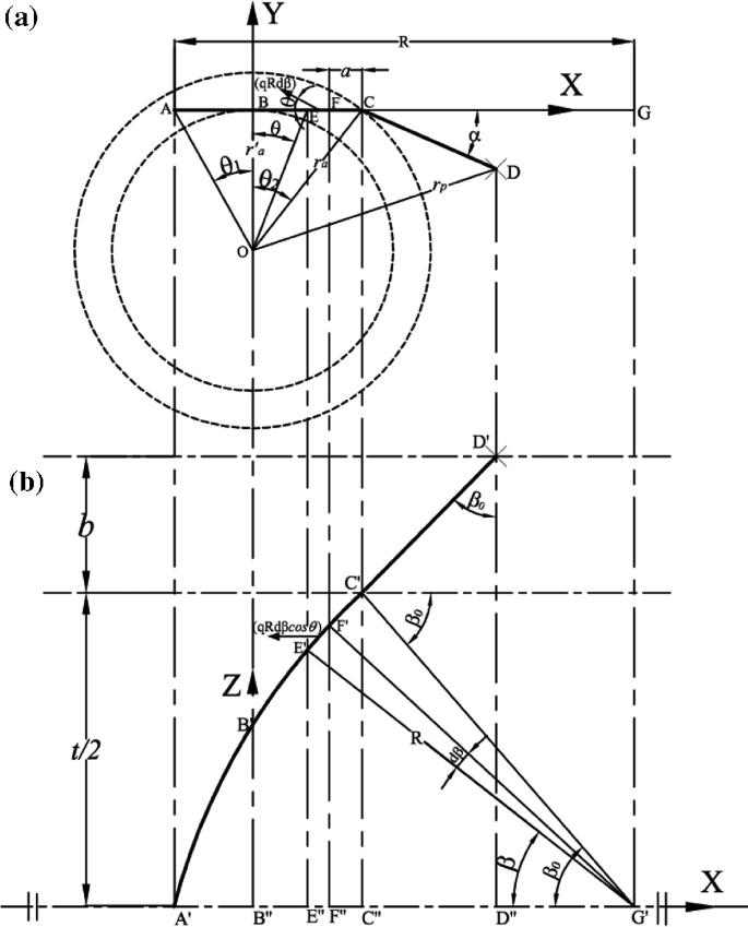
a Line diagram of wire for circular profile cutting (top view). b Line diagram of upper half of the wire for circular profile cutting (front view) [11]
-
(vi)
It is shown in Fig. 5a, b that gap force q applied on very tiny portion EF is qRdβ. This part of the gap force qRdβsinθ produces lateral bending on the EDM wire, and component qRdβcosθ applied in the same plane of wire profile creates bending. When job thickness (t) varies, θ also will vary, so the radius of curvature R will also simultaneously vary. Now, θ has very little value, so the variation of radius of curvature is neglected. It is also known that EDM wire may be treated as flexible wire.
-
(vii)
Generally, a small wire deflection occurred between the top and bottom job surfaces (δi), and when compared to the job thickness, the wire radius of curvature is typically very big. Therefore, it is assumed that β0 is small (Fig. 5b).


The X-, Y- and Z-axis are shown in Fig. 5a, b, and it is chosen in a way that origin is met at point B as it is the centre of the wire as shown in Fig. 5a and \(B^{\prime\prime }\) in Fig. 5b, and the cylindrical job axis is parallel to Z-axis. In Fig. 5a, \(r_{\text{a}}\) is the gap between cylindrical job centre and wire centre, and \(r_{\text{a}}^{\prime }\) is the shortest length between cylindrical job centre and wire centre. rw is radius of the wire, and \(\xi\) is the of radial overcut or radial spark gap.
The following expression may be written from Fig. 3;
where raj is the largest radius.
Cd′ is the wire position shown in Fig. 6 in the space, and it is above the job surface.

Location of wire on top of the workpiece surface in 3D spaces [11]
In Figs. 5a and 6, α is angle \(\angle DCG\). It is the projected value of wire inclination beyond the job surface on XY plane with regard to XZ plane, with respect to YZ plane \(\beta_{0}^{\prime }\) is exact inclination of the straight portion of the wire above the job surface (Fig. 6), this amount is identical to angle between wire guide and wire on XZ plane, and \(\beta_{0}\) is the projected value of \(\beta_{0}^{{\prime }}\) (Fig. 6). It is seen that if the value of α is small, C′D′ will be tangential to the curve A′C′, and so exact inclination of radius of curvature is also \(\beta_{0}\) at the point C (Fig. 5b).
CD is the wire position in XY plane, and CD′ is wire position in XZ plane top of the workpiece material. The following trigonometric relation is obtained from Fig. 6.
Now, dividing Eqs. (3) and (4), one can obtain the following expression
Putting the value of \(\frac{cd}{CD} = \cos \alpha\), the above equation becomes
Now, rearranging the above expression, it may be expressed as
Since α is very small, \(\cos \alpha \approx 1\) and \(\beta_{0}^{{\prime }} \;\& \;\beta_{ 0}\) are also small. Thus, the above expression becomes
In Fig. 6, \(Dd^{{\prime }} = b\) is the span between job surface and wire guide support, and the wire bending above the job surface and below the job surface δ0(=CD) is as shown in Fig. 7 and also can be expressed as follows

Wirelag phenomenon during circular profile cutting (top view) [11]
Hence,
Now, putting the value of \(\tan \beta_{0}^{{\prime }}\) from Eq. (8), it can be expressed as
Since α and \(\beta_{ 0}\) is small, the above expression becomes
From Fig. 5b, it is noticed that
As β0 is small, \({\sin} \beta_{0} \approx \beta_{0} \,\). Therefore, the radius of curvature R is expressed as
where t = thickness of the job.
From Fig. 5a, b, it is seen that
Putting the values of above expression in trigonometric form, it becomes
For small values of θ1, θ and β, \(\tan \theta_{1} \approx \theta_{1}\), \(\tan \theta \approx \theta\) and \(\cos \beta \approx 1 - \beta^{2} /2\), and the above expression becomes
Again rearranging, it becomes
Substituting the value of R from Eq. (15), the above expression may be evaluated as follows
Again from Fig. 5a, b, it is observed that \(a = FC = F^{\prime\prime } C^{\prime\prime }\), and a may be expressed as follows
If we consider only upper half of the wire, i.e., AC or A′C′, it is in equilibrium under the tensile force and the distributed gap force as shown in Fig. 5a, b. From the figure, it is seen that \(E^{\prime } F^{\prime }\) is a very small arc and it makes an angle dβ, and the radius of curvature R creates an angle β with negative X-axis. So, qRdβ is the gap force on this portion of the wire. So, the equilibrium equation may be written as
As radius of curvature R and gap force intensity q are considered as constant, as θ, α and β are small, \(\cos \theta \approx 1,\cos \alpha \approx 1\,{\text{and}}\,{\sin} \beta_{0}^{\prime } \approx \beta_{0}^{\prime }\), the above equation can be expressed as
Now, solving the above equation, it becomes
As it is obtained that \(\beta_{0}^{{\prime }} = \beta_{0}\), now, the above expression can be rewritten as
Combining Eqs. (15) and (24), \(\beta_{0}\) may be evaluated as follows:
Similarly, if equilibrium is considered along Y-axis, then the equation will be as
As the R and q are not changing, its value is fixed. For small values of θ, α and β, \(\sin \theta \approx \theta ,\sin \alpha \approx \alpha \;{\text{and}}\;\sin \beta_{0}^{\prime } \approx \beta_{0}^{\prime } \approx \beta_{0}\) and from Eq. (24), radius of curvature R = T/q. So, the above expression becomes
Putting the value of θ from Eq. (19), it becomes
Solving the above equation, it can be evaluated as
Now, rearranging the above equation, α becomes
Now, in the XY plane, it is seen from Fig. 5a that moment of the wire about point C will be zero. It may be expressed as
Now, putting the value of a from Eq. (20) and using \(\sin \theta \approx \theta\), the above expression becomes,
Since, \(qR^{2} \ne 0\),
Now, replacing the θ from Eq. (19) in the above equation, it becomes
After integrating between the limits, the above expression becomes
Rearranging the above equation, it may be expressed in terms of θ1 as follows
Now, putting the \(\theta_{1}\) value in Eq. (30), it becomes
From Fig. 5a, b, it is noticed that \(\theta = \theta_{ 2}\) and \(\beta = \beta_{0}\). So, using these limiting values of θ and β in Eq. (19), the expression becomes
Now, rearranging the above equation by putting \(\theta_{ 1}\), one can estimate the value of θ2 as given below:
In Fig. 7, considering ΔOCD, the following relationship is obtained
Putting the value of \(OC = r_{\text{a}} ,OC = r_{\text{a}} ,CD = b\beta_{0}\), the above expression becomes
Now, using α and \(\theta_{2}\) and Eqs. (37) and (39), respectively, the above expression becomes:
The value of \(\theta_{2}\) is small and as such \(r_{\text{a}}^{{\prime }} \approx r_{\text{a}}\); hence, the above expression becomes:
Putting the value of \(\beta_{0} = \frac{tq}{2T}\) using Eq. (25), the above equation may be expressed as
After rearranging the above equation, the gap force q can be calculated as below:
Substituting ra value as it is in Eq. (2), it becomes:
Now, \(\xi\) can be measured easily from a square or rectangular job and raj, and also we can get from a circular job which were cut from the job material for a given parameter setting. From the machining condition also we will get job thickness (t), wire tension (T), wire radius (rw) and the value of b. So, the average gap force intensity can be measured for any specified machining parameter setting using Eq. (46).
Now, using Eq. (43), ra may be expressed as follows:
Since, \(\beta_{ 0}\) is small, \(\beta_{ 0}^{{ 4 { }}}\) or higher order will be very small and can be neglected. So, the above equation becomes
After rearranging the above expression using the value of Eq. (25), it becomes
where
and
The right hand side of Eq. (49) will be constant for a specified machining parameter setting. So, the K is constant, and it is called radial wirelag compensation constant.
Now, wirelag compensation value \((\varepsilon_{\text{wl}} )\) can be measured for any radius circular or curved job using Eq. (52). This value is used in the CNC part program to get the accurate job dimension.
It is seen from Eq. (50) that smaller radius job will have higher imperfection though usually smaller radius job requires higher precision.
From Fig. 7, it is seen that CD is wire bending at the top surfaces of workpiece. The wire bending above the job surface δ0 can be evaluated by substituting the value β0 from Eq. (25) in Eq. (13) as follows:
Wire deflection or bending between top and below surface of the job in the direction of δ0 is HC = δi in Fig. 7. Hence, δi can be estimated as below:
For small values of θ1, θ2 and α, the above expression becomes
Now, putting the value of \(\theta_{1} + \theta_{2} = t\beta_{0} /4r_{\text{a}}^{{\prime }}\) from Eq. (38) and putting β0 value as in Eq. (25), it becomes
So, the total deflection δt
It is seen in the earlier research [2, 10] also that the same formula to measure wirelag or wire deflection when straight WEDM cutting was done.
It is already stated that a little amount lateral wire deflection is happening during machining. This deflection will be maximum at the middle length of the wire between upper and lower wire guide. Hence, the total lateral deflection at the middle portion of the wire length as shown in Fig. 7 is expressed as
For small values of θ1, θ2 and α, the above expression becomes
Now, putting the values of \(\theta_{1} + \theta_{2} = t\beta_{0} /4r_{\text{a}}^{{\prime }}\), α and β0 as in Eqs. (38), (37) and (25), respectively, and as at top and bottom surface wire deflection is same, then \(r_{\text{a}}^{{\prime }} \approx r_{\text{a}}\).
Hence, the expression for δl becomes
Now substituting ra value as in Eq. (2), the above expression may be rewritten as
It is seen from the above equation that lateral deflection is proportional with gap force and job thickness where as the wire tension and job radius (raj) is inversely proportional with lateral deflection. It is obvious that during straight profile cutting job, radius (raj) will be infinite. So, the lateral deflection will be zero. So, theoretically it proved that during straight profile cutting, no lateral deflection or bending occur.
4 Summary
To estimate gap force and wirelag, a new method is developed based upon the analytical model. Now, the wirelag value can be measured directly for any condition, and it can be used to produce accurate job. To increase the cylindrical or curved profile accuracy, the wirelag compensation value is incorporated in the CNC part program. From the investigation, it is clear that lower radius job is experienced higher wirelag. It is also shown that the lateral deflection is zero for straight profile cutting.
References
Dekeyser WL, Snoeys R (1989) Geometrical accuracy of wire-EDM. In: Proceedings of the international symposium for electro-machining, pp 226–232
Dauw DF, Beltrami I (1994) High-precision wire-EDM by online wire position control. Ann CIRP 43(1):193–197
Lin CT, Chung IF, Huang SY (2001) Improvement of machining accuracy by fuzzy logic at corner parts for wire-EDM. Fuzzy Sets Syst 122(3):499–511
Puri AB, Bhattacharyya B (2003) An analysis and optimisation of the geometrical inaccuracy due to wire lag phenomenon in WEDM. Int J Mach Tools Manuf 43(2):151–159
Dodun O, Gonçalves-Coelho AM, Slătineanu L, Nagîţ G (2009) Using wire electrical Discharge machining for improved corner cutting accuracy of thin parts. Int J Adv Manuf Technol 41:858–864
Sanchez JA, Lacalle LNLD, Lamikiz A (2004) A computer-aided system for the optimization of the accuracy of the wire electro-discharge machining process. Int J Comput Integr Manuf 17(5):413–420
Dauw DF, Sthioul H, Delpretti R, Tricarico C (1989) Wire analysis and control for precision EDM cutting. Ann CIRP 38(1):191–194
Lee TC, Yue TM, Lau WS (1997) The measurement and analysis of the wire vibration in ultrasonic aided wire cut machining. ICPE Taipei, Taiwan, pp 677–683
Mohri N, Yamada H, Furutani K, Narikiyo T, Magara T (1998) System Identification of Wire Electrical Discharge Machining. Annals of the CIRP 47(1):173–176
Beltrami I, Bertholds A, Dauw D (1996) A simplified post process for wire cut EDM. J Mater Process Technol 58(4):385–389
Sarkar S, Sekh M, Mitra S, Bhattacharyya B (2011) A novel method of determination of wire lag for enhanced profile accuracy in WEDM. Precis Eng 35:339–347
Author information
Authors and Affiliations
Corresponding author
Editor information
Editors and Affiliations
Rights and permissions
Copyright information
© 2020 Springer Nature Singapore Pte Ltd.
About this chapter

Cite this chapter
Sekh, M. (2020). Improvement of Profile Accuracy in WEDM—A Novel Technique. In: Kibria, G., Bhattacharyya, B. (eds) Accuracy Enhancement Technologies for Micromachining Processes. Lecture Notes in Mechanical Engineering. Springer, Singapore. https://doi.org/10.1007/978-981-15-2117-1_4
Download citation
DOI: https://doi.org/10.1007/978-981-15-2117-1_4
Published:
Publisher Name: Springer, Singapore
Print ISBN: 978-981-15-2116-4
Online ISBN: 978-981-15-2117-1
eBook Packages: EngineeringEngineering (R0)