
Abstract
This paper investigates the role of learning curve models in estimating construction productivity. Learning curve theory is actively implemented for both the scheduling and cost estimation of complex construction projects. The purpose of the research is to assess the suitability of published learning curve models in effectively analyzing the learning phenomenon for substantially complex construction operations. The research investigates five (5) learning curve models, namely the (a) Straight-line or Wright, (b) Stanford “B”, (c) Cubic, (d) Piecewise or Stepwise and (e) Exponential models. The methodology includes the comparative implementation of each one of the aforementioned models for the analysis of a large infrastructure project with the use of unit and cumulative productivity data. A two-stage investigative process for the five models was applied in order to define (a) the best-fit model for historical productivity data of completed construction activities and (b) the best predictor model of future performance. The assessment criterion for the suitability is the deviation of the real construction data from the predictions generated by each model. The research results indicate that the Cubic model dominates in terms of its predictive capability on historical data, while the Stanford “B” model is a better future performance predictor. Future research directions include the extension of the research scope with the inclusion of more learning curve models in conjunction with a populated database of historical field data.
Access provided by Autonomous University of Puebla. Download conference paper PDF
Keywords
1 Introduction
The estimation of construction productivity takes into account several factors that reflect the managerial perspective and philosophy of the project personnel (Panas and Pantouvakis 2010; Shan et al. 2011). One of the basic factors that affect productivity is the repetitive nature of construction activities. In view of this fact, the productivity improvement that is observed in subsequent production cycles of a specific repetitive construction process (e.g. high-rise building construction) is often attributed to the learning phenomenon that is developed in relation to the resources that are deployed in the project (Thomas et al. 1986; Pellegrino and Costantino 2018). In other words, the productivity of repetitive tasks is improved as the experience of the deployed crews is increased (Pellegrino et al. 2012). The required time (man-hours) for the completion of repetitive construction activities is decreased, as the repetitions increase, since (i) the crews are familiarized with the nature of the works, (ii) the coordination of the mechanical equipment and the crews is improved, (iii) the project management discipline is enhanced, (iv) more efficient techniques and construction methods are implemented, (v) more effective logistics management methods are followed and (vi) the project scope is narrowed, thus limiting the need for additional corrective activities (Thomas 2009). Within that framework, the learning phenomenon or learning curve effect expresses the influence of the human factor, namely the contribution of the deployed crews’ skill and experience in construction productivity.
The integration of the learning effect in construction productivity studies enhances the accuracy of time and cost management (Lutz et al. 1994), improves project control and programming (Pellegrino et al. 2012), as well as provides the required scientific evidence for claiming lost workhours (Thomas 2009). However, learning curve studies have also been criticized for having several limitations such as oversimplification of the construction process and implementation of a one-dimensional research approach where the analysis is based on a single learning model to interpret the actual data (Jarkas and Horner 2011; Jarkas 2016). More specifically, the vast majority of learning curve studies in construction uses the straight-line or Wright model, thus limiting the presented results’ scope and possibly ignoring the effect of other learning parameters on the investigated construction process. In that view, this research intends to conduct a comparative analysis of five (5) established and widely acceptable learning curve models with the intent to interpret a relatively complex construction process relating to the realization of a large-scale marine infrastructure project. The purpose is the examination of each model’s suitability to interpret historical productivity data and predict future performance, in order to provide project management executives with the necessary information to reach critical project decisions (e.g. increase/decrease of project resources deployment). It is, to the authors’ best knowledge, the first research attempt to investigate thoroughly the implementation of learning curve models in marine works from a productivity stance.
The structure of the paper is as follows: First, background information on pertinent research on learning curve theory is going to be provided, followed by a concise description of the construction process that served as the research testbed. Then, the research methodology is going to be delineated and, subsequently, the fitting results for the selected models will be presented. The main inferences emerging from the study will be described and, finally, the delineation of future research directions will conclude the study.
2 Background
2.1 Learning Curves
2.1.1 Theoretical Concepts
Learning curves are used for the graphical representation of the time span, the cost and/or the labour hours that are required for the execution of a series of “sufficiently complex” construction activities (Everett and Farghal 1994). The learning curve theory suggests that the required time (labour hours) for the production of a single unit (e.g. floor of a high-rise building) is incrementally decreasing as a percentage of the time that was demanded for the production of the previous unit (UN 1965; Jarkas and Horner 2011). This percentage is called “learning rate” and is a characteristic variable for the extent of the learning phenomenon in a single construction activity (Thomas et al. 1986). From a mathematical point of view, the learning rate coincides with the inclination of the learning curve. The smaller the value of the learning rate, the more intense the learning phenomenon, since each subsequent production cycle is a smaller percentage of the time required for the previous production cycle. For instance, when the learning rate equals 80%, then the required labour-hours for the production of a single unit is 20% less than the time needed for the production of the previous unit. If an activity presents a learning rate equal to 100%, then no learning phenomenon is developed for that specific task (Jarkas 2016).
The learning curve theory may be applied to the effort (typically measured in units of time) related to individual units or to the cumulative average time to complete a number of units (Farghal and Everett 1997; Jarkas and Horner 2011). If the first category of data is used, then the analysis is based on “unit data”, whereas when the second category of data is utilized the analysis falls under the “cumulative data” label. As to the latter, the cumulative average time is the average time required to install or complete a given number of units. It is computed by taking the total time required to install or construct a given number of units divided by the number of units completed (Hinze and Olbina 2009). Although in construction settings it is often most convenient to use the cumulative average time, this research adopts both types of data (unit and cumulative), in order to provide a more robust research framework. In terms of the applied analytical tools, most published research in learning curve productivity analysis adopts the statistical approach for the elaboration of field data (Thomas et al. 1986; Everett and Farghal 1997; Couto and Texeira 2005; Pellegrino et al. 2012; Ammar and Samy 2015; Srour et al. 2016), thus the same approach has been implemented in the current research as well. Regarding the projects’ scope for the implementation of learning curve theory, it ranges from concreting activities (Couto and Texeira 2005), to new buildings construction (Pellegrino et al. 2012) and reaching the realization of large-scale infrastructure works (Everett and Farghal 1997; Naresh and Jahren 1999).
2.1.2 Learning Curve Models
The learning curve phenomenon is studied through the use of specific mathematical models, which interpret the variation of productivity in relation to critical factors such as the number of units. There are five (5) main types of learning curve models whose concise description is as follows (Thomas et al. 1986; Everett and Farghal 1994):
-
Straight-Line Model (or Wright): It was first formulated by Wright in 1936 and is so named because it forms a straight line when plotted on a log-log scale (Lee et al. 2015). There are two types of Straight-line learning curve models which differ depending on either unit data or cumulative average are used. The underlying assumption of the model is that the learning rate (expressed as a percentage) remains constant throughout the duration of the activity (Thomas et al. 1986). The learning rate, L, can be derived from the slope of the logarithmic form by using L = 2−n, where n is the slope of the logarithmic curve (Srour et al. 2016). It is the most commonly used model in construction research (Jarkas 2016) because of its simplicity and its ability to provide acceptable precision (Srour et al. 2018).
-
Stanford “B” Model: It was developed, by the Stanford Research Institute in 1940’s. This model is considered a modified Straight-line model which includes a factor “B” to represent the number of units of prior experience and shifts the learning curve downward (Badiru 1992; Srour et al. 2016). It assumes that the Straight-line model is the normal situation provided the crew has no experience resulting from performing similar activities or constructing similar units in the immediate past. The value of “B” fluctuates within the range of 0–10 (Gottlieb and Haugbølle 2010; Mályusz and Pém 2014). A crew with no prior experience will have a value “B” equal with zero, while an experienced crew may have an experience factor of four or higher (Thomas et al. 1986).
-
Cubic Model: Carlson (1973) proposed the Cubic model and indicated that a further enhancement of the Straight-line model can be achieved using a curve with multiple slopes (Hijazi et al. 1992). This model assumes that the learning rate is not a constant variable because of the combined effects of previous experience and the levelling off of productivity as the activity nears completion. Factors “C” and “D” are estimated using the basic equation of the model and another data point along the curve.
-
Piecewise or Stepwise Model: It is a linearized approximation of the Cubic model with three distinct phases, while each one has a constant learning rate. On a log-log plot, this model appears as three straight line segments with different slopes. As seen on Fig. 1 the first segment represents the operation-learning phase, while the second segment starts at point xp1 and denotes the phase where the learning phenomenon develops. The third segment initiates at point xp2 and represents the end of the routine-acquiring phase. Hence, this point is also called the “standard production point” as no significant further improvement of productivity is observed beyond that point (Thomas et al. 1986).
Fig. 1 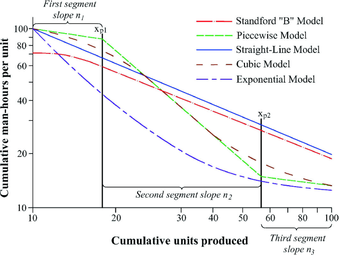
(adopted from Thomas et al. 1986)
Shape of various learning curve models
-
Exponential Model: It was developed by the Norwegian Building Research Institute in 1960 (U.N. 1965). It is based upon the rule that part of time/cost per unit is fixed and the other part of time/cost per unit, which can be reduced by repetition, will be reduced by one-half after a constant number of repetitions (Zahran et al. 2016). The ultimate or lowest cost or man-hours or time per unit at the end of the routine-acquiring phase (Yult) must be known along with constant “H” which represents a “Halving Factor”, namely the number of units required for that part of the unit cost which can be reduced by repetition to one-half. A learning curve model for cumulative data was not presented (Thomas et al. 1986).

The mathematical expressions for the estimation of productivity based on the aforementioned learning curve models (LC models) are summarized in Table 1 and their graphical representation is depicted in Fig. 1.
2.2 Caisson Construction Operations
In general, floating caissons are prefabricated concrete box-like elements with rectangular cells that are suited for marine and harbor projects and are usually cast on floating dry docks (Panas and Pantouvakis 2014). Due to the standardized shape of the caissons and the repetitive nature of the works, since caissons are always constructed in batches, the concreting process is most commonly executed with the use of the slipforming construction technique. Slipform is a sliding-form construction method, which is used to construct vertical concrete structures (Zayed et al. 2008). Generally, the concreting and slipforming process comprises three sub-phases (see Fig. 2): (i) slipform assembling phase, (ii) slipforming phase (including an initial concreting phase) and (iii) slipform dismantling phase. Although Pantouvakis and Panas (2013) identified nineteen activities for the construction of a caisson, this study focuses only on the aforementioned activities, because a fundamental prerequisite for the learning phenomenon to develop is for productivity improvements to be able to occur as a result from repeating “sufficiently complex” activities (Thomas 2009). As such, in the case of caissons construction operations, only these activities were found to inherently possess such characteristics, since the observed productivity of the other activities did not fluctuate significantly during the construction phase. For space limitation reasons, the total caisson construction process is going to be analyzed in this paper with no particular focus on individual activities.

Floating caisson production cycle
3 Research Methodology
A large-scale marine project served as the case study for the current research. The project was completed in 2012 and comprised the construction of 34 caissons (Panas and Pantouvakis 2018). A two-stage investigative process for the five learning curve models was applied in order to define (a) the best-fit model for historical productivity data of completed construction activities and (b) the best predictor model of future performance (Everett and Farghal 1994). The solver function of MS Excel (version 2010) has been used in conjunction with the least squares method, so as to determine the optimum learning curve models parameters.
-
Stage Α: Assessment of Best Fit Model with Historical Productivity Data
The analysis is conducted for both unit and cumulative data. The least square method is used in order to determine the optimum fitting curve. Pearson’s coefficient of determination (R2) is the preferred metric for the evaluation of each model’s robustness and fluctuates from 0 to 1.00. The closer the R2 values to 1.00, the better the correlation of the fitted data to the selected model.
-
Stage Β: Assessment of Best Prediction Model for Future Performance
The analysis is confined to the unit data. As proposed by Everett and Farghal (1994), productivity data are divided in half, so as for the first 17 caissons to become the “historical data” and the next 17 caissons to be the future data. As before, the least squares method is used in conjunction with the Pearson’s coefficient of determination for the estimation of the first 17 caissons (R21–17). Subsequently, the computed learning curves (1–17 caissons) are extended from the 17th to the 34th caisson. Taking into account that Pearson’s coefficient of determination (R2) is not valid for correlating points with best-fit curves outside the range of points used to determine the best-fit curve, a new metric is used as follows (Everett and Farghal 1994):
where: m = the number of caissons to be fitted; k = the number of caissons to be predicted, \({\text{y}}^{{\prime }}_{{{\text{m}} + {\text{i}}}}\) = the value found on the extension of the best-fit curve; ym+i = the actual measured values; Ef = average percentage error, which ranges from 0% indicating a perfect correlation between the extended best-fit curve and the actual data to large positive values indicating no correlation.
4 Results
-
Stage Α: Assessment of Best Fit Model with Historical Productivity Data
Table 2 summarizes each model’s performance, while Figs. 3 and 4 give a graphical representation of the results. There is a clear indication that the Cubic model demonstrates the best fitting results for unit data relating to the total caisson construction process. The Exponential model gives the least favorable adjustment, without being unacceptable, though, in absolute terms. These results enhance previous research and denote that the best fit model depends on the location and the nature of each project. For the cumulative data, again the Cubic model gives the best predictions. In fact, the cubic learning curve almost coincides with the real data. The other three models give a correlation coefficient very close to 1.00 which denotes a generally satisfactory prediction capability for all learning curve models.

Learning curves for historical data (Unit)

Learning curves for historical data (Cumulative)
In principle, the correlations for the cumulative data are better than the equivalent ones for the unit data, since the former give a more smooth graphical representation of the learning phenomenon. Comparing the Cubic and Piecewise models with the Straight-line model for the unit data there is a practically insignificant difference of 2.51% and 0.43% respectively (p < 5%). The same results for the cumulative data range at the amount of 1.96% and 0.05% respectively (p < 5%). This fact corroborates the tendency of the construction industry to characterize the Straight-line model as more “user-friendly” since (a) it yields similar results with the other LC models, (b) is much simpler in its implementation in terms of the required input data and parameters and (c) less assumptions are needed to be made.
-
Stage Β: Assessment of Best Prediction Model for future performance
As depicted in Table 3, the best prediction model for future performance based on unit data is Stanford “B”, since the average percentage error has a value of Εf(18–34) = 5.7%, which denotes good correlation between actual data and the extended curve. It is generally acceptable that Stanford “B” model simulates with acceptable accuracy complex construction processes, especially in large-scale projects. A graphical representation of the learning curve models’ predictions is depicted in Fig. 5. The results for the Cubic and Piecewise models verify the findings of Everett and Farghal (1994), who claimed that these models are not a good predictor for future activities. More specifically, the Cubic model has the best value for R2(1–17), but also presents the largest error margin of Ef(18–34) = 17.42. Also note in Fig. 5, that the extension line of the Cubic model seems to increase significantly beyond the 25th caisson. A similar, but opposite trend is found for the Piecewise model as well, while it presents fairly equivalent error value (Ef(18–34) = 16.21). Although, both models appear to be a reasonable predictor, these models deviate from the actual data for long-term prediction, since the extended curves continue upward or downward towards unrealistic values.

Learning curves and learning curves extensions of models for unit data
5 Conclusions
The conducted research demonstrated that the learning effect was intensely present in the studied project, which resulted in significant improvements in caissons construction productivity. All five (5) learning curve models were scrutinized for unit and cumulative historical productivity data and yielded a coefficient of R2 > 0.90, which denotes a strong correlation to real data. The Cubic model has proven to be the best performer in terms of its adjustment capability to the historical data.
In terms of the future performance prediction capability, unit data was solely used for all learning curve models. Stanford “B” model was found to be the best predictor, with the Exponential and Straight-line model being quite close in terms of predictability. Therefore, it is beyond doubt that learning curve theory is an efficient and effective tool for assessing historical and predicting future productivity data in the case of caisson construction operations.
Possible research extensions could be developed in the area of future performance predictions, by adopting different data representation techniques such as (a) cumulative average data, (b) moving average data and (c) exponential weighted average. The research scope may be enhanced with the inclusion of other (non-classic) learning curve models (e.g. DeJong, Knecht, hyperbolic models), which were excluded from the current study due to brevity reasons. The enhancement of the already established historical project database with even more data covering similar activities is deemed necessary, so as to be able to structure a future performance prediction tool with inherent flexibility to simulate different work scenarios and feed project executives with valuable insights for informed decision making.
References
Ammar MA, Samy M (2015) Learning curve modelling of gas pipeline construction in Egypt. Int J Constr Manag 15(3):229–238
Badiru AB (1992) Computational survey of univariate and multivariate learning curve models. IEEE Trans Eng Manage 39(2):176–188
Carlson J (1973) Cubic learning curves: precision tool for labor estimating. Manuf Eng Manag 67(11):22–25
Couto JP, Teixeira JC (2005) Using linear model for learning curve effect on highrise floor construction. Constr Manag Econ 23(4):355–364
Everett JG, Farghal S (1994) Learning curve predictors for construction field operations. J Constr Eng Manag 120(3):603–616
Everett JG, Farghal S (1997) Data representation for predicting performance with learning curves. J Constr Eng Manag 123(1):46–52
Farghal S, Everett JG (1997) Learning curves: accuracy in predicting future performance. J Constr Eng Manag 123(1):41–45
Gottlieb SC, Haugbølle K (2010) The repetition effect in building and construction works. Danish Building Research Institute, Kobenhaven
Hijazi AM, AbouRizk SM, Halpin DW (1992) Modeling and simulating learning development in construction. J Constr Eng Manag 118(4):685–700
Hinze J, Olbina S (2009) Empirical analysis of the learning curve principle in prestressed concrete piles. J Constr Eng Manag 135(5):425–431
Jarkas A (2016) Learning effect on labour productivity of repetitive concrete masonry blockwork: Fact or fable? Int J Prod Perform Manag 65(8):1075–1090
Jarkas A, Horner M (2011) Revisiting the applicability of learning curve theory to formwork labour productivity. Constr Manag Econ 29(5):483–493
Lee B, Lee H, Park M, Kim H (2015) Influence factors of learning-curve effect in high-rise building constructions. J Constr Eng Manag 141(8):04015019
Lutz JD, Halpin DW, Wilson JR (1994) Simulation of learning development in repetitive construction. J Constr Eng Manag 120(4):753–773
Mályusz L, Pém A (2014) Predicting future performance by learning curves. Procedia-Soc Behav Sci 119:368–376
Naresh AL, Jahren CT (1999) Learning outcomes from construction simulation modeling. Civ Eng Environ Syst 16(2):129–144
Panas A, Pantouvakis JP (2010) Evaluating research methodology in construction productivity studies. Built Hum Environ Rev 3(1):63–85
Panas A, Pantouvakis JP (2014) Simulation-based and statistical analysis of the learning effect in floating caisson construction operations. J Constr Eng Manag 140(1):04013033
Panas A, Pantouvakis JP (2018) On the use of learning curves for the estimation of construction productivity. Int J Constr Manag. https://doi.org/10.1080/15623599.2017.1326302
Pantouvakis JP, Panas A (2013) Computer simulation and analysis framework for floating caisson construction operations. Autom Constr 36:196–207
Pellegrino R, Costantino N (2018) An empirical investigation of the learning effect in concrete operations. Eng Constr Archit Manag 25(3):342–357
Pellegrino R, Costantino N, Pietroforte R, Sancilio S (2012) Construction of multistorey concrete structures in Italy: patterns of productivity and learning curves. Constr Manag Econ 30(2):103–115
Shan Y, Goodrum PM, Zhai D, Haas C, Caldas CH (2011) The impact of management practices on mechanical construction productivity. Constr Manag Econ 29(3):305–316
Srour FJ, Kiomjian D, Srour IM (2016) Learning curves in construction: a critical review and new model. J Constr Eng Manag 142:06015004
Srour FJ, Kiomjian D, Srour IM (2018) Automating the use of learning curve models in construction task duration estimates. J Constr Eng Manag 144(7):04018055
Thomas HR (2009) Construction learning curves. Pract Period Struct Des Constr 14(1):14–20
Thomas HR, Mathews CT, Ward JG (1986) Learning curve models of construction productivity. J Constr Eng Manag 112(2):245–259
United Nations Committee on Housing Building and Planning (1965) Effect of repetition on building operations and processes on site. United Nations, New York
Zahran K, Nour M, Hosny O (2016) The effect of learning on line of balance scheduling: obstacles and potentials. Int J Eng Sci Comput 6(4):3831–3841
Zayed T, Sharifi MR, Baciu S, Amer M (2008) Slip-form application to concrete structures. J Constr Eng Manag 134:157–168
Author information
Authors and Affiliations
Corresponding author
Editor information
Editors and Affiliations
Rights and permissions
Copyright information
© 2020 Springer Nature Singapore Pte Ltd.
About this paper

Cite this paper
Ralli, P., Panas, A., Pantouvakis, JP., Karagiannakidis, D. (2020). Comparative Evaluation of Learning Curve Models for Construction Productivity Analysis. In: Panuwatwanich, K., Ko, CH. (eds) The 10th International Conference on Engineering, Project, and Production Management . Lecture Notes in Mechanical Engineering. Springer, Singapore. https://doi.org/10.1007/978-981-15-1910-9_29
Download citation
DOI: https://doi.org/10.1007/978-981-15-1910-9_29
Published:
Publisher Name: Springer, Singapore
Print ISBN: 978-981-15-1909-3
Online ISBN: 978-981-15-1910-9
eBook Packages: EngineeringEngineering (R0)