Performance Optimization of Applications

Abstract

In this chapter, we present procedures for performance evaluation that we have used for practical applications. The method is outlined in Sect. 2.1, and Sects. 2.2–2.6 describe the details of the method. The classification of problems related to high parallelism and the classification of applications from the viewpoint of single-CPU performance are described. Sections 2.7 and 2.8 then describe performance optimization techniques for each problem pattern related to high parallelism and the techniques for single-CPU performance optimization according to application classification.

2.1 Performance Evaluation Method

The performance evaluation of an application is divided into two parts: “highly parallel performance optimization” and “single-CPU performance optimization.” For each part, the performance evaluation method has two working phases: “current state recognition” and “understanding the problems.” The “current state recognition” is common to both working phases and is divided into “source code investigation” for analyzing the structure of source code, and “measurement of elapsed time” to understand the current state of application performance. The final procedure in the “current state recognition” is “calculation/communication kernel analysis,” in which we evaluate the results of “source code investigation” and “measurement of elapsed time.” The next phase of “current state recognition” begins with “problem evaluation method” with working phases of “understanding the problems.” In the “problem evaluation method” for “highly parallel performance optimization,” the problems related to high parallelization are classified into six patterns. In the “problem evaluation method” for “single-CPU performance optimization,” applications are also classified into six patterns.

Our approach is summarized in Table 2.1.

Table 2.1 Outline of performance optimization method

2.2 Current State Recognition: Source Code Investigation

As the first step in current state recognition, we investigate the source code of the application. We investigate the structure of the source code and analyze the call structure of subroutines and functions. We also analyze the subroutines, the loop structure in the functions, and the control structure of the IF blocks, and organize and visualize the structure of the entire program. The visualized source code is divided into blocks of calculation and communication processing according to the algorithms of physics and mathematics used in the program, and the blocks are organized. We understand the physical/mathematical processing content of each processing block . By comparing these aspects of the processing blocks with the results of the investigated source code, the calculation characteristics for each calculation block are obtained. The calculation characteristics describe the processing of a calculation block as nonparallel, completely parallel, or partially parallel, and identify the calculation index (e.g., number of atoms or number of meshes), whether the calculation amount in the calculation block is proportional to N or proportional to N² when the calculation index is N, and so on. We also investigate the communication characteristics of each communication block : whether the processing of the communication block is global communication , adjacent communication , or whether the communication amount depends on the calculation index. These investigations are shown in Fig. 2.1.

Fig. 2.1

Investigation of source code

The purpose of the investigation of the source code is to understand the characteristics of each processing block in the program. However, the visualization of the loop structure from the start to the end of the program and that of the entire control structure of the IF blocks mentioned here are large tasks if done manually. Therefore, we use a visualization tool for program structure, such as K-scope [1, 2].

2.3 Current State Recognition: Measurement Methods

In the sequential calculation before parallelization in the simulation, the calculation is sequentially performed for each calculation unit such as a mesh. To parallelize a code, we divide a set of calculation units such as meshes into plurality sets, share the divided sets among the processors, and perform the calculations in parallel. In such parallel computation, adjacent communications are performed in every calculation step to exchange data for parts of areas with neighboring processors. In addition, when calculating inner products of scalar values for all areas, global communication between all processors is required. An important point in achieving high parallelism is to make the adjacent and global communication times as small as possible.

As described in Sect. 1.2.1, it is important in parallel computation, just like the reduction of communication time, to make the nonparallel computing parts as small as possible.

The next step of current status recognition is to conduct application performance measurement. It is important for these measurements to be useful for investigating parallel characteristics; that is, what kind of behaviors the adjacent and global communication times described here show during highly parallel calculation, and where nonparallel computing parts remain and their influence on behaviors in high parallelism. Therefore, where performance measurement is possible, it is carried out as follows.

In conducting application performance measurement as the next step of current status recognition, it is important to conduct performance measurements that clarify the parallel characteristics of applications: specifically, what kind of behaviors the adjacent global communication times display during the highly parallel calculation, which calculation parts are nonparallel, and how the nonparallel parts influence the application’s behavior in highly parallel execution. For clarification of parallel characteristics, where possible, the performance measurement is carried out as follows.

First, we define the problem to be solved, determine the number of parallel paths in the problem, and create a test problem that has the same problem size with one processor as the target problem that can be run with several levels of parallelism. Next, we perform the performance measurement using the prepared test problem. In the performance measurement, the execution time is measured for each process for each calculation block and communication block , as defined in the previous section. The parallel characteristics during parallel computation cannot be fully clarified by measuring the entire application. Each processing block’s influence on the parallel characteristics differs depending on whether it includes a nonparallel part and the number of parallel paths, and whether the communication time changes. Therefore, it is essential to measure the performance of each processing block for each process separately. These measurements allow us to identify the processing blocks that degrade parallel performance. In addition, because the communication behavior during parallel execution differs between adjacent and global communication , it is necessary to measure them separately. The adjacent communication time has the same value if the communication amount is the same, as described later, but the global communication time tends to increase as the number of parallel paths increases, even if the communication volume stays the same. Furthermore, because communication times may include waiting times caused by load imbalance , it is also important to measure the waiting time and the net communication time separately, thus allowing us to distinguish whether the problem is caused by communication or load imbalance . With respect to computation, simultaneously with the computation time, the amount of computation and the computation performance are also measured for each processing block in each process.

2.4 Current State Recognition: Determination of Computation and Communication Kernels

The analysis of the source code shows the correspondence between the physical/mathematical processing contents of each processing block and the source code, and the calculation characteristics of each calculation block and the communication characteristics of each communication block . By matching these results with measurement results, the calculation kernel and the communication kernel can be identified.

For example, suppose there is a parameter N that determines the amount of computation. Assume that the coefficient of computation amount proportional to the third power of N is m1, the coefficient of computation amount proportional to N is m2, and that m2 is considerably larger than m1. When N is relatively small, the amount of computation for the two parts may be about the same. However, as N increases, the amount of computation for the part proportional to the third power of N becomes significantly larger, and the amount of computation for the part proportional to N may become negligible.

Both the amount of computation and the computation time also vary depending on the level of performance¹ that can be obtained relative to the theoretical peak performance . The essentially nonparallel parts may remain because of the adopted parallelization method. By considering the size of the parameters of the problem to be solved in this way, the parallelization method used, the parallelization method that may be adopted in the future, the prospects for effective performance, and so on, and the kernels to be evaluated, are determined (see Fig. 2.2). The kernels selected here can be reviewed at later stages of the evaluation.

Fig. 2.2

Identifying kernel of calculation and communication

2.5 Understanding the Problems: Evaluation of High-Parallelism Problems

We explain how to evaluate the problems of high parallelism by carrying out the measurements shown in Sect. 2.3 and how to measure parallel performance from several parallel processes to about 100, about 1000, or several thousand, step by step. There are two kinds of methods for measuring the performance by gradually increasing the number of parallel processes: strong scaling measurement and weak scaling measurement. Strong scaling measurement is a method of fixing the scale of the problem to be solved and increasing the number of parallel processes: for example, if the problem scale is fixed to N = 10,000, the number of parallel processes and the problem size per processor change is 1 and 10,000, 2 and 5000, 4 and 2500, and so on, respectively. In contrast, weak scaling measurement is a method of fixing the scale of the problem solved by each processor and increasing the number of parallel processes. For example, if the problem scale is measured first at N = 1000, the problem size per processor and the number of parallel processes is 1000 and 2, respectively, and the total problem scale is N = 2000. If the problem scale per processor and the number of parallel processes is 1000 and 4, the total problem scale is increased to N = 4000. The feature of weak scaling measurement is, ideally, that even when the number of parallel processes is increased, because the same computation is performed, and the adjacent communication amount is not changed, the execution time of the computation parts and the execution time of the adjacent communications are not changed. When a nonparallel part is included in the computation part, a significant increase in computation time should be measured, as the number of parallel processes becomes large in weak scaling measurement.

For example, assume that the execution time of the parallelizable part during sequential execution is T_p and the execution time of the nonparallelizable part during sequential execution is T_s. The execution time T₀ during sequential execution is represented by T₀ = T_p + T_s. The execution time when this problem is multiplied by N and executed sequentially is represented by N × T₀ = N × T_p + N × T_s. When this problem is executed in N parallel processes, it corresponds to what we performed with weak scaling . If the execution time when executed in N parallel processes is T_wn, the parallelizable portion becomes N times faster but the nonparallelizable portion does not become faster, so T_wn = T_p + N × T_s, and the term N × T_s increases. Incidentally, if T_sn is the execution time when run with strong scaling , then T_sn = T_s + T_p/N.

Even when the adjacent communication time increases in accordance with the number of parallel processes, it is easy to see that there are some problems in the corresponding adjacent communications . The global communication time generally increases in accordance with the number of parallel processes, and the increase can be predicted from the data on the basic communication performance by comparing the degree of increase with the predicted value. This can show whether there are some problems in the corresponding global communications .

The method described here is shown in Fig. 2.3. The reason for using weak scaling measurement in this way is that it is easy to find problems. However, in weak scaling measurement, it is necessary to prepare separate execution data according to the number of parallel processes, which may be troublesome. In a simulation in which the amount of computation is proportional to the second or third power of the problem size N, weak scaling measurement is sometimes difficult. In such a case, strong scaling measurement is performed. For strong scaling measurement, it is necessary to model the computation and communication times with the number of parallel processes as a parameter, to predict these, and to compare the predictions with the actual measured times so as to find any nonparallel parts or communication problems. However, unlike weak scaling measurement, it is not necessary to prepare execution data according to the number of parallel processes. It is sufficient to prepare only one type of data.

Fig. 2.3

Measurement with weak scaling

For the calculation of kernel, we compare and evaluate the trend of the predicted computation amount as clarified in the investigation of the source code and the computation amounts from the measurement results. For example, assume the computational amount of the kernel is proportional to the problem size N and is completely parallelized and measured with weak scaling . Because the computational amount for each process is constant regardless of the number of parallel processes, the calculation time for the total system is constant. In this case, the value obtained by dividing the computational amount of the measurement result by N is the proportional coefficient. If it can be evaluated with weak scaling , as described above, and if it is possible to completely parallelize and there are no problems in the communication part, even if the number of parallel processes is increased, the execution time of the computation part will be constant, and the adjacent communication time will also be constant and should not increase. If the execution time of the computation part increases remarkably with the number of parallel processes, it is likely that some nonparallel parts remain in the operation kernel. In addition, if the adjacent communication time increases significantly according to the number of parallels, it is likely that some processing that is not adjacent communication is included in the communication kernel. For example, there may be some global communication that is used instead of adjacent communication to simplify programming. As for the global communication , as described at the beginning of this section, its communication time also increases as the number of parallel processes increases. However, because the extent of the increase can be predicted from the basic communication performance data, if the communication time increases significantly more than predicted, we can consider that there is some problem in the corresponding global communication . In the discussion of measurement methods, we described the method of measuring the communication time and waiting time separately. This measured waiting time often indicates some imbalance included in the computation part and communication part.

In parallel computing, some processing imbalance is physically unavoidable. However, where the extent of the imbalance is remarkably large or if the imbalance increases with the number of parallel processes, it is likely that some problem causing imbalance was introduced in the programming stage. In evaluations using strong scaling , as described above, the existence of nonparallel parts and communication problems are found by comparing the predicted computation and communication times with the measured times. The predicted times are obtained by modeling them with the parallel number N as a parameter.

For example, suppose that the computation of the kernel is proportional to the third power of the system parameter N and the computation kernel is completely parallelized. When measured with strong scaling , if the number of parallel processes is doubled, then the computation of each process should be halved.

The total computation amount is the number of processes multiplied by the measured computational amount of each process and the parallel number M. The total computational amount divided by the third power of M is the proportional coefficient for the third power of M. The investigation of these computational amounts and proportional coefficients is performed using many parallel measurement results, and the evaluation is made as to whether the predicted value is consistent with the measurement results. If the evaluation results are consistent, it means that the source code is written according to the theory. If the evaluation results are not consistent and there is an increase in computational amounts with the increase in the number of parallel processes, it is likely that there is some problem such as the existence of nonparallel parts in the source code. A similar evaluation is required for the adjacent communications . For example, when a rectangular parallelepiped area is calculated using twice the number of parallel processes, the length of one side of the allocated area of each processor is 1/3 to the power of 1/2. The adjacent communication amount for the adjacent faces is 2/3 to the power of 1/2. Therefore, assuming the same communication performance, the communication time should also be 2/3 to the power of 1/2. For the global communication , a similarly modeled evaluation is required. As for the evaluation of the imbalance, it is necessary to evaluate the results as for weak scaling .

As repeatedly described, it is essential to carry out the evaluation shown here for each computation and communication kernel. Some tools provided by manufacturers have functions to measure the execution time, the amount of computation, and the computation performance for each subroutine or function, and it is usual to measure performance using these tools. However, the subroutines and the functions of the application do not generally match the range of the block, and because a function may be called from different blocks several times in different ways, these tools may not yield accurate measurement results for each block. Therefore, it is better to perform measurements on each block. However, this does not apply if the subroutine or function is configured to match the block.

2.5.1 Classification of Problems Related to High Parallelism

In the HPCC benchmark, applications are classified by using two axes. The first axis is defined by the locality versus nonlocality in the spatial direction of the data divided among the processors. The second axis is defined by the locality versus nonlocality in the temporal direction of data in the processors [3].

In addition, a study of application classification, the “Berkeley 13 dwarfs,” classified applications by the two axes of the communication and calculation patterns [4]. In this study, applications were classified among seven dwarfs in the HPC field, and 13 dwarfs by adding other fields.

In promoting performance optimization, we also classify the application and organize the execution performance optimization methods for applications based on the classification. For high parallelism, the locality versus nonlocality of the data is considered in the HPCC as one axis, and in the Berkeley 13 dwarfs, the pattern of communication is considered as one axis. In this section, we focus on the kinds of problems that occur and how we deal with those problems when optimizing the performance of existing applications, and we classify them according to highly parallel patterns. The problems relating to high parallelism are classified into six patterns, as shown in Table 2.2.

Table 2.2 Bottlenecks in parallel performance

The main problems relating to high parallelism are caused by calculations and communication. The first, second, and sixth problems are caused by calculation, and the third, fourth, and fifth problems are caused by communication. The six patterns are described as follows.

The first pattern is the mismatch of the degree of parallelism between applications and hardware. Researchers want to solve a problem within a certain time; suppose that to do so, it is necessary to use tens of thousands of parallel nodes on a supercomputer. For example, the K computer makes it possible to use more than 80,000 parallel nodes in terms of parallelism of the hardware. However, sometimes only thousands of parallel nodes can be used because of the limitations of the application parallelization. This is the mismatch of degree of parallelism between the application and the hardware. When approaching the limitation of the parallelism of the application, the computation time becomes extremely small, whereas the proportion of communication time increases, leading to a deterioration of the parallel efficiency .

The second pattern is the presence of nonparallel parts. As mentioned at the beginning of this chapter, we can see that the parallel performance deteriorates because of Amdahl’s law if nonparallel parts remain in the computation. Here, assuming that the execution time of a certain application at the time of sequential execution is T_s and the parallelization rate of the application is α, the nonparallelization ratio of the application is 1 – α. When this application is executed using n parallel processes, the execution time T_n is expressed as T_n = T_s (α/n + (1 – α)). For a parallelization efficiency of 50%, the parallelization ratio α is required to be 99.99% when n = 10,000. The easiest way to find remaining nonparallel parts is to measure the increase in execution time of the calculation part using weak scaling measurement as described above.

The third pattern is the occurrence of large communication sizes and frequent global communication . Communication times, particularly for global communications , have a large impact on the parallel performance. Consider an example of implementing the ALLREDUCE communication of M (bytes) between N nodes. Assume that the ALLREDUCE communication is performed using a binary tree algorithm and the communication performance is P_t (bytes/s). The communication time T_g for acquiring the total amount of M (bytes) after all nodes have communicated is $T_{g} = \frac{{m \times \log_{2} n}}{{P_{t} }}$. To compare the global communications with the adjacent communications , we consider an example in which N nodes perform the adjacent communications of M (bytes) to the next rank. When the communication performance is matched with the above conditions, the communication time T_a to complete the communication of M (bytes) for all nodes is calculated by $T_{a} = \frac{m}{{P_{t} }}$. When comparing global and adjacent communications , it is found that the global communication time is larger by the coefficient of $\log_{2} {\text{n}}$. Global communication should be a minimum.

The fourth pattern is the occurrence of global communications among all nodes. As described above, when the ALLREDUCE communication of M (bytes) is performed between N nodes using the binary tree algorithm, the communication time T is ${\text{T}} = \frac{{m \times \log_{2} n}}{{P_{t} }}$ assuming the communication performance to be P_t (bytes/s). Because the communication time increases as the number of nodes N increases, it is better to limit global communication among all nodes as much as possible. However, calculation of inner products is inevitable in the iterative solution of simultaneous linear equations and other problems, so it is impossible to eliminate all-node global communication .

The fifth pattern is the occurrence of a large communication size and a large number of communications in the adjacent communication . In terms of the communication time, adjacent communication tends to be faster than global communication . However, useless adjacent communication , such as communicating data for the entire area for one mesh to the adjacent mesh, are sometimes performed. Such code should be reviewed and only communication of data on the adjacent surface should be made.

The sixth pattern is the occurrence of load imbalances . Differences in the amount of calculation for each node may occur, causing some load imbalance among nodes. When the load imbalance deteriorates as the number of nodes increases, or when the load imbalance is extremely large over a small number of nodes, it is a problem.

2.6 Understanding the Problems: Evaluation Methods for Problems in Single-CPU Performance

2.6.1 Application Classification for Single-CPU Performance

As mentioned in Sect. 2.5, the developers of the HPCC benchmark [3] and the Berkeley 13 dwarfs [4] classified applications. For the HPCC, applications were classified using locality versus nonlocality of data in the temporal direction with regard to the single-CPU performance. For the Berkeley 13 dwarfs, applications were classified using the calculation pattern.

Similarly, in promoting the study of performance optimization, we also classify applications and organize the application execution performance optimization techniques based on the classification. In Sect. 1.2, from the viewpoint of the single-CPU performance, we mentioned that applications can roughly be classified into two types, one with a low required B/F value and one with a high required B/F value . This idea is close to the classification used for the HPCC. In this section, we will develop this view and show the classification of applications into six types as shown in Table 2.3.

Table 2.3 Classification of applications from the standpoint of single-CPU performance

The calculations for which the required B/F value is small are the first to the fourth types. The performance greatly varies depending on whether the DGEMM library or manual cache blocking can be used, even for calculations with small required B/F values . When cache blocking can be used, the performance varies depending on whether the data structure and loop structure are simple, or the data structure is slightly complicated such as using list vector indexing by integer arrays. Applications with more complex loop structures often fail to achieve high performance. These considerations led to the four types of calculations with small required B/F values .

The first type includes applications that can be rewritten as matrix–matrix product calculations. This type has small B/F values because in principle it can perform the calculations proportional to the third power of n by loading the data for a square of size n from memory. An example of this type of calculation is the application of the first principle quantum calculation based on density functional theory .

The second type includes applications that allow cache blocking although they are not rewritable to the matrix–matrix product , but still have small required B/F values . The calculation of the Coulomb interactions of molecular dynamics and the calculation of the gravity interaction of the gravitational multiple-body problem are examples. In both cases, by loading the data for n particles and performing cache blocking , calculations proportional to the square of n can be performed, so that the required B/F value is small. This type often uses list vector indexing by integer arrays for the particle access, and the loop body² is somewhat complicated.

The third type contains examples such as special high-precision stencil calculations,³ which make it possible to use the cache effectively, so the required B/F value is small and the loop body is a simple calculation. Although this type of calculation gives good performance, unfortunately there are few examples.

In the fourth type of calculations, the required B/F value is small, but the loop body is complex. Some weather calculations have mechanical processes to calculate the motion of a fluid and physical processes to calculate the microphysics of clouds; this physical process corresponds to the fourth type of calculation. By using small amounts of data loaded from the memory, complex and in-cache calculations are performed, but the loop body tends to be long and complicated. The calculation of the PIC method⁴ used for plasma calculations is also of this type. In this technique, although the mesh data around the particle are cached , list vector indexing by integer array is commonly used to access the particle data, resulting in complex program codes. The body of the calculation loop also tends to be long. For this type, we expect high performance because the data are cached , but in many cases we cannot obtain the expected performance because of the complexity of the program code.

The fifth and sixth types of calculation have high required B/F values . Even for program codes that have the same high required B/F values , the performance varies greatly, depending on whether discontinuous access to lists is required. This is the basis for classifying calculations with high required B/F values into the fifth and sixth types.

The fifth type of calculations has high required B/F values and do not use list accesses . There are many calculations of this type in the usual stencil calculation, and there are many other examples such as the dynamic processes in weather calculations described earlier, fluid calculations and calculations of earthquakes. The sixth type of computation has high required B/F values and uses list accesses . Such calculations occur frequently in engineering; examples are structural analysis and fluid calculations using finite-element methods. List accessing is the weak point for the modern scalar computer architecture because random accesses are required for each element.

In general, single-CPU performance decreases in the order from type 1 to type 6 calculations. However, there is usually little difference between types 2 and 3.

2.6.2 Evaluation by Cutting Out the Computation Kernel

First, we cut out the calculation kernel to form an independent test program that can be executed in one process. In cutting out the kernel, the following steps are carried out.

• (A) Dump the necessary data at the time of executing the original program to prepare the data such as arrays necessary for the execution of the test program. The data used by the conditional statements are important. For the data used for calculation, when only the performance is a problem, the appropriate data may be set without using dumped data.

• (B) Dump the data for verification at the time of executing the original program to prepare the data such as arrays necessary for verification of the test program.

• (C) Cut out the kernel as the test program. If necessary, add a function to read the data from (A) to the test program and a function to write data to compare with the data dumped in (C).

The reason for cutting out the kernel in this way is that it makes it easier to handle in terms of execution time and the number of processes by allowing execution in one process. It is also easier to rewrite and test program code such as merging arrays and replacing indices.

Next, the various performance improvement techniques such as loop division, loop fusion, array merging, and replacement of array indexes can be tried using the cut-out kernel, and the effects of the changes are evaluated. When implementing a performance improvement technique throughout the original program, the amount of work may be increased. We identify work that affects the entire code when the performance improvement techniques are implemented, and estimate the cost of making those changes. We evaluate the trial results of the performance improvement technique from both aspects of the performance improvement and the work volume, and determine an accepted plan of performance improvement.

2.7 Performance Optimization Techniques Using Problem Patterns for High Parallelism

For each highly parallel problem pattern described in Sect. 2.5.1, we outline the applicable performance optimization techniques. Specific applications of the performance optimization techniques mentioned here are shown in Chap. 3.

2.7.1 Mismatch of Parallelism Between Application and Hardware

One applicable solution to the mismatch of parallelism between the application and the hardware is the extension of the parallelization axis. Some programs are parallelized using only one parallelization axis, even though it may be physically possible to adopt a plurality of parallelization axes. By extending this parallelization axis and parallelizing it with a plurality of parallelization axes, it becomes possible to expand the parallelism of the applications and to use more of the parallelism available in the hardware. However, the expansion of the parallelization axis often requires extensive rewriting of programs, and it is necessary to consider this increase in the programmer workload.

2.7.2 Remaining Nonparallel Part

If the parallelization adopted domain decomposition , many problems can be completely parallelized. However, as mentioned above, in spite of being physically able to adopt a plurality of parallelization axes, some programs are parallelized using only one parallelization axis. This may leave nonparallel parts in the program code. For example, suppose that there are two parallelization axes, A and B, physically, and the loop related to the B-axis is within the loop related to the A-axis. Of the two axes, if only the B-axis is parallelized, the processing between the loop related to the A-axis and related to the B-axis is not parallelized and nonparallel parts remain.

One way of dealing with the remaining nonparallel parts is to extend the parallelization axis. This makes it possible to parallelize all the processing of the loops concerning the A- and B-axes as described above. In the parallelization of sequential programs, it is important to create a solid parallelization design assuming full parallelization. An incomplete parallelization design will leave nonparallel parts in the parallel application.

2.7.3 Large Communication Size and Frequent Global Communication

As an example of the occurrence of large communication size and frequent global communication , consider an inner product with N × M elements distributed over all nodes when the number of nodes is N and each node has a vector consisting of M elements. For this processing, the inner-product processing of M vectors may be performed after performing the ALLREDUCE⁵ communication of M vectors between N nodes. In this case, if the ALLREDUCE communication for one element between N nodes is executed after calculating the sum of M elements in each node first, this can only be a global communication of one scalar element. In the former case, the global communication is an ALLREDUCE communication of a vector with M elements, and in the latter case it is an ALLREDUCE communication of one scalar element, which requires a shorter communication time. This kind of attention should be paid to such selection errors in the communication processing.

The global communication time may also be sharply reduced by extending the parallelization axis, as mentioned above. Figure 2.4 shows an outline of the improvement in global communication by expanding the parallelization axis. The upper part of Fig. 2.4 shows the state of the parallel execution of the original program. The whole space is parallelized by six processes, and global communication between the six processes occurs. The lower part of Fig. 2.4 shows the state of the parallel execution of the program after expanding the parallelization axis to the two axes of the space and energy band. It can be seen that the range of global communication of the space is reduced from six processes to three processes. In principle, expanding the parallelization axis converts the global communication among n processes to that among $n^{{\frac{1}{2}}}$ processes, which allows a sharp reduction in the global communication space.

Fig. 2.4

Improvement effect of global communication by expanding the parallelization axis

We now consider the case in which a BROADCAST communication⁶ is performed for N processes. If the message length to be communicated is M (bytes), the communication performance is b (bytes/s), and the time for one communication is T₀; this is represented by T₀ = M/b. Assuming the BROADCAST communication uses the binary tree algorithm, the communication time of the entire BROADCAST is ${\text{T}}_{0} \times \log_{2} {\text{N}}$. By expanding the parallelization axis to two axes, global communication between processes of ${\text{N}}^{{\frac{1}{2}}}$ is performed, so the communication time is ${\text{T}}_{0} \times \log_{2} {\text{N}} \times {\text{N}}^{{\frac{1}{2}}} = (1/2) \times {\text{T}}_{0} \times \log_{2} {\text{N}}$, and the communication time is halved.

This tendency appears more prominently with ALLTOALL communication. Consider the case in which the ALLTOALL communication is performed using a two-dimensional torus. Let N be the total number of nodes, n be the number of nodes in each dimension, and let N = n × n. Assuming that the message length that each node communicates with one node of the communicating partner is m (bytes), the message length communicated by each node is M = mN. The N nodes are divided into two on the left and right, and the amount D to be transferred to the adjacent region in each region is calculated. Each side includes (n/2) × n nodes. Because the communication is performed between all the nodes included both left and right, the amount of data to be transferred to the neighboring area is (n/2) × n × (n/2) × n × m = n² × (n/2)² × m. This amount is transferred to left and right in two directions, so the data amount D traversing between the boundaries divided into two is represented by D = 2 × n² × (n/2)² × m. If each node can communicate in four directions simultaneously, the bisection bandwidth ⁷ BY of the system is represented by 4 × n × b, where b is the communication bandwidth for one direction of one node. When calculating the time t required for the communication, t is represented by D/BY, so that t = (1/8) × (n³/b) × m = (1/8) × N × n × (m/b) = (1/8) × M × (n/b). Thus, t is proportional to Mn. The message length M when executing the ALLTOALL communication in the entire N node is calculated as M = mN = mn². However, in principle, when the parallelization axis is expanded to two axes, it is possible to calculate the message length M of ALLTOALL communication as the message length for one axis. Therefore, the message length M is calculated as M = mN^1/2 = mn.

We see that the communication time can be reduced from the order of n³ to the order of n². The discussion described here can also be applied to the communications GATHER, ALLGATHER, SCATTER, and so on, of the type in which the message length of the communication is M = mN.

Although the effect of parallelization of multiple axes has been described here, this must be applied to all parts of the application. For example, suppose that the application has two processing blocks , A and B, and that two parallelizing axes of a and b can be adopted. Let us assume that both A and B contain calculations that depend on a and b. Under this assumption, the parallelization of the N nodes with respect to the a-axis (b-axis) is carried out for part A (B). This is expressed as A (a/N, b), B (a, b/N). Then, between processing block A and processing block B, the communication for returning a/N to a and for dividing b into b/N occurs. This usually requires global communication between N nodes, which causes a large performance degradation.

2.7.4 All-Node Global Communication

The calculation of the inner product appearing in the iterative method of solving simultaneous linear equations cannot be avoided. Therefore, the global communication by ALLREDUCE of all nodes cannot be eliminated. We should therefore use the high-speed ALLREDUCE communication provided by the hardware assistance available in the K supercomputer and others.

For other communications, it is effective to adopt multiple parallelization axes as described in Sect. 2.7.4. The reason is that the range of global communication can be changed from all nodes to the square root of the number of nodes, as explained above.

2.7.5 Large Communication Size in Adjacent Communication, Communication Frequency

Even though an algorithm may only need to communicate the physical quantities of the adjacent faces between the nodes, sometimes all the physical quantities within the node are communicated because this simplifies the coding. If this is found, the code should be rewritten, and communications should be restricted to the adjacent surfaces.

In preprocessing for simultaneous linear equation solvers by the iterative method, the adjacent communication time may increase by increasing the number of communications between adjacent nodes. Methods using preprocessing localized in the node are effective for reducing this; however, it is necessary to guard against an increase in the number of iterations.

2.7.6 Load Imbalances

Differences in the amount of calculation for each node may occur, leading to some load imbalance among nodes. There are no general countermeasures for large load imbalances . The problem parts must be specified by the method shown in Sect. 2.5, and the causes are investigated. Various examples of load imbalance are conceivable. For example, an imbalance in the number of atoms between nodes may be caused by atomic motion in molecular dynamics calculations . Similarly, particle motion in the PIC method may produce imbalances in the number of particles between nodes. An imbalance between nodes may occur because of the amounts of microsubstances constituting a cloud in the physical process calculations for climate prediction. To deal with these imbalance problems, the adaptive mesh method⁸ or a similar approach can be adopted.

2.8 Performance Optimization of Single-CPU Performance

2.8.1 Elements for Obtaining High Single-CPU Performance

To realize high single-CPU performance, it is important to achieve thread parallelization . Once this has been established, the factors considered important for improving the single-CPU performance are shown as follows:

• (1) Effective utilization of prefetching

  Prefetch is a function that reads data to cache memory before it is required. Latency is the time of initial processing from the start of data access until the actual data access is started. In accesses from memory to the L2 cache and from the L2 cache to the L1 cache , as shown in Fig. 2.5, effective prefetch operations are important for achieving high-performance data accessing. When a load instruction is executed without using a prefetch mechanism, the access to memory and L2 cache causes a large latency penalty (see Fig. 2.5). If the latency to the L1 cache is 1, the latency to the L2 cache from the L1 cache is typically 10 and the latency to the memory from the L2 cache is typically 100. In addition, if there is more computation than data accesses, not only the memory accessing latency but also the access to memory itself may be hidden by using prefetch mechanisms.

  Fig. 2.5

  

  Effective utilization of prefetch

• (2) Effective use of line accesses

  In the CPU of the K computer, the data are accessed in line (128 bytes) units between the memory and the L2 cache . To obtain high performance, it is important to perform computations using as much as possible of each line of the data loaded. If only eight bytes from each line can be used, it is necessary to access the data of 16 lines to load 16 elements, which is a large penalty over using all 16 elements in one line. Therefore, the apparent memory access performance would be 1/16 (Fig. 2.6).

  Fig. 2.6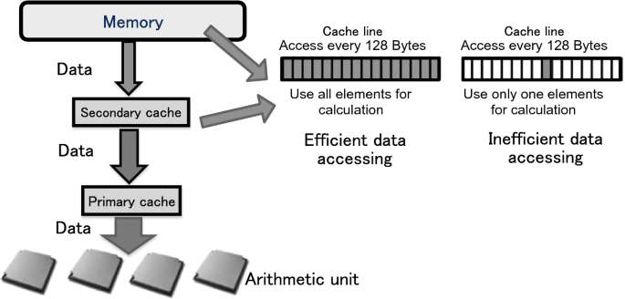

  

  Effective utilization of cache line

• (3) Effective use of the cache

  Consider the matrix–matrix product calculation of (n × n) matrices. The number of elements of the two matrices is 2n² in total and the number of computational operations is 2n³ in total for the product and the sum. If the 2n² elements are divided into multiple smaller sets of n′² and each such element set is in the cache when its computations are executed, 2n′² pieces of data are reused and 2n′³ computations can be executed. Such calculations can utilize the cache effectively and can perform high-speed calculations. In principle, for calculations that can perform n² computational operations using n data (or n³ computational calculations using n² data), high-speed calculation is possible (Fig. 2.7). As mentioned earlier, this technique is called cache blocking .

  Fig. 2.7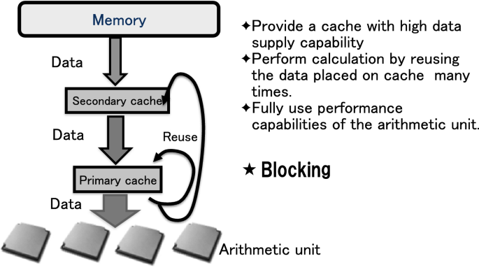

  

  Effective utilization of cache memory

  Although their capacity is much smaller than that of the L1 cache , there are registers that provide high-speed data storage locations close to the computing unit. There is thus a similar technique called register blocking in which data are blocked in the registers , but the description is omitted here.

• (4) Efficient instruction scheduling

  The K computer is equipped with 256 floating-point registers . It is important for performance improvement that the compiler schedule load, arithmetic, and store instruction belonging to different indexes of the loop index direction use these floating-point registers effectively (Fig. 2.8). If the compiler cannot find a good schedule, the performance may be improved by manually performing loop division or loop expansion.

  Fig. 2.8

  

  Efficient instruction scheduling

• (5) Effective use of SIMD arithmetic units

  The K computer CPU core has two sets of two product–sum computing units. The product–sum operation (2 operations) × two product–sum computing units × two sets allows a total of eight operations with one clock cycle. Because the operation clock of the CPU is 2 GHz, 8 operations × 2 GHz = 16 G calculation (16 GFLOPS) is the calculation peak performance per second in one core. Each of the two product–sum computing units operates as a SIMD arithmetic unit having a vector length of 2. Therefore, to realize high-performance computation, it is important that the product–sum operation works as SIMD , and that the two SIMD units operate simultaneously (Fig. 2.9).

  Fig. 2.9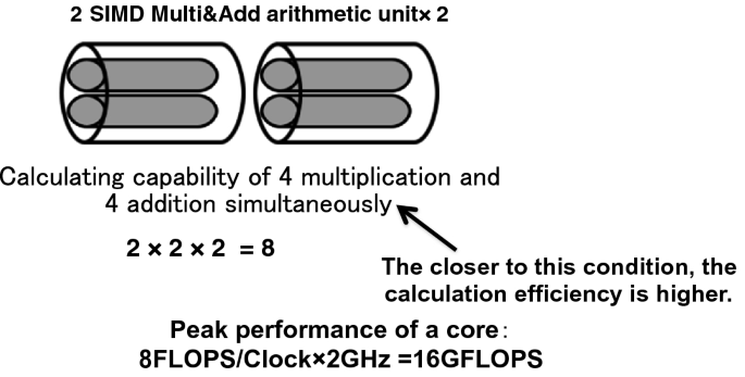

  

  Effective utilization of SIMD unit

2.8.2 Relationship Between Factors for High Performance and Required B/F Values

From the viewpoint of single-CPU performance in Sect. 1.2, we showed that applications can be classified into two types in which the required B/F value is large or small. For each of these types, we show the relationship between the type and five elements for obtaining the high performance shown in Sect. 2.8.1.

For applications with small required B/F values , high memory data transfer performance (memory bandwidth ) is not necessary in principle. It is most important to code the program to cache the data as shown in point (3) above. Next, because the L2 cache is accessed line by line, coding the program to utilize the data on each line of the L2 cache effectively (that is, point (2) above) is important (it is not necessary if the data are in the L1 cache). After realizing points (2) and (3), points (4) and (5) become important.

For applications with large required B/F values , it is important that the memory bandwidth should be utilized as fully as possible. It is more important to use the full memory bandwidth than to maximize the CPU computing performance. For these applications, the most important points are (1) and (2) above for obtaining the high performance shown in Sect. 2.8.1. It may be possible to reuse some cached data even though most data are accessed from memory, in which case point (3) becomes important. When points (1) to (3) are satisfied and the data necessary for calculation are supplied to the computing unit effectively, it is important to achieve efficient instruction scheduling in order to use these data efficiently and make effective use of the SIMD arithmetic units (points (4), (5)).

As seen here, the method required for the performance tuning varies depending on the required B/F value .

2.8.3 Thread Parallelization Common to Large and Small Required B/F Values

Regardless of whether the required B/F value is large or small, thread parallelization is indispensable for improving the single-CPU performance. Thread parallelization is impossible if there is a dependency relationship in the target loop, so the coloring method has been studied to eliminate dependencies. However, the coloring method sometimes leads to the deterioration of single-CPU performance by increasing the number of iterations. The coloring method is explained in detail in Chap. 3.

2.8.4 When the Required B/F Value Is Small: DGEMM Conversion

As in the Gram–Schmidt orthogonalization shown below, it is sometimes possible to rewrite processes that use matrix–vector products in the normal coding to use matrix–matrix products . As described in Sect. 2.6, because the required Gram–Schmidt processing of the matrix–vector product program is large, high single-CPU performance cannot be expected. However, if it can be rewritten as a matrix–matrix product , the required B/F value can be reduced, and higher single-CPU performance can be expected. By using this matrix–matrix product as the mathematical library BLAS level 3 subroutine DGEMM , it becomes possible to calculate with very high performance optimized for each computer [5].

If we code the Gram–Schmidt orthogonalization algorithm straightforwardly, it becomes an algorithm to calculate the vector $(\psi_{1}^{{\prime }} , \psi_{2}^{{\prime }} , \ldots , \psi_{i}^{{\prime }} , \ldots$) as the orthogonalization of the vector $(\psi_{1} , \psi_{2} , \ldots , \psi_{i}^{{\prime }} , \ldots$), as shown in Fig. 2.10. This algorithm is coded with the matrix–vector product of the matrix $\left\langle {\psi_{i}^{{\prime }} |\psi_{j} } \right\rangle$ and vector $\left| {\psi_{i}^{{\prime }} } \right\rangle$. The indices 1, 2, …, i are parallelized for each process.

Fig. 2.10

Original processing of Gram–Schmidt orthogonalization

Consider dividing this algorithm into a triangular part and a rectangular part, as shown in Fig. 2.11. Each rectangular part in the direction $(\psi_{1} , \psi_{2} , \ldots ,\psi^{\prime}_{i} , \ldots$) is parallelized for each process. First, in the process responsible for the triangular part, we use the original matrix–vector product algorithm. In the example in Fig. 2.11, the calculation of triangles for calculating ψ₁ and ψ₂ corresponds to this explanation. Using the calculated (ψ₁, ψ₂) data and calculating the square part in each process, this calculation can use the matrix–matrix product . In the example in Fig. 2.11, the calculation of the square in the left column using ψ₁ and ψ₂ corresponds to this explanation. The second triangular part is calculated using the original matrix–vector product algorithm. Similarly, ψ₃ and ψ₄ can be calculated perfectly in the example of Fig. 2.11. By repeating this process, it becomes possible to calculate the Gram–Schmidt orthogonalization using the matrix–matrix product . In the actual algorithm, the triangular part is recursively divided into a rectangular part and a triangular part as shown in Fig. 2.11, so that the matrix–matrix product calculation can be used as much as possible.

Fig. 2.11

Matrix–matrix productization of Gram–Schmidt orthogonalization

2.8.5 When the Required B/F Value Is Small: Cache Blocking

As described in Sect. 2.6, high single-CPU performance can be obtained by performing cache blocking , as in the matrix–matrix multiplication. The Coulomb force calculation in classical MD is one example. In this calculation, however, discontinuous list access is required to specify the particle pair, which degrades the single-CPU performance. Changing the blocking by rearranging the discontinuous data using the following procedure improves the single-CPU performance. This procedure is illustrated in Fig. 2.12.

Fig. 2.12

Cache blockzation

• (1) Copy the N discontinuous data to a continuous area to enable blocking in the cache.

• (2) Perform the calculation N² times using N pieces of data.

• (3) Copy and return continuous calculated results to the discontinuous area.

In general, the copies of (1) and (3) require order-N processing, so the processing time is smaller than the computation time of order N². Therefore, even if the copy is troublesome, a reduction in total execution time may be obtained.

2.8.6 When the Required B/F Value Is Small and the Loop Body Is Complex

When the loop body of a code is complex, the compiler may not be able to correctly interpret the required processing. In this case, more arrays are used in the loop, so more registers corresponding to the arrays are required, and there is a tendency for register shortage to occur. For these reasons, this type of application often fails to provide adequate performance even when the data are in the cache . There is no general solution for this problem, and we can only rewrite the code to achieve loop division, array index replacement, or array integration individually for each application.

2.8.7 Optimizing the Single-CPU Performance: When the Required B/F Value Is Large

The procedure for improving the single-CPU performance is shown in Fig. 2.13.

Fig. 2.13

Steps for improving performance

• (1) Profiler measurements

  Modern supercomputers are equipped with a profiler for acquiring performance information. The K computer has an excellent profiler function that can acquire abundant and useful information relating to the memory, cache , and arithmetic unit. This profiler should be used to measure the performance of the application kernel.

• (2) Detection of problems using the profiler’s measurement results

  Analyze the problem by looking at the profiler measurements. As described in Sect. 2.8.2, in applications that cannot efficiently utilize the caches , the important point for achieving high single-CPU performance is to use the memory performance fully. The profiler information includes the memory bandwidth used, and we can analyze the cause of the problem if the memory performance is poor.

• (3) Performance estimation

  Estimate the performance of the kernel using the performance estimation model (see Sect. 2.8.8). If the actual measurement results do not reach the estimation results, extend the analysis of step (2). Performance estimation is very important to judge the extent of tuning work required and where to stop.

• (4) Performance tuning

  We consider the available performance improvement methods and perform tuning work based on the results of the analysis of step (2). Work continues until the estimated performance is achieved.

• (5) Predict the performance of the improved version

  Consider further methods of performance improvement and perform more tuning work. The performance of the kernel after further tuning is estimated according to the roof-line model (see Sect. 2.8.8).

• (6) Further performance tuning

  Measure performance and analyze the results for the revised code after tuning. This cycle is repeated until the estimated result is approached.

2.8.8 Performance Estimation: When the Required B/F Value Is Large

Here, the performance estimation method when the required B/F value is large is described. The roof-line performance prediction model is used when data access is limited to the memory accesses and data access from the cache memory is not considered [6].

We define the theoretical memory bandwidth of the hardware as B, and the theoretical peak performance is defined as F. If the operational intensity of the application using the required FLOP value f of the application and the required byte value b of the application is X = f/b, the effective performance of the application is represented by min {F, BX}. The operational intensity is the reciprocal of the B/F value . In this performance estimation model, an application that has the same operational intensity as the hardware can achieve peak performance . If the predicted performance of the application requires an operational intensity smaller than the operational intensity of the hardware, the model is proportional to the operational intensity required by the application. What we have described here is shown in Fig. 2.14. The performance of a memory-intensive application with a high required B/F value can be estimated more accurately by replacing the theoretical memory bandwidth of this model with the effective memory bandwidth [7].

Fig. 2.14

Roofline model

2.8.9 Performance Optimization of the Sparse Matrix–Vector Product: When the Required B/F Value Is Large

A typical application with high required B/F value is the sparse matrix–vector product . This calculation often appears when discretizing partial differential equations. The features of the sparse matrix–vector product are shown below.

In general, when solving physical three-dimensional problems, the coefficients are three-dimensional and occupy sparse matrices to form three-dimensional arrays. However, these arrays may be expressed as one-dimensional or two-dimensional arrays for coding. In either case, the required memory capacity is large, so it is common to consume the memory bandwidth . However, the coefficient matrices may also be expressed not in three dimensions but in one- or two-dimensional arrays, or the coefficients may be represented as scalar quantities. In these cases, the calculation of the product of a sparse matrix and a vector does not consume as much memory bandwidth and the arrays can be stored in caches or registers . While the vectors are generally three-dimensional arrays when solving three-dimensional problems physically, they may, like the sparse matrices, be expressed as one- or two-dimensional arrays to simplify coding. An important feature of the vector arrays is that there is M or around M reusability when the average number of elements included in each row of the matrix is M and the dimension of the vector is L. Because the number of operations for the sparse matrix–vector products is M × L for each addition and multiplication, and the number of elements of vectors being used for performing operations is L, one element of the vector is referred to on average M times. Therefore, the memory bandwidth capacity of the vector is about 1/M of the memory bandwidth capacity of the matrix. Although access to the vectors also consumes memory bandwidth , the efficient utilization of the cache using the M reusability shown here is important for improving single-CPU performance.

2.8.10 Performance Optimization of the Sparse Matrix–Vector Product: Required B/F Value Is Large and List Vectors Used

For the sparse matrix–vector product discussed in Sect. 2.8.9, a stencil calculation in which the vector is continuously accessed is assumed. In addition to having the high required B/F value , there are applications for which the vectors are accessed using a list. In this case as well, because the vectors are reusable, it is important to make effective use of the cache . However, because the vector is not continuously accessed, it is difficult to use cache memory effectively. For such applications, the cache can be utilized more efficiently by rearranging the order of the discrete points according to their physical positions, as discussed in the section on FFB in Chap. 3.

Exercises

• 1. Show that numerical solutions of differential equations by discretization are obtained using simultaneous linear equations, where A is a square matrix and x and b are vectors:

  $$ {\text{Ax}} = {\text{b}}. $$

  (2.1)

• 2. Show that the simultaneous linear Eq. (2.1) can be transformed to:

  $$ {\text{x}} = {\text{Bx}} + {\text{b}}, $$

  (2.2)

  where B is a square matrix. When considering x⁰, x¹, x², that satisfy Eq. (2.3), if the column of vectors converges to vector x, show that the vector x satisfies Eq. (2.1):

  $$ x^{{\left( {m + 1} \right)}} = Bx^{\left( m \right)} + b $$

  (2.3)

• 3. The method of solving Eq. (2.2) as Eq. (2.3) is called an iterative method. One such method is the Jacobi method. If the equation to be solved is (2.1), the formula for the Jacobi iterative method is expressed as (2.4) and (2.5).

  $$ {\text{x}}^{{\left( {m + 1} \right)}} = D^{ - 1} \left( {E + F} \right){\text{x}}^{{\left( {m + 1} \right)}} + D^{ - 1} b $$

  (2.4)
  $$ \begin{aligned} a_{ii} x_{i}^{{\left( {m + 1} \right)}} & = - \sum a_{ij}^{\left( m \right)} + b_{j} \\ x_{i}^{{\left( {m + 1} \right)}} & = - \mathop \sum \limits_{j = 1,j \ne i}^{n} \left( {\frac{{a_{ij} }}{{a_{ii} }}} \right)x_{ij}^{\left( m \right)} + \frac{b}{{a_{ii} }}, \\ \end{aligned} $$

  (2.5)

  where D, E, and F contain the diagonal elements of A, the lower triangular matrix of A, and the upper triangular matrix of A, respectively. Derive (2.4) and (2.5), which are expressions of the Jacobi method.

• 4. Code the Jacobi method in an appropriate programming language and parallelize it with MPI and/or OpenMP and investigate the parallelization efficiency . (The code for the nonparallel version of the Jacobi method can be found in textbooks or on several websites.)

References

M. Terai, E. Tomiyama, H. Murai, K. Minami, M. Yokokawa, in Third International Workshop on Parallel Software Tools and Tool Infrastructures (PSTI2012), vol. 434 (2012)
M. Terai, E. Tomiyama, H. Murai, K. Kumahata, S. Hamada, S. Inoue, A. Kuroda, Y. Hasegawa, K. Minami, M. Yokokawa, in Proceedings of High Performance Computing and Computational Science (in Japanese), vol. 84 (2013)
K. Asanović, R. Bodik, B.C. Catanzaro, J.J. Gebis, P. Husbands, K. Keutzer, D.A. Patterson, W.L. Plishker, J. Shalf, S.W. Williams, K.A. Yelick, Tech. Rep. of UCB/EECS-2006-183 (2006)
T. Yokozawa, D. Takahashi, T. Boku, M. Sato, in Proceedings of Fourth International Workshop on Parallel Matrix Algorithms and Applications (PMAA’06), vol. 37 (2006)
S. Williams, A. Waterman, D. Patterson, Commun. ACM 52, 65 (2009)
K. Minami, S. Inoue, S. Shigenobu, T. Maeda, Y. Hasegawa, A. Kuroda, M. Terai, M. Yokokawa, in Proceedings of High Performance Computing and Computational Science (in Japanese), vol. 23 (2012)
Author information
Authors and Affiliations
Corresponding author
Editor information
Editors and Affiliations
Rights and permissions
Copyright information
© 2019 Springer Nature Singapore Pte Ltd.
About this chapter
Cite this chapter
Minami, K. (2019). Performance Optimization of Applications. In: Geshi, M. (eds) The Art of High Performance Computing for Computational Science, Vol. 2. Springer, Singapore. https://doi.org/10.1007/978-981-13-9802-5_2
Download citation
DOI: https://doi.org/10.1007/978-981-13-9802-5_2
Published:
Publisher Name: Springer, Singapore
Print ISBN: 978-981-13-9801-8
Online ISBN: 978-981-13-9802-5
eBook Packages: Computer ScienceComputer Science (R0)