Models and Algorithms for Least Square Interval-Valued Nucleoli of Cooperative Games with Interval-Valued Payoffs

Abstract

The aim of this paper is to develop a new method for computing least square interval-valued nucleoli of cooperative games with interval-valued payoffs, which usually are called interval-valued cooperative games for short. In this methodology, based on the square excess which can be intuitionally interpreted as a measure of the dissatisfaction of the coalitions, we construct a quadratic programming model for least square interval-valued prenucleolus of any interval-valued cooperative game and obtain its analytical solution, which is used to determine players’ interval-valued imputations via the designed algorithms that ensure the nucleoli always satisfy the individual rationality of players. Hereby the least square interval-valued nucleoli of interval-valued cooperative games are determined in the sense of minimizing the difference of the square excesses of the coalitions. Moreover, we discuss some useful and important properties of the least square interval-valued nucleolus such as its existence and uniqueness, efficiency, individual rationality, additivity, symmetry, and anonymity.

1 Introduction

Due to uncertainty and imprecision in real economic management situations, player coalitions’ values usually have to be estimated. Recently, intervals seem to be suitable for employing to deal with inherited imprecision or vagueness in coalitions’ values and hereby there appears an important type of cooperative games with interval-valued data, which often are called interval-valued cooperative games for short [1, 2]. A good example may be the interval bankruptcy games with interval claims [3]. Specifically, Branzei et al. [3] introduced interval-valued cooperative games which are used to handle bankruptcy situations where the estate is known with certainty while claims belong to known bounded intervals of real numbers and hereby defined two Shapley-like values for solving the interval-valued cooperative games. Obviously, interval-valued cooperative games are remarkably different from classical cooperative games from the point of view of the data type of the player coalitions’ values. The coalitions’ values of interval-valued cooperative games are expressed with intervals but that of classical cooperative games are expressed with real numbers [4, 5].

Lately, interval-valued cooperative games have attracted attention of researchers and their solution concepts have applied to many fields such as business [6], operations research [7], economy, modern finance, climate negotiations and policy, tourism management [2], environmental management, and pollution control. To be more precise, Branzei et al. [3] firstly defined two Shapley-like values, which associate vectors of intervals with interval-valued cooperative games of the interval bankruptcy problems with interval claims, and studied the interrelations among using the arithmetic of intervals [8]. To place the models of interval-valued cooperative games within the cooperative game theory and to motivate continued interest in theory and application development, Branzei et al. [1] gave a good survey that discussed how the models of interval-valued cooperative games extended the cooperative game theory, and reviewed their existing and potential applications in economic management and business situations with interval data. Alparslan Gök et al. [4] studied the properties of the interval-valued Shapley value on the class of size monotonic interval-valued cooperative games and gave an axiomatic characterization of the interval-valued Shapley value on a special subclass of interval-valued cooperative games. Kimms and Drechsel [6] proposed a general mathematical programming algorithm which can be used to find an element in the interval-valued core. Hong and Li [9] constructed an auxiliary nonlinear programming model and hereby proposed a corresponding effective bisection method for computing elements of interval-valued cores of interval-valued n-person cooperative games by introducing the satisfaction degree index (or fuzzy ranking index) of interval comparison. Theoretically, Branzei et al. [10] defined the interval-valued cores of interval-valued cooperative games through discussing the interval-valued square dominance and interval-valued dominance imputations. Alparslan Gök et al. [11] introduced some set-valued solution concepts of interval-valued cooperative games, which include the interval-valued core, the interval-valued dominance core, and the interval-valued stable sets. Alparslan Gök et al. [12] extended the classical two-person cooperative game theory to two-person cooperative games with interval data and studied the interval-valued core, balancedness, superadditivity, and some other properties.

However, it is easy to find that most of the aforementioned works used the Moore’s interval operations [8], especially the Moore’s interval subtraction, which usually enlarges uncertainty of the resulted interval. This case usually is not accordant with real economic management situations. Therefore, the aim of this paper is to develop simple and effective quadratic programming methods for solving interval-valued cooperative games. More precisely, based on the differences of the square excesses of the player coalitions, we construct two quadratic programming models and obtain their analytical solutions, i.e., least square interval-valued prenucleoli and nucleoli, which are used to determine players’ interval-valued imputations through using the designed algorithms which ensure that they satisfy the individual rationality of players. Hereby, the least square interval-valued prenucleoli and nucleoli of interval-valued cooperative games are determined in the sense of minimizing the difference of the square excesses of the player coalitions. The quadratic programming methods proposed in this paper are remarkably different from the aforementioned methods. On the one hand, the developed methods can provide analytical formulae for determining the least square interval-valued prenucleoli and nucleoli of interval-valued cooperative games and hereby obtain the interval-valued imputations of players. On the other hand, the developed methods can effectively avoid the Moore’s interval subtraction [8].

The rest of this paper is arranged as follows. In the next section, we briefly review the interval-valued cooperative games and their solution concepts and hereby define the square excesses of players’ coalitions on interval-valued payoff vector to measure the dissatisfaction of the coalitions. In Sect. 3, we construct two quadratic programming models based on the square excesses of the player coalitions to compute the least square interval-valued prenucleoli and nucleoli of interval-valued cooperative games. The effective algorithm is designed to determine players’ interval-valued imputations through considering the individual rationality of players. Furthermore, we discuss some important and useful properties of the least square interval-valued prenucleoli and nucleoli of interval-valued cooperative games. The quadratic programming models and algorithms are illustrated with a numerical example about the optimal allocation of the cooperative profits of joint production and the computational result is analyzed in Sect. 4. The validity, applicability, and advantages of the methods proposed in this paper are shown and some remarks on further research are discussed in the last section.

2 Notations of Intervals and Interval-Valued Cooperative Games

2.1 Interval Notations and Arithmetic Operations

To facilitate introducing interval-valued cooperative games, we firstly review the concepts of intervals and their distances as well as interval arithmetic operations.

Usually, $\bar{a} = [a_{L} ,a_{R} ] = \{ a\left| {a \in {\text{R}},a_{L} \le a \le a_{R} } \right.\}$ is used to express an interval, where ${\text{R}}$ is the set of real numbers, $a_{L} \in {\text{R}}$ and $a_{R} \in {\text{R}}$ are called the lower bound and the upper bound of the interval $\bar{a}$, respectively. Let $\bar{R}$ be the set of intervals on the set ${\text{R}}$.

Clearly, if $a_{L} = a_{R}$, then the interval $\bar{a} = [a_{L} ,a_{R} ]$ degenerates to a real number, denoted by $a$, where $a = a_{L} = a_{R}$. Conversely, a real number $a$ may be written as an interval $\bar{a} = [a,a]$. Therefore, intervals are a generalization of real numbers. That is to say, real numbers are a special case of intervals [2, 8].

If $a_{L} \ge 0$, then $\bar{a} = [a_{L} ,a_{R} ]$ is called a non-negative interval, denoted by $\bar{a} \ge 0$. Likewise, if $a_{R} \le 0$, then $\bar{a}$ is called a non-positive interval, denoted by $\bar{a} \le 0$. If $a_{L} > 0$, then $\bar{a}$ is called a positive interval, denoted by $\bar{a} > 0$. If $a_{R} < 0$, then $\bar{a}$ is called a negative interval, denoted by $\bar{a} < 0$.

To facilitate the sequent discussion, we briefly review arithmetic operations of intervals such as the equality, the addition, and the scalar multiplication [2, 8, 13].

Assume that $\bar{a} = [a_{L} ,a_{R} ]$ and $\bar{b} = [b_{L} ,b_{R} ]$ be two intervals on the set $\bar{R}$. Then, $\bar{a}$ is equal to $\bar{b}$ if and only if $a_{L} = b_{L}$ and $a_{R} = b_{R}$, denoted by $\bar{a} = \bar{b}$.

$$ \bar{a} + \bar{b} = [a_{L} + b_{L} ,a_{R} + b_{R} ]. $$

(1)

The scalar multiplication of a real number $\gamma \in R$ and an interval $\bar{a}$ is defined as follows:

$$ \gamma \bar{a} = \left\{ {\begin{array}{*{20}c} {[\gamma a_{L} ,\gamma a_{R} ]} & { (\gamma \ge 0 )} \\ {[\gamma a_{R} ,\gamma a_{L} ]} & { (\gamma < 0 )} \\ \end{array} } \right. $$

(2)

Clearly, the above arithmetic operations of intervals are a generalization of those of real numbers.

In most management situations, we usually have to compare or rank intervals. However, ranking intervals or interval comparison is a difficult and an important problem. In a parallel way to comparison of the real numbers, Moore [8] firstly proposed the order relation between intervals as follows:

$$ \bar{a} \le \bar{b}\,\,{\text{if}}\,{\text{and}}\,{\text{only}}\,{\text{if}}\,a_{L} \le b_{L} \,{\text{and}}\,a_{\text{R}} \le b_{R} , $$

(3)

which is simply called the Moore’s order relation between intervals.

To measure differences between intervals, we give the distance concept as follows.

Definition 1.

Assume that $\bar{a}$ and $\bar{b}$ be two intervals on the set $\bar{R}$. If a mapping $d:\bar{R} \times \bar{R} \mapsto {\text{R}}$ satisfies the three properties (1)–(3) as follows:

• (1) Non-negativity: $d(\bar{a},\bar{b}) \ge 0$;

• (2) Symmetry: $d(\bar{a},\bar{b}) = d(\bar{b},\bar{a})$;

• (3) Trigonometrical inequality relation: $d(\bar{a},\bar{b}) \le d(\bar{a},\bar{c}) + d(\bar{c},\bar{b})$ for any interval $\bar{c}$ on the set $\bar{R}$, then $d(\bar{a},\bar{b})$ is called the distance between the intervals $\bar{a}$ and $\bar{b}$.

It is easy to see from Definition 1 that the distance between intervals is a natural generalization of that of the set of real numbers.

Obviously, there are various forms of distances between intervals which satisfy Definition 1. For instance, to meet the need of modeling interval-valued cooperative games in the subsequent sections, we define the distance between two intervals $\bar{a} \in \bar{R}$ and $\bar{b} \in \bar{R}$ as follows:

$$ D(\bar{a},\bar{b}) = (a_{L} - b_{L} )^{2} + (a_{R} - b_{R} )^{2} . $$

(4)

It is easy to see that Eq. (4) is very similar to the distance between two points in the two-dimension Euclidean space.

Theorem 1.

$D(\bar{a},\bar{b})$ defined by Eq. (4) is the distance between the intervals $\bar{a} \in \bar{R}$ and $\bar{b} \in \bar{R}$.

Proof.

We need to validate that $D(\bar{a},\bar{b})$ defined by Eq. (4) satisfies the three properties (1)–(3) of Definition 1, respectively.

It is easy to see from Eq. (4) that $D(\bar{a},\bar{b}) \ge 0$ and $D(\bar{a},\bar{b}) = D(\bar{b},\bar{a})$ for any intervals $\bar{a}$ and $\bar{b}$. Namely, $D(\bar{a},\bar{b})$ satisfies the properties (1) and (2) of Definition 1.

For any interval $\bar{c}$ on the set $\bar{R}$, where $\bar{c} = [c_{L} ,c_{R} ]$, it is easily derived from Eq. (4) that

$$ \begin{aligned} D(\bar{a},\bar{b}) = & (a_{L} - b_{L} )^{2} + (a_{R} - b_{R} )^{2} \\ \, \le & [(a_{L} - c_{L} )^{2} + (c_{L} - b_{L} )^{2} ] + [(a_{R} - c_{R} )^{2} + (c_{R} - b_{R} )^{2} ] \\ { = } & [(a_{L} - c_{L} )^{2} + (a_{R} - c_{R} )^{2} ] + [(c_{L} - b_{L} )^{2} + (c_{R} - b_{R} )^{2} ] \\ { = } & D(\bar{a},\bar{c}) + D(\bar{c},\bar{b}), \\ \end{aligned} $$

i.e.,

$$ D(\bar{a},\bar{b}) \le D(\bar{a},\bar{c}) + D(\bar{c},\bar{b}). $$

Therefore, $D(\bar{a},\bar{b})$ satisfies the property (3) of Definition 1. Thus, we have proven that $D(\bar{a},\bar{b})$ defined by Eq. (4) is the distance between the intervals $\bar{a}$ and $\bar{b}$.

It is noted that the square appears in Eq. (4). In fact, Eq. (4) is the square of the distance between the intervals. In the sequent, the distance between two intervals is referred to the square of the distance given by Eq. (4) unless otherwise specified.

2.2 Interval-Valued Cooperative Games and Notations

A $n$-person interval-valued cooperative game in characteristic function form is an ordered-pair ${<}N,\bar \upsilon{>}$, where $N = \{ 1,2, \cdots ,n\}$ is the set of $n$ players, each subset $S\, \subseteq \,N$ is called a coalition of the player set $N$, and $\bar{\upsilon }:2^{N} \to {\mathbb{R}}$ is the interval-valued characteristic function of players’ coalitions. $2^{N}$ denotes the set of coalitions of the player set $N$. Obviously, $N$ is the grand coalition. For each coalition $S\, \subseteq \,N$, its size is denoted by $s$, which represents the number of players in the coalition $S$. The interval $\bar{\upsilon }(S) = [\upsilon_{L} (S),\upsilon_{R} (S)]$ represents the range of reward (or profit) that the coalition $S$ can achieve on its own if all the players in it act together, where the lower bound $\upsilon_{L} (S)$ of the interval $\bar{\upsilon }(S)$ is the minimal reward of the coalition $S$ and the upper bound $\upsilon_{R} (S)$ of the interval $\bar{\upsilon }(S)$ is the maximal reward of the coalition $S$. The interpretation of interval-valued cooperative games is that a coalition $S\, \subseteq \,N$ can obtain for its members a worth that is somewhere in the interval $\bar{\upsilon }(S)$. Stated as the above Sect. 2.1, we stipulate $\bar{\upsilon }(\varnothing ) = [0,0]$, where $\varnothing$ is an empty set. Note that usually $\bar{\upsilon }(\varnothing )$ can be simply written as $\bar{\upsilon }(\varnothing ) = 0$ according to the notation of intervals in Sect. 2.1. For convenience, $\bar{\upsilon }(S \cup \{ i\} )$, $\bar{\upsilon }(S\backslash \{ i\} )$, $\bar{\upsilon }(\{ i,j\} )$, and $\bar{\upsilon }(\{ i\} )$ are usually written as $\bar{\upsilon }(S \cup i)$, $\bar{\upsilon }(S\backslash i)$, $\bar{\upsilon }(i,j)$, and $\bar{\upsilon }(i)$, respectively. In the sequent, a $n$-person interval-valued cooperative game ${<}N,\bar{\upsilon}{>}$ is simply called the interval-valued cooperative game $\bar{\upsilon }$. The set of $n$-person interval-valued cooperative games $\bar{\upsilon }$ is denoted by $\bar{G}^{n}$.

3 Quadratic Programming Model for Least Square Interval-Valued Prenucleoli of Interval-Valued Cooperative Games

For any interval-valued cooperative game $\bar{\upsilon } \in \bar{G}^{n}$, it is obvious that each player’s payoff obtained from cooperation should be also an interval due to the fact that the payoff (or characteristic value) of each coalition $S\, \subseteq \,N$ is an interval. Thus, let $\bar{x}_{i} = [x_{Li} ,x_{Ri} ]$ be the interval-valued payoff which is allocated to the player $i \in N$ when the grand coalition $N$ is reached. Denote $\bar{\varvec{x}} = (\bar{x}_{1} ,\bar{x}_{2} , \cdots ,\bar{x}_{n} )^{\text{T}}$, which is the interval-valued payoff vector of $n$ players in the grand coalition $N$. For any coalition $S\, \subseteq \,N$, denote $\bar{x}(S) = \sum\limits_{i \in S} {\bar{x}_{i} }$, which represents the collective (or aggregated) interval-valued payoff of all the players in the coalition $S$. According to Eq. (1), $\bar{x}(S) = [x_{L} (S),x_{R} (S)]$ can be expressed as the following interval:

$$ \bar{x}(S) = [\sum\limits_{i \in S} {x_{Li} } ,\sum\limits_{i \in S} {x_{Ri} } ]. $$

In a similar way to the definitions of the efficiency and individual rationality of the classical cooperative game [2, 14], if an interval-valued payoff vector $\bar{\varvec{x}}$ satisfies both the efficiency and individual rationality conditions as follows:

$$ \sum\limits_{i = 1}^{n} {\bar{x}_{i} } = \bar{\upsilon }(N) $$

(5)

and

$$ \bar{x}_{i} \ge \bar{\upsilon }(i)\;(i = 1,2, \cdots ,n), $$

(6)

respectively, then $\bar{\varvec{x}}$ is called an imputation of the interval-valued cooperative game $\bar{\upsilon } \in \bar{G}^{n}$. In other word, an interval-valued payoff vector $\bar{\varvec{x}}$ is said to be efficient or a preimputation if the efficiency condition $\bar{x}(N) = \bar{\upsilon }(N)$ is valid. Further, $\bar{\varvec{x}}$ is said to be an imputation if the individual rationality conditions $\bar{x}_{i} \ge \bar{\upsilon }(i)$ for all players $i \in N$ are also satisfied. $\bar{I}^{\Pr } (\bar{\upsilon })$ and $\bar{I}(\bar{\upsilon })$ denote the sets of interval-valued preimputations and imputations of the interval-valued cooperative game $\bar{\upsilon } \in \bar{G}^{n}$, respectively.

Using Eqs. (1) and (3), Eqs. (5) and (6) can be rewritten as follows:

$$ \left\{ \begin{aligned} \sum\limits_{i = 1}^{n} {x_{Li} } = \upsilon_{L} (N) \hfill \\ \sum\limits_{i = 1}^{n} {x_{Ri} } = \upsilon_{R} (N) \hfill \\ \end{aligned} \right. $$

(7)

and

$$ \left\{ {\begin{array}{*{20}l} {x_{Li} \ge \upsilon_{L} (i)\; (i = 1,2, \cdots ,n)} \hfill \\ {x_{Ri} \ge \upsilon_{R} (i)\; (i = 1,2, \cdots ,n),} \hfill \\ \end{array} } \right. $$

(8)

respectively.

For any interval-valued payoff vector $\bar{\varvec{x}}$ and any coalition $S\, \subseteq \,N$, where $S \ne \varnothing$, according to Eq. (4), denote

$$ e(S,\bar{x}) = (\upsilon_{L} (S) - x_{L} (S))^{2} + (\upsilon_{R} (S) - x_{R} (S))^{2} , $$

(9)

which is just the square of the distance between the intervals $\bar{x}(S)$ and $\bar{\upsilon }(S)$. Then, $e(S,\bar{x})$ is called the square excess of the coalition $S$ on the interval-valued payoff vector $\bar{\varvec{x}}$.

Usually, for any coalition $S\, \subseteq \,N$, we use $e_{L} (S,\bar{x})$ to express $\upsilon_{L} (S) - x_{L} (S)$, i.e.,

$$ e_{L} (S,\bar{x}) = \upsilon_{L} (S) - x_{L} (S), $$

(10)

which is called the lower bound of the excess of the coalition $S$ on the interval-valued payoff vector $\bar{\varvec{x}}$. Likewise, we use $e_{R} (S,\bar{x})$ to represent $\upsilon_{R} (S) - x_{R} (S)$, i.e.,

$$ e_{R} (S,\bar{x}) = \upsilon_{R} (S) - x_{R} (S), $$

(11)

which is called the upper bound of the excess of the coalition $S$ on $\bar{\varvec{x}}$. Therefore, $e(S,\bar{x})$ can be rewritten as follows:

$$ e(S,\bar{x}) = (e_{L} (S,\bar{x}))^{2} + (e_{R} (S,\bar{x}))^{2} . $$

It is noted that $e(S,\bar{x})$ can be interpreted as a measure of the dissatisfaction of the coalition $S$ if $\bar{\varvec{x}}$ were suggested as a final interval-valued payoff vector for all the players in the grand coalition. Obviously, $e(S,\bar{x}) \ge 0$. Further, the square excess $e(N,\bar{x})$ of the grand coalition $N$ on $\bar{x}$ is equal to 0 if the interval-valued payoff vector $\bar{\varvec{x}}$ satisfies the efficiency. Hence, the greater $e(S,\bar{x})$ the more unfair the coalition $S$.

Least square interval-valued prenucleoli and nucleoli are an important type of solutions for interval-valued cooperative games. In a paralleled way to the definitions of the prenucleoli and nucleoli [15, 16] of classical cooperative games, we can define the least square interval-valued prenucleoli and nucleoli of interval-valued cooperative games based on the square excesses of coalitions on the interval-valued payoff vectors.

The least square interval-valued prenucleolus of an interval-valued cooperative game would choose an interval-valued payoff vector to minimize the sum of the square excesses from the preimputation set according to the lexicographical order. Whereas, the least square interval-valued nucleolus would choose an interval-valued payoff vector to minimize the sum of the square excesses from the imputation set. In both cases, the key problem to obtain least square interval-valued prenucleoli and nucleoli of interval-valued cooperative games is to minimize the maximal complaint with the square excess of a coalition on an interval-valued payoff vector. This selection is regarded as equitable and reasonable. To attain the minimum of $\sum\limits_{S \subseteq N} {e(S,\bar{x})}$ and balance the gain of each player $i \in N$, we will choose the interval-valued payoff vector to minimize the sum of the squares of the differences between the excesses of the coalitions and their means (or average excesses). Namely, we try to find the interval-valued payoff vector so that the resulting excesses are the closest to the means under the least square criterion. Thus, combining with Eq. (7), solving a least square interval-valued prenucleolus of any interval-valued cooperative game can be transformed into solving the constructed quadratic programming model as follows:

$$ \begin{aligned} & \hbox{min} \left\{ {\sum\limits_{S \subseteq N,S \ne \varnothing } {[(e_{L} (S,\bar{x}) - e_{Lm} (S,\bar{x})} )^{2} + (e_{R} (S,\bar{x}) - e_{Rm} (S,\bar{x}))^{2} ]} \right\} \\ & {\text{s}} . {\text{t}} .\left\{ {\begin{array}{*{20}l} {\sum\limits_{i = 1}^{n} {x_{Li} } = \upsilon_{L} (N)} \hfill \\ {\sum\limits_{i = 1}^{n} {x_{Ri} } = \upsilon_{R} (N),} \hfill \\ \end{array} } \right. \\ \end{aligned} $$

(12)

where the summation is taken over all nonempty coalitions $S\, \subseteq \,N$, and $e_{Lm} (S,\bar{x})$ and $e_{Rm} (S,\bar{x})$ are the means of the excesses of coalitions on $\bar{\varvec{x}}$, i.e.,

$$ e_{Lm} (S,\bar{x}) = \frac{1}{{2^{n - 1} }}\sum\limits_{S \subseteq N,S \ne \varnothing } {e_{L} (S,\bar{x})} $$

(13)

and

$$ e_{Rm} (S,\bar{x}) = \frac{1}{{2^{n - 1} }}\sum\limits_{S \subseteq N,S \ne \varnothing } {e_{R} (S,\bar{x})} . $$

(14)

Analogously, combining with Eqs. (7) and (8), solving a least square interval-valued nucleolus of any interval-valued cooperative game can be converted into solving the constructed quadratic programming model as follows:

$$ \begin{aligned} \\ & \hbox{min} \{ \sum\limits_{S \subseteq N,S \ne \varnothing } {[(e_{L} (S,\bar{x}) - e_{Lm} (S,\bar{x})} )^{2} + (e_{R} (S,\bar{x}) - e_{Rm} (S,\bar{x}))^{2} ]\} \\ & {\text{s}} . {\text{t}} .\left\{ {\begin{array}{*{20}l} {\sum\limits_{i = 1}^{n} {x_{Li} } = \upsilon_{L} (N)} \hfill \\ {\sum\limits_{i = 1}^{n} {x_{Ri} } = \upsilon_{R} (N)} \hfill \\ {x_{Li} \ge \upsilon_{L} (i) \, \;{ (}i = 1,2, \cdots ,n)} \hfill \\ {x_{Ri} \ge \upsilon_{R} (i)\;{ (}i = 1,2, \cdots ,n).} \hfill \\ \end{array} } \right. \\ \end{aligned} $$

(15)

It is easily observed the following conclusion: for any interval-valued cooperative game $\bar{\upsilon } \in \bar{G}^{n}$, if an interval-valued payoff vector $\bar{\varvec{x}}$ satisfies the efficiency, then the sum of the lower (or upper) bounds of the excesses of all coalitions $S\, \subseteq \,N$ on $\bar{\varvec{x}}$ is the same as that on any other interval-valued payoff vector which also satisfies the efficiency. In fact, due to the assumption that $\bar{\varvec{x}}$ is an interval-valued payoff vector which satisfies the efficiency, then we have

$$ \begin{aligned} \sum\limits_{S \subseteq N,S \ne \varnothing } {e_{L} (S,\bar{x})} & = \sum\limits_{S \subseteq N,S \ne \varnothing } {(\upsilon_{L} (S) - x_{L} (S))} \\ \, & \, = \sum\limits_{S \subseteq N,S \ne \varnothing } {\upsilon_{L} (S) - } \sum\limits_{S \subseteq N,S \ne \varnothing } {x_{L} (S)} \\ \, & \, = \sum\limits_{S \subseteq N,S \ne \varnothing } {\upsilon_{L} (S) - } \frac{1}{2}[\sum\limits_{S \subseteq N,S \ne \varnothing } {x_{L} (S)} + \sum\limits_{S \subseteq N,S \ne \varnothing } {x_{L} (N\backslash S)} + x_{L} (N)] \\ \, & = \sum\limits_{S \subseteq N,S \ne \varnothing } {\upsilon_{L} (S) - } \frac{1}{2}\sum\limits_{S \subseteq N,S \ne \varnothing } {(x_{L} (S) + x_{L} (N\backslash S))} - \frac{1}{2}x_{L} (N) \\ \, & \, = \sum\limits_{S \subseteq N,S \ne \varnothing } {\upsilon_{L} (S) - } \frac{1}{2}(2^{n} - 1)x_{L} (N) - \frac{1}{2}x_{L} (N) \\ \, & \, = \sum\limits_{S \subseteq N,S \ne \varnothing } {\upsilon_{L} (S) - } 2^{n - 1} x_{L} (N) \\ \, & \, = \sum\limits_{S \subseteq N,S \ne \varnothing } {\upsilon_{L} (S) - } 2^{n - 1} \upsilon_{L} (N), \\ \end{aligned} $$

i.e.,

$$ \sum\limits_{S \subseteq N,S \ne \varnothing } {e_{L} (S,\bar{x})} = \sum\limits_{S \subseteq N,S \ne \varnothing } {\upsilon_{L} (S) - } 2^{n - 1} \upsilon_{L} (N), $$

(16)

which easily implies that $\sum\limits_{S \subseteq N,S \ne \varnothing } {e_{L} (S,\bar{x})}$ is a constant for any interval-valued payoff vector which satisfies the efficiency.

Likewise, we can easily obtain

$$ \sum\limits_{S \subseteq N,S \ne \varnothing } {e_{R} (S,\bar{x})} = \sum\limits_{S \subseteq N,S \ne \varnothing } {\upsilon_{R} (S) - } 2^{n - 1} \upsilon_{R} (N) . $$

(17)

Thus, Eqs. (16) and (17) show that the sums of the lower (or upper) bounds of the excesses of all coalitions are identical for all interval-valued payoff vectors which satisfy the efficiency.

Further, it is easy to see from Eqs. (16) and (17) that the means of the lower (or upper) bounds of the excesses of all coalitions are identical for all interval-valued payoff vectors which satisfy the efficiency.

Using Eqs. (10)–(14) and Eqs. (16) and (17), then Eq. (15) can be rewritten as follows:

$$ \begin{aligned} &\hbox{min} \{ \sum\limits_{S \subseteq N,S \ne \varnothing } {[\upsilon_{L} (S) - x_{L} (S) - \frac{1}{{2^{n} - 1}}(\sum\limits_{S \subseteq N,S \ne \varnothing } {\upsilon_{L} (S) - } 2^{n - 1} \upsilon_{L} (N))]^{2} } \hfill \\ &\qquad + { }\sum\limits_{S \subseteq N,S \ne \varnothing } {[\upsilon_{R} (S) - x_{R} (S) - \frac{1}{{2^{n} - 1}}(\sum\limits_{S \subseteq N,S \ne \varnothing } {\upsilon_{R} (S) - } 2^{n - 1} \upsilon_{R} (N))]^{2} } \} \hfill \\ \end{aligned} $$

(18)

$$ {\text{s}} . {\text{t}} .\left\{ \begin{aligned} \sum\limits_{i = 1}^{n} {x_{Li} } = \upsilon_{L} (N) \hfill \\ \sum\limits_{i = 1}^{n} {x_{Ri} } = \upsilon_{R} (N). \hfill \\ \end{aligned} \right. $$

4 A Fast Method for Computing Least Square Interval-Valued Prenucleoli of Interval-Valued Cooperative Games

In this section, based on the square excess, we focus on developing an effective and a fast quadratic programming method for solving interval-valued cooperative games as stated in Sect. 2.2. It is easy to see from Eq. (18) that computing the least square interval-valued prenucleolus of an interval-valued cooperative game becomes solving the quadratic programming model.

Using the Lagrange multiplier method, the Lagrange function of Eq. (18) can be constructed as follows:

$$ \begin{aligned} L(\bar{x},\lambda ,\mu ) = & \sum\limits_{S \subseteq N,S \ne \varnothing } {[\upsilon_{L} (S) - x_{L} (S) - \frac{1}{{2^{n} - 1}}(\sum\limits_{S \subseteq N,S \ne \varnothing } {\upsilon_{L} (S) - } 2^{n - 1} \upsilon_{L} (N))]^{2} } \\ \, & \, \;{ + }\sum\limits_{S \subseteq N,S \ne \varnothing } {[\upsilon_{R} (S) - x_{R} (S) - \frac{1}{{2^{n} - 1}}(\sum\limits_{S \subseteq N,S \ne \varnothing } {\upsilon_{R} (S) - } 2^{n - 1} \upsilon_{R} (N))]^{2} } \\ \, & \;{ + }\lambda (\sum\limits_{i = 1}^{n} {x_{Li} } - \upsilon_{L} (N)) + \mu (\sum\limits_{i = 1}^{n} {x_{Ri} } - \upsilon_{R} (N)), \\ \end{aligned} $$

where $\lambda$ and $\mu$ are Lagrange multipliers.

The partial derivatives of $L(\bar{x},\lambda ,\mu )$ with respect to the variables $x_{Lj}$, $x_{Rj}$ ($j \in S\, \subseteq \,N$), $\lambda$, and $\mu$ are obtained as follows:

$$ \frac{{\partial L(\bar{x},\lambda ,\mu )}}{{\partial x_{Lj} }} = - 2\sum\limits_{S:i \in S} {[\upsilon_{L} (S) - x_{L} (S) - \frac{1}{{2^{n} - 1}}(\sum\limits_{S \subseteq N,S \ne \varnothing } {\upsilon_{L} (S) - } 2^{n - 1} \upsilon_{L} (N))} ] + \lambda , $$

$$ \frac{{\partial L(\bar{x},\lambda ,\mu )}}{\partial \lambda } = \sum\limits_{i = 1}^{n} {x_{Li} } - \upsilon_{L} (N), $$

$$ \frac{{\partial L(\bar{x},\lambda ,\mu )}}{{\partial x_{Rj} }} = - 2\sum\limits_{S:i \in S} {[\upsilon_{R} (S) - x_{R} (S) - \frac{1}{{2^{n} - 1}}(\sum\limits_{S \subseteq N,S \ne \varnothing } {\upsilon_{R} (S) - } 2^{n - 1} \upsilon_{R} (N))]} + \mu , $$

and

$$ \frac{{\partial L(\bar{x},\lambda ,\mu )}}{\partial \mu } = \sum\limits_{i = 1}^{n} {x_{Ri} } - \upsilon_{R} (N), $$

respectively.

Let the partial derivatives of $L(\bar{x},\lambda ,\mu )$ with respect to the variables $x_{Lj}$, $x_{Rj}$ $(j \in S\, \subseteq \,N)$, $\lambda$, and $\mu$ be equal to 0, respectively. Consequently, we have

$$ - 2\sum\limits_{S:i \in S} {[\upsilon_{L} (S) - x_{L}^{{ * {\text{E}}}} (S) - \frac{1}{{2^{n} - 1}}(\sum\limits_{S \subseteq N,S \ne \varnothing } {\upsilon_{L} (S) - } 2^{n - 1} \upsilon_{L} (N))} ] + \lambda^{{ * {\text{E}}}} = 0, $$

(19)

$$ \sum\limits_{i = 1}^{n} {x_{Li}^{{ * {\text{E}}}} } = \upsilon_{L} (N), $$

(20)

$$ - 2\sum\limits_{S:i \in S} {[\upsilon_{R} (S) - x_{R}^{{ * {\text{E}}}} (S) - \frac{1}{{2^{n} - 1}}(\sum\limits_{S \subseteq N,S \ne \varnothing } {\upsilon_{R} (S) - } 2^{n - 1} \upsilon_{R} (N))]} + \mu^{{ * {\text{E}}}} = 0, $$

(21)

and

$$ \sum\limits_{i = 1}^{n} {x_{Ri}^{{ * {\text{E}}}} } = \upsilon_{R} (N), $$

(22)

respectively.

It is obvious that

$$ \sum\limits_{S:i \in S} {x_{L}^{{ * {\text{E}}}} (S)} = 2^{n - 1} x_{Li}^{{ * {\text{E}}}} + \sum\limits_{j \in N\backslash i} {2^{n - 2} x_{Lj}^{{ * {\text{E}}}} \,(} i,j \in N) $$

(23)

It can be easily derived from Eqs. (19) and (23) that

$$ - 2\sum\limits_{S:i \in S} {\upsilon_{L} (S) + 2 \times 2^{n - 1} x_{Li}^{{ * {\text{E}}}} + 2\sum\limits_{j \in N\backslash i} {2^{n - 2} x_{Lj}^{{ * {\text{E}}}} } + \frac{2}{{2^{n} - 1}}\sum\limits_{S \subseteq N,S \ne \varnothing } {\upsilon_{L} (S)} - \frac{{2^{n} }}{{2^{n} - 1}}\upsilon_{L} (N)} + \lambda^{{ * {\text{E}}}} = 0 $$

Combining with the equality:

$$ x_{Li}^{{ * {\text{E}}}} + \sum\limits_{j \in N\backslash i} {x_{Lj}^{{ * {\text{E}}}} } = \upsilon_{L} (N)\,(i,j \in N), $$

we can directly obtain

$$ - 2\sum\limits_{S:i \in S} {\upsilon_{L} (S) + 2^{n - 1} x_{Li}^{{ * {\text{E}}}} + (2^{n - 1} - \frac{{2^{n} }}{{2^{n} - 1}})\upsilon_{L} (N) + \frac{2}{{2^{n} - 1}}\sum\limits_{S \subseteq N,S \ne \varnothing } {\upsilon_{L} (S)} } + \lambda^{{ * {\text{E}}}} = 0, $$

(24)

which can be rewritten as follows:

$$ x_{Li}^{{ * {\text{E}}}} = \frac{{2\sum\limits_{S:i \in S} {\upsilon_{L} (S) - (2^{n - 1} - \frac{{2^{n} }}{{2^{n} - 1}})\upsilon_{L} (N) - \frac{2}{{2^{n} - 1}}\sum\limits_{S \subseteq N,S \ne \varnothing } {\upsilon_{L} (S)} - } \lambda^{{ * {\text{E}}}} }}{{2^{n - 1} }} $$

(25)

Thus, the key to solve $x_{Li}^{{ * {\text{E}}}}$ $(i = 1,2,3, \cdots ,n)$ becomes obtaining $\lambda^{{ * {\text{E}}}}$. It is easily derived from Eq. (20) that

$$ \sum\limits_{i \in N} {\frac{{2\sum\limits_{S:i \in S} {\upsilon_{L} (S) - (2^{n - 1} - \frac{{2^{n} }}{{2^{n} - 1}})\upsilon_{L} (N) - \frac{2}{{2^{n} - 1}}\sum\limits_{S \subseteq N,S \ne \varnothing } {\upsilon_{L} (S)} - } \lambda^{{ * {\text{E}}}} }}{{2^{n - 1} }}} = \upsilon_{L} (N), $$

i.e.,

$$ 2\sum\limits_{S \subseteq N,S \ne \varnothing } {s\upsilon_{L} (S)} - n(2^{n - 1} - \frac{{2^{n} }}{{2^{n} - 1}})\upsilon_{L} (N) - \frac{2n}{{2^{n} - 1}}\sum\limits_{S \subseteq N,S \ne \varnothing } {\upsilon_{L} (S)} - n\lambda^{{ * {\text{E}}}} = 2^{n - 1} \upsilon_{L} (N), $$

where $s$ denotes the cardinality of the coalition $S\, \subseteq \,N$, i.e., $s = |S|$. Hence, we can easily obtain

$$ \lambda^{{ * {\text{E}}}} = \frac{{2\sum\limits_{S \subseteq N,S \ne \varnothing } {s\upsilon_{L} (S)} }}{n} - (2^{n - 1} - \frac{{2^{n} }}{{2^{n} - 1}})\upsilon_{L} (N) - \frac{2}{{2^{n} - 1}}\sum\limits_{S \subseteq N,S \ne \varnothing } {\upsilon_{L} (S)} - \frac{{2^{n - 1} }}{n}\upsilon_{L} (N), $$

(26)

which is substituted into Eq. (25), we directly have

$$ \begin{aligned} x_{Li}^{{ * {\text{E}}}} = & \frac{{2\sum\limits_{S:i \in S} {\upsilon_{L} (S) - (2^{n - 1} - \frac{{2^{n} }}{{2^{n} - 1}})\upsilon_{L} (N) - \frac{2}{{2^{n} - 1}}\sum\limits_{S \subseteq N,S \ne \varnothing } {\upsilon_{L} (S)} } }}{{2^{n - 1} }} \\ \, & - \frac{{\frac{{2\sum\limits_{S \subseteq N,S \ne \varnothing } {s\upsilon_{L} (S)} }}{n} - (2^{n - 1} - \frac{{2^{n} }}{{2^{n} - 1}})\upsilon_{L} (N) - \frac{2}{{2^{n} - 1}}\sum\limits_{S \subseteq N,S \ne \varnothing } {\upsilon_{L} (S)} - \frac{{2^{n - 1} }}{n}\upsilon_{L} (N)}}{{2^{n - 1} }} \\ \, = & \frac{{2\sum\limits_{S:i \in S} {\upsilon_{L} (S) - \frac{{2\sum\limits_{S \subseteq N,S \ne \varnothing } {s\upsilon_{L} (S)} }}{n}{ + }\frac{{2^{n - 1} }}{n}\upsilon_{L} (N)} }}{{2^{n - 1} }} \\ \, = & \frac{{\upsilon_{L} (N)}}{n} + \frac{{2\sum\limits_{S:i \in S} {\upsilon_{L} (S) - \frac{{2\sum\limits_{S \subseteq N,S \ne \varnothing } {s\upsilon_{L} (S)} }}{n}} }}{{2^{n - 1} }} \\ \, = & \frac{{\upsilon_{L} (N)}}{n} + \frac{1}{{n2^{n - 2} }}(n\sum\limits_{S:i \in S} {\upsilon_{L} (S) - \sum\limits_{S \subseteq N,S \ne \varnothing } {s\upsilon_{L} (S)} } ) \\ \, = & \frac{{\upsilon_{L} (N)}}{n} + \frac{1}{{n2^{n - 2} }}(na_{Li} (\upsilon ) - \sum\limits_{j \in N} {\sum\limits_{S:j \in S} {\upsilon_{L} (S)} } ) \\ \, = & \frac{{\upsilon_{L} (N)}}{n} + \frac{1}{{n2^{n - 2} }}(na_{Li} (\upsilon ) - \sum\limits_{j \in N} {a_{Lj} (\upsilon )} ), \\ \end{aligned} $$

i.e.,

$$ x_{Li}^{{ * {\text{E}}}} = \frac{{\upsilon_{L} (N)}}{n} + \frac{1}{{n2^{n - 2} }}(na_{Li} (\upsilon ) - \sum\limits_{j \in N} {a_{Lj} (\upsilon )} )\,(i \in N), $$

(27)

where $a_{Li} (\upsilon ) = \sum\limits_{S:i \in S} {\upsilon_{L} (S)}$.

Likewise, using Eqs. (21) and (22), the upper bounds of the interval-valued optimal solution $\bar{\varvec{x}}^{{*{\text{E}}}}$ of Eq. (18) can be obtained as follows:

$$ x_{Ri}^{{ * {\text{E}}}} = \frac{{\upsilon_{R} (N)}}{n} + \frac{1}{{n2^{n - 2} }}(na_{Ri} (\upsilon ) - \sum\limits_{j \in N} {a_{Rj} (\upsilon )} )\,(i \in N), $$

(28)

where $a_{Ri} (\upsilon ) = \sum\limits_{S:i \in S} {\upsilon_{R} (S)} \,(i \in N)$.

Then, we obtain the interval-valued optimal solution $\bar{\varvec{x}}^{{ * {\text{E}}}} = (\bar{x}_{1}^{{ * {\text{E}}}} ,\bar{x}_{2}^{{ * {\text{E}}}} ,\cdots ,\bar{x}_{n}^{{ * {\text{E}}}} )^{\text{T}}$ of Eq. (18), whose components’ lower and upper bounds consist of Eqs. (27) and (28), respectively, where $\bar{x}_{i}^{{ * {\text{E}}}} = [x_{Li}^{{ * {\text{E}}}} ,x_{Ri}^{{ * {\text{E}}}} ]\,(i \in N)$. Therefore, the least square interval-valued prenucleolus of the interval-valued cooperative game $\bar{\upsilon }$ is $\bar{\varvec{x}}^{{ * {\text{E}}}}$.

In what follows, we discuss some useful and important properties of the least square interval-valued prenucleoli for interval-valued cooperative games.

Theorem 2.

Assume that $\bar{\upsilon } \in \bar{G}^{n}$ is any interval-valued cooperative game. Then, there always exists a unique least square interval-valued prenucleolus, which is determined by Eqs. (27) and (28).

Proof.

It is straightforward to prove Theorem 2 according to Eqs. (27) and (28).

Theorem 3.

Assume that $\bar{\upsilon } \in \bar{G}^{n}$ is any interval-valued cooperative game. Then, its least square interval-valued prenucleolus $\bar{\varvec{x}}^{{*{\text{E}}}}$ satisfies the efficiency, i.e., $\sum\limits_{i = 1}^{n} {\bar{x}_{i}^{{ * {\text{E}}}} } = \bar{\upsilon }(N)$.

Proof.

According to Eq. (1), it is easily derived from Eqs. (27) and (28) that

$$ \begin{aligned} \sum\limits_{i = 1}^{n} {\bar{x}_{i}^{{ * {\text{E}}}} } & = [\sum\limits_{i = 1}^{n} {x_{Li}^{{ * {\text{E}}}} ,} \sum\limits_{i = 1}^{n} {x_{Ri}^{{ * {\text{E}}}} } ] \\ \, & = [\sum\limits_{i = 1}^{n} {\frac{{\upsilon_{L} (N)}}{n} + \frac{1}{{2^{n - 2} }}\sum\limits_{i = 1}^{n} {a_{Li} (\upsilon )} - \frac{1}{{2^{n - 2} }}\sum\limits_{j \in N} {a_{Lj} (\upsilon )} } ,\sum\limits_{i = 1}^{n} {\frac{{\upsilon_{R} (N)}}{n} + \frac{1}{{2^{n - 2} }}\sum\limits_{i = 1}^{n} {a_{Ri} (\upsilon )} - \frac{1}{{2^{n - 2} }}\sum\limits_{j \in N} {a_{Rj} (\upsilon )} } ] \\ \, & = [\upsilon_{L} (N),\upsilon_{R} (N)], \\ \end{aligned} $$

i.e., $\sum\limits_{i = 1}^{n} {\bar{x}_{i}^{{ * {\text{E}}}} } = \bar{\upsilon }(N)$. Thus, we have completed the proof of Theorem 3.

Theorem 4.

Assume that $\bar{\upsilon } \in \bar{G}^{n}$ and $\bar{\nu } \in \bar{G}^{n}$ are any interval-valued cooperative games. Then, $\bar{\varvec{x}}^{{*{\text{E}}}} (\bar{\upsilon } + \bar{\nu }) = \bar{\varvec{x}}^{{*{\text{E}}}} (\bar{\upsilon }) + \bar{\varvec{x}}^{{*{\text{E}}}} (\bar{\nu })$.

Proof.

It is easily derived from Eq. (27) that

$$ \begin{aligned} x_{Li}^{{ * {\text{E}}}} (\bar{\upsilon } + \bar{\nu }) = & \frac{{\upsilon_{L} (N) + \nu_{L} (N)}}{n} + \frac{1}{{n2^{n - 2} }}[n(a_{Li} (\upsilon ) + a_{Li} (\nu )) - \sum\limits_{j \in N} {(a_{Lj} (\upsilon ) + a_{Lj} (\nu ))} ] \\ \, = & \frac{{\upsilon_{L} (N)}}{n} + \frac{1}{{n2^{n - 2} }}(na_{Li} (\upsilon ) - \sum\limits_{j \in N} {a_{Lj} (\upsilon )} ) + \frac{{\nu_{L} (N)}}{n} + \frac{1}{{n2^{n - 2} }}(na_{Li} (\nu ) - \sum\limits_{j \in N} {a_{Lj} (\nu )} ) \\ \, = & x_{Li}^{{ * {\text{E}}}} (\bar{\upsilon }) + x_{Li}^{{ * {\text{E}}}} (\bar{\nu }), \\ \end{aligned} $$

i.e., $x_{Li}^{{ * {\text{E}}}} (\bar{\upsilon } + \bar{\nu }) = x_{Li}^{{ * {\text{E}}}} (\bar{\upsilon }) + x_{Li}^{{ * {\text{E}}}} (\bar{\nu })$.

Analogously, according to Eq. (28), we can easily prove that $x_{Ri}^{{ * {\text{E}}}} (\bar{\upsilon } + \bar{\nu }) = x_{Ri}^{{ * {\text{E}}}} (\bar{\upsilon }) + x_{Ri}^{{ * {\text{E}}}} (\bar{\nu })$. Hence, according to Eq. (1), we have

$$ \bar{x}_{i}^{{*{\text{E}}}} (\bar{\upsilon } + \bar{\nu }) = \bar{x}_{i}^{{*{\text{E}}}} (\bar{\upsilon }) + \bar{x}_{i}^{{*{\text{E}}}} (\bar{\nu })\,(i = 1,2, \cdots ,n), $$

i.e., $\bar{\varvec{x}}^{{*{\text{E}}}} (\bar{\upsilon } + \bar{\nu }) = \bar{\varvec{x}}^{{*{\text{E}}}} (\bar{\upsilon }) + \bar{\varvec{x}}^{{*{\text{E}}}} (\bar{\nu })$, which implies that Theorem 4 is valid.

Theorem 5.

If players $i \in N$ and $k \in N$ $(i \ne k)$ are symmetric in an interval-valued cooperative game $\bar{\upsilon } \in \bar{G}^{n}$, then $\bar{x}_{i}^{{ * {\text{E}}}} = \bar{x}_{k}^{{ * {\text{E}}}}$.

Proof.

For the players $i \in N$ and $k \in N$ $(i \ne k)$, it is easily derived from Eq. (27) that

$$ x_{Li}^{{ * {\text{E}}}} = \frac{{\upsilon_{L} (N)}}{n} + \frac{1}{{n2^{n - 2} }}(na_{Li} (\upsilon ) - \sum\limits_{j \in N} {a_{Lj} (\upsilon )} ) $$

(29)

and

$$ x_{Lk}^{{ * {\text{E}}}} = \frac{{\upsilon_{L} (N)}}{n} + \frac{1}{{n2^{n - 2} }}(na_{Lk} (\upsilon ) - \sum\limits_{j \in N} {a_{Lj} (\upsilon )} ). $$

(30)

It is easily derived from the symmetric players’ assumption [2] that

$$ a_{Li} (\upsilon ) = a_{Lk} (\upsilon )\,(i \in N,\,k \in N,\,i \ne k), $$

which easily follows from Eqs. (29) and (30) that $x_{Li}^{{ * {\text{E}}}} = x_{Lk}^{{ * {\text{E}}}}$.

In the same way, using Eq. (28), we can easily prove $x_{Ri}^{{ * {\text{E}}}} = x_{Rk}^{{ * {\text{E}}}}$. Combining with the aforementioned conclusion and Eq. (1), we can obtain

$$ [x_{Li}^{{ * {\text{E}}}} ,x_{Ri}^{{ * {\text{E}}}} ] = [x_{Lk}^{{ * {\text{E}}}} ,x_{Rk}^{{ * {\text{E}}}} ], $$

i.e., $\bar{x}_{i}^{{ * {\text{E}}}} = \bar{x}_{k}^{{ * {\text{E}}}}$. Accordingly, we have completed the proof of Theorem 5.

Theorem 6.

Assume that $\bar{\upsilon } \in \bar{G}^{n}$ is any interval-valued cooperative game. For any permutation $\sigma$ on the set $N$, then $\bar{x}_{\sigma (i)}^{{ * {\text{E}}}} (\bar{\upsilon }^{\sigma } ) = \bar{x}_{i}^{{ * {\text{E}}}} (\bar{\upsilon })$.

Proof.

It can be easily proven according to Eqs. (27) and (28) (omitted).

Obviously, if all coalitions’ values $\bar{\upsilon }(S)$ degenerate to real numbers, i.e., $\upsilon (S) = \upsilon_{L} (S) = \upsilon_{R} (S)$ for any coalition $S\, \subseteq \,N$, then it easily follows from Eqs. (27) and (28) that $x_{i}^{{ * {\text{E}}}} = x_{Li}^{{ * {\text{E}}}} = x_{Ri}^{{ * {\text{E}}}}$ $(i \in N)$, i.e., Eqs. (27) and (28) are identical. Namely, either Eq. (27) or Eq. (28) is applicable to the classical cooperative games. Thus, the model and method developed in this section may be regarded as an extension of that for the classical cooperative games when uncertainty and imprecision are taken into account.

5 Algorithms for Least Square Interval-Valued Nucleoli of Interval-Valued Cooperative Games

Equation (18) is used to compute the least square interval-valued prenucleolus of any interval-valued cooperative game. However, the least square interval-valued prenucleolus is usually not an imputation because it possibly fails to satisfy the individual rationality. Hereby, we can construct the quadratic programming model of the least square interval-valued nucleolus for the interval-valued cooperative game $\bar{\upsilon }$ as follows:

$$ \begin{array}{*{20}l} {\hbox{min} \{ \sum\limits_{S \subseteq N,S \ne \varnothing } {[\upsilon_{L} (S) - x_{L} (S) - \frac{1}{{2^{n} - 1}}(\sum\limits_{S \subseteq N,S \ne \varnothing } {\upsilon_{L} (S) - } 2^{n - 1} \upsilon_{L} (N))]^{2} } } \hfill \\ { \, \quad \quad \quad { + }\sum\limits_{S \subseteq N,S \ne \varnothing } {[\upsilon_{R} (S) - x_{R} (S) - \frac{1}{{2^{n} - 1}}(\sum\limits_{S \subseteq N,S \ne \varnothing } {\upsilon_{R} (S) - } 2^{n - 1} \upsilon_{R} (N))]^{2} } \} } \hfill \\ \end{array} $$

(31)

$$ {\text{s}} . {\text{t}} .\left\{ {\begin{array}{*{20}l} {\sum\limits_{i = 1}^{n} {x_{Li} } = \upsilon_{L} (N)} \hfill \\ {\sum\limits_{i = 1}^{n} {x_{Ri} } = \upsilon_{R} (N)} \hfill \\ {x_{Li} \ge \upsilon_{L} (i)\;{ (}i = 1,2, \cdots ,n)} \hfill \\ {x_{Ri} \ge \upsilon_{R} (i)\;{ (}i = 1,2, \cdots ,n).} \hfill \\ \end{array} } \right. $$

For discussion concision and convenience, we firstly prove the following conclusion: for any interval-valued cooperative game $\bar{\upsilon } \in \bar{G}^{n}$, if we use any constants $m_{L}$ and $m_{R}$ to replace $\bar{e}_{L} (S,\bar{x})$ and $\bar{e}_{R} (S,\bar{x})$ of the objective function in Eq. (12) (or Eq. (15)), respectively, then Eq. (12) (or Eq. (15)) remains the identical optimal solution. In fact, assume that $\bar{\varvec{x}}$ is any interval-valued payoff vector which satisfies the efficiency, then for any constants $m_{L}$ and $m_{R}$, we have

$$ \begin{array}{*{20}c} {\sum\limits_{S \subseteq N,S \ne \varnothing } {[(e_{L} (S,\bar{x}) - m_{L} } )^{2} + (e_{R} (S,\bar{x}) - m_{R} )^{2} ] = \sum\limits_{S \subseteq N,S \ne \varnothing } {(e_{L} (S,\bar{x}) - m_{L} } )^{2} + \sum\limits_{S \subseteq N,S \ne \varnothing } {(e_{R} (S,\bar{x}) - m_{R} } )^{2} } \\ { = \sum\limits_{S \subseteq N,S \ne \varnothing } {e_{L} (S,\bar{x})}^{2} + (2^{n} - 1)m_{L}^{2} - 2m_{L} \sum\limits_{S \subseteq N,S \ne \varnothing } {e_{L} (S,\bar{x})} + \sum\limits_{S \subseteq N,S \ne \varnothing } {e_{R} (S,\bar{x})}^{2} } \\ { + (2^{n} - 1)m_{R}^{2} - 2m_{R} \sum\limits_{S \subseteq N,S \ne \varnothing } {e_{R} (S,\bar{x})} .} \\ \end{array} $$

(32)

It is easily derived from Eqs. (16) and (17) that the objective function of Eq. (12) (or Eq. (15)) replaced with Eq. (32) remains the same optimal solution as Eq. (12) (or Eq. (15)) while only their optimal objective values have a difference of constants.

In particular, for $m_{L} = m_{R} = 0$, it is obvious that the optimal solution of Eq. (12) is the same as that of the quadratic programming model as follows:

$$ \begin{aligned} & \hbox{min} \{ \sum\limits_{S \subseteq N,S \ne \varnothing } {[(\upsilon_{L} (S) - x_{L} (S))^{2} } { + (}\upsilon_{R} (S) - x_{R} (S))^{2} ]\} \\ & {\text{s}} . {\text{t}} .\left\{ {\begin{array}{*{20}c} {\sum\limits_{i = 1}^{n} {x_{Li} } = \upsilon_{L} (N)} \\ {\sum\limits_{i = 1}^{n} {x_{Ri} } = \upsilon_{R} (N),} \\ \end{array} } \right. \\ \end{aligned} $$

(33)

and the optimal solution of Eq. (15) is the same as that of the quadratic programming model as follows:

$$ \begin{aligned} \\ & \hbox{min} \{ \sum\limits_{S \subseteq N,S \ne \varnothing } {[(\upsilon_{L} (S) - x_{L} (S))^{2} } { + (}\upsilon_{R} (S) - x_{R} (S))^{2} ]\} \\ & {\text{s}} . {\text{t}} .\left\{ {\begin{array}{*{20}l} {\sum\limits_{i = 1}^{n} {x_{Li} } = \upsilon_{L} (N)} \hfill \\ {\sum\limits_{i = 1}^{n} {x_{Ri} } = \upsilon_{R} (N)} \hfill \\ {x_{Li} \ge \upsilon_{L} (i) \, \, (i = 1,2, \cdots ,n)} \hfill \\ {x_{Ri} \ge \upsilon_{R} (i) \, \, (i = 1,2, \cdots ,n).} \hfill \\ \end{array} } \right. \\ \end{aligned} $$

(34)

Stated as earlier, computing the least square interval-valued nucleolus of any interval-valued cooperative game can be equivalently converted into solving the optimal solution of Eq. (34). Therefore, combining with the optimal solution of Eq. (33), i.e., the least square interval-valued prenucleolus of any interval-valued cooperative game, we mainly propose simple and effective algorithms for solving the least square interval-valued nucleolus.

Without loss of generality, assume that we are considering any interval-valued cooperative game $\bar{\upsilon }$ with $\bar{\upsilon }(i) = [0,0]$ for all $i \in N$. In the following, we summarize the algorithms for solving the lower and upper bound of the least square interval-valued nucleolus of the interval-valued cooperative game $\bar{\upsilon }$ as follows.

We propose Algorithm 1 for determining nonnegativity of the lower bounds of the least square interval-valued nucleolus of the interval-valued cooperative game $\bar{\upsilon }$ as follows:

• Step 1: Set $k = 1$. Let $\varvec{x}_{L}^{k} = \varvec{x}_{L}^{{ * {\text{E}}}}$, where $\varvec{x}_{L}^{{ * {\text{E}}}} = (x_{L1}^{{ * {\text{E}}}} ,x_{L2}^{{ * {\text{E}}}} ,\cdots ,x_{Ln}^{{ * {\text{E}}}} )^{\text{T}}$ is the lower bound vector of the least square interval-valued prenucleolus of the interval-valued cooperative game $\bar{\upsilon }$, which is given by Eq. (27) (or generated by solving Eq. (33)). Let $M_{L}^{k} = \{ j \in N|x_{Lj}^{k} < 0\}$, which is the set of the players who have negative lower bounds of the interval-valued payoff vector $\varvec{x}_{L}^{k}$.

• Step 2: Compute

• $$ x_{Lj}^{k + 1} = \left\{ {\begin{array}{*{20}l} {x_{Lj}^{k} + \frac{{x_{L}^{k} (M_{L}^{k} )}}{{n - m_{L}^{k} }}} \hfill & { (j \notin M_{L}^{k} )} \hfill \\ 0 \hfill & { (j \in M_{L}^{k} ) ,} \hfill \\ \end{array} } \right. $$

• where $m_{L}^{k}$ is the cardinality of the player set $M_{L}^{k}$, i.e., $m_{L}^{k} = |M_{L}^{k} |$.

• Step 3: Let $M_{L}^{k + 1} = M_{L}^{k} \cup \{ j \in N|x_{Lj}^{k + 1} < 0\}$, which is the new set of the players who have negative lower bounds of the interval-valued payoff vector $\varvec{x}_{L}^{k + 1}$.

• Step 4: If $M_{L}^{k + 1} \supset M_{L}^{k}$, then set $k = k + 1$ and return to Step 2; If $M_{L}^{k + 1} = M_{L}^{k}$, then the solving process stops, hereby we can obtain the lower bounds of the least square interval-valued nucleolus of the interval-valued cooperative game $\bar{\upsilon }$, depicted as in Fig. 1.

  Fig. 1.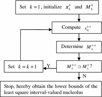

  

  Algorithm for determining nonnegativity of the lower bounds of the least square interval-valued nucleolus

Analogously, we can propose Algorithm 2 for determining nonnegativity of the upper bounds of the least square interval-valued nucleolus of the interval-valued cooperative game $\bar{\upsilon }$ as follows:

• Step 1: Set $k = 1$. Let $\varvec{x}_{R}^{k} = \varvec{x}_{R}^{{ * {\text{E}}}}$, where $\varvec{x}_{R}^{{ * {\text{E}}}} = (x_{R1}^{{ * {\text{E}}}} ,x_{R2}^{{ * {\text{E}}}} ,\cdots ,x_{Rn}^{{ * {\text{E}}}} )^{\text{T}}$ is the upper bound vector of the least square interval-valued prenucleolus of the interval-valued cooperative game $\bar{\upsilon }$, which is given by Eq. (28) (or generated by solving Eq. (33)). Let $M_{R}^{k} = \{ j \in N|x_{Rj}^{k} < 0\}$, which is the set of the players who have negative upper bounds of the interval-valued payoff vector $\varvec{x}_{R}^{k}$.

• Step 2: Compute

• $$ x_{Rj}^{k + 1} = \left\{ {\begin{array}{*{20}l} {x_{Rj}^{k} + \frac{{x_{R}^{k} (M_{R}^{k} )}}{{n - m_{R}^{k} }}} \hfill & { (j \notin M_{R}^{k} )} \hfill \\ 0 \hfill & { (j \in M_{R}^{k} ) ,} \hfill \\ \end{array} } \right. $$

• where $m_{R}^{k}$ is the cardinality of the player set $M_{R}^{k}$, i.e., $m_{R}^{k} = |M_{R}^{k} |$.

• Step 3: Let $M_{R}^{k + 1} = M_{R}^{k} \cup \{ j \in N|x_{Rj}^{k + 1} < 0\}$, which is the new set of the players who have negative upper bounds of the interval-valued payoff vector $\varvec{x}_{R}^{k + 1}$.

• Step 4: If $M_{R}^{k + 1} \supset M_{R}^{k}$, then set $k = k + 1$ and return to Step 2; If $M_{R}^{k + 1} = M_{R}^{k}$, then the solving process stops, hereby we can obtain the upper bounds of the least square interval-valued nucleolus of the interval-valued cooperative game $\bar{\upsilon }$, depicted as in Fig. 2.

  Fig. 2.

  

  Algorithm for determining nonnegativity of the upper bounds of the least square interval-valued nucleolus

From the above discussion, we can propose Algorithm 3 for computing the least square interval-valued nucleolus of any interval-valued cooperative game $\bar{\upsilon }$, depicted as in Fig. 3.

Fig. 3.

Algorithm 3 for computing the least square interval-valued nucleolus

In the following, we discuss some important and useful properties of the least square interval-valued nucleolus of any interval-valued cooperative game.

Theorem 7.

Assume that $\bar{\upsilon }$ is any interval-valued cooperative game. Then, there exists a unique least square interval-valued nucleolus, which satisfies the efficiency, individual rationality, additivity, symmetry, and anonymity.

Proof.

It is easy to prove Theorem 7 in a similar way to Theorems 2–6 and combining with Algorithms 1 and 2 (omitted).

6 A Numerical Example of Joint Production Problems

The following is an example how interval-valued cooperative games are applied to solve joint production problems.

Let us consider a joint production problem in which five decision makers actively cooperate with one another to develop new products. The five decision makers are named players 1, 2, 3, 4, and 5, respectively. Denoted the set of players by $N^{\prime} = \{ 1,2,3,4,5\}$. Before the cooperation starts, it is necessary for the five players (i.e., decision makers) to evaluate the revenue of the joint production project in order to decide whether the coalitions can be formed. However, the cooperative profit is dependent on many factors such as cost of human resources, product price, supply, and demand. Usually, players may estimate ranges of their profits instead of precisely forecasting their profits. Namely, the profit of a coalition $S\, \subseteq \,N^{\prime}$ of the players may be expressed with an interval $\bar{\upsilon }^{\prime}(S) = [\upsilon^{\prime}_{L} (S),\upsilon^{\prime}_{R} (S)]$. In this case, the optimal allocation of profits for the five decision makers may be regarded as an interval-valued cooperative game $\bar{\upsilon }^{\prime}$ in which the interval-valued characteristic function is equal to $\bar{\upsilon }^{\prime}(S)$ for any coalition $S\, \subseteq \,N^{\prime}$.

For example, let us consider a specific interval-valued cooperative game $\bar{\upsilon }^{\prime}$ which is defined as follows: $\bar{\upsilon }^{\prime}(2,3) = \bar{\upsilon }^{\prime}(2,4) = \bar{\upsilon }^{\prime}(3,4) = \bar{\upsilon }^{\prime}(3,5) = \bar{\upsilon }^{\prime}(4,5) = [100,200]$, $\bar{\upsilon }^{\prime}(1,3,4) = \bar{\upsilon }^{\prime}(1,3,5) = \bar{\upsilon }^{\prime}(1,4,5) = \bar{\upsilon }^{\prime}(2,3,5) = \bar{\upsilon }^{\prime}(2,4,5) = [100,200]$, $\bar{\upsilon }^{\prime}(2,3,4) = [120,240]$, $\bar{\upsilon }^{\prime}(3,4,5) = [175,300]$, $\bar{\upsilon }^{\prime}(1,2,3,4) = [175,350]$, $\bar{\upsilon }^{\prime}(1,2,3,5) = [100,220]$, $\bar{\upsilon }^{\prime}(1,2,4,5) = [100,250]$, $\bar{\upsilon }^{\prime}(1,3,4,5) = [200,380]$, $\bar{\upsilon }^{\prime}(2,3,4,5) = [200,400]$, $\bar{\upsilon }^{\prime}(1,2,3,4,5) = [200,600]$, and otherwise $\bar{\upsilon }^{\prime}(S) = 0.$.

Using Eq. (27), we can obtain the lower bounds of the least square interval-valued prenucleolus of the interval-valued cooperative game $\bar{\upsilon }^{\prime}$ as follows:

$$ x_{L1}^{{ * {\text{E}}}} = \frac{{\upsilon_{L} (N^{\prime})}}{5} + \frac{1}{{5 \times 2^{5 - 2} }}(5a_{L1} (\upsilon ) - \sum\limits_{{j \in N^{\prime}}} {a_{Lj} (\upsilon )} ) = \frac{200}{5} + \frac{1}{5 \times 8}(5 \times 1075 - 7485) = - 12.75, $$

$$ x_{L2}^{{ * {\text{E}}}} = \frac{{\upsilon_{L} (N^{\prime})}}{5} + \frac{1}{{5 \times 2^{5 - 2} }}(5a_{L2} (\upsilon ) - \sum\limits_{{j \in N^{\prime}}} {a_{Lj} (\upsilon )} ) = \frac{200}{5} + \frac{1}{5 \times 8}(5 \times 1295 - 7485) = 14.75, $$

$$ x_{L3}^{{ * {\text{E}}}} = \frac{{\upsilon_{L} (N^{\prime})}}{5} + \frac{1}{{5 \times 2^{5 - 2} }}(5a_{L3} (\upsilon ) - \sum\limits_{{j \in N^{\prime}}} {a_{Lj} (\upsilon )} ) = \frac{200}{5} + \frac{1}{5 \times 8}(5 \times 1770 - 7485) = 74.125, $$

$$ x_{L4}^{{ * {\text{E}}}} = \frac{{\upsilon_{L} (N^{\prime})}}{5} + \frac{1}{{5 \times 2^{5 - 2} }}(5a_{L4} (\upsilon ) - \sum\limits_{{j \in N^{\prime}}} {a_{Lj} (\upsilon )} ) = \frac{200}{5} + \frac{1}{5 \times 8}(5 \times 1770 - 7485) = 74.125, $$

and

$$ x_{L5}^{{ * {\text{E}}}} = \frac{{\upsilon_{L} (N^{\prime})}}{5} + \frac{1}{{5 \times 2^{5 - 2} }}(5a_{L5} (\upsilon ) - \sum\limits_{{j \in N^{\prime}}} {a_{Lj} (\upsilon )} ) = \frac{200}{5} + \frac{1}{5 \times 8}(5 \times 1575 - 7485) = 49.75, $$

respectively.

According to Algorithm 1, it is obvious that

$$ \varvec{x}_{L}^{1} = \varvec{x}_{L}^{{ * {\text{E}}}} = (x_{L1}^{{ * {\text{E}}}} ,x_{L2}^{{ * {\text{E}}}} ,x_{L3}^{{ * {\text{E}}}} ,x_{L4}^{{ * {\text{E}}}} ,x_{L5}^{{ * {\text{E}}}} )^{\text{T}} = ( - 12.75,14.75,74.125,74.125,49.75)^{\text{T}} . $$

Then, we give 0 to player 1 and divide $- 12.75$ equally among players 2, 3, 4, and 5. Hereby, we obtain

$$ \varvec{x}_{L}^{2} = (x_{L1}^{2} ,x_{L2}^{2} ,x_{L3}^{2} ,x_{L4}^{2} ,x_{L5}^{2} )^{\text{T}} = (0,11.5625,70.9375,70.9375,46.5625)^{\text{T}} $$

Thus, we finally obtain the lower bounds of the least square interval-valued nucleolus for the interval-valued cooperative game $\bar{\upsilon }^{\prime}$, i.e.,

$$ \varvec{x}_{L}^{{ * {\text{n}}}} = (0,11.5625,70.9375,70.9375,46.5625)^{\text{T}} . $$

Likewise, according to Eq. (28), we can obtain the upper bounds of the least square interval-valued prenucleolus of the interval-valued cooperative game $\bar{\upsilon }^{\prime}$ as follows:

$$ \varvec{x}_{R}^{{ * {\text{E}}}} = (19.5,77,180.75,184.5,138.25)^{\text{T}} . $$

Then, using Algorithm 2, we can obtain

$$ \varvec{x}_{R}^{1} = \varvec{x}_{R}^{{ * {\text{E}}}} = (19.5,77,180.75,184.5,138.25)^{\text{T}} . $$

Owing to the fact that all $x_{Ri}^{ 1}$ ($i \in N^{\prime}$) are nonnegative, we directly have

$$ \varvec{x}_{R}^{{ * {\text{n}}}} = \varvec{x}_{R}^{1} = (19.5,77,180.75,184.5,138.25)^{\text{T}} , $$

which is the upper bounds of the least square interval-valued nucleolus for the interval-valued cooperative game $\bar{\upsilon }^{\prime}$.

Therefore, we can obtain the least square interval-valued nucleolus of the interval-valued cooperative game $\bar{\upsilon }^{\prime}$ as follows:

$$ \bar{\varvec{x}}^{{*{\text{n}}}} = ([0,19.5],[11.5625,77],[70.9375,180.75],[70.9375,184.5],[46.5625,138.25])^{\text{T}} , $$

which may be interpreted as follows: player 1 can obtain at least 0 and at most 19.5, i.e., the interval $[0,19.5]$, which is almost greater than the interval $\bar{\upsilon }^{\prime}(1) = [0,0]$ obtained by itself alone. Analogously, player 2 can obtain at least 11.5625 and at most 77, i.e., the interval $[11.5625,77]$, which is obviously greater than the interval $\bar{\upsilon }^{\prime}(2) = [0,0]$ obtained by itself alone. Player 3 can obtain at least 70.9375 and at most 180.75, i.e., the interval $[70.9375,180.75]$, which is remarkably greater than the interval $\bar{\upsilon }^{\prime}(3) = [0,0]$ obtained by itself alone. The similar explanation can be done for players 4 and 5. In other words, the optimal allocations of all the five players $i$ ($i \in N^{\prime}$) satisfy the individual rationality of interval-valued payoff vectors according to Eq. (3), which is the Moore’s order relation over intervals [8].

Obviously, we have

$$ \sum\limits_{i = 1}^{5} {x_{Li}^{{ * {\text{n}}}} } = 0 + 11.5625 + 70.9375 + 70.9375 + 46.5625 = 200 $$

and

$$ \sum\limits_{i = 1}^{5} {x_{Ri}^{{ * {\text{n}}}} } = 19.5 + 77 + 180.75 + 184.5 + 138.25 = 600. $$

Hence,

$$ \sum\limits_{i = 1}^{5} {x_{i}^{{ * {\text{n}}}} } = \bar{\upsilon }^{\prime}(N^{\prime}), $$

which implies that the least square interval-valued nucleolus $\bar{\varvec{x}}^{{*{\text{n}}}}$ satisfies the efficiency of interval-valued payoff vectors as expected.

7 Conclusions

We propose the quadratic programming model and algorithms for solving the least square interval-valued nucleoli of interval-valued cooperative games and effectively avoid the magnification of uncertainty resulted from the Moore’s interval subtraction. The developed model and algorithms are simple and effective from the viewpoint of computational complexity. In addition, it is easy to see that the least square interval-valued prenucleoli and nucleoli of interval-valued cooperative games are generalizations of the least square prenucleoli and nucleoli for classical cooperative games.

However, only interval uncertainty is taken into consideration in coalition’s values in this paper. In fact, uncertainty of coalition’s values may be described by other types of data such as fuzzy numbers [17] and intuitionistic fuzzy numbers [18, 19]. Therefore, cooperative games with coalition values expressed by fuzzy numbers and intuitionistic fuzzy numbers will be hot topics in further research. What is more, the axiomatic characterizations of these types of cooperative games will also become hot issues of research.

References

Branzei, R., Branzei, O., Alparslan Gök, S.Z., Tijs, S.: Cooperative interval games: a survey. CEJOR 18, 397–411 (2010)
Li, D.-F.: Models and Methods for Interval-Valued Cooperative Games in Economic Management. Springer, Cham (2016). doi:10.1007/978-3-319-28998-4
Branzei, R., Dimitrov, D., Tijs, S.: Shapley-like values for interval bankruptcy games. Econ. Bull. 3, 1–8 (2003)
Alparslan Gök, S.Z., Branzei, R., Tijs, S.: The interval Shapley value: an axiomatization. CEJOR 18, 131–140 (2010)
Alparslan Gök, S.Z., Palanci, O., Olgun, M.O.: Cooperative interval games: mountain situations with interval data. J. Comput. Appl. Math. 259, 622–632 (2014)
Kimms, A., Drechsel, J.: Cost sharing under uncertainty: an algorithmic approach to cooperative interval-valued games. Bus. Res. 2, 206–213 (2009)
Mallozzi, L., Scalzo, V., Tijs, S.: Fuzzy interval cooperative games. Fuzzy Sets Syst. 165, 98–105 (2011)
Moore, R.: Methods and Applications of Interval Analysis. SIAM Studies in Applied Mathematics, Philadelphia (1979)
Hong, F.-X., Li, D.-F.: Nonlinear programming method for interval-valued n-person cooperative games. Oper. Res. Int. J. (2016). doi:10.1007/s12351-016-0233-1
Branzei, R., Alparslan Gök, S.Z., Branzei, O.: Cooperation games under interval uncertainty: on the convexity of the interval undominated cores. CEJOR 19, 523–532 (2011)
Alparslan Gök, S.Z., Branzei, O., Branzei, R., Tijs, S.: Set-valued solution concepts using interval-type payoffs for interval games. J. Math. Econ. 47, 621–626 (2011)
Alparslan Gök, S.Z., Miquel, S., Tijs, S.: Cooperation under interval uncertainty. Math. Methods Oper. Res. 69, 99–109 (2009)
Li, D.-F.: Linear programming approach to solve interval-valued matrix games. Omega Int. J. Manag. Sci. 39(6), 655–666 (2011)
Li, D.-F.: Fuzzy Multiobjective Many-Person Decision Makings and Games. National Defense Industry Press, Beijing (2003). (in Chinese)
Schmeidler, D.: The nucleolus of a characteristic function game. SIAM J. Appl. Math. 17(6), 1163–1170 (1969)
Ruiz, L.M., Valenciano, F., Zarzuelo, J.M.: The least square prenucleolus and the least square nucleolus: two values for TU games based on the excess vector. Int. J. Game Theor. 25(1), 113–134 (1996)
Li, D.-F., Hong, F.-X.: Solving constrained matrix games with payoffs of triangular fuzzy numbers. Comput. Math Appl. 64, 432–446 (2012)
Verma, T., Kumar, A., Appadoo, S.S.: Modified difference-index based ranking bilinear programming approach to solving bimatrix games with payoffs of trapezoidal intuitionistic fuzzy numbers. J. Intell. Fuzzy Syst. 29, 1607–1618 (2015)
Li, D.-F.: Decision and Game Theory in Management with Intuitionistic Fuzzy Sets. SFSC, vol. 308. Springer, Heidelberg (2014). doi:10.1007/978-3-642-40712-3
Author information
Authors and Affiliations
Corresponding author
Editor information
Editors and Affiliations
Rights and permissions
Copyright information
© 2017 Springer Nature Singapore Pte Ltd.
About this paper
Cite this paper
Li, WL. (2017). Models and Algorithms for Least Square Interval-Valued Nucleoli of Cooperative Games with Interval-Valued Payoffs. In: Li, DF., Yang, XG., Uetz, M., Xu, GJ. (eds) Game Theory and Applications. China GTA China-Dutch GTA 2016 2016. Communications in Computer and Information Science, vol 758. Springer, Singapore. https://doi.org/10.1007/978-981-10-6753-2_21
Download citation
DOI: https://doi.org/10.1007/978-981-10-6753-2_21
Published:
Publisher Name: Springer, Singapore
Print ISBN: 978-981-10-6752-5
Online ISBN: 978-981-10-6753-2
eBook Packages: Computer ScienceComputer Science (R0)