Computer-Assisted Treatment Planning Approaches for Carbon-Ion Beam Therapy

Abstract

In this chapter, we introduced the basic concept of the charged particle beam therapy from a physics point of view. Although treatment procedures for particle beam therapy are closely similar to those for the photon beam therapy, beam range (penetration depth) should be taken into account carefully in the particle beam therapy due to different characteristics of them. Moreover, heavy charged particle beam leads to complex biological effect compared to proton beam. For readers not familiar with charged particle beam therapy, therefore, we provide the sufficient information of the particle therapy physics and its clinical application.

1 Introduction

State-of-the-art radiotherapy techniques improve dose conformation to the target and dose sparing to normal tissues compared to conventional methods. These precise delivery techniques, which include intensity-modulated radiotherapy (IMRT) and volumetric modulated arc therapy (VMAT) in the photon world and intensity-modulated particle therapy (IMPT) in the particle world, allow much steeper dose gradients between the target region and surrounding healthy tissue. The physics of interactions differ between charged particle and photon beams, one result of which is that particle beam therapy reduces excessive dose to healthy tissues and maintains a high target dose, leading to good tumor control rates with less toxicity and improved patient quality of life (Fig. 7.1). Those unfamiliar with particle beam treatment might feel that charged particle beam treatment planning is both difficult and markedly different from photon beam treatment planning. But as noted by Dr. Goitein at the Particle Therapy Co-Operative Group (PTCOG) meeting in 2006 (Goitein 2006), they share most of the same treatment planning procedures and primarily differ only in particle beam’s finite penetration and sensitivity to tissue density variation along a given ray. Moreover, treatment planning for heavy charged particle beams (commonly used to characterize ions heavier than protons) should take account of the nonlinear additivity of the biologically weighted dose. The more precise beam delivery and treatment planning techniques developed recently require image guidance, which provides visualization and quantification of patient geometrical information from medical images and improves treatment workflow.

Fig. 7.1

Dose distribution with passive scattering carbon-ion radiotherapy (CIRT) (upper panel) and IMRT (lower panel). Yellow arrows show beam fields (With permission from Tsujii et al. 2014)

In this chapter, we introduce basic concepts of carbon-ion beam treatment planning with image guidance/image processing (in a sense, image-guided particle therapy, IGPT) and emphasize the differences between particle beam therapy and photon beam therapy. Several recent articles on particle beam therapy provide important additional skill-building information (Jakel et al. 2008; Tsujii and Kamada 2012; Chen et al. 2009, 2006).

2 Why Choose Carbon Ions?

It is well known that the high energy of a therapeutic photon beam decreases in a steep exponential curve with penetration depth and that the dose close to the entrance surface shows “buildup” caused by forward-scattered Compton electrons. In contrast, charged particle beams provide superior dose conformation to photon beams and minimize excessive dose to normal tissues. These strengths owe to the characteristic increase in energy deposition of particle beams with penetration depth (proton and carbon-ion beams) up to a sharp maximum at the end of the beam range (Bragg peak) (Fig. 7.2) (Bragg and Kleeman 1904). Explained simply, accelerated particle beam interactions lose kinetic energy along the ray line due to the interaction of Coulomb forces with the target electrons (stopping power). This is expressed by the Bethe-Bloch formula. Stopping power is approximately proportional to (Z/v)²:

$$ \frac{\mathrm{d} E}{\mathrm{d} x}\sim \frac{Kn{\mathrm{Z}}^2}{v^2}\ \left[ \ln \left(\frac{2{m}_e{v}^2}{I}\right)\right]\propto {\left(\frac{\mathrm{Z}}{v}\right)}^2, $$

(7.1)

where K, n, and m _e are the constant, electron density of the target material, and mass of electrons, respectively. Z is the charge of the projectile particle, v is the projectile velocity, and I is the mean ionization energy of the target atoms.

Fig. 7.2

Depth absorbed dose distributions of (a) a primary proton beam and its secondary particles and (b) a carbon-ion beam and its secondary particles (Reproduced from Kempe et al. 2007)

Accordingly, projectile velocity slows down as material penetration deepens, and stopping power is increased. Projectile velocity at the end of range is close to zero, and a high dose is deposited there.

In 1975–1992, neon ions and helium ions were used to treat 433 cancer patients and 2054 patients, respectively, at the Lawrence Berkeley National Laboratory (Alonso 2000), while in 1994, the heavy ion medical accelerator (HIMAC) at the National Institute of Radiological Sciences (NIRS) began providing carbon-ion radiotherapy (CIRT). From clinical experience gained at Berkeley, most heavy charged particle beam centers have selected carbon ions, mainly for the following reasons:

• 1. Ions heavier than carbon have an increased nuclear fragmentation tail dose.

  Protons did not deposit dose beyond the Bragg peak (Fig. 7.2a). In contrast, ions heavier than protons still had low projectile energy nuclear interactions (elastic collisions with target nuclei), providing a small dose (fragment particles with lower atomic number) beyond the Bragg peak (Fig. 7.2b).

• 2. Ions heavier than carbon increase LET and relative biological effectiveness (RBE).

  Conceptually, RBE represents the particle beam dose which provides the same biological effect as would be provided by the reference dose (typically X-rays or γ-rays). The RBE of light ions (proton, helium, etc.) does not significantly change between the entrance region and distal spread-out Bragg peak (SOBP) (Fig. 7.3). In contrast, the RBE of carbon ions is similar to that of light ions at the proximal SOBP but increased at the distal SOBP. The light-ion relative biological dose at the plateau region is therefore higher than the carbon-ion relative biological dose (Fig. 7.4). In contrast, the RBE of heavier ions (neon, argon, etc.) at the proximal and distal SOBPs is higher than that of carbon ions (although the RBE of neon at the entrance region is smaller than that of carbon ions at the distal SOBP). Although the relative biological dose of heavier ions at the SOBP is the same as that of carbon ions, the relative biological dose at the entrance region and proximal and distal SOBPs is higher than that of carbon ions. As a result, the peak to plateau ratio for carbon ions is higher and therefore improved, over that of other particle beams, including protons.

  Fig. 7.3

  

  Relative biological effectiveness (RBE) of different ions in fractionated irradiation of jejunal crypt cells of mice (With permission from Jakel 2009)

  Fig. 7.4

  

  Relative biological dose of the SOBP of ion beams. Doses are normalized at the SOBP region (With permission by the IAEA 2007)

• 3. Heavier ions minimize the magnitude of range straggling and lateral scattering.

  These factors blur out the sharp ionization peak. Range straggling causes smearing out of the depth of penetration of the stopping particle beam due to statistical fluctuations in the ionization process. The variance of the range straggling is expressed from Bohr’s theory as follows:

$$ \varphi (x)=\frac{1}{\sigma_x\sqrt{2\pi}} \exp \left(\frac{-{\left( x- R(E)\right)}^2}{2{\sigma}_x^2}\right), $$

(7.2)

$$ R(E)={\int}_0^E{\left(\frac{\mathrm{d} E\prime }{\mathrm{d} x}\right)}^{-1}\mathrm{d} E^{\prime }, $$

(7.3)

• where x is the penetration depth, σ _x is almost proportional to range R and inverse to the square root of the particle mass, and range straggling for helium and neon are about 50 and 20 % of that for protons, respectively. Lateral scattering is mainly caused by elastic Coulomb interactions with the target nuclei and can be approximated by Gaussian functions as follows (Highland 1975):

$$ {\sigma}_{\theta}=\frac{14.1\mathrm{MeV}}{\beta pc}{Z}_p\sqrt{\frac{d}{L}}\left[1+\frac{1}{9}{ \log}_{10}\left(\frac{d}{L}\right)\right], $$

(7.4)

• where L and d are the radiation length and penetration length, respectively, β is particle beam velocity, and p and c are the momentum of the incident particle and the speed of light, respectively. The magnitude of the lateral scattering of photons and protons is larger than that for carbon ions at the same depth (Fig. 7.5).

  Fig. 7.5

  

  Lateral scattering of photon, proton, and carbon-ion beams as a function of penetration depth (With permission from Kraft 2000)

• 4. Heavier ions require a large accelerator.

  Due to differences in their mass-to-charge ratio, it is two times more difficult to bend a carbon-ion beam with an accelerator than protons under same magnetic field, and the range of carbon ions is three time shorter than that of protons under the same velocity. Carbon-ion beams therefore require higher energy than protons to obtain the same range by enlarging accelerator size. Current particle beam center construction costs are dominated by size of the accelerator, which requires a large housing size. Progress in accelerator technology over the last 20 years has contributed to cost reductions by reducing accelerator size. For example, the cost of the synchrotron ring at Gunma University, which was constructed in 2009, was 63 m, approximately half that of the NIRS, constructed in 1993.

Given the above, it appears that carbon ions represent a well-balanced particle in both physical and biological aspects (Table 7.1). In 2015, more than ten treatment centers were operating CIRT, as shown on the website of the PTCOG. The NIRS has treated over 8000 patients using carbon ions, and their clinical experience is reported here (Tsujii and Kamada 2012).

Table 7.1 Summary of the characteristics of particle beams

3 Particle Beam Treatment Planning

3.1 Planning CT

CT imaging provides both patient 3D anatomical information and effective density information, making it an essential part of treatment planning. This 3D information is markedly helpful in deciding treatment parameters, especially beam angle and dose distribution. An immobilization device is typically used in the planning CT acquisition and treatment stages to improve patient positional reproducibility throughout the treatment course. Several treatment centers have installed a large bore CT (over 80 cm diameter) to avoid the conflict between positioning of the raised arm and immobilization which occurs with a standard bore CT (about 72 cm diameter).

Recent commercial CT scanners are equipped with a 4D mode to capture respiratory-induced organ motion. 4DCT is a breakthrough technique which allows the quantification of intrafractional uncertainties. This technique is applied in cardiac CT imaging and has already become practical for identifying patients with significant coronary artery stenosis by ECG-correlated preprocessing. Given the heartbeat (~ 1 s) is faster than respiratory motion (~ 4 s) and coronary arteries (~ a few mm) are smaller than lung tumors (~ a few cm), it should therefore be feasible to visualize intrafractional motion. Although the respiratory pattern shows variations (e.g., phase shift/drift), 4DCT scans provide information of a single exemplary respiratory cycle only. Thus, serial CT/4DCT image acquisition is performed over a certain time axis (daily, weekly, etc.) to obtain potential anatomical changes. This information can be helpful in considering replanning during the treatment course.

In photon beam therapy, megavoltage X-ray interaction in material is dominated by Compton scattering, and effective density is calibrated using relative electron density. Typically, HU (Hounsfield unit) values within the patient are measured by the planning CT image and converted to linear attenuation coefficients (μ):

$$ \mu =\left( HU-{HU}_{\mathrm{air}}\right){\left({HU_{\mathrm{water}}- HU}_{\mathrm{air}}\right)}^{-1}, $$

(7.5)

The linear attenuation coefficient is derived from the formula or photon attenuation (Rutherford et al. 1976):

$$ \mu ={\rho}_e\left({K}^{\mathrm{ph}}{Z}^{3.62}+{K}^{\mathrm{coh}}{Z}^{1.86}+{K}^{\mathrm{KN}}\right), $$

(7.6)

where K ^ph, K ^coh, and K ^KN are constants for the contribution of the photoelectric effect, coherent scattering, and Compton scattering, respectively.

Particle beam ranges in materials are scaled by the stopping-power ratio relative to water based on measurement in water during beam commissioning. Accordingly, effective density in charged particle beams should be defined as the stopping power relative to water (ρ _s ):

$$ {\rho}_s={\rho}_e\left[ \ln \left(\frac{2{m}_e{c}^2}{I_{\mathrm{material}}}\frac{\beta^2}{1-{\beta}^2}\right)-{\beta}^2\right]{\left[ \ln \left(\frac{2{m}_e{c}^2}{I_{\mathrm{water}}}\frac{\beta^2}{1-{\beta}^2}\right)-{\beta}^2\right]}^{-1}, $$

(7.7)

where ρ _e and m _e are relative electron density and the electron mass, respectively, and I _material and I _water are the mean ionization energies in material and water, respectively. Several carbon-ion beam treatment centers in Japan use CT calibration using the polybinary tissue model (muscle (water), air, fat (ethanol), and bone (40 % K₂HPO₄ water)) due to the good balance it provides between quality and cost (Kanematsu et al. 2003). By doing this, dose distribution can be calculated by converting all CT image sets to the effective density in the treatment planning system (TPS).

3.2 Contouring

3.2.1 Volume of Interest (VOI)

Since the planning CT image contains patient anatomical information that the TPS does not recognize, the volume of interest (VOI) on the CT image should be input into the TPS to conform the prescribed dose to the tumor and to minimize dose to normal tissues. The International Commission on Radiation Units and Measurement (ICRU) first defined the VOI in ICRU report 50 (1993) and refined it further in ICRU reports 62 (1999), 71 (2005), and 78 (2007). These VOI terms are illustrated in Fig. 7.6, in which the target-related terms are gross tumor volume (GTV), clinical target volume (CTV), internal target volume (ITV), and planning target volume (PTV). The term “target volume” is often used for both target and healthy tissues but is more specific to the tumor. We therefore use VOI here to describe both tumor and normal tissues. Although the VOI is fully defined in these ICRU reports, I introduce it briefly here as follows.

Fig. 7.6

Schematic drawing of the volumes of interest relating to the definition of target and organs at risk

The GTV consists of a primary/metastatic tumor and demonstrable visible tumor region on planning images. It is generally delineated by the oncologist and may not be present following irradiation treatment. The CTV contains the GTV and subclinical malignant disease region (microscopic tumor spread region), which in some cases is difficult to observe in the planning CT image. To compensate for expected internal uncertainties such as physiologic movement and temporal size/shape/positional variations, the ITV is defined by adding an internal margin to the CTV. This internal margin technique is often used in thoracoabdominal treatment. The PTV is designed by adding a setup margin to the ITV. This setup margin accounts for the inaccuracy and low reproducibility of patient positioning to the treatment beam. The PTV in photon beam therapy generally uses the geometrical-based margins of the beam field to compensate for organ motion and setup errors. Since particle beam therapy considers uncertainties in beam penetration, the PTV should include the range-based proximal and distal margins of the beam field as well as the lateral margins. The PTV is therefore designed for each beam direction. The margin for respiratory-induced range uncertainties is described in Sect. 7.4.

In addition, critical normal structures (organs at risk, OARs) are also delineated on the TPS. Because OARs are likely affected by intra-/interfractional movement, patient setup error, etc., planning organ at risk volume (PRV) is delineated in addition to the ITV and PTV concepts by adding an internal margin and setup margin to OARs (Fig. 7.6). In some cases, the PTV overlaps another PTV, OAR, or PRV; however, ICRU reports 78 and 83 recommend that delineating the VOIs should not be compromised because recent TPS can optimize sufficient dose sparing of the OAR. As described here, GTV, CTV, and OAR are oncological or anatomical concepts, while ITV, PTV, and PRV are physical constructions.

3.2.2 Image Registration/Segmentation

The image registration/segmentation technique is mandatory in current radiotherapy procedures, particularly in treatment planning. Generally, image registration is used for contouring and 4D dose calculation. The latter is described in Sect. 7.4. Image segmentation supports the inputting of target and normal organ contours automatically (auto-contouring) without a huge burden on the oncologist. In contrast, image registration is used to transform contours between different CT data sets for the same patient and in replanning (from original CT to new CT) and 4DCT (from a reference phase to other phases). Deformable image registration (DIR) is used in place of rigid image registration to reflect realistic human geometrical changes. In treatment planning, multiple sets of image data (CT, MRI, PET, and their combinations) are generally registered. The DIR process finds a deformation vector field (DVF) between two image data sets.

DVF is obtained by applying a transforming function (generally B-spline with control points) to the reference image and calculating similarity measure between the two images. This process is repeated until the similarity measure reaches the criterion value. When the same imaging modality data set is used, image voxel values for each image data set are similar; therefore, to avoid the time-consuming in user input of further information, the intensity-based DIR method is more suitable than the landmark-based or segmentation-based methods, because it operates on image voxel values directly. Voxel similarity measure generally uses sum of squared differences and cross correlation etc.; these contours are transferred to the next image data set by applying DVF to the contours on the reference image (warping). As an example of auto-contouring in 4DCT, an oncologist manually contours one reference CT phase (generally peak exhalation), and then DIR calculates the DVF based on the 4DCT data. These are then applied to the manual contours to transform them from the reference phase to the other respiratory phases. All contours at other respiratory phases are then automatically calculated.

DIR-related auto-contouring and 4D dose calculation (described later) can have a significant impact on treatment accuracy. It is therefore important to assess registration accuracy, which is strongly dependent on patient shape. Accordingly, it is not sufficient to evaluate the registration accuracy using a phantom only.

A simple evaluation method for the registrations is visual assessment. Point landmark-based registration is performed to obtain a quantitative result, but it is substantially time-consuming and not practical in clinical settings. It is necessary to check DIR accuracy from the CT image at exhale (IM_exhale) to that at inhale (IM_inhale):

$$ {{\mathrm{IM}}_{\mathrm{exhale}}:{\boldsymbol{x}}_{\mathrm{exhale}}\in {\Omega}_{\mathrm{exhale}},\kern0.5em \mathrm{IM}}_{\mathrm{inhale}}:{\boldsymbol{x}}_{\mathrm{inhale}}\in {\Omega}_{\mathrm{inhale}}, $$

(7.8)

where Ω_exhale and Ω_inhale are discrete domains of CT images at exhale and inhale and x_exhale and x_inhale are position vectors on CT images at exhale and inhale, respectively. Subtracted CT images at inhale and exhale show large differences in voxel values due to geometrical differences (Fig. 7.7a). DVF is calculated using CT images at exhale and inhale:

$$ \mathrm{DVF}:{\Omega}_{\mathrm{exhale}}\to {\Omega}_{\mathrm{inhale}}, $$

(7.9)

A warped CT image at inhale is calculated by applying DVF to the CT image at exhale. If the registration error is zero, the warped CT image and CT image at inhale are the same:

$$ {\boldsymbol{x}}_{\mathrm{inhale}}=\mathrm{DVF}\left({x}_{\mathrm{exhale}}\right), $$

(7.10)

Geometrical differences between the warped CT image and CT image at inhale are improved (Fig. 7.7b), but the registration error is not completely zero when using patient images:

$$ {\boldsymbol{x}}_{\mathrm{inhale}}\ne \mathrm{DVF}\left({x}_{\mathrm{exhale}}\right), $$

(7.11)

We then calculated another DVF (DVF’) by using the warped CT image at exhale and CT image at inhale and applied DVF’ to the warped CT image (${\overset{\sim }{IM}}_{exhale}$):

$$ \overset{\sim }{\mathrm{DVF}}:{\Omega}_{\mathrm{exhale}}^{\mathrm{DVF}}\to {\Omega}_{\mathrm{inhale}}, $$

(7.12)

$$ {\overset{\sim }{\mathrm{IM}}}_{\mathrm{exhale}}:{\overset{\sim }{\boldsymbol{x}}}_{\mathrm{exhale}}\in {\Omega}_{\mathrm{exhale}}^{\overset{\sim }{\mathrm{DVF}}}, $$

(7.13)

$$ {\overset{\sim }{\boldsymbol{x}}}_{\mathrm{exhale}}=\overset{\sim }{\mathrm{DVF}}\left[\mathrm{DVF}\left({x}_{\mathrm{exhale}}\right)\right], $$

(7.14)

DIR accuracy is quantitatively visualized by the following calculation (Fig. 7.7c):

$$ {\left\Vert \overset{\sim }{\mathrm{DVF}}\left({\overset{\sim }{\boldsymbol{x}}}_{\mathrm{exhale}}\right)-{\boldsymbol{x}}_{\mathrm{inhale}}\right\Vert}_2, $$

(7.15)

where ‖∙‖ represents a norm.

Fig. 7.7

(a) Subtraction CT image at inhale from that at exhale. (b) Subtraction CT image at inhale from warped CT at inhale. (c) Magnitude of the DVF color map between CT image at inhale and warped CT image at inhale

Image registration which utilizes DIR cannot remove registration error completely, and users should therefore check the contours and modify manually if necessary. In particular, a lung DIR close to the chest wall could degrade registration accuracy, because intrafractional chest wall movement is smaller than lung motion. Biomechanical intensity-based DIR considers physical properties and in one study improved target registration error, from 1.5 ± 1.4 mm (mean ± SD) compared with conventional DIR (2.6 ± 1.4 mm) (Samavati et al. 2015). The author does not provide details of the biomechanical DIR technique here, but note that it is strongly dependent on the DIR algorithm (Brock 2010). Details about image registration can be found elsewhere (Hill et al. 2001).

3.3 Beam Angle Configuration

Conformal photon beam treatment planning such as IMRT generally uses more than six beam fields to reduce the doses to normal tissues, while VMAT delivers the treatment beam using a rotating gantry. The use of multiple beam fields might minimize dose errors. While a few beam fields provide good target dose conformity in particle beam therapy, dose error in respective fields should not be neglected. Given that current TPS are unable to select all beam angles automatically, treatment planners should select beam angles with consideration to the following:

• 1. Avoid beam angles along the target and OAR direction to spare OARs.

  This is easy to understand in the case of OARs located proximal to the target but should also be considered for OARs at the distal side. Ideally the particle beam stops at the distal edge of the target, but range uncertainty might change particle beam stopping position; an extended particle beam position might increase harmful dose to OARs located close behind the target.

• 2. Opposing beam angles achieve a good biologically effective dose.

  Since RBE values vary as a function of depth, opposing beam angles are not good for OAR sparing; except for tumors located around the body center, beam angles should be separated within the approximate range of 25° to 70° or something similar.

• 3. Avoid inhomogeneous tissue and consider patient positional variation to minimize range uncertainty.

  Small dose differences were observed between commercial TPS and Monte Carlo (MC)-derived planning, particularly for the skull and thoracic regions, which include inhomogeneous tissues (Fig. 7.8). This is because most TPSs use empirical models for dose calculation, despite the fact that the MC algorithm is much more accurate for dose calculation. Patient anatomical intra-/interfractional positional variation is a major factor in range uncertainty. An example of intrafractional beam range variation is that a single pencil beam stops at the distal edge of a tumor when passing through the heart at diastole but penetrates the tumor at systole (Fig. 7.9). Careful selection of beam angle is one solution to minimizing range uncertainties.

  Fig. 7.8

  

  Proton dose distribution calculated with a commercial TPS (XiO, Elekta Inc.) (left panel) and by Monte Carlo (MC) (right panel; Geant 4) (Adapted from Paganetti et.al. 2008)

  Fig. 7.9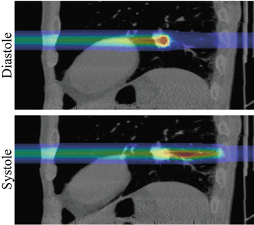

  

  Carbon-ion pencil beam dose distribution at diastole and systole

• 4. Consider positioning and irradiation systems restrictions.

  Photon beam and proton beam treatment use rotating gantry systems to irradiate from a wide range of gantry angle. However, carbon-ion beam rotating gantry systems have not been widely adopted, although a few have been constructed in Japan and Germany. These may allow the selection of beam angles which avoid the treatment couch edge. Since most CIRT centers use a fixed beam port irradiation system, extending the range of beam angles requires the treatment couch to be rotated around the patient long axis. Planners should leave this part in the tip of the corner.

3.4 Irradiation Method

This section provides a brief technical overview of the two most common irradiation techniques used in CIRT, passive scattering, and pencil beam scanning (PBS).

The passive scattering irradiation technique has been long and widely used in charged particle beam therapy, including proton and carbon-ion beams. A pristine beam with a narrow beam width in both lateral and depth directions is extracted from the accelerator. To cover the whole target volume, the pristine beam should be spread out in both directions. First, a wobbler magnet and scattering system are used to laterally and uniformly spread the pristine beam (Fig. 7.10a). Second, a ridge filter modulates the beam energy to obtain a uniform biological dose distribution along depth direction SOBP. Third, a patient collimator (PTC) and/or multi-leaf collimator (MLC) are used to adjust the beam to the target volume laterally. Finally, a compensator bolus adjusts the beam stopping position at the distal edge of the target. This method provides good dose conformity for the distal region of the target, but cannot avoid an unnecessarily high dose around the proximal side of the target.

Fig. 7.10

Schematic drawing of (a) passive scattering, (b) layer-stacking, and (c) scanning irradiation techniques. Dotted curved lines show the iso-energy layers

The layer-stacking irradiation technique was developed in 1983 with the aim of maximizing dose conformation and minimizing the dose to normal tissue around the proximal side of the target with scattering beams, similar to that with PBS irradiation. It is now in clinical use at a few carbon-ion beam treatment centers (Kanai et al. 1983; Kanematsu et al. 2002). Uniform dose within the target is achieved by combining a number of small SOBPs along a depth direction. These small SOBP positions are shifted by changing range shifters (Fig. 7.10b). Beam field size is defined to fit the respective iso-energy layer regions by changing the MLC opening width.

With regard to PBS, this method was first proposed in the 1980s at NIRS, and carbon-ion PBS (C-PBS) was first implemented clinically at the Gesellschaft für Schwerionenforschung (GSI) in Darmstadt, Germany (Kanai et al. 1980; Haberer et al. 1993). Worldwide, a few treatment centers were using C-PBS as of 2015. The pencil beam is scanned in all three dimensions over the spot positions of the target to achieve a uniform dose within the target (Fig. 7.10c). Since PBS has a flexible dose distribution, OAR sparing is better than with passive scattering irradiation, and an inhomogeneous dose distribution (e.g., IMPT, additional doses to hypoxic regions) can be achieved. MLC, PTC, and a compensator bolus are not required, eliminating the treatment workflow time normally required to change these accessories and minimizing therapist entry into the treatment room. The beam energy is changed with a range shifter and/or accelerator change. A major problem with the use of a thicker range shifter is that it causes a broadening of the beam spot size with increasing depth through range shifters. By contrast, active change using an accelerator takes energy change time and requires a massively extended commissioning time for each beam energy (over a few hundred beam energies). Hybrid depth scanning with a synchrotron was developed to overcome these problems. Hybrid depth scanning provides a smaller lateral dose fall off and RBE than range shifter scanning (Inaniwa et al. 2012) and uses the range shifter to shift the small SOBPs at a step size of 3 mm in combination with 11 distinct synchrotron energies (Fig. 7.11).

Fig. 7.11

C-PBS dose distributions in the depth direction (D_p), lateral direction (σ), and normalized fluence for RS, ES, and HS, respectively (With permission from Inaniwa et al. 2012)

3.5 Dose Calculations

3.5.1 Beam Range Calculation

Beam spot positions are set on steps of a few millimeters (generally 2–3 mm, depending on C-PBS beam size) on CT images. Water equivalent path length (WEPL) from the irradiation system (scanning magnet) to respective spots is calculated by integrating the stopping effective density along each ray line:

$$ \mathrm{WEPL}(z)={\int}_0^z{\rho}_s\left({z}^{\prime}\right)\mathrm{d} z^{\prime }, $$

(7.16)

where z is the total penetration depth, z’ is the penetration depth, and ρ _s is the stopping power.

For the square-shaped case in Fig. 7.12, the same WEPL position (iso-energy layer) (shown as dotted lines) is oriented in a horizontal line (Fig. 7.12a). Most distal spot positions (red circles in Fig. 7.12a) are irradiated by the same energy beam. For the spherically shaped case, in contrast, the iso-energy layer position is curved and not the same as the target shape (Fig. 7.12b). Most distal spot positions (red circles in Fig. 7.12b) are irradiated by different beam energies. In a more realistic case (lung case), the tissue density for lung may be decreased from approximately 1.0 g/cm³ to 0.3 g/cm³, potentially exerting a strong impact on the iso-energy layer position by making it more complex. To understand this more clearly, the lung CT image is transformed in the same WEPL value positions in Fig. 7.12d; compared to the original lung CT (Fig. 7.12c), the geometrical shape is substantially deformed, and the lung thickness is substantially shortened in the WEPL coordinate. C-PBS doses are calculated in respective beam spots.

Fig. 7.12

Schematic diagram of the beam spot position in several iso-energy layers for (a) rectangular shape and (b) spherical shape. Iso-energy layer number was assigned from the distal side (With permission from ICRU-72 2007). Lung CT images in coronal section in (c) CT and (d) WEPL coordinates

3.5.2 Beam Modeling

For the C-PBS beam model, lateral dose distribution can be approximated by the Gaussian function as a function of penetration depth. Accumulated dose distribution in the PBS irradiation is superimposed on the respective pencil beam dose distributions, meaning that beam field size would be varied at the respective iso-energy layers. The dependence of photon and particle beam doses on beam field size is well known and is likely emphasized in PBS irradiation. However, a single Gaussian model does not completely compensate for the field size effect. Proton beam lateral distribution can be expressed by the sum of two Gaussians: the first and second components are the primary proton and nuclear beam halo, respectively (Pedroni et al. 2005). For carbon-ion beams, three Gaussians are used to accurately model the lateral distributions on account of nuclear fragments; the first component is primary carbon ion, the second is heavy fragments, and the third is light fragments (Inaniwa et al. 2009; Kusano et al. 2007) (Fig. 7.13), and the ith PBS dose distribution (d _i (x,y,z)) is expressed by the following:

$$ \begin{array}{ll}{d}_i\left(x,y,z\right)=& {d}_{z,i}(z)\hfill \\ {}& \times \left\{\left(1-\sum_{j=2}^3{f}_{j,i}(z)\right){D}_{1,i}\left(x,y,{\sigma}_{1,i}(z)\right)+\sum_{j=2}^3{f}_{j,i}(z){D}_{j,i}\left(x,y,{\sigma}_{j,i}(z)\right)\right\}\kern0.5em ,\hfill \end{array} $$

(7.17)

where d _z.,i (z) and σ _j,i (z) are the integral dose and standard deviation at a penetration depth z, respectively; D _j,i (x,y, σ _j,i (z)) is a two-dimensional Gaussian function for the lateral distribution of the jth component; and f _j,i (z) is the fraction of integrated dose of the jth Gaussian component. Physical dose distribution for PBS (D _phys ) is composed by summing the respective pencil beam doses:

$$ {D}_{\mathrm{phys}}\left( x, y, z\right)=\sum_{i=1}^N{d}_i\left( x, y, z\right)\bullet {w}_i, $$

(7.18)

where N is the total number of spots and w _i is the ith beam spot weight.

Fig. 7.13

(a) Lateral beam spreads of the first, second, and third components for the range shifter thicknesses of 0, 50, and 100 mm WEL. (b) Fraction factors of the second and third components for the range shifter thicknesses of 0, 50, and 100 mm WEL (Reproduced from Inaniwa et al. 2009)

3.5.3 Biological and Clinical Doses

Since biological effect in heavy charged particle therapy is strongly dependent on particle type, the primary particle and all fragment particles produced during the stopping process should be considered (Schardt et al. 2010). To discriminate the physical dose (Gy), ICRU recommends use of the term “RBE-weighted” dose (Gy (RBE)) for biological dose (ICRU-72 2007). Biological dose distribution is expressed as a typical tumor cell response, as defined by the in vitro response of human salivary gland (HSG) tumor cells. A German group adapted the local effect model (LEM) to CIRT (Elsasser et al. 2008). Another model was introduced as the microdosimetric kinetic model (MKM), which predicts the survival fraction of cells from the specific energy absorbed by a microscopic subcellular structure (Hawkins 1996; Hawkins 2003). However, MKM does not perfectly predict RBE due to insufficient overkill correction in high-energy regions (LET >100 keV/μm). To solve this problem, Kase et al. adapted saturation correction to express the decrease in RBE due to the overkill effect in a mixed radiation field (modified MKM) (Kase et al. 2006b). The modified MKM provides RBE values from proton to silicon using a linear quadratic (LQ) function, which simplifies the calculation of RBE under the mixed radiation field (Kase et al. 2006a) (Fig. 7.14).

Fig. 7.14

Relationship between experimental α value and the saturation-corrected dose-mean lineal energy (With permission from Kase et al. 2006a)

Biological dose in the mixed radiation field is expressed as follows:

$$ {D}_{\mathrm{biol}}\left( x, y, z\right)={D}_{\mathrm{phys}}\left( x, y, z\right)\bullet {RBE}_{\mathrm{biol}}\left( x, y, z\right)=-\frac{\alpha}{2\beta}+\sqrt{{\left(\frac{\alpha}{2\beta}\right)}^2-\frac{ \ln S\left({D}_{\mathrm{phys}}\left( x, y, z\right)\right)}{\beta}}, $$

(7.19)

$$ \ln \left( S\left({D}_{\mathrm{phys}}\left( x, y, z\right)\right)\right)=-\left({\alpha}_0+\beta {z}_{1 D\ \mathrm{mix}}^{*}\left( x, y, z\right)\right){D}_{\mathrm{phys}}\left( x, y, z\right)-\beta {D_{\mathrm{phys}}\left( x, y, z\right)}^2, $$

(7.20)

where α and β are the coefficients of the LQ model for the reference radiation and α ₀ is the initial slope of the surviving fraction curve in the limit of LET = 0. β value is independent of radiation type and is selected as 0.0615Gy^-2 based on the β value of HSG cells irradiated by X-ray (Furusawa et al. 2000). To predict RBE in the mixed radiation field, the saturation-corrected dose means that a single energy extended to the saturation-corrected dose-mean specific energy (${z}_{1 D\ mix}^{*}$), which can be derived by MC and the Kiefer-Chatterjee model (Kiefer and Straaten 1986), must be calculated (Fig. 7.15). Details for calculating the saturation-corrected dose-mean specific energy are described in Inaniwa et al. (2010):

$$ {z}_{1 D\ \mathrm{mix}}^{*}\left( x, y, z\right)=\frac{\sum_{i=1}^N{w}_i\bullet {d}_i\left( x, y, z\right)\bullet {\overset{-}{z}}_{1 D: i}^{*}(z)}{\sum_{i=1}^N{w}_i\bullet {d}_i\left( x, y, z\right)}, $$

(7.21)

where ${\overset{-}{z}}_{1 D: i}^{*}(z)$ is the saturation-corrected dose-mean specific energy delivered by the jth beam. To adapt biological response in vitro to patient treatment (in vivo), the biological dose should be rescaled by multiplying by a clinical factor (F _clin). Clinical dose can be calculated by the following:

$$ {D}_{\mathrm{clin}}\left( x, y, z\right)={D}_{\mathrm{bio}}\left( x, y, z\right)\bullet {F}_{\mathrm{clin}}, $$

(7.22)

The clinical factor of 2.41 is used in our facility. Due to word count limitations, details and historical background are provided elsewhere (Kanematsu et al. 2002; Kanai et al. 1999; Inaniwa et al. 2015).

Fig. 7.15

(a) C-PBS depth dose distributions and (b) the saturation-corrected dose-mean specific energy of the domain of a 290 MeV/u for range shifter thicknesses of 0, 30, 60, and 90 mm (With permission from Inaniwa et al. 2010)

3.5.4 Dose Optimization

To achieve the desired target conformation and OAR sparing doses, respective beam spot weights are optimized by an iterative process (inverse planning). Generally, the objective function ( f(w)) is defined as the errors between the current target dose and the maximum/minimum target doses (Bortfeld et al. 1990) as follows:

$$ f(w)=\sum_{i\in \mathrm{target}}\begin{array}{c}\left({\alpha}_{\mathrm{under}}^{\mathrm{target}}{\left[{D}_{\min}^{\mathrm{target}}-{D}_i(w)\right]}^2+{\alpha}_{\mathrm{over}}^{\mathrm{target}}{\left[{D}_i(w)-{D}_{\max}^{\mathrm{target}}\right]}^2\right)\kern0.75em \\ {}\underset{w>0}{\mathrm{minimum}}\ f(w)\kern0.5em \end{array}, $$

(7.23)

where the operator [ ] is the Heaviside step function. w is the vector notation of the beam weights for all pencil beams; D _i (w) is the dose at the ith spot position; ${D}_{\max}^{\mathrm{target}}$ and ${D}_{\min}^{\mathrm{target}}$ are user-defined maximum and minimum doses in the target, respectively; and ${\alpha}_{\mathrm{under}}^{\mathrm{target}}$ and ${\alpha}_{over}^{target}$ are the penalties for target underdosage and overdosage, respectively.

If dose constraint to the target and OAR is considered (maximum dose constraint, minimum dose constraint, dose volume constraint, etc.), these constraint mathematical expressions should be added to the objective functions. To find the optimum solutions, several types of optimization strategy have been introduced.

• 1. Gradient descent

  The gradient descent method calculates the direction (d) with a large magnitude of the negative gradient at the current value (series of point, p) (kth iteration). A learning rate (τ) adjusts the step size to search for the next value:

$$ {\boldsymbol{d}}_k=-\tau \nabla f\left({\boldsymbol{p}}_k\right), $$

(7.24)

• 2. Conjugate gradient

  The conjugate gradient method finds the nearest local minimum in far fewer steps than the gradient descent method:

$$ {\boldsymbol{d}}_k=-\nabla f\left({\boldsymbol{p}}_k\right)+{\beta}_k{\boldsymbol{d}}_{k-1,} $$

(7.25)

• The initial β value is zero, but β can be calculated thereafter using different methods:

$$ {\mathrm{Fletcher}\&\mathrm{Reeved}:\beta}_k=\frac{\left({\boldsymbol{g}}_k^T\bullet {\boldsymbol{g}}_k\right)}{\left({\boldsymbol{g}}_{k-1}^T\bullet {\boldsymbol{g}}_{k-1}\right)}, $$

(7.26)

$$ \mathrm{Polak}\&\mathrm{Ribiere}:{\beta}_k={\left({\boldsymbol{g}}_k-{\boldsymbol{g}}_{k-1}\right)}^T\bullet \frac{{\boldsymbol{g}}_k}{\left({\boldsymbol{g}}_{k-1}^T\bullet {\boldsymbol{g}}_{k-1.}\right)}, $$

(7.27)

• with g _k =∇f(p _k ),

• 3. Newton

  Newton’s method finds the minimum by an iterative approach. This method provides faster convergence than the gradient descent method. However, the function f(p _k ) should be differentiated:

$$ {\boldsymbol{d}}_k=-{H}^{-1}\left({\boldsymbol{p}}_k\right)\nabla f\left({\boldsymbol{p}}_k\right), $$

(7.28)

• where H is the Hessian matrix as expressed by H(p _k ) = ∇² f(p _k )

• 4. Quasi-Newton

  To omit the calculation of Hessian and the inversed Hessian, matrix ${Q}_k^{-1}$ is an approximation of the inverse of the Hessian at iteration k and is updated in every iteration. One widely used update method is the Broyden-Fletcher-Goldfarb-Shannon (BFGS):

$$ {\boldsymbol{d}}_k=-{Q}_k^{-1}\left({\boldsymbol{p}}_k\right)\nabla f\left({\boldsymbol{p}}_k\right), $$

(7.29)

• 5. Limited-memory BFGS

  This method is based on the BFGS method and uses a certain number of vector corrections to estimate the inverse Hessian matrix, thereby reducing computing time and memory requirements.

For a clinical example of dose optimization, single-field uniform doses (SFUD) in which each beam delivered a homogeneous dose to the target and with optimization in a single time iteration caused large hot spots, and less than 90 % of the dose was observed within the target (left image in Fig. 7.16). However, increasing the number of iterations (up to 50 times) improved dose conformation (right image in Fig. 7.16).

Fig. 7.16

SFUD using C-PBS (a) with optimization in a single iteration and (b) in 50 iterations. Yellow line shows the target volume

As described above, while the number of beam fields in particle beam therapy is less than that in photon beam therapy, a single beam field only is not appropriate for clinical practice (see Sect. 7.3.3). Multiple beam fields are therefore overlaid to calculate final dose distributions on the CT image for treatment plan review. For photon and proton beams, the final dose can be calculated by simply summing the respective beam fields, because the RBE value is assumed to be a constant value. Where RBE value varies as a function of beam penetration depth for heavy charged particle beams, the final biological effective dose superposition from multiple beam fields depends on the fractionation scheme (Kramer 2001). For example, when biological effective doses from multiple beam fields are superposed in the same treatment fraction (same day), the final biological effective dose is increased nonlinearly. However, since the biological repair process is mostly completed the next day, the final biological effective dose is increased linearly when a single beam field is irradiated in the same fraction. Most CIRT centers use a fixed beam port irradiation system, and most treatment cases receive a single beam field in the same day. While a limited number of carbon-ion beam rotating gantry systems are now available, a clinical request for IMPT (simultaneous dose optimization of multiple fields including all beam spots) might increase the use of a gantry to minimize OAR doses compared to SFUD.

3.6 Other Techniques

3.6.1 Hypofractionated Treatment

Owing to the unique physical and biological characteristics of heavy charged particle beams, it is theoretically possible to decrease the number of treatment fractions with dose escalation (hypofractionated treatment). A smaller number of fractions improves patient comfort and might increase the number of treated patients (improvement of treatment throughput). Hypofractionated CIRT has therefore attracted much clinical interest. Clinical doses used in our facility are based on the survival of HSG cells in vitro and on clinical experience with fast neutron beam therapy. Carbon-ion beams have the same high-LET components as fast neutrons, which tend to lower RBE for both tumor and normal tissues by increasing dose per fraction, albeit that decreasing the tumor RBE is slower than decreasing the normal tissue RBE (Fig. 7.17) (Denekamp et al. 1976; Ando and Kase 2009). This can lead to the assumption that the therapeutic ratio can be increased by increasing the fraction dose.

Fig. 7.17

RBE values for fast neutron beams as a function of fraction dose (With permission from Denekamp et al. 1976)

Clinical dose can be expressed as equivalent dose to photon beam; in this assumption, tumor control probability (TCP) can be adopted to CIRT. We estimated TCP values in one, four, and nine treatment fractions from clinical results for non-small cell lung cancer (NSCLC) patients treated with a treatment scheme of 18 fractions (Fig. 7.18):

$$ TCP=\sum_i\frac{1}{\sqrt{2\pi}\sigma}\left\{-\frac{{\left({\alpha}_i-\alpha \right)}^2}{2{\sigma}^2}\right\} exp\left[-N exp\left\{- n\alpha d\left(1+\frac{d}{\left(\alpha /\beta \right)}\right)+\frac{0.693\left(T-{T}_k\right)}{T_p}\right\}\right], $$

(7.30)

where α and β are the coefficients of the LQ model of HSG cells; σ is the standard deviation of α reflecting patient-specific variation (i ) in radiosensitivity; N is the number of clonogens in a tumor (constant value of 10⁹ was used); n and d are the total fraction number and dose per fraction, respectively; and T, T _k , and T _p are treatment course time, kickoff time, and average doubling time of tumor cells, respectively.

Fig. 7.18

Tumor control probability (TCP) curve of NSCLC with CIRT (Reproduced from Ref. 2012)

This approach is useful in determining the initially prescribed dose for hypofractionated CIRT. Because increasing the prescribed dose per fraction could cause excessive dose to OARs per fraction, however, a dose-escalation study was performed by increasing the prescribed dose steps by approximately 5 % of the initially prescribed dose to avoid the serious side effects associated with higher-dose irradiation. As a clinical example, our center has begun hypofractionated lung CIRT. In 1994, the optimum prescribed dose of 90 Gy (RBE) in 18 fractions over 6 weeks was adopted for Stage I NSCLC and achieved 95 % local control with minimal pulmonary toxicity. Dose escalation with a small number of fractions was then continued to 72.0 Gy (RBE) in 9 fractions over 3 weeks and 52.8–60.0 Gy (RBE) in 4 fractions over 1 week. There were no severe toxic reactions, and the 5-year local control rate for 9 and 4 fractions was 95 % and 90 %, respectively (Miyamoto et al. 2003, 2007). Our center now treats NSCLC in a single fraction with dose escalation from the initially prescribed dose of 28 Gy (RBE) to 50 Gy (RBE) (Karube et al. 2015).

With regard to hepatocellular cancer (HCC), hypofractionated dose-escalation studies have been implemented in CIRT. The initial treatment fractionation scheme was 15 fractions over 5 weeks, which was then decreased to 12 fractions over 3 weeks, 8 fractions over 3 weeks, and 8 fractions over 2 weeks. The 5-year local control and survival rates for 4 fractions over 1 week (prescribed dose of 52.8 Gy (RBE)) were 81 % and 33 %, respectively (Imada et al. 2010). We have continued this fractionation scheme to 2 fractions in 2 days (prescribed dose of 45 Gy (RBE)).

3.6.2 Treatment Replanning

Treatment procedures are generally performed using planning CT data acquired in a single day based on the assumption that patient geometry might not change throughout the treatment course. This would be emphasized by the smaller number of treatment fractions in CIRT than in proton and photon beam therapy: the number of fractions in prostate treatment, for example, is 38 fractions for photon beam and 12 fractions for CIRT (Fowler and Ritter 1995; Tsujii and Kamada 2012). Most oncologists and physicists are likely to be anxious about both intra- and interfractional changes, however, given that the characteristics of these uncertainties can differ among individual patients. We have no quantitative information on intra-/interfractional changes if IGPT is not applied. Sources of the interfractional change, such as variations in tumor size, shape, and density, include weight loss/gain, treatment response, and setup variations. Positional changes of the tumor over a treatment course have also been reported (3, 4). In addition to range uncertainties, particle radiotherapy is also challenged by interfractional geometry changes.

One example of treatment replanning has been introduced to the treatment of locally advanced cervical cancer with CIRT. Most cervical tumors irradiated with carbon-ion beam show marked shrinkage after the start of treatment, and treatment planning is therefore routinely repeated twice during the treatment course in our hospital (Kato et al. 2006). In the first (initial) treatment plan, the CTV includes whole pelvic irradiation (gross and potentially microscopic disease, cervical tumor, uterus, parametrium, upper half of the vagina, and pelvic lymph nodes) (CTV1), and the PTV is designed by the addition of a 5-mm margin to CTV1 (PTV1). The prescribe dose of 39 Gy (RBE) in 13 fractions is given to PTV1 (Fig. 7.19a). In the first revised treatment plan, the CTV includes the gross disease at the primary site, parametrial involvement, remainder of the uterus, upper vagina, and gross lymph node involvement (CTV2). The revised PTV is CTV2 plus a 5-mm margin, and the prescribed dose of 15 Gy (RBE) in five fractions is delivered to PTV2 (Fig. 7.19b). In the second revised treatment plan, the PTV is shrunk to the GTV (PTV3), and the prescribed dose of 18 Gy (RBE) is given in two fractions (Fig. 7.19c). This procedure allows for successful delivery of the total prescribed dose of 72 Gy (RBE) to the tumor with minimal excessive dosing to normal tissues throughout the treatment course (in 20 fractions), even though tumor size is significantly changed.

Fig. 7.19

Carbon-ion beam dose distribution using a passive scattering technique for locally advanced cervical cancer in (a) first (initial) treatment planning, (b) second (first revised) treatment planning, and (c) third (second revised) treatment planning. Red 95 %, pink 70 %, green 50 %, blue 30 %, purple 10 % (With permission from 2012)

3.6.3 LET Painting

Due to word count limitations, the author does not provide details of IMPT here. However, PBS allows the design of more flexible dose distributions and therefore has the potential to improve TCP for the hypoxia tumor region by optimizing both dose and LET distributions (LET painting) (Bassler et al. 2010; Malinen and Sovik 2015). Since CT images do not provide functional information but rather geometric information only, the effective density derived from a CT image does not provide the hypoxia region. It is well known that the hypoxia tumor region requires a higher dosage than the tumor region with a normal oxygen level to obtain the same radiation response (oxygen enhancement ratio, OER). Although heavy charged particle beams have a high-LET and low OER values, tumor control may be decreased if the hypoxia region is included in the tumor region. Functional information is obtained from positron emission tomography (PET) images used in treatment planning by combination with CT image. In an example clinical case (head and neck region), although a homogeneous C-PBS dose distribution was achieved within the PTV, LET around the target edge region was higher than that around center region (upper panel in Fig. 7.20). Carbon ions were boosted to the hypoxia tumor region to increase LET, but dose distribution within the PTV was almost homogeneous (middle panel in Fig. 7.20). This group attempted to further improve LET distribution by using oxygen-ion boost irradiation instead of carbon-ion boost irradiation (lower panel in Fig. 7.20). As suggested above, the flexible dose distribution allowed by PBS provides substantial scope to increase treatment accuracy.

Fig. 7.20

C-PBS homogeneous dose distribution and LET distribution on irradiation by four different beam fields (upper panel). C-PBS dose distribution and LET distribution with boost irradiation with carbon ions (middle panel) or oxygen ions (lower panel) to the hypoxia region (marked as a black curve) (With permission from Bassler et al. 2014)

4 4D Treatment Planning

Most particle beam treatment centers using PBS currently restrict treatment to areas not affected by intrafractional organ motion. Recently, however, two treatment centers started C-PBS treatment to a moving target. In 2012, the Heidelberg Ion Therapy Center started carbon-ion treatment for liver patients, in which they apply an abdominal compression technique to significantly minimize respiratory motion (Habermehl et al. 2013), and in 2015, the NIRS started treatment under free breathing conditions with markerless tumor tracking using fluoroscopic image gating (see Sect. 7.4.5.4). Most particle beam treatment centers have already started thoracoabdominal treatment using the passive scattering technique. The PBS technique in these sites, however, requires additional motion mitigation techniques to improve dose conformation to the moving target. Here, we introduce the basic concept of 4D treatment planning and its motion mitigation techniques as related to C-PBS treatment. We also suggest that readers obtain more information about motion management (Bert and Durante 2011; Korreman 2012).

4.1 Effect of Motion

It is well known that organ geometrical changes are major problems in the degradation of dose conformation in particle beam therapy, but not in photon beam therapy. The patient is alive, and the activities required to maintain this status impact the whole body. For nearly all patients, it is impossible to stop the heartbeat, breathing, digestion, blood circulation, etc. voluntarily. Breathing can be intentionally stopped for several seconds, but not all patients can hold their breath for a long time due to decreased lung/circulation function. Respiratory and cardiac motion (intrafractional motion) is unavoidable in thoracoabdominal treatment. As of 2015, most commercially available TPS do not allow 4D dose calculation due to both patient- and machine-specific considerations. An exception is the RayStation© (RaySearch, Stockholm), whose 4D dose calculation incorporates patient-specific motion.

Independently of the use of a motion mitigation technique, particle beam stopping position is changed, and the magnitude of overdosage is increased when the solid tumor density is replaced by the lower density of the lung (left upper and middle panels in Fig. 7.21). Since a passive scattering beam provides a broadened beam field in both the lateral and depth directions to cover tumor displacement, both intrafractional motion and time axis should be considered. As a result, the temporally accumulated dose distribution to the moving target is degraded as a blurring effect (left lower panel in Fig. 7.21). PBS irradiation to the moving target also causes a blurring effect; this more severe effect results from the interplay between intrafractional tumor/organ motion and the timeline of beam spot position due to the low probability density function (PDF) between them (called the “interplay effect”) (right panel in Fig. 7.21) (Furukawa et al. 2007; Bert et al. 2008, Knopf et al. 2010). Similar effects have been reported in IMRT (Bortfeld et al. 2002). PBS irradiation to a moving target should therefore consider scanned beam spot position as well as both respiratory motion and time axis.

Fig. 7.21

Carbon-ion dose distributions at respective phases and accumulated dose for passive scattering and PBS. Tumor (0 HU) was placed into lung tissue (-650HU) surrounded by tissue (0HU)

4.2 4D Imaging

To achieve good treatment accuracy in the thoracoabdominal region, information on organ motion should be incorporated in planning CT imaging. The demand for time-resolved 3DCT imaging has increased in both the photon and particle beam therapeutic fields. The 4DCT technique adds time information to 3DCT data (Keall et al. 2006; Mageras et al. 2004). Two different techniques for 4DCT acquisition are commercially available and have been integrated into clinical application: cine 4D mode (Pan et al. 2004) and helical 4D mode (Keall et al. 2004). Cine 4D mode sorts reconstructed CT images into a specific respiratory phase, whereas the helical 4D mode sorts temporal scans in sinogram space before reconstruction using the respiratory signal. 4DCT is now routinely used in many treatment centers. However, one should be aware that 4DCT acquired with conventional multi-slice CT includes geometric errors, for example, due to resorting. The resorting process in 4DCT acquisition is based on respiratory phase, but because respiratory amplitude is not always the same during 4DCT acquisition due to the time it takes for image acquisition, resorting errors can occasionally occur. The different amplitudes apparent during the acquisition of different slices sometimes make it impossible to obtain a precise reproduction of the geometric shape (4DCT artifact) (Fig. 7.22) (Yamamoto et al. 2008). This can result in the degradation of image quality, which may in turn hamper quantitative analysis and affect the dose calculation on which the treatment planning is based.

Fig. 7.22

Examples of four-dimensional CT images with schematic diagrams for the four types of artifact: blurring, duplicate structure, overlapping structure, and incomplete structure. Corresponding artifacts are indicated by arrows in the respective images. Note that other artifacts can also be observed in these images (With permission from Yamamoto et al. 2008)

In one example, use of 4DCT artifact-free planning CT data provided sufficient dose to the CTV (Fig. 7.23a). When planning was done using a smaller CTV shape than the actual shape due to 4DCT artifact (Fig. 7.23c), however, underdosage occurred around the diaphragm region in the treatment stage (Fig. 7.23b). To overcome these problems, state-of-the-art medical CT scanners can acquire volumetric cine CT image data with an area-detector CT, such as with 320 detector rows (“Aquilion One” by Toshiba Medical Systems) (Mori et al. 2007; Dewey et al. 2008). Because these CT scanners provide a scan region of more than 16 cm within a single rotation with a coherent absolute time in all slices, resorting of CT data at each slice position as a function of respiratory phase is not necessary. Several other approaches to this problem have been introduced, but medical staff generally check 4DCT image quality after acquiring 4DCT images to determine whether quality is clinically acceptable.

Fig. 7.23

(a) C-PBS dose distribution for a liver case calculated with artifact-less 4DCT and overlaid on an artifact-less 4DCT image. (b) C-PBS dose distribution calculated with a 4DCT artifact image and overlaid on an artifact-less 4DCT image. (c) C-PBS dose difference ((b) minus (a)) overlaid on the 4DCT artifact image. Yellow line shows the CTV

4.3 4D Dose Calculation

In a review article (Keall 2004), Dr. Paul Keall noted that “4D radiotherapy is the explicit inclusion of the temporal changes in anatomy during the imaging, planning and delivery of radiotherapy” and “4D treatment planning is designing treatment plans on CT image sets obtained for each segment of the breathing cycle.” A basic approach is to convolve a static dose distribution by a probability density function, describing the probability that a volume element (voxel) is found at a particular location, on the basis that it is necessary to calculate absorbed dose at each voxel during irradiation to quantify dose assessment. As described in Sect. 7.3.5, different compositions of the mixed particle field affect each voxel, and the residual beam energy of the particles strongly affects the RBE value. Thus, although photon beam and proton beams require only simply summing of the biological dose in each voxel due to the constant RBE value, heavy charged particle beams require that the nonlinear addition of the biologically weighted dose should be accounted for in each voxel. This is more important for dose assessment with C-PBS.

Since passive scattering irradiation uses a wide beam field to sufficiently cover the target volume, if sufficient dose coverage to the moving target is achieved in respective phases even though voxel trajectories within the target are not recognized, the resultant accumulated dose will also achieve good dose coverage (left upper and left middle panels in Fig. 7.21). In this case, however, overshoot was observed over the distal side of the target region, the exact position of which changed with respiratory phase. As a result, dose to each voxel could be varied as a function of respiratory phase. Further, when hot/cold spots were caused within the target volume, the accumulated target dose was inhomogeneous. Moreover, because PBS irradiates each beam spot position as a function of time and because irradiated spot position can differ even in the same respiratory phase (right upper and middle panels in Fig. 7.21), evaluation of target dose coverage could be impossible. Therefore, calculation of dose distribution at respective phases is insufficient to evaluate dose assessment of a moving target. It is therefore necessary to calculate the accumulated dose distribution, including DIR. We have clearly defined this as “4D treatment planning.”

However, because human organ structures are moved and deformed naturally by respiration, it is difficult to track each voxel in respective phases, particularly with the similar HU value voxels seen in the liver, e.g., determining which voxel (P2 or P2’) at peak inhalation moved to voxel (P1) within the VOI at peak exhalation (Fig. 7.24a). It is well known that human organ movement is well fitted by the B-spline curve, and this is often used in the DIR algorithm to calculate each voxel trajectory. In the abdominal region, for example, a checkerboard image overlaid on the sagittal image at peak exhalation (upper panel in Fig. 7.24b) was deformed at peak inhalation by intrafractional patient geometrical changes (lower panel in Fig. 7.24b). The same voxel at peak inhalation (P2 in Fig. 7.24b) can be estimated using DIR from the voxel at peak exhalation (P1 in Fig. 7.24b). The several DIR algorithms introduced to date have been shown to significantly affect 4D dose distribution (Castadot et al. 2008; Brock 2010; Zhang et al. 2012), and planners should therefore check DIR accuracy, as described in Sect. 7.3.2.2.

Fig. 7.24

(a) Schematic drawing of voxel trajectory at peak exhalation and inhalation. Circular shapes show VOIs at each phase. (b) A checkerboard image overlaid on the sagittal image in the abdominal region at peak exhalation (upper panel) is warped at peak inhalation by applying DVF (lower panel). Red curve shows the PTV for pancreatic treatment

Figure 7.25 shows C-PBS dose distributions and accumulated dose distributions as a function of time for a clinical example of liver 4D dose calculation. Over 50 respiratory cycles were required to give the total prescribed dose. An ungated strategy with eight iso-energy-layered phase-controlled rescannings (PCR) (described in the next section) was applied. Dose at the distal side of the target was irradiated at T50 (T0, peak inhalation, T50, peak exhalation) in the seventh respiratory cycle; the irradiated iso-energy layer was shifted to the proximal side as treatment time proceeded (upper panel in Fig. 7.25); and the accumulated dose gradually filled the target volume (lower panel in Fig. 7.25). Almost all the total prescribed dose was given to the target at T70 by the 44th cycle.

Fig. 7.25

C-PBS dose distributions for the ungated strategy at (a) T50 in the seventh cycle, (b) T00 in the 24th cycle, and (c) T70 in the 44th cycle. Upper and lower panels show dose distribution at the respective phases and accumulated dose. Phase control rescanning (described later) was adapted, but respiratory gating was not used

4.4 4D Optimization

The optimization process in treatment planning aims to find the best possible plan to satisfy user-defined criteria; clinically, this usually means that the dose is good at both sparing OARs and maintaining a good target dose. These user-defined criteria are integrated mathematically as objective functions into the TPS. Although most optimization techniques in treatment planning are 3D, state-of-the-art treatment planning now extends to 4D to allow consideration of intrafractional uncertainties (4D optimization).

Heath et al. compared two types of robust 4D optimization technique in margin-based mid-ventilation lung treatment planning (Heath et al. 2009). First, each voxel trajectory at respective phases was calculated by DIR from respective phases to the reference phase. The accumulated dose 〈D _i 〉 to moving voxel i at the respective phase is calculated by summing over the contributed dose $D\left(\overrightarrow{r_{i, g}}\right)$ at the location of voxel i at the trajectory point g ($\overrightarrow{r_{i, g}}\Big)$and multiplying the probability distribution determined from the respiratory motion curve P _g :

$$ \left\langle {D}_i\right\rangle =\sum_{g=1}^n D\left(\overrightarrow{r_{i, g}}\right){P}_g, $$

(7.31)

where n is the number of voxel trajectory.

The first optimization technique, 4D optimization without consideration of respiratory motion uncertainties, was performed to optimize beamlet weights by using the following objective function:

$$ F={F}_{\mathrm{target}}+\sum_r^{nOAR}{F}_{\mathrm{OAR}}, $$

(7.32)

$$ {F}_{\mathrm{target}}=\sum_i^{N_{\mathrm{target}}}{\alpha_{\mathrm{under}}^{\mathrm{target}}\left[{D}_{\min}^{\mathrm{target}}-\left\langle {D}_i\right\rangle \right]}^2+{\alpha}_{\mathrm{over}}^{\mathrm{target}}{\left[\left\langle {D}_i\right\rangle -{D}_{\max}^{\mathrm{target}}\right]}^2, $$

(7.33)

$$ {F}_{\mathrm{OAR}}=\sum_i^{N_{\mathrm{OAR}}}{\alpha}_{\mathrm{over}}^{\mathrm{OAR}}{\left[\left\langle {D}_i\right\rangle, -,{D}_{\max}^{\mathrm{OAR}}\right]}_{+}^2, $$

(7.34)

where n _OAR is the number of OAR and N _x is the number of voxels in object x; α ^x _under and α ^x _over are the penalties for the object x underdosage and overdosage, respectively; and D ^x _max and D ^x _min are user-defined maximum and minimum doses in object x, respectively. Object x is the target volume or OAR.

The second optimization technique is the probabilistic optimization technique, which was originally applied to patient setup uncertainties (Unkelbach and oelfke 2004). It has now been expanded to the temporal axis by including the variance of the dose in each voxel as follows:

$$ {F}_{\mathrm{target}}=\sum_i^{N_{\mathrm{target}}}{\alpha_{\mathrm{under}}^{\mathrm{target}}\left[{D}_{\min}^{\mathrm{target}}-\left\langle {D}_i\right\rangle \right]}_{+}^2+{\alpha}_{\mathrm{over}}^{\mathrm{target}}{\left[\left\langle {D}_i\right\rangle -{D}_{\max}^{\mathrm{target}}\right]}_{+}^2+{V}_i, $$

(7.35)

where V _i represents the variance of the dose in each voxel within the target volume.

Another 4D optimization method involves dividing the target volume into subsections based on motion phases (Graeff et al. 2013). These subsections were consistent with the slices dividing the target volume along beam direction (Fig. 7.26a). Each slice was divided into sectors for respective motion phases (Fig. 7.26b and Fig. 7.26c), and each sector was deformed using motion function (Fig. 7.26d). The beam spots were then optimized to each target voxel in each motion phase by minimizing the error value $E\left(\overrightarrow{N}\right)$between the prescribed dose D _pre and particle numbers N _j,k as follows:

$$ E\left(\overrightarrow{N}\right)=\sum_{k=1}^m\sum_{i\in \mathrm{CTV}(k)}{\left[{D}_{\mathrm{pre}}^i-{D}_{\mathrm{act}}^{i k}\left(\overrightarrow{N_k}\right)\right]}^2, $$

(7.36)

$$ =\sum_{k=1}^m\sum_{i\in \mathrm{CTV}(k)}{\left[{D}_{\mathrm{pre}}^i-\mathrm{RBE}\left(\overrightarrow{N_k}\right)\sum_{j=1}^r{c}_{i jk}{N}_{j, k}\right]}^2 $$

(7.37)

where c _ijk is the factor correlated to the particle number of each beam spot; i and k are the spot number and motion phase, respectively; and D _act is the actual dose. j is the particle number of each beam spot.

Fig. 7.26

Target volume is divided into slices along beam direction (a). These slices are divided into sectors (four sectors (S₁, …, S₄) in this example) (b) and assigned into motion function (c). Each sector is deformed according to the motion function (d) (With permission from Graeff et al. 2013)

This optimization process is technically successful without introducing unpredictable respiratory variation throughout the treatment course. There are fewer OARs in lung treatment than in abdominal treatment. The radiation oncologist and medical physicist should discuss any use of currently immature 4D optimization in clinical treatment planning which requires minimization of OAR dose in place of a conventional optimization technique.

4.5 Motion Mitigation Technique

Several approaches to motion mitigation have been introduced and some treatment centers have integrated them into clinical protocols. The major motion mitigation approaches are “margin,” “rescanning,” and “gating.” The motion mitigation technique emphasizes clinical gain by combining these different motion mitigation approaches. The scanned beam tracking technique was introduced by a German group (Grozinger et al. 2008), but many problems required solving before it could be integrated into clinical use. Substantial additional development, simulation, and verification are required before such techniques can be used clinically.

4.5.1 Intrafractional Range Compensating Margins

The first approach “margin” is generally used in particle beam therapy as well as photon beam therapy. To avoid missing a moving target, internal margin has been added to the CTV to construct the internal target volume (ITV) (ICRU-62 1999, ICRU-50 1993). ITV, however, does not describe intrafractional density changes within the target volume and is “geometrically” rather than “radiologically path length oriented” (ICRU-72 2007). If ITV were used for treatment planning, 4D dose distribution would cause underdosage within the CTV, because replacing the tumor density with lower lung density produces intrafractional range variation (Fig. 7.27b). Most cases have focused on range variation around the tumor itself; however, particle beams may transit through normal tissues such as the chest wall, pulmonary vessels, esophagus, bone, heart, and other critical structures before delivering the treatment beam to the tumor. These structures could also cause range variations.

Fig. 7.27

(a) CTV, ITV, and range-ITV contours at the reference phase. Temporally accumulated carbon-ion beam dose distributions using (b) ITV and (c) range-ITV. Single-field uniform dose optimization was selected

To solve this problem, we designed range-adapted ITV (called range-ITV) from respective 4DCT data by selecting maximum and minimum WEPL values at the distal and proximal sides along the same ray line at respective phases (Knopf et al. 2013). Range-ITV contours were extended along the distal direction to compensate for intrafractional range variation (Fig. 7.27a), which is the same region that had underdosage in the ITV plan (Fig. 7.27b). By applying range-ITV, sufficient dose was given to the CTV without underdosage (Fig. 7.27c).

The range-ITV contour reached the mediastinum (marked as an open arrow in Fig. 7.27a). Beam spot was set within the range-ITV region. The treatment beam reached this region around the exhalation phase due to inferior movement of the tumor, but did not reach it around the inhalation phases. Accordingly, the accumulated dose was not given to the whole range-ITV (marked as the open arrow in Fig. 7.27c) but to the whole CTV region. For this reason, even though the OAR dose was not clinically acceptable in 3D treatment planning, it might be acceptable in 4D treatment planning. This is a clinical merit of 4D treatment planning. Here, we introduce a clinical example of range-ITV for lung treatment, but this concept can be extended to OARs (range-OAR). Since range-OAR shape might also be strongly affected by density changes, especially in the lung and due to bowel gas, an overlapping problem between range-ITV and range-OAR is quite possible, more so than between PTV and PRV (see Sect. 7.3.2.1).

Range-ITV is a different shape in each beam angle (beam field-specific shape); using the example of an orthogonal beam field, the dark gray shape is required to cover intrafractional range variation for both beam fields (Fig. 7.28a). However, lateral extensions for respective beam fields would be unnecessary. These different beam-specific target volumes are not suitable for IMPT using carbon ions, which instead require the same geometrical target volumes. To perform IMPT, field-independent range-ITV was calculated using a modified geometrical and WEPL conversion table (Fig. 7.28b) (Graeff et al. 2012). This allows the same geometrical target volume to be used for both beam fields in IMPT optimization.

Fig. 7.28

(a) Schematic drawing of field-independent range-ITV for orthogonal beam fields. Geometrical ITV and field-specific range-ITV are shown as a light gray circle (GEO-ITV) and dark ellipses, respectively. (b) Standard and altered geometrical and WEPL conversion table (With permission from Graeff et al. 2012)

4.5.2 Rescanning

Rescanning, first proposed by Phillips et al. more than 20 years ago (Phillips et al. 1992), is based on the idea of averaging the positional errors of intrafractional motion and thereby smoothing associated dose errors. Rescanning minimizes the magnitude of the interplay effect and improves dose conformation within the target. A basic concept of rescanning is to irradiate the pencil beam to respective beam spots on multiple times. There are two major rescanning methods: layered and volumetric rescanning.

Layered rescanning performs repetitive scanning of the same iso-energy layer; after completing rescanning of the layer, the beam energy is changed to irradiate the next adjacent iso-energy layer. This process is repeated until all iso-energy layers are irradiated. The interplay effect is affected by the scanning speed, beam energy change time, beam spot size, number of beam fields, etc. Several researchers have reported optimum rescanning parameters to minimize the interplay effect (Dowdell et al. 2013; Grassberger et al. 2013; Knopf et al. 2011). However, multiple rescanning (e.g., 20 times) is not good for the scanning magnet system; and if raster-scanning method, which makes the spot transition without turning off the beam, were used, doses between beam spots could be increased. Rescanning is applied to a moving target, albeit that rescanning does not consider respiratory cycle and performs the rescanning as rapidly as possible in the irradiation system. A correlation of rescanning with respiratory motion techniques has been introduced, namely, breath-sampled rescanning and phase-controlled rescanning (PCR) (Seco et al. 2009; Furukawa et al. 2010). PCR deposits the dose to respective spots included in each iso-energy layer to ensure the completion of irradiation within a single respiratory cycle or within the gating window if gating is applied by changing the dose rate (Fig. 7.29a). Scanning order in the iso-energy layer is inversely switched after each rescanning by optimization to minimize total scanning path length. Adequate PCR frequency minimizes the magnitude of the interplay effect by averaging the probability density function between the target and beam spot positions.

Fig. 7.29

(a) Layered and (b) volumetric PCR with three rescannings. The curved line shows the respiratory signal. Gray points are scan spots. (Lower panel) White are not yet rescanned, light gray area = 1× rescanned, gray area = 2× rescanned, black area = 3× rescanned (With permission from Mori et al. 2013)

One clinical example uses the accumulated dose distribution of a horizontal beam field with a variable number of rescannings under free breathing conditions (Fig. 7.30). Dose conformation without rescanning is severely and rapidly degraded when respiratory cycle is not considered, indeed, as rapidly as the treatment system can achieve. Although a single PCR (1 × PCR) also resulted in severe dose degradation due to the slow scanning speed resulting from irradiating a single layer for a 4-sec respiratory cycle, four or more rescannings improved dose conformity, and sufficient prescribed dose was successfully delivered to a moving target. This strategy is already implemented in the Toshiba heavy charged particle beam treatment system and was in use in treating patients in our hospital and at Kanagawa Cancer Center in Japan in 2015. A similar system is now under construction at Yamagata University.

Fig. 7.30

Upper panel: C-PBS accumulated dose distributions for liver treatment without PCR and with 1 × PCR, 4 × PCR, and 8 × PCR. Lower panel: dose differences (8 × PCR − n × PCR or w/o PCR). Ungated irradiation of a single field was applied

Volumetric rescanning irradiates beam spots in the iso-energy layer; beam energy is then changed to irradiate beam spots in the next iso-energy layer. The process is repeated until the prescribed dose is delivered to the entire target volume. This method is preferred to an irradiation system with a short energy change time. Volumetric PCR irradiation is made to complete at the end of a gating window by setting the appropriate dose rate constant for all iso-energy layers (Fig. 7.29b).

These rescanning methods are strongly dependent on machine specification. In comparisons using our irradiation system, we found that volumetric PCR was not a suitable alternative to layered PCR (Mori et al. 2013).

4.5.3 Gating

Although gating is widely used in photon and particle beam therapies, it has a long history in proton therapy and was in fact integrated into proton therapy in Tsukuba University in the late 1980s (Ohara et al. 1989). The general concept of gating is to irradiate the treatment beam at a specific respiratory phase with a gating signal, typically obtained by observing the patient’s respiration. Gating is useful in mitigating the interplay effect via the minimization of tumor displacement during irradiation; nevertheless, it is not a fundamental approach but rather adequate for PCR/breath-sampled rescanning. Here, the author would like to emphasize that the aim of “gating” is to reduce excessive dose to normal tissues by minimizing beam field size. A smaller beam field with gating requires greater accuracy to irradiate a moving tumor than a wide beam field without gating. This gating accuracy could be affected by both machine inheritance and patient inheritance factors. While technical progress in hardware and software will likely improve machine inheritance (e.g., delay time between actual motion and creation of the gating signal), patient inheritance factors described below should be approached by a reconsideration of the fundamental concepts of treatment planning.

The first patient inheritance factor is respiratory pattern variation during treatment. The second is imperfect reproducibility of the respiratory pattern and correlation between the skin surface and internal tumor motion across exhalations (Hoisak et al. 2004; Koch et al. 2004; Liu et al. 2004; Ahn et al. 2004). Together, these may result in degradation of the accuracy of gated radiotherapy and possible irradiation of the tumor beyond the gating window. This will in turn cause the position of the beam-on to be shifted relative to the actual target position (Mori et al. 2008).

Let us reconsider the basic concept of the treatment plan, which is to irradiate the treatment beam when the moving tumor is inside the PTV defined at treatment planning (called amplitude-based gating). The phase-based gating method would be insufficient to capture exact tumor position. Two commercially available amplitude-based gating systems have been recently introduced (CyberKnife® Robotic Radiosurgery System, Accuray, Inc., Sunnyvale CA, USA, and SyncTraX®, Shimadzu, Kyoto, Japan). These systems detect the position of implanted fiducial markers in real time, using paired fluoroscopic units.

Temporal dose distribution under regular breathing conditions (plan dose as a reference) was successful in delivering sufficient dose to a lung tumor (Fig. 7.31a) (Mori et al. 2014). The use of amplitude-based gating prevented dose degradation under the assumption of an irregular motion pattern, namely, motion drift in the superior direction (blue curve on Fig. 7.31b, c). Hot spots (>105 % of a prescribed dose) within the CTV were observed with the treatment dose (Fig. 7.31b), and higher and lower treatment doses not seen in the planning doses were distributed in the respective superior and inferior sides of the CTV (Fig. 7.31c). The amplitude-based gating strategy with multiple rescans preserved dose distribution to a moving target even though respiratory pattern was irregular.

Fig. 7.31

Lung dose distributions in axial and coronal views. (a) Planned dose. (b) Delivered dose. (c) Dose difference. In (d), the respiratory wave data are displayed

4.5.4 Clinical Example in C-PBS Gated Treatment

In this section, the author introduces our clinical example of C-PBS treatment for the thoracic region, started in March 2015. To minimize motion effects, we applied motion mitigation techniques (eight times PCR and amplitude-based gating) and 4D treatment planning with range-ITV. To achieve amplitude-based gating, we use a paired fluoroscopic imaging unit to acquire real-time X-ray images to capture tumor position. However, fiducial markers are vulnerable to changes in position over the course of therapy (Imura et al. 2005), which can affect dose distribution (Newhauser et al. 2007). Further, not all patients or all tumors can be subjected to fiducial marker implantation. For these reasons, we considered that a markerless tumor tracking method would be preferable. Markerless tumor tracking uses both multi-template matching and machine-learning algorithms (Cervino et al. 2009; Cui et al. 2007, 2008). Tumor position on the fluoroscopic image was detected automatically in real time (marked as yellow lines in Fig. 7.32a) (Mori et al. 2016). When tumor position is inside the irradiation region, the treatment beam is “on” (marked as green/orange lines in Fig. 7.32a). In this case, tumor position was interfractionally changed in the 1st and 12th fractions. However, amplitude-based gating corrected the irradiated treatment beam to the moving tumor by directly capturing tumor position. External gating (monitoring surface motion) did not directly observe the tumor, so its use would degrade gating accuracy.

Fig. 7.32

(a) Fluoroscopic images for lung tumor treatment in the 1st and 12th treatment fractions. The yellow line shows the CTV; the green and orange borders delineate the PTV; and the red line shows the bottom position of the PTV. The double-headed pink arrows show tumor and diaphragm distances. (b) CTV position along the superior-inferior direction as a function of time at the 1st and 12th treatment fractions. The pink band is the treatment beam irradiation position (With permission from Mori et al. 2016)

In this case, when external gating was used in treatment, gating accuracy was 11.1 mm (95 % confidence interval), significantly worse than the 1.1 mm achieved with amplitude-based gating, due to interfractional changes. A major advantage of amplitude-based gating is its ability to target moving tumors even with large interfractional ranges. Although a large part of end-expiration in the 12th treatment fraction was out of the gating window (Fig. 7.32b), the treatment beam was “on” from end-expiration to inspiration. Despite changes in lung density and rib position during the respiratory cycle, CTV position closely corresponded to the irradiation region. Effects on dose distribution are likely smaller than the dose to the CTV using the external gating methodology, because the setup margin can compensate for these variations in density and position.

5 Summary and Outlook

This chapter has introduced image-guided CIRT treatment planning and emphasized differences between particle and photon beams. The basic concept of CIRT treatment planning is similar to that for photon beams. Initially, heavy charged particle therapy was used to treat rare cancers, but thanks to strong advances in medical physics and clinical research/development activities, current CIRT has been extended to treat common cancers. The CIRT treatment method and techniques have been developed to allow for safe and more robust treatment delivery.

While it is important to take account of “cost-effectiveness” in the widespread implementation of particle beam therapy around the world, this has already been achieved with photon beam therapy (Zietman 2007; Vanderstraeten et al. 2014). One solution is a reduction in constructing costs by making treatment systems more compact (accelerator and irradiation machine, etc.) and improving treatment throughput (increasing the number of patients). In this regard, our new treatment C-PBS system (Toshiba Corp., Tokyo, Japan) facility has improved treatment room occupancy time (average 10 min per patient) by integrating several technologies developed over 20 years’ clinical experience and research activities. Several problems in clinical, technical, and other aspects of particle beam therapy remain, and constant collaboration efforts among medical staff and treatment system vendors are mandatory to achieve steady incremental progress over days and weeks. Higher treatment throughput via hypofractionated treatment might be one solution to hospital financing.

References

http://ptcog.web.psi.ch/ [Online]. [Accessed].
(2006) Dose reporting in ion beam therapy. In: Proceedings of a meeting organized jointly by the IAEA and the ICRU held in Ohio, USA, 18–20 March 2006
(2012) Ion beam therapy fundamentals, technology, clinical applications. Springer
Ahn S, Yi B, Suh Y, Kim J, Lee S, Shin S, Choi E (2004) A feasibility study on the prediction of tumour location in the lung from skin motion. Br J Radiol 77:588–596
Alonso JR (2000) Review of ion beam therapy: present and future
Ando K, Kase Y (2009) Biological characteristics of carbon-ion therapy. Int J Radiat Biol 85:715–728
Bassler N, Jakel O, Sondergaard CS, Petersen JB (2010) Dose- and LET-painting with particle therapy. Acta Oncol 49:1170–1176
Bassler N, Toftegaard J, Luhr A, Sorensen BS, Scifoni E, Kramer M, Jakel O, Mortensen LS, Overgaard J, Petersen JB (2014) LET-painting increases tumour control probability in hypoxic tumours. Acta Oncol 53:25–32
Bert C, Durante M (2011) Motion in radiotherapy: particle therapy. Phys Med Biol 56:R113–R144
Bert C, Grozinger SO, Rietzel E (2008) Quantification of interplay effects of scanned particle beams and moving targets. Phys Med Biol 53:2253–2265
Bortfeld T, Burkelbach J, Boesecke R, Schlegel W (1990) Methods of image reconstruction from projections applied to conformation radiotherapy. Phys Med Biol 35:1423–1434
Bortfeld T, Jokivarsi K, Goitein M, Kung J, Jiang SB (2002) Effects of intra-fraction motion on IMRT dose delivery: statistical analysis and simulation. Phys Med Biol 47:2203–2220
Bragg WH, Kleeman R (1904) On the ionisation curves of radium. Philos Mag 8:726–738
Brock KK (2010) Results of a multi-institution deformable registration accuracy study (MIDRAS). Int J Radiat Oncol Biol Phys 76:583–596
Castadot P, Lee JA, Parraga A, Geets X, Macq B, Gregoire V (2008) Comparison of 12 deformable registration strategies in adaptive radiation therapy for the treatment of head and neck tumors. Radiother Oncol 89:1–12
Cervino LI, Chao AK, Sandhu A, Jiang SB (2009) The diaphragm as an anatomic surrogate for lung tumor motion. Phys Med Biol 54:3529–3541
Chen GT, Sharp GC, Mori S (2009) A review of image-guided radiotherapy. Radiol Phys Technol 2:1–12
Cui Y, Dy JG, Sharp GC, Alexander B, Jiang SB (2007) Multiple template-based fluoroscopic tracking of lung tumor mass without implanted fiducial markers. Phys Med Biol 52:6229–6242
Cui Y, Dy JG, Alexander B, Jiang SB (2008) Fluoroscopic gating without implanted fiducial markers for lung cancer radiotherapy based on support vector machines. Phys Med Biol 53:N315–N327
Denekamp J, Harris SR, Morris C, Field SB (1976) The response of a transplantable tumor to fractionated irradiation. II Fast neutrons. Rad Res 68:93–103
Dewey M, Zimmermann E, Laule M, Rutsch W, Hamm B (2008) Three-vessel coronary artery disease examined with 320-slice computed tomography coronary angiography. Eur Heart J 29:1669
Dowdell S, Grassberger C, Sharp GC, Paganetti H (2013) Interplay effects in proton scanning for lung: a 4D Monte Carlo study assessing the impact of tumor and beam delivery parameters. Phys Med Biol 58:4137–4156
Elsasser T, Brons S, Psonka K, Scholz M, Gudowska-Nowak E, Taucher-Scholz G (2008) Biophysical modeling of fragment length distributions of DNA plasmids after X and heavy-ion irradiation analyzed by atomic force microscopy. Radiat Res 169:649–659
Fowler JF, Ritter MA (1995) A rationale for fractionation for slowly proliferating tumors such as prostatic adenocarcinoma. Int J Radiat Oncol Biol Phys 32:521–529
Furukawa T, Inaniwa T, Sato S, Tomitani T, Minohara S, Noda K, Kanai T (2007) Design study of a raster scanning system for moving target irradiation in heavy-ion radiotherapy. Med Phys 34:1085–1097
Furukawa T, Inaniwa T, Sato S, Shirai T, Mori S, Takeshita E, Mizushima K, Himukai T, Noda K (2010) Moving target irradiation with fast rescanning and gating in particle therapy. Med Phys 37:4874–4879
Furusawa Y, Fukutsu K, Aoki M, Itsukaichi H, Eguchi-Kasai K, Ohara H, Yatagai F, Kanai T, Ando K (2000) Inactivation of aerobic and hypoxic cells from three different cell lines by accelerated (3)He-, (12)C- and (20)Ne-ion beams. Radiat Res 154:485–496
Goitein M (2006) What is difference about particle treatment planning? [Abst] Prticle Therapy Co-Operative Group (PTCOG45), PTCOG45
Graeff C, Durante M, Bert C (2012) Motion mitigation in intensity modulated particle therapy by internal target volumes covering range changes. Med Phys 39:6004–6013
Graeff C, Luchtenborg R, Eley JG, Durante M, Bert C (2013) A 4D-optimization concept for scanned ion beam therapy. Radiother Oncol 109:419–424
Grassberger C, Dowdell S, Lomax A, Sharp G, Shackleford J, Choi N, Willers H, Paganetti H (2013) Motion interplay as a function of patient parameters and spot size in spot scanning proton therapy for lung cancer. Int J Radiat Oncol Biol Phys 86:380–386
Grozinger SO, Bert C, Haberer T, Kraft G, Rietzel E (2008) Motion compensation with a scanned ion beam: a technical feasibility study. Radiat Oncol 3:34
Haberer T, Becher W, Schardt D, Kraft G (1993) Magnetic scanning system for heavy-ion therapy. Nucl Instr Methods Phys Res Sect Accel Spect Detect Assoc Equip 330:296–305
Habermehl D, Debus J, Ganten T, Ganten MK, Bauer J, Brecht IC, Brons S, Haberer T, Haertig M, Jakel O, Parodi K, Welzel T, Combs SE (2013) Hypofractionated carbon ion therapy delivered with scanned ion beams for patients with hepatocellular carcinoma – feasibility and clinical response. Radiat Oncol 8:59
Hawkins RB (1996) A microdosimetric-kinetic model of cell death from exposure to ionizing radiation of any LET, with experimental and clinical applications. Int J Radiat Biol 69:739–755
Hawkins RB (2003) A microdosimetric-kinetic model for the effect of non-poisson distribution of lethal lesions on the variation of RBE with LET. Radiat Res 160:61–69
Heath E, Unkelbach J, Oelfke U (2009) Incorporating uncertainties in respiratory motion into 4D treatment plan optimization. Med Phys 36:3059
Highland VL (1975) Some practical remarks on multiple-scattering. Nucl Inst Methods 129:497–499
Hill DL, Batchelor PG, Holden M, Hawkes DJ (2001) Medical image registration. Phys Med Biol 46:R1–45
Hoisak JD, Sixel KE, Tirona R, Cheung PC, Pignol JP (2004) Correlation of lung tumor motion with external surrogate indicators of respiration. Int J Radiat Oncol Biol Phys 60:1298–1306
IAEA (2007) Dose reporting in ion beam therapy
ICRU-50 (1993) Prescribing, recording and reporting photon beam therapy. International Commission on Radiation Units and Measurements, Bethesda
ICRU-62 (1999) Prescribing, recording and eporting photon beam therapy (supplement to ICRU report 50). International Commission on Radiation Units and Measurements, Bethesda
ICRU-72 (2007) Prescribing, recording and reporting photon beam therapy (supplement to ICRU report 78). International Commission on Radiation Units and Measurements, DeLuca
Imada H, Kato H, Yasuda S, Yamada S, Yanagi T, Kishimoto R, Kandatsu S, Mizoe J-E, Kamada T, Yokosuka O, Tsujii H (2010) Comparison of efficacy and toxicity of short-course carbon ion radiotherapy for hepatocellular carcinoma depending on their proximity to the porta hepatis. Radiother Oncol 96:231–235
Imura M, Yamazaki K, Shirato H, Onimaru R, Fujino M, Shimizu S, Harada T, Ogura S, Dosaka-Akita H, Miyasaka K, Nishimura M (2005) Insertion and fixation of fiducial markers for setup and tracking of lung tumors in radiotherapy. Int J Radiat Oncol Biol Phys 63:1442–1447
Inaniwa T, Furukawa T, Nagano A, Sato S, Saotome N, Noda K, Kanai T (2009) Field-size effect of physical doses in carbon-ion scanning using range shifter plates. Med Phys 36:2889
Inaniwa T, Furukawa T, Kase Y, Matsufuji N, Toshito T, Matsumoto Y, Furusawa Y, Noda K (2010) Treatment planning for a scanned carbon beam with a modified microdosimetric kinetic model. Phys Med Biol 55:6721–6737
Inaniwa T, Furukawa T, Kanematsu N, Mori S, Mizushima K, Sato S, Toshito T, Shirai T, Noda K (2012) Evaluation of hybrid depth scanning for carbon-ion radiotherapy. Med Phys 39:2820–2825
Inaniwa T, Kanematsu N, Matsufuji N, Kanai T, Shirai T, Noda K, Tsuji H, Kamada T, Tsujii H (2015) Reformulation of a clinical-dose system for carbon-ion radiotherapy treatment planning at the National Institute of Radiological Sciences, Japan. Phys Med Biol 60:3271–3286
Jakel O (2009) Medical physics aspects of particle therapy. Radiat Prot Dosim 137:156–166
Jakel O, Karger CP, Debus J (2008) The future of heavy ion radiotherapy. Med Phys 35:5653–5663
Kanai T, Kawachi K, Kumamoto Y, ogawa H, Yamada T, Matsuzawa H, Inada T (1980) Spot scanning system for proton radiotherapy. Med Phys 7:365–369
Kanai T, Kawachi K, Matsuzawa H, Inada T (1983) Broad beam three-dimensional irradiation for proton radiotherapy. Med Phys 10:344–346
Kanai T, Endo M, Minohara S, Miyahara N, Koyama-Ito H, Tomura H, Matsufuji N, Futami Y, Fukumura A, Hiraoka T, Furusawa Y, Ando K, Suzuki M, Soga F, Kawachi K (1999) Biophysical characteristics of HIMAC clinical irradiation system for heavy-ion radiation therapy. Int J Radiat Oncol Biol Phys 44:201–210
Kanematsu N, Endo M, Futami Y, Kanai T, Asakura H, Oka H, Yusa K (2002) Treatment planning for the layer-stacking irradiation system for three-dimensional conformal heavy-ion radiotherapy. Med Phys 29:2823–2829
Kanematsu N, Matsufuji N, Kohno R, Minohara S, Kanai T (2003) A CT calibration method based on the polybinary tissue model for radiotherapy treatment planning. Phys Med Biol 48:1053–1064
Karube M, Yamamoto N, Nakajima M, Yamashita H, Nakagawa K, Miyamoto T, Tsuji H, Fujisawa T, Kamada T (2015) Single-fraction carbon-ion radiation therapy for patients 80 years of age and older with stage I non-small cell lung cancer. Int J Radiat Oncol Biol Phys
Kase Y, Kanai T, Matsumoto Y, Furusawa Y, Okamoto H, Asaba T, Sakama M, Shinoda H (2006a) Microdosimetric measurements and estimation of human cell survival for heavy-ion beams. Radiat Res 166:629–638
Kase Y, Kanematsu N, Kanai T, Matsufuji N (2006b) Biological dose calculation with Monte Carlo physics simulation for heavy-ion radiotherapy. Phys Med Biol 51:N467–N475
Kato S, Ohno T, TSUJII H, Nakano T, Mizoe JE, Kamada T, Miyamoto T, Tsuji H, Kato H, Yamada S, Kandatsu S, Yoshikawa K, Ezawa H, Suzuki M (2006) Dose escalation study of carbon ion radiotherapy for locally advanced carcinoma of the uterine cervix. Int J Radiat Oncol Biol Phys 65:388–397
Keall P (2004) 4-dimensional computed tomography imaging and treatment planning. Semin Radiat Oncol 14:81–90
Keall PJ, Starkschall G, Shukla H, Forster KM, Ortiz V, Stevens CW, Vedam SS, George R, Guerrero T, Mohan R (2004) Acquiring 4D thoracic CT scans using a multislice helical method. Phys Med Biol 49:2053–2067
Keall PJ, Mageras GS, Balter JM, Emery RS, Forster KM, Jiang SB, Kapatoes JM, Low DA, Murphy MJ, Murray BR, Ramsey CR, van Herk MB, Vedam SS, Wong JW, Yorke E (2006) The management of respiratory motion in radiation oncology report of AAPM Task Group 76. Med Phys 33:3874–3900
Kempe J, Gudowska I, Brahme A (2007) Depth absorbed dose and LET distributions of therapeutic 1H, 4He, 7Li, and 12C beams. Med Phys 34:183–192
Kiefer J, Straaten H (1986) A model of ion track structure based on classical collision dynamics. Phys Med Biol 31:1201–1209
Knopf A, Bert C, Heath E, Nill S, Kraus K, Richter D, Hug E, Pedroni E, Safai S, Albertini F, Zenklusen S, Boye D, Sohn M, Soukup M, Sobotta B, Lomax A (2010) Special report: workshop on 4D-treatment planning in actively scanned particle therapy--recommendations, technical challenges, and future research directions. Med Phys 37:4608–4614
Knopf AC, Hong TS, Lomax A (2011) Scanned proton radiotherapy for mobile targets-the effectiveness of re-scanning in the context of different treatment planning approaches and for different motion characteristics. Phys Med Biol 56:7257–7271
Knopf A-C, Boye D, Lomax A, Mori S (2013) Adequate margin definition for scanned particle therapy in the incidence of intrafractional motion. Phys Med Biol 58:6079–6094
Koch N, Liu HH, Starkschall G, Jacobson M, Forster K, Liao Z, Komaki R, Stevens CW (2004) Evaluation of internal lung motion for respiratory-gated radiotherapy using MRI: Part I–correlating internal lung motion with skin fiducial motion. Int J Radiat Oncol Biol Phys 60:1459–1472
Korreman SS (2012) Motion in radiotherapy: photon therapy. Phys Med Biol 57:R161–R191
Kraft G (2000) Tumor therapy with heavy charged particles. Progr Particle Nucl Phys 45(Suppl 2):S473–S544
Kramer M (2001) Treatment planning for heavy-ion radiotherapy: biological optimization of multiple beam ports. J Radiat Res 42:39–46
Kusano Y, Kanai T, Yonai S, Komori M, Ikeda N, Tachikawa Y, Ito A, Uchida H (2007) Field-size dependence of doses of therapeutic carbon beams. Med Phys 34:4016–4022
Liu HH, Koch N, Starkschall G, Jacobson M, Forster K, Liao Z, Komaki R, Stevens CW (2004) Evaluation of internal lung motion for respiratory-gated radiotherapy using MRI: Part II-margin reduction of internal target volume. Int J Radiat Oncol Biol Phys 60:1473–1483
Mageras GS, Pevsner A, Yorke ED, Rosenzweig KE, Ford EC, Hertanto A, Larson SM, Lovelock DM, Erdi YE, Nehmeh SA, Humm JL, Ling CC (2004) Measurement of lung tumor motion using respiration-correlated CT. Int J Radiat Oncol Biol Phys 60:933–941
Malinen E, Sovik A (2015) Dose or ‘LET’– painting – what is optimal in particle therapy of hypoxic tumors? Acta Oncol 54:1614–1622
Miyamoto T, Yamamoto N, Nishimura H, Koto M, tsujii H, Mizoe JE, Kamada T, Kato H, Yamada S, Morita S, Yoshikawa K, Kandatsu S, Fujisawa T (2003) Carbon ion radiotherapy for stage I non-small cell lung cancer. Radiother Oncol 66:127–140
Miyamoto T, Baba M, Sugane T, Nakajima M, Yashiro T, Kagei K, Hirasawa N, Sugawara T, Yamamoto N, Koto M, Ezawa H, Kadono K, Tsujii H, Mizoe JE, Yoshikawa K, Kandatsu S, Fujisawa T, Working Group for Lung C (2007) Carbon ion radiotherapy for stage I non-small cell lung cancer using a regimen of four fractions during 1 week. J Thorac Oncol 2:916–926
Mori S, Endo M, Komatsu S, Yashiro T, Kandatsu S, Baba M (2007) Four-dimensional measurement of lung tumor displacement using 256-multi-slice CT-scanner. Lung Cancer 56:59–67
Mori S, Asakura H, Kandatsu S, Kumagai M, Baba M, Endo M (2008) Magnitude of residual internal anatomy motion on heavy charged particle dose distribution in respiratory gated lung therapy. Int J Radiat Oncol Biol Phys 71:587–594
Mori S, Furukawa T, Inaniwa T, Zenklusen S, Nakao M, Shirai T, Noda K (2013) Systematic evaluation of four-dimensional hybrid depth scanning for carbon-ion lung therapy. Med Phys 40:031720
Mori S, Inaniwa T, Furukawa T, Takahashi W, Nakajima M, Shirai T, Noda K, Yasuda S, Yamamoto N (2014) Amplitude-based gated phase-controlled rescanning in carbon-ion scanning beam treatment planning under irregular breathing conditions using lung and liver 4DCTs. J Radiat Res 55:948–958
Mori S, Karube M, Shirai T, Tajiri M, Takekoshi T, Miki K, Shiraishi Y, Tanimoto K, Shibayama K, Yasuda S, Yamamoto N, Yamada S, Tsuji H, Noda K, Kamada T (2016) Carbon-ion pencil beam scanning treatment with gated markerless tumor tracking: an analysis of positional accuracy. Int J Radiat Oncol Biol Phys
Newhauser WD, Koch NC, Fontenot JD, Rosenthal SJ, Gombos DS, Fitzek MM, Mohan R (2007) Dosimetric impact of tantalum markers used in the treatment of uveal melanoma with proton beam therapy. Phys Med Biol 52:3979–3990
Ohara K, Okumura T, Akisada M, Inada T, Mori T, Yokota H, Calaguas MJ (1989) Irradiation synchronized with respiration gate. Int J Radiat Oncol Biol Phys 17:853–857
Paganetti H, Jiang H, Parodi K, Slopsema R, Engelsman M (2008) Clinical implementation of full Monte Carlo dose calculation in proton beam therapy. Phys Med Biol 53:4825–4853
Pan T, Lee TY, Rietzel E, Chen GT (2004) 4D-CT imaging of a volume influenced by respiratory motion on multi-slice CT. Med Phys 31:333–340
Pedroni E, Scheib S, Böhringer T, Coray A, Grossmann M, Lin S, Lomax A (2005) Experimental characterization and physical modelling of the dose distribution of scanned proton pencil beams. Phys Med Biol 50:541–561
Phillips MH, Pedroni E, Blattmann H, Boehringer T, Coray A, Scheib S (1992) Effects of respiratory motion on dose uniformity with a charged particle scanning method. Phys Med Biol 37:223–234
Rutherford RA, Pullan BR, Isherwood I (1976) Measurement of effective atomic number and electron density using an EMI scanner. Neuroradiology 11:15–21
Samavati N, Velec M, Brock K (2015) A hybrid biomechanical intensity based deformable image registration of lung 4DCT. Phys Med Biol 60:3359–3373
Schardt D, Elsasser T, Schulz-Ertner D (2010) Heavy-ion tumor therapy: physical and radiobiological benefits. Rev Mod Phys 82:383–425
Seco J, Robertson D, Trofimov A, Paganetti H (2009) Breathing interplay effects during proton beam scanning: simulation and statistical analysis. Phys Med Biol 54:N283–N294
Tsujii H, Kamada T (2012) A review of update clinical results of carbon ion radiotherapy. Jpn J Clin Oncol 42:670–685
Tsujii H, Kamada T, Shirai T, Noda K, Tsuji H, Karasawa K (2014) Carbon-ion radiotherapy. In: Tsujii H, Kamada T, Shirai T, Noda K, Tsuji H, Karasawa K (eds) Carbon-ion radiotherapy. Springer
Unkelbach J, oelfke U (2004) Inclusion of organ movements in IMRT treatment planning via inverse planning based on probability distributions. Phys Med Biol 49:4005–4029
Vanderstraeten B, Verstraete J, de Croock R, de Neve W, Lievens Y (2014) In search of the economic sustainability of Hadron therapy: the real cost of setting up and operating a Hadron facility. Int J Radiat Oncol Biol Phys 89:152–160
Yamamoto T, Langner U, Loo BW Jr, Shen J, Keall PJ (2008) Retrospective analysis of artifacts in four-dimensional CT images of 50 abdominal and thoracic radiotherapy patients. Int J Radiat Oncol Biol Phys 72:1250–1258
Zhang Y, Boye D, Tanner C, LOMAX AJ, Knopf A (2012) Respiratory liver motion estimation and its effect on scanned proton beam therapy. Phys Med Biol 57:1779–1795
Zietman AL (2007) The Titanic and the Iceberg: prostate proton therapy and health care economics. J Clin Oncol 25:3565–3566
Author information
Authors and Affiliations
Corresponding author
Editor information
Editors and Affiliations
Rights and permissions
Copyright information
© 2017 Springer Nature Singapore Pte Ltd.
About this chapter
Cite this chapter
Mori, S. (2017). Computer-Assisted Treatment Planning Approaches for Carbon-Ion Beam Therapy. In: Arimura, H. (eds) Image-Based Computer-Assisted Radiation Therapy. Springer, Singapore. https://doi.org/10.1007/978-981-10-2945-5_7
Download citation
DOI: https://doi.org/10.1007/978-981-10-2945-5_7
Published:
Publisher Name: Springer, Singapore
Print ISBN: 978-981-10-2943-1
Online ISBN: 978-981-10-2945-5
eBook Packages: MedicineMedicine (R0)