Coordinating and Subordinating Binding Dependencies

Abstract

This chapter focuses on similarities between coordinating and (distant) subordinating binding dependencies. We start from natural language data suggesting such dependencies are established by the same underlying mechanism, e.g., “A collector didn’t buy because she was influenced.” is structurally ambiguous without consequences for the pronominal binding. We compare and contrast four related systems that capture coordinating and subordinating binding dependencies, the first with distinct mechanisms, the others with single mechanisms.

1 Introduction

This chapter focuses on the differences and similarities between the dependency types pictured in (1), where $Op$ is some form of binding operator and $x$ is a bindee dependent on $Op$. In (1a) $x$ is outside and positioned to the right of the syntactic scope of $Op$. Let us call this a binding dependency of coordination. In (1b) $x$ is within the syntactic scope of $Op$. Let us call this a binding dependency of subordination.

• (1)

  

While (1) suggests no reason to expect the two dependency types to be of the same kind, English appears to employ the same pronominal mechanism to establish both dependency types. For example, consider (2) which allows the distinct readings of (3). The ambiguity hinges on the scope placement of negation with respect to because, with she anaphorically dependent on a collector for both readings.

• (2) A collector didn’t buy because she was influenced.

• (3)

  • a. For the reason stated, a collector didn’t make the purchase.

    (because >neg)

  • b. A collector made the purchase, for a reason not yet stated.

    (neg >because)

Reading (3a) is captured with the bracketing of (4a) that conforms to the picture of (1a). In contrast reading (3b) is only possible with the bracketing of (4b) that has the attached adjunct clause falling under the scope of negation and so under the scope of the main clause subject a collector to conform to the picture of (1b).

• (4)

  • a. [A collector didn’t buy] because [she was influenced].

  • b. A collector didn’t [buy because [she was influenced]].

Other examples to stress the similarity of coordinating and subordinating binding dependencies come from observing covaluation effects. Effects of covaluation readily arise across sentences in discourse and so as coordinating binding dependencies. Consider (5), a binding dependency established with a mandatory reflexive. (Accounting for reflexive binding is addressed in Sects. 4 and 5.) Typically, him should not be able to occur in the same environment as himself and take the same referent; yet it does in (6). This is possible because the antecedent of him is not the subject John himself, but rather the previous John in A’s question. This gives an instance of covaluation: that him is coreferential with the subject is not the consequence of a binding localised to the current clause, and so does not violate the restriction that bars a pronoun occurring where a reflexive is able to occur.

• (5) ${\mathbf {John}}~\text {voted for}~\mathbf {himself}.$

• (6)

  A::

  $\text {Who voted for}~\mathbf {John}?$

  B::

  $\text {Well, John himself voted for}~\mathbf {him},~\text {but I doubt others did.}$

What is interesting for our current concern is the observation made in Heim (1993) (see also Reinhart 2000; Büring 2005) that covaluation effects can arise under the scope of a quantifier and so with a subordinating binding dependency. What is required for the covaluation effect is for the dependency to be sufficiently deeply embedded for the bindee to take the from of a non-reflexive pronoun. For example, (7) allows for a covaluation reading where every candidate is surprised to find ‘No one else voted for me!’.

• (7) Every candidate is surprised because only he voted for him.

That the phenomena of covaluation is observable with both subordinating and coordinating binding dependencies, and furthermore arises with the employment of the same lexical items in English, is very suggestive that a single unified mechanism of pronominal binding is responsible for both dependency types, in English at least. Whatever explains the coordinating binding dependencies in (4a) and (6) should bear on what explains the subordinating binding dependencies in (4b) and (7), and vice versa.

The remainder of this chapter is organised as follows. Section 2 gives our starting point in formulating an account by presenting Predicate Logic with Anaphora (PLA) from Dekker (2002). This implements the two dependency types with distinct binding mechanisms. Section 3 looks at a system built from the parts of PLA that are not predicate logic, offering a way to derive subordinating and coordinating binding dependencies with a single mechanism. Section 4 looks at Dynamic Predicate Logic with Exit operators (DPLE) from Vermeulen (1993). This offers an alternative unified way to capture the two dependency types, with primitive coordinating relations and derived subordinating effects. Section 5 offers yet another system, a minimal version of the Scope Control Theory of Butler (2010), which brings together insights gained from the other systems.

Throughout this chapter we make use of the following notation for sequences:

• $\small \mathtt [\textit{x}_{0}{\small \mathtt ,\ldots ,}\textit{x}_{n-1}{\small \mathtt ]}$ a sequence with $n$ elements, $x_{0}$ being frontmost

• $\hat{x}$ abbreviation for a sequence

• $\hat{x}_{i}$ returns the $i$-th element of a sequence: ${\small \mathtt [}x_{0}{\small \mathtt ,\ldots ,}x_{n-1}{\small \mathtt ]}_{i} = x_{i}$, where $0 \le i < n$.

• $|\hat{x}|$ returns the length of a sequence: $|{\small \mathtt [}x_{0}{\small \mathtt ,\ldots ,}x_{n-1}{\small \mathtt ]}| = n$.

• $\hat{x}$ @ $\hat{y}$ returns the concatenation of sequences $\hat{x}$ and $\hat{y}$.

2 Distinct Coordinating and Subordinating Mechanisms

Suppose we wish to encode the discourse of (8) with predicate logic.

• (8) $\text {Someone}^{1}~\text {enters. He}_{1}~\text {smiles. Someone}^{2}~\text {laughs. She}_{2}~\text {likes him}_{1}.$

One possibility is given by (9).

• (9) $\exists x (\text {enters}\mathtt ( x\mathtt ) \wedge \text {smiles}\mathtt ( x\mathtt ) \wedge \exists y (\text {laughs}\mathtt ( y\mathtt ) \wedge \text {likes}\mathtt ( y,x\mathtt ) ))$

While (9) captures the truth-conditional semantics of (8), it does so with existential quantifiers corresponding to someone taking syntactic scope over the remaining discourse. This has the shortcoming of leaving no separable encoding for the sentences of (8), a situation that appears forced because predicate logic supports only subordinating binding dependencies.

This section considers Predicate Logic with Anaphora (PLA) from Dekker (2002). A central design goal of PLA is to allow a direct coding of coordinating binding dependencies with minimal deviation from a predicate logic core (that captures subordinating binding dependencies). The language of PLA is that of predicate logic with atomic formulas taking, in addition to variables, “pronouns” $\{p_{0}, p_{1}, p_{2},\ldots \}$ as terms.

Definition 1 (PLA satisfaction and truth).

Suppose a first-order model $M$ with domain of individuals $D$. Suppose $\hat{\sigma }$ is a sequence of individuals from $D$. Suppose $g$ is an assignment from variables to individuals of $D$. $g[x/d]$ is an assignment that is like $g$ in all respects, except (possibly) differing with $d$ assigned to $x$. drop( $\hat{\sigma }$ , $n$ ) returns what is left after dropping the first $n$ elements of $\hat{\sigma }$ for $0 \le n < |\hat{\sigma }|$. The PLA semantics can be given as follows:

• $M, \hat{\sigma }, g \models \exists x \phi$ iff $M,$ drop( $\hat{\sigma }$ , $1$ ) $, g[x/\hat{\sigma }_{0}] \models \phi$

• $M, \hat{\sigma }, g \models \phi \wedge \psi$ iff $M,$ drop( $\hat{\sigma }$ , $n(\psi )$ ) $, g \models \phi$ and $M, \hat{\sigma }, g \models \psi$

• $M, \hat{\sigma }, g \models \lnot \phi$ iff there is no $\hat{\sigma }' \in D^{n(\phi )}$ such that $M, \hat{\sigma }' \hat{\sigma }, g \models \phi$

• $M, \hat{\sigma }, g \models \text {P}\mathtt ( t_{1}\mathtt , \ldots \mathtt , t_{n}\mathtt )$ iff $([t_{1}]_{\hat{\sigma }, g},\ldots ,[t_{n}]_{\hat{\sigma }, g}) \in M(\text {P})$

and

• $[x]_{\hat{\sigma }, g} = g(x)$

• $[p_{i}]_{\hat{\sigma }, g} = \hat{\sigma }_{i}$

where $n(\phi )$ is a count of existentials in $\phi$ that are outside the scope of negation: $n(\exists x \phi ) = n(\phi ) + 1$, $n(\phi \wedge \psi ) = n(\phi ) + n(\psi )$, $n(\lnot \phi ) = 0$, $n(\text {P}\mathtt ( t_{1},\ldots ,t_{n}\mathtt ) ) = 0$.

A formula $\phi$ is true with respect to $\hat{\sigma }$ and $g$ in $M$ iff there is a $\hat{\sigma }' \in D^{n(\phi )}$ such that $M, \hat{\sigma }'\hat{\sigma }, g \models \phi$.

As with the classical interpretation of predicate logic the clause for existential quantification brings about the creation of a new $x$ binding by resetting the value assigned to $x$. However the reset value is not entirely new but is rather the dropped frontmost sequence value of $\hat{\sigma }$.

The clause for conjunction brings about a division between ‘fresh’ and ‘old’ sequence positions. Fresh positions are at the front of $\hat{\sigma }$ and occur so as to be dropped by an existential. Old positions occur towards the rear of $\hat{\sigma }$ and were dropped by existentials of prior conjuncts. This division falls out from $\phi \wedge \psi$ since for the evaluation of $\phi$ the fresh positions for $\psi$ are dropped on the basis of an $n(\psi )$ count to reveal the fresh positions for $\phi$, as well as the old positions. For the evaluation of $\psi$ there are no drops with the consequence that the fresh and old positions for $\phi$ are old positions for $\psi$.

The negation of a formula $\phi$ acts as a ‘test’: it tells us that values for the existentials in $\phi$ cannot be found, or rather that there is no way to feed the existentials of $\phi$ values for their bindings from a sequence $\hat{\sigma }'$ with length $n(\phi )$. Consequently for a negated formula evaluated with respect to $\hat{\sigma }$, all positions of $\hat{\sigma }$ are old. Similarly for atomic formula evaluation all fresh positions will have dropped and so only old positions are left as potential values for pronouns as terms within the atomic formula.

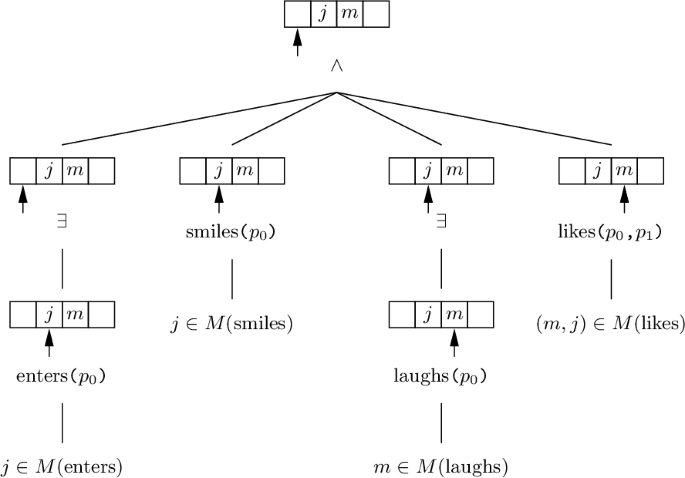
As an example of PLA in action, (8), can be rendered as (10).

• (10) $\exists x\text {enters}\mathtt ( x\mathtt ) \wedge \text {smiles}\mathtt ( p_{0}\mathtt ) \wedge \exists x\text {laughs}\mathtt ( x\mathtt ) \wedge \text {likes}\mathtt ( p_{0},p_{1}\mathtt )$

An evaluation of (10) is illustrated in (11), happening against the sequence of individuals $[m, j]$ and an assignment of $a$ to variable $x$. Conjunction in PLA is associative, so $(\phi \wedge \psi ) \wedge \chi \equiv \phi \wedge (\psi \wedge \chi )$, and to reflect this the illustration is left underspecified as to the order in which the instances of $\wedge$ apply.

• (11)

  

We can see that during the course of evaluation occurrences of $\wedge$ manage when frontmost positions of the sequence are kept in reserve for subsequent discourse. If positions are not reserved, they are either: (i) destined to be dropped to have their values entered into the assignment as existential binding values before a ‘test’ is encountered (either a predicate or negated formula), as demonstrated by the instances of $\exists x$; or (ii) serve as accessible old positions for pronouns, as demonstrated by the first $p_{0}$ instance and $p_{1}$ taking as antecedent the sequence value that serves as the binding value adopted by the first instance of $\exists x$, and the second instance of $p_{0}$ taking as antecedent the sequence value that serves as the binding value adopted by the second $\exists x$.

The binding value for an existential quantification comes from the sequence $\hat{\sigma }$. Pronouns likewise take their antecedent from $\hat{\sigma }$. Since $\hat{\sigma }$ is an open environment parameter of evaluation, this gives (10) the same interpretation as the predicate logic formula (12).

• (12) $\text {enters}\mathtt ( x_{1}\mathtt ) \wedge \text {smiles}\mathtt ( x_{1}\mathtt ) \wedge \text {laughs}\mathtt ( x_{2}\mathtt ) \wedge \text {likes}\mathtt ( x_{2},x_{1}\mathtt )$

This accords with the use of predicate logic in Cresswell (2002) to encode discourse while maintaining separable encodings for constituent sentences, e.g., (8) can be captured along the lines of (13).

• (13) $\exists x(x = x_{1} \wedge \text {enters}\mathtt ( x\mathtt ) ) \wedge \text {smiles}\mathtt ( x_{1}\mathtt ) \wedge \exists x(x = x_{2} \wedge \text {laughs}\mathtt ( x\mathtt ) ) \wedge \text {likes}\mathtt ( x_{2},x_{1}\mathtt )$

Furthermore, Cresswell suggests that what we are seeing as an essentially variable use of indefinites is reflected in English by the word “namely”, e.g., it is possible to say (14).

• (14) Someone, namely John, enters. He smiles. Someone, namely Mary, laughs.

  She likes him.

With the illustration of (11) we also see that what is the antecedent of a pronoun in PLA is not necessarily determined by the same index. Rather the antecedent of a pronoun must be calculated by taking into account the number of occurrences of existentials in intervening conjuncts. This seems appropriate for characterising pronouns. Pronouns do not have grammatically fixed antecedents and must instead have their antecedent resolved, that is, chosen from potentially a number of accessible antecedents. The index provides notation to indicate a specific choice of antecedent. Moreover, under the assumption that a lower integer is in some sense easier to allocate than a higher integer, pronouns are seen to favour closer (more salient) antecedents.

We are now in a position to consider PLA renderings of the examples in Sect. 1. Reading (3a) of (2) can be captured with the PLA formula (15a) that has bracketing conforming to (4a), while reading (3b) is captured by (15b) with bracketing that conforms to (4b).

• (15)

  • a. $\exists x(\text {collector}\mathtt ( x\mathtt ) \wedge \lnot \text {buy}\mathtt ( x\mathtt ) ) \wedge \text {influenced}\mathtt ( p_{0}\mathtt )$

  • b. $\exists x(\text {collector}\mathtt ( x\mathtt ) \wedge \lnot (\text {buy}\mathtt ( x\mathtt ) \wedge \text {influenced}\mathtt ( x\mathtt ) ))$

Due to the bracketing that makes the dependency with the pronoun a coordinating binding dependency in (15a) and a subordinating binding dependency in (15b) the encoding of the pronoun cannot be captured in a consistent manner: a dependency with the configuration of (1a) requires a PLA pronoun, while configuration (1b) necessitates a PLA variable.

Considering (5), the binding of the reflexive pronoun is captured with a PLA variable as in (16), while the covaluation data (6) necessitates a PLA pronoun as in (17).

• (16) $\exists x(\text {John}\mathtt ( x\mathtt ) \wedge \text {voted}\_\text {for}\mathtt ( x,x\mathtt ) )$

• (17) $\exists x(\text {John}\mathtt ( x\mathtt ) \wedge \text {voted}\_\text {for}\mathtt ( x,p_{1}\mathtt ) )$

Encodings (16) and (17) are appropriate for distinguishing covaluation from binding. PLA pronoun binding is essentially an ad-hoc dependency, with the actual dependency that obtains fixed with the allocation of an index for the pronoun—a change of index would allow a different antecedent. In contrast, the binding of a variable is determined solely by the scope under which the variable falls. This is appropriate for capturing dependencies that could not be otherwise, which holds for reflexive binding, but also for other clause internal dependencies, e.g., connecting subject and object arguments to the verb.

However the distinction between binding and covaluation achieved with (16) and (17) breaks down when we consider providing a PLA encoding for the covaluation reading of (7). Arising as the consequence of a subordinating configuration, the covaluation reading of (7) requires the pronoun to be coded with a PLA variable, as in (18).

• (18) $\lnot \exists x(\text {candidate}\mathtt ( x\mathtt ) \wedge \lnot (\text {surprised}\mathtt ( x\mathtt ) \wedge \lnot \exists y(\text {voted}\_\text {for}\mathtt ( y,x\mathtt ) \wedge \lnot y = x)))$

3 Only a Pronoun Mechanism

Context is structured with PLA as a sequence that is not changed but which can be extended with insertions from instances of negation that are subsequently lost on exit from the scope of the negation, resulting in DRT-like accessibility effects (see e.g., Kamp and Reyle 1993). Dynamism emerges from an advancing through the given context as managed by instances of $\wedge$, or to put this another way, the unveiling of previously inaccessible portions of context. The current position reached comes from a division between sequence values in active use and sequence values not in active use. Values in active use are either values that will be used as the values for quantifications in the current conjunct, in which case they are dropped from the sequence machinery and imported into the variable binding machinery, or else are values accessible to pronouns, in which case they will have been used as the values for quantifications in prior conjuncts. Values not in active use are held back to serve as values for the quantifications of subsequent conjuncts.

We might imagine other ways of keeping track on where we are in a structured context. In this section we consider a system with a “pointer” to mark the location reached in a linearly structured context which we can take to be an infinite sequence. Having infinite sequences removes the possibility of undefinedness, but the system would operate the same over finite sequences with sufficient sequence values.

Definition 2 (Pointer Semantics satisfaction and truth).

Suppose a first-order model $M$ with domain of individuals $D$. We will use $\hat{\sigma }[k..m]$ for finite sequence $(\hat{\sigma }_{k},\ldots ,\hat{\sigma }_{m})$, $\hat{\sigma }[k..\omega ]$ for the infinite sequence $(\hat{\sigma }_{k},\ldots )$, and $\hat{\sigma }[-\omega ..k]$ for the infinite sequence $(\ldots ,\hat{\sigma }_{k})$. We will write $\hat{\sigma }$ for $\hat{\sigma }[-\omega ..\omega ]$ and suppose individuals from $D$ are assigned to the positions of $\hat{\sigma }$. Satisfaction is given as follows:

• $M, \hat{\sigma } \models _{k} \exists \phi$ iff $M, \hat{\sigma } \models _{k+1} \phi$

• $M, \hat{\sigma } \models _{k} \phi \wedge \psi$ iff $M, \hat{\sigma } \models _{k} \phi$ and $M, \hat{\sigma } \models _{k+n(\phi )} \psi$

• $M, \hat{\sigma } \models _{k} \lnot \phi$ iff $M, \hat{\sigma }[-\omega ..k] \hat{\sigma }'[1..n(\phi )] \hat{\sigma }[k + 1..\omega ] \not \models _{k} \phi$     for all $\hat{\sigma }'[1..n(\phi )]$

• $M, \hat{\sigma } \models _{k} P(t_{1},\ldots ,t_{n})$ iff $([\![t_{1}]\!]_{\hat{\sigma }, k},\ldots ,[\![t_{n}]\!]_{\hat{\sigma }, k}) \in M(P)$

• $[\![p_{i}]\!]_{\hat{\sigma }, k} = \hat{\sigma }_{k-i}$

where $n(\phi )$ is a count of the binding operators $\exists$ in $\phi$ that are outside the scope of negation: $n(\exists \phi ) = n(\phi ) + 1$, $n(\phi \wedge \psi ) = n(\phi ) + n(\psi )$, $n(\lnot \phi ) = 0$, $n(P(t_{1},\ldots ,t_{n}))~=~0$.

A formula $\phi$ is true with respect $k$ and $\hat{\sigma }$ in $M$ iff there is a $\hat{\sigma }'[1..n(\phi )]$ such that $M, \hat{\sigma }[-\omega ..k] \hat{\sigma }'[1..n(\phi )] \hat{\sigma }[k + 1..\omega ] \models _{k} \phi$.

Binding operator $\exists \phi$ opens a fresh binding by advancing the pointer by one sequence value, which is thereafter accessible for pronouns inside $\phi$. With a conjunct $\phi \wedge \psi$, crossing to $\psi$ from $\phi$ advances the pointer by $n(\phi )$ sequence values, that is, by the number of instances of $\exists$ visible in $\phi$. This is demonstrated with a rendering of (8) as (19).

• (19) $\exists \text {enters}\mathtt ( p_{0}\mathtt ) \wedge \text {smiles}\mathtt ( p_{0}\mathtt ) \wedge \exists \text {laughs}\mathtt ( p_{0}\mathtt ) \wedge \text {likes}\mathtt ( p_{0},p_{1}\mathtt )$

Evaluation of (19) is illustrated in (20), with the order in which the three instances of $\wedge$ apply left underspecified, since conjunction is associative, as was the case with PLA. Also note how the evaluation of terminals ends exactly as with (11).

• (20)

  

Negation works as illustrated in (21) by inserting into the main sequence a sequence of values that serve as the positions to which the pointer is moved by existentials while inside the scope of negation, returning back to the main sequence outside the scope of negation.

• (21)

  

We are now in a position to apply the system of Pointer Semantics to the examples of Sect. 1. Reading (3a) of (2) follows from (22a) with bracketing conforming to (4a), while reading (3b) is captured by (22b) with bracketing that conforms to (4b).

• (22)

  • a. $\exists (\text {collector}\mathtt ( p_{0}\mathtt ) \wedge \lnot \text {buy}\mathtt ( p_{0}\mathtt ) ) \wedge \text {influenced}\mathtt ( p_{0}\mathtt )$

  • b. $\exists (\text {collector}\mathtt ( p_{0}\mathtt ) \wedge \lnot (\text {buy}\mathtt ( p_{0}\mathtt ) \wedge \text {influenced}\mathtt ( p_{0}\mathtt ) ))$

Reflexive binding in (5) is captured with (23), while covaluation readings for (6) and (7) are obtained with (24) and (25), respectively.

• (23) $\exists (\text {John}\mathtt ( p_{0}\mathtt ) \wedge \text {voted}\_\text {for}\mathtt ( p_{0},p_{0}\mathtt ) )$

• (24) $\exists (\text {John}\mathtt ( p_{0}\mathtt ) \wedge \text {voted}\_\text {for}\mathtt ( p_{0},p_{1}\mathtt ) )$

• (25) $\lnot \exists (\text {candidate}\mathtt ( p_{0}\mathtt ) \wedge \lnot (\text {surprised}\mathtt ( p_{0}\mathtt ) \wedge \lnot \exists (\text {voted}\_\text {for}\mathtt ( p_{0},p_{1}\mathtt ) \wedge \lnot p_{0}~{=}~p_{1})))$

The encodings of (22)–(25) successfully capture the uniform role of linking played by pronouns in both subordinating and coordinating configurations. However this uniformity is achieved at the expense of turning all operator-variable dependencies into PLA-like pronominal bindings, including internal clause relations, such as subject arguments binding verbal predicates. As was noted when looking at PLA, PLA pronouns capture the ad-hoc nature of pronominal linking, with the actual dependency that holds relying on a choice of index with respect to the presence of intervening (formula) material. This is inappropriate for capturing core clause internal links, which need to be grammatically enforced and essentially unalterable dependencies, but see van Eijck (2001) where a constrained system of pronoun management is developed in a dynamic setting. What we appear to need is a system that has both the option of pronominal linking and variable name linking with subordinating configurations.

4 Only Coordinating Binding Dependencies

In this section we look at Dynamic Predicate Logic with Exit operators (DPLE) as introduced by Vermeulen (1993, 2000), Hollenberg and Vermeulen (1996), with the exception that we adopt predicate logic notation for the purpose of comparison. The system itself extends the system of Dynamic Predicate Logic from Groenendijk and Stokhof (1991) with the distinctive feature of treating the scoping of variables by means of sequences. Each variable is assigned its own sequence by a sequence assignment. This allows the introduction of an Exit operator for terminating otherwise persistent dynamic scopes.

We will illustrate sequence assignments at work. The sequence value of an assignment to a variable is depicted directly above the variable as boxes on top of each other forming a stack. The uppermost box is the frontmost element of the sequence. Only sequences for variable of interest are represented. For example, (26) illustrates an assignment $g$ with $g(x) = [c, a]$ and $g(y) = [b]$.

• (26)

  

The DPLE system builds on a primitive relation pop on sequence assignments:

• $(g,h) \in {\small \mathtt {pop}}_{x}$ iff $h$ is just like $g$, except that $g(x) = {\small \mathtt [}(g(x))_{0}{\small \mathtt ]}$ @ $h(x)$.

There are actually two ways to interpret $(g,h) \in \mathtt{pop}_{x}$. Read from $g$ to $h$ the relation describes the popping of the frontmost sequence element that is assigned to $x$ by $g$. Read from $h$ to $g$ the relation describes the pushing of a new sequence value onto the front of the sequence that is assigned to $x$ by $h$. An example is illustrated in (27).

• (27)

  

Formulas are interpreted as relations on sequence assignments that change the before-state of a sequence assignment to an after-state in accordance with definition 3.

Definition 3 (DPLE satisfaction and truth).

Suppose a first-order model $M$ with domain of individuals $D$. Suppose $SA$ is the set of assignments from variables to sequences of individuals from $D$. Each formula $\phi$ is assigned to a relation $[\![\phi ]\!]_{M} \subseteq SA \times SA$ as follows:

• $(g,h) \in [\![\phi \wedge \psi ]\!]_{M}$ iff $\exists j: (g,j) \in [\![\phi ]\!]_{M}$ and $(j,h) \in [\![\psi ]\!]_{M}$

• $(g,h) \in [\![ \exists x ]\!]_{M}$ iff $(h,g) \in {\small \mathtt {pop}}_{x}$

• $(g,h) \in [\![ Exit_{x} ]\!]_{M}$ iff $(g,h) \in {\small \mathtt {pop}}_{x}$

• $(g,h) \in [\![x = y]\!]_{M}$ iff $g = h$ and $(g(x))_{0} = (g(y))_{0}$

• $(g,h) \in [\![ \text {P}\mathtt ( x_{1},\ldots ,x_{n}\mathtt ) ]\!]_{M}$ iff $g = h$ and $((g(x_{1}))_{0},\ldots ,(g(x_{n}))_{0}) \in M(\text {P})$

• $(g,h) \in [\![\lnot \phi ]\!]_{M}$ iff $g = h$ and $\lnot \exists j : (g, j) \in [\![\phi ]\!]_{M}$

A formula $\phi$ is true with respect to $g$ in $M$ iff there is a $h$ such that $(g, h) \in [\![\phi ]\!]_{M}$.

From definition 3, we see how the after-state of a formula is the before-state of the next conjoined formula. Existential quantification is captured as the pushing of a random value onto the front of the $x$-sequence of the input assignment, while the Exit operator is realised as the popping of the frontmost value of the $x$-sequence. Predicate formulas correspond to tests on the frontmost values of variable sequences. The implementation of negation follows Dynamic Predicate Logic in possibly changing the assignment only internally to the scope of negation to act overall as a static test.

The DPLE system can be employed to provide a rendering of (8) as in (28).

• (28) $\exists x \wedge \text {enters}\mathtt ( x\mathtt ) \wedge \text {smiles}\mathtt ( x\mathtt ) \wedge \exists y \wedge \text {laughs}\mathtt ( y\mathtt ) \wedge \text {likes}\mathtt ( x,y\mathtt )$

Reading (3a) of (2) obtains with the formula (29a) with bracketing that conforms to (4a), while reading (3b) is captured by (29b) with bracketing that conforms to (4b).

• (29)

  • a. $\exists x \wedge \text {collector}\mathtt ( x\mathtt ) \wedge \lnot \text {buy}\mathtt ( x\mathtt ) \wedge \text {influenced}\mathtt ( x\mathtt )$

  • b. $\exists x \wedge \text {collector}\mathtt ( x\mathtt ) \wedge \lnot (\text {buy}\mathtt ( x\mathtt ) \wedge \text {influenced}\mathtt ( x\mathtt ) )$

Reflexive binding in (5) is captured with (30), while covaluation readings for (6) and (7) are obtained with (31) and (32), respectively.

• (30) $\exists x \wedge \text {John}\mathtt ( x\mathtt ) \wedge \text {voted}\_\text {for}\mathtt ( x,x\mathtt )$

• (31) $\exists x \wedge \text {John}\mathtt ( x\mathtt ) \wedge \text {voted}\_\text {for}\mathtt ( x,y\mathtt )$

• (32) $\lnot (\exists x \wedge \text {candidate}\mathtt ( x\mathtt ) \wedge \lnot (\text {surprised}\mathtt ( x\mathtt ) \wedge \lnot (\exists y \wedge \text {voted}\_\text {for}\mathtt ( y,x\mathtt ) \wedge \lnot y = x)))$

However the encodings of (28)–(32) are essentially what we might have expected to give had we been employing the system of Dynamic Predicate Logic, because there is no use made of the one feature that is unique to DPLE, namely the Exit operator.

As a more interesting application of DPLE consider (33). This acts to move the frontmost element of the $x$-sequence to the front of the $y$-sequence, where $x \ne y$.

• (33) $\mathtt{{move}}_{x, y} \equiv \exists y \wedge x = y \wedge Exit_{x}$

We can give (34) as an illustration of how (33) works.

• (34)

  

From (34) we see how $\exists y$ changes an input assignment to a new assignment where what was the original content of the $y$-sequence is stored ‘under’ a new frontmost element. For the next instruction to succeed the new frontmost element of the $y$-sequence must be $a$, else $x = y$ fails. Consequently, $\exists y \wedge x = y$ has a unique output. Then $Exit_{x}$ applies to remove the frontmost element of the $x$-sequence to give the final output.

To illustrate an application for move of (33) let us define operations $\bullet$ and $\square$, where utilisation of the specific variables $sbj$, $obj$ and $p$ is rigidly fixed by the definitions.

• (35) $\bullet \equiv \mathtt{{move}}_{sbj, p}$

  $\square \equiv \mathtt{{move}}_{obj, p} \wedge \bullet$

Let us also employ the convention in (36) to bring about formula iteration.

• (36) $R^{0} \equiv \top$

  $R^{n} \equiv R^{n - 1}\wedge R$

We will now aim to mimic the contribution of some English words and phrases with DPLE expressions. In (37) we define the contribution of several subject noun phrases that create sbj bindings, noting that sbj variable names are rigidly specified as parts of the encodings.

• (37) ${\small \mathtt {Someone}} \equiv \exists sbj$

  ${\small \mathtt {A}}\_\mathtt{{collector}} \equiv \exists sbj \wedge \text {collector}\mathtt ( sbj\mathtt )$

  ${\small \mathtt {John}} \equiv \exists sbj \wedge \text {John}\mathtt ( sbj\mathtt )$

  ${\small \mathtt {every}}\_\mathtt{{candidate}}~\phi \equiv \lnot (\exists sbj \wedge \text {candidate}\mathtt ( sbj\mathtt ) \wedge \lnot \phi )$

In (38) we aim to capture the contribution of both subject and object pronouns that have an open $i$ parameter to take an index value, as well as a subject pronoun that is accompanied by only and also a reflexive pronoun. The reflexive pronoun has no index but is rather rigidly fixed to create an $obj$ binding that is linked to the open $sbj$ binding.

• (38) ${\small \mathtt {she}}_{i}, {\small \mathtt {he}}_{i} \equiv \exists sbj \wedge ({\small \mathtt {move}}_{p, r})^{i} \wedge sbj = p \wedge ({\small \mathtt {move}}_{r, p})^{i}$

  ${\small \mathtt {her}}_{i}, {\small \mathtt {him}}_{i} \equiv \exists obj \wedge obj = p \wedge ({\small \mathtt {move}}_{p, r})^{i} \wedge ({\small \mathtt {move}}_{r, p})^{i}$

  ${\small \mathtt {only}}\_\mathtt{{he}}_{i}~\phi \equiv \lnot (\exists sbj \wedge \phi \wedge \lnot (({\small \mathtt { move}}_{p, r})^{i} \wedge sbj = p))$

  ${\small \mathtt {herself}}, {\small \mathtt {himself}} \equiv \exists obj \wedge obj = sbj$

Finally we provide DPLE encodings for verbs in (39), again noting that the variable instances are rigidly specified.

• (39) ${\small \mathtt {enters}} \equiv \text {enters}\mathtt ( sbj\mathtt ) , {\small \mathtt {smiles}} \equiv \text {smiles}\mathtt ( sbj\mathtt ) , {\small \mathtt {laughs}} \equiv \text {laughs}\mathtt ( sbj\mathtt ) ,$

  ${\small \mathtt {likes}} \equiv \text {likes}\mathtt ( sbj,obj\mathtt ) , {\small \mathtt {buy}} \equiv \text {buy}\mathtt ( sbj\mathtt ) , {\small \mathtt {was}}\_\mathtt{{influenced}} \equiv \text {influenced}\mathtt ( sbj\mathtt ) ,$

  ${\small \mathtt {voted}}\_\mathtt{{for}} \equiv \text {buy}\mathtt ( sbj\mathtt ) , {\small \mathtt {is}}\_\mathtt{{surprised}} \equiv \text {surprised}\mathtt ( sbj\mathtt )$

We are now in a position to consider (40) as a rendering of (8).

• (40) ${\small \mathtt {Someone}} \wedge {\small \mathtt {enters}} \wedge \bullet \wedge {\small \mathtt {he}}_{0} \wedge {\small \mathtt {smiles}} \wedge \bullet \wedge {\small \mathtt {Someone}} \wedge {\small \mathtt {laughs}} \wedge \bullet \wedge$

  ${\small \mathtt {she}}_{0} \wedge {\small \mathtt { him}}_{1} \wedge {\small \mathtt {likes}} \wedge \square$

In (41) an illustration is given of the changes that arise to a sequence assignment when (40) is evaluated, resulting in terminals that end exactly as with (11) and (20).

• (41)

  

We can also capture reading (3a) of (2) with (42a), while reading (3b) follows from (42b).

• (42)

  • (a.) ${\small \mathtt {A}}\_\mathtt{{collector}} \wedge \lnot {\small \mathtt {buy}} \wedge \bullet \wedge {\small \mathtt {she}}_{0} \wedge {\small \mathtt {was}}\_\mathtt{{influenced}} \wedge \bullet$

  • (b.) ${\small \mathtt {A}}\_\mathtt{{collector}} \wedge \lnot ({\small \mathtt {buy}} \wedge \bullet \wedge {\small \mathtt {she}}_{0} \wedge {\small \mathtt {was}}\_\mathtt{{influenced}}) \wedge \bullet$

Reflexive binding in (5) is captured with (43), while covaluation readings for (6) and (7) are obtained with (44) and (45), respectively.

• (43) ${\small \mathtt {John}} \wedge {\small \mathtt {himself}} \wedge {\small \mathtt {voted}}\_\mathtt{{for}} \wedge \square$

• (44) ${\small \mathtt {John}} \wedge {\small \mathtt {him}}_{0} \wedge {\small \mathtt {voted}}\_\mathtt{{for}} \wedge \square$

• (45) ${\small \mathtt {every}}\_{\small \mathtt {candidate}}~({\small \mathtt {is}}\_{\small \mathtt {surprised}} \wedge \bullet \wedge {\small \mathtt {only}}\_\mathtt{{he}}_{0}~({\small \mathtt {him}}_{0} \wedge {\small \mathtt {voted}}\_{\small \mathtt {for}}))$

Examples (40) and (42)–(45) illustrate how it is possible to make bindings with DPLE uniform and principled with the dependency management that the Exit operator makes possible. However this comes at the cost of having to stipulate management instructions. Worse still, relevant management instructions are dependent on what has gone on before, with there being different ways to terminate a sentence, notably, $\square$, $\bullet$ or no operation, depending on whether the sentence contains an object, only a subject, or falls under the scope of negation. To sum up, DPLE facilitates achieving uniform bindings. What we now require is a way to automate the management of open dependencies. This we aim to achieve with the system of the next section.

5 Pronominal and Variable Binding Again

In this section we illustrate a system with options for pronominal and variable name binding in subordinating contexts, and the option of pronominal binding for coordinating contexts.

One way to achieve such a system would be to place the machinery of predicate logic alongside Pointer Semantics of Sect. 3. While feasible, the resulting system would have two binding options—pronominal and variable binding—simultaneously available for subordinating dependencies. In a natural language like English the distinct binding options of reflexive binding and pronominal binding have a complementary distribution.

What we aim for instead in this section is to present a system that has quantification to open a variable binding that will serve as the mechanism for establishing grammatically determined dependencies such as linking subject and object arguments to the main predicate as well as reflexive binding, and for this to be subsequently handed over to a binding that is available to the pronominal machinery, either as part of a coordinating dependency or as part of a sufficiently embedded subordinating dependency. This will be accomplished with some of the dynamic control DPLE allowed over sequence assignments.

First we introduce the operations of cons and snoc:

• cons adds an element to the front of a sequence: cons $y$ $\hat{x} = {\small \mathtt [}y{\small \mathtt ]}$ @ $\hat{x}$.

• snoc adds an element to the end of a sequence: snoc $y$ $\hat{x} = \hat{x}$ @ ${\small \mathtt [}y{\small \mathtt ]}$.

We now define shift( $op$ ) on pairs of assignments $(g, h)$ to move from $g$ to $h$ or vice versa. For shift( $op$ ) the operation $op$ needs to be specified, with suitable candidates being cons and snoc to give shift(cons) and shift(snoc).

• $(g,h) \in {\small \mathtt {shift(}}op{\small \mathtt )}_{x,y}$ iff $\exists k:$ $(h, k) \in {\small \mathtt {pop}}_{y}$ and $k$ is just like $g$, except that $g(x) = op((h(y))_{0}{\small \mathtt ,}k(x))$.

We will also use an iteration convention for relations on sequence assignments, e.g., implemented as in (36).

Reading from $g$ to $h$, $(g,h) \in \mathtt{{shift(cons)}}_{x, y}$ moves the frontmost scope of the $x$ sequence to the front of the $y$ sequence. Examples are given in (46): (46a) illustrates a single action of shift(cons); (46b) illustrates how iterated shift(cons) can move a sequence of scopes to the front of another sequence with the original ordering of scopes reversed.

• (46)

  

Reading from $g$ to $h$, $(g,h) \in \mathtt{{shift(snoc)}}_{x, y}$ moves the endmost scope of the $x$ sequence to the front of the $y$ sequence. Examples are given in (47): (47a) illustrates a single action of shift(snoc); (47b) illustrates how iterated shift(snoc) can move a sequence of scopes to the front of another sequence with the original ordering of scopes intact.

• (47)

  

Having iterable relations shift(cons) and shift(snoc) in addition to pop from Sect. 4, we introduce a minimal version of Scope Control Theory (SCT) from Butler (2010).

Definition 4 (Minimal Scope Control Theory satisfaction and truth).

Formulas are evaluated with respect to a first-order model $M = (D, I)$ and sequence assignment $g \in SA$, where $SA$ is the set of assignments from variables to sequences of individuals from $D$. First, we define term evaluation:

• $g(v_{n}) = d$ if $\exists h : (h, g) \in {\small \mathtt {pop}}_{v}^{i}$ and $d = \uparrow \!\! (h(v))$, else undefined.

Next, we define formula evaluation:

• $M, g \models \exists x \phi$ iff $\exists h : (g,h) \in {\small \mathtt {shift(cons)}}_{e, x}$ and $M, h \models \phi$

• $M, g \models \rceil x \phi$ iff $\exists h : (g,h) \in {\small \mathtt {shift(cons)}}_{x, p}$ and $M, h \models \phi$

• $M, g \models \phi \wedge \psi$ iff $\exists h : ((g,h) \in {\small \mathtt {pop}}_{e}^{n(\psi )}$ and $M, h \models \phi )$ and $\exists h ((g,h) \in {\small \mathtt {shift(snoc)}}_{e, p}^{n(\phi )}$ and $M, h \models \psi )$

• $M, g \models \lnot \phi$ iff $\lnot \exists h : (h,g) \in {\small \mathtt {pop}}_{e}^{n(\phi )}$ and $M, h \models \phi$

• $M, g \models P(t_{1}, \ldots , t_{n})$ iff $(g(t_{1}), \ldots , g(t_{n})) \in I(P)$

where $n(\phi )$ is a count of existentials in $\phi$ that are outside the scope of negation: $n(\exists x \phi ) = n(\phi ) + 1$, $n(\rceil x \phi ) = n(\phi )$, $n(\phi \wedge \psi ) = n(\phi ) + n(\psi )$, $n(\lnot \phi ) = 0$, $n(\text {P}\mathtt ( t_{1},\ldots ,t_{n}\mathtt ) ) = 0$.

A formula $\phi$ is true with respect to $g$ in $M$ iff there is a $h \in SA$ such that $(h, g) \in \mathtt{pop}_{e}^{n(\psi )}$ and $M, h \models \phi$.

A term has form $v_{n}$ in a predicate formula $\text {P}\mathtt ( \ldots v_{n}\ldots \mathtt )$, and denotes the $n~+~1$ element of the $v$-sequence. In practice, indices different from $0$ appear rarely. Nevertheless, they can appear. We will assume the convention that the index 0 can be omitted to keep the language to a conservative extension of traditional predicate logic notation.

The existential quantifier is defined to trigger an instance of shift(cons) that relocates the frontmost sequence element of the $e$-sequence to the $x$-sequence, where $e$ is a privileged name and $x$ is determined by the quantification instance. Similarly $\rceil x$ serves to relocate with shift(cons) an assigned sequence value, only relocating the frontmost value of the $x$-sequence, where $x$ is determined by the given instance of $\rceil x$, to become the frontmost sequence value that is assigned to the privileged $p$ variable.

Conjunction also acts to modify the content of what is assigned to the privileged variables of $e$ and $p$. Before evaluation of the first conjunct can proceed, the $e$-sequence has $n(\psi )$ values popped. Before evaluation of the second conjunct can proceed, there is the relocation with shift(snoc) of $n(\phi )$ values from the end of the sequence assigned to $e$ to the front of the sequence that is assigned to $p$. Evaluation of $\lnot \phi$ involves showing there is no way to extend the sequence assigned to the privileged $e$ variable by $n(\phi )$ sequence values and have $\phi$ hold true.

Having now introduced Minimal SCT we can demonstrate the system with a rendering of (8) as in (48), which is syntactically identical to the PLA rendering of (10).

• (48) $\exists x\text {enters}\mathtt ( x\mathtt ) \wedge \text {smiles}\mathtt ( p_{0}\mathtt ) \wedge \exists x\text {laughs}\mathtt ( x\mathtt ) \wedge \text {likes}\mathtt ( p_{0},p_{1}\mathtt )$

An evaluation of (48) is illustrated in (49), with the ordering of the three instances of $\wedge$ left underspecified since conjunction is once again associative, and happening against a sequence assignment with an initial state in which $e$ is assigned the sequence $[m, j]$ while other variables are assigned the empty sequence. As the evaluation proceeds this assignment is modified, so that the terminals end exactly as with (11), (20) and (41).

• (49)

  

Reading (3a) of (2) is captured with the formula (50a) with bracketing that conforms to (4a), while reading (3b) is captured by (50b) with bracketing that conforms to (4b). It is with the rendering of (50b) that we see the first deviation from what was possible with PLA. Notably (50b) employs $\rceil x$ with the consequence that the pronoun can be rendered as $p_{0}$ and so uniformity is achieved with the treatment of the pronoun in (50a).

• (50)

  • a. $\exists x(\text {collector}\mathtt ( x\mathtt ) \wedge \lnot \text {buy}\mathtt ( x\mathtt ) ) \wedge \text {influenced}\mathtt ( p_{0}\mathtt )$

  • b. $\exists x(\text {collector}\mathtt ( x\mathtt ) \wedge \lnot (\text {buy}\mathtt ( x\mathtt ) \wedge \rceil x \text {influenced}\mathtt ( p_{0}\mathtt ) ))$

Reflexive binding in (5) is captured with (51), while covaluation readings for (6) and (7) are obtained with (52) and (53), respectively. Again this illustrates the consistent use of variables named $p$ (akin to PLA-like pronouns) to capture English pronouns, while other variables capture clause internal linking and reflexive binding.

• (51) $\exists x(\text {John}\mathtt ( x\mathtt ) \wedge \text {voted}\_\text {for}\mathtt ( x\mathtt , x\mathtt ) )$

• (52) $\exists x(\text {John}\mathtt ( x\mathtt ) \wedge \text {voted}\_\text {for}\mathtt ( x\mathtt , p_{0}\mathtt ) )$

• (53) $\lnot \exists x(\text {candidate}\mathtt ( x\mathtt ) \wedge \lnot (\text {surprised}\mathtt ( x\mathtt ) \wedge \rceil x \lnot \exists y(\text {voted}\_\text {for}\mathtt ( y\mathtt , p_{0}\mathtt ) \wedge \lnot y~{=}~p_{0})))$

With the management of dependencies that occurs with conjunction and the $\rceil$-operator it is possible to establish a more direct correspondence with a natural language like English. For example, following what was possible in (37) with DPLE, we define the contribution of several subject noun phrases in (54) with rigidly prescribed bindings.

• (54) ${\small \mathtt {Someone}}~\phi \equiv \exists sbj \phi$

  ${\small \mathtt {A}}\_\mathtt{{collector}}~\phi \equiv \exists sbj(\text {collector}\mathtt ( sbj\mathtt ) \wedge \phi )$

  ${\small \mathtt {John}}~\phi \equiv \exists sbj(\text {John}\mathtt ( sbj\mathtt ) \wedge \phi )$

  ${\small \mathtt {every}}\_\mathtt{{candidate}}~\phi \equiv \lnot \exists sbj(\text {candidate}\mathtt ( sbj\mathtt ) \wedge \lnot \phi )$

In (55) we capture subject and object pronouns, as well as a subject pronoun accompanied by only and also a reflexive pronoun.

• (55) ${\small \mathtt {she}}_{i}, {\small \mathtt {he}}_{i}~\phi \equiv \exists sbj(sbj = p_{i} \wedge \phi )$

  ${\small \mathtt {her}}ensuremath{_{i}}, {\small \mathtt {him}}_{i}~\phi \equiv \exists obj(obj = p_{i} \wedge \phi )$

  ${\small \mathtt {only}}\_\mathtt{{he}}_{i}~\phi \equiv \lnot \exists sbj(\phi \wedge \lnot sbj = p_{i})$

  ${\small \mathtt {herself}}, {\small \mathtt {himself}}~\phi \equiv \exists obj(obj = sbj \wedge \phi )$

Having (54)–(55), and adopting the codings of verbs in (39) without change, we are in a position to render (8) as (56), The notable advantage over the DPLE version of (40) is that there is no longer a need for the explicit management instructions of $\bullet$ and $\square$.

• (56) ${\small \mathtt {Someone}}~{\small \mathtt {enters}} \wedge {\small \mathtt {he}}_{0}~{\small \mathtt {smiles}} \wedge {\small \mathtt {Someone}}~{\small \mathtt {laughs}} \wedge {\small \mathtt {she}}_{0}~({\small \mathtt {him}}_{1} {\small \mathtt {likes}})$

Reading (3a) of (2) is captured with (57a), while reading (3b) follows from (57b).

• (57)

  • a. ${\small \mathtt {A}}\_\mathtt{{collector}}~\lnot {\small \mathtt {buy}} \wedge {\small \mathtt {she}}_{0}~{\small \mathtt {was}}\_\mathtt{{influenced}}$

  • b. ${\small \mathtt {A}}\_\mathtt{{collector}}~\lnot ({\small \mathtt {buy}} \wedge \rceil sbj ({\small \mathtt {she}}_{0}~{\small \mathtt {was}}\_\mathtt{{influenced}}))$

Reflexive binding in (5) is captured with (58), while covaluation readings for (6) and (7) are obtained with (59) and (60), respectively.

• (58) ${\small \mathtt {John}}~({\small \mathtt {himself}}~{\small \mathtt {voted}}\_\mathtt{{for}})$

• (59) ${\small \mathtt {John}}~({\small \mathtt {him}}_{0}~{\small \mathtt {voted}}\_\mathtt{{for}})$

• (60) ${\small \mathtt {every}}\_\mathtt{{candidate}}~({\small \mathtt {is}}\_\mathtt{{surprised}} \wedge \rceil sbj ({\small \mathtt {only}}\_\mathtt{{he}}_{0}~({\small \mathtt {him}}_{0}~{\small \mathtt {voted}}\_\mathtt{{for}})))$

An apparent weakness that remains with the encodings of (57b) and (60) is that the management of $\rceil sbj$ must be stipulated. What we require is a trigger to motivate the hand-over from a non-$p$(ronominal) binding to a $p$ binding. We might suppose such hand overs come about whenever the non-$p$ binding is set to be reused. So in the examples of (57b) and (60) the fact that a new clause is entered which itself contains a subject argument opening a $sbj$ binding is reason enough for the occurrence of $\rceil sbj$.

Extending this rational we should expect that when there is no subject in an embedded clause there will be no corresponding $\rceil sbj$, e.g., with the consequence that a $sbj$ dependency can be maintained across a clause boundary, as holds for the control dependency in (61).

• (61) John needed to go.

Interestingly a control predicate may take as complement an embedded clause that contains a main predicate that is unable to receive a subject binding, but only provided there is the presence of expletive it, as the contrast between (62a) and (62b) demonstrates.

• (62)

  • a. John needed it to rain.

  • b. *John needed to rain.

Supposing expletive it to contribute $\rceil sbj$ removes the subject binding inherited from the control verb before rain is encountered.

Finally we should note that for the current approach to scale, e.g., to handle passivisation, a more sophisticated interaction with syntax is required to implement how binding names are obtained, which is left for future work.

6 Summary

This chapter began with the observation that in English properties for coordinating dependencies also held for sufficiently deeply embedded subordinating dependencies. This was taken to suggest that the two dependency types arise with the same mechanism, and the purpose of this chapter has been to explore formal ways to implement such a mechanism. This chapter has ended with a system that preserves classical variable name binding, which captures well the more restricted role of clause internal argument linking and reflexive binding in natural language, and have a subsequent hand-over to a pronominal machinery in subordinating contexts with sufficient embedding, which captures well the ad-hoc nature of pronominal binding. The set up of the system was such that the same pronominal machinery carried over as the means to establish dependencies across coordinating contexts. With its management of dependencies the system was demonstrated to reduce the distance between natural language form and its realisation as a formula for interpretation.

References

Büring, D. (2005). Bound to bind. Linguistic Inquiry, 36(2), 259–274.
Butler, A. (2010). The semantics of grammatical dependencies, vol. 23 of current research in the semantics/pragmatics interface. Bingley: Emerald.
Cresswell, M. J. (2002). Static semantics for dynamic discourse. Linguistics and Philosophy, 25, 545–571.
Dekker, Paul. (2002). Meaning and use of indefinite expressions. Journal of Logic, Language and Information, 11, 141–194.
Groenendijk, Jeroen, & Stokhof, Martin. (1991). Dynamic predicate logic. Linguistics and Philosophy, 14(1), 39–100.
Heim, I. (1993). Anaphora and semantic interpretation: A reinterpretation of Reinhart’s approach. Technical report SfS-Report-07-93, University of Tübingen.
Hollenberg, M., & Vermeulen, C. F. M. (1996). Counting variables in a dynamic setting. Journal of Logic and Computation, 6, 725–744.
Kamp, H., & Reyle, U. (1993). From discourse to logic: Introduction to model-theoretic semantics of natural language, formal logic and discourse representation theory. Dordrecht: Kluwer.
Reinhart, T. (2000). Strategies of anaphora resolution. In H. Bennis, M. Everaert, & E. Reuland (Eds.), Interface strategies (pp. 295–325). Amsterdam: Royal Academy of Arts and Sciences.
van Eijck, J. (2001). Incremental dynamics. Journal of Logic, Language and Information, 10, 319–351.
Vermeulen, C. F. M. (1993). Sequence semantics for dynamic predicate logic. Journal of Logic, Language and Information, 2, 217–254.
Vermeulen, C. F. M. (2000). Variables as stacks: A case study in dynamic model theory. Journal of Logic, Language and Information, 9, 143–167.
Acknowledgments
This research has been supported by the Japan Science and Technology Agency PRESTO program (Synthesis of Knowledge for Information Oriented Society). I would like to thank the three anonymous reviewers for their extremely helpful comments that prompted considerable improvements to the chapter.
Author information
Authors and Affiliations
Corresponding author
Editor information
Editors and Affiliations
Rights and permissions
Copyright information
© 2014 Springer Science+Business Media Dordrecht
About this chapter
Cite this chapter
Butler, A. (2014). Coordinating and Subordinating Binding Dependencies. In: McCready, E., Yabushita, K., Yoshimoto, K. (eds) Formal Approaches to Semantics and Pragmatics. Studies in Linguistics and Philosophy, vol 95. Springer, Dordrecht. https://doi.org/10.1007/978-94-017-8813-7_4
Download citation
DOI: https://doi.org/10.1007/978-94-017-8813-7_4
Publisher Name: Springer, Dordrecht
Print ISBN: 978-94-017-8812-0
Online ISBN: 978-94-017-8813-7
eBook Packages: Humanities, Social Sciences and LawSocial Sciences (R0)