Numerical Analysis of Nonholonomic Elastoplastic Frames by Mathematical Programming

Abstract

The strength as well as the ductility of a structure may be estimated by performing an elastoplastic analysis. In such an analysis structural loading is incrementally applied through a proportional loading factor in accordance to a predefined loading pattern. During this process we have continuous plasticizations of various parts of the structure. For a more accurate description of the physical process, possible deplasticizations should also be taken into account. Thus a nonholonomic material behavior should be followed. In this work such an analysis is performed in an efficient way. The basis of the approach is the formulation of the incremental problem as a convex parametric quadratic programming (PQP) problem between two successive plastic hinges. The solution of this problem is done by assuming a fictitious load factor which establishes a search direction for the next plasticization. The true load factor is established when the plastic hinge that is closest to open really opens. An example of application, which serves as benchmark, is also included.

These keywords were added by machine and not by the authors. This process is experimental and the keywords may be updated as the learning algorithm improves.

1 Introduction

The capacity of a structure beyond its elastic limits may be estimated by performing a step-by-step elastoplastic analysis. During this process the loading is applied sequentially with consecutive parts of the structure being plasticized. Between two plasticizations an elastic analysis is performed. Thus a series of elastic analyses is carried out before reaching either a limit load state or a predefined load state. In this way, one may have a good estimate of the structure’s strength as well as of its ductility. The above described procedure is called holonomic plasticity.

A more realistic material behavior is to take into account any local unloading (plastic unstressing) in the course of the analysis. This approach, which is much more involved computationally, is called nonholonomic plasticity.

Maier [1] was the first to show that mathematical programming (MP) and especially parametric quadratic programming (PQP) provides a unified formalism for the problem of elastoplastic analysis with the load factor being the parameter of the program. In this work holonomic plasticity has been addressed. The alternative formulation as a parametric complementarity problem (PLCP) has also been given by Maier [2]. The framework for this problem is linear programming (LP) with the Simplex method employed for its solution (de Donato and Maier [3]). Smith [4] extended this approach to nonholonomic plasticity proposing a numerical solution based on the Simplex method that restricts the variables that enter the basis. The methodology was applied to a simple frame. In an attempt to produce a PLCP based general purpose computer program for nonholonomic plasticity Franchi and Cohn [5] and Kaneko [6] proposed a rather involved algorithm. PLCP based solutions of problems with a softening material behavior have also appeared recently (Tangaramvong and Tin-Loi [7, 8]).

Besides the compact MP formulation of an elastoplastic problem, all the above PLCP based solutions generally involve a large number of variables and constraints (Tin-Loi and Wong [9]). At the same time computer implementation of these algorithms is quite difficult. Thus an alternative approach, the direct stiffness method has almost exclusively been used. This is based on the displacement method and whenever a plasticization occurs, an elastic prediction—plastic correction takes place by re-formulating and re-decomposing the stiffness matrix. Re-formulation and re-decomposition, must also take place if nonholonomicity is considered. These two tasks increase the computational time quite considerably.

The present work presents a methodology that was proposed by Spiliopoulos and Patsios [10]. The main ingredient of the procedure is to cast the problem in the form of an incremental PQP and solve it directly in this form. A numerical strategy was developed that employs a fictitious load factor and solves the resulting QP program by standard algorithms (e.g. Goldfarb and Idnani [11]). The solution of the fictitious program will automatically detect a possible unstressing and, at the same time, it establishes a solution direction which searches for the formation of the next plastic hinge which is closest to open. When it opens, the load factor receives its true value.

The approach appears to be numerically stable and very fast. Although it may be formulated either with respect to a displacement based or a force based MP, the force based one is preferred, due to the less number of unknowns and to the accurate way that equilibrium is expressed through this method. An approach (Spiliopoulos [12]) may be used to automatically establish this equilibrium both with respect to the hyperstatic forces and the applied loading.

2 Problem Formulation

Let a frame, whose material is elastic-perfectly plastic, be subjected to a loading pattern which changes in a proportional way:

$$ \mathbf{P} = \mathbf{P}_{in} + \gamma\cdot\mathbf{r}_{P} $$

(1)

where bold letters represent vectors and matrices, P _in represents an initial load state, γ is a proportional load factor and r _p is the unit vector along the direction of the loading pattern (Fig. 1). This vector is always known either in limit or prescribed loading analysis. If the final loading state in the prescribed loading case is given by P _f then r _P =(1/∥P _L ∥)⋅P _L , with P _L=P _f−P _in.

Fig. 1

Proportional loading: (a) limit load analysis, (b) prescribed loading analysis

If we consider plasticity to be lumped at the two ends of a member, we may decompose the rotations and the axial deformations into elastic and plastic components (Fig. 2).

Fig. 2

(a) Rotations and moments, (b) plastic axial deformations and axial force

The elastic rotations are related to the moments through the flexibility matrix:

(2)

At the same time the two elastic axial deformations at the two ends are given by:

$$ \delta_{1,2}^{el} = n\ell/EA $$

(3)

where ℓ, EI and EA are the member’s length, bending and axial stiffness respectively.

By grouping all the bending and axial deformations of all the critical sections of the structure one may write:

(4)

where F _m and F _n are the block-diagonal bending flexibility and axial flexibility matrices respectively. Q are the stress resultant pairs (m,n) at each critical section.

A plastic hinge opens if any of these pairs touch an interaction surface. This surface may be written for rectangular sections:

$$ \frac{| m |}{m_{ *}} + \biggl( \frac{n}{n_{ *}} \biggr)^{2} = 1 $$

(5)

where m _∗, n _∗ are the section’s bending and axial plastic capacities.

The above yield surface is doubly symmetric with respect to the four quadrants with ordinates (m/m _∗), (n/n _∗). We may use a finite set of ζ linear equations to approximate it. So we may write:

$$ f(m,n) = ( \pm)s_{1} \cdot\frac{m}{m_{ *}} + ( \pm)s_{2} \cdot\frac{n}{n_{ *}} - 1 = 0 $$

(6)

There are ζ distinct couples of (s ₁,s ₂).

The simplest linearization consists of four lines (ζ=1) and we will call it “M+N=1”, whereas the AISC criterion [13] consists of 8 lines (ζ=2).

Due to the nonlinear nature of the problem, the solution will be acquired incrementally.

Let us suppose we have completed the incremental step k−1. If we apply the next increment of loading the structure will respond with increments of moments and axial forces. Thus by grouping all the moments and axial forces of the structure one may write for the increment k:

$$ \left\{ \begin{array}{c} \mathbf{m}_{k} = \mathbf{m}_{k - 1} + \Delta\mathbf{m} \\ \mathbf{n}_{k} = \mathbf{n}_{k - 1} + \Delta\mathbf{n} \end{array} \right\} \to\mathbf{Q}_{k} = \mathbf{Q}_{k - 1} + \Delta\mathbf{Q} $$

(7)

where ΔQ denotes the increments of the force vector.

In the framework of the force method of analysis one may write these increments as:

$$ \left\{ \begin{array}{c} \Delta\mathbf{m} = \mathbf{B}_{m} \cdot\Delta\mathbf{p} + (\Delta\gamma_{k}) \cdot\mathbf{B}_{o,m} \cdot\mathbf{r}_{p} \\ \Delta\mathbf{n} = \mathbf{B}_{n} \cdot\Delta\mathbf{p} + (\Delta\gamma_{k}) \cdot\mathbf{B}_{o,n} \cdot\mathbf{r}_{p} \end{array} \right\} \to\Delta\mathbf{Q} = \bar{\mathbf{B}} \cdot\Delta\mathbf{p} + \Delta\gamma_{k} \cdot\bar{\mathbf{B}}_{o} \cdot\mathbf{r}_{p} $$

(8)

where

The first terms of the above equations are due to the indeterminacy of the structure, with p being a set of hyperstatic forces which is called statical basis. These forces may be found by introducing cuts around the structure so that it is made statically determinate.

The second terms are due to the equilibrium with the increments of the applied loading which is expressed through the increment of the loading factor Δγ.

Using an equivalent piecewise linear form (i.e. Eq. (6)) of the yield surface (5), we may write the plastic counterparts of the rotation and the axial deformation at a critical section i:

$$ \Delta\mathbf{q}_{i}^{pl} = \begin{bmatrix} \Delta\theta_{i}^{pl} \\ \Delta\delta_{i}^{pl} \end{bmatrix} = \Delta\lambda_{i} \cdot\frac{\partial f}{\partial\mathbf{Q}}_{i} = \Delta\lambda_{i} \cdot \begin{bmatrix} s_{1}/m_{* i} \\ s_{2}/n_{* i} \end{bmatrix} $$

(9)

Thus the vector of the total deformations of the critical sections of the structure may now be written as:

$$ \Delta\mathbf{q} = \Delta\mathbf{q}^{el} + \Delta\mathbf{q}^{pl} $$

(10)

From the principle of static kinematic duality (SKD), the conjugate to the hyperstatic forces discontinuities at the cuts induced around the structure are related through $\bar{\mathbf{B}}^{T}$. If we close these cuts we may write down the compatibility conditions:

$$ \bar{\mathbf{B}}^{T} \cdot\Delta\mathbf{q} = \mathbf{0} $$

(11)

The condition of static admissibility states that the total generalized force Q _k =Q _k−1+ΔQ at the step k stays within the yield surface. With the complementarity condition holding between Δλ _i and the section’s generalized potential which marks the distance from a yield plane, Eqs. (7)–(11), with also the use of (4) lead to the solution of the following PQP program:

$$ \begin{aligned}[c] &\text{Minimize}&&z(\Delta\mathbf{p}) = \frac{1}{2} \cdot\Delta\mathbf{p}^{T} \cdot\bigl(\bar{ \mathbf{B}}^{T} \cdot\bar{\mathbf{F}} \cdot\bar{\mathbf{B}}\bigr) \cdot \Delta\mathbf {p} + \Delta\gamma_{k} \cdot\bigl(\bar{ \mathbf{B}}^{T} \cdot\bar{\mathbf{F}} \cdot\bar{\mathbf{B}}_{o} \cdot\mathbf{r}_{p}\bigr)^{T} \cdot\Delta \mathbf{p} \\ &\text{Subject to:}&&\bigl(\bar{\mathbf{N}}^{T} \cdot\bar{\mathbf{B}} \bigr) \cdot\Delta\mathbf{p} \le\mathbf{e} - \bar{\mathbf{N}}^{T} \cdot \mathbf{Q}_{k - 1} - \Delta\gamma_{k} \cdot\bigl(\bar{ \mathbf{N}}^{T} \cdot\bar{\mathbf{B}}_{o} \cdot \mathbf{r}_{p}\bigr) \end{aligned} $$

(12)

where $\bar{\mathbf{N}}$ contains the different coefficients of the left-hand side of the constraints of (6). It may be written in the form [10]:

with the various submatrices given by:

where the diagonal matrices m _∗ and n _∗ contain the bending and axial capacities of the critical sections of the frame, with the superscripts ± denoting the corresponding ones in tension or compression.

We may have ζ couples of (s ₁,s ₂)={(s ₁₁,s ₂₁),(s ₁₂,s ₂₂),…,(s _1ζ ,s _2ζ )}, depending on the number of yield planes considered for a particular yield criterion. For the simple “M+N=1” criterion ζ=1, s ₁₁=s ₂₁=1, whereas for the AISC criterion ζ=2, s ₁₁=8/9, s ₂₁=1, s ₁₂=1, s ₂₂=1/2.

The solution of this program will be discussed analytically in Sect. 4.

Once the optimum solution of (12) is obtained, its Lagrange multipliers provides us with the various Δλ _i .

3 Methodology to Obtain Equilibrium Matrices

3.1 Construction of $\bar{\mathbf{B}}$

It is recalled that this matrix has to do with the indeterminacy of the structure. This may be accomplished using an algorithm that was originally presented by Spiliopoulos [12]. It is based on the graph representation of a frame. One may see such a graph in Fig. 3. In this graph the ground is represented by an extra node and extra additional members connecting each foundation node with this ground node. This algorithm selects a set of independent cycles using a minimum path technique from graph theory and the fact that the number of these cycles that constitutes a cycle basis is known and equal to μ−ν+1 where μ, ν are the total number of members and nodes that compose the graph.

Fig. 3

(a) Graph representation, a cycle basis and shortest path cantilevers, (b) Self-equilibrating system of forces

For the compactness of the present work the algorithm is briefly presented here. It is based on giving to each member of the graph an initial value of its “length” equal to 1. Of course this length has nothing to do with its Euclidean length but rather refers to an existence of a member between two nodes.

The procedure then starts from the node that is incident to the maximum number of members. Each of these members are chosen as generator members and the minimum path between its ends is found not by traveling along the member but going around it. This minimum path together with the generator member forms a cycle which is a candidate to enter the cycle basis. It will enter the basis only if the following admissibility rule is satisfied:

“The length of the path is less than 2* (nodes along the path-1)”

If this rule is satisfied it means that the cycle is independent from the ones already found, enters the basis and at the same time to all the members of the cycle we give the value of 2. This last action guarantees that this particular cycle will not enter the cycle again.

The procedure may be understood if we consider the cycle formation in a sub graph extracted from a main graph (Fig. 4(a)). Staring from the node k, we may pick up the member km as a generator member. Then the cycle klmk is selected and the lengths of the members of the cycle take the value of 2 (Fig. 4(b)). Then a next member, e.g. mn may be selected to serve as a generator member and a next cycle may be selected to enter the cycle basis (Fig. 4(c)). There can be cases of complicated graphs where this simple procedure may break down and leave some cycles unidentified. There are remedies, however, to overcome this problem [12].

Fig. 4

Formation of a cycle basis

If we make a cut at each cycle one may establish a pair of two unknown forces X _o , Y _o along the x and y directions and an unknown bending moment M _o at the point of the cut, with coordinates x _o and y _o . These may be considered as the three hyperstatic quantities of the cycle (Fig. 3(b)). The bending moment as well as the axial force at a critical section i may be shown to be:

(13)

with:

$$\cos\varphi= \frac{x_{f} - x_{s}}{\sqrt{(x_{f} - x_{s})^{2} + (y_{f} - y_{s})^{2}}}\quad \mbox{and}\quad \sin\varphi= \frac{y_{f} - y_{s}}{\sqrt{(x_{f} - x_{s})^{2} + (y_{f} - y_{s})^{2}}} $$

with (x _s ,y _s ) and (x _f ,y _f ) being the coordinates of the two ends of the member that the critical section i belongs to. The positive or the negative sign of the parenthesis in (13) depends on whether the mesh orientation coincides or not with the mesh orientation. By filling in the appropriate positions, the matrix $\bar{\mathbf{B}}$ may be formed.

3.2 Construction of $\bar{\mathbf{B}}_{0}$

The minimum path technique may be also used to substantiate equilibrium with respect to the applied loading, which is considered concentrated. Thus one may establish the quickest way to the ground of the load through the use of a cantilever which may be formed between the point of application of the load and the ground (Fig. 3(a)). Thus the following equation may be written:

(14)

where (x _a ,y _a ) are the coordinates of the point of application of the concentrated load. The sign of the parenthesis is positive if the direction of the member, that a particular cross section i belongs to, coincides with the direction of the cantilever.

4 Numerical Solution of the PQP Program

The following numerical steps that have been suggested in [10], will be briefly described here:

Beginning of the incremental procedure with γ=0 and k=1

• 1. Suppose a “fictitious” small initial value for Δγ _k =ρ (see Fig. 6)

• 2. Solve the resulting QP program (12) and obtain a “fictitious” set of increments of the hyperstatic forces $\Delta\tilde{\mathbf{p}}$ and a set of fictitious increments of the generalized plastic displacements $\Delta\tilde{\mathbf{q}}^{pl}$ through the Lagrange multipliers of the optimal solution $\Delta\tilde{\lambda} _{i}$. Any efficient algorithm [11] may be used.

• 3. A first correction to the fictitious set of the hyperstatic forces and the length of the plastic vectors is made:

  

  (15)

• 4. Fictitious increments of bending and axial forces are evaluated using (8):

  $$\Delta\mathbf{Q}' = \bar{\mathbf{B}} \cdot\Delta\mathbf{p}' + \bar{\mathbf{B}}_{o} \cdot\mathbf{r}_{p} $$

  In this way, a search direction $\Delta\mathbf{Q}'_{i}$, for each critical section is established. It is this direction that will determine the next possible plasticization at the intersection with one of the yield planes (Fig. 5(a))

  Fig. 5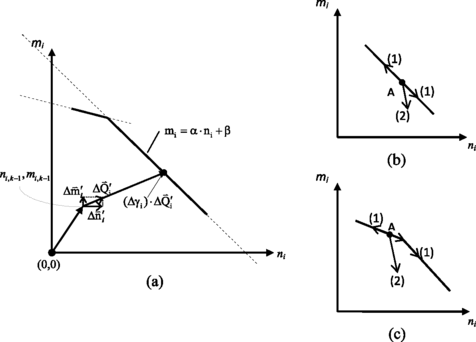

  

  (a) Search direction and plasticization from elastic state, (b) Further plasticization (1) or unloading (2)

• 5. Find the correct Δγ _k as the minimum Δγ _i,k among the non-active constraints that produces a new plastic hinge (Fig. 5(a)):

  $$ \Delta\gamma_{i,k} = \frac{(\alpha_{i} \cdot n_{i,k - 1} + \beta_{i}) - m_{i,k - 1}}{\Delta m'_{i} - \alpha_{i} \cdot \Delta n'_{i}} $$

  (16)

  where i=1,2,…N _c , with N _c being the total number of critical sections. The parameters (a _i ,β _i ) may be evaluated with the aid of (6) and turn out to be:

  $$\alpha_{i} = - \frac{s_{2}}{s_{1}} \cdot\frac{m_{*,i}}{n_{*,i}} \quad\text{and}\quad\beta_{i} = \frac{m_{*,i}}{s_{1}} $$

  A search is made for each critical section for all the possible intersections with the yield planes for all the four quadrants. The minimum positive among all numbers one may get using (16), is the sought Δγ _i,k .

• 6. Find the increments of the bending moments, axial forces and plastic displacements as:

  $$ \Delta\mathbf{m} = \Delta\gamma_{k} \cdot\Delta\mathbf{m}', \quad\Delta\mathbf{n} = \Delta\gamma_{k} \cdot\Delta\mathbf {n}',\quad \Delta\mathbf{q}^{pl} = \Delta\gamma_{k} \cdot\Delta\mathbf {q}^{\prime pl} $$

  (17)

• 7. The load factor, the various static and kinematic variables may be now updated:

  $$ \begin{aligned}[c] &\gamma_{k} = \gamma_{k - 1} + \Delta\gamma_{k} \\ &\left. \begin{array}{@{}l} \mathbf{m}_{k} = \mathbf{m}_{k - 1} + \Delta \mathbf{m} \\ \mathbf{n}_{k} = \mathbf{n}_{k - 1} + \Delta\mathbf{n} \end{array} \right\} \quad\mapsto\quad\mathbf{Q}_{k}\\ &\left. \begin{array}{@{}l} \boldsymbol{\theta} _{k}^{el} = \mathbf{F}_{m} \cdot\mathbf{m}_{k} \\ \boldsymbol{\delta} _{k}^{el} = \mathbf{F}_{n} \cdot\mathbf{n}_{k} \end{array} \right\}\quad \mapsto \quad\mathbf{q}_{k}^{el} = \bar{\mathbf{F}} \cdot\mathbf{Q}_{k}\\ & \mathbf{q}_{k}^{pl} = \mathbf{q}_{k - 1}^{pl} + \Delta\mathbf{q}^{pl} \\ &\mathbf{q}_{k} = \mathbf{q}_{k}^{el} + \mathbf{q}_{k}^{pl} \end{aligned} $$

  (18)

  The displacements at the points of the load application may be found from SKD:

  $$\mathbf{u}_{k} = \bar{\mathbf{B}}_{0}^{T} \cdot\mathbf{q}_{k} $$

• 8. Return to step 1 and repeat the process for k=k+1, until either

  • i. No solution of the QP may be found, meaning a collapse state has been reached and if it were for a limit analysis case γ _k is the limit load factor, or

  • ii. For a prescribed loading the process stops if (i) has not occurred and |γ _k−∥P _L ∥|≤ρ, meaning we have reached the end of the specific loading case.

If we have an already plasticized critical section, the algorithm automatically detects at the beginning of the incremental step whether we are going to move along the directions (1) (Fig. 5(b) or (c)), meaning we get further plasticization, or move along the directions (2), meaning we have plastic unloading. Moving along either the direction (1) or (2) depends on whether the corresponding Lagrange multiplier of the active constraint becomes positive or zero, respectively.

There is always going to be one active constraint for a particular critical section. Even in the case of Fig. 5(c) when further plasticization continues along a neighboring constraint the previously active one now becomes inactive. In the very unlikely case when the search direction meets the point of intersection of the two constraints, then two nonzero Lagrange multipliers Δλ _i will appear, rendering both the constraints active. Thus, because of (9), two plastic vectors will appear. Each of them is perpendicular to the corresponding plane. In this case the plastic deformation will be the composition of these two vectors.

A physical interpretation of the fictitious load factor that is used at the beginning of the incremental step is to find a feasible direction on which the prospective solution lies taking into account all the previous plasticization that have occurred before the current incremental step. The true length of the step is then found on the demand to capture the next plasticization. The procedure may be depicted for two steps on a force-displacement diagram of the Fig. 6.

Fig. 6

Search direction with fictitious (ρ), and true incremental load factors (Δγ)

5 Numerical Example

The numerical example has been chosen in order to demonstrate the efficiency of the approach. This example was found difficult to converge when using standard commercial packages that use the direct stiffness as the solution method [14, 15].

The structure is a three-storey one-bay frame shown in Fig. 7. The original frame has appeared with Imperial units [16] which herein have been converted to SI.

Fig. 7

Geometry of the analyzed frame

This frame was experimentally tested by Yarimci [17] and the results of the experiments have been taken from [16]. The members of the frame were assigned mechanical properties, which are shown in Table 1, so that they match the ones that were measured. A pure bending behavior was considered for the beams.

Table 1 Mechanical properties used for the analysis

The loading scenario is the following: First the vertical loads were applied up to their final values that may be seen in Fig. 7 and then the horizontal loads were proportionally increased from zero. These loads were applied up to a certain value, then unloading of the structure took place, following a reversed loading and then reloading up to zeros so that a full cycle of loading was completed.

Three different constitutive relations were considered: (a) a pure bending behavior (to all the members a big value for n _∗ was given as input), (b) a moment/axial interaction using the “M+N=1” criterion and (c) a moment/axial interaction using the AISC LRFD criterion [13].

For all the three different cases of constitutive modeling, the numerical application of loading, unloading and reloading tried to follow the experiment that was performed [16].

Results of the three analyses are shown in Fig. 8.

Fig. 8

Horizontal load in kN (vertical axis) vs. Roof Displacement in m (horizontal axis)

One may see that the pure bending behavior simulates better the loading part of the cycle. This supports the assumption that for low rise buildings moment/axial force interaction need not be considered. The residual bending moment diagram at the end of the load cycle may be seen in Fig. 9.

Fig. 9

Bending moment distribution at the end of the load cycle under pure bending

Although the conditions of the experiment are not known in great detail, it seems that, under the assumptions of an elastic-perfectly plastic material and first order theory, the analytical results underestimate, in terms of the load, the unloading part of the cycle.

On the other hand, when moment/axial force interaction under any of the two criteria is considered, the hysteresis loop shrinks. This supports the fact of the reduced ductility of a frame in the presence of axial forces.

In Figs. 10 & 11 one may see the residual bending moment and axial force distributions at the end of the loading cycle for the two criteria.

Fig. 10

Bending moment distributions at the end of the cycle under bending and axial force interactions

Fig. 11

Axial force distributions at the end of the cycle under bending and axial force interactions

5.1 Computational Considerations

The fictitious factor ρ is the basis of the presented method. In this way we may have the conversion of the PQP problem to a QP one. It is a pure number and in order to capture all the events, one has to use a small value. In all the examples that were tried, a value of 10⁻³ or 10⁻⁴ has proved to be sufficient.

6 Conclusions

The nonholonomic elastoplastic analysis is performed with the aid of the force method of analysis. The framework of the exposed method is mathematical programming with a strategy to convert the resulting program which is originally a parametric quadratic program to a pure quadratic program.

As demonstrated from the presented example and also from other examples that were tested [10] the method proves to be a very stable and robust numerical procedure.

It is also computationally efficient because the only matrix that needs to be formed and decomposed once and for all is the flexibility matrix. The quadratic program is solved only once at the beginning of each incremental step and the step length that determines the next plasticization is determined automatically without the need to perform unnecessary intermediate elastic steps that have fixed length as is the case in any computer program that has the direct stiffness method as the basis for its formulation. No elastic prediction-plastic correction and no reformulation or re-decomposition of any matrix, as it would be the case for the stiffness matrix in a direct stiffness method, is needed. This operation, which is well known to be quite time consuming, is also avoided in the case of plastic unstressing since this information is contained directly inside the solution of the quadratic program and no extra work needs to be done. Thus from comparisons that have been made with the orthodox time stepping direct stiffness methods it has proved to be much more reliable and efficient [10].

The method although is certainly a step-by-step procedure it may be classified as a direct method as it is formulated within mathematical programming. These methods are known to be better suited than the direct stiffness method based ones if one seeks for a limit state of a structure. It is hoped that such methods will also be used more and more in the future as they seem to be a better alternative, even for a historical deformation analysis of a structure.

References

Maier, G.: A quadratic programming approach for certain classes of non linear structural problems. Meccanica 3, 121–130 (1968)
Maier, G.: A matrix structural theory of piecewise linear elastoplasticity with interacting yield planes. Meccanica 5, 54–66 (1970)
De Donato, O., Maier, G.: Historical deformation analysis of elastoplastic structures as a parametric linear complementarity problem. Meccanica 11, 166–171 (1976)
Smith, D.L.: The Wolf-Markowitz algorithm for nonholonomic elastolpastic analysis. Eng. Struct. 1, 8–16 (1978)
Franchi, A., Cohn, M.Z.: Computer analysis of elastic-plastic structures. Comput. Methods Appl. Mech. Eng. 21, 271–294 (1980)
Kaneko, I.: Complete solutions for a class of elastic-plastic structures. Comput. Methods Appl. Mech. Eng. 21, 193–209 (1980)
Tangaramvong, S., Tin-Loi, F.: Limit analysis of strain softening steel frames under pure bending. J. Constr. Steel Res. 63, 1151–1159 (2007)
Tangaramvong, S., Tin-Loi, F.: A complementarity approach for elastoplastic analysis of strain softening frames under combined bending and axial force. Eng. Struct. 29, 742–753 (2007)
Tin-Loi, F., Wong, M.B.: Nonholonomic computer analysis of elastoplastic frames. Comput. Methods Appl. Mech. Eng. 72, 351–364 (1989)
Spiliopoulos, K.V., Patsios, T.N.: An efficient mathematical programming method for the elastoplastic analysis of frames. Eng. Struct. 32, 1199–1214 (2010)
Golfarb, D., Idnani, A.: A numerically stable dual method for solving strictly convex quadratic programs. Math. Program. 27, 1–33 (1983)
Spiliopoulos, K.V.: On the automation of the force method in the optimal plastic design of frames. Comput. Methods Appl. Mech. Eng. 141, 141–156 (1997)
American Institute of Steel Construction: Load and Resistance Factor Design Specification for Structural Steel Buildings, Chicago, 2nd edn. (1993)
SAP2000: ver. 14.1.0 User’s manual. CSI Inc. (2010)
ABAQUS: ver. 6.8-1 User’s manual. SIMULIA Inc. (2009)
Toma, S., Chen, W.-F., White, D.W.: A selection of calibration frames in North America for second-order inelastic analysis. Eng. Struct. 17, 104–112 (1995)
Yarimci, E.: Incremental inelastic analysis of framed structures and some experimental verifications. PhD dissertation, Department of Civil Engineering, Lehigh University, Bethlehem, PA (1966)
Author information
Authors and Affiliations
Corresponding author
Editor information
Editors and Affiliations
Rights and permissions
Copyright information
© 2013 Springer Science+Business Media Dordrecht
About this paper
Cite this paper
Spiliopoulos, K.V., Patsios, T.N. (2013). Numerical Analysis of Nonholonomic Elastoplastic Frames by Mathematical Programming. In: de Saxcé, G., Oueslati, A., Charkaluk, E., Tritsch, JB. (eds) Limit State of Materials and Structures. Springer, Dordrecht. https://doi.org/10.1007/978-94-007-5425-6_7
Download citation
DOI: https://doi.org/10.1007/978-94-007-5425-6_7
Publisher Name: Springer, Dordrecht
Print ISBN: 978-94-007-5424-9
Online ISBN: 978-94-007-5425-6
eBook Packages: EngineeringEngineering (R0)