Canonical Forms Applied to Structural Mechanics

Abstract

The main objective of this chapter is to illustrate different applications of the canonical forms in structural mechanics with particular emphasis on calculating the buckling load and eigenfrequencies of the symmetric structures.

These keywords were added by machine and not by the authors. This process is experimental and the keywords may be updated as the learning algorithm improves.

7.1 Introduction

The main objective of this chapter is to illustrate different applications of the canonical forms in structural mechanics with particular emphasis on calculating the buckling load and eigenfrequencies of the symmetric structures.

In the first part, the problem of finding eigenvalues and eigenvectors of symmetric mass–spring vibrating systems is transferred into calculating those of their modified subsystems. This decreases the size of the eigenvalue problems and correspondingly increases the accuracy of their solutions and reduces the computational time [1].

In the second part, a methodology is presented for efficient calculation of buckling loads for symmetric frame structures. This is achieved by decomposing a symmetric model into two submodels followed by their healing to obtain the factors of the model. The buckling load of the entire structure is then obtained by calculating the buckling loads of its factors [2].

In the third part, the graph models of planar frame structures with different symmetries are decomposed, and appropriate processes are designed for their healing in order to form the corresponding factors. The eigenvalues and eigenvectors of the entire structure are then obtained by evaluating those of its factors. The methods developed in this part simplify the calculation of the natural frequencies and natural modes of the planar frames with different types of symmetry [3].

In the fourth part, methods are presented for calculating the eigenfrequencies of structures. The first approach is graph theoretical and uses graph symmetry. The graph models are decomposed into submodels, and healing processes are employed such that the union of the eigenvalues of the healed submodels contains the eigenvalues of the entire model. The second method has an algebraic nature and uses special canonical forms [4].

In the fifth part, general forms are introduced for efficient eigensolution of special tri-diagonal and five-diagonal matrices. Applications of these forms are illustrated using problems from mechanics of structures [5].

In the sixth part, the decomposability conditions of matrices are studied. Matrices that can be written as the sum of three Kronecker products are studied; examples are included to show the efficiency of this decomposition approach [6].

In the seventh part, canonical forms are used to decompose the symmetric line elements (truss and beam elements) into sub-elements of less the number of degrees of freedom (DOFs). Then the matrices associated with each sub-element are formed, and finally the matrices associated with each subsystem are combined to form the matrices of the prime element [7].

In the final part, an efficient eigensolution is presented for calculating the buckling load and free vibration of rotationally cyclic structures [8]. This solution uses a canonical form linear algebra that often occurs in matrices associated with graph models. A substructuring method is proposed to avoid the generation of entire matrices. Utilising the aforementioned method, the geometric stiffness matrix is generated in an efficient time-saving manner. Then solution for the eigenproblem is presented for geometric nonlinearity via the canonical form based on block diagonalisation method.

7.2 Vibrating Cores for a Mass–Spring Vibrating System

Consider a symmetric system shown in Fig. 7.1a. This system is symmetric, and its properties can be studied using its substructures.

Fig. 7.1

A symmetric dynamic system and two subsystems with link spring

These properties consist of the mass ${{\mathrm{m}}_1}$ and the stiffness ${\mathrm{{k}}_1}$. The masses, stiffnesses and their connectivity are considered to be symmetric with respect to the axis shown in Fig. 7.1a.

This system can be considered as two identical subsystems connected to each other with a spring, knows as a link spring, as shown in Fig. 7.1b.

This system has two degrees of freedom v₁ and v₂. The natural frequencies and natural modes for the following eigenproblem

$$ \left\{ {[\mathbf{K}]-{\boldsymbol{\omega}^{{_2}}}[\mathbf{m}]} \right\}\{{\mathbf{\upphi}} \}=\{0\} $$

(7.1)

can be found as

$$ \left| {\ [\mathbf{K}]-{\omega^2}[\mathbf{m}]\ } \right|=0. $$

(7.2)

where [K] is the stiffness matrix and [m] is the mass matrix of the system. The eigenvalues and eigenvectors are denoted by ${\omega_\mathrm{{i}}}$ and ${\mathbf{\upphi}_\mathrm{{i}}}$, respectively.

Since [K] and [m] are both symmetric, therefore the matrix $\left[ {[\mathbf{K}]-{\omega^2}[\mathbf{m}]} \right]$ has Form II as the following:

$$ \left[ {\begin{array}{cccccc} {{\mathrm{{k}}_1}+{\mathrm{{k}}_2}-{\omega^2}{{\mathrm{m}}_1}} & {-{\mathrm{{k}}_2}} \\{-{\mathrm{{k}}_2}} & {{\mathrm{{k}}_1}+{\mathrm{{k}}_2}-{\omega^2}{{\mathrm{m}}_1}} \\\end{array}} \right]. $$

(7.3)

Using ${\omega^2}{{\mathrm{m}}_1}=\lambda$, one can write

$$ \left| {\left. {\begin{array}{cccccc} {({\mathrm{{k}}_1}+\mathrm{k}{}_2)-\lambda } & {-{\mathrm{{k}}_2}} \\{-{\mathrm{{k}}_2}} & {({\mathrm{{k}}_1}+{\mathrm{{k}}_2})-\lambda } \\\end{array}} \right|} \right.=0. $$

(7.4)

Since the stiffness matrix has Form II, thus one can find its eigenvalues by calculating those of its condensed submatrices

$$ \begin{array}{cccccc} \mathbf{C} =\left[ {{\mathrm{{k}}_1}+{\mathrm{{k}}_2}-{\mathrm{{k}}_2}} \right]=\left[ {{\mathrm{{k}}_1}} \right] \hfill \\\mathbf{D} =\;\left[ {{\mathrm{{k}}_1}+{\mathrm{{k}}_2}+{\mathrm{{k}}_2}} \right]=\left[ {{\mathrm{{k}}_1}+2{\mathrm{{k}}_2}} \right]. \hfill\end{array} $$

(7.5)

The matrices C and D partially contain the eigenvalues of S. Since these submatrices have a nature similar to that of the overall stiffness matrix, thus the condensed matrices C and D define the stiffness matrices of the subsystems as shown in Fig. 7.1.

The structure corresponding to the condensed submatrices are referred to as vibrating cores. These vibrating cores contain part of the properties of the vibrating system. Therefore, the eigenvalues and eigenvectors of the overall structure can be found using those of C and D subsystems, Fig. 7.2.

Fig. 7.2

Subsystems corresponding to condensed submatrices C and D

For the system S having N degrees of freedom, m and K are $\mathrm{N}\times \mathrm{N}$ matrices, and if the structure is symmetric, the corresponding submatrices will be $\frac{\mathrm{{N}}}{2}\times \frac{\mathrm{{N}}}{2}$.

For investigating the vibrating modes of S and vibrating cores, consider the following definitions:

Definition 1

Let matrix M be in Form II as follows:

$$ \mathbf{M}=\left[ {\begin{array}{cccccc} \mathbf{A} &{\vrule height 5pt depth 5pt} & \mathbf{B} \\\noalign{\hrule}\mathbf{B} &{\vrule height 10pt depth 5pt} & \mathbf{A} \\\end{array}} \right]. $$

(7.6)

Let the corresponding eigenvalues of M be ${\lambda_1},{\lambda_2},{\lambda_3},\ldots,{\lambda_\mathrm{{n}}}$ with eigenvectors being as ${\mathbf{\upphi}_1},{\mathbf{\upphi}_2},{\mathbf{\upphi}_3},\ldots,{\mathbf{\upphi}_\mathrm{{n}}}$. The eigenvectors can be classified into two groups:

• First group: those with eigenvectors having $\frac{\mathrm{{N}}}{2}$ repeated entries

• Second group: those with eigenvectors having $\frac{\mathrm{{N}}}{2}$ repeated entries with reverse signs

Definition 2

If matrix M has a symmetry in Form II, then the condensed matrices are

$$ \mathbf{C}=\mathbf{A}+\mathbf{B}\mathrm{and}\mathbf{D}=\mathbf{A}-\mathbf{B}. $$

(7.7)

The eigenvectors of C are of the first group type and those of D are of the second group type.

Therefore, if the eigenvectors for the eigenvalues of C (with $\frac{\mathrm{{N}}}{2}$ entries) are calculated, then those of M can easily be obtained by addition of $\frac{\mathrm{{N}}}{2}$ entries, and those of D with reversed signs should be added.

7.2.1 The Graph Model of a Mass–Spring System

The mathematical model of a dynamic system consists of masses and springs. These masses are connected by means of springs. As the mathematical model, a weighted graph is defined as follows:

• 1. The supports in the mathematical model are associated neutral nodes in the graph.

• 2. For each mass, a node of graph is associated, and its weight is taken as the magnitude of the mass.

• 3. An edge is considered for each spring, and its weight is taken as the stiffness of the spring.

As an example, the graph model G1 of a dynamic system shown in Fig. 7.3a is depicted in Fig. 7.3b.

Fig. 7.3

A dynamic system and its graph model. (a) A symmetric dynamic system. (b) Graph model G1 of the system

For a dynamic system, we have

$$ \mathbf{K}\mathbf{\upphi} ={{{\boldsymbol{\omega}}}^2}\mathbf{m}\mathbf{\upphi} \Rightarrow \left[ {\mathbf{K}-{{{\boldsymbol{\omega}}}^2}\mathbf{m}} \right]\mathbf{\upphi} =\mathbf{0}. $$

(7.8)

This is an eigenvalue problem for which ω is the eigenvalue and $\mathbf{\upphi}$ is its eigenvector.

If we assume m as a diagonal matrix, then its inverse can easily be found, and we will have

$$\bf{m}^-{^1}{\bf{K\bf{\phi}}}=\bf{m}^-{^1}{{\bf{\omega}^2\bf m\bf{\phi}\Rightarrow}}\bf{m}^-{^1}{\bf{K\bf{\phi}}}={{\bf{\omega}^2\bf{\phi}\Rightarrow}}[\bf{m}^-{{^1\bf K}}-{{\bf{\omega}^2\bf I}}]{\bf{\phi}}={\bf {0}}. $$

(7.9)

If $[\mathbf{m}^-{^1}\mathbf{K}]=[{{\mathbf{L}}_\mathrm{{T}}}]$ and ${{{\lambda}}={{\omega^2}}}$, then we have

$$ \left[ {{{\mathbf{L}}_\mathrm{{T}}}-\lambda \mathbf{I}} \right]{\mathbf{\upphi} =\bf0}. $$

(7.10)

This is an eigenvalue problem corresponding to eigenvalues and eigenvectors of L _T. This relationship can be associated with the corresponding graph. If L _T is the generalised Laplacian of the graph, then the above problem becomes an eigenproblem of a graph.

7.2.2 Vibrating Systems with Form II Symmetry

As an example, the generalised Laplacian matrix for the graph G1 in Fig. 7.3 has the following form:

$$ {{\mathbf{L}}_\mathrm{{T}}}=\left[ {\begin{array}{cccccc} {{\mathrm{{k}}_1}+{\mathrm{{k}}_2}-{{\mathrm{m}}_1}} &{\vrule height 8pt depth 6pt} & {-{\mathrm{{k}}_2}} \\\noalign{\hrule} {-{\mathrm{{k}}_2}} &{\vrule height 8pt depth 6pt} & {{\mathrm{{k}}_1}+{\mathrm{{k}}_2}-{{\mathrm{m}}_1}} \\\end{array}} \right] $$

(7.11)

For a symmetric graph, an appropriate numbering of the nodes results in a generalised Laplacian matrix with Form II.

Example 7.1

Consider a dynamic system as shown in Fig. 7.4 with graph model being G2.

Fig. 7.4

A dynamic system and its graph model

This graph is symmetric and its Laplacian and generalised matrices are as follows:

$$ \mathbf{L}=\left[ {\begin{array}{cccccc} {{\mathrm{{k}}_1}+{\mathrm{{k}}_2}+{\mathrm{{k}}_3}} & {-{\mathrm{{k}}_2}} &{\vrule height 8pt depth 4pt} & {-{\mathrm{{k}}_3}} & 0 \cr\noalign{} {-{\mathrm{{k}}_2}} & {{\mathrm{{k}}_2}+{\mathrm{{k}}_3}} &{\vrule height 8pt depth 4pt} & 0 & {-{\mathrm{{k}}_3}} \cr\noalign{} \noalign{\hrule} {-{\mathrm{{k}}_3}} & 0 &{\vrule height 8pt depth 4pt} & {{\mathrm{{k}}_1}+{\mathrm{{k}}_2}+{\mathrm{{k}}_3}} & {-{\mathrm{{k}}_2}} \cr\noalign{} 0 & {-{\mathrm{{k}}_3}} &{\vrule height 8pt depth 4pt} & {-{\mathrm{{k}}_2}} & {{\mathrm{{k}}_2}+{\mathrm{{k}}_3}} \\\end{array}} \right] $$

(7.12)

$$ {{\mathbf{L}}_\mathrm{{T}}}=\left[ {\begin{array}{cccccc} {{\mathrm{{k}}_1}+{\mathrm{{k}}_2}+{\mathrm{{k}}_3}-{{\mathrm{m}}_1}} & {-{\mathrm{{k}}_2}} &{\vrule height 8pt depth 4pt} & {-{\mathrm{{k}}_3}} & 0 \cr\noalign{} {-{\mathrm{{k}}_2}} & {{\mathrm{{k}}_2}+{\mathrm{{k}}_3}-{{\mathrm{m}}_2}} &{\vrule height 8pt depth 4pt} & 0 & {-{\mathrm{{k}}_3}} \cr\noalign{} \noalign{\hrule} {-{\mathrm{{k}}_3}} & 0 &{\vrule height 8pt depth 4pt} & {{\mathrm{{k}}_1}+{\mathrm{{k}}_2}+{\mathrm{{k}}_3}-{{\mathrm{m}}_1}} & {-{\mathrm{{k}}_2}} \cr\noalign{} 0 & {-{\mathrm{{k}}_3}} &{\vrule height 8pt depth 4pt} & {-{\mathrm{{k}}_2}} & {{\mathrm{{k}}_2}+{\mathrm{{k}}_3}-{{\mathrm{m}}_2}} \\\end{array}} \right]. $$

(7.13)

For the symmetry in Form II, the generalised Laplacian matrix can be written as

$$ {{\mathbf{L}}_\mathrm{{T}}}=\left[ {\begin{array}{cccccc} \mathbf{S} &{\vrule height 8pt depth 4pt} & {\mathbf{L}\mathbf{I}} \cr\noalign{} \noalign{\hrule} {\mathbf{L}\mathbf{I}} &{\vrule height 8pt depth 4pt} & \mathbf{S} \\\end{array}} \right]. $$

(7.14)

The submatrix S is called the shape matrix and represents the properties of both subgraphs, which are identical, and LI is called the link matrix and shows the way two subgraphs are connected to each other. The submatrix LI represents the effect of the springs between two subgraphs in the stiffness matrix.

As mentioned before, we have an eigenproblem for the matrix L _T. According to the properties of Form II, if $[\mathbf{S}+\mathbf{LI}] = \mathbf{C}$ and $[\mathbf{S}-\mathbf{LI}] = \mathbf{D}$, then ${{{\mathbf{L}}^{\prime}}_\mathrm{{T}}}$ can be expressed as

$$ {{{\mathbf{L}}^{^\prime}}_\mathrm{{T}}}=\left[ {\begin{array}{cccccc} \mathbf{C} & \mathbf{0} \\\mathbf{0} & \mathbf{D} \\\end{array}} \right]. $$

(7.15)

If ${{{\mathbf{L}}^{\prime}}_\mathrm{{T}}}$ is the generalised Laplacian matrix of a graph, then this graph will consist of two subgraphs with N/2 nodes for each subgraph which are not connected to each other, and L _T has eigenvalues as

$$ \mathrm{EIG}({{\mathbf{L}}_\mathrm{{T}}})=\mathrm{EIG}(\mathbf{C})\cup \mathrm{EIG}(\mathbf{D}). $$

(7.16)

Thus, the subgraphs C and D are the dynamic cores of the model. Each core defines part of the natural frequencies ${\boldsymbol{{\omega}}_\mathrm{{i}}}$ of the entire system.

$$ \left\{ {{\boldsymbol{\omega}_{{{{\mathbf{L}}_\mathrm{{T}}}}}}} \right\}=\left\{ {{\boldsymbol{\omega}_\mathrm{{D}}}} \right\}\cup \left\{ {{\boldsymbol{\omega}_\mathrm{{E}}}} \right\}. $$

(7.17)

As an example, for graph G2, the cores C and D are shown in Fig. 7.5.

Fig. 7.5

The dynamic cores C and D of G2

Laplacian matrices of C and D are as follows:

$$ {{\mathbf{L}}_C}=\left[ {\begin{array}{cccccc} {{\mathrm{{k}}_1}+{\mathrm{{k}}_2}} & {-{\mathrm{{k}}_2}} \\{-{\mathrm{{k}}_2}} & {{\mathrm{{k}}_2}} \\\end{array}} \right] $$

(7.18)

and

$$ {{\mathbf{L}}_{\rm D}}=\left[ {\begin{array}{cccccc} {{\mathrm{{k}}_1}+{\mathrm{{k}}_2}+2{\mathrm{{k}}_3}} & {-{\mathrm{{k}}_2}} \\{-{\mathrm{{k}}_2}} & {{\mathrm{{k}}_2}+2{\mathrm{{k}}_3}} \\\end{array}} \right] $$

(7.19)

As mentioned previously, the Laplacian matrix of the corresponding graphs is the same as the stiffness matrices of the mathematical model for each subgraph C and D as shown in Fig. 7.6.

Fig. 7.6

The mathematical models for C and D

7.2.3 Vibrating Systems with Form III Symmetry

For a symmetric system with odd number of masses, the corresponding graph will have Form III symmetry. For such a system, the vibrating cores can be identified using symmetry.

As the third example, consider the model shown in Fig. 7.7a.

Fig. 7.7

A dynamic system and its graph model

The corresponding graph is shown in Fig. 7.7b.

The Laplacian and generalised Laplacian matrices are as follows:

$$ \mathbf{L}=\left[ {\begin{array}{cccccc} {{\mathrm{{k}}_1}+{\mathrm{{k}}_2}} & 0 & {-{\mathrm{{k}}_2}} \\0 & {{\mathrm{{k}}_1}+{\mathrm{{k}}_2}} & {-{\mathrm{{k}}_2}} \\{-{\mathrm{{k}}_2}} & {-{\mathrm{{k}}_2}} & {2{\mathrm{{k}}_2}} \\\end{array}} \right], $$

(7.20)

$$ {{\mathbf{L}}_{\mathrm{T}}}=\left[ \begin{gathered} \left. {\underline{\, {\begin{array}{*{20}{c}} {{{\mathrm{k}}_1} + {{\mathrm{k}}_2}-{{\mathrm{m}}_1}} & 0 \\ 0 & {{{\mathrm{k}}_1}+{{\mathrm{k}}_2}-{{\mathrm{m}}_1}} \\ \end{array}}\,}} \! \right|\begin{array}{*{20}{c}} {-{{\mathrm{k}}_2}} \\ {-{{\mathrm{k}}_2}} \\ \end{array} \hfill \\ \begin{array}{*{20}{c}} \qquad{-{{\mathrm{k}}_2}} & \qquad\qquad{-{{\mathrm{k}}_2}} &\quad {2{{\mathrm{k}}_2}-{{\mathrm{m}}_2}} \\ \end{array} \hfill \\ \end{gathered} \right].$$

(7.21)

As it can be seen, both L and L _T have Form III.

The Laplacian matrices corresponding to the vibrating cores are given below:

$$ {{\mathbf{L}}_D}=[{\mathrm{{k}}_1}+{\mathrm{{k}}_2}-0]=[{\mathrm{{k}}_1}+{\mathrm{{k}}_2}], $$

(7.22)

and

$$ {{\mathbf{L}}_\mathrm{{E}}}=\left[ {\begin{array}{cccccc} {{\mathrm{{k}}_1}+{\mathrm{{k}}_2}} & {-{\mathrm{{k}}_2}} \\{-2{\mathrm{{k}}_2}} & {2{\mathrm{{k}}_3}} \\\end{array}} \right]. $$

(7.23)

The graphs of these matrices are shown in Fig. 7.8.

Fig. 7.8

The subgraphs for D and E

If there is a directed edge between two nodes i and j directed from i to j, it represents a directed spring in the dynamic system, Fig. 7.9. The main characteristic of such a spring is that the connection of this spring to masses is such that it does not take part in the stiffness of k_j,i, but it effects the k_i,j, that is,

Fig. 7.9

A directed spring

The mathematical models corresponding to the cores D and E are shown in Fig. 7.10.

Fig. 7.10

Models corresponding to D and E

According to the properties of the cores,

$$ \left\{ {\lambda {{\mathbf{L}}_\mathrm{{T}}}} \right\}=\left\{ {{\lambda_{{D}}}} \right\}\cup \left\{ {{\lambda_{{E}}}} \right\}, $$

(7.24)

and

$$ \left\{ {\omega {{\mathbf{L}}_\mathrm{{T}}}} \right\}=\left\{ {{\omega_{{D}}}} \right\}\cup \left\{ {{\omega_{{E}}}} \right\}. $$

(7.25)

and from the vibrating cores E and D, the natural modes of the entire system can be found.

If each a vibrating system contains symmetry, then the cores can be decomposed accordingly. Further decomposition of the refined cores for symmetry is also possible.

7.2.4 Generalized Form III and Vibrating System

As described in Chap. 4, for a graph with symmetric core having Form III, if the complement of the core is connected by the nodes of degree 1, then the nodes can be ordered to produce a Laplacian matrix of Form III. This property can also be used for graphs corresponding to the vibrating systems.

Consider the system in Fig. 7.11a together with its graph being illustrated in Fig. 7.11b.

Fig. 7.11

A dynamic system and its graph model

The subgraph containing the nodes A, B and C has a symmetric core of Form III. The nodes E and D are connected to this core through C. Therefore, the Laplacian matrix of this graph will be in the generalised Form III. L and L _T are formed as follows:

$$ \mathbf{L}=\left[ {\begin{array}{cccccc} {{\mathrm{{k}}_1}+{\mathrm{{k}}_2}} & {-{\mathrm{{k}}_1}} & {-{\mathrm{{k}}_2}} & 0 & 0 \\{-{\mathrm{{k}}_1}} & {{\mathrm{{k}}_1}+{\mathrm{{k}}_2}} & {-{\mathrm{{k}}_2}} & 0 & 0 \\{-{\mathrm{{k}}_2}} & {-{\mathrm{{k}}_2}} & {2{\mathrm{{k}}_2}+{\mathrm{{k}}_3}} & {-{\mathrm{{k}}_3}} & 0 \\0 & 0 & {-{\mathrm{{k}}_3}} & {{\mathrm{{k}}_3}+{\mathrm{{k}}_4}} & {-{\mathrm{{k}}_4}} \\0 & 0 & 0 & {-{\mathrm{{k}}_4}} & {{\mathrm{{k}}_4}+{\mathrm{{k}}_5}} \\\end{array}} \right], $$

(7.26)

$$ {{\mathbf{L}}_\mathrm{{T}}}=\left[ {\begin{array}{cccccc} {{\mathrm{{k}}_1}+{\mathrm{{k}}_2}-{{\mathrm{m}}_1}} & {-{\mathrm{{k}}_1}} & {-{\mathrm{{k}}_2}} & 0 & 0 \\{-{\mathrm{{k}}_1}} & {{\mathrm{{k}}_1}+{\mathrm{{k}}_2}-{{\mathrm{m}}_1}} & {-{\mathrm{{k}}_2}} & 0 & 0 \\{-{\mathrm{{k}}_2}} & {-{\mathrm{{k}}_2}} & {2{\mathrm{{k}}_2}+{\mathrm{{k}}_3}-{{\mathrm{m}}_2}} & {-{\mathrm{{k}}_3}} & 0 \\0 & 0 & {-{\mathrm{{k}}_3}} & {{\mathrm{{k}}_3}+{\mathrm{{k}}_4}-{{\mathrm{m}}_3}} & {-{\mathrm{{k}}_4}} \\0 & 0 & 0 & {-{\mathrm{{k}}_4}} & {{\mathrm{{k}}_4}+{\mathrm{{k}}_5}-{{\mathrm{m}}_4}} \\\end{array}} \right]. $$

(7.27)

The connected submatrices D and E are formed for L _T as

$$ \mathbf{D}=\left[ {{\mathrm{{k}}_1}+{\mathrm{{k}}_2}-{{\mathrm{m}}_1}-\left( {-{\mathrm{{k}}_1}} \right)} \right]=\left[ {2{\mathrm{{k}}_1}+{\mathrm{{k}}_2}-{{\mathrm{m}}_1}} \right], $$

(7.28)

$$ \mathbf{E}=\left[ {\begin{array}{cccccc} {{\mathrm{{k}}_1}+{\mathrm{{k}}_2}-{{\mathrm{m}}_1}-{\mathrm{{k}}_1}} & {-{\mathrm{{k}}_2}-{\mathrm{{k}}_2}} & 0 & 0 \\{-{\mathrm{{k}}_2}-{\mathrm{{k}}_2}} & {2{\mathrm{{k}}_2}+{\mathrm{{k}}_3}-{{\mathrm{m}}_2}} & {-{\mathrm{{k}}_3}} & 0 \\0 & {-{\mathrm{{k}}_3}} & {{\mathrm{{k}}_3}+{\mathrm{{k}}_4}-{{\mathrm{m}}_3}} & {-{\mathrm{{k}}_4}} \\0 & 0 & {-{\mathrm{{k}}_4}} & {{\mathrm{{k}}_4}+{\mathrm{{k}}_5}-{{\mathrm{m}}_4}} \\\end{array}} \right], $$

(7.29)

or

$$ \mathbf{E}=\left[ {\begin{array}{cccccc} {{\mathrm{{k}}_2}-{{\mathrm{m}}_1}} & {-{\mathrm{{k}}_2}} & 0 & 0 \\{-2{\mathrm{{k}}_2}} & {2{\mathrm{{k}}_2}+{\mathrm{{k}}_3}-{{\mathrm{m}}_2}} & {-{\mathrm{{k}}_3}} & 0 \\0 & {-{\mathrm{{k}}_3}} & {{\mathrm{{k}}_3}+{\mathrm{{k}}_4}-{{\mathrm{m}}_3}} & {-{\mathrm{{k}}_4}} \\0 & 0 & {-{\mathrm{{k}}_4}} & {{\mathrm{{k}}_4}+{\mathrm{{k}}_5}-{{\mathrm{m}}_4}} \\\end{array}} \right]. $$

(7.30)

The subgraphs associated with the cores D and E are shown in Fig. 7.12.

Fig. 7.12

Subgraphs D and E

The form of the vibrating cores corresponding to D and E is shown in Fig. 7.13.

Fig. 7.13

Submodels D and E

It can be observed that due to the symmetry, the generalised Laplacian is decomposed into two submatrices of 1 × 1 and 4 × 4, and the cores are formed.

If N other nodes are connected to C in a similar manner, again the graph can be decomposed into two cores D and E, as shown in Fig. 7.14. It should be noted that the core D does not change.

Fig. 7.14

A graph decomposable into D and E

Thus, the natural frequency of the core D and the corresponding mode of the system will be unaltered. Therefore, one can conclude that part of the natural frequency of the symmetric system with Form III will exactly be reflected in the whole system.

Consider the system shown in Fig. 7.15.

Fig. 7.15

A dynamic system and its graph model

The L _T, L _D and L _E matrices are as follows:

$$ \begin{array}{cccccc} \begin{array}{cccccc} {\kern3.75em \mathrm{A}} & {\kern4.25em \mathrm{B}} & {\kern3.75em \mathrm{C}} & {\kern3.5em \mathrm{D}} & {\kern3.75em \mathrm{E}} & {\kern3.25em \mathrm{F} } \cr\end{array} \hfill \\{{\mathbf{L}}_\mathrm{{T}}}=\left[ {\begin{array}{cccccc} {{\mathrm{{k}}_1}+{\mathrm{{k}}_3}-{{\mathrm{m}}_1}} & {-{\mathrm{{k}}_1}} & 0 & 0 & {-{\mathrm{{k}}_3}} & 0 \\{-{\mathrm{{k}}_1}} & {{\mathrm{{k}}_1}+{\mathrm{{k}}_2}-{{\mathrm{m}}_1}} & 0 & {-{\mathrm{{k}}_2}} & 0 & 0 \\0 & 0 & {{\mathrm{{k}}_1}+{\mathrm{{k}}_3}-{{\mathrm{m}}_1}} & {-{\mathrm{{k}}_1}} & {-{\mathrm{{k}}_3}} & 0 \\0 & {-{\mathrm{{k}}_2}} & {-{\mathrm{{k}}_1}} & {{\mathrm{{k}}_1}+{\mathrm{{k}}_2}-{{\mathrm{m}}_1}} & 0 & 0 \\{-{\mathrm{{k}}_3}} & 0 & {-{\mathrm{{k}}_3}} & 0 & {2{\mathrm{{k}}_3}+{\mathrm{{k}}_4}-{{\mathrm{m}}_2}} & {-{\mathrm{{k}}_4}} \\0 & 0 & 0 & 0 & {-{\mathrm{{k}}_4}} & {{\mathrm{{k}}_4}+{\mathrm{{k}}_5}-{{\mathrm{m}}_3}} \\\end{array}} \right] \hfill\end{array} $$

(7.31)

$$ {{\mathbf{L}}_\mathrm{{D}}}=\left[ {\begin{array}{cccccc} {{\mathrm{{k}}_1}+{\mathrm{{k}}_3}-{{\mathrm{m}}_1}} & {-{\mathrm{{k}}_1}} \\{-{\mathrm{{k}}_1}} & {{\mathrm{{k}}_1}+2{\mathrm{{k}}_2}-{{\mathrm{m}}_1}} \\\end{array}} \right]. $$

(7.32)

And the corresponding graph and model are illustrated in Fig. 7.16.

Fig. 7.16

The submodel D and the corresponding subgraph

Also we have

$$ {{\mathbf{L}}_\mathrm{{E}}}=\left[ {\begin{array}{cccccc} {{\mathrm{{k}}_1}+{\mathrm{{k}}_3}-{{\mathrm{m}}_1}} & {-{\mathrm{{k}}_1}} & {-{\mathrm{{k}}_3}} & 0 \\{-{\mathrm{{k}}_1}} & {{\mathrm{{k}}_1}-{{\mathrm{m}}_1}} & 0 & 0 \\{-2{\mathrm{{k}}_3}} & 0 & {2{\mathrm{{k}}_3}+{\mathrm{{k}}_4}-{{\mathrm{m}}_2}} & {-{\mathrm{{k}}_4}} \\0 & 0 & {-{\mathrm{{k}}_4}} & {{\mathrm{{k}}_4}+{\mathrm{{k}}_5}-{{\mathrm{m}}_3}} \\\end{array}} \right]. $$

(7.33)

And the corresponding model and graph are shown in Fig. 7.17.

Fig. 7.17

The submodel E and the corresponding subgraph

7.2.5 Discussion

Symmetry of a mathematical model corresponds to the symmetric distribution of the physical properties comprising of masses and stiffnesses of the springs and the connectivity of the masses by means of springs.

For the graph model of a dynamic system, symmetry of Form II results in two vibrating cores C and D. These cores are physically identified with the difference of C being more flexible than D, and the main frequency and the corresponding mode are contained in this part of the model.

For the graph model of a vibrating system having Form III symmetry, the two vibrating cores D and E are produced. The number of masses and springs in D is less than E, and directed springs are included in the core E.

Although the systems studied in here are mass–spring systems, however, the application of the present method can be extended to other structural systems. The application can also be extended to stability analysis of frame structures.

7.3 Buckling Load of Symmetric Frames

In this part a method is presented for efficient calculation of buckling loads for symmetric frame structures. This is achieved by decomposing a symmetric model into two submodels followed by their healing to obtain the factors of the model. The buckling load of the entire structure is then obtained by calculating the buckling loads of its factors.

7.3.1 Buckling Load for Symmetric Frames with Odd Number of Spans per Storey

In this section, symmetric frames with an odd number of spans per storey are studied. The axis of symmetry for these structures passes through the central beams. For these frames, the matrices have canonical Form II patterns.

Non-sway Frames: Frames with no sway have no lateral displacement, and only rotational DOF specifies the deformation of the structure. In this study, for rigid-jointed frames in each joint, one rotational degree of freedom is considered.

For non-sway frames with odd number of spans per storey, if the loading is also symmetric, then the stiffness matrix with an appropriate numbering of the DOF will have canonical Form II pattern. In this case, the structure has two factors, one of which is stiffer than the other. Naturally the weaker factor will have smaller buckling load. Therefore, in order to find the buckling load for such a frame, with N DOF, it is sufficient to calculate the buckling load of a weaker factor with N/2 DOF. This process reduces the computational time and the necessary storage.

Decomposition and Healing Process: The operations performed after decomposition is called the healing of substructures. The submodels obtained after the decomposition and healing are known as the factors of the structural model.

Healing for different types of symmetry requires different operations. These operations are designed such that the resulting factors correspond to the aforementioned condensed submatrices of the canonical forms.

For the non-sway frame with odd number of spans per storey, healing consists of the following steps:

• Step 1. Delete the beams which are crossed by the axis of symmetry. These are link beams and are identified by Lb. Now the structure is decomposed into two substructures S₁ and S₂ in the left- and right-hand sides, respectively.

• Step 2. For S₁, add one rotational spring, with a stiffness equal to $\frac{{6\mathrm{E}{\mathrm{{I}}_\mathrm{{lb}}}}}{\mathrm{{L}_\mathrm{{L}\mathrm{b}}^3}}={\mathrm{{k}}_\mathrm{{Ci}}}$, to the joint at the ith storey. This provides the necessary stiffness requirement for obtaining the factor C.

• Step 3. Add a rotational spring to S₂, with a stiffness of magnitude $\frac{{2\mathrm{E}{\mathrm{{I}}_\mathrm{{lb}}}}}{\mathrm{{L}_\mathrm{{L}\mathrm{b}}^3}}={\mathrm{{k}}_\mathrm{{Di}}}$, at the joint of the ith storey. This provides the necessary stiffness requirement for obtaining the factor D.

S₁ and S₂ are now healed and the factors C and D are obtained.

The reason for selecting such stiffnesses for the springs is discussed by the following simple example.

Example 7.2

Consider a simple symmetric portal frame with symmetric buckling mode as shown in Fig. 7.18.

Fig. 7.18

A simple symmetric bending frame

The stiffness matrix of the element with the numbering of the DOF as illustrated in Fig. 7.19 is formed using the standard stiffness method.

Fig. 7.19

Numbering of the DOF for a beam column

$$ \mathbf{k}=\frac{\mathrm{{EI}}}{{{\mathrm{{L}}^3}}}\left[ {\begin{array}{cccccc} {12} & {-6} &{\vrule height 8pt depth 4pt} & {-12} & 6 \cr\noalign{} {-6} & 4 &{\vrule height 8pt depth 4pt} & 6 & {-2} \cr\noalign{} \noalign{\hrule} {-12} & 6 &{\vrule height 8pt depth 4pt} & {12} & {-6} \cr\noalign{} 6 & {-2} &{\vrule height 8pt depth 4pt} & {-6} & 4 \\\end{array}} \right]-\frac{\mathrm{{P}}}{\mathrm{{L}}}\left[ {\begin{array}{cccccc} {\frac{6}{5}} & {\frac{-1 }{10 }} &{\vrule height 9pt depth 6pt} & {\frac{-6 }{5}} & {\frac{1}{10 }} \cr\noalign{} {\frac{-1 }{10 }} & {\frac{2}{15 }} &{\vrule height 9pt depth 6pt} & {\frac{1}{10 }} & {\frac{1}{30 }} \cr\noalign{} \noalign{\hrule} {\frac{-6 }{5}} & {\frac{-1 }{10 }} &{\vrule height 9pt depth 6pt} & {\frac{6}{5}} & {\frac{-1 }{10 }} \cr\noalign{} {\frac{-1 }{10 }} & {\frac{1}{30 }} &{\vrule height 9pt depth 6pt} & {\frac{-1 }{10 }} & {\frac{2}{15 }} \\\end{array}} \right]. $$

(7.34)

For the entire structure, the stiffness matrix is constructed as

$$ \mathbf{K}=\frac{\mathrm{{EI}}}{{{\mathrm{{L}}^3}}}\left[ {\begin{array}{cccccc} {8-4\lambda } &{\vrule height 8pt depth 4pt} & 2 \cr\noalign{} \noalign{\hrule} 2 &{\vrule height 8pt depth 4pt} & {8-4\lambda } \\\end{array}} \right],\mathrm{where}\ \ \lambda =\frac{\mathrm{{P}{\mathrm{{L}}^2}}}{{30\mathrm{EI}}}. $$

(7.35)

The numbering of the DOF should be such that the difference between symmetric DOF becomes N/2.

The condensed submatrices of K are

$$ \begin{array}{cccccc} \mathbf{A}-\mathbf{B}=\left[ {\frac{{6\mathrm{EI}}}{{{\mathrm{{L}}^3}}}-\frac{{4\mathrm{EI}}}{{{\mathrm{{L}}^3}}}\times \frac{\mathrm{{P}{\mathrm{{L}}^2}}}{{30\mathrm{EI}}}} \right]=\frac{\mathrm{{EI}}}{{{\mathrm{{L}}^3}}}[6-4\lambda ]\ \mathrm{and} \hfill \\\mathbf{A}+\mathbf{B}=\left[ {\frac{{10\mathrm{EI}}}{{{\mathrm{{L}}^3}}}-\frac{{4\mathrm{EI}}}{{{\mathrm{{L}}^3}}}\times \frac{\mathrm{{P}{\mathrm{{L}}^2}}}{{30\mathrm{EI}}}} \right]=\frac{\mathrm{{EI}}}{{{\mathrm{{L}}^3}}}[10-4\lambda ], \hfill\end{array} $$

(7.36)

corresponding to the factors D and C, respectively.

Design of the Factor D: A factor for which the stiffness matrix is $\left[ {\frac{{6\mathrm{EI}}}{{{\mathrm{{L}}^3}}}-\frac{{4\mathrm{EI}}}{{{\mathrm{{L}}^3}}}\times \frac{\mathrm{{P}{\mathrm{{L}}^2}}}{{30\mathrm{EI}}}} \right]$ may be considered as a column under axial load P, with a spring of stiffness ${\mathrm{{k}}_\mathrm{{C}}}=\frac{{6\mathrm{EI}}}{{{\mathrm{{L}}^3}}}$.

Design of the Factor C: Similarly, a factor for which the stiffness matrix is $\left[ {\frac{{10\mathrm{EI}}}{{{\mathrm{{L}}^3}}}-\frac{{4\mathrm{EI}}}{{{\mathrm{{L}}^3}}}\times \frac{\mathrm{{P}{\mathrm{{L}}^2}}}{{30\mathrm{EI}}}} \right]$ can be taken as a column under axial load P with a spring of stiffness ${\mathrm{{k}}_\mathrm{{D}}}=\frac{{10\mathrm{EI}}}{{{\mathrm{{L}}^3}}}$.

In order to determine the buckling load of the frame, the determinant of the stiffness matrix is equated to zero:

$$ \begin{array}{cccccc} \det \mathbf{K}= \det[\mathbf{A}-\mathbf{B}]\times \det[\mathbf{A}+\mathbf{B}]=0 \hfill \\\ \left| {6-4\lambda } \right|=0\ \mathrm{and}\;\left| {10-4\lambda } \right|=0 \hfill\end{array} $$

(7.37)

leading to

$$ {\lambda_1}=1.5\kern0.5em \mathrm{and}\ {\lambda_2}=2.5. $$

Therefore,

$$ {\lambda_{\min }}=1.5=\frac{{{\mathrm{{P}}_\mathrm{{cr}}}{\mathrm{{L}}^2}}}{{30\mathrm{EI}}}\ \mathrm{leading}\ \mathrm{to}{\mathrm{{P}}_\mathrm{{cr}}}=\frac{{45\mathrm{EI}}}{{{\mathrm{{L}}^2}}}. $$

Alternative Solution: First the factors are formed as shown in Fig. 7.20. The buckling load of the structure is obtained by finding the buckling load of the factor D.

Fig. 7.20

Factors of the structure S. (a) Factor C (b) Factor D

$$ \begin{array}{cccccc} {{\mathbf{K}}_\mathrm{{C}}}=\left[ {\frac{{2\mathrm{EI}}}{{{\mathrm{{L}}^3}}}(2)+\frac{{6\mathrm{EI}}}{{{\mathrm{{L}}^3}}}-\frac{{2\mathrm{P}}}{{15\mathrm{L}}}} \right]=\left[ {\frac{{10\mathrm{EI}}}{{{\mathrm{{L}}^3}}}-\frac{{2\mathrm{P}}}{{15\mathrm{L}}}} \right] \hfill \\ {{\mathbf{K}}_\mathrm{{D}}}=\left[ {\frac{{2\mathrm{EI}}}{{{\mathrm{{L}}^3}}}(2)+\frac{{2\mathrm{EI}}}{{{\mathrm{{L}}^3}}}-\frac{{2\mathrm{P}}}{{15\mathrm{L}}}} \right]=\left[ {\frac{{6\mathrm{EI}}}{{{\mathrm{{L}}^3}}}-\frac{{2\mathrm{P}}}{{15\mathrm{L}}}} \right] \hfill\end{array} $$

(7.38)

Equating the determinant of K _D to zero, the same buckling load is obtained. This approximation is very crude and can be improved by considering each column as two or more elements. As an example, the columns with two elements are considered as shown in Fig. 7.21.

Fig. 7.21

A portal frame with six DOFs

Now the structure consists of four rotational degrees of freedom and two translation degrees of freedom. The corresponding stiffness matrix is obtained as

$$ \mathbf{K}=\frac{{8\mathrm{EI}}}{{{{\mathrm{L}}^3}}}\left[ {\begin{array}{*{20}{c}} {24-72\lambda } & 0 & {-6+3\lambda } & \vline & 0 & 0 & 0 \\ 0 & {8-8\lambda } & {2+\lambda } &\vline & 0 & 0 & 0 \\ {-6+3\lambda } & {2+\lambda } & {\tfrac{1}{2}+4-4\lambda } &\vline & 0 & 0 & {\tfrac{1}{4}} \\ \hline 0 & 0 & 0 &\vline & {24-72\lambda } & 0 & {-6+3\lambda } \\ 0 & 0 & 0 &\vline & 0 & {8-8\lambda } & {2+\lambda } \\ 0 & 0 & {\tfrac{1}{4}} &\vline & {-6+3\lambda } & {2+\lambda } & {\tfrac{1}{2}+4-4\lambda } \\ \end{array}} \right] $$

(7.39)

where $\lambda =\displaystyle\frac{\mathrm{{P}{\mathrm{{L}}^2}}}{{120\mathrm{EI}}}$.

Forming the determinants of A + B and A − B and equating to zero results in ${\lambda_{\min }}=0.185$ corresponding to ${\mathrm{{P}}_\mathrm{{cr}}}=\displaystyle\frac{{22.21\mathrm{EI}}}{{{\mathrm{{L}}^2}}}$ which is quite close to the exact buckling load. In this case, the lowest critical load is known to correspond to antisymmetric mode, and as it will be shown in Sect. 3.2, the buckling load for that case will be ${\mathrm{{P}}_\mathrm{{cr}}}=\displaystyle\frac{{7.44\mathrm{EI}}}{{{\mathrm{{L}}^2}}}$.

Example 7.3

Consider a one-bay two-storey frame as shown in Fig. 7.22. This example is studied with two different discretisations. In the first model, each column is considered as one element as in Fig. 7.22a, and in the second model, each column is subdivided into two elements, as illustrated in Fig. 7.22b.

Fig. 7.22

A one-bay two-storey symmetric frame. (a) Each column as one element. (b) Each column as two elements

The overall stiffness matrix is formed as

$$ \mathbf{K}=\frac{\mathrm{{EI}}}{{{\mathrm{{L}}^3}}}\left[ {\begin{array}{cccccc} {12} & 2 &{\vrule height 8pt depth 4pt} & 2 & 0 \cr\noalign{} 2 & 8 &{\vrule height 8pt depth 4pt} & 0 & 2 \cr\noalign{} \noalign{\hrule} 2 & 0 &{\vrule height 8pt depth 4pt} & {12} & 2 \cr\noalign{} 0 & 2 &{\vrule height 8pt depth 4pt} & 2 & 8 \\\end{array}} \right]-\frac{\mathrm{{P}}}{\mathrm{{L}}}\left[ {\begin{array}{cccccc} {0.4000} & {-0.0333} &{\vrule height 8pt depth 4pt} & 0 & 0 \cr\noalign{} {-0.0333} & {0.1333} &{\vrule height 8pt depth 4pt} & 0 & 0 \cr\noalign{} \noalign{\hrule} 0 & 0 &{\vrule height 8pt depth 4pt} & {0.4000} & {-0.0333} \cr\noalign{} 0 & 0 &{\vrule height 8pt depth 4pt} & {-0.0333} & {0.1333} \\\end{array}} \right]. $$

The smallest eigenvalue, using det K = 0, leads to the buckling load of the frame as

$$ {\mathrm{{P}}_\mathrm{{cr}}}=\frac{{19.7545\mathrm{EI}}}{{{\mathrm{{L}}^2}}}. $$

However, this is not a good approximation, since only one element is used for each column. The result can easily be improved by idealising each column by two elements, as shown in Fig. 7.22b. For this model, the stiffness matrix is formed as

$$ \begin{gathered} \mathbf{K}=\frac{\mathrm{EI}}{{{{\mathrm{l}}^3}}}\left[ {\begin{array}{*{20}{c}} {192} & 0 & {-48} & 0 & 0 & 0 &\vline & 0 & 0 & 0 & 0 & 0 & 0 \\ 0 & {64} & {16} & 0 & 0 & 0 &\vline & 0 & 0 & 0 & 0 & 0 & 0 \\ {-48} & {16} & {36} & 0 & 0 & 0 &\vline & 0 & 0 & 2 & 0 & 0 & 0 \\ 0 & 0 & 0 & {192} & 0 & {-48} &\vline & 0 & 0 & 0 & 0 & 0 & 0 \\ 0 & 0 & 0 & 0 & {64} & {16} &\vline & 0 & 0 & 0 & 0 & 0 & 0 \\ 0 & 0 & 0 & {-48} & {16} & {36} &\vline & 0 & 0 & 0 & 0 & 0 & 2 \\ \hline 0 & 0 & 0 & 0 & 0 & 0 &\vline & {192} & 0 & {-48} & 0 & 0 & 0 \\ 0 & 0 & 0 & 0 & 0 & 0 &\vline & 0 & {64} & {16} & 0 & 0 & 0 \\ 0 & 0 & 2 & 0 & 0 & 0 &\vline & {-48} & {12} & {36} & 0 & 0 & 0 \\ 0 & 0 & 0 & 0 & 0 & 0 &\vline & 0 & 0 & 0 & {192} & 0 & {-48} \\ 0 & 0 & 0 & 0 & 0 & 0 &\vline & 0 & 0 & 0 & 0 & {64} & {16} \\ 0 & 0 & 0 & 0 & 0 & 2 &\vline & 0 & 0 & 0 & {-48} & {16} & {36} \\ \end{array}} \right] \hfill \\ -\frac{\mathrm{P}}{\mathrm{l}}\left[ {\begin{array}{*{20}{c}} {\frac{48 }{5}} & 0 & {\frac{-2 }{5}} & 0 & 0 & 0 &\vline & 0 & 0 & 0 & 0 & 0 & 0 \\ 0 & {\frac{16 }{15 }} & {\frac{-2 }{15 }} & 0 & 0 & 0 &\vline & 0 & 0 & 0 & 0 & 0 & 0 \\ {\frac{-2 }{5}} & {\frac{-2 }{15 }} & {\frac{8}{15 }} & 0 & 0 & 0 &\vline & 0 & 0 & 0 & 0 & 0 & 0 \\ 0 & 0 & 0 & {\frac{24 }{5}} & 0 & {\frac{-1 }{5}} &\vline & 0 & 0 & 0 & 0 & 0 & 0 \\ 0 & 0 & 0 & 0 & {\frac{8}{5}} & {\frac{-1 }{15 }} &\vline & 0 & 0 & 0 & 0 & 0 & 0 \\ 0 & 0 & 0 & {\frac{-1 }{5}} & {\frac{-1 }{15 }} & {\frac{4}{15 }} &\vline & 0 & 0 & 0 & 0 & 0 & 0 \\ \hline 0 & 0 & 0 & 0 & 0 & 0 &\vline & {\frac{48 }{5}} & 0 & {\frac{-2 }{5}} & 0 & 0 & 0 \\ 0 & 0 & 0 & 0 & 0 & 0 &\vline & 0 & {\frac{16 }{15 }} & {\frac{-2 }{15 }} & 0 & 0 & 0 \\ 0 & 0 & 0 & 0 & 0 & 0 &\vline & {\frac{-2 }{5}} & {\frac{-2 }{15 }} & {\frac{8}{15 }} & 0 & 0 & 0 \\ 0 & 0 & 0 & 0 & 0 & 0 &\vline & 0 & 0 & 0 & {\frac{24 }{5}} & 0 & {\frac{-1 }{5}} \\ 0 & 0 & 0 & 0 & 0 & 0 &\vline & 0 & 0 & 0 & 0 & {\frac{8}{15 }} & {\frac{-1 }{15 }} \\ 0 & 0 & 0 & 0 & 0 & 0 &\vline & 0 & 0 & 0 & {\frac{-1 }{5}} & {\frac{-1 }{15 }} & {\frac{4}{15 }} \\ \end{array}} \right]. \hfill \\ \end{gathered} $$

The matrix K has Form II symmetry, and the smallest eigenvalue can be obtained leading to λ ₁, corresponding to ${\mathrm{{P}}_\mathrm{{cr}}}=\displaystyle\frac{{11.1049\mathrm{EI}}}{{{\mathrm{{L}}^2}}}$. The exact value for the critical load is ${\mathrm{{P}}_{\mathrm{{cr}(\mathrm{exactl})}}}=\displaystyle\frac{{12.6\mathrm{EI}}}{{{\mathrm{{L}}^2}}}.$

Alternative Solution: The solution with one element per column indicates that for calculating the buckling load of the entire structure, one can calculate only the buckling load of the factor D of the frame, as shown in Fig. 7.23.

Fig. 7.23

The factor D of the structure

For this factor, det K _D = 0 leads to

$$ \det \left[ {\begin{array}{cccccc} {10-15\lambda } & {2+\lambda } \\{2+\lambda } & {6-9\lambda } \\\end{array}} \right]=0 $$

(7.40)

or

$$ {\lambda_{\min }}=0.4273\kern1em \mathrm{and}\ {\mathrm{{P}}_\mathrm{{cr}}}=12.82\frac{\mathrm{{EI}}}{{{\mathrm{{L}}^2}}}, $$

and this is the same result as previously obtained.

Sway Frames: In this section, the buckling load of symmetric frames with sway is studied. For simplicity, the axial deformations of the beams are neglected. Therefore, for each storey, one lateral DOF is assumed, that is, the displacements of the two ends of each beam have the same magnitude.

In order to have the canonical Form III pattern, first, the rotational DOF should be numbered suitable for the formation of the Form II pattern with submatrices A and B, followed by free numbering of the translational DOFs of the stories forming the augmenting rows and columns. Then the stiffness matrix will have canonical Form III pattern.

In this case, for the formation of the factors of the frame, a new element should be defined, Fig. 7.24. Consider the following column with new values for its stiffness as

Fig. 7.24

A new column element

$$ \mathbf{k}=\frac{{2\mathrm{EI}}}{{{\mathrm{{L}}^3}}}\left[ {\begin{array}{cccccc} 6 & {-6} & 3 & 3 \\{-6} & 6 & {-3} & {-3} \\0 & 0 & 0 & 0 \\0 & 0 & 0 & 0 \\\end{array}} \right]. $$

(7.41)

With an axial load P, the above matrix becomes

$$ \mathbf{k}=\frac{{2\mathrm{EI}}}{{{\mathrm{{L}}^3}}}\left[ {\begin{array}{cccccc} 6 & {-6} & 3 & 3 \\{-6} & 6 & {-3} & {-3} \\0 & 0 & 0 & 0 \\0 & 0 & 0 & 0 \\\end{array}} \right]-\frac{\mathrm{{P}}}{\mathrm{{L}}}\left[ {\begin{array}{cccccc} {\frac{6}{5}} & {\frac{-6 }{5}} & {\frac{1}{10 }} & {\frac{1}{10 }} \\{\frac{-6 }{5}} & {\frac{6}{5}} & {\frac{-1 }{10 }} & {\frac{-1 }{10 }} \\0 & 0 & 0 & 0 \\0 & 0 & 0 & 0 \\\end{array}} \right]. $$

(7.42)

7.3.1.1 Decomposition and Healing Process

For a sway frame with odd number of spans per storey, the process of the formation of the factors D and E consists of the following steps:

• Step 1. All the beams crossed by the axis of symmetry are deleted.

• Step 2. For the substructure in the left-hand side, a rotational spring with the stiffness $\frac{{2\mathrm{E}{\mathrm{{I}}_\mathrm{{lb}}}}}{\mathrm{{L}_\mathrm{{L}\mathrm{b}}^3}}$ is added to obtain the substructure D. This provides the necessary stiffness requirement for obtaining the factor D.

• Step 3. For the substructure in the right-hand side, the DOF for the beam is removed and a rotational DOF with stiffness equal to $\frac{{6\mathrm{E}{\mathrm{{I}}_\mathrm{{lb}}}}}{\mathrm{{L}_\mathrm{{L}\mathrm{b}}^3}}$ is added.

• Step 4. The translation DOF only affects the substructure E, and all the columns of E are doubled by the addition of the new column elements, introduced in the previous section, with corresponding stiffnesses.

Addition of the spring in the previous step, together with the new column, completes the formation of the factor E.

Example 7.4

The symmetric frame shown in Fig. 7.25 had a stiffness matrix with canonical Form II pattern when no lateral displacement was present. However, due to the presence of the lateral displacement, the corresponding stiffness matrix has canonical Form III pattern.

Fig. 7.25

A symmetric portal frame with antisymmetric sway buckling mode

The stiffness matrix is now formed as

$$ \mathbf{K}=\frac{\mathrm{{EI}}}{{{\mathrm{{L}}^3}}}\left[ {\begin{array}{cccccc} 8 & 2 & {-6} \\2 & 8 & {-6} \\{-6} & {-6} & {24} \\\end{array}} \right]-\frac{\mathrm{{P}}}{\mathrm{{L}}}\left[ {\begin{array}{cccccc} {2/15} & 0 & {-1/10} \\0 & {2/15} & {-1/10} \\{-1/10} & {-1/10} & {12/5} \\\end{array}} \right]. $$

(7.43)

This matrix is written as

$$ \mathbf{K}=\frac{\mathrm{{EI}}}{{{\mathrm{{L}}^3}}}\left[ {\begin{array}{cccccc} {8-4\lambda } & 2 & {-6+3\lambda } \\2 & {8-4\lambda } & {-6+3\lambda } \\{-6+3\lambda } & {-6+3\lambda } & {24-72\lambda } \\\end{array}} \right] $$

(7.44)

where $\lambda =\frac{\mathrm{{P}{\mathrm{{L}}^2}}}{{30\mathrm{EI}}}.$

Consider a stiffness matrix in Form III as

$$ \mathbf{K}=\left[ {\begin{array}{cccccc} \mathbf{A} & \mathbf{B} & \mathbf{P} \\\mathbf{B} & \mathbf{A} & \mathbf{P} \\\mathbf{P} & \mathbf{P} & \mathbf{R} \\\end{array}} \right]. $$

(7.45)

The condensed submatrices of K are

$$ [\mathbf{D}]=[\mathbf{A}-\mathbf{B}]=\frac{\mathrm{{EI}}}{{{\mathrm{{L}}^3}}}[8-4\lambda -2]=\frac{\mathrm{{EI}}}{{{\mathrm{{L}}^3}}}[6-4\lambda ], $$

(7.46)

and

$$ [\mathbf{E}]=\left[ {\begin{array}{cccccc} {\mathbf{A}+\mathbf{B}} & \mathbf{P} \\{2\mathbf{P}} & \mathbf{R} \\\end{array}} \right]=\frac{\mathrm{{EI}}}{{{\mathrm{{L}}^3}}}\left[ {\begin{array}{cccccc} {10-4\lambda } & {-6+3\lambda } \\{-12+6\lambda } & {24-72\lambda } \\\end{array}} \right]. $$

(7.47)

Design of D is the same as that of the non-sway frame, discussed in the previous section.

Design of E: The condensed matrix E for the present example can be written as

$$ \mathbf{E}=\left[ {\begin{array}{cccccc} {{{\mathbf{E}}_{22 }}} & {{{\mathbf{E}}_{23 }}} \\{{{\mathbf{E}}_{32 }}} & {{{\mathbf{E}}_{33 }}} \\\end{array}} \right]=\left[ {\begin{array}{cccccc} {\frac{{4\mathrm{EI}}}{{{\mathrm{{L}}^3}}}+\frac{{2\mathrm{EI}}}{{{\mathrm{{L}}^3}}}-\frac{{2\mathrm{P}}}{{15\mathrm{L}}}} & {-\frac{{3\mathrm{EI}}}{{{\mathrm{{L}}^3}}}-\frac{{3\mathrm{EI}}}{{{\mathrm{{L}}^3}}}-\frac{\mathrm{{P}}}{{10\mathrm{L}}}} \\{2\left( {\frac{{-3\mathrm{EI}}}{{{\mathrm{{L}}^3}}}-\frac{{3\mathrm{EI}}}{{{\mathrm{{L}}^3}}}-\frac{\mathrm{{P}}}{{10\mathrm{L}}}} \right)} & {\frac{{12\mathrm{EI}}}{{{\mathrm{{L}}^3}}}+\frac{{12\mathrm{EI}}}{{{\mathrm{{L}}^3}}}-\frac{{12\mathrm{P}}}{{5\mathrm{L}}}} \\\end{array}} \right]. $$

(7.48)

Deleting the second row and column, a one-by-one matrix E ₂₂ is obtained which corresponds to the factor C in non-sway frame and can be introduced to the factor E by adding a spring of stiffness equal to $\frac{{6\mathrm{EI}}}{{{\mathrm{{L}}^3}}}$. In order to incorporate the remaining submatrices of E, a new column element is introduced as shown in Fig. 7.24.

Consider the stiffness matrix of this column as

$$ {{\mathbf{k}}^{*}}=\left[ {\begin{array}{cccccc} {{{\mathbf{k}}_\mathrm{{I}}}} &{\vrule height 8pt depth 4pt} & {{{\mathbf{k}}_\mathrm{{I}\mathrm{I}}}} \cr\noalign{} \noalign{\hrule} {{{\mathbf{k}}_\mathrm{{I}\mathrm{I}\mathrm{I}}}} &{\vrule height 8pt depth 4pt} & {{{\mathbf{k}}_\mathrm{{I}\mathrm{V}}}} \\\end{array}} \right], $$

(7.49)

where k _I expresses relationship for translation DOF, k _IV corresponds to rotation DOF and k _II and k _III express relationship for translation and rotation DOF.

Since the spring with stiffness $\frac{{6\mathrm{EI}}}{{{\mathrm{{L}}^3}}}$ is already included in the column, hence the new column element should have no additional effect on E ₂₂, and therefore, k _IV should have all zero entries. For the formation of E ₂₃, the entry K ₂₃ in the overall stiffness matrix K should be introduced. Thus, the new column should have zero entries in k _III position. According to Form III decomposition, for a symmetric matrix, E ₃₂ is equal to 2E ₂₃, that is, the entry E ₃₂ is the same as k ₃₂ in the main column of the substructure C, plus itself, that is, the new column in k _II position should have entries similar to those of a column element in the same position. In the present example, the entry E ₃₂ is obtained by the sum of K ₃₂ with itself:

$$ {{\mathbf{k}}_\mathrm{{II}}}=\frac{\mathrm{{EI}}}{{{\mathrm{{L}}^3}}}\left[ {\begin{array}{cccccc} 6 & 6 \\{-6} & {-6} \\\end{array}} \right]-\frac{\mathrm{{P}}}{\mathrm{{L}}}\left[ {\begin{array}{cccccc} {\frac{1}{10 }} & {\frac{1}{10 }} \\{-\frac{1}{10 }} & {-\frac{1}{10 }} \\\end{array}} \right]. $$

(7.50)

In order to transfer the effect of translation from substructure D to that of E, the same stiffnesses as those of a general column (Eq. 7.34) are used, that is,

$$ {{\mathbf{k}}_\mathrm{{I}}}=\frac{\mathrm{{EI}}}{{{\mathrm{{L}}^3}}}\left[ {\begin{array}{cccccc} {12} & {12} \\{-12} & {-12} \\\end{array}} \right]-\frac{\mathrm{{P}}}{\mathrm{{L}}}\left[ {\begin{array}{cccccc} \displaystyle{\frac{6}{5}} & \displaystyle{\frac{6}{5}} \\\displaystyle{-\frac{6}{5}} & \displaystyle{-\frac{6}{5}} \\\end{array}} \right]. $$

(7.51)

Thus, the stiffness matrix of the new column is obtained as

$$ {{\mathbf{k}}^{*}}=\frac{\mathrm{{EI}}}{{{\mathrm{{L}}^3}}}\left[ {\begin{array}{cccccc} {12} & {-12} & 6 & 6 \\{-12} & {12} & {-6} & {-6} \\0 & 0 & 0 & 0 \\0 & 0 & 0 & 0 \\\end{array}} \right]-\frac{\mathrm{{P}}}{\mathrm{{L}}}\left[ {\begin{array}{cccccc} \displaystyle{\frac{6}{5}} & \displaystyle{\frac{-6 }{5}} & \displaystyle{\frac{1}{10 }} & \displaystyle{\frac{1}{10 }} \\\displaystyle{\frac{-6 }{5}} & \displaystyle{\frac{6}{5}} & \displaystyle{\frac{-1 }{10 }} & \displaystyle{\frac{-1 }{10 }} \\0 & 0 & 0 & 0 \\0 & 0 & 0 & 0 \\\end{array}} \right], $$

(7.52)

and the reasoning is complete. This is an imaginary stiffness matrix, and such a column may not exist in the nature. However, the latter property has no effect on our calculations.

Now the determinant for the stiffness matrix of the entire structure is equated to zero as

$$ \det \mathbf{K}= \det \mathbf{D}\times \det \mathbf{E}= \det [6-4\lambda ]\times \det \left[ {\begin{array}{cccccc} {10-4\lambda } & {-6+3\lambda } \\{-12+6\lambda } & {24-72\lambda } \\\end{array}} \right]=0, $$

(7.53)

leading to

$$ \begin{array}{cccccc} \det\mathbf{D} & =0\Rightarrow {\lambda_1}=1.5 \\\det\mathbf{E} & =0\Rightarrow {\lambda_2}=2.5\ \mathrm{and}\ {\lambda_3}=0.248.\end{array} $$

Therefore,

$$ {\lambda_{\min }}=0.248\kern0.5em \mathrm{and}\ {\mathrm{{P}}_\mathrm{{cr}}}=7.44\frac{\mathrm{{EI}}}{{{\mathrm{{L}}^2}}}. $$

The buckling load can be obtained by the direct eigensolution of a 3 × 3 matrix as ${\mathrm{{P}}_\mathrm{{cr}}}=7.5\frac{\mathrm{{EI}}}{{{\mathrm{{L}}^2}}}$. More exact value of the buckling load is obtained by the solution of the corresponding differential equation leading to ${\mathrm{{P}}_\mathrm{{cr}}}=7.34\frac{\mathrm{{EI}}}{{{\mathrm{{L}}^2}}}$.

For this example, the buckling load obtained by the present method is closer to the exact value compared to the case when the stability analysis of the entire structure is performed.

It can also be observed that for calculating the buckling load, only the formation of the factor E is needed. This reduces an eigensolution problem of size (m + n) × (m + n) to (m + n/2) × (m + n/2), where m and n are the translation and rotation degrees of freedom, respectively.

7.3.2 Buckling Load for Symmetric Frames with an Even Number of Spans per Storey

In this section, frames with an even number of spans per storey are studied. The axis of symmetry for these structures passes through columns, and we have no link beams. For these frames, the stiffness matrices have canonical Form III pattern.

Non-sway Frames: For this type of frame, first, the symmetric DOF is numbered suitable for canonical Form II part, followed by numbering the DOF corresponding to central joints. With this numbering, the stiffness matrix will have canonical Form III pattern.

7.3.2.1 Decomposition and Healing

• Step 1. Cut the structure in a small distance ε to the left-hand side of the axis of symmetry.

• Step 2. The cut ends are altered to clamped supports. The factor D is now obtained.

• Step 3. For each central joint in the substructure of the right-hand side, add a simple support and connect this joint with a directed beam to the other end of the existing beam, as illustrated in the following example. Then the factor E is obtained.

Example 7.5

Consider the frame shown in Fig. 7.26. This frame has three DOFs, consisting of two symmetric DOFs and one central DOF.

Fig. 7.26

A two-span symmetric non-sway frame

The stiffness matrix, with canonical Form III pattern, is obtained as (Fig. 7.27)

Fig. 7.27

Factors of the considered frame. (a) Factor D. (b) Factor E

$$ \mathbf{K}=\frac{\mathrm{{EI}}}{{{\mathrm{{L}}^3}}}\left[ {\begin{array}{cccccc} {4+4} & 0 & 2 \\0 & {4+4} & 2 \\2 & 2 & {4+4+4} \\\end{array}} \right]-\frac{\mathrm{{P}}}{\mathrm{{L}}}\left[ {\begin{array}{cccccc} {\frac{2}{15 }} & 0 & 0 \\0 & {\frac{2}{15 }} & 0 \\0 & 0 & {\frac{2}{15 }} \\\end{array}} \right]. $$

(7.54)

Assuming

$$ \lambda =\frac{{2\mathrm{P}{\mathrm{{l}}^2}}}{{15\mathrm{EI}}}, $$

we have

$$ \mathbf{D}=\frac{\mathrm{{EI}}}{{{\mathrm{{L}}^3}}}\left[ {8-\lambda } \right]\kern1.25em \mathrm{and}\mathbf{E}=\frac{\mathrm{{EI}}}{{{\mathrm{{L}}^3}}}\left[ {\begin{array}{cccccc} {8-\lambda } & 2 \\4 & {12-\lambda } \\\end{array}} \right], $$

(7.55)

leading to

$$ {\lambda_1}=8,\kern0.5em {\lambda_2}=7.17,\kern0.75em \mathrm{and}\ {\lambda_3}=12.82, $$

and ${\mathrm{{P}}_\mathrm{{cr}}}=53.78\frac{\mathrm{{EI}}}{{{\mathrm{{L}}^2}}}.$

Alternative Solution: In this approach, the factors are formed using the decomposition and healing algorithm of the previous section. For each factor, the stiffness matrices are

$$ \mathbf{D}=\frac{\mathrm{{EI}}}{{{\mathrm{{L}}^3}}}\left[ {8-\lambda } \right]\kern1.25em \mathrm{and}\mathbf{E}=\frac{\mathrm{{EI}}}{{{\mathrm{{L}}^3}}}\left[ {\begin{array}{cccccc} {8-\lambda } & 2 \\4 & {12-\lambda } \\\end{array}} \right], $$

(7.56)

leading to the same buckling load as

$$ {\lambda_1}=8,\kern0.75em {\lambda_2}=7.17,\ \mathrm{and}\ {\lambda_3}=12.82, $$

and ${\mathrm{{P}}_\mathrm{{cr}}}=53.78\frac{\mathrm{{EI}}}{{{\mathrm{{L}}^2}}}.$

It was mentioned before that, with a suitable numbering of the DOF, for symmetric frames with an even number of spans, the overall stiffness matrix of the frame has a canonical Form III pattern as

$$ \mathbf{K}=\left[ {\begin{array}{cccccc} \mathbf{A} & \mathbf{B} & \mathbf{P} \\\mathbf{B} & \mathbf{A} & \mathbf{L} \\\mathbf{P} & \mathbf{L} & \mathbf{R} \\\end{array}} \right], $$

(7.57)

where P expresses the relationship of the DOF for the left part with those of the central part, and L is the relationship of the DOF of the right-hand side and those of the central part. Since the frame is symmetric, therefore P = L, and the decomposition of

$$ \mathbf{K}=\left[ {\begin{array}{cccccc} \mathbf{A} & \mathbf{B} & \mathbf{P} \\\mathbf{B} & \mathbf{A} & \mathbf{P} \\\mathbf{P} & \mathbf{P} & \mathbf{R} \\\end{array}} \right] $$

(7.58)

results in

$$ \mathbf{D}=\left[ {\mathbf{A}-\mathbf{B}} \right]\kern0.75em \mathrm{and}\mathbf{E}=\left[ {\begin{array}{cccccc} {\mathbf{A}+\mathbf{B}} & \mathbf{P} \\{2\mathbf{P}} & \mathbf{R} \\\end{array}} \right]. $$

(7.59)

For a typical beam, the stiffness matrix is as follows:

$$ \mathbf{k}=\left[ {\begin{array}{cccccc} {{{\mathbf{k}}_{11 }}} & {{{\mathbf{k}}_{12 }}} \\{{{\mathbf{k}}_{21 }}} & {{{\mathbf{k}}_{22 }}} \\\end{array}} \right]=\frac{\mathrm{{EI}}}{{{\mathrm{{L}}^3}}}\left[ {\begin{array}{cccccc} {12} & {-12} &{\vrule height 8pt depth 4pt} & 6 & 6 \cr\noalign{} {-12} & {12} &{\vrule height 8pt depth 4pt} & {-6} & {-6} \cr\noalign{} \noalign{\hrule} 6 & 6 &{\vrule height 8pt depth 4pt} & 4 & 2 \cr\noalign{} {-6} & {-6} &{\vrule height 8pt depth 4pt} & 2 & 4 \\\end{array}} \right], $$

(7.60)

provided in the displacement vector, and rotations are multiplied by L.

For frames with no sway, only the rotation DOF of the beams is of interest, and therefore, only the submatrix k ₂₂ is important.

For a beam (i,j) the matrix L is as follows:

$$ \mathbf{L}=\frac{\mathrm{{EI}}}{{{\mathrm{{L}}^3}}}\left[ {\begin{array}{cccccc} 4 &{\vrule height 8pt depth 4pt} & 2 \cr\noalign{} \noalign{\hrule} 2 &{\vrule height 8pt depth 4pt} & 4 \\\end{array}} \right]\begin{array}{cccccc} \mathrm{i} \\\mathrm{j} \\\end{array}. $$

(7.61)

After decomposition of S, the left-hand substructure corresponds to the condensed submatrix D. The effects of the central columns are all included in E, and therefore, the dimension of E is bigger than D by the number of DOF for central nodes, and for each column, one rotation DOF is considered on the top end of the column.

Design of D: The cut for decomposition is slightly towards the left of the axis of symmetry. In this way a correct number for the DOF of D which is half the symmetric DOF is obtained. Fixing the cut ends in D, the rotation DOF stays unaltered and hence provides the correct DOF.

Design of E: For the substructure in the right-hand side, the DOF of the central nodes is transferred to the right-hand substructure. The stiffness of the two ends of the beams is not the same; therefore, a directed beam is defined, leading to a nonsymmetric stiffness matrix.

As an example, for the frame shown in Fig. 7.28, we have

Fig. 7.28

A two-span sway frame

$$ \mathbf{D}=\frac{\mathrm{{EI}}}{{{\mathrm{{L}}^3}}}\left[ 8 \right]\kern0.75em \mathrm{and}\mathbf{E}=\left[ {\begin{array}{cccccc} {{{\mathbf{E}}_{22 }}} & {{{\mathbf{E}}_{23 }}} \\{{{\mathbf{E}}_{32 }}} & {{{\mathbf{E}}_{33 }}} \\\end{array}} \right]=\frac{\mathrm{{EI}}}{{{\mathrm{{L}}^3}}}\left[ {\begin{array}{cccccc} 8 & 2 \\4 & {12} \\\end{array}} \right]. $$

(7.62)

For the substructure E, we should add a member such that in position E ₃₃, the stiffness is increased by k_ii in Eq. 7.62, and in E ₂₂, it should remain unchanged, that is, k_jj should be zero. This member should increase E ₃₂ by k_ij, but E ₂₃ should be left unaltered; that is, k_ji should have null value. Hence, the stiffness matrix of this beam will be in the following form:

$$ \frac{\mathrm{{EI}}}{{{\mathrm{{L}}^3}}}\left[ {\begin{array}{cccccc} 4 & 2 \\0 & 0 \\\end{array}} \right]. $$

(7.63)

With a direction on this member from i to j, corresponding to a nonsymmetric stiffness matrix, the above conditions are fulfilled. Here, i is the central node and j is the other end of the right-hand side beam.

Considering the entries of 2P in E, one finds out that these entries can be obtained by moments at the central DOF under the action of unit displacements in the DOF of the right-hand side. Thus, for the formation of the submatrix E, this moment is doubled, while the reverse action is not doubled. The importance of directed beams in the formation of the factor E becomes apparent.

7.3.2.1.1 Sway Frames

The stiffness matrices of these frames, with appropriate numbering of the DOF, have canonical Form III patterns. Here, the axis of symmetry passes through one or more joints. Similar to the non-sway case, first, symmetric DOF is numbered with n/2 difference suitable for canonical Form II pattern. Then the translational DOF is numbered. In this numbering, the central joint DOF for storey i is more than j if the symmetric DOF of storey i is bigger than those of j. With this numbering scheme, the stiffness matrix of the frame will have canonical Form III pattern.

7.3.2.2 Decomposition and Healing

• Step 1. Cut the main structure with an axis passing from a small distance ε to the left of the axis of symmetry.

• Step 2. Consider clamped supports for all the ends cut by this axis. The formation of the factor D is now completed.

• Step 3. In the right-hand side substructure, for each cut beam, add a directed beam from central joint to symmetric joint to obtain E.

For this case, all the necessary elements are previously discussed and the necessity of above steps should be obvious.

Example 7.6

Consider the frame shown in Fig. 7.28.

This structure is factored to D and E as illustrated in Fig. 7.29.

Fig. 7.29

The factors of the considered frame

The stiffness matrices of D and E are obtained as

$$ \begin{array}{llllllll} \mathbf{D} & =\frac{\mathrm{{EI}}}{{{\mathrm{{L}}^3}}}\left[ {8-\lambda } \right]\Rightarrow {\lambda_1}=8 \\ \bf{E} & =\frac{\mathrm{{EI}}}{{{\mathrm{{L}}^3}}}\left[ {\begin{array}{cccccc} {8-\lambda } & 2 & {-6-0.75\lambda } \\4 & {12-\lambda } & {-6-0.75\lambda } \\{-12-1.5\lambda } & {-6-0.75\lambda } & {36-32\lambda } \\\end{array}} \right]\end{array} $$

(7.64)

where $\lambda =\displaystyle\frac{{2\mathrm{P}{\mathrm{{L}}^2}}}{{15\mathrm{EI}}}.$

The solution is obtained as

$$ {\lambda_2}=0.729,\kern0.5em {\lambda_3}=6.88,\kern0.5em \mathrm{and}\ {\lambda_4}=15.13, $$

and ${\mathrm{{P}}_\mathrm{{cr}}}=5.47\frac{\displaystyle\mathrm{EI}}{{{\mathrm{{L}}^2}}}.$

The stiffness matrix of the factor E is

$$ \mathbf{K}=\frac{\mathrm{{EI}}}{{{\mathrm{{L}}^3}}}\left[ {\begin{array}{cccccc} 8 & 0 & 2 & {-6} \\0 & 8 & 2 & {-6} \\2 & 2 & {12} & {-6} \\{-6} & {-6} & {-6} & {36} \\\end{array}} \right]-\frac{\mathrm{{P}}}{\mathrm{{L}}}\left[ {\begin{array}{cccccc} {\displaystyle\frac{2}{15 }} & 0 & 0 & {\displaystyle\frac{-1 }{10 }} \\0 & {\displaystyle\frac{2}{15 }} & 0 & {\displaystyle\frac{-1 }{10 }} \\0 & 0 & \displaystyle{\frac{2}{15 }} & {\displaystyle\frac{-1 }{10 }} \\{\displaystyle\frac{-1 }{10 }} & {\displaystyle\frac{-1 }{10 }} & {\displaystyle\frac{-1 }{10 }} & {\displaystyle\frac{18 }{5}} \\\end{array}} \right]. $$

(7.65)

Equating the determinant of this matrix to zero results in the same buckling load for the frame.

For a better approximation, columns are subdivided into two elements and the analysis is performed. As a second example, consider the frame shown in Fig. 7.30.

Fig. 7.30

A two-span one-storey symmetric frame

The stiffness matrix of this frame has canonical Form III with the following submatrices:

$$ \mathbf{A}=\left[ {\begin{array}{cccccc} {192-72\lambda } & 0 & {-48+3\lambda } \\0 & {64-8\lambda } & {16+\lambda } \\{-48+3\lambda } & {16+\lambda } & {36-4\lambda } \\\end{array}} \right]\quad \mathrm{and}\quad \mathbf{B}=\left[ {\begin{array}{cccccc} 0 & 0 & 0 \\0 & 0 & 0 \\0 & 0 & 0 \\\end{array}} \right] $$

$$ \mathbf{P}=\left[ {\begin{array}{cccccc} 0 & 0 & 0 & {96-36\lambda } \\0 & 0 & 0 & {-48+3\lambda } \\0 & 0 & 2 & {-48+3\lambda } \\\end{array}} \right] $$

$$ \mathrm{and}\mathbf{H}=\left[ {\begin{array}{cccccc} {192-72\lambda } & 0 & {-48+3\lambda } & {96-36\lambda } \\0 & {64-8\lambda } & {16+\lambda } & {-48+3\lambda } \\{-48+3\lambda } & {16+\lambda } & {40-4\lambda } & {-48+3\lambda } \\{96-36\lambda } & {-48+3\lambda } & {-48+3\lambda } & {288-108\lambda } \\\end{array}} \right] $$

$$ \mathbf{M}+\mathbf{N}=\left[ {\begin{array}{*{20}{c}} {192-72\lambda } & 0 & {-48+3\lambda } & 0 & 0 & 0 & {192-72\lambda } \\ 0 & {64-8\lambda } & {16+\lambda } & 0 & 0 & 0 & {-96+6\lambda } \\ {-48+3\lambda } & {16+\lambda } & {36-4\lambda } & 0 & 0 & 4 & {-96+6\lambda } \\ 0 & 0 & 0 & {192-72\lambda } & 0 & {-48+3\lambda } & {96-36\lambda } \\ 0 & 0 & 0 & 0 & {64-8\lambda } & {16+\lambda } & {-48+3\lambda } \\ 0 & 0 & 2 & {-48+3\lambda } & {16+\lambda } & {40-4\lambda } & {-48+3\lambda } \\ {96-36\lambda } & {-48+3\lambda } & {-48+3\lambda } & {96-48\lambda } & {-48+3\lambda } & {-48+3\lambda } & {288-108\lambda } \\ \end{array}} \right]. $$

The eigenvalues corresponding to this matrix are obtained as

$$ {\lambda_{{\mathbf{M}+\mathbf{N}}}}=\{0.3423,1.5268,1.8055,5.7650,13.0571,14.7588\}. $$

$$ \mathbf{M}-\mathbf{N}=\left[ {\begin{array}{*{20}{c}} {192-72\lambda } & 0 & {-48+3\lambda } & 0 & 0 & 0 & 0 \\ 0 & {64-8\lambda } & {16+\lambda } & 0 & 0 & 0 & 0 \\ {-48+3\lambda } & {16+\lambda } & {32-4\lambda } & 0 & 0 & 0 & 0 \\ 0 & 0 & 0 & 0 & 0 & 0 & 0 \\ 0 & 0 & 0 & 0 & 0 & 0 & 0 \\ 0 & 0 & 0 & 0 & 0 & 0 & 0 \\ 0 & 0 & 0 & 0 & 0 & 0 & 0 \\ \end{array}} \right]. $$

and ignoring the last four rows and columns, the eigenvalues for the above matrix are obtained as

$$ {\lambda_{{\mathbf{M}-\mathbf{N}}}}=\{1.5695,5.2540,13.7989\}. $$

The smallest eigenvalue is therefore ${\lambda_1}=0.3423$, leading to P_cr = 5.1344EI/L².

7.3.3 Discussion

Exploiting the symmetry of structures can be made by using discrete mathematics. This prepares the ground for more efficient use of the computer and to an understanding which enables us to interpret the final results more readily. Factoring the symmetric structures has the following advantages:

• 1. The DOF of the problem is reduced.

• 2. The computational effort is decreased.

• 3. The solution of larger problems becomes feasible.

Though the examples are selected from small structures, however, the method shows its potential more when applied to large-scale structures.

7.4 Eigenfrequencies of Symmetric Planar Frame

In this part the graph models of planar frame structures with different symmetries are decomposed and appropriate processes are designed for their healing in order to form the corresponding factors. The eigenvalues and eigenvectors of the entire structure are then obtained by evaluating those of its factors. The methods developed in this part simplify the calculation of the natural frequencies and natural modes of the planar frames with different types of symmetry.

7.4.1 Eigenfrequencies of Planar Symmetric Frames with Odd Number of Spans

7.4.1.1 Definitions

The Element tc for 2D Case: The elements defined in the following are used in decomposition for doubling some columns in place of deleting the beams. The new column is denoted by tc, as shown in Fig. 7.31, and it is characterised by Eq. 7.66.

Fig. 7.31

The new column tc, fixed in F_y direction

$$ \begin{array}{cccccc} \mathrm{{The}\ \mathrm{properties}\ \mathrm{of}\ \mathrm{the}\ \mathrm{deleted}\ \mathrm{beam}} & {\begin{array}{cccccc} {{\mathrm{{L}}_\mathrm{{b}}},} \\\end{array}} & {{{\mathrm{m}}_\mathrm{{b}}},} & \mathrm{{E}{\mathrm{{I}}_\mathrm{{b}}}} \\\end{array} $$

$$ {\mathrm{\mathbf{K}}_\mathrm{{tc}}}=\frac{\mathrm{{E}{\mathrm{{I}}_\mathrm{{b}}}}}{{{\mathrm{{L}}_\mathrm{{b}}}}}\times \left[ 6 \right], \kern0.5em {\mathrm{\mathbf{M}}_\mathrm{{tc}}}=\frac{{{{\mathrm{m}}_\mathrm{{b}}}\mathrm{L}_\mathrm{{b}}^3}}{420}\times \left[ 1 \right]. $$

(7.66)

The Element cc for 2D Case: This new column is denoted by cc, as shown in Fig. 7.32, and it is characterised by Eq. 7.67.

Fig. 7.32

The new column cc

$$ \begin{array}{cccccc} \mathrm{{The}\ \mathrm{properties}\ \mathrm{of}\ \mathrm{the}\ \mathrm{deleted}\ \mathrm{beam}} & {\begin{array}{cccccc} {{\mathrm{{L}}_\mathrm{{b}}},} \\\end{array}} & {{{\mathrm{m}}_\mathrm{{b}}},} & \mathrm{{E}{\mathrm{{I}}_\mathrm{{b}}}} \\\end{array} $$

$$ {\mathrm{\mathbf{K}}_\mathrm{{cc}}}=\frac{\mathrm{{E}{\mathrm{{I}}_\mathrm{{b}}}}}{{{\mathrm{{L}}_\mathrm{{b}}}}}\times \left[ 2 \right]\kern0.5em \mathrm{and}\ {{\mathbf{M}}_\mathrm{{cc}}}=\frac{{{{\mathrm{m}}_\mathrm{{b}}}\mathrm{L}_\mathrm{{b}}^3}}{420}\times \left[ 7 \right]. $$

(7.67)

Algorithm (a): The algorithm for the decomposition of planar frames with odd number of spans, with or without sway, is designed as follows:

• Step 1. Delete all the beams crossing the axis of symmetry.

• Step 2. The columns corresponding to the left part, which are connected to the eliminated beams, are doubled by tc columns. This half for the case of non-sway forms the factor C and in the case of sway together with the translation DOFs forms the factor E.

• Step 3. The columns of the right half, which were connected to the eliminated beams, are doubled by cc columns. This half for the cases of sway and non-sway forms the factor D and in the case of sway together with the translation DOFs is deleted.

Definition of the Function f( A): Consider A as a matrix. If m is the number of translational DOFs, then f(A) multiplies the last m rows of A by 2.

Note: In the case of non-sway frame, the problem is solved by constructing the submatrices ${\mathrm{\mathbf{M}}_\mathrm{{C}}},{\mathrm{\mathbf{K}}_\mathrm{{C}}}$ and ${\mathrm{\mathbf{M}}_\mathrm{{D}}},{\mathrm{\mathbf{K}}_\mathrm{{D}}}$ corresponding to the Form II symmetry, and in the sway case, the problem is solved by forming ${\mathrm{\mathbf{M}}_\mathrm{{D}}},{\mathrm{\mathbf{K}}_\mathrm{{D}}}$ and $\mathrm{f}({\mathrm{\mathbf{M}}_\mathrm{{E}}}),\mathrm{f}({\mathrm{\mathbf{K}}_\mathrm{{E}}})$ corresponding to the Form III symmetry.

In this algorithm, the stiffness and mass matrices of the factor E are not the same as those obtained from the original structure. However, the responses consisting of the determinant and eigenvalues are identical, that is,

$$ \mathbf{K},\ \mathbf{M}=\left[ {\begin{array}{cccccc} \mathbf{A} & \mathbf{B} & \mathbf{S} & \mathbf{R} \\\mathbf{B} & \mathbf{A} & \mathbf{S} & \mathbf{R} \\\mathbf{S} & \mathbf{S} & \mathbf{Y} & \mathbf{X} \\\mathbf{R} & \mathbf{R} & \mathbf{X} & \mathbf{Y} \\\end{array}} \right]\Rightarrow \mathbf{D}=\mathbf{A}-\mathbf{B}\kern0.5em \mathrm{and}\mathbf{E}=\left[ {\begin{array}{cccccc} {\mathbf{A}+\mathbf{B}} & \mathbf{S} & \mathbf{R} \\{2\mathbf{S}} & \mathbf{Y} & \mathbf{X} \\{2\mathbf{R}} & \mathbf{X} & \mathbf{Y} \\\end{array}} \right]. $$

(7.68)

The stiffness and mass matrices of the factor E in the algorithm (a) are obtained as

$$ {{\mathbf{K}}_\mathrm{{E}}},{{\mathbf{M}}_\mathrm{{E}}}=\left[ {\begin{array}{cccccc} {\mathbf{A}+\mathbf{B}} & \mathbf{S} & \mathbf{R} \\\mathbf{S} & {\frac{\mathbf{Y}}{2}} & {\frac{\mathbf{X}}{2}} \\\mathbf{R} & {\frac{\mathbf{X}}{2}} & {\frac{\mathbf{Y}}{2}} \\\end{array}} \right]. $$

(7.69)

The properties of the new columns are obtained by considering the interrelation of the DOFs of the members. For the frames with odd number of spans, where the axis of symmetry passes through beams, the effect of the deleted beams should be included in the decomposed subgraphs. Adding the new columns serves as a means for transferring the properties of the main structure into the decomposed substructures. These operations are healings which change the subgraphs into the factors.

Considering the Form II symmetry, we have

$$ \begin{array}{cccccc} \mathbf{K}=\left[ {\begin{array}{cccccc} \mathbf{A} & \mathbf{B} \\\mathbf{B} & \mathbf{A} \\\end{array}} \right], \hfill \\ \mathbf{C}=\left[ {\mathbf{A}+\mathbf{B}} \right]\kern0.5em \mathrm{and}\mathbf{D}=\left[ {\mathbf{A}-\mathbf{B}} \right], \hfill \\ \{\lambda \mathbf{K}\}=\{\lambda \mathbf{C}\}\overline{\cup}\{\lambda \mathbf{D}\}. \hfill\end{array} $$

(7.70)

If we can construct substructures with the stiffness and mass matrices corresponding to the above forms, then we can form the factors.

If the numbering is performed corresponding to the Form II symmetry, then the submatrix B will represent the relation between the DOFs of the right side and the left side of the frame, and the submatrix A represents the relation between the DOFs of each half of the structure.

In general, for a beam column with one rotational DOF per node, we have

$$ \mathbf{K}=\frac{\mathrm{{EI}}}{\mathrm{{L}}}\times \left[ {\begin{array}{cccccc} 4 & 2 \\2 & 4 \\\end{array}} \right]\begin{array}{cccccc}, & {\mathbf{M}=\displaystyle\frac{\mathrm{{m}{\mathrm{{L}}^3}}}{420}\times \left[ {\begin{array}{cccccc} 4 & {-3} \\{-3} & 4 \\\end{array}} \right]} \\\end{array}. $$

(7.71)

Considering the relationship between the DOFs of the connecting beams, it becomes obvious that the entries (1,1) and (1,2) in the mass and stiffness matrices of the substructures C and D should be added and subtracted, respectively.

$$ \begin{array}{cccccc} \mathrm{C}:\kern0.5em \mathbf{K}=\frac{\mathrm{{EI}}}{\mathrm{{L}}}\times \left[ {4+2} \right]=\frac{\mathrm{{EI}}}{\mathrm{{L}}}\times \left[ 6 \right], \kern0.5em \mathbf{M}=\frac{\mathrm{{m}{\mathrm{{L}}^3}}}{420}\times \left[ {4+(-3)} \right]=\frac{\mathrm{{m}{\mathrm{{L}}^3}}}{420}\times \left[ 1 \right], \hfill \\\mathrm{D}:\kern0.5em \mathbf{K}=\frac{\mathrm{{EI}}}{\mathrm{{L}}}\times \left[ {4-2} \right]=\frac{\mathrm{{EI}}}{\mathrm{{L}}}\times \left[ 2 \right], \kern0.5em \mathbf{M}=\frac{\mathrm{{m}{\mathrm{{L}}^3}}}{420}\times \left[ {4-(-3)} \right]=\frac{\mathrm{{m}{\mathrm{{L}}^3}}}{420}\times \left[ 7 \right]. \hfill\end{array} $$

(7.72)

It is obvious that the length and the elastic properties in these relationships correspond to the connecting beams which are supposed to be deleted.

$$ \begin{array}{cccccc} {{\mathbf{K}}_\mathrm{{tc}}}=\frac{\mathrm{{E}{\mathrm{{I}}_\mathrm{{b}}}}}{{{\mathrm{{L}}_\mathrm{{b}}}}}\times \left[ 6 \right], \kern0.5em {{\mathbf{M}}_\mathrm{{tc}}}=\frac{{{{\mathrm{m}}_\mathrm{{b}}}\mathrm{L}_\mathrm{{b}}^3}}{420}\times \left[ 1 \right], \hfill \\{{\mathbf{K}}_\mathrm{{cc}}}=\frac{\mathrm{{E}{\mathrm{{I}}_\mathrm{{b}}}}}{{{\mathrm{{L}}_\mathrm{{b}}}}}\times \left[ 2 \right], \kern0.5em {{\mathbf{M}}_\mathrm{{cc}}}=\frac{{{{\mathrm{m}}_\mathrm{{b}}}\mathrm{L}_\mathrm{{b}}^3}}{420}\times \left[ 7 \right]. \hfill\end{array} $$

(7.73)

In this way, the properties of the new columns are obtained.

Example 7.7

The symmetric frame shown in Fig. 7.33 is considered. This frame is assumed to be constrained against sway and has only two rotation DOFs, as shown in the figure.

Fig. 7.33

A symmetric frame with two DOFs

The distribution of the mass in the link beam which crosses the axis of symmetry should also be symmetric.

According to the algorithm (a), the decomposition of the frame is obtained in a step-by-step manner, whereas in the previously developed methods, the factors were obtained by adding springs and masses.

The properties of the added columns (Fig. 7.34) are as follows:

Fig. 7.34

Factors of the frame of Fig. 7.3

$$ \begin{array}{cccccc} {\mathrm{\mathbf{K}}_\mathrm{{tc}}}=\frac{\mathrm{{E}{\mathrm{{I}}_\mathrm{{b}}}}}{{{\mathrm{{L}}_\mathrm{{b}}}}}\times \left[ 6 \right]=\left[ {\frac{{12\mathrm{EI}}}{\mathrm{{L}}}} \right]\quad \mathrm{and}\quad {\mathrm{\mathbf{M}}_\mathrm{{tc}}}=\frac{{{{\mathrm{m}}_\mathrm{{b}}}\mathrm{L}_\mathrm{{b}}^3}}{420}\times \left[ 1 \right]=\left[ {\frac{{6\mathrm{m}{\mathrm{{L}}^3}}}{210 }} \right], \hfill \\ {{\mathbf{K}}_\mathrm{{cc}}}=\frac{\mathrm{{E}{\mathrm{{I}}_\mathrm{{b}}}}}{{{\mathrm{{L}}_\mathrm{{b}}}}}\times \left[ 2 \right]=\left[ {\frac{{4\mathrm{EI}}}{\mathrm{{L}}}} \right]\quad \mathrm{and}\quad {{\mathbf{M}}_\mathrm{{cc}}}=\frac{{{{\mathrm{m}}_\mathrm{{b}}}\mathrm{L}_\mathrm{{b}}^3}}{420}\times \left[ 7 \right]=\left[ {\frac{{42\mathrm{m}{\mathrm{{L}}^3}}}{210 }} \right]. \hfill\end{array} $$

(7.74)

Now the stiffness and mass matrices of the factors C and D are formed as

$$ \openup 5pt\begin{array}{clclcllclcllclclcl}\begin{array}{clclcllclcllclclcl} {{\mathbf{K}}_\mathrm{{C}}}=\left[ \displaystyle{\frac{{4\mathrm{EI}}}{\mathrm L}+\frac{12\mathrm{EI}}{\mathrm L}} \right]=\left[ \displaystyle{\frac{{16\mathrm{EI}}}{\mathrm L}} \right]\ \mathrm{and}\ {{\mathbf{M}}_\mathrm{{C}}}=\left[ {\frac{\displaystyle\mathrm{m}\mathrm{L}}{\displaystyle 420}\times 4{{\mathrm L}^2}+\frac{\displaystyle{6\mathrm{m}{{\mathrm L}^3}}}{\displaystyle 210 }} \right]=\left[ {\frac{\displaystyle{8\mathrm{m}{{\mathrm L}^3}}}{\displaystyle 210 }} \right] \hfill \\{\upomega^2}=\mathrm{X}\begin{array}{clclcllclcllclclcl}{} & {} & {} \\\end{array}\Rightarrow \upomega_1^2=\displaystyle\frac{{420\mathrm{EI}}}{\mathrm{{m}{{\mathrm L}^4}}}, \hfill\end{array} \\\begin{array}{clclcllclcllclclcl} {{\mathbf{K}}_\mathrm{{D}}}=\left[ \displaystyle{\frac{{4\mathrm{EI}}}{\mathrm L}+\frac{{4\mathrm{EI}}}{\mathrm L}} \right]=\left[ \displaystyle{\frac{{8\mathrm{EI}}}{\mathrm L}} \right]\ \mathrm{and}\ {{\mathbf{M}}_\mathrm{{D}}}=\left[ \displaystyle{\frac{\mathrm{m}\mathrm{L}}{420}\times 4{{\mathrm L}^2}+\frac{{42\mathrm{m}{{\mathrm L}^3}}}{210 }} \right]=\left[ \displaystyle{\frac{{44\mathrm{m}{{\mathrm L}^3}}}{210 }} \right] \hfill \\{\upomega^2}=\mathrm{X}\Rightarrow \upomega_2^2=\displaystyle\frac{{420\mathrm{EI}}}{{11\mathrm{m}{{\mathrm L}^4}}}, \hfill\end{array} \\\end{array} $$

(7.75)

and the natural frequencies are easily obtained.

Example 7.8

The frame shown in Fig. 7.35 has 10 DOFs and has the Form II symmetry.

Fig. 7.35

A symmetric frame with 10 DOFs

The factors are constructed as shown in Fig. 7.36.

Fig. 7.36

Factors of the frame of Fig. 7.18

The stiffness and mass matrices of the added columns are as follows (Fig. 7.37):

Fig. 7.37

Factors D and E of the sway frame of Fig. 7.36

$$ \begin{gathered} \mathrm{t}{{\mathrm{c}}_1}:\kern0.5em \Rightarrow {{\mathbf{K}}_{{\mathrm{t}{{\mathrm{c}}_1}}}}=\frac{{\mathrm{E}{{\mathrm{I}}_{\mathrm{b}}}}}{{{{\mathrm{L}}_{\mathrm{b}}}}}\times \left[ 6 \right]=\left[ {2\mathrm{EI}} \right]\,\,\,\,\,\,\,\,\,\,\,\,\&\,\,\,\,\,\,\,\,{{\mathbf{M}}_{{\mathrm{t}{{\mathrm{c}}_1}}}}=\frac{{{{\mathrm{m}}_{\mathrm{b}}}\mathrm{L}_{\mathrm{b}}^3}}{420}\times \left[ 1 \right]=\left[ {\frac{{9\mathrm{m}}}{140 }} \right], \hfill \\ \mathrm{c}{{\mathrm{c}}_1}:\kern0.5em \Rightarrow {{\mathbf{K}}_{{\mathrm{c}{{\mathrm{c}}_1}}}}=\frac{{\mathrm{E}{{\mathrm{I}}_{\mathrm{b}}}}}{{{{\mathrm{L}}_{\mathrm{b}}}}}\times \left[ 2 \right]=\left[ {\frac{{2\mathrm{EI}}}{3}} \right]\,\,\,\,\,\,\,\,\,\&\,\,\,\,\,\,\,{{\mathbf{M}}_{{\mathrm{c}{{\mathrm{c}}_1}}}}=\frac{{{{\mathrm{m}}_{\mathrm{b}}}\mathrm{L}_{\mathrm{b}}^3}}{420}\times \left[ 7 \right]=\left[ {\frac{{9\mathrm{m}}}{20 }} \right]. \hfill \\ \mathrm{t}{{\mathrm{c}}_2}:\kern0.5em \Rightarrow {{\mathbf{K}}_{{\mathrm{t}{{\mathrm{c}}_2}}}}=\frac{{\mathrm{E}{{\mathrm{I}}_{\mathrm{b}}}}}{{{{\mathrm{L}}_{\mathrm{b}}}}}\times \left[ 6 \right]=\left[ {\frac{{2\mathrm{EI}}}{3}} \right]\,\,\,\,\,\,\,\,\,\,\,\,\,\&\,\,\,\,\,\,\,\,\,{{\mathbf{M}}_{{\mathrm{t}{{\mathrm{c}}_2}}}}=\frac{{{{\mathrm{m}}_{\mathrm{b}}}\mathrm{L}_{\mathrm{b}}^3}}{420}\times \left[ 1 \right]=\left[ {\frac{{243\mathrm{m}}}{70 }} \right], \hfill \\ \mathrm{c}{{\mathrm{c}}_2}:\kern0.5em \Rightarrow {{\mathbf{K}}_{{\mathrm{c}{{\mathrm{c}}_2}}}}=\frac{{\mathrm{E}{{\mathrm{I}}_{\mathrm{b}}}}}{{{{\mathrm{L}}_{\mathrm{b}}}}}\times \left[ 2 \right]=\left[ {\frac{{2\mathrm{EI}}}{9}} \right]\,\,\,\,\,\,\,\,\,\,\,\,\&\,\,\,\,\,\,\,\,{{\mathbf{M}}_{{\mathrm{c}{{\mathrm{c}}_2}}}}=\frac{{{{\mathrm{m}}_{\mathrm{b}}}\mathrm{L}_{\mathrm{b}}^3}}{420}\times \left[ 7 \right]=\left[ {\frac{{243\mathrm{m}}}{10 }} \right]. \hfill \\ \end{gathered} $$

(7.76)

The stiffness and mass matrices of the factors C and D are constructed as

$$ \begin{gathered} {{\mathbf{K}}_{\mathrm{C}}}=\mathrm{EI}\times \left[ {\begin{array}{*{20}{c}} {\frac{4}{3}+\frac{4}{4}+\frac{4}{4}} & {\frac{2}{4}} & {\frac{2}{4}} & 0 & 0 \\ {\frac{2}{4}} & {\frac{4}{4}+\frac{4}{4}} & 0 & {\frac{2}{4}} & 0 \\ {\frac{2}{4}} & 0 & {\frac{4}{3}+\frac{4}{4}+\frac{4}{3}+\frac{4}{4}} & {\frac{2}{4}} & {\frac{2}{3}} \\ 0 & {\frac{2}{4}} & {\frac{2}{4}} & {\frac{4}{4}+\frac{4}{4}+\frac{2}{3}} & 0 \\ 0 & 0 & {\frac{2}{3}} & 0 & {\frac{4}{3}+\frac{4}{3}+2} \\ \end{array}} \right]=2\mathrm{EI}\left[ {\begin{array}{*{20}{c}} {\frac{5}{3}} & {\frac{1}{4}} & {\frac{1}{4}} & 0 & 0 \\ {\frac{1}{4}} & 1 & 0 & {\frac{1}{4}} & 0 \\ {\frac{1}{4}} & 0 & {\frac{7}{3}} & {\frac{1}{4}} & {\frac{1}{3}} \\ 0 & {\frac{1}{4}} & {\frac{1}{4}} & {\frac{4}{3}} & 0 \\ 0 & 0 & {\frac{1}{3}} & 0 & {\frac{7}{3}} \\ \end{array}} \right], \hfill \\ {{\mathbf{M}}_{\mathrm{C}}}=\frac{\mathrm{m}}{420}\left[ {\begin{array}{*{20}{c}} {620} & {-192} & {-192} & 0 & 0 \\ {-192} & {512} & 0 & {-192} & 0 \\ {-192} & 0 & {728} & {-192} & {-81} \\ 0 & {-192} & {-192} & {1241} & 0 \\ 0 & 0 & {-81} & 0 & {243} \\ \end{array}} \right]. \hfill \\ \end{gathered} $$

(7.77)

$$ \begin{array}{clcllclclclcl} {{\mathbf{K}}_{\mathrm{D}}}=\mathrm{EI}\times \left[ {\begin{array}{*{20}{c}} {\frac{4}{3}+\frac{4}{4}+\frac{4}{4}} & {\frac{2}{4}} & {\frac{2}{4}} & 0 & 0 \\ {\frac{2}{4}} & {\frac{4}{4}+\frac{4}{4}} & 0 & {\frac{2}{4}} & 0 \\ {\frac{2}{4}} & 0 & {\frac{4}{3}+\frac{4}{4}+\frac{4}{3}+\frac{4}{4}} & {\frac{2}{4}} & {\frac{2}{3}} \\ 0 & {\frac{2}{4}} & {\frac{2}{4}} & {\frac{4}{4}+\frac{4}{4}+\frac{2}{9}} & 0 \\ 0 & 0 & {\frac{2}{3}} & 0 & {\frac{4}{3}+\frac{4}{3}+\frac{2}{3}} \\ \end{array}} \right]=2\mathrm{EI}\left[ {\begin{array}{*{20}{c}} {\frac{5}{3}} & {\frac{1}{4}} & {\frac{1}{4}} & 0 & 0 \\ {\frac{1}{4}} & 1 & 0 & {\frac{1}{4}} & 0 \\ {\frac{1}{4}} & 0 & {\frac{7}{3}} & {\frac{1}{4}} & {\frac{1}{3}} \\ 0 & {\frac{1}{4}} & {\frac{1}{4}} & {\frac{10 }{9}} & 0 \\ 0 & 0 & {\frac{1}{3}} & 0 & {\frac{5}{3}} \\ \end{array}} \right], \hfill \\ {{\mathbf{M}}_{\mathrm{D}}}=\frac{\mathrm{m}}{420}\left[ {\begin{array}{*{20}{c}} {620} & {-192} & {-192} & 0 & 0 \\ {-192} & {512} & 0 & {-192} & 0 \\ {-192} & 0 & {728} & {-192} & {-81} \\ 0 & {-192} & {-192} & {5615} & 0 \\ 0 & 0 & {-81} & 0 & {405} \\ \end{array}} \right]. \hfill \\ \end{array} $$

(7.78)

In this way, the natural frequencies and the natural modes of this frame with 10 DOFs are obtained using the equation of the motion of two factors each having five DOFs as

$$ \begin{array}{*{20}{c}} \begin{gathered} \det {{\left[ {{{\mathbf{K}}_{\mathrm{C}}}-{\upomega^2}{{\mathbf{M}}_{\mathrm{C}}}} \right]}_{{5\times 5}}}=0\kern0.5em \Rightarrow \hfill \\ \upomega_1^2=\frac{{0.6\mathrm{EI}}}{\mathrm{m}},\ \upomega_2^2=\frac{1.42\mathrm{EI}}{\mathrm{m}},\ \upomega_3^2=\frac{2.15\mathrm{EI}}{\mathrm{m}},\ \upomega_4^2=\frac{5.24\mathrm{EI}}{\mathrm{m}}\ \mathrm{and}\ \upomega_5^2=\frac{{9.56\mathrm{EI}}}{\mathrm{m}}, \hfill \\ \end{gathered} \\ \begin{gathered} \det {{\left[ {{{\mathbf{K}}_{\mathrm{D}}}-{\upomega^2}{{\mathbf{M}}_{\mathrm{D}}}} \right]}_{{5\times 5}}}=0\kern0.5em \Rightarrow \hfill \\ \upomega_6^2=\frac{{0.15\mathrm{EI}}}{\mathrm{m}},\ \upomega_7^2=\frac{1.1\mathrm{EI}}{\mathrm{m}},\ \upomega_8^2=\frac{2\mathrm{EI}}{\mathrm{m}},\ \upomega_9^2=\frac{3.52\mathrm{EI}}{\mathrm{m}}\kern0.5em \mathrm{and}\ \upomega_{10}^2=\frac{5.57\mathrm{EI}}{\mathrm{m}}. \hfill \\ \end{gathered} \\ \end{array} $$

(7.79)

Example 7.9

Consider the sway frame shown in Fig. 7.38, having 12 DOFs.

Fig. 7.38

A sway frame with 12 DOFs

The factors are shown in Fig. 7.22.

The natural frequencies are similar to those of Example 7.8, and therefore,

$$ \upomega_1^2=\frac{{0.15\mathrm{EI}}}{\mathrm{m}},\upomega_2^2=\frac{{1.1\mathrm{EI}}}{\mathrm{m}},\upomega_3^2=\frac{{2\mathrm{EI}}}{\mathrm{m}},\upomega_4^2=\frac{{3.52\mathrm{EI}}}{\mathrm{m}},\upomega_5^2=\frac{{5.57\mathrm{EI}}}{\mathrm{m}}. $$

(7.80)

There is no need to solve the equation $\det {{\left[ {{{\mathbf{K}}_\mathrm{{D}}}-{\omega^2}{{\mathbf{M}}_\mathrm{{D}}}} \right]}_{{5\times 5}}}=0$ for finding the eigenvalues. The formation of the factor D can be avoided.

$$ \begin{gathered} \mathrm{c}{{\mathrm{c}}_1}:\kern0.5em \Rightarrow {{\mathbf{K}}_{{\mathrm{c}{{\mathrm{c}}_1}}}}=\frac{{\mathrm{E}{{\mathrm{I}}_{\mathrm{b}}}}}{{{\ell_{\mathrm{b}}}}}\times \left[ 2 \right]=\left[ {\frac{{2\mathrm{EI}}}{3}} \right]\,\,\,\,\,\,\,\,\,\,\mathrm{and}\,\,\,\,\,\,\,\,\,{{\mathbf{M}}_{{\mathrm{c}{{\mathrm{c}}_1}}}}=\frac{{{{\mathrm{m}}_{\mathrm{b}}}\ell_{\mathrm{b}}^3}}{420}\times \left[ 7 \right]=\left[ {\frac{{9\mathrm{m}}}{20 }} \right], \hfill \\ \mathrm{c}{{\mathrm{c}}_2}:\kern0.5em \Rightarrow\ {{\mathbf{K}}_{{\mathrm{c}{{\mathrm{c}}_2}}}}=\frac{{\mathrm{E}{{\mathrm{I}}_{\mathrm{b}}}}}{{{\ell_{\mathrm{b}}}}}\times \left[ 2 \right]=\left[ {\frac{{2\mathrm{EI}}}{9}} \right]\,\,\,\,\,\,\,\,\,\,\mathrm{and}\,\,\,\,\,\,\,\,\,{{\mathbf{M}}_{{\mathrm{c}{{\mathrm{c}}_2}}}}=\frac{{{{\mathrm{m}}_{\mathrm{b}}}\ell_{\mathrm{b}}^3}}{420}\times \left[ 7 \right]=\left[ {\frac{{243\mathrm{m}}}{10 }} \right]. \hfill \\ \end{gathered} $$

(7.81)

The stiffness and the mass matrices of the factor E are as follows:

$$ \begin{gathered} {{\mathbf{K}}_{\mathrm{E}}}=\mathrm{EI}\times \left[ {\begin{array}{*{20}{c}} {\frac{4}{3}+\frac{4}{4}+\frac{4}{4}} & {\frac{2}{4}} & {\frac{2}{4}} & 0 & 0 & {\frac{6}{{{3^2}}}-\frac{6}{{{4^2}}}} & {\frac{6}{{{4^2}}}} \\ {\frac{2}{4}} & {\frac{4}{4}+\frac{4}{4}} & 0 & {\frac{2}{4}} & 0 & {\frac{-6 }{{{4^2}}}} & {\frac{6}{{{4^2}}}} \\ {\frac{2}{4}} & 0 & {\frac{4}{3}+\frac{4}{4}+\frac{4}{3}+\frac{4}{4}} & {\frac{2}{4}} & {\frac{2}{3}} & {\frac{6}{{{3^2}}}-\frac{6}{{{4^2}}}} & {\frac{6}{{{4^2}}}} \\ 0 & {\frac{2}{4}} & {\frac{2}{4}} & {\frac{4}{4}+\frac{4}{4}+\frac{2}{3}} & 0 & {\frac{-6 }{{{4^2}}}} & {\frac{6}{{{4^2}}}} \\ 0 & 0 & {\frac{2}{3}} & 0 & {\frac{4}{3}+\frac{4}{3}+2} & {\frac{6}{{{3^2}}}} & 0 \\ {\frac{6}{{{3^2}}}-\frac{6}{{{4^2}}}} & {\frac{-6 }{{{4^2}}}} & {\frac{6}{{{3^2}}}-\frac{6}{{{4^2}}}} & {\frac{-6 }{{{4^2}}}} & {\frac{6}{{{3^2}}}} & {3\times \frac{12 }{{{3^3}}}+2\times \frac{12 }{{{4^3}}}} & {-2\times \frac{12 }{{{4^3}}}} \\ {\frac{6}{{{4^2}}}} & {\frac{6}{{{4^2}}}} & {\frac{6}{{{4^2}}}} & {\frac{6}{{{4^2}}}} & 0 & {-2\times \frac{12 }{{{4^3}}}} & {2\times \frac{12 }{{{4^3}}}} \\ \end{array}} \right], \hfill \\ {{\mathbf{M}}_{\mathrm{E}}}=\frac{\mathrm{m}}{420}\left[ {\begin{array}{*{20}{c}} {620} & {-192} & {-192} & 0 & 0 & {-22\times {3^2}+22\times {4^2}} & {13\times {4^2}} \\ {-192} & {512} & 0 & {-192} & 0 & {-13\times {4^2}} & {-22\times {4^2}} \\ {-192} & 0 & {728} & {-192} & {-81} & {-22\times {3^2}+22\times {4^2}} & {13\times {4^2}} \\ 0 & {-192} & {-192} & {1241} & 0 & {-13\times {4^2}} & {-22\times {4^2}} \\ 0 & 0 & {-81} & 0 & {243} & {-22\times {3^2}} & 0 \\ {-22\times {3^2}+22\times {4^2}} & {-13\times {4^2}} & {-22\times {3^2}+22\times {4^2}} & {-13\times {4^2}} & {-22\times {3^2}} & {3\times 156\times 3+2\times 156\times 4} & {2\times 54\times 4} \\ {13\times {4^2}} & {-22\times {4^2}} & {13\times {4^2}} & {-22\times {4^2}} & 0 & {2\times 54\times 4} & {2\times 156\times 4} \\ \end{array}} \right]. \hfill \\ \end{gathered} $$

(7.82)

In this way, the natural frequencies and the natural modes of this frame with 12 DOFs are obtained using the equation of the motion of two factors having five and seven DOFs.

The first five frequencies are as follows:

$$ \upomega_1^2=\frac{{0.15\mathrm{EI}}}{\mathrm{m}},\upomega_2^2=\frac{{1.1\mathrm{EI}}}{\mathrm{m}},\upomega_3^2=\frac{{2\mathrm{EI}}}{\mathrm{m}},\upomega_4^2=\frac{{3.52\mathrm{EI}}}{\mathrm{m}},\upomega_5^2=\frac{{5.57\mathrm{EI}}}{\mathrm{m}}. $$

(7.83)

The remaining seven frequencies are calculated from the factor E as

$$ \begin{array}{cclclclclcl} \det {{\left[ {{{\mathbf{K}}_{\mathrm{E}}}-{\upomega^2}{{\mathbf{M}}_{\mathrm{E}}}} \right]}_{{7\times 7}}}=0\Rightarrow \hfill \\ \upomega_6^2=\frac{0.022\mathrm{EI}}{\mathrm{m}},\ \upomega_7^2=\frac{0.25\mathrm{EI}}{\mathrm{m}},\ \upomega_8^2=\frac{0.61\mathrm{EI}}{\mathrm{m}},\ \upomega_9^2=\frac{1.81\mathrm{EI}}{\mathrm{m}}, \hfill \\ \upomega_{10}^2=\frac{2.97\mathrm{EI}}{\mathrm{m}},\ \upomega_{11}^2=\frac{5.67\mathrm{EI}}{\mathrm{m}}\kern0.5em \mathrm{and}\ \upomega_{12}^2=\frac{{10.27\mathrm{EI}}}{\mathrm{m}}. \hfill \\ \end{array} $$

(7.84)

The factors of the main frame in the case of sway and non-sway are identical, Figs. 7.22 and 7.39.

Fig. 7.39

Factors of the frame in non-sway and sway cases

Only the factor E has the additional translation DOF. Thus, for calculating the responses of a frame in sway and non-sway cases, instead of solving a problem with $n\times n$ and $(n+m)\times (n+m)$ matrices, we need to solve three problems corresponding to $\frac{n}{2}\times \frac{n}{2}$, $\frac{n}{2}\times \frac{n}{2}$ and $\left( {\frac{n}{2}+m} \right)\times \left( {\frac{n}{2}+m} \right)$ matrices, Fig. 7.40.

Fig. 7.40

Three factors to be considered for the solution

7.4.2 Decomposition of Symmetric Planar Frames with Even Number of Spans

Algorithm for Decomposition: According to the present algorithm, each symmetric structure with an even number of spans can be decomposed into two factors, without introducing a new element. By obtaining dynamic properties of each factor and considering the union of the results, one can obtain the dynamic properties of the entire structure.

Definitions: A central element is defined as a column which coincides with the axis of symmetry. Central nodes are taken as the nodes that coincide with the axis of symmetry.

Algorithm (b): This algorithm is simple and consists of the following steps:

• Step 1. Divide the frame into two halves from the axis of symmetry, such that the moment of inertia for the central column and the mass of their unit length, m, are reduced to half.

• Step 2. Fix the central nodes in the left half. This half is the factor D and the right half forms the factor E.

Therefore, one can solve the main eigenproblem by constructing submatrices ${{\mathbf{K}}_\mathrm{{D}}},{{\mathbf{M}}_\mathrm{{D}}}$ and ${{\mathbf{K}}_\mathrm{{E}}},{{\mathbf{M}}_\mathrm{{E}}}$. In fact, the factors D and E obtained by this algorithm have the properties of the entire structure.

Proof: The stiffness and mass matrices of the factors D and E in the algorithm (b) are symmetric and can be formed as

$$ \mathbf{D}={{[\mathbf{G}]}_{{\frac{\mathrm{n}}{2}\times \frac{\mathrm{n}}{2}}}}\ \mathrm{and}\mathbf{E}={{\left[ {\begin{array}{*{20}{c}} \mathbf{Q} & \mathbf{R} \\ {{{\mathbf{R}}^{\mathrm{T}}}} & \mathbf{Y} \\ \end{array}} \right]}_{{\left( {\frac{\mathrm{n}}{2}+\mathrm{m}} \right)\times \left( {\frac{\mathrm{n}}{2}+\mathrm{m}} \right)}}} $$

(7.85)

where m is the total number of rotation and translation DOFs of central nodes and translation DOFs vertical to the plane of symmetry and n is the total number of symmetric translation and rotation DOFs.

If the numbering of the DOFs of main frame is performed in a special form corresponding to the Form III symmetry, then the matrices will be decomposable and can be formed as

$$ \mathbf{K},\mathbf{M}=\left[ {\begin{array}{cccccc} \mathbf{A} & \mathbf{B} & \mathbf{S} \\{{{\mathbf{B}}^\mathrm{{t}}}} & \mathbf{A} & \mathbf{S} \\{{{\mathbf{S}}^\mathrm{{t}}}} & {{{\mathbf{S}}^\mathrm{{t}}}} & \mathbf{X} \\\end{array}} \right]\Rightarrow {{\mathbf{D}}_\mathrm{{real}}}=\left[ {\mathbf{A}-\mathbf{B}} \right]\kern0.5em \mathrm{and}\ {{\mathbf{E}}_\mathrm{{real}}}=\left[ {\begin{array}{cccccc} {\mathbf{A}+\mathbf{B}} & \mathbf{S} \\{\mathbf{2}{{\mathbf{S}}^{{\rm t}}}} & \mathbf{X} \\\end{array}} \right]. $$

(7.86)

After considering the interrelationship between the DOFs in the main frame and in the factors and defining the function f, we will have

$$ \begin{array}{cccccc} \mathbf{G}=\mathbf{A}-\mathbf{B},\ \mathbf{Q}=\mathbf{A}+\mathbf{B},\ \mathbf{R}=\mathbf{S}\kern0.5em \mathrm{and}\kern0.5em\mathbf{Y}=\frac{\mathbf{X}}{2} \hfill \\ \Rightarrow \mathbf{D}=[\mathbf{A}-\mathbf{B}]={{\mathbf{D}}_\mathrm{{real}}}\kern0.5em \mathrm{and}\mathbf{E}=\left[ {\begin{array}{cccccc} {\mathbf{A}+\mathbf{B}} & \mathbf{S} \\{{{\mathbf{S}}^{{\rm t}}}} & {\frac{\mathbf{X}}{2}} \\\end{array}} \right]\Rightarrow {{\mathbf{E}}_\mathrm{{real}}}=\mathrm{f}(\mathbf{E}). \hfill\end{array} $$

(7.87)

In this algorithm, the stiffness and mass matrices of the factor E are not the same as those of ${{\mathbf{M}}_\mathrm{{E}}}$ and ${{\mathbf{K}}_\mathrm{{E}}}$ of the stiffness and mass matrices of the main structure. However, as has been mentioned in the previous section, the responses consisting of the determinant and eigenvalues of the free vibration are identical to those of the main structure as was desired.

Therefore, the factors E and D obtained from this algorithm have the same properties as those of the main structure, and the problem is solved by constructing the submatrices ${{\mathbf{K}}_\mathrm{{D}}},{{\mathbf{M}}_\mathrm{{D}}}$ and ${{\mathbf{K}}_\mathrm{{E}}},{{\mathbf{M}}_\mathrm{{E}}}$.

Example 7.10

Consider the frame shown in Fig. 7.41, which is constrained against sway. This frame has three DOFs. It is assumed that the frame has symmetric elastic properties with respect to the two planes of symmetry.

Fig. 7.41

A frame with three DOFs

The factors D and E are obtained using the algorithm (b) step by step as shown in Fig. 7.42.

Fig. 7.42

The factors of the frame of Fig. 7.41

These factors can be considered as shown in Fig. 7.43.

Fig. 7.43

Alternative illustration of the factors of the frame of Fig. 7.41

The submatrices corresponding to these two factors are obtained, and their characteristic equations lead to the eigenfrequencies required as follows:

$$ \begin{array}{clcllclcllcl} {{\mathbf{K}}_{\mathrm{D}}}=\left[ {\frac{{4\mathrm{EI}}}{\ell }+\frac{4\mathrm{EI}}{\ell }} \right]=\left[ {\frac{{8\mathrm{EI}}}{\ell }} \right]\kern0.75em \mathrm{and}\ {{\mathbf{M}}_{\mathrm{D}}}=\left[ {\frac{{4\mathrm{m}{\ell^3}}}{420 }+\frac{{4\mathrm{m}{\ell^3}}}{420 }} \right]=\left[ {\frac{{8m{\ell^3}}}{420 }} \right] \hfill \\ \det \left[ {{{\mathbf{K}}_{\mathrm{D}}}-{\omega^2}{{\mathbf{M}}_{\mathrm{D}}}} \right]=0\Rightarrow \omega_1^2=\frac{{420\mathrm{EI}}}{{\mathrm{m}{\ell^4}}} \hfill \\ {{\mathbf{K}}_{\mathrm{E}}}=\left[ {\begin{array}{*{20}{c}} {\frac{{4\mathrm{EI}}}{\ell }+\frac{{4\mathrm{EI}}}{\ell }} {\frac{{2\mathrm{EI}}}{\ell }} \\ {\frac{{2\mathrm{EI}}}{\ell }} {\frac{{4\mathrm{EI}}}{\ell }+\frac{{4\left( {\frac{\mathrm{E}\mathrm{I}}{2}} \right)}}{\ell }} \\ \end{array}} \right]=\left[ {\begin{array}{*{20}{c}} {\frac{{4\mathrm{EI}}}{\ell }+\frac{{4\mathrm{EI}}}{\ell }} {\frac{2\mathrm{EI}}{\ell }} \\ {\frac{{2\mathrm{EI}}}{\ell }} {\frac{{4\mathrm{EI}}}{\ell }+\frac{{4\left( {\frac{\mathrm{E}\mathrm{I}}{2}} \right)}}{\ell }} \\ \end{array}} \right] \hfill \\ {{\mathbf{M}}_{\mathrm{E}}}=\left[ {\begin{array}{*{20}{c}} {\frac{{4\mathrm{m}{\ell^3}}}{420 }+\frac{{4\mathrm{m}{\ell^3}}}{420 }} {\frac{{-3\mathrm{m}{\ell^3}}}{420 }} \\ {\frac{{-3\mathrm{m}{\ell^3}}}{420 }} {\frac{{4\mathrm{m}{\ell^3}}}{420 }+\frac{{4\left( {\frac{\mathrm{E}\mathrm{I}}{2}} \right){\ell^3}}}{420 }} \\ \end{array}} \right] \det \left[ {{{\mathrm{K}b}_{\mathrm{E}}}-{\omega^2}{{\mathrm{M}}_{\mathrm{E}}}} \right]=0 \hfill \\ \Rightarrow \omega_2^2=\frac{{525\mathrm{EI}}}{{\mathrm{m}{\ell^4}}} \hfill \\ \Rightarrow \omega_3^2=\frac{{378\mathrm{EI}}}{{\mathrm{m}{\ell^4}}}. \hfill \\ \end{array} $$

(7.88)

Example 7.11

Consider the frame with an even number of spans as shown in Fig. 7.44, where the frame has 10 DOFs without side sway and 12 DOFs with side sway.

Fig. 7.44

A frame with four spans

In the case of non-sway, the factors D and E are obtained as (Fig. 7.45)

Fig. 7.45

Factors D and E for the non-sway frame

In this case, the eigensolution of a 10 × 10 matrix is transformed into the eigensolution of two 4 × 4 and 6 × 6 matrices.

In the sway case, the factors D and E are obtained as shown in Fig. 7.46.

Fig. 7.46

Factors D and E for the sway frame

The factors of the main frame in the case of sway and non-sway are identical. Only the factor E has the translation DOF.

7.4.3 Discussion

Decomposition and healing process presented in this part reduce the dimensions of the matrices for dynamic analysis of the symmetric frames. Therefore, for large-scale problems the accuracy of calculation increases and the cost of computation decreases.

It can be observed that for the symmetric frames, one of the factors is common for sway and non-sway cases. Therefore, if a frame has n symmetric DOFs, then for both sway and non-sway cases, we will have common results. As an example, for a 10-storey frame with Form II symmetry, the natural frequencies can be obtained by three matrices of dimensions 45 × 45, 45 × 45 and 55 × 55 in place of two matrices of dimensions 100 × 100 and 90 × 90. This results in a considerable saving in computational time.

7.5 Eigenfrequencies of Symmetric Planar Trusses via Weighted Graph Symmetry and New Canonical Forms

In this part two methods are presented for calculating the eigenfrequencies of structures. The first approach is graph theoretical and uses graph symmetry. The graph models are decomposed into submodels and healing processes are employed such that the union of the eigenvalues of the healed submodels contain the eigenvalues of the entire model. The second method has an algebraic nature and uses special canonical forms.

7.5.1 Modified Symmetry Forms

In this section, two modified forms are introduced, and methods are presented for constructing a suitable weighted graph. These graphs are then decomposed, and healings are performed to maintain the eigen-properties of the entire graph.

It should be mentioned that the Form II is applicable to the graph matrices like Laplacian and adjacency matrices, or to the structural matrices when the structure has only one degree of freedom per node, while Form A is defined for trusses with two degrees of freedom per node. The same reasoning holds for the Form III and Form B symmetry introduced in the subsequent subsections.

7.5.1.1 Symmetry of Form A (Modified Form II Symmetry)

For trusses with axis of symmetry passing through some members, we have the Form A symmetry, as shown in Fig. 7.47a. The main reason for not being able to employ the previously developed forms of symmetry for calculating the eigenfrequencies of truss structures is due to the existence of oblique cross members. These members affect the entries of the stiffness and mass matrices and change the sign for some of the entries. Separation of the horizontal and vertical DOFs, as shown in Fig. 7.47b, results in stiffness matrices of the symmetric trusses for the case where the axis of symmetry does not pass through the nodes as follows:

Fig. 7.47

Modified numbering of the DOFs (Form A). (a) Initial numbering. (b) Modified numbering

First the nodes in the left-hand side (LHS) of the symmetry axis are numbered followed by the numbering of the nodes in the right-hand side (RHS). Now the horizontal DOFs (along x-axis) are first numbered, and then the vertical DOFs (in y-direction) are numbered for the LHS. A similar numbering is then performed for the DOFs of the RHS.

Pattern of the weighted block adjacency matrix M is as follows:

$$ \begin{gathered} \begin{array}{*{20}{c}} {} & {\,\,\,\,\,\,\,\mathrm{LHS}} & {\,\,\,\,\,\,\;\;\;\,\;\;\;\mathrm{RHS}} & {} \\ \end{array} \hfill \\ \begin{array}{*{20}{c}} {} & {\begin{array}{*{20}{c}} {\,\,\,\;\,\mathrm{H}} & {\;\;\mathrm{V}} & {\;\;\mathrm{H}} & \mathrm{V} \\ \end{array}} & {\,\,\,\,\,\,\,\,\,\,\,} & {} \\ \end{array} \hfill \\ \mathbf{M}=\left[ {\begin{array}{*{20}{c}} \mathbf{A} & \mathbf{C} & \mathbf{D} & \mathbf{F} \\ \mathbf{C} & \mathbf{B} & \mathbf{F} & \mathbf{E} \\ \mathbf{D} & {-\mathbf{F}} & \mathbf{A} & {-\mathbf{C}} \\ {-\mathbf{F}} & \mathbf{E} & {-\mathbf{C}} & \mathbf{B} \\ \end{array}} \right]\begin{array}{*{20}{c}} H \\ V \\ H \\ V \\ \end{array}\begin{array}{*{20}{c}} \begin{gathered} \mathrm{LHS} \hfill \\ \hfill \\ \end{gathered} \\ {\mathrm{RHS}} \\ \end{array} \hfill \\ \end{gathered} $$

(7.89)

Conditions for symmetry are as follows:

All the submatrices are symmetric, except F which is antisymmetric.

$$ {{\mathbf{A}}^\mathrm{{t}}}=\mathbf{A}\begin{array}{cccccc}, & {{{\mathbf{B}}^\mathrm{{t}}}=\mathbf{B}\begin{array}{cccccc}, & {{{\mathbf{C}}^\mathrm{{t}}}=\mathbf{C}\begin{array}{cccccc}, & {{{\mathbf{D}}^\mathrm{{t}}}=\mathbf{D}\kern0.5em \begin{array}{cccccc} \mathrm{{and}} & {{{\mathbf{F}}^\mathrm{{t}}}=-\mathbf{F}} \\\end{array}} \\\end{array}} \\\end{array}} \\\end{array}. $$

(7.90)

Here ${{\mathbf{F}}^\mathrm{{t}}}=-\mathbf{F}$ corresponds to the interaction of the horizontal DOFs of the LHS nodes and the vertical DOFs of the RHS and vice versa.

Performing the following permutations, we transform the matrix M into the Schur’s form:

$$ \xrightarrow[{{{\mathrm{C}}_2}= {{\mathrm{C}}_2}-{{\mathrm{C}}_4}}]{{{{\mathrm{C}}_1}= {{\mathrm{C}}_1}+ {{\mathrm{C}}_3}}}\,\,\,\,\mathbf{M}=\left[ {\begin{array}{*{20}{c}} {\mathbf{A}+\mathbf{D}} & {\mathbf{C}-\mathbf{F}} & \mathbf{D} & \mathbf{F} \\ {\mathbf{C}+\mathbf{F}} & {\mathbf{B}-\mathbf{E}} & \mathbf{F} & \mathbf{E} \\ {\mathbf{A}+\mathbf{D}} & {-\mathbf{F}+\mathbf{C}} & \mathbf{A} & {-\mathbf{C}} \\ {-\mathbf{F}-\mathbf{C}} & {\mathbf{E}-\mathbf{B}} & {-\mathbf{C}} & \mathbf{B} \\ \end{array}} \right], $$

(7.91)

$$ \xrightarrow[{{R_4}={R_4}+{R_2}}]{{{R_3}={R_3}-{R_1}}}\,\,\,\,\,\mathbf{M}=\left[ {\begin{array}{*{20}{c}} {\mathbf{A}+\mathbf{D}} & {\mathbf{C}-\mathbf{F}} & & \mathbf{D} & \mathbf{F} \\ {\mathbf{C}+\mathbf{F}} & {\mathbf{B}-\mathbf{E}} & & \mathbf{F} & \mathbf{E} \\ \hline \mathbf{0} & \mathbf{0} & & {\mathbf{A}-\mathbf{D}} & {-\mathbf{C}-\mathbf{F}} \\ \mathbf{0} & \mathbf{0} & & {\mathbf{F}-\mathbf{C}} & {\mathbf{B}+\mathbf{E}} \\ \end{array}} \right]. $$

(7.92)

Thus,

$$ \begin{gathered} \begin{array}{*{20}{c}} {\mathrm{Det}[\mathbf{M}]=} {\mathrm{Det}\mathop{{\underleftrightarrow{{\left[ {\begin{array}{*{20}{c}} {\mathbf{A}+\mathbf{D}} {\mathbf{C}-\mathbf{F}} \\ {\mathbf{C}+\mathbf{F}} {\mathbf{B}-\mathbf{E}} \\ \end{array}} \right]}}}}\limits_{\mathbf{S}}} * {\begin{array}{*{20}{c}} {\begin{array}{*{20}{c}} {\mathrm{Det}\mathop{{\underleftrightarrow{{\left[ {\begin{array}{*{20}{c}} {\mathbf{A}-\mathbf{D}} {-\mathbf{C}-\mathbf{F}} \\ {-\mathbf{C}+\mathbf{F}} {\mathbf{B}+\mathbf{E}} \\ \end{array}} \right]}}}}\limits_{\mathbf{T}}} \\ \end{array}} \\ \end{array}.} \\ \end{array} \hfill \\ \hfill \\ \end{gathered} $$

(7.93)

Therefore, the eigenvalues of M can be obtained as

$$ \lambda (\mathbf{M})=\lambda (\mathbf{S})\cup \lambda (\mathbf{T}). $$

(7.94)

It should be noted that S and T are both symmetric, because F is antisymmetric and the remaining submatrices are symmetric. The above relationships provide the basis of the algebraic method for trusses with odd number of bays.

7.5.1.2 Symmetry of Form B (Modified Form III Symmetry)

For trusses with axis of symmetry passing through central nodes, we have the Form B symmetry, as shown in Fig. 7.48. First the nodes in the LHS of the symmetry axis are numbered followed by the numbering of the nodes in the RHS, and then the central nodes on the axis of symmetry are numbered. Now the horizontal DOFs (along x-axis) are first numbered, and then the vertical DOFs (in y-direction) are numbered for the LHS. A similar numbering is then performed for the DOFs of the RHS. Finally, the horizontal DOFs (in x-direction) followed by the vertical DOFs (in y-direction) for the central nodes on the axis of symmetry.

Fig. 7.48

A symmetric truss with the axis passing through central nodes

Pattern of the matrix M is as follows:

$$ \mathbf{M}=\left[ {\begin{array}{clclcllclcllclclcl}\mathbf{A} & \mathbf{C} &{\vrule height 8pt depth 4pt} & \mathbf{D} & \mathbf{F} &{\vrule height 8pt depth 4pt} & \mathbf{G} & \mathbf{I} \cr\noalign{} \mathbf{C} & \mathbf{B} &{\vrule height 8pt depth 4pt} & \mathbf{F} & \mathbf{E} &{\vrule height 8pt depth 4pt} & \mathbf{I} & \mathbf{H} \cr\noalign{} \noalign{\hrule} \mathbf{D} & {-\mathbf{F}} &{\vrule height 9pt depth 4pt} & \mathbf{A} & {-\mathbf{C}} &{\vrule height 8pt depth 4pt} & \mathbf{G} & {-\mathbf{I}} \cr\noalign{} {-\mathbf{F}} & \mathbf{E} &{\vrule height 8pt depth 4pt} & {-\mathbf{C}} & \mathbf{B} &{\vrule height 8pt depth 4pt} & {-\mathbf{I}} & \mathbf{H} \cr\noalign{} \noalign{\hrule} {{{\mathbf{G}}^\mathrm{{T}}}} & {{{\mathbf{I}}^\mathrm{{T}}}} &{\vrule height 11pt depth 4pt} & {{{\mathbf{G}}^\mathrm{{T}}}} & {-{{\mathbf{I}}^\mathrm{{T}}}} &{\vrule height 11pt depth 4pt} & \mathbf{J} & \mathbf{L} \cr\noalign{} {{{\mathbf{I}}^\mathrm{{T}}}} & {{{\mathbf{H}}^\mathrm{{T}}}} &{\vrule height 8pt depth 4pt} & {-{{\mathbf{I}}^\mathrm{{T}}}} & {{{\mathbf{H}}^\mathrm{{T}}}} &{\vrule height 8pt depth 4pt} & \mathbf{L} & \mathbf{K} \\\end{array}} \right]. $$

(7.95)

$$ \begin{gathered} \begin{array}{*{20}{c}} \begin{gathered}\,\,\,\,\,\,\,\,\,\,\,\,\,\,\,\,\,\,\,\,\,\,\,\,\,\,\,\,\,\,\,\,\,\,\,\,\,\,\,\,\,\,\,\mathrm{Nodes}\ \mathrm{on}\ \hfill \\ \,\,\,\,\,\,\,\,\,\,\,\,\,\,\,\,\,\,\,\,\,\,\,\,\,\,\,\,\,\,\,\,\,\,\,\,\,\,\,\,\,\,\,\mathrm{the}\ \mathrm{LHS} \hfill \\ \,\,\,\,\,\,\,\,\,\,\,\,\,\,\,\,\,\,\,\,\,\,\,\,\,\,\,\,\,\,\,\,\,\,\,\,\,\,\,\,\,\,\,\mathrm{of}\ \mathrm{the}\ \mathrm{axis} \hfill \\ \end{gathered} & \begin{gathered}\,\,\,\,\mathrm{Nodes}\ \mathrm{on}\ \hfill \\ \,\,\,\,\mathrm{the}\ \mathrm{RHS}\ \hfill \\ \,\,\,\,\mathrm{of}\ \mathrm{the}\ \mathrm{axis} \hfill \\ \end{gathered} & \begin{gathered}\,\,\,\,\,\mathrm{Nodes}\ \mathrm{on}\ \hfill \\ \,\,\,\,\,\mathrm{the}\ \mathrm{axis}\ \hfill \\ \,\,\,\,\,\mathrm{of}\ \mathrm{symmetry} \hfill \\ \end{gathered} \\ \end{array} \hfill \\ \xrightarrow[{}]{\mathrm{Column}\ \mathrm{permutations}}\quad \quad \left[ {\begin{array}{*{20}{c}} \mathbf{A} & \mathbf{C} & & \mathbf{G} & \mathbf{I} & & \mathbf{D} & \mathbf{F} \\ \mathbf{B} & \mathbf{B} & & \mathbf{H} & \mathbf{G} & & \mathbf{F} & \mathbf{E} \\ \hline \mathbf{D} & {-\mathbf{F}} & & \mathbf{G} & {-\mathbf{I}} & & \mathbf{A} & {-\mathbf{C}} \\ {-\mathbf{F}} & \mathbf{E} & & {-\mathbf{I}} & \mathbf{H} & & {-\mathbf{C}} & \mathbf{B} \\ \hline {{{\mathbf{G}}^{\mathrm{T}}}} & {{{\mathbf{I}}^{\mathrm{T}}}} & & \mathbf{J} & \mathbf{0} & & {{{\mathbf{G}}^{\mathrm{T}}}} & {-{{\mathbf{J}}^{\mathrm{T}}}} \\ {{{\mathbf{J}}^{\mathrm{T}}}} & {{{\mathbf{H}}^{\mathrm{T}}}} & & \mathbf{0} & \mathbf{K} & & {-{{\mathbf{J}}^{\mathrm{T}}}} & {{{\mathbf{H}}^{\mathrm{T}}}} \\ \end{array}} \right], \hfill \\ \end{gathered} $$

(7.96)

$$ \begin{gathered} \begin{array}{*{20}{c}} \begin{gathered}\,\,\,\,\,\,\,\,\,\,\,\,\,\,\,\,\,\,\,\,\,\,\,\,\,\,\,\,\,\,\,\,\,\,\,\,\,\,\,\,\,\,\,\mathrm{Nodes}\ \mathrm{on}\ \hfill \\ \,\,\,\,\,\,\,\,\,\,\,\,\,\,\,\,\,\,\,\,\,\,\,\,\,\,\,\,\,\,\,\,\,\,\,\,\,\,\,\,\,\,\,\mathrm{the}\ \mathrm{LHS} \hfill \\ \,\,\,\,\,\,\,\,\,\,\,\,\,\,\,\,\,\,\,\,\,\,\,\,\,\,\,\,\,\,\,\,\,\,\,\,\,\,\,\,\,\,\,\mathrm{of}\ \mathrm{the}\ \mathrm{axis} \hfill \\ \end{gathered} & \begin{gathered}\,\,\,\,\mathrm{Nodes}\ \mathrm{on}\ \hfill \\ \,\,\,\,\mathrm{the}\ \mathrm{RHS}\ \hfill \\ \,\,\,\,\mathrm{of}\ \mathrm{the}\ \mathrm{axis} \hfill \\ \end{gathered} & \begin{gathered}\,\,\,\,\,\mathrm{Nodes}\ \mathrm{on}\ \hfill \\ \,\,\,\,\,\mathrm{the}\ \mathrm{axis}\ \hfill \\ \,\,\,\,\,\mathrm{of}\ \mathrm{symmetry} \hfill \\ \end{gathered} \\ \end{array} \hfill \\ \xrightarrow[{}]{\mathrm{Exchange}\ \mathrm{of}\ \mathrm{rows}}\quad \quad \left[ {\begin{array}{*{20}{c}} \mathbf{A} & \mathbf{C} & & \mathbf{G} & \mathbf{I} & & \mathbf{D} & \mathbf{F} \\ \mathbf{C} & \mathbf{B} & & \mathbf{I} & \mathbf{H} & & \mathbf{F} & \mathbf{E} \\ \hline {{{\mathbf{G}}^{\mathbf{T}}}} & {{{\mathbf{I}}^{\mathbf{T}}}} & & \mathbf{J} & \mathbf{0} & & {{{\mathbf{G}}^{\mathbf{T}}}} & {-{{\mathbf{I}}^{\mathbf{T}}}} \\ {{{\mathbf{I}}^{\mathbf{T}}}} & {{{\mathbf{H}}^{\mathbf{T}}}} & & \mathbf{0} & \mathbf{K} & & {-{{\mathbf{I}}^{\mathbf{T}}}} & {{{\mathbf{H}}^{\mathbf{T}}}} \\ \hline \mathbf{D} & {-\mathbf{F}} & & \mathbf{G} & {-\mathbf{I}} & & \mathbf{A} & {-\mathbf{C}} \\ {-\mathbf{F}} & \mathbf{E} & & {-\mathbf{I}} & \mathbf{H} & & {-\mathbf{C}} & \mathbf{B} \\ \end{array}} \right], \hfill \\ \end{gathered} $$

(7.97)

$$ \begin{gathered} \begin{array}{*{20}{c}} \begin{gathered}\,\,\,\,\,\,\,\,\,\,\,\,\,\,\,\,\,\,\,\,\,\,\,\,\,\,\,\,\,\,\,\,\,\,\,\,\,\mathrm{Nodes}\ \mathrm{on}\ \hfill \\ \,\,\,\,\,\,\,\,\,\,\,\,\,\,\,\,\,\,\,\,\,\,\,\,\,\,\,\,\,\,\,\,\,\,\,\,\,\mathrm{the}\ \mathrm{LHS} \hfill \\ \,\,\,\,\,\,\,\,\,\,\,\,\,\,\,\,\,\,\,\,\,\,\,\,\,\,\,\,\,\,\,\,\,\,\,\,\,\mathrm{of}\ \mathrm{the}\ \mathrm{axis} \hfill \\ \end{gathered} & \begin{gathered}\,\,\,\,\,\,\,\,\,\,\,\,\,\,\,\mathrm{Nodes}\ \mathrm{on}\ \hfill \\ \,\,\,\,\,\,\,\,\,\,\,\,\,\,\,\mathrm{the}\ \mathrm{RHS}\ \hfill \\ \,\,\,\,\,\,\,\,\,\,\,\,\,\,\,\mathrm{of}\ \mathrm{the}\ \mathrm{axis} \hfill \\ \end{gathered} & \begin{gathered}\,\,\,\,\,\mathrm{Nodes}\ \mathrm{on}\ \hfill \\ \,\,\,\,\,\mathrm{the}\ \mathrm{axis}\ \hfill \\ \,\,\,\,\,\mathrm{of}\ \mathrm{symmetry} \hfill \\ \end{gathered} \\ \end{array} \hfill \\ \xrightarrow[{{C_2}={C_2}-{C_6}}]{{{C_1}={C_1}+{C_5}}}\,\,\,\,\,\,\,\,\left[ {\begin{array}{*{20}{c}} {\mathbf{A}+\mathbf{D}} & {\mathbf{C}-\mathbf{F}} & & \mathbf{G} & \mathbf{I} & & \mathbf{D} & \mathbf{F} \\ {\mathbf{C}+\mathbf{F}} & {\mathbf{B}-\mathbf{E}} & & \mathbf{I} & \mathbf{H} & & \mathbf{F} & \mathbf{E} \\ \hline {\mathbf{2}{{\mathbf{G}}^{\mathbf{T}}}} & {\mathbf{2}{{\mathbf{I}}^{\mathbf{T}}}} & & \mathbf{J} & \mathbf{0} & & {{{\mathbf{G}}^{\mathbf{T}}}} & {-{{\mathbf{I}}^{\mathbf{T}}}} \\ \mathbf{0} & \mathbf{0} & & \mathbf{0} & \mathbf{K} & & {-{{\mathbf{I}}^{\mathbf{T}}}} & {{{\mathbf{H}}^{\mathbf{T}}}} \\ \hline {\mathbf{A}+\mathbf{D}} & {-\mathbf{F}+\mathbf{C}} & & \mathbf{G} & {-\mathbf{I}} & & \mathbf{A} & {-\mathbf{C}} \\ {-\mathbf{F}-\mathbf{C}} & {\mathbf{E}-\mathbf{B}} & & {-\mathbf{I}} & \mathbf{H} & & {-\mathbf{C}} & \mathbf{B} \\ \end{array}} \right] \hfill \\ \end{gathered} $$

(7.98)

Now the following Schur’s form is obtained as

$$ \xrightarrow[{{R_6}={R_6}+{R_2}}]{{{R_5}={R_5}-{R_1}}}\,\,\,\,\,\,\,\left[ {\begin{array}{*{20}{c}} {\mathbf{A}+\mathbf{D}} & {\mathbf{C}-\mathbf{F}} & \mathbf{G} & & \mathbf{I} & \mathbf{D} & \mathbf{F} \\ {\mathbf{C}+\mathbf{F}} & {\mathbf{B}-\mathbf{E}} & \mathbf{I} & & \mathbf{H} & \mathbf{F} & \mathbf{E} \\ {\mathbf{2}{{\mathbf{G}}^{\mathbf{T}}}} & {\mathbf{2}{{\mathbf{I}}^{\mathbf{T}}}} & \mathbf{J} & & \mathbf{0} & {{{\mathbf{G}}^{\mathbf{T}}}} & {-{{\mathbf{I}}^{\mathbf{T}}}} \\ \hline \mathbf{0} & \mathbf{0} & \mathbf{0} & & \mathbf{K} & {-{{\mathbf{I}}^{\mathbf{T}}}} & {{{\mathbf{H}}^{\mathbf{T}}}} \\ \mathbf{0} & \mathbf{0} & \mathbf{0} & & {-\mathbf{2I}} & {\mathbf{A}-\mathbf{D}} & {-\mathbf{C}-\mathbf{F}} \\ \mathbf{0} & \mathbf{0} & \mathbf{0} & & {\mathbf{2}\mathbf{H}} & {-\mathbf{C}+\mathbf{F}} & {\mathbf{B}+\mathbf{E}} \\ \end{array}} \right]. $$

(7.99)

Interchanging the 4–6 rows and columns, we obtain

$$ \mathrm{Det}\ [\mathbf{M}]=\mathrm{Det}\ \mathop{{\left[ {\begin{array}{cccccc} {\mathbf{A}+\mathbf{D}} & {\mathbf{C}-\mathbf{F}} & \mathbf{G} \\{\mathbf{C}+\mathbf{F}} & {\mathbf{B}-\mathbf{E}} & \mathbf{I} \\{\mathbf{2}{{\mathbf{G}}^\mathrm{{t}}}} & {\mathbf{2}{{\mathbf{I}}^\mathrm{{t}}}} & \mathbf{J} \\\end{array}} \right]}}\limits_{\mathbf{S}}\begin{array}{cccccc} {*\mathop{{\begin{array}{cccccc} {\left[ {\begin{array}{cccccc} {\mathbf{A}-\mathbf{D}} & {-\mathbf{C}-\mathbf{F}} & {-\mathbf{2I}} \\{-\mathbf{C}+\mathbf{F}} & {\mathbf{B}+\mathbf{E}} & {\mathbf{2}\mathbf{H}} \\{-{{\mathbf{I}}^\mathrm{{t}}}} & {{{\mathbf{H}}^\mathrm{{t}}}} & \mathbf{K} \\\end{array}} \right]} \\\end{array}}}\limits_{\mathbf{t}}} \\\end{array}. $$

(7.100)

Thus,

$$ \lambda (\mathbf{M})=\lambda (\mathbf{S})\cup \lambda (\mathbf{T}). $$

(7.101)

Matrix L is always a null matrix due to the symmetry. We may move the nodes on the axis of symmetry in y-direction; these nodes should not be moved in x-direction.

The matrices A, B, C, D and E are symmetric and F is antisymmetric. These submatrices are $n\times n$, where n is the number of free nodes in each side of the axis of symmetry. I, H and G are $n\times m$ submatrices, where m is the number of node on the axis and L, J and K are $m\times m$ submatrices. L is replaced by the null matrix 0.

The above relationships provide the basis of the algebraic method for trusses with an even number of bays.

7.5.1.3 Definitions: Stiffness and Mass Graphs

The stiffness graph of a truss structure with k degrees of freedom has k nodes, and the two nodes i and j are connected if the corresponding off-diagonal entry of the stiffness matrix is non-zero. The weight of each node as equal to the corresponding entry on the main diagonal, and the weight of each member connecting the nodes i and j is the same as the entry (i,j) of the stiffness matrix. The mass graph of a mass matrix is similarly constructed.

7.5.2 Numerical Results

In this section, three examples are presented and discussed in detail to illustrate the methods presented in the previous section.

Example 7.12

Consider the symmetric truss with an odd number of spans as shown in Fig. 7.49. For this truss, the axis of symmetry passes through four members.

Fig. 7.49

A truss with an odd number of bays

The stiffness matrix will have the following form:

$$ \mathbf{K}=\left[ {\begin{array}{*{20}{c}} {\frac{2\mathrm{EA}}{\mathrm{L}}+\frac{\mathrm{EA}}{{2\mathrm{L}^{\prime}}}} & 0 & & {\frac{\mathrm{EA}}{{2\mathrm{L}^{\prime}}}} & 0 & & {-\frac{\mathrm{EA}}{\mathrm{L}}} & {-\frac{\mathrm{EA}}{{2\mathrm{L}^{\prime}}}} & & 0 & {-\frac{\mathrm{EA}}{{2\mathrm{L}^{\prime}}}} \\ 0 & {\frac{\mathrm{EA}}{\mathrm{L}}+\frac{\mathrm{EA}}{{{\mathrm{L}}^{\prime}}}} & & 0 & 0 & & {-\frac{\mathrm{EA}}{{2\mathrm{L}^{\prime}}}} & {-\frac{\mathrm{EA}}{\mathrm{L}}} & & {\frac{\mathrm{EA}}{{2\mathrm{L}^{\prime}}}} & 0 \\ \hline {\frac{\mathrm{EA}}{{2\mathrm{L}^{\prime}}}} & 0 & & {\frac{\mathrm{EA}}{\mathrm{L}}+\frac{\mathrm{EA}}{{2\mathrm{L}^{\prime}}}} & {-\frac{\mathrm{EA}}{\mathrm{L}}} & & 0 & {-\frac{\mathrm{EA}}{{2\mathrm{L}^{\prime}}}} & & 0 & {-\frac{\mathrm{EA}}{{2\mathrm{L}^{\prime}}}} \\ 0 & 0 & & {-\frac{\mathrm{EA}}{\mathrm{L}}} & {\frac{\mathrm{EA}}{\mathrm{L}}+\frac{\mathrm{EA}}{{{\mathrm{L}}^{\prime}}}} & & {\frac{\mathrm{EA}}{{2\mathrm{L}^{\prime}}}} & 0 & & {-\frac{\mathrm{EA}}{{2\mathrm{L}^{\prime}}}} & 0 \\ \hline {-\frac{\mathrm{EA}}{\mathrm{L}}} & {-\frac{\mathrm{EA}}{{2\mathrm{L}^{\prime}}}} & & 0 & {\frac{\mathrm{EA}}{{2\mathrm{L}^{\prime}}}} & & {\frac{2\mathrm{EA}}{\mathrm{L}}+\frac{\mathrm{EA}}{{2\mathrm{L}^{\prime}}}} & 0 & & {-\frac{\mathrm{EA}}{{2\mathrm{L}^{\prime}}}} & 0 \\ {-\frac{\mathrm{EA}}{{2\mathrm{L}^{\prime}}}} & {-\frac{\mathrm{EA}}{\mathrm{L}}} & & {-\frac{\mathrm{EA}}{{2\mathrm{L}^{\prime}}}} & 0 & & 0 & {\frac{\mathrm{EA}}{\mathrm{L}}+\frac{\mathrm{EA}}{{{\mathrm{L}}^{\prime}}}} & & 0 & 0 \\ \hline 0 & {\frac{\mathrm{EA}}{{2\mathrm{L}^{\prime}}}} & & 0 & {-\frac{\mathrm{EA}}{{2\mathrm{L}^{\prime}}}} & & {-\frac{\mathrm{EA}}{{2\mathrm{L}^{\prime}}}} & 0 & & {\frac{\mathrm{EA}}{\mathrm{L}}+\frac{\mathrm{EA}}{{2\mathrm{L}^{\prime}}}} & {-\frac{\mathrm{EA}}{\mathrm{L}}} \\ {-\frac{\mathrm{EA}}{{2\mathrm{L}^{\prime}}}} & 0 & & {-\frac{\mathrm{EA}}{{2\mathrm{L}^{\prime}}}} & 0 & & 0 & 0 & & {-\frac{\mathrm{EA}}{\mathrm{L}}} & {\frac{\mathrm{EA}}{\mathrm{L}}+\frac{\mathrm{EA}}{{{\mathrm{L}}^{\prime}}}} \\ \end{array}} \right]. $$

(7.102)

The weighted graph corresponding to the above stiffness matrix can easily be constructed as shown in Fig. 7.50. Here, the weight of each node is identical to the corresponding entry on the main diagonal, and the weight of each member is the same as the (i,j)th entry of the matrix corresponding to that member.

Fig. 7.50

Graph representation of the stiffness matrix

The subgraphs are formed using the following algorithm:

After decomposing the graph into two subgraphs using the axis of symmetry, the following operations are performed:

• (a) The subgraph corresponding to S:

  • 1. If there is a direct member between the horizontal DOF of two symmetric nodes, then a directed ring should be added to the node of the LHS with a weight equal to the weight of the member.

  • 2. If there is a direct member between the vertical DOF of two symmetric nodes, then a directed ring should be added to the node of the RHS with a weight equal to the weight of the member having minus sign.

  • 3. The oblique members cut by the axis of symmetry, which connect the horizontal (or vertical) DOFs, are in dual form, and the weight of one of them should be added to the weight of the member connecting the corresponding nodes. Addition should be replaced by subtraction for vertical DOFs.

  • 4. The weight of the members connecting the horizontal and vertical DOFs is equal to the weight of the existing member between these two nodes minus the weight of the connecting member of the node corresponding to the horizontal DOF to the node corresponding to the vertical DOF, as shown in Fig. 7.51.

    Fig. 7.51

    

    Formation of the subgraph S

  The stiffness matrix corresponding to the subgraph of Fig. 7.51 is formed as

  $$ \mathrm{S}=\left[ {\begin{array}{*{20}{c}} {\frac{\mathrm{EA}}{\mathrm{L}}+\frac{\mathrm{EA}}{{2\mathrm{L}^{\prime}}}} & {\frac{{-\mathrm{EA}}}{{2\mathrm{L}^{\prime}}}} & {\frac{\mathrm{EA}}{{2\mathrm{L}^{\prime}}}} & {\frac{\mathrm{EA}}{{2\mathrm{L}^{\prime}}}} \\ {\frac{{-\mathrm{EA}}}{{2\mathrm{L}^{\prime}}}} & {\frac{\mathrm{EA}}{{{\mathrm{L}}^{\prime}}}} & {\frac{{-\mathrm{EA}}}{{2\mathrm{L}^{\prime}}}} & 0 \\ {\frac{\mathrm{EA}}{{2\mathrm{L}^{\prime}}}} & {\frac{{-\mathrm{EA}}}{{2\mathrm{L}^{\prime}}}} & {\frac{\mathrm{EA}}{\mathrm{L}}+\frac{\mathrm{EA}}{{2\mathrm{L}^{\prime}}}} & {\frac{{-\mathrm{EA}}}{\mathrm{L}}+\frac{\mathrm{EA}}{{2\mathrm{L}^{\prime}}}} \\ {\frac{\mathrm{EA}}{{2\mathrm{L}^{\prime}}}} & 0 & {\frac{{-\mathrm{EA}}}{\mathrm{L}}+\frac{\mathrm{EA}}{{2\mathrm{L}^{\prime}}}} & {\frac{\mathrm{EA}}{\mathrm{L}}+\frac{\mathrm{EA}}{{{\mathrm{L}}^{\prime}}}} \\ \end{array}} \right] $$

  (7.103)

• (b) The subgraph corresponding to T:

  After decomposing the graph into two subgraphs at the cut by the axis of symmetry, the following operations should be performed:

  • 1. If there is a direct link between any node in the right-hand side and the LHS, then a loop is added to the subgraph in the RHS which has a weight equal to the weight of that node with reverse sign.

  • 2. If there is a direct link between the vertical DOFs of the LHS and the RHS, then a directed loop is added to the subgraph in the RHS which has a weight equal to the weight of that link member.

  • 3. The oblique members connecting the horizontal DOF (or vertical), which are cut, are necessarily dual, and we should reduce the weight of one of them from the link between two corresponding nodes in one side of the symmetry axis (right-hand side). We make addition for the vertical DOFs.

  • 4. The weight of the member connecting the horizontal and vertical DOFs is equal to the weight of the existing member between these two nodes (in the RHS of the axis) plus the weight of the member connecting the node corresponding to the horizontal DOF (in the same side of the axis) to the node corresponding to the vertical DOF in the other side of the symmetry axis.

The stiffness matrix corresponding to the subgraph of Fig. 7.52 is formed as

Fig. 7.52

Formation the subgraph T

$$ \mathbf{T}=\left[ {\begin{array}{*{20}{c}} {\frac{3\mathrm{EA}}{\mathrm{L}}+\frac{\mathrm{EA}}{{2\mathrm{L}^{\prime}}}} & {\frac{\mathrm{EA}}{{2\mathrm{L}^{\prime}}}} & {\frac{{-\mathrm{EA}}}{{2\mathrm{L}^{\prime}}}} & {\frac{\mathrm{EA}}{{2\mathrm{L}^{\prime}}}} \\ {\frac{\mathrm{EA}}{{2\mathrm{L}^{\prime}}}} & {\frac{2\mathrm{EA}}{\mathrm{L}}+\frac{\mathrm{EA}}{{{\mathrm{L}}^{\prime}}}} & {\frac{{-\mathrm{EA}}}{{{\mathrm{L}}^{\prime}}}} & 0 \\ {\frac{{-\mathrm{EA}}}{{2\mathrm{L}^{\prime}}}} & {\frac{{-\mathrm{EA}}}{{2\mathrm{L}^{\prime}}}} & {\frac{\mathrm{EA}}{\mathrm{L}}+\frac{\mathrm{EA}}{{2\mathrm{L}^{\prime}}}} & {\frac{{-\mathrm{EA}}}{\mathrm{L}}-\frac{\mathrm{EA}}{{2\mathrm{L}^{\prime}}}} \\ {\frac{\mathrm{EA}}{{2\mathrm{L}^{\prime}}}} & 0 & {\frac{{-\mathrm{EA}}}{\mathrm{L}}-\frac{\mathrm{EA}}{{2\mathrm{L}^{\prime}}}} & {\frac{\mathrm{EA}}{\mathrm{L}}+\frac{\mathrm{EA}}{{{\mathrm{L}}^{\prime}}}} \\ \end{array}} \right]. $$

(7.104)

Similarly, the mass matrix is formed as

$$ \mathrm{M}=\left[ {\begin{array}{*{20}{c}} {\uprho \mathrm{A}\mathrm{L}+\frac{{\uprho \mathrm{A}\mathrm{L}^{\prime}}}{3}} & {\frac{{\uprho \mathrm{A}\mathrm{L}}}{6}} &\vline & 0 & 0 &\vline & {\frac{{\uprho \mathrm{A}\mathrm{L}}}{6}} & {\frac{{\uprho \mathrm{A}\mathrm{L}^{\prime}}}{6}} &\vline & 0 & 0 \\ {\frac{{\uprho \mathrm{A}\mathrm{L}}}{6}} & {\frac{{2\uprho \mathrm{A}\mathrm{L}}}{3}+\frac{{2\uprho \mathrm{A}\mathrm{L}^{\prime}}}{3}} &\vline & 0 & 0 &\vline & {\frac{{\uprho \mathrm{A}\mathrm{L}^{\prime}}}{6}} & {\frac{{\uprho \mathrm{A}\mathrm{L}}}{6}} &\vline & 0 & 0 \\ \hline 0 & 0 &\vline & {\uprho \mathrm{A}\mathrm{L}+\frac{{\uprho \mathrm{A}\mathrm{L}^{\prime}}}{3}} & {\frac{{\uprho \mathrm{A}\mathrm{L}}}{6}} &\vline & 0 & 0 &\vline & {\frac{{\uprho \mathrm{A}\mathrm{L}}}{6}} & {\frac{{\uprho \mathrm{A}\mathrm{L}^{\prime}}}{6}} \\ 0 & 0 &\vline & {\frac{{\uprho \mathrm{A}\mathrm{L}}}{6}} & {\frac{{2\uprho \mathrm{A}\mathrm{L}}}{3}+\frac{{2\uprho \mathrm{A}\mathrm{L}^{\prime}}}{3}} &\vline & 0 & 0 &\vline & {\frac{{\uprho \mathrm{A}\mathrm{L}^{\prime}}}{6}} & {\frac{{\uprho \mathrm{A}\mathrm{L}}}{6}} \\ \hline {\frac{{\uprho \mathrm{A}\mathrm{L}}}{6}} & {\frac{{\uprho \mathrm{A}\mathrm{L}^{\prime}}}{6}} &\vline & 0 & 0 &\vline & {\uprho \mathrm{A}\mathrm{L}+\frac{{\uprho \mathrm{A}\mathrm{L}^{\prime}}}{3}} & {\frac{{\uprho \mathrm{A}\mathrm{L}}}{6}} &\vline & 0 & 0 \\ {\frac{{\uprho \mathrm{A}\mathrm{L}^{\prime}}}{6}} & {\frac{{\uprho \mathrm{A}\mathrm{L}}}{6}} &\vline & 0 & 0 &\vline & {\frac{{\uprho \mathrm{A}\mathrm{L}}}{6}} & {\frac{{2\uprho \mathrm{A}\mathrm{L}}}{3}+\frac{{2\uprho \mathrm{A}\mathrm{L}^{\prime}}}{3}} &\vline & 0 & 0 \\ \hline 0 & 0 &\vline & {\frac{{\uprho \mathrm{A}\mathrm{L}}}{6}} & {\frac{{\uprho \mathrm{A}\mathrm{L}^{\prime}}}{6}} &\vline & 0 & 0 &\vline & {\uprho \mathrm{A}\mathrm{L}+\frac{{\uprho \mathrm{A}\mathrm{L}^{\prime}}}{3}} & {\frac{{\uprho \mathrm{A}\mathrm{L}}}{6}} \\ 0 & 0 &\vline & {\frac{{\uprho \mathrm{A}\mathrm{L}^{\prime}}}{6}} & {\frac{{\uprho \mathrm{A}\mathrm{L}}}{6}} &\vline & 0 & 0 &\vline & {\frac{{\uprho \mathrm{A}\mathrm{L}}}{6}} & {\frac{{2\uprho \mathrm{A}\mathrm{L}}}{3}+\frac{{2\uprho \mathrm{A}\mathrm{L}^{\prime}}}{3}} \\ \end{array}} \right]. $$

(7.105)

Graph representation of the mass matrix is illustrated in Fig. 7.53. The subgraphs are formed utilising the previous algorithm as follows:

Fig. 7.53

Graph representation of the mass matrix

• (a) The subgraph corresponding to S:

  This subgraph is shown in Fig. 7.54. The mass matrix corresponding to the subgraph shown in Fig. 7.54 is constructed as

  Fig. 7.54

  

  Formation of the subgraph S

  $$ \mathbf{S}=\left[ {\begin{array}{cccccc} {\frac{{7\uprho \mathrm{A}\mathrm{L}}}{6}+\frac{{\uprho \mathrm{A}\mathrm{L}^{\prime}}}{3}} & {\frac{{\uprho \mathrm{A}\mathrm{L}}}{6}+\frac{{\uprho \mathrm{A}\mathrm{L}^{\prime}}}{6}} &{\vrule height 11pt depth 7pt} & 0 & 0 \cr\noalign{} {\frac{{\uprho \mathrm{A}\mathrm{L}}}{6}+\frac{{\uprho \mathrm{A}\mathrm{L}^{\prime}}}{6}} & {\frac{{5\uprho \mathrm{A}\mathrm{L}}}{6}+\frac{{2\uprho \mathrm{A}\mathrm{L}^{\prime}}}{3}} &{\vrule height 11pt depth 7pt} & 0 & 0 \cr\noalign{} \noalign{\hrule} 0 & 0 &{\vrule height 11pt depth 7pt} & {\frac{{5\uprho \mathrm{A}\mathrm{L}}}{6}+\frac{{\uprho \mathrm{A}\mathrm{L}^{\prime}}}{3}} & {\frac{{\uprho \mathrm{A}\mathrm{L}}}{6}-\frac{{\uprho \mathrm{A}\mathrm{L}^{\prime}}}{6}} \cr\noalign{} 0 & 0 &{\vrule height 11pt depth 7pt} & {\frac{{\uprho \mathrm{A}\mathrm{L}}}{6}-\frac{{\uprho \mathrm{A}\mathrm{L}^{\prime}}}{6}} & {\frac{{\uprho \mathrm{A}\mathrm{L}}}{2}+\frac{{2\uprho \mathrm{A}\mathrm{L}^{\prime}}}{3}} \\\end{array}} \right]. $$

  (7.106)

• (b) The subgraph corresponding to T:

  This subgraph is shown in Fig. 7.55. The mass matrix corresponding to this subgraph is as follows:

  Fig. 7.55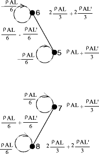

  

  Formation of the subgraph T

  $$ \mathrm{T}=\left[ {\begin{array}{cccccc} {\frac{{5\uprho \mathrm{A}\mathrm{L}}}{6}+\frac{{\uprho \mathrm{A}\mathrm{L}^{\prime}}}{3}} & {\frac{{\uprho \mathrm{A}\mathrm{L}}}{6}-\frac{{\uprho \mathrm{A}\mathrm{L}^{\prime}}}{6}} & 0 & 0 \\{\frac{{\uprho \mathrm{A}\mathrm{L}}}{6}-\frac{{\uprho \mathrm{A}\mathrm{L}^{\prime}}}{6}} & {\frac{{\uprho \mathrm{A}\mathrm{L}}}{2}+\frac{{2\uprho \mathrm{A}\mathrm{L}^{\prime}}}{3}} & 0 & 0 \\0 & 0 & {\frac{{7\uprho \mathrm{A}\mathrm{L}}}{6}+\frac{{\uprho \mathrm{A}\mathrm{L}^{\prime}}}{3}} & {\frac{{\uprho \mathrm{A}\mathrm{L}}}{6}+\frac{{\uprho \mathrm{A}\mathrm{L}^{\prime}}}{6}} \\0 & 0 & {\frac{{\uprho \mathrm{A}\mathrm{L}}}{6}+\frac{{\uprho \mathrm{A}\mathrm{L}^{\prime}}}{6}} & {\frac{{5\uprho \mathrm{A}\mathrm{L}}}{6}+\frac{{2\uprho \mathrm{A}\mathrm{L}^{\prime}}}{3}} \\\end{array}} \right]. $$

  (7.107)

Considering, $\mathrm{E}=2.07\times {10^7}\begin{array}{cccccc} \mathrm{{kN}/\mathrm{m}} \\\end{array}\mathrm{L}=100\mathrm{cm}$, $\mathrm{I}=100\begin{array}{cccccc} \mathrm{{c}{{\mathrm{m}}^2}} \\\end{array}$ and $\begin{array}{cccccc} {\uprho =78\begin{array}{cccccc} \mathrm{{kN}/{{\mathrm{m}}^3}} \\\end{array}} \\\end{array}$ and $\mathrm{A}=10\begin{array}{cccccc} \mathrm{{c}{{\mathrm{m}}^2}} \\\end{array}$ the frequencies of the structure are calculated as

$$ \openup 5pt\begin{array}{llll} {\omega_S} =[16.251,20.608,37.51,40.229] \hfill \\{\omega_T} =[8.294,42.680,45.403,55.909] \hfill \\\omega ={\omega_S}\cup {\omega_T}=[16.251,20.608,37.51,40.229,8.294,42.680,45.403,55.909]. \hfill \cr \end{array} $$

(7.108)

Using the algebraic approach formulated in Sect. 3.1, identical eigenfrequencies are obtained. The eigenvectors are then calculated and the mode shapes are obtained, Fig. 7.56.

Fig. 7.56

The natural mode shapes of Example 7.12

Example 7.13

Consider the symmetric truss with an even number of spans as shown in Fig. 7.57. For this truss, the axis of symmetry passes through two nodes.

Fig. 7.57

A truss with an even number of bays

The stiffness matrix of the structure shown in Fig. 7.58 has the Form B symmetry as follows:

Fig. 7.58

Graph representation of the stiffness matrix

$$ \mathbf{K} = \left[ {\begin{array}{*{20}{c}} {\frac{2\mathrm{EA}}{\mathrm{L}}+\frac{\mathrm{EA}}{{2\mathrm{L}^{\prime}}}} & 0 & {\frac{\mathrm{EA}}{{2\mathrm{L}^{\prime}}}} & 0 & 0 & 0 & 0 & 0 & {-\frac{\mathrm{EA}}{\mathrm{L}}} & {-\frac{\mathrm{EA}}{{2\mathrm{L}^{\prime}}}} & 0 & {-\frac{\mathrm{EA}}{{2\mathrm{L}^{\prime}}}} \\ 0 & {\frac{\mathrm{EA}}{\mathrm{L}}+\frac{\mathrm{EA}}{{{\mathrm{L}}^{\prime}}}} & 0 & 0 & 0 & 0 & 0 & 0 & {-\frac{\mathrm{EA}}{{2\mathrm{L}^{\prime}}}} & {-\frac{\mathrm{EA}}{\mathrm{L}}} & {\frac{\mathrm{EA}}{{2\mathrm{L}^{\prime}}}} & 0 \\ {\frac{\mathrm{EA}}{{2\mathrm{L}^{\prime}}}} & 0 & {\frac{\mathrm{EA}}{\mathrm{L}}+\frac{\mathrm{EA}}{{2\mathrm{L}^{\prime}}}} & {-\frac{\mathrm{EA}}{\mathrm{L}}} & 0 & 0 & 0 & 0 & 0 & {-\frac{\mathrm{EA}}{{2\mathrm{L}^{\prime}}}} & 0 & {-\frac{\mathrm{EA}}{{2\mathrm{L}^{\prime}}}} \\ 0 & 0 & {-\frac{\mathrm{EA}}{\mathrm{L}}} & {\frac{\mathrm{EA}}{\mathrm{L}}+\frac{\mathrm{EA}}{{{\mathrm{L}}^{\prime}}}} & 0 & 0 & 0 & 0 & {\frac{\mathrm{EA}}{{2\mathrm{L}^{\prime}}}} & 0 & {-\frac{\mathrm{EA}}{{2\mathrm{L}^{\prime}}}} & 0 \\ 0 & 0 & 0 & 0 & {\frac{2\mathrm{EA}}{\mathrm{L}}+\frac{\mathrm{EA}}{{2\mathrm{L}^{\prime}}}} & 0 & {-\frac{\mathrm{EA}}{{2\mathrm{L}^{\prime}}}} & 0 & {-\frac{\mathrm{EA}}{\mathrm{L}}} & {-\frac{\mathrm{EA}}{{2\mathrm{L}^{\prime}}}} & 0 & {\frac{\mathrm{EA}}{{2\mathrm{L}^{\prime}}}} \\ 0 & 0 & 0 & 0 & 0 & {\frac{\mathrm{EA}}{\mathrm{L}}+\frac{\mathrm{EA}}{{{\mathrm{L}}^{\prime}}}} & 0 & 0 & {-\frac{\mathrm{EA}}{{2\mathrm{L}^{\prime}}}} & {-\frac{\mathrm{EA}}{\mathrm{L}}} & {-\frac{\mathrm{EA}}{{2\mathrm{L}^{\prime}}}} & 0 \\ 0 & 0 & 0 & 0 & {-\frac{\mathrm{EA}}{{2\mathrm{L}^{\prime}}}} & 0 & {\frac{\mathrm{EA}}{\mathrm{L}}+\frac{\mathrm{EA}}{{2\mathrm{L}^{\prime}}}} & {-\frac{\mathrm{EA}}{\mathrm{L}}} & 0 & {\frac{\mathrm{EA}}{{2\mathrm{L}^{\prime}}}} & 0 & {-\frac{\mathrm{EA}}{{2\mathrm{L}^{\prime}}}} \\ 0 & 0 & 0 & 0 & 0 & 0 & {-\frac{\mathrm{EA}}{\mathrm{L}}} & {\frac{\mathrm{EA}}{\mathrm{L}}+\frac{\mathrm{EA}}{{{\mathrm{L}}^{\prime}}}} & {-\frac{\mathrm{EA}}{{2\mathrm{L}^{\prime}}}} & 0 & {-\frac{\mathrm{EA}}{{2\mathrm{L}^{\prime}}}} & 0 \\ {-\frac{\mathrm{EA}}{\mathrm{L}}} & {-\frac{\mathrm{EA}}{{2\mathrm{L}^{\prime}}}} & 0 & {\frac{\mathrm{EA}}{{2\mathrm{L}^{\prime}}}} & {-\frac{\mathrm{EA}}{\mathrm{L}}} & {-\frac{\mathrm{EA}}{{2\mathrm{L}^{\prime}}}} & 0 & {-\frac{\mathrm{EA}}{{2\mathrm{L}^{\prime}}}} & {\frac{2\mathrm{EA}}{\mathrm{L}}+\frac{\mathrm{EA}}{{{\mathrm{L}}^{\prime}}}} & 0 & 0 & 0 \\ {-\frac{\mathrm{EA}}{{2\mathrm{L}^{\prime}}}} & {-\frac{\mathrm{EA}}{\mathrm{L}}} & {-\frac{\mathrm{EA}}{{2\mathrm{L}^{\prime}}}} & 0 & {-\frac{\mathrm{EA}}{{2\mathrm{L}^{\prime}}}} & {-\frac{\mathrm{EA}}{\mathrm{L}}} & {\frac{\mathrm{EA}}{{2\mathrm{L}^{\prime}}}} & 0 & 0 & {\frac{2\mathrm{EA}}{\mathrm{L}}+\frac{\mathrm{EA}}{{{\mathrm{L}}^{\prime}}}} & 0 & 0 \\ 0 & {\frac{\mathrm{EA}}{{2\mathrm{L}^{\prime}}}} & 0 & {-\frac{\mathrm{EA}}{{2\mathrm{L}^{\prime}}}} & 0 & {-\frac{\mathrm{EA}}{{2\mathrm{L}^{\prime}}}} & 0 & {-\frac{\mathrm{EA}}{{2\mathrm{L}^{\prime}}}} & 0 & 0 & {\frac{\mathrm{EA}}{\mathrm{L}}+\frac{\mathrm{EA}}{{{\mathrm{L}}^{\prime}}}} & {-\frac{\mathrm{EA}}{\mathrm{L}}} \\ {-\frac{\mathrm{EA}}{{2\mathrm{L}^{\prime}}}} & 0 & {-\frac{\mathrm{EA}}{{2\mathrm{L}^{\prime}}}} & 0 & {\frac{\mathrm{EA}}{{2\mathrm{L}^{\prime}}}} & 0 & {-\frac{\mathrm{EA}}{{2\mathrm{L}^{\prime}}}} & 0 & 0 & 0 & {-\frac{\mathrm{EA}}{\mathrm{L}}} & {\frac{\mathrm{EA}}{\mathrm{L}}+\frac{\mathrm{EA}}{{{\mathrm{L}}^{\prime}}}} \\ \end{array}} \right]. $$

(7.109)

Graph representation of the stiffness matrix is illustrated in Fig. 7.58.

7.5.2.1 Symmetry Property of the Graph Representation of the Stiffness Matrix

• 1. The graph is symmetric with respect to the axis passing through the nodes corresponding to the central DOFs.

• 2. The weight of the node i is equal to the (i,i)th entry of the stiffness (or mass) matrix, and it is symmetric with respect to the axis.

• 3. The weight of the member connecting the nodes i and j is equal to the (i,j)th entry of the stiffness (or mass) matrix. The weight between the x DOFs (the upper part of the graph) and the weight of the member between y DOFs (lower part of the graph) are symmetric with respect to the axis of symmetry (the corresponding members are identical), and the weight of the members between x and y DOFs in two sides of the axis of symmetry is antisymmetric (equal members with reverse signs). Finally there should be no link member between x and y DOFs of the central nodes, that is, the submatrix L of the stiffness (or mass) matrices should be null matrix. This had been proven differently.

7.5.2.2 Formation of the Subgraphs

The subgraphs are constructed utilising the following algorithm:

We subdivide the graph into two subgraphs by removing the members cut by the axis of symmetry. The subgraph in the LHS corresponds to the matrix S, and the one in the RHS corresponds to T. For the graphs on the axis of symmetry, the upper nodes on the axis corresponding to the horizontal DOFs are associated to S and the bottom nodes on the axis corresponding to the vertical DOFs are associated to T. The weight of the nodes and all the members (which may exist between the nodes on the axis) are left unchanged.

• (a) The subgraph corresponding to S:

  If there exists a member between any node of the LHS (nodes 5, 6, 7 and 8) and the central nodes (the existing nodes in Figs. 7.57 and 7.58), then a directed member is added from the central node towards the node in the LHS with a weight equal to that of the existing member. The weight of the directed member from i to j is added to the entry S_ij.

  The stiffness matrix corresponding to the subgraph shown in Fig. 7.59 is constructed as

  Fig. 7.59

  

  Formation the subgraph S

  $$ {{\mathbf{K}}_{\mathrm{S}}}=\left[ {\begin{array}{*{20}{c}} {\frac{2\mathrm{EA}}{\mathrm{L}}+\frac{\mathrm{EA}}{{2\mathrm{L}^{\prime}}}} & 0 & {\frac{\mathrm{EA}}{{2\mathrm{L}^{\prime}}}} & 0 & {-\frac{\mathrm{EA}}{\mathrm{s}}} & {-\frac{\mathrm{EA}}{{2\mathrm{L}^{\prime}}}} \\ 0 & {\frac{\mathrm{EA}}{\mathrm{L}}+\frac{\mathrm{EA}}{{{\mathrm{L}}^{\prime}}}} & 0 & 0 & {-\frac{\mathrm{EA}}{{2\mathrm{L}^{\prime}}}} & {-\frac{\mathrm{EA}}{\mathrm{L}}} \\ {\frac{\mathrm{EA}}{{2\mathrm{L}^{\prime}}}} & 0 & {\frac{\mathrm{EA}}{\mathrm{L}}+\frac{\mathrm{EA}}{{2\mathrm{L}^{\prime}}}} & {-\frac{\mathrm{EA}}{\mathrm{L}}} & 0 & {-\frac{\mathrm{EA}}{{2\mathrm{L}^{\prime}}}} \\ 0 & 0 & {-\frac{\mathrm{EA}}{\mathrm{L}}} & {\frac{\mathrm{EA}}{\mathrm{L}}+\frac{\mathrm{EA}}{{{\mathrm{L}}^{\prime}}}} & {\frac{\mathrm{EA}}{{2\mathrm{L}^{\prime}}}} & 0 \\ {-\frac{2\mathrm{EA}}{\mathrm{L}}} & {-\frac{\mathrm{EA}}{{{\mathrm{L}}^{\prime}}}} & 0 & {-\frac{\mathrm{EA}}{{{\mathrm{L}}^{\prime}}}} & {\frac{2\mathrm{EA}}{\mathrm{L}}+\frac{\mathrm{EA}}{{{\mathrm{L}}^{\prime}}}} & 0 \\ {-\frac{\mathrm{EA}}{{{\mathrm{L}}^{\prime}}}} & {-\frac{2\mathrm{EA}}{\mathrm{L}}} & {-\frac{\mathrm{EA}}{{{\mathrm{L}}^{\prime}}}} & 0 & 0 & {\frac{2\mathrm{EA}}{\mathrm{L}}+\frac{\mathrm{EA}}{{{\mathrm{L}}^{\prime}}}} \\ \end{array}} \right]. $$

  (7.110)

• (b) The subgraph corresponding to T:

  The weight of the nodes and the possible existing members are left unchanged. If there exists a member between the DOFs of the RHS (nodes 5, 6, 7 and 8) and the central nodes (the existing nodes in Figs. 7.59 and 7.60), then another directed member is added from the LHS node towards the central node with a weight equal to that of the existing member. For the added directed member, the weight of the member from i to j is added to the entry T _ij.

  Fig. 7.60

  

  Formation the subgraph T

The stiffness matrix corresponding to the subgraph T, shown in Fig. 7.60, is constructed in the following:

$$ {K_T}=\left[ {\begin{array}{clclcllclcllclclcl}{\frac{2EA }{L}+\frac{EA }{{2{L}^{\prime}}}} & 0 & {-\frac{EA }{{2{L}^{\prime}}}} & 0 & 0 & {\frac{EA }{{L^{\prime}}}} & \\0 & {\frac{EA }{L}+\frac{EA }{{L^{\prime}}}} & 0 & 0 & {-\frac{EA }{{L^{\prime}}}} & 0 & \\{-\frac{EA }{{2{L}^{\prime}}}} & 0 & {\frac{EA }{L}+\frac{EA }{{2{L}^{\prime}}}} & {-\frac{EA }{L}} & 0 & {-\frac{EA }{{L^{\prime}}}} & \\0 & 0 & {-\frac{EA }{L}} & {\frac{EA }{L}+\frac{EA }{{L^{\prime}}}} & {-\frac{EA }{{L^{\prime}}}} & 0 & \\0 & {-\frac{EA }{{2{L}^{\prime}}}} & 0 & {-\frac{EA }{{2{L}^{\prime}}}} & {\frac{EA }{L}+\frac{EA }{{L^{\prime}}}} & {-\frac{EA }{L}} & \\{\frac{EA }{{2{L}^{\prime}}}} & 0 & {-\frac{EA }{{2{L}^{\prime}}}} & 0 & {-\frac{EA }{L}} & {\frac{EA }{L}+\frac{EA }{{L^{\prime}}}} & \\\end{array}} \right]. $$

(7.111)

For the mass matrix, a similar operation is performed.

$$ M=\left[ {\begin{array}{*{20}{c}} {\rho AL+\frac{{\rho A{L}^{\prime}}}{3}} & {\frac{{\rho AL}}{6}} & 0 & 0 & 0 & 0 & 0 & 0 & {\frac{{\rho AL}}{6}} & {\frac{{\rho A{L}^{\prime}}}{6}} & 0 & 0 \\ {\frac{{\rho AL}}{6}} & {\frac{{2\rho AL}}{3}+\frac{{2\rho A{L}^{\prime}}}{3}} & 0 & 0 & 0 & 0 & 0 & 0 & {\frac{{\rho A{L}^{\prime}}}{6}} & {\frac{{\rho AL}}{6}} & 0 & 0 \\ 0 & 0 & {\rho AL+\frac{{\rho A{L}^{\prime}}}{3}} & {\frac{{\rho AL}}{6}} & 0 & 0 & 0 & 0 & 0 & 0 & {\frac{{\rho AL}}{6}} & {\frac{{\rho A{L}^{\prime}}}{6}} \\ 0 & 0 & {\frac{{\rho AL}}{6}} & {\frac{{2\rho AL}}{3}+\frac{{2\rho A{L}^{\prime}}}{3}} & 0 & 0 & 0 & 0 & 0 & 0 & {\frac{{\rho A{L}^{\prime}}}{6}} & {\frac{{\rho AL}}{6}} \\ 0 & 0 & 0 & 0 & {\rho AL+\frac{{\rho A{L}^{\prime}}}{3}} & {\frac{{\rho AL}}{6}} & 0 & 0 & {\frac{{\rho AL}}{6}} & {\frac{{\rho A{L}^{\prime}}}{6}} & 0 & 0 \\ 0 & 0 & 0 & 0 & {\frac{{\rho AL}}{6}} & {\frac{{2\rho AL}}{3}+\frac{{2\rho A{L}^{\prime}}}{3}} & 0 & 0 & {\frac{{\rho A{L}^{\prime}}}{6}} & {\frac{{\rho AL}}{6}} & 0 & 0 \\ 0 & 0 & 0 & 0 & 0 & 0 & {\rho AL+\frac{{\rho A{L}^{\prime}}}{3}} & {\frac{{\rho AL}}{6}} & 0 & 0 & {\frac{{\rho AL}}{6}} & {\frac{{\rho A{L}^{\prime}}}{6}} \\ 0 & 0 & 0 & 0 & 0 & 0 & {\frac{{\rho AL}}{6}} & {\frac{{2\rho AL}}{3}+\frac{{2\rho A{L}^{\prime}}}{3}} & 0 & 0 & {\frac{{\rho A{L}^{\prime}}}{6}} & {\frac{{\rho AL}}{6}} \\ {\frac{{\rho AL}}{6}} & {\frac{{\rho A{L}^{\prime}}}{6}} & 0 & 0 & {\frac{{\rho AL}}{6}} & {\frac{{\rho A{L}^{\prime}}}{6}} & 0 & 0 & {\rho AL+\frac{{2\rho A{L}^{\prime}}}{3}} & {\frac{{\rho AL}}{6}} & 0 & 0 \\ {\frac{{\rho A{L}^{\prime}}}{6}} & {\frac{{\rho AL}}{6}} & 0 & 0 & {\frac{{\rho A{L}^{\prime}}}{6}} & {\frac{{\rho AL}}{6}} & 0 & 0 & {\frac{{\rho AL}}{6}} & {\rho AL+\frac{{2\rho A{L}^{\prime}}}{3}} & 0 & 0 \\ 0 & 0 & {\frac{{\rho AL}}{6}} & {\frac{{\rho A{L}^{\prime}}}{6}} & 0 & 0 & {\frac{{\rho AL}}{6}} & {\frac{{\rho A{L}^{\prime}}}{6}} & 0 & 0 & {AL+\frac{{2\rho A{L}^{\prime}}}{3}} & {\frac{{\rho AL}}{6}} \\ 0 & 0 & {\frac{{\rho A{L}^{\prime}}}{6}} & {\frac{{\rho AL}}{6}} & 0 & 0 & {\frac{{\rho A{L}^{\prime}}}{6}} & {\frac{{\rho AL}}{6}} & 0 & 0 & {\frac{{\rho AL}}{6}} & {\rho AL+\frac{{2\rho A{L}^{\prime}}}{3}} \\ \end{array}} \right]. $$

(7.112)

The graph representation of the mass matrix with the Form B symmetry is illustrated in Fig. 7.61.

Fig. 7.61

Graph representation of the mass matrix

The subgraphs are constructed utilising the previous algorithm.

• (a) The subgraph corresponding to S:

  The mass matrix corresponding to the subgraph, shown in Fig. 7.62, is formed as

  Fig. 7.62

  

  Formation of the subgraph S

  $$ {{\rm \bf M}_S}=\left[ {\begin{array}{cccccc} {\rho AL+\frac{{\rho A{L}^{\prime}}}{3}} & {\frac{{\rho AL}}{6}} & 0 & 0 & {\frac{{\rho AL}}{6}} & {\frac{{\rho A{L}^{\prime}}}{6}} \\{\frac{{\rho AL}}{6}} & {\frac{{2\rho AL}}{3}+\frac{{2\rho A{L}^{\prime}}}{3}} & 0 & 0 & {\frac{{\rho A{L}^{\prime}}}{6}} & {\frac{{\rho AL}}{6}} \\0 & 0 & {\rho AL+\frac{{\rho A{L}^{\prime}}}{3}} & {\frac{{\rho AL}}{6}} & 0 & 0 \\0 & 0 & {\frac{{\rho AL}}{6}} & {\frac{{2\rho AL}}{3}+\frac{{2\rho A{L}^{\prime}}}{3}} & 0 & 0 \\{\frac{{\rho AL}}{3}} & {\frac{{\rho A{L}^{\prime}}}{3}} & 0 & 0 & {\rho AL+\frac{{2\rho A{L}^{\prime}}}{3}} & {\frac{{\rho AL}}{6}} \\{\frac{{\rho A{L}^{\prime}}}{3}} & {\frac{{\rho AL}}{3}} & 0 & 0 & {\frac{{\rho AL}}{6}} & {\rho AL+\frac{{2\rho A{L}^{\prime}}}{3}} \\\end{array}} \right]. $$

  (7.113)

• (b) The subgraph corresponding to T:

  The mass matrix corresponding to the subgraph, shown in Fig. 7.63, is as follows:

  Fig. 7.63

  

  Formation of the subgraph T

  $$ {{\mathbf{M}}_\mathrm{{T}}}=\left[ {\begin{array}{cccccc} {\uprho \mathrm{A}\mathrm{L}+\frac{{\uprho \mathrm{A}\mathrm{L}^{\prime}}}{3}} & {\frac{{\uprho \mathrm{A}\mathrm{L}}}{6}} & 0 & 0 & 0 & 0 \\{\frac{{\uprho \mathrm{A}\mathrm{L}}}{6}} & {\frac{{2\uprho \mathrm{A}\mathrm{L}}}{3}+\frac{{2\uprho \mathrm{A}\mathrm{L}^{\prime}}}{3}} & 0 & 0 & 0 & 0 \\0 & 0 & {\uprho \mathrm{A}\mathrm{L}+\frac{{\uprho \mathrm{A}\mathrm{L}^{\prime}}}{3}} & {\frac{{\uprho \mathrm{A}\mathrm{L}}}{6}} & {\frac{{\uprho \mathrm{A}\mathrm{L}}}{3}} & {\frac{{\uprho \mathrm{A}\mathrm{L}^{\prime}}}{3}} \\0 & 0 & {\frac{{\uprho \mathrm{A}\mathrm{L}}}{6}} & {\frac{{2\uprho \mathrm{A}\mathrm{L}}}{3}+\frac{{2\uprho \mathrm{A}\mathrm{L}^{\prime}}}{3}} & {\frac{{\uprho \mathrm{A}\mathrm{L}^{\prime}}}{3}} & {\frac{{\uprho \mathrm{A}\mathrm{L}}}{3}} \\0 & 0 & {\frac{{\uprho \mathrm{A}\mathrm{L}}}{6}} & {\frac{{\uprho \mathrm{A}\mathrm{L}^{\prime}}}{6}} & {\uprho \mathrm{A}\mathrm{L}+\frac{{2\uprho \mathrm{A}\mathrm{L}^{\prime}}}{3}} & {\frac{{\uprho \mathrm{A}\mathrm{L}}}{6}} \\0 & 0 & {\frac{{\uprho \mathrm{A}\mathrm{L}^{\prime}}}{6}} & {\frac{{\uprho \mathrm{A}\mathrm{L}}}{6}} & {\frac{{\uprho \mathrm{A}\mathrm{L}}}{6}} & {\uprho \mathrm{A}\mathrm{L}+\frac{{2\uprho \mathrm{A}\mathrm{L}^{\prime}}}{3}} \\\end{array}} \right]. $$

  (7.114)

Considering $\mathrm{E}=2.07\times {10^7}\begin{array}{cccccc} \mathrm{{kN}/\mathrm{m}} \\\end{array}$, L = 100 cm, $\mathrm{I}=100\begin{array}{cccccc} \mathrm{{c}{{\mathrm{m}}^4}} \\\end{array}$ and $\begin{array}{cccccc} {\uprho =78\begin{array}{cccccc} \mathrm{{kN}/{{\mathrm{m}}^3}} \\\end{array}} \\\end{array}$ and, the frequencies of the structure are calculated as

$$ \begin{array}{llll} {\omega_T}=[48.908,42.227,37.548,31.368,26.525,5.447], \hfill \cr {\omega_S}=[11.886,14.184,11.722,42.890,45.349,59.192], \hfill \\ \omega ={\omega_T}\cup {\omega_S}=[48.908,42.227,37.548,31.368,26.525,5.447,11.886, \hfill \cr \qquad\qquad\qquad\quad14.184,11.722,42.890,45.349,59.192]. \hfill\end{array} $$

(7.115)

Using the algebraic approach formulated in Sect. 3.2, identical eigenfrequencies are obtained. The eigenvectors are then calculated and the mode shapes are obtained. The first four mode shapes are illustrated in Fig. 7.64.

Fig. 7.64

The first four natural mode shapes of Example 7.13

Important Notes: In the main graph there is no member between the nodes in the two sides of the symmetry axis, since the submatrices D, E and F are null matrices. The reason is the existence of a member directly connecting two nodes in two sides of the symmetry axis. If there exist such members, then the submatrices D, E and F will not be null, and for finding the subgraphs S and T and only for such members, one should act as was described in the algorithm for the Form B symmetry. For other members with the present pattern with nodes in two sides of the axis connected to the central node, the above algorithm should be employed. This problem can be recognised by investigating the similarity between the Form A and Form B canonical symmetries. Part of the matrices S and T in Form A are exactly the same as submatrices S and T in Form B.

Example 7.14

Consider a planar 2D truss with the symmetry axis passing through central members (truss with odd number of spans), as shown in Fig. 7.65.

Fig. 7.65

A 7-bay symmetric truss

Considering L = 100 cm, I = 100 cm⁴, E = 201 kN/mm² and $\uprho =78\mathrm{kN}/{{\mathrm{m}}^3}$, $A=10\mathrm{c}{{\mathrm{m}}^2}$, the eigenfrequencies of the structure are calculated as:

$$ \openup 4pt\begin{array}{llll} {\omega_S}=\left[{ \begin{array}{llll}26.83,42.78,92.36,108.31,150.23,159.69,169.32,171.32,180.91,\atop\cr 201.74,225.75,230.13,233.65,293.60\hfill\end{array}} \right], \hfill \cr {\omega_T}=\left[ {\begin{array}{llll} 11.40,58.91,76.81,122.52,140.75,174.27,177.88,183.17,217.99 ,\atop\cr 223.18,233.94,235.82,259.0,322.24 \hfill\end{array}} \right], \hfill \cr \omega ={\omega_S}\cup {\omega_T}=\left[ \openup -4.5pt{\begin{array}{cccccc} 26.83,42.78,92.36,108.31,150.23,159.69,169.32,171.32,180.91, \cr 201.74,225.75,230.13,233.65,293.60,11.40,58.91,76.81,122.52,\hfill \cr 140.75,174.27,177.88,183.17,217.99,223.18,233.94,235.82, \hfill\cr 259.0,322.24\hfill \end{array}} \right]\end{array} $$

(7.116)

Using the algebraic approach formulated in Sect. 3.1, identical eigenfrequencies are obtained.

Example 7.15

Consider a planar 2D trusses that passes symmetry axes on middle nodes (truss with even number of spans) as shown in Fig. 7.66.

Fig. 7.66

A 6-bay truss

Considering L = 100 cm, I = 100 cm⁴, E = 201 kN/mm² and $\uprho =78\mathrm{kN}/{{\mathrm{m}}^3}$, $A=10\mathrm{c}{{\mathrm{m}}^2}$, the eigenfrequencies of the structure are calculated as:

$$ \openup 4pt\begin{array}{llll} {\omega_K}=\left[{ \begin{array}{lllll} 319.33,247.61,32.86,50.60,235.05,226.08,210.38,111.94,119.87,162.88,\atop\cr 175.33,177.43\hfill\end{array}} \right], \hfill \cr {\omega_H}=\left[ {\begin{array}{llll} 15.17,73.08,86.37,142.5,157.8,170.21,182.37, 189.58,225.17,226.63\atop\cr 234.2,284.92 \hfill\end{array}} \right], \hfill \cr \omega ={\omega_K}\cup {\omega_H}=\left[ \openup -4.5pt{\begin{array}{cccccc} 319.33,247.61,32.86,50.60,235.05,226.08,210.38,111.94, \cr 119.87,162.88, 175.33,177.43,15.17,73.08,86.37,142.5,157.8,\hfill \cr 170.21,182.37,189.58,225.17 ,226.63,234.2,284.92\hfill \end{array}} \right]\end{array} $$

(7.117)

Using the algebraic approach formulated in Sect. 3.2, identical eigenfrequencies are obtained.

Though in this part the examples are selected from small trusses, however, the method shows its potential more when applied to large-scale structures. For comparison of the required time for calculating the eigenvalues of matrices with and without decomposition, matrices of various dimensions are considered having sparsity between 30 % and 40 %, and MATLAB is employed for these calculations.

7.5.3 Discussion

In this part two new canonical forms are introduced and weighted graph are associated with these forms. Decomposition and healing processes are presented to perform on these graphs in order to reduce the dimensions of the problem for free vibration analysis of the symmetric trusses. Therefore, the accuracy of calculation increases, and the cost of the computation decreases. The previously developed methods were unable to deal with cross-link members of structures with more than one DOF per node, while the new forms defined here overcome this difficulty. Calculation of the eigenfrequencies can also be performed using the relationships presented in Sects. 3.1 and 3.2 for trusses with odd and even numbers of bays, respectively.

It should be mentioned that for automatic numbering of the degrees of freedom (or nodal numbering suitable for the canonical forms), additional algorithm is required.

The present method is also applicable to similar eigensolution problems such as stability analysis of symmetric trusses for calculating their critical loads. This approach can easily be generalised to free vibration analysis of space trusses.

7.6 General Canonical Forms for Analytical Solution of Problems in Structural Mechanics

In this part new forms are introduced for efficient eigensolution of special tri-diagonal and penta-diagonal matrices. Applications of these forms are illustrated using problems from mechanics of structures.

7.6.1 Definitions

The polynomial $\mathrm{p}(\lambda ) = \det (\mathbf{A}-\lambda \mathbf{I})$ is called the characteristic polynomial of A. The roots of p(λ) = 0 are the eigenvalues of A. Since the degree of the characteristic polynomial p(λ) equals to N, the dimension of A has N roots, so A has N eigenvalues. A non-zero vector x satisfying $\mathbf{Ax}=\lambda \mathbf{x}$ is an eigenvector for the eigenvalue λ.

The easiest matrix for which the eigenvalues can be calculated is a diagonal matrix, whose eigenvalues are simply its diagonal entries. Equally easy is a triangular matrix, whose eigenvalues are also its diagonal entries. A matrix can have complex eigenvalues, since the roots of its characteristic polynomial may be real or complex. Therefore, there is not always a real triangular matrix with the same eigenvalues as a real general matrix, since a real triangular matrix can only have real eigenvalues. Thus, one must either use complex numbers or look beyond real triangular matrices for canonical forms for real matrices. For this purpose, it is sufficient to consider block triangular matrices, that is, matrices of the form

$$ \mathbf{A}=\left[ {\begin{array}{cccccc} {{{\mathbf{A}}_{11 }}} & {{{\mathbf{A}}_{12 }}} &. &. &. & {{{\mathbf{A}}_{{1\mathrm{N}}}}} \\{} & {{{\mathbf{A}}_{22 }}} &. &. &. & {{{\mathbf{A}}_{{2\mathrm{N}}}}} \\{} & {} &. &. &. &. \\{} & {} & {} &. &. &. \\{} & {} & {} & {} &. &. \\{} & {} & {} & {} & {} & {{{\mathbf{A}}_\mathrm{{NN}}}} \\\end{array}} \right], $$

(7.118)

where each A _ii is square and all entries below A _ii blocks are zero. It can easily be shown that the characteristic polynomial det (A − λ I) of A is the product $\prod\nolimits_{\mathrm{{i}=1}}^\mathrm{{N}} { \det } ({{\mathbf{A}}_\mathrm{{i}\mathrm{i}}}-\lambda \mathbf{I})$ of the characteristic polynomial of the A _ii, and therefore, the set λ(A) of eigenvalues of A is the union $\cup_{\mathrm{{i}=1}}^\mathrm{{N}}\lambda ({{\mathbf{A}}_\mathrm{{i}\mathrm{i}}})$ of the sets of eigenvalues of the diagonal blocks A _ii.

7.6.2 Decomposition of a Tri-diagonal Matrix

Consider a block tri-diagonal matrix as:

$$ \mathbf{F}=\left[ {\begin{array}{clclcllclcllclclcl}\mathbf{A} & \mathbf{B} & {} & {} & {} & {} & {} & {} & {} \\\mathbf{B} & \mathbf{C} & \mathbf{B} & {} & {} & {} & {} & {} & {} \\{} & \mathbf{B} & \mathbf{C} & \mathbf{B} & {} & {} & {} & {} & {} \\{} & {} &. &. &. & {} & {} & {} & {} \\{} & {} & {} &. &. &. & {} & {} & {} \\{} & {} & {} & {} &. &. &. & {} & {} \\{} & {} & {} & {} & {} & \mathbf{B} & \mathbf{C} & \mathbf{B} & {} \\{} & {} & {} & {} & {} & {} & \mathbf{B} & \mathbf{C} & \mathbf{B} \\{} & {} & {} & {} & {} & {} & {} & \mathbf{B} & \mathbf{A} \\\end{array}} \right], $$

(7.119)

where A, B and C are m × m matrix blocks. The matrix F contains n blocks in each row and n blocks in each column. A matrix M in the form of F will be denoted by ${{\mathbf{M}}_\mathrm{{m}\mathrm{n}}}=\mathbf{F}{{({{\mathbf{A}}_{\mathrm{m}}},{{\mathbf{B}}_{\mathrm{m}}},{{\mathbf{C}}_{\mathrm{m}}})}_\mathrm{{m}\mathrm{n}}}$.

7.6.2.1 Canonical Form I

Now consider the following tri-diagonal matrix:

$$ \begin{array}{cccccc} {{\mathbf{M}}_{\mathbf{m}\mathbf{n}}} = \mathbf{F}{{\left( {{{\mathbf{A}}_{\mathbf{m}}},\ {{\mathbf{B}}_{\mathbf{m}}},\ {{\mathbf{A}}_{\mathbf{m}}}} \right)}_{\mathbf{m}\mathbf{n}}}, \hfill \\ \mathrm{where}{{\mathbf{A}}_{\mathbf{m}}}=\mathbf{F}{{(\mathrm{a},\mathrm{b},\mathrm{a})}_{\mathbf{m}}}\mathbf{and}{{\mathbf{B}}_{\mathbf{m}}}=\mathbf{F}{{(\mathrm{c},\mathrm{d},\mathrm{c})}_{\mathbf{m}}}. \hfill\end{array} $$

(7.120)

Consider T _k = F(0,1,0)_k with eigenvalues λ _k, and denote the unit matrix by I _k, where k is the dimension of the square matrices T _k and I _k. The matrix M _mn can be decomposed as

$$ {{\mathbf{M}}_\mathrm{{m}\mathrm{n}}}={{\mathbf{I}}_\mathrm{{n}}}\otimes {{\mathbf{A}}_{\mathrm{m}}}+{{\mathbf{T}}_\mathrm{{n}}}\otimes {{\mathbf{B}}_{\mathrm{m}}}, $$

(7.121)

where ⊗ denotes the Kronecker product of two matrices as defined in Sect. 4.9. Substituting the following relationships in Eq. 7.121,

$$ {{\mathbf{A}}_{\mathrm{m}}}=\left( \mathrm{{a}{{\mathbf{I}}_{\mathrm{m}}}+\mathrm{b}{{\mathbf{T}}_{\mathrm{m}}}} \right)\kern0.75em \mathrm{and}\ {{\mathbf{B}}_{\mathrm{m}}}=\left( \mathrm{{c}{{\mathbf{I}}_{\mathrm{m}}}+\mathrm{d}{{\mathbf{T}}_{\mathrm{m}}}} \right) $$

(7.122)

results in

$$ {{\mathbf{M}}_\mathrm{{m}\mathrm{n}}}=\mathrm{a}{{\mathbf{I}}_\mathrm{{n}}}\otimes {{\mathbf{I}}_{\mathrm{m}}}+\mathrm{b}{{\mathbf{I}}_\mathrm{{n}}}\otimes {{\mathbf{T}}_{\mathrm{m}}}+\mathrm{c}{{\mathbf{T}}_\mathrm{{n}}}\otimes {{\mathbf{I}}_{\mathrm{m}}}+\mathrm{d}{{\mathbf{T}}_\mathrm{{n}}}\otimes {{\mathbf{T}}_{\mathrm{m}}}. $$

(7.123)

It is readily verified that the eigenvalues of ${{\mathbf{T}}_\mathrm{{n}}}\otimes {{\mathbf{T}}_{\mathrm{m}}}$ are λ _m λ _n, and therefore,

$$ \lambda = \mathrm{a} + \mathrm{b}{\lambda_{\mathrm{m}}} + \mathrm{c}{\lambda_\mathrm{{n}}} + \mathrm{d}{\lambda_{\mathrm{m}}}{\lambda_\mathrm{{n}}}. $$

(7.124)

7.6.2.2 Applications

For problems where the second derivatives are present, the application of finite difference method leads to matrices of canonical Form I. As an example, consider the solution of the Laplace equation using the finite difference method. The parameters of λ in Eq. 7.124 for this case are as follows:

$$ \mathrm{a} = 4,\ \mathrm{b} = -1,\ \mathrm{c} = -1,\ \mathrm{a}\mathrm{nd}\ \mathrm{d} = 0, $$

(7.125)

leading to

$$ \lambda = 4-{\lambda_{\mathrm{m}}}-{\lambda_\mathrm{{n}}}. $$

(7.126)

Now consider the solution of the Laplace equation in a square domain, Fig. 7.50, with N = 4 (m = n = 4).

In general case, for a path P_n with n nodes, the adjacency and Laplacian matrices are in the form P_n = F(a,b,a), and the corresponding eigenvalues can be obtained by (Fig. 7.67)

Fig. 7.67

A square domain and its grid points

$$ \lambda =\mathrm{a} + 2\mathrm{b} \cos \frac{\mathrm{{k}\uppi}}{\mathrm{{n}+1}}\mathrm{for}\ \mathrm{k}=1,\ldots,\mathrm{n}. $$

(7.127)

For T _m = F(0,1,0) one obtains ${\lambda_{\mathrm{m}}}=2 \cos \frac{\mathrm{{k}\uppi}}{\mathrm{{n}+1}}$, and for maximum, ${\lambda_4}=2 \cos \frac{\uppi}{5}=1.6180$, leading to λ = 4 − 1.6180 − 1.6180 = 0.7639 which is quite close to the exact value. Figures 7.68a and 7.69b show the distribution of the components of the corresponding first eigenvector, over the grid points, in two- and three-dimensional spaces, respectively.

Fig. 7.68

Distributions of the first eigenvector in 2D and 3D spaces. (a) Components of the first eigenvector in 2D space. (b) Components of the first eigenvector in 3D space

Fig. 7.69

A symmetric frame with sway

7.6.3 A New Form for Efficient Solution of Eigenproblem

7.6.3.1 A General Block Diagonal Tri-diagonal Matrix

Consider a block tri-diagonal matrix as

$$ \mathbf{M}=\left[ {\begin{array}{clclcllclcllclclcl}\mathrm{x} & 3 &{\vrule height 8pt depth 4pt} & 0 & 2 &{\vrule height 8pt depth 4pt} & 0 & 0 \cr\noalign{} 4 & \mathrm{x} &{\vrule height 8pt depth 4pt} & \mathrm{x} & 0 &{\vrule height 8pt depth 4pt} & 0 & 0 \cr\noalign{} \noalign{\hrule} 0 & 2 &{\vrule height 8pt depth 4pt} & \mathrm{x} & 3 &{\vrule height 8pt depth 4pt} & 0 & 2 \cr\noalign{} \mathrm{x} & 0 &{\vrule height 8pt depth 4pt} & 4 & \mathrm{x} &{\vrule height 8pt depth 4pt} & \mathrm{x} & 0 \cr\noalign{} \noalign{\hrule} 0 & 0 &{\vrule height 8pt depth 4pt} & 0 & 2 &{\vrule height 8pt depth 4pt} & \mathrm{x} & 3 \cr\noalign{} 0 & 0 &{\vrule height 8pt depth 4pt} & \mathrm{x} & 0 &{\vrule height 8pt depth 4pt} & 4 & \mathrm{x} \\\end{array}} \right] $$

(7.128)

with x as some diagonal and non-diagonal entries. We are interested to find x such that the determinant of M becomes zero. This matrix has the canonical Form I as introduced in the previous section, and it can be expressed as P _m = F(A ₂,B ₂,A ₂). The corresponding eigenvalues can be obtained as

$$ \lambda ={{\mathbf{A}}_2}+2{{\mathbf{B}}_2} \cos \frac{\mathrm{{k}\uppi}}{\mathrm{{n}+1}};\ \mathrm{k}=1,\ldots,\mathrm{n}. $$

(7.129)

Now one can substitute the corresponding submatrices for A ₂ and B ₂, leading to

$$ \lambda =\left[ {\begin{array}{cccccc} \mathrm{x} & 3 \\4 & \mathrm{x} \\\end{array}} \right]+2\left[ {\begin{array}{cccccc} 0 & 2 \\\mathrm{x} & 0 \\\end{array}} \right] \cos \frac{\mathrm{{k}\uppi}}{4};\ \mathrm{k}=1,\ldots,3. $$

(7.130)

For det (M) = 0, the determinant of ${\lambda_{\mathbf{M}}}$ for k = 1,2,3 should be set to zero, that is,

$$ \begin{array}{cccccc} \det \left( {\left[ {\begin{array}{cccccc} \mathrm{x} & 3 \\4 & \mathrm{x} \\\end{array}} \right]+2\left[ {\begin{array}{cccccc} 0 & 2 \\\mathrm{x} & 0 \\\end{array}} \right] \cos \frac{\uppi}{4}} \right)=0\Rightarrow \mathrm{x}=10.4695,\kern0.5em \mathrm{x}=-2.2268, \hfill \\\det \left( {\left[ {\begin{array}{cccccc} \mathrm{x} & 3 \\4 & \mathrm{x} \\\end{array}} \right]+2\left[ {\begin{array}{cccccc} 0 & 2 \\\mathrm{x} & 0 \\\end{array}} \right] \cos \frac{{2\uppi}}{4}} \right)=0\Rightarrow \mathrm{x}=3.4641,\kern0.5em \mathrm{x}=-3.4641, \hfill \\\det \left( {\left[ {\begin{array}{cccccc} \mathrm{x} & 3 \\4 & \mathrm{x} \\\end{array}} \right]+2\left[ {\begin{array}{cccccc} 0 & 2 \\\mathrm{x} & 0 \\\end{array}} \right] \cos \frac{{3\uppi}}{4}} \right)=0\Rightarrow \mathrm{x}=0.7159,\kern0.5em \mathrm{x}=-0.9586. \hfill\end{array} $$

(7.131)

These are exactly the same eigenvalues obtained from det (M) = 0.

For the special case $\mathrm{n}=2$, we have

$$ \mathbf{M}=\left[ {\begin{array}{cccccc} \mathbf{A} & \mathbf{B} \\\mathbf{B} & \mathbf{A} \\\end{array}} \right], $$

(7.132)

resulting in

$$ \begin{array}{*{20}{c}} { \det \left( {\mathbf{A}+2 \cos \frac{\uppi}{3}\mathbf{B}} \right)=0} \\ { \det \left( {\mathbf{A}\hbox{-}2 \cos \frac{\uppi}{3}\mathbf{B}} \right)=0} \\ \end{array}\Rightarrow\,\,\,\begin{array}{*{20}{c}} { \det (\mathbf{A}+\mathbf{B})=0} \\ { \det (\mathbf{A}-\mathbf{B})=0} \\ \end{array}. $$

(7.133)

In general, one can write

$$ \det (\mathbf{M})=0\kern0.5em \Rightarrow \det \left( {\mathbf{A}+2 \cos \frac{\mathrm{{k}\uppi}}{\mathrm{{n}+1}}\mathbf{B}} \right)=0\kern0.5em \mathrm{for}\ \mathrm{i}=1,2,\ldots,\mathrm{n}. $$

(7.134)

Example 7.16

Consider the symmetric frame as shown in Fig. 7.69. The numbering for DOFs is chosen that a Form II symmetry is provided for the structural matrices. For all the members, EI is taken as ‘a’ and the unit length mass is assumed to be 10 kg/m.

The stiffness and mass matrices are formed as

$$ \begin{array}{cccccc} \mathbf{K}=\mathrm{a}\openup7pt\left[ {\begin{array}{cccccc} {\displaystyle\frac{284 }{105 }} & {\displaystyle\frac{2}{3}} &{\vrule height 14pt depth 9pt} & {\displaystyle\frac{2}{7}} & 0 \cr\noalign{} \displaystyle{\frac{2}{3}} & {\displaystyle\frac{40 }{21 }} &{\vrule height 14pt depth 12pt} & 0 & {\displaystyle\frac{2}{7}} \cr\noalign{} \noalign{\hrule} {\displaystyle\frac{2}{7}} & 0 &{\vrule height 17pt depth 17pt} & {\displaystyle\frac{284 }{105 }} & {\displaystyle\frac{2}{3}} \cr\noalign{} 0 & {\displaystyle\frac{2}{7}} &{\vrule height 14pt depth 7pt} & {\displaystyle\frac{2}{3}} & {\displaystyle\frac{40 }{21 }} \\\end{array}} \right]\mathrm{and}\cr \mathbf{M}=\openup3pt\left[ {\begin{array}{cccccc} {\displaystyle\frac{990 }{21 }} & {\displaystyle\frac{-81 }{42 }} &{\vrule height 10pt depth 17pt} & {\displaystyle\frac{-1029 }{42 }} & 0 \cr\noalign{} {\displaystyle\frac{-81 }{42 }} & {\displaystyle\frac{740 }{21 }} &{\vrule height 10pt depth 14pt} & 0 & {\displaystyle\frac{-1029 }{42 }} \cr\noalign{} \noalign{\hrule} {\displaystyle\frac{-1029 }{42 }} & 0 &{\vrule height 17pt depth 14pt} & {\displaystyle\frac{990 }{21 }} & {\displaystyle\frac{-81 }{42 }} \cr\noalign{} 0 & {\displaystyle\frac{-1029 }{42 }} &{\vrule height 10pt depth 7pt} & {\displaystyle\frac{-81 }{42 }} & {\displaystyle\frac{740 }{21 }} \\\end{array}} \right].\end{array} $$

(7.135)

The matrix $\left[ {\mathbf{K}-{\omega^2}\mathbf{M}} \right]$ has a Form II pattern, Eq. 7.132, and using Eq. 7.133, we have

$$ \begin{array}{cccccc} \det \left[ {\begin{array}{cccccc} {2.41-71.6\mathrm{x}} & {0.67+2\mathrm{x}} \\{0.67+2\mathrm{x}} & {1.61-59.7\mathrm{x}} \\\end{array}} \right]=0 \hfill \\\det \left[ {\begin{array}{cccccc} {2.99-22.6\mathrm{x}} & {0.67+2\mathrm{x}} \\{0.67+2\mathrm{x}} & {2.19-10.7\mathrm{x}} \\\end{array}} \right]=0 \hfill\end{array} $$

(7.136)

where $\mathrm{x}=\frac{{{\omega^2}}}{\mathrm{{a}}}$, leading to the following natural frequencies:

$$ \begin{array}{cccccc} {{\mathrm{{x}}_1}=0.019\Rightarrow \omega_1^2=0.019\mathrm{a}} & {{\mathrm{{x}}_3}=0.102\Rightarrow \omega_3^2=0.102\mathrm{a},} \\{{\mathrm{{x}}_2}=0.042\Rightarrow \omega_2^2=0.042\mathrm{a}} & {{\mathrm{{x}}_4}=0.252\Rightarrow \omega_4^2=0.252\mathrm{a}.} \\\end{array} $$

(7.137)

Example 7.17

Consider a one-span frame as shown in Fig. 7.70. The columns are subdivided into two elements. Therefore, the frame has six DOFs as illustrated in the figure. The stiffness matrix of the structure is assembled as follows:

Fig. 7.70

A portal frame with six DOF

$$ \begin{array}{clclcllclcllclclcl}\mathbf{K}=\frac{\mathrm{EI}}{{{{\mathrm L}^3}}}\left[ {\begin{array}{clclcllclcllclclcl}{192} & 0 & {-48} &{\vrule height 8pt depth 4pt} & 0 & 0 & 0 \cr\noalign{} 0 & {64} & {16} &{\vrule height 8pt depth 4pt} & 0 & 0 & 0 \cr\noalign{} {-48} & {16} & {36} &{\vrule height 8pt depth 4pt} & 0 & 0 & 2 \cr\noalign{} \noalign{\hrule} 0 & 0 & 0 &{\vrule height 8pt depth 4pt} & {192} & 0 & {-48} \cr\noalign{} 0 & 0 & 0 &{\vrule height 8pt depth 4pt} & 0 & {64} & {16} \cr\noalign{} 0 & 0 & 2 &{\vrule height 8pt depth 4pt} & {-48} & {16} & {36} \\\end{array}} \right]\ \hfill \cr\noalign{} \kern8.5em -\frac{\mathrm P}{\mathrm L}\left[ {\begin{array}{clclcllclcllclclcl}{\frac{24 }{5}} & 0 & {\frac{-1 }{5}} &{\vrule height 10pt depth 6pt} & 0 & 0 & 0 \cr\noalign{} 0 & {\frac{8}{15 }} & {\frac{-1 }{15 }} &{\vrule height 10pt depth 6pt} & 0 & 0 & 0 \cr\noalign{} {\frac{-1 }{5}} & {\frac{-1 }{15 }} & {\frac{4}{15 }} &{\vrule height 10pt depth 7pt} & 0 & 0 & 0 \cr\noalign{} \noalign{\hrule} 0 & 0 & 0 &{\vrule height 10pt depth 6pt} & {\frac{24 }{5}} & 0 & {\frac{-1 }{5}} \cr\noalign{} 0 & 0 & 0 &{\vrule height 10pt depth 6pt} & 0 & {\frac{8}{15 }} & {\frac{-1 }{15 }} \cr\noalign{} 0 & 0 & 0 &{\vrule height 10pt depth 6pt} & {\frac{-1 }{5}} & {\frac{-1 }{15 }} & {\frac{4}{15 }} \\\end{array}} \right]. \hfill\end{array} $$

(7.138)

This matrix has Form II and the smallest eigenvalue corresponds to ${\mathrm{{P}}_\mathrm{{cr}}}=\frac{{22.2097\mathrm{EI}}}{{{\mathrm{{L}}^2}}}$. This is an approximate value compared to the real value as ${\mathrm{{P}}_\mathrm{{cr}}}=\frac{{25.2\mathrm{EI}}}{{{\mathrm{{L}}^2}}}.$ A better result can be obtained by subdividing the columns into three elements and the beam into two elements.

Example 7.18

Consider a one-bay two-storey frame as shown in Fig. 7.71a. This example is studied with two different discretisations. In the first model, each column is considered as one element as in Fig. 7.71a, and in the second model, each column is subdivided into two elements as illustrated in Fig. 7.4.

Fig. 7.71

A one-bay two-storey frame. (a) Four degrees of freedom. (b) Fourteen degrees of freedom

For the first model ${\mathrm{{P}}_\mathrm{{cr}}}=\frac{{19.75\mathrm{EI}}}{{{\mathrm{{L}}^2}}}$, which is a crude answer.

For the second model shown in Fig. 7.71b, the stiffness matrix is formed as

$$ \begin{gathered} \mathbf{K}=\frac{\mathrm{EI}}{{{{\mathrm{L}}^3}}}\left[ {\begin{array}{*{20}{c}} {192} & 0 & {-48} & 0 & 0 & 0 &\vline & 0 & 0 & 0 & 0 & 0 & 0 \\ 0 & {64} & {16} & 0 & 0 & 0 &\vline & 0 & 0 & 0 & 0 & 0 & 0 \\ {-48} & {16} & {36} & 0 & 0 & 0 &\vline & 0 & 0 & 2 & 0 & 0 & 0 \\ 0 & 0 & 0 & {192} & 0 & {-48} &\vline & 0 & 0 & 0 & 0 & 0 & 0 \\ 0 & 0 & 0 & 0 & {64} & {16} &\vline & 0 & 0 & 0 & 0 & 0 & 0 \\ 0 & 0 & 0 & {-48} & {16} & {36} &\vline & 0 & 0 & 0 & 0 & 0 & 2 \\ \hline 0 & 0 & 0 & 0 & 0 & 0 &\vline & {192} & 0 & {-48} & 0 & 0 & 0 \\ 0 & 0 & 0 & 0 & 0 & 0 &\vline & 0 & {64} & {16} & 0 & 0 & 0 \\ 0 & 0 & 2 & 0 & 0 & 0 &\vline & {-48} & {12} & {36} & 0 & 0 & 0 \\ 0 & 0 & 0 & 0 & 0 & 0 &\vline & 0 & 0 & 0 & {192} & 0 & {-48} \\ 0 & 0 & 0 & 0 & 0 & 0 &\vline & 0 & 0 & 0 & 0 & {64} & {16} \\ 0 & 0 & 0 & 0 & 0 & 2 &\vline & 0 & 0 & 0 & {-48} & {16} & {36} \\ \end{array}} \right] \hfill \\ -\frac{\mathrm{P}}{\mathrm{L}}\left[ {\begin{array}{*{20}{c}} {\frac{48 }{5}} & 0 & {\frac{-2 }{5}} & 0 & 0 & 0 &\vline & 0 & 0 & 0 & 0 & 0 & 0 \\ 0 & {\frac{16 }{15 }} & {\frac{-2 }{15 }} & 0 & 0 & 0 &\vline & 0 & 0 & 0 & 0 & 0 & 0 \\ {\frac{-2 }{5}} & {\frac{-2 }{15 }} & {\frac{8}{15 }} & 0 & 0 & 0 &\vline & 0 & 0 & 0 & 0 & 0 & 0 \\ 0 & 0 & 0 & {\frac{24 }{5}} & 0 & {\frac{-1 }{5}} &\vline & 0 & 0 & 0 & 0 & 0 & 0 \\ 0 & 0 & 0 & 0 & {\frac{8}{5}} & {\frac{-1 }{15 }} &\vline & 0 & 0 & 0 & 0 & 0 & 0 \\ 0 & 0 & 0 & {\frac{-1 }{5}} & {\frac{-1 }{15 }} & {\frac{4}{15 }} &\vline & 0 & 0 & 0 & 0 & 0 & 0 \\ \hline 0 & 0 & 0 & 0 & 0 & 0 &\vline & {\frac{48 }{5}} & 0 & {\frac{-2 }{5}} & 0 & 0 & 0 \\ 0 & 0 & 0 & 0 & 0 & 0 &\vline & 0 & {\frac{16 }{15 }} & {\frac{-2 }{15 }} & 0 & 0 & 0 \\ 0 & 0 & 0 & 0 & 0 & 0 &\vline & {\frac{-2 }{5}} & {\frac{-2 }{15 }} & {\frac{8}{15 }} & 0 & 0 & 0 \\ 0 & 0 & 0 & 0 & 0 & 0 &\vline & 0 & 0 & 0 & {\frac{24 }{5}} & 0 & {\frac{-1 }{5}} \\ 0 & 0 & 0 & 0 & 0 & 0 &\vline & 0 & 0 & 0 & 0 & {\frac{8}{15 }} & {\frac{-1 }{15 }} \\ 0 & 0 & 0 & 0 & 0 & 0 &\vline & 0 & 0 & 0 & {\frac{-1 }{5}} & {\frac{-1 }{15 }} & {\frac{4}{15 }} \\ \end{array}} \right] \hfill \\ \end{gathered} $$

(7.139)

leading to ${\mathrm{{P}}_\mathrm{{cr}}}=\frac{{11.1049\mathrm{EI}}}{{{\mathrm{{L}}^2}}}$. Subdividing the columns into three elements and the beams into two elements leads to ${\mathrm{{P}}_\mathrm{{cr}}}=\frac{{12.7554\mathrm{EI}}}{{{\mathrm{{L}}^2}}}$. The exact value for the critical load is ${\mathrm{{P}}_{\mathrm{{cr}(\mathrm{exact})}}}=\frac{{12.60\mathrm{EI}}}{{{\mathrm{{L}}^2}}}$.

7.6.4 Canonical Penta-diagonal Form

7.6.4.1 Formulation

The numerical solution of some problems results in five-diagonal matrices. An example of this form is depicted in the following:

$$ {{\mathbf{M}}_\mathrm{{mn}}}={{\left[ {\begin{array}{clclcllclcllclclcl}\mathbf{A} & \mathbf{B} & \mathbf{I} & {} & {} & {} & {} & {} & {} \\\mathbf{B} & {\mathbf{A}+\mathbf{I}} & \mathbf{B} & \mathbf{I} & {} & {} & {} & {} & {} \\\mathbf{I} & \mathbf{B} & {\mathbf{A}+\mathbf{I}} &. &. & {} & {} & {} & {} \\{} &. &. &. &. &. & {} & {} & {} \\{} & {} &. &. &. &. &. & {} & {} \\{} & {} & {} &. &. &. &. &. & {} \\{} & {} & {} & {} &. &. &. & \mathbf{B} & \mathbf{I} \\{} & {} & {} & {} & {} &. & \mathbf{B} & {\mathbf{A}+\mathbf{I}} & \mathbf{B} \\{} & {} & {} & {} & {} & {} & \mathbf{I} & \mathbf{B} & \mathbf{A} \\\end{array}} \right]}_{\mathrm{{n}\times \mathrm{n}}}}. $$

(7.140)

Using the Kronecker product, this matrix can be decomposed as

$$ {{\mathbf{M}}_\mathrm{{m}\mathrm{n}}}={{\mathbf{I}}_\mathrm{{n}}}\otimes {{\mathbf{A}}_{\mathrm{m}}}+{{\mathbf{T}}_\mathrm{{n}}}\otimes {{\mathbf{B}}_{\mathrm{m}}}+{{\mathbf{S}}_\mathrm{{n}}}\otimes {{\mathbf{I}}_{\mathrm{m}}} $$

(7.141)

where

$$ {{\mathbf{T}}_\mathrm{{n}}}=\mathbf{F}(0,1,0)\mathrm{and}{{\mathbf{S}}_\mathrm{{n}}}=\left[ {\begin{array}{cccccc} 0 & 0 & 1 & {} & {} & {} \\0 & 1 & 0 & 1 & {} & {} \\1 & 0 & 1 &. &. & {} \\{} & 1 &. &. &. &. \\{} & {} &. &. &. &. \\{} & {} & {} &. &. &. \\\end{array}} \right]. $$

(7.142)

It can easily be verified that

$$ {{\mathbf{S}}_\mathrm{{n}}}=\mathbf{T}_\mathrm{{n}}^2-{{\mathbf{I}}_\mathrm{{n}}}. $$

(7.143)

Therefore,

$$ \begin{array}{cccccc} {{\mathbf{M}}_\mathrm{{m}\mathrm{n}}} ={{\mathbf{I}}_\mathrm{{n}}}\otimes {{\mathbf{A}}_{\mathrm{m}}}+{{\mathbf{T}}_\mathrm{{n}}}\otimes {{\mathbf{B}}_{\mathrm{m}}}+\left( {\mathbf{T}_\mathrm{{n}}^2-{{\mathbf{I}}_\mathrm{{n}}}} \right)\otimes {{\mathbf{I}}_{\mathrm{m}}} \hfill \\\kern2.5em = {{\mathbf{I}}_\mathrm{{n}}}\otimes \left( {{{\mathbf{A}}_{\mathrm{m}}}-{{\mathbf{I}}_{\mathrm{m}}}} \right)+{{\mathbf{T}}_\mathrm{{n}}}\otimes {{\mathbf{B}}_{\mathrm{m}}}+\mathbf{T}_\mathrm{{n}}^2\otimes {{\mathbf{I}}_{\mathrm{m}}}. \hfill\end{array} $$

(7.144)

In the last two terms, T _n cannot be factorised, since we have a matrix product and not a Kronecker product. Therefore, the eigenvalues of the last two terms are calculated to search for a possible equivalent matrix with the same eigenvalues:

$$ {\lambda_{{{{\mathbf{T}}_\mathrm{{n}}}\otimes {{\mathbf{B}}_{\mathrm{m}}}+\mathbf{T}_\mathrm{{n}}^2\otimes {{\mathbf{I}}_{\mathrm{m}}}}}}={{\mathbf{B}}_{\mathrm{m}}}{\lambda_{{{{\mathbf{T}}_\mathrm{{n}}}}}}+{{\mathbf{I}}_{\mathrm{m}}}{\lambda_{{\mathbf{T}_\mathrm{{n}}^2}}}. $$

(7.145)

On the other hand, we have

$$ {\lambda_{{\mathbf{T}_\mathrm{{n}}^2}}}={{\left( {{\uplambda_{{{{\mathbf{T}}_\mathrm{{n}}}}}}} \right)}^2} $$

(7.146)

Hence,

$$ {\lambda_{{{{\mathbf{T}}_\mathrm{{n}}}\otimes {{\mathbf{B}}_{\mathrm{m}}}+\mathbf{T}_\mathrm{{n}}^2\otimes {{\mathbf{I}}_{\mathrm{m}}}}}}={\lambda_{{{{\mathbf{T}}_\mathrm{{n}}}}}}\left( {{{\mathbf{B}}_{\mathrm{m}}}+{\lambda_{{{{\mathbf{T}}_\mathrm{{n}}}}}}{{\mathbf{I}}_{\mathrm{m}}}} \right)={\lambda_{{{{\mathbf{T}}_\mathrm{{n}}}}}}\left( {{{\mathbf{B}}_{\mathrm{m}}}+2{{\mathbf{I}}_{\mathrm{m}}} \cos \frac{\mathrm{{k}\uppi}}{\mathrm{{n}+1}}} \right). $$

(7.147)

This is the same as the eigenvalue of the following matrix:

$$ {{\mathbf{T}}_\mathrm{{n}}}\otimes \left( {{{\mathbf{B}}_{\mathrm{m}}}+2{{\mathbf{I}}_{\mathrm{m}}} \cos \frac{\mathrm{{k}\uppi}}{\mathrm{{n}+1}}} \right). $$

(7.148)

Substituting in Eq. 7.144 leads to

$$ \begin{array}{cccccc} {{\mathbf{M}}_\mathrm{{m}\mathrm{n}}} ={{\mathbf{I}}_\mathrm{{n}}}\otimes \left( {{{\mathbf{A}}_{\mathrm{m}}}-{{\mathbf{I}}_{\mathrm{m}}}} \right)+{{\mathbf{T}}_\mathrm{{n}}}\otimes {{\mathbf{B}}_{\mathrm{m}}}+\left( {\mathbf{T}_\mathrm{{n}}^2\otimes {{\mathbf{I}}_{\mathrm{m}}}} \right) \hfill \\\kern2.5em ={{\mathbf{I}}_\mathrm{{n}}}\otimes \left( {{{\mathbf{A}}_{\mathrm{m}}}-{{\mathbf{I}}_{\mathrm{m}}}} \right)+{{\mathbf{T}}_\mathrm{{n}}}\otimes \left( {{{\mathbf{B}}_{\mathrm{m}}}+2{{\mathbf{I}}_{\mathrm{m}}}\cos \frac{\mathrm{{k}\uppi}}{\mathrm{{n}+1}}} \right). \hfill\end{array} $$

(7.149)

It can be seen that we have again a canonical Form I expressed as

$$ \mathbf{F}\left( {{{\mathbf{A}}_{\mathrm{m}}}-{{\mathbf{I}}_{\mathrm{m}}},{{\mathbf{B}}_{\mathrm{m}}}\left( {2{{\mathbf{I}}_{\mathrm{m}}}\cos \frac{\mathrm{{k}\uppi}}{\mathrm{{n}+1}}} \right),{{\mathbf{A}}_{\mathrm{m}}}-{{\mathbf{I}}_{\mathrm{m}}}} \right) $$

(7.150)

and the eigenvalues of this form should be calculated. Therefore, a five-diagonal form is transformed to a tri-diagonal form, and

$$ \begin{array}{cccccc} {\lambda_{\mathbf{M}}} =\left( {{{\mathbf{A}}_{\mathrm{m}}}-{{\mathbf{I}}_{\mathrm{m}}}} \right)+2\cos \frac{\mathrm{{k}\uppi}}{\mathrm{{n}+1}}\left( {{{\mathbf{B}}_{\mathrm{m}}}+2{{\mathbf{I}}_{\mathrm{m}}}\left( {\cos \frac{\mathrm{{k}\uppi}}{\mathrm{{n}+1}}} \right)} \right) \hfill \\ ={{\mathbf{A}}_{\mathrm{m}}}+2{{\mathbf{B}}_{\mathrm{m}}}\cos \frac{\mathrm{{k}\uppi}}{\mathrm{{n}+1}}+{{\mathbf{I}}_{\mathrm{m}}}\left( {4\cos^2 \frac{\mathrm{{k}\uppi}}{\mathrm{{n}+1}}-1} \right) \hfill \\ ={{\mathbf{A}}_{\mathrm{m}}}+2{{\mathbf{B}}_{\mathrm{m}}}\cos \frac{\mathrm{{k}\uppi}}{\mathrm{{n}+1}}+{{\mathbf{I}}_{\mathrm{m}}}\left( {1+2\cos \frac{{2\mathrm{k}\uppi}}{\mathrm{{n}+1}}} \right). \hfill\end{array} $$

(7.151)

Example 7.19

Consider a simply supported square thin plate as shown in Fig. 7.72. The buckling load of this plate under uniform compressive loads N_x = N_y = N is required. The governing differential equation of the plate is

$$ \frac{{{\partial^4}\mathrm{w}}}{{\partial {{\mathrm{x}}^4}}}+2\frac{{{\partial^4}\mathrm{w}}}{{\partial {{\mathrm{x}}^2}{{\mathrm{y}}^2}}}+\frac{{{\partial^4}\mathrm{w}}}{{\partial {{\mathrm{y}}^4}}}+\frac{\mathrm{N}}{\mathrm{D}}\left( {\frac{{{\partial^2}\mathrm{w}}}{{\partial {{\mathrm{x}}^2}}}+\frac{{{\partial^2}\mathrm{w}}}{{\partial {{\mathrm{y}}^2}}}} \right)=0, $$

(7.152)

or

Fig. 7.72

A plate under biaxial compressive loading

$$ {\nabla^4}\mathrm{w}+\frac{\mathrm{N}}{\mathrm{D}}{\nabla^2}\mathrm{w}=0. $$

(7.153)

The exact solution of this problem is as follows:

$$ {\mathrm{{N}}_\mathrm{{cr}}}=\frac{{2{\uppi^2}\mathrm{D}}}{{{\mathrm{{a}}^2}}}=\frac{{19.7392\mathrm{D}}}{{{\mathrm{{a}}^2}}}. $$

(7.154)

Using the finite difference method leads to a five-diagonal matrix with the pattern studied in the previous section. In a special case, when n = 6 (i.e. each edge is divided into six segments), the final form of M and the matrices A _m and B _m are as follows:

$$ {{\mathbf{A}}_5}={{\mathbf{F}}_5}(18-4\upalpha, \upalpha -8,19-4\upalpha ),{{\mathbf{B}}_5}={{\mathbf{F}}_5}(\upalpha -8,2,\,\upalpha -8),\ \mathrm{with}\,\upalpha =\frac{{\mathrm{N}{{{\left( {\frac{\mathrm{a}}{6}} \right)}}^2}}}{\mathrm{D}}=\frac{{\mathrm{N}{{\mathrm{a}}^2}}}{{36\mathrm{D}}}. $$

(7.155)

Therefore, det (M) = 0 leads to

$$ {\lambda_{\mathbf{M}}}={{\mathbf{A}}_5}+2{{\mathbf{B}}_5} \cos \frac{\mathrm{{k}\uppi}}{6}+{{\mathbf{I}}_5}\left( {1+2 \cos \frac{{2\mathrm{k}\uppi}}{6}} \right)=0\kern0.5em \mathrm{for}\ \mathrm{k}=1,2,\ldots,5. $$

(7.156)

Thus, instead of the matrix M with different magnitudes of k, the smallest value for k = 1 should be calculated, the main aim being the calculation of the critical load. This reduces the dimension of the matrix from 25 × 25 to 5 × 5. The latter matrix can itself be reduced as

For k = 1,

$$ \begin{gathered} {\lambda_{\mathbf{M}}}=\mathbf{F}(\mathrm{a},\,\mathrm{b},\,\mathrm{c})= \hfill \\ \mathbf{F}\left( {8-4\upalpha +2\left( { \cos \frac{\uppi}{6}} \right)(\upalpha -8)+1+2\, \cos \frac{{2\uppi}}{6},\upalpha -8+4\, \cos \frac{\uppi}{6},19-4\upalpha +2\left( { \cos \frac{\uppi}{6}} \right)(\upalpha -8)+1+2\cos \frac{{2\uppi}}{6}} \right). \hfill \\ \end{gathered} $$

(7.157)

Here c = a + 1, that is this matrix has a similar form to that of the five-diagonal matrix (7.22). Therefore, for calculating the eigenvalues, one can again employ the same relationship, leading to

$$ {\lambda_{{{\lambda_{\mathbf{M}}}}}}=0\Rightarrow \mathbf{A}+2\mathbf{B} \cos \frac{\mathrm{{k}^{\prime}\uppi}}{\mathrm{{n}+1}}+\mathbf{I}\left( {1+2\cos \frac{{2\mathrm{k}^{\prime}\uppi}}{\mathrm{{n}+1}}} \right)=0\kern0.5em. $$

(7.158)

For k′ = 1, we have

$$\begin{array}{cccccc} 18-4\upalpha +2\left( { \cos \frac{\uppi}{6}} \right)(\upalpha -8)+1+2 \cos \frac{{2\uppi}}{6}+2 \cos \frac{\uppi}{6}\left( {\upalpha -8+4\cos \frac{\uppi}{6}} \right)\\ + \mathrm{I}\left( {1+2 \cos \frac{{2\uppi}}{6}} \right)=0 \end{array}$$

(7.159)

with I being a 1 × 1 unit matrix. Therefore, the 5 × 5 matrix is further reduced to a 1 × 1 matrix, that is, one equation with one unknown. Thus,

$$ \upalpha =\frac{{6-8 \cos \frac{\uppi}{6}+2 \cos \frac{{2\uppi}}{6}}}{{1 - \cos \frac{\uppi}{6}}}=0.5359\Rightarrow \frac{{{\mathrm{{N}}_\mathrm{{cr}}}{\mathrm{{a}}^2}}}{{36\mathrm{D}}}=\upalpha \Rightarrow {\mathrm{{N}}_\mathrm{{cr}}}=\frac{{19.2923\mathrm{D}}}{{{\mathrm{{a}}^2}}}. $$

(7.160)

7.6.4.2 Derivation of the Exact Solution

Having α in terms of the parameter n, the exact value of α can also be derived as follows:

$$ {\upalpha_{\mathrm{ext}}}=\mathop{\mathrm{Limit}}\limits_{{\mathrm{n}\to \infty }}\frac{{6-8 \cos \frac{\uppi}{\mathrm{n}}+2 \cos \frac{{2\uppi}}{\mathrm{n}}}}{{1- \cos \frac{\uppi}{\mathrm{n}}}}. $$

(7.161)

Using cos 2θ = 2cos²θ − 1 leads to

$$ {\upalpha_{\mathrm{ext}}}=\mathop{\mathrm{Limit}}\limits_{{\mathrm{n}\to \infty }}\frac{{4{{{\left( {1- \cos \frac{\uppi}{\mathrm{n}}} \right)}}^2}}}{{1- \cos \frac{\uppi}{\mathrm{n}}}}=\mathop{\mathrm{Limit}}\limits_{{\mathrm{n}\to \infty }}\ 4\left( {1- \cos \frac{\uppi}{\mathrm{n}}} \right). $$

(7.162)

Employing the following trigonometric relation and approximating sin θ by θ, if θ → 0, then we have

$$ 1- \cos\uptheta =2\mathbf{si}{{\mathbf{n}}^2}\frac{\uptheta}{2}\approx 2{{\left( {\frac{\uptheta}{2}} \right)}^2}=\frac{{{\uptheta^2}}}{2}. $$

(7.163)

Therefore,

$$ {\upalpha_\mathrm{{ext}}}=4\frac{{{{{(\uppi )}}^2}}}{{2{\mathrm{{n}}^2}}}=\frac{{2{\uppi^2}}}{{{\mathrm{{n}}^2}}}. $$

(7.164)

Substituting for α, we have

$$ \frac{{{{\mathrm{N}}_{\mathrm{cr}}}{{{\left( {\frac{\mathrm{a}}{\mathrm{n}}} \right)}}^2}}}{\mathrm{D}}=\frac{{2{\uppi^2}}}{{{{\mathrm{n}}^2}}}, $$

(7.165)

leading to the exact value of the critical load

$$ {{\left( {{\mathrm{{N}}_\mathrm{{cr}}}} \right)}_\mathrm{{ext}}}=\frac{{2\mathrm{D}{\uppi^2}}}{{{\mathrm{{a}}^2}}}=\frac{{19.7392\mathrm{D}}}{{{\mathrm{{a}}^2}}}. $$

(7.166)

7.7 Numerical Examples for the Matrices as the Sum of Three Kronecker Products

Matrices that can be written as the sum of three Kronecker products are already introduced in Sects. 4.10 and 4.11. In this part, examples are included to show the efficiency of this decomposition approach.

In this section, five examples are presented from structural mechanics to illustrate the applicability and the efficiency of the present methods.

Example 7.20

Consider the truss shown in Fig. 7.73. The cross-sectional areas and the mass of the members are as follows:

Fig. 7.73

A simple planar truss

Member	Cross-sectional area	Mass
1 and 2	A	m
3	1.5 A	3 m
4 and 5	1.5 A	2 m

The natural frequencies of the structure are required.

Using the finite element approach, the stiffness and mass matrices for a typical element are as follows:

$$ \left[ {{{\mathbf{K}}_\mathrm{{i}}}} \right]=\frac{\mathrm{{E}{\mathrm{{A}}_\mathrm{{i}}}}}{{{\mathrm{{h}}_\mathrm{{i}}}}}\left[ {\begin{array}{cccccc} {{\mathrm{{C}}^2}} & \mathrm{{C}\mathrm{S}} & {-{\mathrm{{C}}^2}} & {-\mathrm{CS}} \\\mathrm{{C}\mathrm{S}} & {{\mathrm{{S}}^2}} & {-\mathrm{CS}} & {-{\mathrm{{S}}^2}} \\{-{\mathrm{{C}}^2}} & {-\mathrm{CS}} & {{\mathrm{{C}}^2}} & \mathrm{{C}\mathrm{S}} \\{-\mathrm{CS}} & {-{\mathrm{{S}}^2}} & \mathrm{{C}\mathrm{S}} & {{\mathrm{{S}}^2}} \\\end{array}} \right],\ \left[ {{{\mathbf{M}}_\mathrm{{i}}}} \right]=\frac{{{{\mathrm{m}}_\mathrm{{i}}}{\mathrm{{h}}_\mathrm{{i}}}}}{6}\left[ {\begin{array}{cccccc} 2 & 0 & 1 & 0 \\0 & 2 & 0 & 1 \\1 & 0 & 2 & 0 \\0 & 1 & 0 & 2 \\\end{array}} \right], $$

where C = cos θ and S = sin θ.

After assembling the matrices of the elements for the entire structure and deleting the rows and columns corresponding to support nodes 1 and 2, we obtain

$$ \begin{gathered} [\mathbf{K}]=\frac{\mathrm{EA}}{{16\sqrt{3}\mathrm{L}}}\left[ {\begin{array}{*{20}{c}} {32.9090} & {-9} & 0 & 0 \\ {-9} & {39.5885} & 0 & {-24} \\ 0 & 0 & {32.9090} & 9 \\ 0 & {-24} & 9 & {39.5885} \\ \end{array}} \right],\kern0.5em \hfill \\ {}[\mathbf{M}]=\frac{\mathrm{mL}}{{16\sqrt{3}}}\left[ {\begin{array}{*{20}{c}} {31.3960} & 0 & 8 & 0 \\ 0 & {31.3960} & 0 & 8 \\ 8 & 0 & {31.3960} & 0 \\ 0 & 8 & 0 & {31.3960} \\ \end{array}} \right].\det \left( {\mathbf{K}-\mathbf{M}{\upomega^2}} \right)=0. \hfill \\ \end{gathered} $$

It can be observed that K and M have no particular form as modelled; however, one can multiply a row and the corresponding column in (−1) such that the eigenvalues remain unchanged. If such operations are performed for the first row and column of K and the corresponding M, then we obtain a Form II matrix, and constructing M + N and M − N, the eigenvalues can be obtained as

$$ \upomega =\{0.5614,\ 0.8887,\ 1.2195,\ 1.6624\}\times \sqrt{{\frac{\mathrm{EA}}{{\mathrm{m}{{\mathrm{L}}^2}}}}}. $$

Example 7.21

Using three finite elements we want to find the natural frequencies of the clamped beam shown in Fig. 7.74. The stiffness and mass matrices of a typical element are as follows:

Fig. 7.74

A clamped beam with three elements

$$ \begin{array}{cccccc} \left[ {{{\mathbf{K}}_\mathrm{{i}}}} \right]=\frac{\mathrm{{E}{\mathrm{{I}}_\mathrm{{i}}}}}{\mathrm{{L}_\mathrm{{i}}^3}}\left[ {\begin{array}{cccccc} {12} & {6\mathrm{L}} & {-12} & {6\mathrm{L}} \\{6\mathrm{L}} & {4{\mathrm{{L}}^2}} & {-6\mathrm{L}} & {2{\mathrm{{L}}^2}} \\{-12} & {-6\mathrm{L}} & {12} & {-6\mathrm{L}} \\{6\mathrm{L}} & {2{\mathrm{{L}}^2}} & {-6\mathrm{L}} & {4{\mathrm{{L}}^2}} \\\end{array}} \right], \hfill \cr \left[ {{{\mathbf{M}}_\mathrm{{i}}}} \right]=\frac{{{\uprho_\mathrm{{i}}}{\mathrm{{A}}_\mathrm{{i}}}{\mathrm{{L}}_\mathrm{{i}}}}}{420}\left[ {\begin{array}{cccccc} {156} & {22\mathrm{L}} & {54} & {-13\mathrm{L}} \\{22\mathrm{L}} & {4{\mathrm{{L}}^2}} & {13\mathrm{L}} & {-3{\mathrm{{L}}^2}} \\{54} & {13\mathrm{L}} & {156} & {-22\mathrm{L}} \\{-13\mathrm{L}} & {-3{\mathrm{{L}}^2}} & {-22\mathrm{L}} & {4{\mathrm{{L}}^2}} \\\end{array}} \right]. \hfill\end{array} $$

Assembling the matrices for the entire structure and applying the boundary conditions, the equation of vibration is as follows:

$$ \frac{{\uprho \mathrm{AL}}}{420}\left[ {\begin{array}{*{20}{c}} {312} & 0 & {54} & {-13\mathrm{L}} \\ 0 & {8{{\mathrm{L}}^2}} & {13\mathrm{L}} & {-3{{\mathrm{L}}^2}} \\ {54} & {13\mathrm{L}} & {312} & 0 \\ {-13\mathrm{L}} & {-3{{\mathrm{L}}^2}} & 0 & {8{{\mathrm{L}}^2}} \\ \end{array}} \right]\left[ {\begin{array}{*{20}{c}} {{{{\ddot{\mathrm{U}}}}_1}} \\ {{{{\ddot{\mathrm{U}}}}_2}} \\ {{{{\ddot{\mathrm{U}}}}_3}} \\ {{{{\ddot{\mathrm{U}}}}_4}} \\ \end{array}} \right] + \frac{\mathrm{EI}}{{{{\mathrm{L}}^3}}}\left[ {\begin{array}{*{20}{c}} {24} & 0 & {-12} & {6\mathrm{L}} \\ 0 & {8{{\mathrm{L}}^2}} & {-6\mathrm{L}} & {2{{\operatorname{L}}^2}} \\ {-12} & {-6\mathrm{L}} & {24} & 0 \\ {6\mathrm{L}} & {2{{\mathrm{L}}^2}} & 0 & {8{{\mathrm{L}}^2}} \\ \end{array}} \right]\left[ {\begin{array}{*{20}{c}} {{{\mathrm{U}}_1}} \\ {{{\mathrm{U}}_2}} \\ {{{\mathrm{U}}_3}} \\ {{{\mathrm{U}}_4}} \\ \end{array}} \right]=\left[ {\begin{array}{*{20}{c}} 0 \\ 0 \\ 0 \\ 0 \\ \end{array}} \right] $$

Here again one cannot see Form II matrices. However, multiplying the first row and column by (−1), such matrices can be constructed. Using their factors, similar to Example 7.20, the eigenvalues are obtained as

$$ \omega =\{2.4961,6.9893,16.2561,32.3059\}\times \sqrt{{\frac{\mathrm{{EI}}}{{\rho \mathrm{A}{\mathrm{{L}}^4}}}}}. $$

Example 7.22

Consider a simply supported a$\times$a square plate, as shown in Fig. 7.75. The load is applied in x-direction. Using the finite difference approach, the critical load of the plate is calculated.

Fig. 7.75

A simply supported plate

Considering the governing differential equation as

$$ {\nabla^4}\mathrm{w}+\frac{{{{\mathrm{N}}_{\mathrm{x}}}}}{\mathrm{D}}\ \frac{{{\partial^2}\mathrm{w}}}{{\partial {{\mathrm{x}}^2}}}=0 $$

and employing the finite difference method, the matrix M is obtained in the following form:

$$ \mathbf{M}=\mathbf{I}\otimes \mathbf{A}+\mathbf{T}\otimes \mathbf{B}+\mathbf{S}\otimes \mathbf{I}=\sum\limits_{\mathrm{{i}=1}}^3 {{{\mathbf{A}}_\mathrm{{i}}}\otimes {{\mathbf{B}}_\mathrm{{i}}}} $$

where

$$ \begin{array}{cccccc} {{\mathbf{B}}_1}=\mathbf{F}(18-2\mathrm{x},\mathrm{x}-8,19-2\mathrm{x},1),\;{{\mathbf{B}}_2}=\mathbf{F}(-8,2,-8),\ \cr {{\mathbf{A}}_2}=\mathbf{F}(0,1,0),{{\mathbf{A}}_3}=\mathbf{F}(0,0,1,1).\end{array} $$

Since ${{\mathbf{A}}_\mathrm{{i}}}{{\mathbf{A}}_\mathrm{{j}}}={{\mathbf{A}}_\mathrm{{j}}}{{\mathbf{A}}_\mathrm{{i}}}$ for each pair of i and j, then

$$ \begin{array}{llll} {\lambda_{\mathbf{M}}}=\mathop{\cup}\limits_{\mathrm{{j}=1}}^\mathrm{{n}}\left[ \mathrm{{eig}\sum\limits_{\mathrm{{i}=1}}^3 {{\lambda_\mathrm{{j}}}\left( {{{\mathbf{A}}_\mathrm{{i}}}} \right){{\mathbf{B}}_\mathrm{{i}}})} } \right]; {\lambda_{{{{\mathbf{A}}_1}}}}=1,\ {\lambda_{{{{\mathbf{A}}_2}}}}=2 \cos \frac{\mathrm{{k}\uppi}}{\mathrm{{n}+1}},\ \\ {\lambda_{{{{\mathbf{A}}_3}}}}=1+2 \cos \frac{{2\mathrm{k}\uppi}}{\mathrm{{n}+1}}. \end{array}$$

Once ${\lambda_{\mathbf{M}}}$ is calculated, it can be observed that it contains diagonal blocks and each block has the Form F. Thus, the diagonalisation is performed once again for each block, since ${{\mathbf{A}}_\mathrm{{i}}}{{\mathbf{A}}_\mathrm{{j}}}={{\mathbf{A}}_\mathrm{{j}}}{{\mathbf{A}}_\mathrm{{i}}}$ still holds for these blocks.

For critical load (k = 1), we have

$$\begin{array}{cccccc}18- 2\mathrm{x}-16 \cos \frac{\uppi}{\mathrm{m}}+1+2 \cos \frac{{2\uppi}}{\mathrm{m}}+2 \cos \frac{\uppi}{\mathrm{m}}\left( \mathrm{{x}-8+4 \cos \frac{\uppi}{\mathrm{m}}} \right)\cr +1\left( {1+2 \cos \frac{{2\uppi}}{\mathrm{m}}} \right)=0;\ \mathrm{m}=\mathrm{n}+1\end{array}$$

$$\Rightarrow \mathrm{x}=\frac{{4\left( {3-4 \cos \displaystyle\frac{\uppi}{\mathrm{m}}+ \cos \frac{{2\uppi}}{\mathrm{m}}} \right)}}{{\left( {1- \cos \displaystyle\frac{\uppi}{\mathrm{m}}} \right)}}.$$

In this relationship, $\rm m\to \infty$ leads to an accurate value of the critical load as $\mathrm{x}=\displaystyle\frac{{4{\uppi^2}}}{{{{\mathrm{m}}^2}}}$, where $1- \cos\upalpha \cong \displaystyle\frac{{{\upalpha^2}}}{2}\kern0.5em$ when $\upalpha \to 0$. This result is in a good agreement with the exact value, which is

$$ {{\mathrm{N}}_{\mathrm{cr}}}=\frac{\mathrm{xD}}{{{{{\left( {\frac{\mathrm{a}}{\mathrm{m}}} \right)}}^2}}} = \frac{{4{\uppi^2}\mathrm{D}}}{{{{\mathrm{a}}^2}}}. $$

Example 7.23

In the previous example, suppose the supports with no loading are clamped, then the matrix M will still contain the decomposability property. In such a case,

$$ \mathbf{A}=\mathbf{F}(20-2\mathrm{x},-8,19-2\mathrm{x},1),\kern0.75em \mathbf{B}=\mathbf{F}(\mathrm{x}-8,2,\mathrm{x}-8). $$

Using Eq. 7.171, M appears in a block form and the block corresponding to k = 1 is

$$ \begin{array}{cccccc} \mathbf{N}=\mathbf{F}\left( {20-2\mathrm{x}+2 \cos \frac{\uppi}{\mathrm{m}}(\mathrm{x}-8)+1+2 \cos \frac{{2\uppi}}{\mathrm{m}},\kern0.5em -8+4 \cos \frac{\uppi}{\mathrm{m}},} \right. \hfill \\\kern1.75em \left. {19-2\mathrm{x}+2 \cos \frac{\uppi}{\mathrm{m}}(\mathrm{x}-8)+1+2 \cos \frac{{2\uppi}}{\mathrm{m}},1} \right);\kern0.75em \mathrm{m}=\mathrm{n}+1 \hfill\end{array} $$

$$ {{\mathbf{A}}_1}=\mathbf{F}(0,1,0,0),\kern0.75em {{\mathbf{A}}_2}=\mathbf{F}(0,0,-1,1). $$

Here, unlike the previous case, N does not satisfy ${{\mathbf{A}}_\mathrm{{i}}}{{\mathbf{A}}_\mathrm{{j}}}={{\mathbf{A}}_\mathrm{{j}}}{{\mathbf{A}}_\mathrm{{i}}}$ and no further simplification is possible. Thus, one should form det (N) = 0 and solve it. Assuming n = 8, this solution leads to

$$ \mathrm{x}=1.1073\to {\mathrm{{N}}_\mathrm{{cr}}}=7.1804\frac{{{\uppi^2}\mathrm{D}}}{{{\mathrm{{a}}^2}}}. $$

The exact value of the critical load is ${\mathrm{{N}}_\mathrm{{cr}}}=7.69\displaystyle\frac{{{\uppi^2}\mathrm{D}}}{{{\mathrm{{a}}^2}}}$. Here, in place of the determinant of a 49 × 49 matrix, that of a 7 × 7 matrix is calculated. Choosing larger values for n, one can easily increase the accuracy of the finite difference approach. The present method reduces the size of a matrix to its square root. It should be added that for a rectangular plate when subdivided into equal lengths in x- and y-directions, similar forms will be formed.

Example 7.24

The natural bending and axial frequencies of the beam shown in Fig. 7.76 is required.

Fig. 7.76

A simple beam and its discretisation

The differential equation governing the bending of this beam can be written as

$$ \frac{{{{\mathrm{d}}^4}\mathrm{w}}}{{\mathrm{d}{{\mathrm{x}}^4}}}-{\upbeta^4}\mathrm{w}=0\ \,\mathrm{where}\ \,\upbeta =\frac{{\uprho \mathrm{A}{\upomega^2}}}{\mathrm{EI}}. $$

Choosing n + 1 element for discretisation of the beam, the final matrix becomes an n × n matrix in the following form:

$$ \mathbf{M}=\mathbf{F}(5,-4,6,1),=5\mathbf{I}+(-4)\mathbf{T}+\mathbf{S} $$

where T, S and I commute two by two, and therefore, Eq. 7.171 can be employed leading to

$$ \begin{array}{cccccc} {\lambda_{\mathbf{M}}} =5-8 \cos \upalpha +(1+2 \cos 2\upalpha )=6-8 \cos \upalpha +2 \cos 2\upalpha =4{{\left( {1- \cos \upalpha} \right)}^2}\cr =16\mathrm{si}{\mathrm{{n}}^4}\frac{\upalpha}{2} \cr \upalpha =\frac{\mathrm{{k}\uppi}}{\mathrm{m}};\kern0.75em \mathrm{m}=\mathrm{n}+1. \hfill\end{array} $$

On the other hand,

$$ {\omega_\mathrm{{k}}}=\left( {\upbeta \mathrm{L}} \right)_\mathrm{{k}}^2\sqrt{{\frac{\mathrm{{EI}}}{\mathrm{{m}{\mathrm{{L}}^4}}}}}\ \ \ \left( {\upbeta \mathrm{L}} \right)_\mathrm{{k}}^2={{\left( \mathrm{{n}+1} \right)}^2}\sqrt{\lambda}=4{{\mathrm{m}}^2}\mathrm{si}{\mathrm{{n}}^2}\frac{\upalpha}{2} $$

leading to the exact answer as

$$ \mathrm{n}\to \infty \Rightarrow \left( {\upbeta \mathrm{L}} \right)_\mathrm{{k}}^2=4{{\mathrm{m}}^2}\frac{{{\mathrm{{k}}^2}{\uppi^2}}}{{4{{\mathrm{m}}^2}}}\Rightarrow {{\left( {\upbeta \mathrm{L}} \right)}_\mathrm{{k}}}=\mathrm{k}\uppi \Rightarrow {\omega_\mathrm{{k}}}={{\left( \mathrm{{k}\uppi} \right)}^2}\sqrt{{\frac{\mathrm{{EI}}}{\mathrm{{m}{\mathrm{{L}}^4}}}}}\kern0.5em \mathrm{k}=1:\mathrm{n}. $$

For the axial vibration, the governing equation is as follows:

$$ \frac{{{\mathrm{{d}}^2}\mathrm{U}}}{\mathrm{{d}{\mathrm{{x}}^2}}}+{\upalpha^2}\mathrm{U}=0 $$

where

$$ \upalpha =\frac{{\uprho {\upomega^2}}}{\mathrm{E}}. $$

In this case, the matrix corresponding to the finite difference will be a tri-diagonal matrix as M = F(2,−1,2), and we have the following results:

$$ \mathbf{M}=2\mathbf{I}+(-1)\mathbf{T}\Rightarrow {\lambda_{\mathbf{M}}}=2+(-1)(2 \cos \upalpha )=4\mathrm{si}{\mathrm{{n}}^2}\frac{\upalpha}{2}, $$

$$ {\upomega_{\mathrm{k}}}={\upbeta_{\mathrm{k}}}\sqrt{{\frac{\mathrm{EA}}{\mathrm{m}}}}\ \ \ {{\left( {\upbeta \mathrm{L}} \right)}_{\mathrm{k}}}=(\mathrm{n}+1)\sqrt{\uplambda}=2\mathrm{m} \sin \frac{\upalpha}{2}, $$

$$ \mathrm{n}\to \infty \Rightarrow {{\left( {\upbeta \mathrm{L}} \right)}_{\mathrm{k}}}=2\mathrm{m}\frac{{\mathrm{k}\uppi}}{{2\mathrm{m}}}=\mathrm{k}\uppi \Rightarrow {\upomega_{\mathrm{k}}}=\frac{{\mathrm{k}\uppi}}{\mathrm{L}}\sqrt{{\frac{\mathrm{EA}}{\mathrm{m}}}}. $$

This is an exact answer. For a beam with clamped support, a similar approach leads to the exact result.

7.8 Symmetric Finite Element Formulation Using Canonical Forms: Truss and Frame Elements

In this part, canonical forms are used to decompose the symmetric line elements (truss and beam elements) into sub-elements of less the number of degrees of freedom (DOFs). Then the matrices associated with each sub-element are formed, and finally the matrices associated with each subsystem are combined to form the matrices of the prime element. Therefore, it becomes possible to find the pros and cons of this method and compare the efficiency and simplicity of the present approach to the existing methods.

7.8.1 Sign Convention

In this section, for computation of fundamental matrices for symmetric finite elements, the origin of the local coordinate system of the elements is taken at the centre of symmetry of the elements. Therefore, the symmetry axis or symmetry plane of each element will divide it into two parts: the positive half and the negative half.

If the symmetry axis passes through a node, that node will be numbered as node 1. Otherwise, node number 1 is usually chosen on the positive side of the element. Then, all of the nodes on the positive side are numbered sequentially. Having the nodes on the positive half of the element labelled, say from 1 (or 2) up to k, the rest of the nodes (nodes on the negative half of the element) must be numbered, considering the nodes of the positive side. This means that numbering of the negative side should be started with the node which is associated with the permutation of the first positive node, and is numbered as k + 1. Then, the reflection of the second positive node is labelled as k + 2, and this process is continued. The numbering process is terminated with the negative node which is permutation of the last positive node. Degrees of freedom (DOFs) of each node are numbered following the same rule.

Translation in positive direction and counterclockwise rotation for a positive node (node in the positive part of the element) define the positive translational and rotational DOFs for such nodes. Positive directions for negative nodes are selected such that the DOFs for a node and its reflection are the mirror of each other. For the node which is located at the centre of symmetry (if available), the positive directions can be selected arbitrarily. Figure 7.77 shows two one-dimensional (line) elements and numbering of the nodes and associated positive degrees of freedom, based on the convention described above.

Fig. 7.77

Numbering of the nodes and the DOFs for symmetric line elements. (a) Two-node truss element. (b) Two-node beam element. (c) Three-node beam element. (d) Five-node beam element

For two- or three-dimensional elements, the general approach for numbering and defining the positive directions are the same. If an element has more than one plane of symmetry, in order to apply the strategy described above, first, one of the planes should be selected as the main plane, and then during the numbering process for positive points (and DOFs), other planes of symmetry are taken into account one by one. Figure 7.78 shows the numbering and positive DOFs for a plane element possessing two main planes of symmetry: 1–1 and 2–2, where plane 1–1 which is in bold, has been taken as the principal symmetry plane. The node in the positive–positive quarter has been selected as node 1, its image with respect to plane 2–2 is labelled as node 2 and then the negative nodes have been numbered with respect to the principal plane of symmetry (1–1). It should be noted that as soon as the positive DOFs for node 1 are fixed, the positive direction for the other DOFs will be determined by means of symmetry properties.

Fig. 7.78

Numbering of the nodes and DOFs for symmetric plane elements

7.8.2 Truss Element

In this section, the properties of special symmetry form of the truss element shown in Fig. 7.77a are utilised in order to decompose the space of variables of this element into subspaces of divisor and co-divisor. This decreases the size of matrices and vectors which are involved in formulation of such element and therefore leads to a reduction in calculation time and computational effort.

Although such a reduction does not seem to be significant in small problem of a two-node truss element for which the matrices are 2 by 2, however, this simple example is selected in order to give an overview of the present method.

The degrees of freedom of the truss element are collected in a vector u, which is called the displacement vector of the element:

$$ \mathbf{u}={{\left( {{\updelta_1},\ {\updelta_2}} \right)}^\mathrm{{t}}}. $$

(7.167)

It is seen from the configuration of the element (Fig. 7.77a) that this element with the DOFs shown on it has the Form II symmetry. In such symmetric problems, where the only symmetry operation of the system is a symmetry plane, the symmetry analysis of the system will result in decomposition of the vector space of the problem into two independent subspaces, one of which is symmetric and the other is antisymmetric with respect to the plane of symmetry. It is also observed that the divisor C is always associated with the symmetric subspace and the co-divisor D is corresponded to the antisymmetric subspace. From now on, we denote these two subspaces as V_C and V_D, and we call them the divisor and the co-divisor subspaces, respectively.

Assuming that u varies linearly through the element, the linear displacement field within a truss element can be written in terms of the nodal displacements δ₁ and δ₂ as follows (it is noted that u = δ₁ at node 1 and u = δ₂ at node 2):

$$ \mathrm{u} = {\mathrm{{N}}_1}.\ {\updelta_1} + {\mathrm{{N}}_2}.\ {\updelta_2} $$

(7.168)

where ${N_1}=\frac{1}{2}+\frac{x}{l}$ and ${N_2}=\frac{1}{2}-\frac{x}{l}$ are the liner shape functions.

In general, the linear displacement field can be written as

$$ u = a.x + b. $$

(7.169)

We can decompose such a field into two terms, namely, (a.x) and (b). The first term (a.x) shows the displacement field in which the translation of the positive nodes is in the positive direction and the translation of the associated negative nodes are in the negative direction with the same magnitude. Such a displacement field is symmetric with respect to the symmetry plane of the element. On the other hand, the term (b) is a constant displacement in positive direction at all of the nodes of the element. This displacement field is antisymmetric with respect to the plane of symmetry.

Based on what was mentioned above, the overall displacement field u of the problem can be decomposed into two displacement fields, corresponding to the subspaces V_C and V_D; the first one is symmetric, which we denote it by u_C, and the second one is the field of the antisymmetric subspace V_D, which we denote it by u_D:

$$ {u_C} = a.x\ \mathrm{{and}}\ {u_D}=b. $$

(7.170)

If we denote the DOFs of the symmetric and antisymmetric subsystems (the basis vectors of subspaces V_C and V_D) by Δ_C and Δ_D, respectively, then by substituting the coordinate x = l/2 at node 1, we will have

$$ {\Delta_C}=a.l/2\;\Rightarrow\;a=\frac{2}{l}{\Delta_C}, $$

(7.171)

$$ {\Delta_D}=b. $$

(7.172)

Thus, we can rewrite the equation of displacement fields of the subspaces (Eq. 7.170) as follows:

$$ {u_C}=a.x=\left( {\frac{2}{l}{\Delta_C}} \right).x = \left( {\frac{2}{l}x} \right).{\Delta_C}\;\Rightarrow\;{N_C}=\frac{2}{l}x, $$

(7.173)

$$ {u_D}=b={\Delta_D} = (1).{\Delta_D}\;\Rightarrow\;{N_D}=1, $$

(7.174)

where N_C and N_D are the shape functions of the divisor and co-divisor subspaces, respectively.

Now, having the shape function of the element decomposed into symmetric and antisymmetric sub-functions, we can readily find the matrices of the subsystems using potential energy approach.

• Matrices of Each Subsystem: The stiffness matrix of an element can be found using the strain energy of the element:

$$ {U_e}=\frac{1}{2}\int\limits_e {{\sigma^t}\varepsilon Adx} $$

(7.175)

in which σ = Eε (Hooke’s law), and ε is calculated from the strain–displacement relationship

$$ \varepsilon =\frac{du }{dx }. $$

(7.176)

This relation can be written in terms of the element freedoms (δ _i ) using the concept of the shape function

$$ u=\sum\limits {{N_i}{\delta_i}\;\Rightarrow\;\varepsilon =\frac{d}{dx}\left( {\sum\limits {{N_i}{\delta_i}} } \right)} $$

(7.177)

which yields the matrix equation

$$ {\mathbf{\upvarepsilon}} =\mathbf{B}.{\mathbf{\updelta}} $$

(7.178)

where the matrix B is the element strain–displacement matrix.

Now the strain energy term of the element (Eq. 7.175) can be written as follows:

$$ {U_e}=\frac{1}{2}\int\limits_e {{{{\left( {E{\mathbf{\upvarepsilon}}} \right)}}^t}{\mathbf{\upvarepsilon}} {\it A}dx} =\frac{1}{2}\int\limits_e {{{{\mathbf{\updelta}}}^t}{{\mathbf{B}}^t}E\mathbf{B}{\mathbf{\updelta} } {\it A}dx}, $$

(7.179)

or

$$ {U_e}=\frac{1}{2}{{{\mathbf{\updelta}}}^t}\left( {\int\limits_e {{{\mathbf{B}}^t}E\mathbf{B}Adx} } \right)\mathbf{\updelta}. $$

(7.180)

Therefore, the stiffness matrix of the element will be obtained as

$$ {{\mathbf{k}}_e}=\int\limits_e {{{\mathbf{B}}^t}E\mathbf{B}Adx}. $$

(7.181)

Following the strategy described above, it is now possible to find the strain–displacement matrix B of each subspace, using its own shape function. Then the stiffness matrix of each subsystem can be calculated using Eq. 7.181, noting that integration should be carried out over only the positive half of the element.

For the divisor subspace V_C,

$$ \begin{gathered} {N_C}=\frac{2}{l}x\;\Rightarrow\;{u_C} = {N_C}.{\Delta_C}=\frac{2}{l}x.{\Delta_C}, \hfill \\ {{\mathbf{B}}_C}=\frac{{d{N_C}}}{dx }=\left[ {\frac{2}{l}} \right]. \hfill \\ \end{gathered} $$

(7.182)

Thus,

$$ {{\mathbf{k}}_C}=EA\left[ {\int\limits_0^{{\tfrac{1}{2}}} {\left( {\frac{2}{l}} \right)\left( {\frac{2}{l}} \right)dx} } \right]=\left[ {\frac{2EA }{l}} \right]. $$

(7.183)

Similarly, for the co-divisor subspace V_D,

$$ {N_D}=1\Rightarrow {{\mathbf{B}}_D}=\frac{{d{N_D}}}{dx }=[0]. $$

(7.184)

Therefore,

$$ {{\mathbf{k}}_D}=[0]. $$

(7.185)

Special attention should be paid to the physical interpretation of the stiffness matrices k _C and k _D. The symmetric subsystem is associated with divisor subspace, with shape function ${N_C}=\displaystyle\frac{2}{l}x$ corresponding to a bar element in which the end nodes are moving away from the origin of the element with the same rate. The antisymmetric subsystem associated with the co-divisor subspace, on the other hand, is a bar element in which both of the end nodes are moving in the same direction and with the same rate; the stiffness in such a case will be vanished.

The consistent–mass matrix for an element can be found as

$$ \mathbf{m}=\rho A\int\limits_l {{{\mathbf{N}}^t}.\mathbf{N}dx}. $$

(7.186)

Thus, it is possible to find the mass matrices of the subsystems, using their own shape functions, in a similar manner to those of stiffness matrices:

$$ {{\mathbf{m}}_C}=\rho A\int\limits_0^{{\tfrac{1}{2}}} {{{{\left( {\frac{2}{l}x} \right)}}^2}} dx=\left[ {\tfrac{1}{6}\rho AL} \right], $$

(7.187)

$$ {{\mathbf{m}}_D}=\rho A\int\limits_0^{{\tfrac{1}{2}}} {{(1)^2}} dx=\left[ {\tfrac{1}{2}\rho AL} \right]. $$

(7.188)

• Combination of the Subspaces and Finding the Matrices of the Element: In order to extract the matrix of the symmetric element from its devisor and co-divisor matrices, the properties of the canonical Form II should be considered. One of the main advantages of the method based on linear algebra, compared to similar methods (such as group theory), is in this stage of the procedure.

As it was mentioned in Sect. 7.2.2, a symmetric matrix of canonical Form II has the following pattern:

$$ \mathbf{M}=\left[ {\begin{array}{cccccc} \mathbf{A} &{\vrule height 8pt depth 5pt} & \mathbf{B} \cr\noalign{} \noalign{\hrule}{} \mathbf{B} &{\vrule height 9pt depth 3pt} & \mathbf{A} \\\end{array}} \right]. $$

For which, the divisor and co-divisor matrices are

$$ \mathbf{C}=\mathbf{A}+\mathbf{B}\ \mathrm{and}\ \mathbf{D}=\mathbf{A}-\mathbf{B}. $$

Now, we have the divisor and co-divisor matrices for the symmetric truss element, and one can easily find the matrices of the main element, combining the condensed submatrices as follows:

$$ \mathbf{A}=\tfrac{1}{2}(\mathbf{C}+\mathbf{D})\ \mathrm{and}\ \mathbf{B}=\tfrac{1}{2}(\mathbf{C}-\mathbf{D}). $$

(7.189)

Thus, for the stiffness matrix, we will have

$$ {{\mathbf{k}}_A}=\tfrac{1}{2}\left( {{{\mathbf{k}}_C}+{{\mathbf{k}}_D}} \right)=\frac{EA }{2l }[2+0]=\left[ {\frac{EA }{l}} \right]. $$

(7.190)

$$ {{\mathbf{k}}_B}=\tfrac{1}{2}\left( {{{\mathbf{k}}_C}-{{\mathbf{k}}_D}} \right)=\frac{EA }{2l }[2-0]=\left[ {\frac{EA }{l}} \right], $$

(7.191)

which results in the stiffness matrix of the truss element as

$$ {{\mathbf{k}}_e}=\frac{EA }{l}\left[ {\begin{array}{cccccc} 1 &{\vrule height 8pt depth 5pt} & 1 \\\noalign{} \noalign{\hrule} 1 &{\vrule height 8pt depth 3pt} & 1 \\\end{array}} \right]. $$

(7.192)

Similarly, for the consistent–mass matrix,

$$ {{\mathbf{m}}_A}=\tfrac{1}{2}\left( {{{\mathbf{m}}_C}+{{\mathbf{m}}_D}} \right)=\frac{{\rho AL}}{2}\left[ {\frac{1}{6}+\frac{1}{2}} \right]=\left[ {\frac{{\rho AL}}{3}} \right], $$

(7.193)

$$ {{\mathbf{m}}_B}=\tfrac{1}{2}\left( {{{\mathbf{m}}_C}-{{\mathbf{m}}_D}} \right)=\frac{{\rho AL}}{2}\left[ {\frac{1}{6}-\frac{1}{2}} \right]=\left[ {-\frac{{\rho AL}}{6}} \right], $$

(7.194)

$$ \Rightarrow\;{{\mathbf{m}}_e}=\frac{{\rho AL}}{6}\left[ {\begin{array}{cccccc} 2 &{\vrule height 9pt depth 4pt} & {-1} \cr\noalign{} \noalign{\hrule} {-1} &{\vrule height 9pt depth 2pt} & 2 \\\end{array}} \right]. $$

(7.195)

Finally, it should be noted that the above matrices are resulted using the sign convention described in Sect. 7.3. A more conventional node numbering and sign convention for truss elements is shown in Fig. 7.79. In order to convert the results to this convention, it is enough to reverse the sign of the first line and then the first column of the matrices. This action is physically justified as follows: An out-of-plane rotation on element of Fig. 7.77a will result in the same node numbering with the conventional element, Fig. 7.79. Then it is enough to change the positive direction for freedom δ₁ in order to make two elements completely identical. The final results are the well-known matrices of a two-dimensional truss element:

Fig. 7.79

Conventional node numbering and the positive DOFs for truss elements

$$ {{\mathbf{k}}_e}=\frac{EA }{l}\left[ {\begin{array}{cccccc} 1 &{\vrule height 10pt depth 4pt} & {-1} \cr\noalign{} \noalign{\hrule} {-1} &{\vrule height 11pt depth 1pt} & 1 \\\end{array}} \right]\mathrm{and}{{\mathbf{m}}_e}=\frac{{\rho AL}}{6}\left[ {\begin{array}{cccccc} 2 &{\vrule height 8pt depth 3pt} & 1 \cr\noalign{} \noalign{\hrule} 1 &{\vrule height 8pt depth 2pt} & 2 \\\end{array}} \right]. $$

(7.196)

7.8.3 Beam Element

The concepts discussed for truss elements can be repeated here for the beam elements. The element of Fig. 7.77b clearly shows the canonical Form II symmetry. Again, the vector space of the problem can be decomposed into the symmetric divisor subspace and the antisymmetric co-divisor subspace.

The process starts with decomposition of the shape function of the displacement field. Whereas both the nodal displacements and nodal slopes are involved in a beam element, one should define Hermite shape functions, which satisfy nodal value and slope continuity requirements. Each of the shape functions is of cubic order represented by

$$ {N_i}={a_i}+{b_i}x+{c_i}{x^2}+{d_i}{x^3}. $$

(7.197)

The displacement field of the element will be of cubic order, and the rotation of each point through the element will be calculated from the following quadratic equation:

$$ v(x)=a+bx+c{x^2}+d{x^3}, $$

(7.198)

$$ {v}^{\prime}(x)=\frac{d}{dx }v(x)=b+2cx+3d{x^2}. $$

(7.199)

Each term of the displacement field equation and its first derivation (which shows the rotations) is studied individually in Figs. 7.80 and 7.81, respectively. Similar to what was mentioned for the truss element, we separate the symmetric and antisymmetric terms and allocate them to the divisor and co-divisor subspaces, respectively.

Fig. 7.80

Terms of v(x). (a) v₁ = a: symmetric. (b) v₂ = bx: antisymmetric. (c) v₃ = cx²: symmetric. (d) v₄ = dx³: antisymmetric

Fig. 7.81

Terms of ${v}^{\prime}(x)$. (a) ${{v^{\prime}}_1}=b$: antisymmetric. (b) ${{v^{\prime}}_2}=2cx$: symmetric. (c) ${{v^{\prime}}_3}=3d{x^2}$: antisymmetric

Based on Figs. 7.80 and 7.81, the displacement field of the element can be decomposed as follows:

For the divisor subspace,

$$ \begin{array}{clclcllclcllclclcl} {v_C}(x)=a+c{x^2}, \hfill \\ {{{v^{\prime}}}_C}(x)=2cx. \hfill\end{array} $$

(7.200)

For the co-divisor subspace,

$$ \begin{array}{clclcllclcllclclcl} {v_D}(x)=bx+d{x^3}, \hfill \\{{{v^{\prime}}}_D}(x)=b+3d{x^2}. \hfill\end{array} $$

(7.201)

At node 1 (x = l/2), we have

$$ \begin{array}{lllll}{v_D}={\Delta_{1D }},\quad {{{v^{\prime}}}_D}={\Delta_{2D }}, \hfill \\{v_C}={\Delta_{1C }},\quad {{{v^{\prime}}}_C}={\Delta_{2C }}. \hfill\end{array} $$

(7.202)

The values of a, b, c and d can be found as follows:

$$ \begin{array}{llllll}\left\{ {\begin{array}{cccccc} {{v_C}} \\{{{{v^{\prime}}}_C}} \\\end{array}} \right\}=\left[ {\begin{array}{cccccc} 1 & {{x^2}} \\0 & {2x} \\\end{array}} \right]\left\{ {\begin{array}{cccccc} a \\c \\\end{array}} \right\}\;\Rightarrow\;\left\{ {\begin{array}{cccccc} {{\Delta_{1C }}} \\{{\Delta_{2C }}} \\\end{array}} \right\}=\left[ {\begin{array}{cccccc} 1 & {\displaystyle\frac{{{l^2}}}{4}} \\0 & l \\\end{array}} \right]\left\{ {\begin{array}{cccccc} a \\c \\\end{array}} \right\}\;\Rightarrow\;\left\{ {\begin{array}{cccccc} {a={\Delta_{1C }}-\displaystyle\frac{{{\Delta_{2C }}}}{4}} \\{c=\displaystyle\frac{{{\Delta_{2C }}}}{l}} \\\end{array}} \right., \hfill \cr \left\{ {\begin{array}{cccccc} {{v_D}} \\{{{{v^{\prime}}}_D}} \\\end{array}} \right\}=\left[ {\begin{array}{cccccc} x & {{x^3}} \\1 & {3{x^2}} \\\end{array}} \right]\left\{ {\begin{array}{cccccc} b \\d \\\end{array}} \right\}\;\Rightarrow\;\left\{ {\begin{array}{cccccc} {{\Delta_{1D }}} \\{{\Delta_{2D }}} \\\end{array}} \right\}=\left[ {\begin{array}{cccccc} {\displaystyle\frac{l}{2}} & {\displaystyle\frac{{{l^3}}}{8}} \\1 & {\displaystyle\frac{{3{l^2}}}{4}} \\\end{array}} \right]\left\{ {\begin{array}{cccccc} b \\d \\\end{array}} \right\}\;\Rightarrow\;\left\{ {\begin{array}{cccccc} {b=\displaystyle\frac{{3{\Delta_{1D }}}}{l}-\frac{{{\Delta_{2D }}}}{2}} \\{d=\displaystyle\frac{{2{\Delta_{2D }}}}{{{l^2}}}-\frac{{4{\Delta_{1D }}}}{{{l^3}}}} \\\end{array}} \right., \hfill \cr \Rightarrow \left\{ {\begin{array}{cccccc} a \\c \\\end{array}} \right\}=\left[ {\begin{array}{cccccc} 1 & {\displaystyle\frac{-l }{4}} \\0 & {\displaystyle\frac{1}{l}} \\\end{array}} \right]\left\{ {\begin{array}{cccccc} {{\Delta_{1C }}} \\{{\Delta_{2C }}} \\\end{array}} \right\}\quad \mathrm{{and}}\quad \left\{ {\begin{array}{cccccc} b \\d \\\end{array}} \right\}=\left[ {\begin{array}{cccccc} {\displaystyle\frac{3}{l}} & {\displaystyle\frac{-1 }{2}} \\{\displaystyle\frac{-4 }{{{l^3}}}} & {\displaystyle\frac{2}{{{l^2}}}} \\\end{array}} \right]\left\{ {\begin{array}{cccccc} {{\Delta_{1D }}} \\{{\Delta_{2D }}} \\\end{array}} \right\}. \hfill\end{array} $$

(7.203)

Substituting these values in Eq. 7.202 results in

$$ \left\{ {\begin{array}{cccccc} {{v_C}} \\{{{{v^{\prime}}}_C}} \\\end{array}} \right\}=\left[ {\begin{array}{cccccc} 1 & {{x^2}} \\0 & {2x} \\\end{array}} \right]\left[ {\begin{array}{cccccc} 1 & {\displaystyle\frac{-l }{4}} \\0 & {\displaystyle\frac{1}{l}} \\\end{array}} \right]\left\{ {\begin{array}{cccccc} {{\Delta_{1C }}} \\{{\Delta_{2C }}} \\\end{array}} \right\} = \left[ {\begin{array}{cccccc} 1 & {\displaystyle\frac{{{x^2}}}{l}-\frac{l}{4}} \\0 & {\displaystyle\frac{2x }{l}} \\\end{array}} \right]\left\{ {\begin{array}{cccccc} {{\Delta_{1C }}} \\{{\Delta_{2C }}} \\\end{array}} \right\}, $$

(7.204)

$$ \left\{ {\begin{array}{cccccc} {{v_D}} \\{{{{v^{\prime}}}_D}} \\\end{array}} \right\}=\left[ {\begin{array}{cccccc} x & {{x^3}} \\1 & {3{x^2}} \\\end{array}} \right]\left[ {\begin{array}{cccccc} {\displaystyle\frac{3}{l}} & {\displaystyle\frac{-1 }{2}} \\{\displaystyle\frac{-4 }{{{l^3}}}} & {\displaystyle\frac{2}{{{l^2}}}} \\\end{array}} \right]\left\{ {\begin{array}{cccccc} {{\Delta_{1D }}} \\{{\Delta_{2D }}} \\\end{array}} \right\} = \left[ {\begin{array}{cccccc} {\displaystyle\frac{3x }{l}-4{{{\left( {\frac{x}{l}} \right)}}^3}} & {2\displaystyle\frac{{{x^3}}}{{{l^2}}}-\frac{x}{2}} \\{\displaystyle\frac{3}{l}-12\frac{{{x^2}}}{{{l^3}}}} & {3{{{\left( \displaystyle{\frac{x}{l}} \right)}}^2}-\displaystyle\frac{1}{2}} \\\end{array}} \right]\left\{ {\begin{array}{cccccc} {{\Delta_{1D }}} \\{{\Delta_{2D }}} \\\end{array}} \right\}. $$

(7.205)

Therefore, the shape function matrix of each subspace can be written as

$$ {{\mathbf{N}}_C}=\left[ {\begin{array}{cccccc} 1 & {\displaystyle\frac{{{x^2}}}{l}-\frac{l}{4}} \\\end{array}} \right]\ \mathrm{and}\ {{\mathbf{N}}_{\it D}}=\left[ {\begin{array}{cccccc} {\displaystyle\frac{3\it x }{\it l}-4{{{\left( {\frac{\it x}{\it l}} \right)}}^3}} & {2\displaystyle\frac{{{\it x^3}}}{{{\it l^2}}}-\frac{\it x}{2}} \\\end{array}} \right]. $$

(7.206)

This is crucial for the continuation of the solution. Based on the potential energy approach, we can write the strain energy equation for a beam element as

$$ {U_e}=\frac{1}{2}EI\left( {\int\limits_e {{{{\left( {\frac{{{d^2}v}}{{d{x^2}}}} \right)}}^2}dx} } \right) $$

(7.207)

in which

$$ v=\mathbf{N}{\updelta}\;\Rightarrow\;\frac{{{d^2}v}}{{d{x^2}}}=\left( {\frac{{{d^2}\mathbf{N}}}{{d{x^2}}}} \right)\boldsymbol{\updelta} $$

Thus, we have

$$ {U_e}=\frac{1}{2}{\boldsymbol{{\updelta}}^t}\left( {EI\int\limits_e {{{{\left( {\frac{{{d^2}\mathbf{N}}}{{d{x^2}}}} \right)}}^t}\left( {\frac{{{d^2}\mathbf{N}}}{{d{x^2}}}} \right)dx} } \right)\boldsymbol{\updelta} $$

(7.208)

which means that the stiffness matrix of the beam element can be calculated as

$$ {{\mathbf{k}}_e}=EI\int\limits_e {{{{\left( {\frac{{{d^2}\mathbf{N}}}{{d{x^2}}}} \right)}}^t}\left( {\frac{{{d^2}\mathbf{N}}}{{d{x^2}}}} \right)dx}. $$

(7.209)

Now it will be possible to find the stiffness matrix of each subsystem using the shape function matrix of its subspace, noting the fact that the integration should be carried out over only the positive half of the element:

For divisor subspace,

$$\begin{array}{lllll} \frac{{{d^2}{{\mathbf{N}}_C}}}{{d{x^2}}}=\left[ {\begin{array}{cccccc} 0 & {\displaystyle\frac{2}{l}} \\\end{array}} \right]\;\Rightarrow\;{{\left( {\frac{{{d^2}{{\mathbf{N}}_C}}}{{d{x^2}}}} \right)}^t}\left( {\frac{{{d^2}{{\mathbf{N}}_C}}}{{d{x^2}}}} \right)=\left[ {\begin{array}{cccccc} 0 \\{\displaystyle\frac{2}{l}} \\\end{array}} \right]\left[ {\begin{array}{cccccc} 0 & {\displaystyle\frac{2}{l}} \\\end{array}} \right] = \left[ {\begin{array}{cccccc} 0 & 0 \\0 & {\displaystyle\frac{4}{{{l^2}}}} \\\end{array}} \right] \hfill \\ \Rightarrow\;{{\mathbf{k}}_C}=EI\int\limits_0^{{\tfrac{1}{2}}} {\left[ {\begin{array}{cccccc} 0 & 0 \\0 & {\displaystyle\frac{4}{{{l^2}}}} \\\end{array}} \right]} dx=\frac{EI }{{{l^3}}}\left[ {\begin{array}{cccccc} 0 & 0 \\0 & {2{l^2}} \\\end{array}} \right]. \hfill\end{array} $$

(7.210)

And for the co-divisor subspace,

$$ \begin{array}{llll} \frac{{{d^2}{{\mathbf{N}}_D}}}{{d{x^2}}} =\left[ {\begin{array}{cccccc} {-\displaystyle\frac{24x }{{{l^3}}}} & {\displaystyle\frac{12x }{{{l^2}}}} \\\end{array}} \right]\;\Rightarrow\;{{\left( {\frac{{{d^2}{{\mathbf{N}}_D}}}{{d{x^2}}}} \right)}^t}\left( {\frac{{{d^2}{{\mathbf{N}}_D}}}{{d{x^2}}}} \right)=\left[ {\begin{array}{cccccc} {-\displaystyle\frac{24x }{{{l^3}}}} \\{\displaystyle\frac{12x }{{{l^2}}}} \\\end{array}} \right]\left[ {\begin{array}{cccccc} {-\displaystyle\frac{24x }{{{l^3}}}} & {\displaystyle\frac{12x }{{{l^2}}}} \\\end{array}} \right] \cr = 12\times 12\left[ {\begin{array}{cccccc} \displaystyle{\frac{{4{x^2}}}{{{l^6}}}} & {-\displaystyle\frac{{2{x^2}}}{{{l^5}}}} \\{-\displaystyle\frac{{2{x^2}}}{{{l^5}}}} & {\displaystyle\frac{{{x^2}}}{{{l^4}}}} \\\end{array}} \right] \cr \Rightarrow\;{{\mathbf{k}}_D}=EI\int\limits_0^{{\tfrac{1}{2}}} {\left[ {\begin{array}{cccccc} {\displaystyle\frac{{4{x^2}}}{{{l^6}}}} & {-\displaystyle\frac{{2{x^2}}}{{{l^5}}}} \\{-\displaystyle\frac{{2{x^2}}}{{{l^5}}}} & {\displaystyle\frac{{{x^2}}}{{{l^4}}}} \\\end{array}} \right]} dx=\frac{EI }{{{l^3}}}\left[ {\begin{array}{cccccc} {24} & {-12l} \\{-12l} & {6{l^2}} \\\end{array}} \right]. \hfill\end{array} $$

(7.211)

It should be noted that both of the matrices k _C and k _D are symmetric. This is due to the fact that these are stiffness matrices of subsystems. Now it is easy to combine the matrices of the subsystems and find the factors of stiffness matrix of the element, based on what was mentioned for the truss element:

$$ {{\mathbf{k}}_A}=\tfrac{1}{2}\left( {{{\mathbf{k}}_C}+{{\mathbf{k}}_D}} \right)=\frac{1}{2}\frac{EI }{{{l^3}}}\left( {\left[ {\begin{array}{cccccc} 0 & 0 \\0 & {2{l^2}} \\\end{array}} \right]+\left[ {\begin{array}{cccccc} {24} & {-12l} \\{-12l} & {6{l^2}} \\\end{array}} \right]} \right)=\frac{EI }{{{l^3}}}\left[ {\begin{array}{cccccc} {12} & {-6l} \\{-6l} & {4{l^2}} \\\end{array}} \right], $$

(7.212)

$$ {{\mathbf{k}}_B}=\tfrac{1}{2}\left( {{{\mathbf{k}}_C}-{{\mathbf{k}}_D}} \right)=\frac{1}{2}\frac{EI }{{{l^3}}}\left( {\left[ {\begin{array}{cccccc} 0 & 0 \\0 & {2{l^2}} \\\end{array}} \right]-\left[ {\begin{array}{cccccc} {24} & {-12l} \\{-12l} & {6{l^2}} \\\end{array}} \right]} \right)=\frac{EI }{{{l^3}}}\left[ {\begin{array}{cccccc} {-12} & {6l} \\{6l} & {-2{l^2}} \\\end{array}} \right]. $$

(7.213)

Eventually, the stiffness matrix of the beam element will be as follows:

$$ {{\mathbf{k}}_e}=\frac{EI }{{{l^3}}}\left[ {\begin{array}{cccccc} {12} & {-6l} &{\vrule height 6pt depth 4pt} & {-12} & {6l} \cr\noalign{} {-6l} & {4{l^2}} &{\vrule height 9pt depth 4pt} & {6l} & {-2{l^2}} \cr\noalign{} \noalign{\hrule} {-12} & {6l} &{\vrule height 9pt depth 4pt} & {12} & {-6l} \cr\noalign{} {6l} & {-2{l^2}} &{\vrule height 9pt depth 4pt} & {-6l} & {4{l^2}} \\\end{array}} \right]. $$

(7.214)

Other matrices of the element can be found exactly in the same manner as was described here, using the shape function matrices of the individual subspaces.

A beam element with classical system of nodal numbering and sign convention for DOFs is shown in Fig. 7.82. As it is seen, the element for which we derived the stiffness matrix (Fig. 7.77b) can coincide with this element by an out-of-plane rotation and changing the direction of DOF δ₂. Therefore, in order to adapt the stiffness matrix of Eq. 7.214 to conventional form, it is enough to reverse the sign of the entries of the second line and the second column as follows:

Fig. 7.82

Conventional node numbering and positive DOFs for beam elements

$$ {{\mathbf{k}}_e}=\frac{EI }{{{l^3}}}\left[ {\begin{array}{cccccc} {12} & {6l} &{\vrule height 8pt depth 4pt} & {-12} & {6l} \cr\noalign{} {6l} & {4{l^2}} &{\vrule height 8pt depth 4pt} & {-6l} & {2{l^2}} \cr\noalign{} \noalign{\hrule} {-12} & {-6l} &{\vrule height 8pt depth 4pt} & {12} & {-6l} \cr\noalign{} {6l} & {2{l^2}} &{\vrule height 8pt depth 4pt} & {-6l} & {4{l^2}} \\\end{array}} \right]. $$

(7.215)

7.8.4 Discussion

In this part a new computational approach is presented for finding the matrices of elements in FEM, using the symmetry analysis of each element. Here, we first adapt the appearance of the element and its degrees of freedom with one of the canonical symmetry forms which are well known in linear algebra. This is done by the means of an appropriate numbering and sign convention. Then, we use the properties of the canonical forms in order to decompose the element into a number of sub-elements. This reduces the number of DOFs which are involved in forming the matrices of the element. In other words, we decompose the vector space of the first problem into a number of independent subspaces with smaller orders. Each of the resulted subspaces is physically associated with a symmetry type of the structure (this is the meaning of the symmetry analysis through which we decouple different symmetry modes of a symmetrical system). We use the concept of symmetry type of each subspace and the decomposition of the overall shape function of the element into a number of sub-functions, each of which corresponds to the symmetry type of one of the subspaces (e.g. symmetric and antisymmetric terms). When such a decomposition is valid and each sub-element has its own shape function, it will be very easy to form the matrices of each sub-element by means of one of the conventional methods – such as potential energy method – using its own shape function. Finally, we combine the matrices of different sub-elements, based on the properties of the canonical forms, and construct the matrix of the original element.

The method is originally inspired by group-theoretical methods which are presented in the literature, but the present approach involves less computational time and effort, and relatively less judgment is needed in this method, compared to the pure group-theoretical approach. Combination of matrices of sub-elements and forming the matrix of the main element is much easier and more direct in this method, and in the case of elements with odd number of nodes, this approach seems to be more adaptable.

The present method can be more helpful in the case of complex elements having a number of nodes, where usually one of the canonical forms of symmetry exists; however, in this part, only the formulation for simple truss and beam elements is derived, since the focus of this part was on the general concepts. It should be noted that in the case of more complex elements, the same steps are involved. As an example, this idea can easily be applied to three-node and five-node line elements, where the symmetry of the element has the canonical Form III symmetry.

7.9 Eigensolution of Rotationally Repetitive Space Structures

In this part the eigensolution for calculating the buckling load and free vibration of systems are presented using a canonical form from linear algebra, known as circulant matrix. This form is block tri-diagonal matrices with additional corner blocks and occurs in matrices concerned with graph models associated with rotationally repetitive structures. In this method, the structure is decomposed into repeated substructures, and the solution for static analysis is obtained partially, and the problem of finding the eigenvalues and eigenvectors for buckling loads of the main structures is transformed into calculating those of their special repeating substructures.

7.9.1 Basic Formulation of the Used Stiffness Matrix

Basically, a rotationally repetitive structure is a structure constituting a cyclically symmetric configuration with angle of cyclic symmetry equal to $\theta$ as shown in symbolic manner in Fig. 7.83.

Fig. 7.83

Symbolic representation of a rotationally repetitive structure

Let the configuration be divided by some imaginary lines or surfaces into $n=\displaystyle\frac{{2\pi }}{\theta }$ segments ${S_1},{S_2}\ldots {S_n}$. The segmental division must satisfy the following requirements:

• A. An angle ${\psi_i}$ belongs to each segment by which the direction of first DOFs of nodes allocated in that segment is defined, and this angle is an integer multiple of the angle $\theta$. Obviously the nodes located in a segment will have a same angle ${\psi_i}$.

• B. The imaginary segmental boundaries may not pass through any joint so that the segment to which a given joint belongs can be uniquely determined. The word ‘joint’ is used here to refer to a joint in the skeletal system but can be used as a nodal point in continuum, and this convention is followed throughout.

As the consequence of the above conditions, the segment can not contain any joint lying on the axis of symmetry.

The stiffness matrix of a typical element having nodes in different segments, that is, an element between two consecutive segments, is calculated as follows:

The stiffness matrix in the local (element) coordinate system is the common stiffness matrix for a 3D beam element (shown in Fig. 7.84); however, the transformation matrix from local coordinate system to the global coordinate system is as follows:

Fig. 7.84

A 3D beam element between two consecutive segments

The stiffness matrix of each element is calculated in its local coordinate system and transformed into the global coordinate system (segmental directions) specified at its extreme nodes by the following transformation matrix:

$$ \begin{array}{lllll} \mathbf{T}=\left[ {\begin{array}{cccccc} {{{\mathbf{T}}_{11 }}} & {} & {} & {} \\{} & {{{\mathbf{T}}_{11 }}} & {} & {} \\{} & {} & {{{\mathbf{T}}_{22 }}} & {} \\{} & {} & {} & {{{\mathbf{T}}_{22 }}} \\\end{array}} \right], \hfill \cr \mathrm{where}{{\mathbf{T}}_{11 }}=\left[ {\begin{array}{cccccc} {{\mathrm{{T}}_{\mathrm{{x}1}}}} & {{\mathrm{{T}}_{\mathrm{{x}2}}}} & {{\mathrm{{T}}_{\mathrm{{x}3}}}} \\{{\mathrm{{T}}_{\mathrm{{y}1}}}} & {{\mathrm{{T}}_{\mathrm{{y}2}}}} & {{\mathrm{{T}}_{\mathrm{{y}3}}}} \\{{\mathrm{{T}}_{\mathrm{{z}1}}}} & {{\mathrm{{T}}_{\mathrm{{z}2}}}} & {{\mathrm{{T}}_{\mathrm{{z}3}}}} \\\end{array}} \right]\mathrm{and}{{\mathbf{T}}_{22 }}=\left[ {\begin{array}{cccccc} {{\mathrm{{T}}_{\mathrm{{x}4}}}} & {{\mathrm{{T}}_{\mathrm{{x}5}}}} & {{\mathrm{{T}}_{\mathrm{{x}6}}}} \\{{\mathrm{{T}}_{\mathrm{{y}4}}}} & {{\mathrm{{T}}_{\mathrm{{y}5}}}} & {{\mathrm{{T}}_{\mathrm{{y}6}}}} \\{{\mathrm{{T}}_{\mathrm{{z}4}}}} & {{\mathrm{{T}}_{\mathrm{{z}5}}}} & {{\mathrm{{T}}_{\mathrm{{z}6}}}} \\\end{array}} \right]. \hfill\end{array} $$

(7.216)

Here, ${\mathrm{{T}}_\mathrm{{xi}}}$ is the cosine of the angle between x-axis (element direction from first point to second one) and direction of the ith degree of freedom in the global coordinate systems (segmental directions for DOFs), and the subscripts y and z are representatives for directions of principal axes in the cross section of the element. The overall stiffness matrix of the rotationally repetitive space structure is obtained by assembling the stiffness matrices of the elements which has a special canonical form introduced in Sect. 7.3.

Since each extreme node of a typical element shown in Fig. 7.1 has different segmental directions, these will have different ${\uppsi_\mathrm{{i}}}$, and the transformation matrix between local coordinates and global coordinates will be as depicted in Eq. 7.206.

7.9.2 A Canonical Form Associated with Rotationally Repetitive Structures

In this section, a canonical form is presented for rotationally repetitive structures, and the efficient eigensolution via this form is followed. The methodology for nodal numbering is as follows:

The difference between the number of an arbitrarily selected node in an arbitrarily segment and the number of corresponding node in the adjacent segment is constant.

If the stiffness matrix of a rotationally repetitive structure is formed using the transformation of Eq. 7.214, then the following canonical form will be achieved.

$$ \mathbf{M}=\left[ {\begin{array}{*{20}{c}} \mathbf{A} & \mathbf{B} & \mathbf{0} & \mathbf{0} & \ldots & \mathbf{0} & \mathbf{0} & {{{\mathbf{B}}^{\mathbf{t}}}} \\ {{{\mathbf{B}}^{\mathbf{t}}}} & \mathbf{A} & \mathbf{B} & \mathbf{0} & \ldots & \mathbf{0} & \mathbf{0} & \mathbf{0} \\ \mathbf{0} & {{{\mathbf{B}}^{\mathbf{t}}}} & \mathbf{A} & \mathbf{B} & \ldots & \mathbf{0} & \mathbf{0} & \mathbf{0} \\ \mathbf{0} & \mathbf{0} & {{{\mathbf{B}}^{\mathbf{t}}}} & \ddots & \ddots & \mathbf{0} & \mathbf{0} & \mathbf{0} \\ \vdots & \vdots & \vdots & \ddots & \mathbf{A} & \mathbf{B} & \mathbf{0} & \mathbf{0} \\ \mathbf{0} & \mathbf{0} & \mathbf{0} & \mathbf{0} & {{{\mathbf{B}}^{\mathbf{t}}}} & \mathbf{A} & \mathbf{B} & \mathbf{0} \\ \mathbf{0} & \mathbf{0} & \mathbf{0} & \mathbf{0} & \mathbf{0} & {{{\mathbf{B}}^{\mathbf{t}}}} & \mathbf{A} & \mathbf{B} \\ \mathbf{B} & \mathbf{0} & \mathbf{0} & \mathbf{0} & \mathbf{0} & \mathbf{0} & {{{\mathbf{B}}^{\mathbf{t}}}} & \mathbf{A} \\ \end{array}} \right]. $$

(7.217)

From now on this canonical form will be referred to as block tri-diagonal matrix with corner blocks abbreviated as BTMCB.

7.9.3 Eigensolution for Finding Buckling Load of Structure with the BTMCB Form

Block diagonalisation of the BTMCB forms is discussed in Sect. 4.12, and here the eigensolution for finding the buckling load of rotationally repetitive structures, with no node on the axis of symmetry, and under vertical lumped loads located at the extreme nodes of the elements, is presented via the BTMCB form. The smallest eigenvalue shows the buckling load of the system, and the corresponding eigenvector is the buckling mode shape.

If the stiffness matrix of a rotationally repetitive structure is generated using the transformation matrix presented in Sect. 7.2, the BTMCB form will be achieved. In order to find the buckling load of the system, the geometric stiffness matrix of the structure should be generated.

If the segmental stiffness matrix for each segment of structure is separately generated, it can be observed that the segmental stiffness matrices are the same, and the displacements in different segmental coordinates are identical. From the latter fact, it can be realised that internal forces made in identical elements within any two arbitrarily selected segments due to displacements occurred in segmental coordinates are equal.

It is obvious that the values of entries in local geometric stiffness matrix for an element depend on forces made in its local degrees of freedom, and there are same displacements and consequently tantamount identical forces for similar elements in any two arbitrarily selected segments. As the transformation matrix should be the same for both of elastic stiffness and geometric stiffness matrices, a BTMCB form in geometric stiffness matrix similar to that of elastic stiffness matrix is expected.

After generating the global geometric stiffness matrix of structure as it was predicted, a similar BTMCB form will be obtained. Thus, the eigensolution for finding the eigenvalues of $\left| {\left[ {{{\mathbf{K}}^\mathrm{{e}}}} \right]-\mathrm{P}\left[ {{{\mathbf{K}}^\mathrm{{g}}}} \right]} \right|={0}$ via this BTMCB form becomes possible. Here, K ^e is the elastic stiffness matrix, and K ^g is the geometric stiffness matrix of the structure. The process of calculation is as follows:

• 1.1 First the elastic stiffness matrices of elements are formed in their local coordinate system and then transformed into the global coordinates. These matrices are assembled to form the overall elastic stiffness matrix of the rotationally repetitive structure.

• 1.2 In this step, a static problem is solved, for the stiffness matrix calculated in the previous step and for the forces lumped in the nodes. This leads to the nodal displacements of the structure in the global coordinate system.

• 1.3 The results obtained in step 2 are used to calculated displacements in local coordinate system for each element.

• 1.4 Using the displacements calculated in step 3 and local stiffness matrix of each element, the internal forces are computed in the local coordinate system of the element as defined in Fig. 7.85.

  Fig. 7.85

  

  The internal forces of a typical element in its local coordinate system

• 1.5 Utilising the internal forces calculated in step 4 in geometric stiffness matrix of a 3D beam element presented in Eq. 7.247, the local geometric stiffness matrix of elements is computed:

  $$ \left[ {{{\mathbf{K}}^{\mathrm{g}}}} \right]=\left[ {\begin{array}{*{20}{c}} {} & \mathrm{a} & \mathrm{c} & {} & {} & {} & {} & {-\mathrm{a}} & {-\mathrm{c}} & {} & {} & {} \\ {} & \mathrm{b} & {} & \mathrm{d} & \mathrm{g} & {-\mathrm{h}} & {-\mathrm{a}} & {-\mathrm{b}} & {} & \mathrm{l} & {-\mathrm{g}} & {-\mathrm{h}} \\ {} & {} & \mathrm{b} & \mathrm{e} & \mathrm{h} & \mathrm{g} & {-\mathrm{c}} & {} & {-\mathrm{b}} & \mathrm{m} & \mathrm{h} & {-\mathrm{g}} \\ {} & {} & {} & \mathrm{f} & \mathrm{i} & \mathrm{k} & {} & {-\mathrm{d}} & {-\mathrm{e}} & {-\mathrm{f}} & {-\mathrm{i}} & {-\mathrm{k}} \\ {} & {} & {} & {} & \mathrm{j} & {} & {} & {-\mathrm{g}} & {-\mathrm{h}} & {-\mathrm{i}} & \mathrm{n} & {-\mathrm{o}} \\ {} & {} & {} & {} & {} & \mathrm{j} & {} & \mathrm{h} & {-\mathrm{g}} & {-\mathrm{k}} & \mathrm{o} & \mathrm{n} \\ {} & {} & {} & {} & {} & {} & {} & \mathrm{a} & \mathrm{c} & {} & {} & {} \\ {} & {} & {} & {} & {} & {} & {} & \mathrm{b} & {} & {-\mathrm{l}} & \mathrm{g} & \mathrm{h} \\ {} & {} & {} & {} & {} & {} & {} & {} & \mathrm{b} & {-\mathrm{m}} & {-\mathrm{h}} & \mathrm{g} \\ {} & {} & {\mathrm{sym}} & {} & {} & {} & {} & {} & {} & \mathrm{f} & \mathrm{a} & \mathrm{c} \\ {} & {} & {} & {} & {} & {} & {} & {} & {} & {} & \mathrm{j} & {} \\ {} & {} & {} & {} & {} & {} & {} & {} & {} & {} & {} & \mathrm{j} \\ \end{array}} \right] $$

  (7.218)

  where

  $$ \begin{array}{cccccc} a=\frac{{^1{M_{za }}{+^1}{M_{zb }}}}{{{L^2}}},b=\frac{{{6^1}{F_{xb }}}}{5L },c=-\frac{{^1{M_{ya }}{+^1}{M_{yb }}}}{{{L^2}}},d=\frac{{^1{M_{ya }}}}{L},e=\frac{{^1{M_{za }}}}{L} \hfill \cr f=\frac{{^1{F_{xb }}J}}{AL },g=\frac{{^1{M_{xb }}}}{L},\;h=-\frac{{^1{F_{xb }}}}{10 },\;i=\frac{{^1{M_{za }}{+^1}{M_{zb }}}}{6},\;j=\frac{{2{^1}{F_{xb }}L}}{15 },\cr k=-\frac{{^1{M_{ya }}{+^1}{M_{yb }}}}{6},\; \hfill l=\frac{{^1{M_{yb }}}}{L},m=\frac{{^1{M_{zb }}}}{L},\;n=-\frac{{^1{F_{xb }}L}}{30 },\;o=-\frac{{^1{M_{xb }}}}{2}. \hfill\end{array} $$

• 1.6 The process of assembling of the geometric stiffness matrices leads to the formation of the structural geometric stiffness matrix having the BTMCB form.

• 1.7 After calculating the geometric stiffness matrix of structure via the above six steps, the eigensolution with BTMCB form is performed as follows:

  • A. Extract the submatrices $\mathbf{A}$ and $\mathbf{B}$ from the geometric and elastic stiffness matrices using the mathematical process of Sect. 7.4 to construct an eigenproblem in the BTMCB form.

  • B. Generate the $\mathbf{H}$ matrix. This depends on the number of repetitive substructures; however, calculating its eigenvalues, ${\lambda_j}$, depends on the latter number being odd or even.

  • C. Generate the block matrices $\mathbf{B}{{\mathbf{L}}_\mathrm{{j}}}$ from matrices $\mathbf{A}$ and $\mathbf{B}$ for both elastic and geometric stiffness matrices of the structure.

  • D. Define the block submatrices ${{\left( {\mathbf{B}{{\mathbf{L}}_{{{{\mathbf{K}}^\mathrm{{g}}}^{-1 }{{\mathbf{K}}^\mathrm{{e}}}}}}} \right)}_\mathrm{{j}}}$ for each pair of blocks ${{\left( {\mathbf{B}{{\mathbf{L}}_{{{{{_{\mathbf{K}}}}^\mathrm{{g}}}}}}} \right)}_\mathrm{{j}}}$ and ${{\left( {\mathbf{B}{{\mathbf{L}}_{{{{\mathbf{K}}^\mathrm{{e}}}}}}} \right)}_\mathrm{{j}}}$ via the following equation:

    $$ {{\left( {\mathbf{B}{{\mathbf{L}}_{{{{\mathbf{K}}^{{{{{^\mathrm{{g}}}}^{-1 }}}}}{{\mathbf{K}}^\mathrm{{e}}}}}}} \right)}_\mathrm{{j}}}={{\left( {\mathbf{B}{{\mathbf{L}}_{{{{\mathbf{K}}^\mathrm{{g}}}}}}} \right)}_\mathrm{{j}}}^{{^{-1 }}}{{\left( {\mathbf{B}{{\mathbf{L}}_{{{{\mathbf{K}}^\mathrm{{e}}}}}}} \right)}_\mathrm{{j}}}. $$

    (7.219)

  • E. Find the eigenvalues of the block matrices calculated in step D and gather all of the eigenvalues calculated by means of Eq. 7.249:

    $$ \mathrm{eig}\left( {{{\mathbf{K}}^\mathrm{{g}}}^{-1 }{{\mathbf{K}}^\mathrm{{e}}}} \right) = \bigcup\limits_{\mathrm{{j}=1}}^\mathrm{{n}} \mathrm{{e}\mathrm{ig}{{{\left( {\mathbf{B}{{\mathbf{L}}_{{{{\mathbf{K}}^{{{\mathrm{{g}}^{-1 }}}}}{{\mathbf{K}}^\mathrm{{e}}}}}}} \right)}}_{{_\mathrm{{j}}}}}} = \bigcup\limits_{\mathrm{{j}=1}}^\mathrm{{n}} \mathrm{{e}\mathrm{ig}}\left( {{{{\left( {\mathbf{B}{{\mathbf{L}}_{{{{\mathbf{K}}^\mathrm{{g}}}_\mathrm{{j}}}}}} \right)}}^{{^{-1 }}}}\left( {\mathbf{B}{{\mathbf{L}}_{{{{\mathbf{K}}^\mathrm{{e}}}_\mathrm{{j}}}}}} \right)} \right). $$

    (7.220)

  • F. The eigenvector corresponding to each eigenvalue of block submatrix $\mathbf{B}{{\mathbf{L}}_{{{{\mathbf{K}}^\mathrm{{g}}}^{-1 }{{\mathbf{K}}^\mathrm{{e}}}}}}$ is obtained by the following relationship:

    $$ \mathbf{B}{{\mathbf{L}}_\mathrm{{j}}}{{\mathbf{Y}}_\mathrm{{i}}}={\upmu_\mathrm{{i}}}{{\mathbf{Y}}_\mathrm{{i}}}. $$

    (7.221)

  Each eigenvalue of the block matrix $\mathbf{B}{{\mathbf{L}}_\mathrm{{j}}}$ obtained by Eq. 7.249 is an eigenvalue of ${\mathrm{{K}}^{{{\mathrm{{g}}^{-1 }}}}}{\mathrm{{K}}^\mathrm{{e}}}$ matrix; however, the eigenvectors obtained by Eq. 7.250 need to be healed by a Kronecker product as

  $$ \bf {\mathbf{\upphi}_{\rm i}} = U({e_{\rm j}}\otimes {Y_{\rm i}}) = (X\otimes I)({e_{\rm j}}\otimes {Y_{\rm i}}) = X{e_{\rm j}}\otimes I{Y_{\rm i}}\to{\mathbf{\upphi}_{\rm i}} = {X^{\rm j}}\otimes {Y_{\rm i}} $$

  (7.222)

  where ${{\mathbf{X}}^\mathrm{{j}}}$ is the eigenvector of corresponding to the ${j^{th }}$ eigenvalue of the matrix H. The matrix X is calculated by Eq. 7.240. Finally, if an eigenvalue calculated by Eq. 7.249 is a simple one, the corresponding eigenvector will be real, but if the eigenvalue is a multiple root of the characteristic polynomial, the corresponding eigenvector will be complex. Adding two conjugate eigenvectors will result in the real eigenvectors for both of them.

7.9.4 Eigensolution for Free Vibration of Structural Systems with the BTMCB Form

Using the nodal numbering presented in Sect. 7.3, the elastic stiffness matrix of the structure shown in Fig. 7.1 is formed, as explained in Sect. 7.2. The corresponding lumped mass matrix is then generated by classic methods. The matrix corresponding to this dynamic set will be in the following BTMCB form:

$$ [\mathbf{K}]-{\upomega^2}[\mathbf{M}]=\left[ {\begin{array}{*{20}{c}} \mathbf{A} & \mathbf{B} & \mathbf{0} & \mathbf{0} & \ldots & \mathbf{0} & \mathbf{0} & {{{\mathbf{B}}^{\mathrm{t}}}} \\ {{{\mathbf{B}}^{\mathrm{t}}}} & \mathbf{A} & \mathbf{B} & \mathbf{0} & \ldots & \mathbf{0} & \mathbf{0} & \mathbf{0} \\ \mathbf{0} & {{{\mathbf{B}}^{\mathrm{t}}}} & \mathbf{A} & \mathbf{B} & \ldots & \mathbf{0} & \mathbf{0} & \mathbf{0} \\ \mathbf{0} & \mathbf{0} & {{{\mathbf{B}}^{\mathrm{t}}}} & \ddots & \ddots & \mathbf{0} & \mathbf{0} & \mathbf{0} \\ \vdots & \vdots & \vdots & \ddots & \mathbf{A} & \mathbf{B} & \mathbf{0} & \mathbf{0} \\ \mathbf{0} & \mathbf{0} & \mathbf{0} & \mathbf{0} & {{{\mathbf{B}}^{\mathrm{t}}}} & \mathbf{A} & \mathbf{B} & \mathbf{0} \\ \mathbf{0} & \mathbf{0} & \mathbf{0} & \mathbf{0} & \mathbf{0} & {{{\mathbf{B}}^{\mathrm{t}}}} & \mathbf{A} & \mathbf{B} \\ \mathbf{B} & \mathbf{0} & \mathbf{0} & \mathbf{0} & \mathbf{0} & \mathbf{0} & {{{\mathbf{B}}^{\mathrm{t}}}} & \mathbf{A} \\ \end{array}} \right]. $$

(7.223)

Therefore, the natural frequencies and natural modes can be found by

$$ \left| {[\mathbf{K}]-{\omega^2}[\mathbf{M}]} \right| = 0. $$

(7.224)

The eigenvalues and eigenvectors are denoted by ${\omega_i}$ and ${\varphi_i}$, respectively.

Applying the BTMCB form to Eq. 7.35 for calculating the eigenvalues and eigenvectors of the above set is similar to the process mentioned in Sect. 7.5. After generating the mass matrix of structure, the process of finding the natural frequencies and natural mode shapes can be performed as follows:

• 1.8 Extract the submatrices $\mathbf{A}$ and $\mathbf{B}$ from the mass and stiffness matrices using the mathematical process presented in Sect. 7.4.

• 1.9 Generate the $\mathbf{H}$ matrix, which depends on the number of repetitive substructures. Calculating the concerned eigenvalues, ${\lambda_j}$, depends on the latter number being odd or even.

• 1.10 Generate the block matrices $\mathbf{B}{{\mathbf{L}}_\mathrm{{j}}}$ from submatrices $\mathbf{A}$ and $\mathbf{B}$ for both elastic stiffness and mass matrices of structure.

• 1.11 Find $\mathrm{m}$ eigenvalues for each of $\mathrm{n}$ pairs of block matrices ${{(\mathbf{B}{{\mathbf{L}}_{\mathbf{M}}})}_\mathrm{{j}}}$ and ${{\left( {\mathbf{B}{{\mathbf{L}}_{{{{\mathbf{K}}^\mathrm{{e}}}}}}} \right)}_\mathrm{{j}}}$ calculated in the previous step by solving Eq. 7.254:

  $$ {{\left| {\mathbf{B}{{\mathbf{L}}_{{_{{{{\mathbf{K}}^\mathrm{{e}}}}}}}}-{\omega^2}\mathbf{B}{{\mathbf{L}}_{{_{\mathbf{M}}}}}} \right|}_\mathrm{{j}}}=0\Rightarrow\bigcup\limits_{\mathrm{{i}=1}}^{\mathrm{m}} {{\omega_\mathrm{{j}}}^2}. $$

  (7.225)

• 1.12 Gather all of the eigenvalues calculated by Eq. 7.254 as in the following equation:

  $$ {\zeta_\mathrm{{i}}}={\upomega_\mathrm{{i}}}^2 = \bigcup\limits_{\mathrm{{j}=1}}^\mathrm{{n}} {\left( {\bigcup\limits_{\mathrm{{i}=1}}^{\mathrm{m}} {{\omega_\mathrm{{j}}}^2} } \right)}. $$

  (7.226)

• 1.13 The eigenvector corresponding to each eigenvalue of Eq. 7.255 is obtained as

  $$ \mathbf{B}{{\mathbf{L}}_\mathrm{{j}}}{{\mathbf{V}}_\mathrm{{i}}}={\zeta_\mathrm{{i}}}{{\mathbf{V}}_\mathrm{{i}}}. $$

  (7.227)

• 1.14 Each eigenvalue obtained by Eq. 7.37 is an eigenvalue of total system, but the eigenvectors obtained by Eq. 7.38 need to be healed by a Kronecker product as

  $$ {\mathbf{\upvarphi}_\mathrm{{i}}} = \mathbf{U}\left( {{{\mathbf{e}}_\mathrm{{j}}}\otimes {{\mathbf{V}}_\mathrm{{i}}}} \right) = (\mathbf{X}\otimes \mathbf{I})\left( {{{\mathbf{e}}_\mathrm{{j}}}\otimes {{\mathbf{V}}_\mathrm{{i}}}} \right)=\mathbf{X}{{\mathbf{e}}_\mathrm{{j}}}\otimes \mathbf{I}{{\mathbf{V}}_\mathrm{{i}}}\to {\mathbf{\upvarphi}_\mathrm{{i}}} = {{\mathbf{X}}^\mathrm{{j}}}\otimes {{\mathbf{V}}_\mathrm{{i}}} $$

  (7.228)

  where ${{\mathbf{X}}^\mathrm{{j}}}$ is the eigenvector corresponding to the ${j^{th }}$ eigenvalue of the H matrix, and the X matrix is calculated in the way shown in Eq. 7.240. Finally, if the eigenvalue calculated by Eq. 7.255 is a simple one, the corresponding eigenvector will be real; however, if the eigenvalue is a multiple root of characteristic polynomial, the corresponding eigenvector will be complex. Adding two conjugate eigenvectors will result in real eigenvectors for both of them.

7.9.5 Reducing Computational Efforts by Substructuring the System

In this section a substructuring method is used for finding the block submatrices $\mathbf{A}$ and $\mathbf{B}$ in mass and elastic stiffness matrices. As will be shown, less effort is needed to generate the corresponding submatrices in geometric stiffness matrix as a consequence of the aforementioned methodology.

The substructuring process may be performed as follows:

• Step A. Generating the submatrices $\mathbf{A}$ and $\mathbf{B}$ in mass and elastic stiffness matrices:

  Using the segmental division introduced in Sect. 7.2, the nodes of the structure are divided into n subset of nodes. In order to find the required substructure, the nodes associated with three arbitrarily selected consecutive segments should be extracted from the set of all the nodes of the structure. After defining the nodes in substructure, the corresponding elements should be defined.

  Thus, an adjacency submatrix between previously selected nodes should be specified by which the required submatrices can completely be generated. This adjacency matrix comprises all the elements existing in the intermediate segment as well as elements between the nodes in the intermediate segment and the ones in two other segments. Calculating the mass and stiffness matrices for the aforementioned substructure leads to the formation of matrices in the following form:

  $$ [{{\mathbf{M}}_\mathrm{{substructure}}}]=\left[ {\begin{array}{cccccc} \mathbf{C} & \mathbf{B} & \mathbf{0} \\{{{\mathbf{B}}^\mathrm{{t}}}} & \mathbf{A} & \mathbf{B} \\\mathbf{0} & {{{\mathbf{B}}^{\mathbf{t}}}} & \mathbf{D} \\\end{array}} \right]\mathrm{and}\left[ {\mathbf{K}_\mathrm{{substructure}}^\mathrm{{elastic}}} \right]=\left[ {\begin{array}{cccccc} \mathbf{C} & \mathbf{B} & \mathbf{0} \\{{{\mathbf{B}}^\mathrm{{t}}}} & \mathbf{A} & \mathbf{B} \\\mathbf{0} & {{{\mathbf{B}}^{\mathbf{t}}}} & \mathbf{D} \\\end{array}} \right]. $$

  (7.229)

  Thus, we need bigger matrices to compute in order to extract the submatrices $\mathbf{A}$ and $\mathbf{B}$ from them.

• Step B. Solution of the static problem:

  As the structure has similar stiffness submatrices in different segments and the exterior loads applied to the structure are similar in different segments, the displacements will be identical as well. Since having the displacements in a segment is sufficient, therefore the solution of static problem merely for one segment will be adequate if the stiffness matrix of the substructure is calculated appropriately. The stiffness matrix of a segment is calculated by the following relationship:

  $$ \mathbf{K}_\mathrm{{segment}}^\mathrm{{elastic}}=\mathbf{A}+\mathbf{B}+{{\mathbf{B}}^\mathrm{{t}}}. $$

  (7.230)

  The static problem which should be solved will be as follows:

  $$ [{{\mathbf{F}}_\mathrm{{segment}}}]=\left[ {\mathbf{K}_\mathrm{{segment}}^\mathrm{{elastic}}} \right][\mathbf{X}]. $$

  (7.231)

  Solving the above equation results in the displacements of an arbitrarily substructure in the global coordinate system.

• Step C. Generating the submatrices Step $\mathbf{A}$ and Step $\mathbf{B}$ in the geometric stiffness matrix:

  By calculating the transformation matrix of Sect. 7.2 for each element of the substructure defined in Step A and by pre-multiplying the aforementioned transformation matrix into displacements achieved in Step B for extreme nodes of the cited element, the displacements in local coordinate system will be calculated.

  As the stiffness matrix of each element in its coordinate system is computable by elastic stiffness matrix for a 3D beam element and the displacement of the element in its coordinate system are calculated above by means of Eq. 7.260, the internal forces for each element can be calculated as

  $$ [{{\mathbf{F}}_\mathrm{{internal}}}]=[{{\mathbf{K}}_\mathrm{{local}}}][{{\mathbf{X}}_\mathrm{{local}}}]. $$

  (7.232)

  Substituting the internal forces in Eq. 7.248 leads to the formation of the geometric stiffness matrix for each element, and the assembling process of the matrices leads to the formation of a geometric stiffness matrix having the following form:

  $$ \left[ {\mathbf{K}_\mathrm{{substructure}}^\mathrm{{geometric}}} \right]=\left[ {\begin{array}{cccccc} \mathbf{C} & \mathbf{B} & \mathbf{0} \\{{{\mathbf{B}}^\mathrm{{t}}}} & \mathbf{A} & \mathbf{B} \\\mathbf{0} & {{{\mathbf{B}}^{\mathbf{t}}}} & \mathbf{D} \\\end{array}} \right]. $$

  (7.233)

  By the steps A to C of Sect. 7.7, the submatrices $\mathbf{A}$ and $\mathbf{B}$ of the mass, elastic and geometric stiffness matrices are calculated, and the process of eigensolution described in Sects. 7.5 and 7.6 for finding the buckling loads and natural frequencies of rotationally repetitive structure can be executed with the least efforts.

7.9.6 Numerical Examples

Examples for finding the first six buckling loads and the first six maximum periods for both solution methods for four dome structures are presented in this section. The results are compared to those obtained by considering the entire structure in the solution without using the symmetry property of the structures.

For all the structures, the density of the material is considered as 78.5 kN/m³, and the modulus of elasticity is equal to 2e + 8 kN/m².

Example 7.25: Type 1 configuration

Specifications of the first configuration are as follows:

Span = 145 m, height = 46.2 m, A = sweep angle = 65 (in degrees), number of cycles = 32 and number of members in a rib = 16.

Element cross-sectional properties consisting of pipes are as follows:

$$ \mathrm{Exterior}\ \mathrm{diameter} = 0.3239\mathrm{m},\ \mathrm{thickness} = 0.01\mathrm{m}\ \mathrm{and}\ \mathrm{cross}\text{--}\mathrm{sectional}\ \mathrm{area} = 0.00986{{\mathrm{m}}^2} $$

The configuration of the dome presented and the selected substructure for computing the geometric and elastic stiffness matrices of the substructure are shown in Fig. 7.86. This substructure is selected such that its cyclic repetition covers the entire structure, and it has minimum number of elements with respect to this property.

Fig. 7.86

A dome and the selected substructure (Example 7.25)

The first six buckling loads and the first six maximum periods of the structure for both classic and present methods are presented in Table 7.1.

Table 7.1 Comparison of the results for Example 7.25

Example 7.26: Type 2 configuration

Specifications of the second configuration are as follows:

$$ \begin{array}{cccccc} \mathrm{Span} = 75\mathrm{m},\ \mathrm{height} = 23\ \mathrm{m},\ \mathrm{A} = \mathrm{sweep}\ \mathrm{a}\mathrm{ngle} = 63.04\ (\mathrm{in}\ \mathrm{degrees}),\ \cr \mathrm{number}\ \mathrm{of}\ \mathrm{cycles} = 16\ \mathrm{a}\mathrm{nd}\ \mathrm{number}\ \mathrm{of}\ \mathrm{m}\mathrm{embers}\ \mathrm{in}\ \mathrm{a}\ \mathrm{rib} = 9. \end{array}$$

Element cross-sectional properties consisting of pipes are as follows:

$$ \mathrm{Exterior}\ \mathrm{diameter} = 0.273\mathrm{m},\ \mathrm{thickness} = 0.0063\mathrm{m}\ \mathrm{and}\ \mathrm{cross}\text{--}\mathrm{sectional}\ \mathrm{area} = 0.00528{{\mathrm{m}}^2}. $$

The configuration of the dome presented and the selected substructure for computing the geometric and elastic stiffness matrices of the substructure are shown in Fig. 7.5. This substructure is selected such that its cyclic repetition covers the entire structure, and it has minimum number of elements with respect to this property (Fig. 7.87).

Fig. 7.87

A dome and the selected substructure (Example 7.26)

The first six buckling loads and the first six maximum periods of the structure for both classic and the present methods are presented in Table 7.2.

Table 7.2 Comparison of the results for Example 7.26

Example 7.27: Type 3 configuration

Specifications of the example, considered for first type of configurations are as follows:

Span = 69.28 m, height = 20 m, A = sweep angle = 60 (in degrees), number of cycles = 16 and number of members in a rib = 8.

$$ \begin{array}{cccccc} \mathrm{Element}\ \mathrm{cross}\text{--}\mathrm{sectional}\ \mathrm{properties}\ (\mathrm{pipes}):\ \mathrm{Exterior}\ \mathrm{diameter}=0.273\mathrm{m},\ \cr \mathrm{thickness}=0.016\mathrm{m}\ \mathrm{and}\ \mathrm{cross}\text{--}\mathrm{sectional}\ \mathrm{area}=0.0129{{\mathrm{m}}^2}. \end{array}$$

The configuration of the dome presented and the selected substructure for computing the geometric and elastic stiffness matrices of the substructure are shown in Fig. 7.88. This substructure is selected such that its cyclic repetition covers the entire structure, and it has minimum number of elements with respect to this property (Fig. 7.88).

Fig. 7.88

A dome and the selected substructure (Example 7.27)

The first six buckling loads and the first six maximum periods of the structure for both classic and the present methods are presented in Table 7.3.

Table 7.3 Comparison of the results for Example 7.27

Example 7.28: Type 4 configuration

Specifications of the example, considered for first type of configurations are as follows:

Span = 75 m, height = 12.97 m, diameter of gap inside = 45 m, A = sweep angle = 50 (in degrees), number of cycles = 24, number of members in a rib in upper layer = 4 and number of members in a rib in lower layer = 3.

$$ \begin{array}{cccccc} \mathrm{Element}\ \mathrm{cross}\text{--}\mathrm{sectional}\ \mathrm{properties}\ (\mathrm{pipes}):\ \mathrm{Exterior}\ \mathrm{diameter} = 0.1778\mathrm{m},\ \cr \mathrm{thickness} = 0.0063\mathrm{m}\ \mathrm{and}\ \mathrm{cross}\text{--}\mathrm{sectional}\ \mathrm{area} = 3.39\mathrm{e}-3{{\mathrm{m}}^2}. \end{array}$$

The configuration of the dome presented and the selected substructure for computing the geometric and elastic stiffness matrices of the substructure are shown in Fig. 7.7. This substructure is selected such that its cyclic repetition covers the entire structure, and it has minimum number of elements with respect to this property (Fig. 7.89).

Fig. 7.89

A dome and the selected substructure (Example 7.28)

The first six buckling loads and the first six maximum periods of the structure for both classic and the present methods are presented in Table 7.4.

Table 7.4 Comparison of the results for Example 7.28

7.9.7 Concluding Remarks

Symmetry in rotationally repetitive structures results in the decomposition of the systems into smaller subsystems. The matrices corresponding to the detached subsystems have diminutive dimension in comparison to the dimension of primary matrices. By the decomposition of the rotationally repetitive structures into subsystems, large eigenproblems transform into much more smaller eigenproblems. In fact, for a structure having $n$ rotationally repeating segments, instead of finding the eigenvalues of an $nm\times nm$ matrix, one can n times calculate the eigenvalues of $m\times m$ matrix, where m is equal to the number of active degrees of freedom in a subsystem.

Besides, by applying the substructuring methodologies for eigensolution, there is no need to generate the entire mass, elastic stiffness and geometric stiffness matrices for the main structure. This leads to a drastical reduction in time and memory needed. Although the structures studied here are domes, the application of the presented method can easily be extended to other rotationally repetitive civil engineering structures such as cooling towers and chimneys or structures such as milling cutters, turbine bladed disks, gears and fan or pump impellers in mechanical engineering.

The saving in the required time and memory is divided into three parts:

• 1. Saving in time and memory due to calculating the mass, elastic and geometric stiffness matrices of subsystem; in fact, instead of generating the entire mass, elastic and geometric stiffness matrices of the structure, the associated matrices of the subsystem can be calculated, and the process of eigensolution can be pursued.

• 2. Saving in time and memory due to partial static analysis of the structure for buckling load problem.

• 3. Saving in time and memory due to calculating n times the eigenvalues and eigenvectors of a problem in dimensions of active DOFs in a subsystem instead of calculating the eigenvalues and eigenvector of a structure with an enormous number of DOFs.

References

Kaveh A, Sayarinejad MA (2004) Graph symmetry in dynamic systems. Comput Struct 82(23–26):2229–2240
Kaveh A, Salimbahrami B (2007) Buckling load of symmetric frames using canonical forms. Comput Struct 85(11):1420–1430
Kaveh A, Salimbahrami B (2004) Eigensolutions of symmetric frames using graph factorization. Commun Numer Methods Eng 20:889–910
Kaveh A, Shahryari L (2010) Eigenfrequencies of symmetric planar trusses via weighted graph symmetry and new canonical forms. Eng Comput 27(3):409–439
Kaveh A, Rahami H (2005) New canonical forms for analytical solution of problems in structural mechanics. Commun Numer Methods Eng 21(9):499–513
Kaveh A, Rahami H (2007) Compound matrix block diagonalization for efficient solution of eigenproblems in structural mechanics. Acta Mech 188(3–4):155–166
Kaveh A, Nikbakht M (2007) Symmetric finite element formulation using linear algebra and canonical forms: truss and frame elements. Paper 130 from CCP: 86, ISBN 978-1-905088-17-1
Kaveh A, Nemati F (2010) Eigensolution of rotationally repetitive space structures using a canonical form. Int J Numer Methods Biomed Eng 26(12):1781–1796
Author information
Authors and Affiliations
Rights and permissions
Copyright information
© 2013 Springer-Verlag Wien
About this chapter
Cite this chapter
Kaveh, A. (2013). Canonical Forms Applied to Structural Mechanics. In: Optimal Analysis of Structures by Concepts of Symmetry and Regularity. Springer, Vienna. https://doi.org/10.1007/978-3-7091-1565-7_7
Download citation
DOI: https://doi.org/10.1007/978-3-7091-1565-7_7
Published:
Publisher Name: Springer, Vienna
Print ISBN: 978-3-7091-1564-0
Online ISBN: 978-3-7091-1565-7
eBook Packages: EngineeringEngineering (R0)