Polymer Electrolyte Fuel Cells

Ramani, Vijay K.; Cooper, Kevin; Fenton, James M.; Kunz, H. Russel

doi:10.1007/978-3-662-46657-5_20

Vijay K. Ramani³,
Kevin Cooper⁴,
James M. Fenton⁵ &
…
H. Russel Kunz

Part of the book series: Springer Handbooks ((SHB))

6706 Accesses
3 Citations

Abstract

The practical application of theory to experiment and data analysis is a crucial component of effective advancement of electrochemical systems. This chapter takes the fundamental principles of fuel cell operation and the underlying scientific and engineering principles and applies them to laboratory experiments. Topics covered include experiments showing how fuel cell performance varies with test conditions, methodology to fit experimental data to a simple empirical model to extract physically meaningful parameters that govern fuel cell performance, impedance spectroscopy as a diagnostic for fuel cell performance, and data analyses methods to determine the performance of fuel cells. Methods are also given for the practical measurement of relevant items from cell assembly and cell pinch to relative humidity. While the lessons are relevant to all electrochemical systems, this chapter is primarily targeted at new entrants into this arena wishing to learn the basics of fuel cell operation and testing.

Access provided by CONRICYT-eBooks. Download chapter PDF

Fuel Cells: An Overview with Emphasis on Polymer Electrolyte Fuel Cells

Polymer Electrolyte Fuel Cells (PEFCs)

Polymer Electrolyte (PE) Fuel Cell Systems

In Chap. 19, the fundamental principles of fuel cell laboratories and fuel cell operation are described. This chapter provides a series of fuel cell experiments to demonstrate the concepts discussed earlier. Note that the current description is for a proton-exchange membrane (GlossaryTerm

PEM

) fuel cell, but the general principles are relevant to most electrochemical cells. The intended audience for this series of laboratories on fuel cells includes undergraduate and graduate science and engineering students and researchers new to the field of fuel cell and electrochemical technology.

The experiments described herein have the following objectives:

To demonstrate the effect of oxygen concentration and stoichiometry, temperature, and relative humidity (GlossaryTerm
RH
) on fuel cell performance.
To fit experimental data to a simple empirical model to extract physically meaningful parameters that govern fuel cell performance.
To demonstrate basic experimental diagnostic techniques and data analyses methods to determine properties of fuel cells including:
1. 1.
  Fuel crossover rate
2. 2.
  Electronic short circuit resistance
3. 3.
  Catalytic activity and utilization
4. 4.
  Electrolyte (membrane) ohmic resistance
5. 5.
  Performance (polarization) curves – voltage versus current density, power density versus current density, and jR-corrected voltage
6. 6.
  Tafel slope
7. 7.
  Transport limiting current
8. 8.
  Porous electrode ohmic (ionic) resistance.

To achieve these objectives, this chapter consists besides Sect. 20.1 on experimental methods of four parts (Sects. 20.2–20.5), each designed to address and demonstrate a different aspect of fuel cell performance and characterization:

Section 20.2 – H₂/O₂ or air fuel cell performance testing. The influence of oxidant (oxygen) concentration on performance is demonstrated for a H₂ PEM fuel cell. Cell voltage, power density, and electrolyte resistance are determined as a function of operating current density. The data obtained is used to examine the performance of the cell at each test condition. The effect of oxygen concentration on the cathode reaction kinetics and on transport limiting current is analyzed. The influence of operating cell temperature and reactant RH is also demonstrated for a H₂ PEM fuel cell operating with either pure oxygen or air as the oxidant.
Section 20.3 – Application of a fuel cell empirical model. Performance data are fitted using an empirical model to extract physically meaningful parameters such as the cell resistance, Tafel slope, and limiting current density. The benefits, pitfalls, and limitations of using such an empirical model are examined.
Section 20.4 – Fuel crossover and electrochemical surface area. This section examines the evaluation of two key properties of H₂ PEM fuel cells: (1) hydrogen crossover and internal short through the membrane using linear sweep voltammetry (GlossaryTerm
LSV
) and (2) the electrochemically active area of a fuel cell electrode using cyclic voltammetry.
Section 20.5 – Impedance spectroscopy of PEM fuel cells. This section introduces the theory (entry-level) and practical application of electrochemical impedance spectroscopy as a diagnostic tool for the evaluation of operating PEM fuel cells. The effect of operating conditions such as current density, oxidant concentration (O₂ versus air), and RH are probed to examine their impact on key fuel cell parameters including ohmic resistance, electrode properties, and mass transport resistance. Equivalent circuit models are developed to facilitate extraction of physically meaningful parameters.

These four sections are, as mentioned before, preceded by an experimental section, wherein good laboratory practices are introduced, along with a detailed description of fuel cell handling, assembly, and laboratory testing methods.

Laboratory activities described in the chapter include measurement of the cell voltage and internal resistance as a function of current density at various oxygen concentrations, relative humidities, and temperatures; generation of voltage versus current density curves commonly referred to as performance curves; and calculating cell efficiencies, power densities, and reactant utilizations.

Data analysis activities described in this chapter include fitting performance data to a simple empirical model, estimating ohmic, activation (kinetic), and concentration (transport) polarization losses, and comparing them to experimental and theoretical values.

In an effort to focus on the fundamental processes occurring within fuel cells, the activities described are restricted to single cells, as opposed to stacks or fuel cell power generation systems.

Although the experimental procedures described are applied to a polymer electrolyte membrane fuel cell, in general the methods and concepts are applicable to other types of fuel cells, and readers/instructors are encouraged to adapt the methods presented herein for other fuel cell systems.

1 Experimental Methods

The fuel cell test equipment should be operated and maintained only by trained and qualified persons familiar with fuel cell technology and safe laboratory techniques. All users should have adequate training and knowledge of the hazards associated with the use of pressurized flammable gasses and all applicable laboratory techniques before operation of this equipment. Note that the recommendations made below are not comprehensive, but merely highlight certain important factors to be considered. The authors do not accept any responsibility or liability for any accidents or damages that may occur while conducting these experiments.

1.1 Fuel Cell Testing Safety and Good Lab Practices

It is strongly recommended that all applicable safety data sheets (GlossaryTerm

SDS

s) be read and understood for the protection of the operator. It is also recommended that due caution be used during all testing procedures. Although safety measures have been applied internally to most commercial fuel cell test stations, there are several regulations that may apply to a facility which uses highly flammable and/or high-pressure gases. It is suggested that a lab structure be used that is not only safe but is fully compliant with the regulations of Occupational Safety and Health Administration (OSHA) regulation for high-pressure gases and flammable materials and with all institutional safety norms.

We recommend using extreme caution during all testing procedures that use hydrogen gas. Gases exiting the fuel cell must be properly vented; placing the test station within a fume hood is recommended.

Precise control and knowledge of the water vapor content (humidity) of reactants is necessary for successful operation and testing of PEM fuel cells.

Fuel cell performance can be severely degraded by impurities in the fuel and oxidant reactant and water feeds. Impurities may be entrained within the feedstock and/or may enter the source steams due to corrosion of the components of the fuel cell test station and the cell itself. Gas fittings and tubing should be either stainless steel or nonmetallic and should be cleaned to remove grease and other debris before use.

Reactants should be of high purity and of known composition. It is strongly recommended that only distilled or deionized water be used in the anode and cathode humidifiers.

Before shutting down, the fuel cell and instrumentation tubing should be purged of reactants by flowing nitrogen through the system on both the anode and cathode sides for 15 min at a high flow rate (e. g., 0.5 l/min).

The conditions under which a fuel cell is operated strongly impact its performance. As such, pertinent test parameters should be reported when presenting fuel cell performance data: anode and cathode reactant composition; anode and cathode reactant moisture content (i. e., RH or temperature of humidifier); anode and cathode reactant stoichiometry (based on consumption rate at ${\mathrm{1}}\,{\mathrm{A/cm^{2}}}$); cell temperature; and anode and cathode pressure.

1.2 Handling Instructions for Membrane Electrode Assemblies (MEA )

1.
Always wear gloves when handling an MEA. The active phase in the MEA (normally carbon-supported platinum) is an extremely active oxidation catalyst that can be dangerous when in direct contact with skin, eyes, or if accidentally swallowed or inhaled.

Oils normally present in the skin can affect the performance of the MEA if handled with bare hands.
2.
Keep the MEA away from alcohols, aromatics and flammable organic compounds. Carbon-supported platinum is a very active combustion catalyst. Exposure of the MEA to flammable compounds in the presence of air can cause combustion and/or fire ignition.
3.
Avoid exposing the MEA to sulfur, phosphates, and organic (especially aromatic-based) compounds. Platinum and carbon exhibit strong absorption properties. Sulfur/phosphor compounds and organic compounds common in sealant resins, leak detector fluids, and solvents can act as catalyst poisons and can irreversibly degrade the performance of the MEA.
4.
Avoid exposing the MEA to compounds that can release monovalent, divalent or trivalent cations in solution. The PEM in the MEA can be degraded if exposed to cations such as Na${}^{+}$, Mg${}^{2+}$, and Ca${}^{2+}$ all of which are normally found in tap water. Ferrous (Fe${}^{2+}$) and ferric (Fe${}^{3+}$) ions resulting from corrosion of steel and stainless steel can also adversely affect the membrane performance.

1.3 Single Cell PEM Fuel Cell Components

A single PEM fuel cell comprises the MEA and supporting cell hardware. The individual components that make up a single cell and an assembled cell are shown in Fig. 20.1a-f.

The MEA consists of the polymer electrolyte membrane, the anode and cathode catalyst layers and the anode and cathode gas diffusion layer (GlossaryTerm

GDL

). When the electrocatalyst is directly applied to the GDL (as opposed to application on the membrane), the resulting electrode is often referred to as the gas diffusion electrode (GlossaryTerm

GDE

). The nominal active area of the MEA must be known and, on the lab scale, is typically between 5 and ${\mathrm{50}}\,{\mathrm{cm^{2}}}$ depending on the capacities and specifications of the test system available.

Edge gaskets on either side of the MEA provide a gas-tight seal between the flow channel and the membrane upon compression. The seal prevents reactant gases from leaking from the cell or crossing over from one electrode to the other. Gaskets are often made from polytetrafluoroethylene (GlossaryTerm

PTFE

, Teflon) sheet or PTFE-filled fiberglass fabric.

The flow channels deliver reactant gases to the GDL, and because they must be good thermal and electrical conductors, they are typically made from graphite. Current collector plates made from copper are located on the backside of the graphite flow channels; the cell leads and voltage sense leads are connected to these plates. (The copper current collectors are gold plated to prevent corrosion.) Finally, the end plates are torqued together to provide mechanical compression and connection of the fuel cell components, to seal the cell to inhibit gas leaks, and to reduce contact resistances. In some cell hardware designs, the end plates must be electrically isolated from the current collectors to avoid external short circuiting by the electrical heaters.

Heaters for the cell, located within holes in the end plates (or bonded to outside of the end plates), and a thermocouple also located within the end plate, are used in conjunction with a temperature controller to control the cell temperature.

1.4 Fuel Cell Assembly Instructions

This section provides an overview of the basic assembly instructions for a single cell PEM fuel cell using common single cell hardware.

1.4.1 Materials Required

1.
Single cell fuel cell hardware – end plates, current collector plates, flow fields, bolts, and washers
2.
MEA of the following type:
- Three-layer: membrane catalyzed on both sides (anode + membrane + cathode)
- Five-layer: MEA with integrated gas diffusion media (e. g., anode catalyzed GDL + membrane + cathode catalyzed GDL).
1.
GDL material if using a three-layer MEA
2.
Gasket material – for example, PTFE sheet, PTFE-filled fiberglass sheet (e. g., Furon)
3.
Torque wrench – for example, 1.13 to 16.95 Nm torque
4.
Knife with sharp tip
5.
11 mm socket
6.
Lubricant (nonreactive, nonflammable/combustible, O₂-safe) – for example, PTFE-thickened krytox synthetic grease (DuPont)
7.
Ethanol or methanol – residue-free solvent for cleaning hardware
8.
Clean gloves for handling catalyzed materials.

1.4.2 Assembly Procedure

1.
Calculate the gasket thickness required to achieve the desired pinch (compression of the gas diffusion media or GDL). The calculation procedure is shown in the Fig. 20.2a,ba.
Fig. 20.2a,b
Schematic showing calculation of pinch (a), pinch with hardware (b)
Full size image

Note that different gas diffusion media require different compression/pinch to achieve optimum performance. The GDL vendor should be able to provide pinch or percent compression values. As a first approximation, 15-40 % pinch is typical.
2.
Remove the 8 bolts and flat washers and split the cell in half. The two halves – anode side and cathode side – should stay together fairly easily, separating at the flow fields (Fig. 20.3).
Fig. 20.3
Single cell PEM fuel cell hardware ready for assembly
Full size image
3.
Clean the cell hardware, especially the flow fields, with a residue-free solvent such as ethanol or methanol, rinse with distilled or deionized water, and dry.
4.
Cut anode and cathode gaskets to size with the Plexiglas template provided. Cut out holes for the alignment pins and the reference electrode (GlossaryTerm
RE
), if used (Fig. 20.4).
Fig. 20.4
Cutting the gasket using the template
Full size image
5.
If using a three-layer MEA without integral GDL, cut the anode and cathode GDL material so that it covers all of the catalyzed area. The Plexiglas template can be used to cut the GDL material. Skip this step if using a five-layer MEA with integral GDL.
6.
Build-up the cell by layering components. The example below shows assembly of a five-layer MEA so steps b) and e) are omitted:
1. a)
  Anode gasket on anode flow field.
2. b)
  Anode GDL within the cut-out in the gasket (if using bi-layer macro–micro porous GDL, face the microporous surface toward the MEA and the macroporous surface toward the flow field).
3. c)
  MEA on gasket aligned using alignment pins.
4. d)
  Cathode gasket.
5. e)
  Cathode GDL in gasket cut-out (if using bi-layer macro–micro porous GDL, face the microporous surface toward the MEA and the macroporous surface toward the flow field).
6. f)
  Cathode flow field.
7. g)
  Cathode current collector plate and end plate combination.
7.
Lightly lubricate the threads of the bolt with a nonreactive/nonflammable lubricant.
8.
Feed bolts through the cathode end plate holes and into the anode end plate and finger tighten.
9.
Torque to desired level (e. g., 11.3 Nm depending on desired compressive load) using a star/cross pattern (Figs. 20.5 and 20.6) at approximately 1.13–1.7 Nm increments. It has been demonstrated that the torque and the pinch (explained in next section) have a significant impact on the contact resistance. A torque of 2.8–4.5 Nm and a pinch of ${\mathrm{25}}{-}{\mathrm{50}}\,{\mathrm{\upmu{}m}}$ usually results in minimal contact resistances; however, it is recommended that an optimization study (wherein cell resistance is measured as a function of torque and pinch using current interrupt or impedance spectroscopy) when using a new set of components, to minimize contact resistances and achieve optimal performance. Netwall and coworkers have recently published a nice article in this regard.
Fig. 20.5
Torquing the cell bolts following a star-like pattern shown in Fig. 20.6
Full size image
Fig. 20.6
Suggested star/cross pattern used to tighten bolts of fuel cell hardware
Full size image
10.
Check for gross electrical short circuit in the cell. To do this, determine the resistance by applying a 1 mA current between the anode and cathode current collectors and measuring the voltage across the cell. The cell can be considered free of a gross electrical short if the voltage exceeds ${\mathrm{500}}\,{\mathrm{mV/cm^{2}}}$ and therefore the resistance is greater than ${\mathrm{500}}\,{\mathrm{{\Upomega}cm^{2}}}$.
11.
Check for gross gas leaks. Examples of procedures for gross leak check are available from the US Fuel Cell Council (USFCC) [20.1].
12.
Perform a fuel crossover measurement. The principle of and detailed instructions on the electrochemical measurement technique for hydrogen crossover are provided in Sect. 20.4.
13.
Perform initial break-in of the cell. If using a commercially available MEA, break in the cell according to the MEA manufacturer’s recommended procedure.

1.5 Calculation of Pinch

Pinch is defined as the difference between the sum of the thicknesses of the MEA and anode and cathode GDLs and the total thickness of the gaskets. This is shown in Fig. 20.2a,b.

Different GDL products have different optimal pinch values; typical values range from 250 to ${\mathrm{500}}\,{\mathrm{\upmu{}m}}$ (20-50 % of the thickness of the GDL).

1.6 Fuel Cell Test System Instrumentation

Primary components of a typical fuel cell test system are shown in Table 20.1.

Table 20.1 Required equipment for fuel cell testing

Full size table

A schematic of the components and setup for single-cell testing of a H₂ PEM fuel cell is shown in Fig. 20.7. Additional items required to implement the laboratories include:

Compressed gas with regulators – H₂, N₂, O₂, air (21 % O₂), 4 % O₂ + 96 % N₂ mixture:
1. 1.
  N₂ (Regulator code CGA No. 580)
2. 2.
  H₂ (Regulator code CGA No. 350)
3. 3.
  O₂ (Regulator code CGA No. 540)
4. 4.
  Air (Regulator code CGA No. 590)
Single cell hardware with heating element
Membrane electrode assembly
Computer with data acquisition card.

Hydrogen, supplied from a pressurized cylinder, is metered and routed through the heated anode humidifier before being fed through heated tubes to the anode side of the fuel cell. Similarly, oxidant with any desired composition (usually oxygen in nitrogen) is supplied from a pressurized cylinder, metered, and sent to the heated cathode humidifier before being fed through heated tubes to the cathode side of the fuel cell. Humidification of the feed streams is necessary to maintain conductivity of the electrolyte membrane, especially at higher operating temperatures. The desired volumetric flow rates for anode and cathode feeds are controlled by MFCs.

An inert gas such as nitrogen (N₂) is used to purge the anode and cathode chambers of the cell prior to introducing reactants and prior to shutting down the cell. The intent of the former is to prevent mixing the O₂ present within the anode compartment after assembling the cell with H₂, which is potentially dangerous and can cause corrosion of the anode components. Purging with N₂ prior to shutdown is also a safety measure to flush the residual H₂ from the cell.

Heating of the humidifiers, the tubes leading to the fuel cell, and preheating of the fuel cell is accomplished using heating tape. The temperature of the feed streams and fuel cell are maintained using temperature controllers. To avoid flooding the cathode, the humidifier temperature is often maintained slightly below the cell temperature. The RH of a gas exiting a humidifier can be determined manually by flowing it across a temperature controlled, polished metal surface and measuring its dew point. Effluent from the fuel cell is vented to a fume hood for safety purposes.

During a typical experimental run (constant flow rate, oxidant composition, and temperature), the current is manipulated/adjusted on the fuel cell load and the voltage and resistance are recorded from built-in meters in the load. The fuel cell load typically uses the current-interrupt technique [20.2] to measure the total ohmic resistance between the voltage sense leads, which includes ionic and electronic resistances and all contact resistances.

1.7 Reactant Humidification in Fuel Cell Testing

The performance of some types of fuel cells, H₂-fuel proton-exchange membrane fuel cell (GlossaryTerm

PEMFC

) in particular, may be influenced by its operating conditions, including temperature, pressure, and moisture content of the inlet gases. For a PEMFC these factors all directly affect membrane water content, which in turn impacts fuel cell performance. Hydration of the membrane is a very important determinant of the performance and durability of a PEMFC. If not properly hydrated, the membrane exhibits higher ionic resistance and in extreme cases can be physically damaged. Figure 20.8 demonstrates the effect of the H₂ fuel water vapor content, expressed as dew point and RH, on the resistance of a PEMFC. For this particular cell operating under the indicated conditions, a ${\mathrm{2}}\,{\mathrm{{}^{\circ}C}}$ change in the dew point of the anode reactant resulted in a 2-5 % change in membrane resistance.

Membrane hydration is affected by the water transport phenomena in the membrane itself, which in turn are affected by the condition of the inlet gases and the operating parameters of the fuel cell. Water is transported through the membrane in three ways: electroosmotic drag by protons from the anode to the cathode, back diffusion due to concentration gradients from the cathode to the anode (or vice versa in limited cases), and convective transfer due to pressure gradients within the stack. At high current densities, where electroosmotic drag of water from the anode to the cathode often exceeds the rate of back diffusion of water, the anode side can dry out if the inlet gases are not sufficiently humidified. Without reactant gas humidification, the fuel cell membrane will become dehydrated leading to high ohmic losses and potential damage to the membrane.

1.7.1 Definitions and Terms Relating to Humidity

Specific humidity (GlossaryTerm

SH

) is the mass of water vapor present in a given mass of gas (e. g., kg water vapor∕kg dry air). Relative humidity (GlossaryTerm

RH

) is the amount of water vapor present in the gas compared to the amount that could be present in the gas at the same temperature. Thus, $\mathrm{RH}=\mathrm{SH}/\mathrm{saturation\;SH}\times{\mathrm{100}}\%$. Alternatively, RH is calculated as the fraction of water vapor pressure in the gas (p_v) relative to the saturated water vapor pressure (p_v,sat) at that temperature: $\mathrm{RH}=p_{\text{v}}/p_{\text{v,sat}}\times{\mathrm{100}}\%$. Water vapor pressure is the partial pressure that is due to the water vapor in the gas. Dalton’s law of partial pressures states that the total pressure in a gas is the sum of all the partial pressures of the constituents. Ideal or near ideal gases occupy the same volume for the same number of molecules (at the same temperature and pressure). So, the fraction of water vapor pressure relative to the total pressure is the same as the fraction of water molecules relative to the total number of molecules. Multiplying the amount of water and other (carrier) gasses by their respective molecular weights bring us back to SH.

Conceptually, RH is an indication of how close a gas is to being saturated; a gas with 100 % RH is saturated in water vapor. Note that SH is unaffected by temperature whereas RH can be changed by changing the temperature of the gas and/or quantity of water vapor present in the gas. RH is empirically useful because most materials respond, absorb or adsorb in proportion to RH rather than SH. Specific humidity is useful when considering chemical equilibrium because it is related to the absolute amount of water vapor in a gaseous mixture.

Dew point is the temperature at which the gas will become saturated. Dew point is a direct measure of vapor pressure (p_v) expressed as a temperature. The dew point temperature is always less than or equal to the temperature of the gas. The closer the dew point is to the temperature of the gas, the closer the gas is to saturation and the higher the RH. If the gas cools to the dew point temperature it is saturated in water vapor and the RH is 100 %. Condensation will occur on any surface cooled to or below the dew point of the surrounding gas.

Dry bulb temperature is the commonly measured temperature from a thermometer. It is called dry bulb since the sensing tip of the thermometer is dry (see wet bulb temperature for comparison). Since this temperature is so commonly used, it can be assumed that temperatures are dry bulb temperatures unless otherwise designated.

Wet bulb temperature is roughly determined when air is circulated past a wetted thermometer tip. It represents the equilibrium temperature at which water evaporates and brings the air to saturation. Inherent in this definition is an assumption that no heat is lost or gained (i. e., adiabatic system) and the heat loss due to evaporation is balanced by thermal conduction from the air. In practice only carefully constructed systems approach this ideal condition. Wet-bulb temperature differs from dew point. The latter is the balance point where the temperature of liquid or solid water generates a vapor pressure (a tendency to evaporate) equal to the vapor pressure of water in the gas so that no net evaporation occurs. Therefore the dew point is always lower than the wet bulb temperature because at the surface temperature of the wet bulb the water must evaporate to maintain a cooling rate whereas at the dew point temperature the water must be so cold that it will not evaporate (but not so cold that condensation occurs).

1.7.2 Methods for Measuring Humidity

Common approaches employed to measure humidity and dew point temperature are described here; pros and cons of each are summarized in Table 20.2:

Wet bulb. In the wet bulb method, water is allowed to evaporate and so cool itself to the point where the heat loss through evaporation equals the heat gain through thermal conduction. This method usually involves a wicking material to bring replacement water to the wet bulb, a sufficient wicking distance (with evaporation) to achieve temperature equilibrium for the replacement water, sufficient gas flow rate, and precise temperature measurement.
Polymer humidity sensor. The operating principle of solid-state humidity probes is measurement of some material property of a water-sensitive material. Polymeric materials are generally used for this type of moisture sensor. Water vapor permeates the plastic and changes its electrical properties such as dielectric constant or conductivity. Sorption or desorption of water from the polymeric material occurs as the humidity of the surrounding environment changes. The change in the materials property are measured and converted to various humidity-related values using established calibration data.
Chilled mirror. In this approach, a sensor head is heated to a temperature well above the expected dew point and a mirror within the sensor is cooled until dew just begins to form on its reflective surface. An optically controlled servo loop controls the mirror temperature so that the dew neither evaporates nor continues to condense (i. e., the definition of dew point). The temperature at which this equilibrium occurs is measured as the dew point. The chilled mirror technique is a first principles method meaning that the dew point is measured directly as opposed to via correlation of some other measured parameter to a response (calibration) curve.
Optical. In this method, light of specific frequencies is passed through a cavity of known dimensions. Water vapor absorbs some of the light and the decrease in transmitted light is measured. The reduction in transmitted light is then correlated to the amount of water in the path of the light, and from this the various parameters related to water vapor content of the gas can be calculated.

Table 20.2 Comparison of common humidity and dew point measurement methods

Full size table

1.7.3 Methods to Humidify Fuel Cell Gases

In fuel cell operation and fuel cell test equipment, one generally controls the moisture content of the inlet gas stream. Water is a product of the fuel cell reaction (Fig. 20.9a-da). The rate at which it is produced in the cell is a function of the reaction rate, which relates to the electrical current through Faraday’s law. Water is also transported from one electrode to the other through the membrane. The direction and rate of net water transport through the membrane is a complex function of the cell conditions including anode and cathode RH, current density, and membrane water permeability, among others. For these reasons, the water content of gases within anode and cathode compartments and exit streams can differ from the water content of the respective inlet gas.

Most fuel cell test systems include some method for externally humidifying reactant gases. Three common humidification systems are illustrated in Fig. 20.9a-db–d: membrane humidifiers, bottle humidifiers, and flash evaporation humidifiers.

Membrane humidifiers are water-exchange devices employing water permeable membrane tubes such as Nafion that allow water transmission but resist transmission of reactant gas or other components. A tube-in-tube membrane humidifier is illustrated in Fig. 20.9a-db. Membrane humidifiers can operate as either water-to-gas or gas-to-gas humidifiers. In the former, hot, de-ionized water is circulated on one side of the membrane tube and the gas to be humidified on the other. Gas-to-gas humidifiers use a wet gas such as the fuel cell cathode exhaust stream as the water vapor source for the (dry) gas to be humidified, the two gases being separated by the membrane. In both types, water transport through the membrane is due to the difference in chemical potential (i. e., concentration) of water on either side of the membrane.

Bottle humidifiers , illustrated in Fig. 20.9a-dc, are based on passing the gas to be humidified through a heated water bath. Water vapor is absorbed by the gas as the bubbles rise through the water. Water uptake by the gas is a function of the water–gas interfacial area and therefore a sparger (porous frit) is commonly used to produce fine bubbles thereby increasing the humidification efficiency. Well-designed bottle humidifiers can fully saturate a gas stream, meaning that the dew point of the humidified gas equals the temperature of the water. Bottle-type humidifiers are simple and cost-effective. The primary disadvantages of this humidification method is its limited water transfer capacity and the inability to provide rapid changes in humidity level, although these can be addressed through proportional mixing of wet and dry gases as described below.

As shown in Fig. 20.9a-d d, flash evaporation humidifiers spray water onto a superheated surface to instantly produce water vapor, which mixes with the flowing gas. In some cases, the rate of liquid water injected is dynamically controlled to achieve a desired water vapor content or dew point of the exit gas. When operating in such a mode, the system attempts to produce humidified gas of the user-defined dew point by controlling the liquid water flow rate. This method of operation requires sophisticated feedback control and a built-in, real-time humidity sensor. Alternatively, one can operate under constant flow control mode wherein water is delivered to the hot plate at a rate predetermined to produce the required humidity level. A metering pump injects water into the flash evaporation chamber at the user-specified rate. Precise control of the humidity level can require that corrections to the water injection rate be made to more closely approach the desired dew point.

Steam injection is another common approach, in particular for high-capacity test stands ($> {\mathrm{1}}\,{\mathrm{kW}}$) where water transfer rates can be significant. In this method, steam is introduced directly to the reactant gas. The steam has enough thermal energy that it heats the reactant gas to a temperature sufficient to entrain all of the water vapor. Temperature-controlled coolers, such a tube-in-tube condensers, are used to decrease the gas temperature to the desired value. As the gas is cooled, excess moisture condenses leaving a water vapor saturated mixture at the desired inlet temperature to the fuel cell. An advantage of the direct steam injection system is its high water transfer capacity.

Proportional mixing of wet or water vapor saturated gas and dry gas is another means to achieving a desired RH of inlet reactant. Computer-controlled MFCs are used to mix in the correct proportion a fully saturated gas and a dry gas to achieve a desired RH. This approach allows the water vapor content of the gases to which the fuel cell is exposed to be quickly changed, which facilitates rapid assessment of fuel cell performance over a range of conditions and measurement of the dynamic response of the fuel cell to changes in reactant humidity.

One issue common to all external humidification systems is that if the gas cools to below its dew point, water will condense out of the gas, which decreases the nominal dew point of the gas and leads to liquid water entering the fuel cell. To counter act this, well-designed external humidification systems employ heated gas transfer lines between the humidifier and the fuel cell.

Reactant humidification is an important consideration in fuel cell test system. The test system needs to be able to maintain stable, accurate reactant humidity and flow levels to the fuel cell at all times. The response time, or the speed at which a desired humidity level can be reached, is also a consideration for some users. As mentioned previously, some humidification methods can more rapidly achieve or change humidification level than other schemes. The test system also needs to be able to supply anode and cathode flow rates sufficient for the cell testing to be performed.

Bottle-type humidifiers provide humidification from a fixed volume of water in a chamber. This water is consumed over time and needs to be replaced. Although a manual fill valve allows the water level to be restored, an automatic filling system reduces the number of tasks required by the test operator and also can provide less disruption to the test conditions when the filling is performed. Automatic water filling also allows long-term unattended operation of the fuel cell test system.

Regardless of the humidification system used, the water from the humid gas will condense on the walls of the tubing exiting the humidifiers unless the lines are heated to a temperature above the dew point of the gas. If the water condenses on the tubing, the dew point is reduced and droplets or slugs of liquid water may enter the fuel cell and potentially disturb the cell’s operating condition and performance. It is therefore important that the test system heat the entire anode and cathode gas transfer lines up to the point that they enter the fuel cell. Many test systems incorporate heated cell lines for this reason.

While a basic fuel cell demonstration or experiment can allow the unconsumed gases to exit the anode and cathode outlets of the fuel cell without any restrictions (through a vent to outside the building, for example), many practical fuel cell applications pressurize the anode and cathode compartments. This is typically achieved with a manual or automated regulator on the outlets of both compartments of the fuel cell. The cell is generally not pressurized to more than a few atmospheres.

2 H₂/O₂ or Air Fuel Cell Performance Testing

The primary technique for characterizing the performance of fuel cells is measurement of the cell voltage as a function of current density. Voltage (V) versus current density ($\mathrm{A/cm^{2}}$) and power density ($\mathrm{W/cm^{2}}$) versus current density curves to a large extent define the performance characteristics of a fuel cell and yield information about cell losses under the operating conditions employed. For a given cell, operating conditions such as the cell temperature, and the composition, flow rate, temperature, and RH of the reactant gases can be readily varied. The effects of such variations on cell performance can be analyzed to better characterize the properties of the fuel cell.

At low current densities, the majority of the losses are due to kinetic limitations at the electrocatalyst surface. In the case of a PEM fuel cell operating with pure hydrogen fuel, the high energy barrier associated with the oxygen reduction reaction (GlossaryTerm

ORR

) at the cathode is the dominant source of losses in the fuel cell at low current densities. Cathodic activation losses dominate in this case because the exchange current density, j_o, for O₂ reduction on Pt is approximately 1000 times less than the exchange current density for hydrogen oxidation on the same catalyst. On the other hand, in a direct methanol fuel cell (GlossaryTerm

DMFC

), oxidation of the liquid fuel is sluggish and for this type of fuel cell, activation losses on both the anode and cathode are significant.

As the current density increases, the ohmic (jR) voltage drop within the cell becomes significant. This is evident in the linear portion of the polarization curve at intermediate current densities. If current interrupt (or some other method) is used to measure the ohmic resistance ($R_{\Upomega}$ in ${\mathrm{\Upomega{\,}cm^{2}}}$) of the cell, the voltage data can be corrected for the ohmic voltage loss by adding the product of the current density and the ohmic resistance (${\Updelta}V_{\Upomega}=jR_{\Upomega}$) to the measured cell voltage (V_cell) at each current density to generate the jR-compensated polarization curve.

Finally, mass transport effects dominate at high current densities where delivery of reactant gas through the pore structure of the backing layers and electrocatalyst layers becomes the limiting factor. The performance of the cell rapidly decreases when the electrode reaction kinetics are so fast that transport effects become significant. The cell is then stated to be operating under transport limited conditions. While such operation is highly desirable in traditional chemical reactors, it is undesirable in fuel cells because the power density (product of current density and cell voltage) typically passes through a maximum some time before limiting current conditions are reached. Even operating at this maximal power density is discouraged, since the corresponding single cell voltage is insufficient from a systems viewpoint.

The performance of the fuel cell depends primarily on the activity of the electrocatalyst layer, the quality of material components, and the flow rate and purity of the reactant gases. Although the best performance is obtained when pure oxygen is fed to the cathode, this is impractical for most applications and generally air is used as the source of oxidant. However, because air is essentially oxygen diluted by N₂ at nearly 1:4 ratio, cells that run on air suffer from:

1.
Reduced thermodynamic potential (i. e., the Nernst equation reveals that $E_{\text{theor}}\propto\log(p_{\mathrm{O_{2}}}^{1/2})$ so decreasing the concentration of O₂ causes decreasing E_theor)
2.
Reduced oxygen reduction kinetics, and
3.
Exacerbated mass transport limitations. As a result, cells operated on air exhibit degraded performance in comparison to operation with pure oxygen.

Furthermore, the conductivity of perfluorinated membranes such as Nafion is strongly dependent on the level of hydration in the membrane. Low ionic conductivity due to low membrane water content causes high ohmic voltage loss leading to reduced cell performance. Therefore, in practice, reactant gases are humidified to maintain a well-hydrated membrane and prevent excessive dehydration despite formation of water at the cathode as the product of reaction. An excess of water, however, could flood the electrode, resulting in severe transport limitations and reducing (and/or interrupting) the performance and power output of the cell. Care must be taken to maintain the proper water balance to ensure low ohmic losses and mass transport losses.

When PEMs are subjected to temperatures above ${\mathrm{100}}\,{\mathrm{{}^{\circ}C}}$, at atmospheric pressure, their conductivity decreases significantly due to dehydration. Because water boils at ${\mathrm{100}}\,{\mathrm{{}^{\circ}C}}$ at 1 atm, the humidifier dew points must be below this temperature to ensure that some reactant partial pressure is maintained, thereby lowering the inlet RH to less than 100 %. This problem can be alleviated by operating the cell at higher pressures, although pressurization is not desirable for fuel cell systems due to the parasitic compressor power requirement.

The resistance of the membrane can also increase due to dehydration at the anode. This occurs when electroosmotic drag of water by protons migrating through the membrane exceeds transport of neutral water molecules in the opposite direction from the cathode to the anode. This phenomenon is most prominent at high current densities, typically $> {\mathrm{1}}\,{\mathrm{A/cm^{2}}}$. The rate of electroosmotic drag of water from anode to cathode depends on the inherent properties of the ionomer and the operating temperature but not on the thickness of the membrane. However, thinner membranes tend to establish a more uniform distribution with the overall effect that thinner membranes tend to less susceptibility to anode dehydration at high current density.

This section will be divided in two parts. In Sect. 20.2.1, we will examine the effect of oxygen concentration and stoichiometry on the performance of a PEM fuel cell operating with hydrogen fuel. In Sect. 20.2.2, a series of experiments will be proposed to demonstrate the effect of temperature and reactant RH on the performance of a hydrogen PEM fuel cell.

2.1 Effects of Oxygen Partial Pressure

After cell assembly, the cathode gas composition is selected. Any range of oxygen concentrations in nitrogen that demonstrate the stoichiometry effect is suitable, for example, 4.0 %, 10.5 %, 21 % (air) and 100 % O₂.

Then the reactant flow rates based on fixed cathode and anode stoichiometric ratio are calculated:

Stoichiometric ratio is the inverse of utilization. For example, a stoichiometric ratio of 3 implies a utilization of 33 %.
Cathode: As a basis, use a cathode stoichiometric ratio of $1.5\times$ at ${\mathrm{1}}\,{\mathrm{A/cm^{2}}}$ for the air condition. Using the same total volumetric flow rate, determine the O₂ stoichiometric ratio for the other cathode feed gases.
Anode: H₂ stoichiometric ratio of $2.5\times$ at ${\mathrm{1}}\,{\mathrm{A/cm^{2}}}$ for all tests (constant flow rate) or $1.25\times$ to $1.5\times$ (load-based flow rate). Note that using a load-based flow rate will defeat the purpose of performing H₂ utilization calculations because under these conditions, $S_{\mathrm{H_{2}}}$ and $U_{\mathrm{H_{2}}}$ would be constant once the minimum flow rate has been reached.
The theoretically required volumetric flow rates using Faraday’s law for each cathode oxidant operating condition is determined.

Bring the fuel cell and humidifiers to the following operating condition: 73 ∕ 80 ∕ 73 (anode humidifier temperature (GlossaryTerm

AHT

) $={\mathrm{73}}\,{\mathrm{{}^{\circ}C}}$; cell temperature (GlossaryTerm

CT

) $={\mathrm{80}}\,{\mathrm{{}^{\circ}C}}$; cathode humidifier temperature (GlossaryTerm

CHT

) $={\mathrm{73}}\,{\mathrm{{}^{\circ}C}}$; system pressure $={\mathrm{1}}\,{\mathrm{atm}}$). Condition the cell until it is well stabilized, that is, constant value of current and resistance over time at a given value of voltage (e. g., 0.55 V).

Measure the cell performance as a function of cathode reactant stoichiometric ratio and O₂ concentration at ${\mathrm{80}}\,{\mathrm{{}^{\circ}C}}$ and 75 % RH. To obtain the performance curve for Tafel analysis and to generate the full polarization curve, perform a current scan over two current density ranges.

Tafel analysis: Current density from 0 to ${\mathrm{100}}\,{\mathrm{mA/cm^{2}}}$ at ${\mathrm{10}}\,{\mathrm{mA/cm^{2}}}$ increments.
Full performance curve: Current density ${\mathrm{100}}\,{\mathrm{mA/cm^{2}}}$ to the limiting current density (or a predefined maximum such as ${\mathrm{2000}}\,{\mathrm{mA/cm^{2}}}$) in ${\mathrm{100}}\,{\mathrm{mA/cm^{2}}}$ increments. Data should be acquired after no less than 30 s to 1 min at each current value (although 1 min/step is suitable for instructional purposes, research is typically performed with much longer hold-times at each current increment, for example, 5 min/step). Use current interrupt technique during data acquisition to measure the membrane resistance.

2.1.1 Results and Analysis – Effects of Oxygen Partial Pressure, Stoichiometry

In this section, we analyze the fuel cell performance data acquired for a range of oxygen concentrations (partial pressures).

Apply the Nernst equation to calculate the theoretical reversible cell potential (E_theor) for each operating condition.
Plot the cell voltage (V) and area-specific cell resistance (in ${\mathrm{\Upomega{\,}cm^{2}}}$) as a function of current density ($\mathrm{A/cm^{2}}$) for each operating condition.
Plot the power density ($\mathrm{W/cm^{2}}$) versus current density for each operating condition.
Determine the cathodic Tafel slope (inherent assumption: anode kinetics are very facile) by evaluating the slope of the jR-free V versus $\log(i)$ data in the low current density region (${\mathrm{10}}{-}{\mathrm{100}}\,{\mathrm{mA/cm^{2}}}$) for each operating condition.
Approximate the exchange current density, j_o, for the ORR. Describe the assumptions and likely sources of error in estimating the exchange current density.
Determine the limiting current density, j_lim, for each operating condition.

2.1.1.1 Polarization Curve Analysis

The performance of the fuel cell is characterized in part by voltage versus current density and resistance versus current density plots. Figures 20.10 and 20.11 summarize the performance data on linear and semi-log plots, respectively; different features of the performance of the fuel cell are highlighted by plotting the data in these two formats. For example, although both figures clearly demonstrate the effect of cathode reactant concentration on the performance of the fuel cell at ${\mathrm{80}}\,{\mathrm{{}^{\circ}C}}$ and 100 % RH, the V–j plot clearly shows the linear relationship observed at moderate current densities whereas the semi-log V–j format highlights the activation controlled and mass transport controlled regions at low and high current densities, respectively.

Measured open-circuit voltage (GlossaryTerm

OCV

) can be compared to the theoretical cell potential (E_theor). These values are presented in the legend of the performance curve in Figs. 20.10 and 20.11. The actual OCV is less than the theoretical maximum potential in all cases, and both values decrease with declining oxygen concentration. The OCV is less than E_theor because in practice, parasitic oxidation reactions at the cathode cause it to attain a mixed potential that is less than predicted based solely on the ORR. Oxidation of fuel that passes through the membrane as well as oxidation of the cathode materials themselves are sources of this mixed potential. (Measurement and analysis of fuel crossover is treated in Sect. 20.4).

Activation polarization due to electrode kinetic limitations is dominant at very low current densities (${\mathrm{0}}{-}{\mathrm{100}}\,{\mathrm{mA/cm^{2}}}$). Looking at the performance curve in the low current density region (most-easily observed on the semi-log format, Fig. 20.11), the slope appears to become more negative with lower O₂ concentration. The larger negative slope suggests that the voltage loss due to reaction kinetics increased as the concentration of the oxidant decreased. However, the Tafel slope itself should, by definition, be independent of oxygen concentration. This apparent contradiction is examined quantitatively below.

Membrane resistance is relatively constant (${\mathrm{0.080}}\,{\mathrm{\Upomega{\,}cm^{2}}}$) up to about ${\mathrm{1000}}\,{\mathrm{mA/cm^{2}}}$ and (as expected) is independent of oxidant composition. At larger current densities, the ohmic resistance of the membrane increases slightly due to dry-out of the membrane on the anode side. Dry-out of the membrane within PEM fuel cells is a common phenomenon at high current densities and occurs because water molecules associated with migrating protons are dragged from the anode to the cathode at a higher rate than they can diffuse from the cathode (where water is produced) to the anode. This phenomenon is more clearly seen with thicker membranes, such as Nafion 117, than with thin membranes such as the one used here.

Mass transport limitations due to insufficient supply of oxygen to the surface of the cathode were observed at higher current densities, especially for gases containing low concentrations of oxygen. The mass transport limiting currents were about ${\mathrm{200}}\,{\mathrm{mA/cm^{2}}}$, ${\mathrm{650}}\,{\mathrm{mA/cm^{2}}}$ and ${\mathrm{1200}}\,{\mathrm{mA/cm^{2}}}$ for 4 % O₂, 10.5 % O₂, and air, respectively. A limiting current density for the pure oxygen condition is not evident ($> {\mathrm{2500}}\,{\mathrm{mA/cm^{2}}}$). Figure 20.12 shows that the limiting current density is directly proportional to oxygen content.

Power density delivered by a fuel cell is defined by the product of current density drawn from the cell and voltage at that current density. The effect of current density on power density for various oxidant compositions is shown in Fig. 20.13 . For a given feed composition, maximum power density is achieved approximately two-thirds of the way between the no-load (i. e., OCV) and limiting current density condition. Selection of the optimal operating point depends on the application and how the fuel cell is to be used. For example, for vehicular applications higher power density is required to minimize the weight of the car at the expense of efficiency whereas for residential and other stationary applications a cell with higher efficiency is preferred.

A linear relationship between current density and reactant utilization per Faraday’s law is clearly evident in Fig. 20.14. Reactant utilization decreases with increasing inlet oxygen concentration (at constant flow rate) because of the increase in the moles of reactant per unit time.

2.1.1.2 Analysis of Sources of Polarization and Voltage Loss

To evaluate the three primary sources of voltage loss (activation, ohmic, and mass transfer polarizations) we perform the following analysis:

1.
Cathode activation polarization η_act,c is determined at each current density (j) using the Tafel equation, using the experimentally observed Tafel slope of 67 mV/decade (determined in the next section) and an estimate of the exchange current density (j_o) determined by extrapolating the jR-corrected cell voltage to the theoretical potential, E_theor. η_act,c is calculated by assuming that the ohmic resistance-free H₂/air cell voltage at current densities $<{\mathrm{10}}\,{\mathrm{mA/cm^{2}}}$ is purely controlled by the ORR kinetics with a constant Tafel slope
$${\eta}_{\text{act,c}}=b_{\text{c}}\log\left(\frac{j}{j_{\text{o}}}\right)\;.$$
(20.1)
2.
Ohmic losses ${\eta}_{\Upomega}$ is measured using the current interrupt technique. At low current density where the jR-drop may be difficult to measure accurately because of the small voltages, ohmic losses can be calculated from the cell resistance measured at higher current densities. The latter method assumes that the ohmic resistance of the cell does not change with current density, which is a reasonable assumption at low current densities.
3.
Mass transport losses η_transport are then calculated from
$${\eta}_{\text{mass transport}}=E_{\text{theor}}-E_{\text{cell}}-\lvert\eta_{\text{act,c}}\rvert-\eta_{\Upomega}\;,$$
(20.2)
where the concentration polarization is now referred to as the mass transport polarization.

The mass transport-induced voltage losses (concentration polarization) may be visualized as the voltage difference between the extrapolated kinetically controlled Tafel behavior (represented by the solid and dashed lines) and the jR-corrected cell voltage (plotted data) in Fig. 20.15. Note that mass transport effects are observed at much lower current densities in air than for oxygen. For the air case, mass transport-induced voltage losses are negligible below ca. ${\mathrm{0.15}}\,{\mathrm{A/cm^{2}}}$ but grow rapidly with increasing current density. In contrast, mass transport losses were not evident until ca. ${\mathrm{0.6}}\,{\mathrm{A/cm^{2}}}$ for the O₂ case. The source of the concentration polarization are generally considered to be flooding of the gas diffusion media, and oxygen concentration gradients/transport resistance in the electrode and thin ionomer film in the catalyst layer [20.3, 20.4].

An example of the polarization source analysis described above is presented in Fig. 20.16 for the H₂/air PEM fuel cell. The various sources of losses are evident. Clearly, the largest source of voltage loss is due to sluggish oxygen reduction kinetics. Mass transport losses are small relative to activation and ohmic voltage losses at current densities less than ca. ${\mathrm{0.15}}\,{\mathrm{A/cm^{2}}}$ but become significant and indeed dominate the polarization behavior at higher current densities. Prospects for the most significant improvements in overall performance of H₂/air PEM fuel cells lay in increasing the specific catalytic activity through decreasing the Tafel slope and/or increasing the exchange current density, and in reducing mass transport resistances at high current densities through good electrode, gas diffusion media and flow field design and materials selection [20.3].

It should be noted that Williams et al [20.4] expanded upon and enhanced this relatively simple polarization analysis method to extract six different sources of voltage losses in H₂/air PEM fuel cells:

1.
Nonelectrode ohmic overpotential
2.
Electrode ohmic overpotential
3.
Nonelectrode concentration overpotential
4.
Electrode concentration overpotential
5.
Activation overpotential from the Tafel behavior, and
6.
Activation overpotential from the catalyst activity.

The necessary experiments and analysis methods are presented in the referenced paper.

2.1.1.3 Analysis of Electrode Kinetics

The Tafel slope and the exchange current density are fundamental and important properties that relate to the electrode reaction kinetics. The Tafel slope gives the amount of activation polarization (η_act) needed to achieve a given reaction rate (i. e., current density, j). Obviously, the smaller the Tafel slope the better the performance of the cell (i. e., greater cell voltage at a given current density). The exchange current density j_o is the rate of the reaction occurring in the forward and reverse direction at the reversible potential. All else being equal, a larger exchange current density corresponds to a smaller activation loss for a given net current density when the fuel cell is forced from the reversible condition upon application of an external load.

Here we analyze the performance data acquired at low current densities (where mass transport effects are minimized) to determine these electrode parameters. For a PEM cell operating on H₂, we are primarily concerned with the kinetics of the ORR, which is sluggish in comparison to the hydrogen oxidation reaction on Pt catalysts.

The theoretical Tafel slope b in V ∕ dec is

$$b=2.303\frac{RT}{\alpha_{\text{c}}nF}\;,$$

(20.3)

where R is the ideal gas constant (${\mathrm{8.314}}\,{\mathrm{J/(molK)}}$), T is the absolute temperature (K), F is Faraday’s constant (${\mathrm{96485}}\,{\mathrm{C/equiv.}}$), ${\upalpha}_{c}$ is the transfer coefficient, and n is the number of electrons to complete the reaction a single time (equiv. ∕ mol). For the ORR, n = 2 and we can assume that ${\upalpha}_{c}=0.5$ [20.5]. Accordingly, the theoretically calculated cathodic Tafel slope is 70 mV/dec at ${\mathrm{80}}\,{\mathrm{{}^{\circ}C}}$.

In fuel cells, kinetic resistance dominates the low current density portion of the polarization curve, where deviations from equilibrium are relatively small. At these conditions, reactants are plentiful (no mass transfer limitations) and the Tafel equation describes the current density–voltage polarization curve in this region,

$$\eta_{\text{act}}=b\log\lvert j\rvert-a\;,$$

(20.4)

where a is a kinetic parameter. Linear regression of the jR-compensated cell voltage ($V_{\text{cell}}+jR$) versus the logarithm of the current density yields the experimentally observed Tafel slope. Figure 20.17 shows the voltage (corrected for ohmic polarization) plotted as a function of the current density on a semi-log plot. Values for the cathodic Tafel slope, b_c, obtained using this technique are summarized in for each oxidant composition examined here. The values are close to the theoretical value of 70 mV/dec.

In theory, the Tafel slope is independent of reactant concentration. The results, however, indicate a trend of increasing Tafel slope with decreasing O₂ concentration. Although a straight line over the full decade of current density is observed for pure oxygen and air conditions, mass transport effects, such as diffusion of dissolved oxygen through the ionomer layer in the cathode, in fact does influence the apparent Tafel for these high O₂-concentration reactants. The 4 % oxygen concentration curve is linear only for 10 through ${\mathrm{30}}\,{\mathrm{mA/cm^{2}}}$, above which mass transport resistances are observed as a deviation from linearity. For this data set, only the very lowest current densities are used in the Tafel slope estimation to minimize error in Tafel slope estimation. The influence of mass transport in increasing the apparent Tafel slope with decreasing oxygen concentration is the reason oxygen is typically used for cathode kinetic studies of fuel cells. By using oxygen, we can maximize the current density range over which mass transport effects are minimized.

Having determined the Tafel slope, we can estimate the exchange current density by extrapolating the V–$\log(j)$ data to the reversible potential E_theor. The results are summarized in Table 20.3. From this data, it is estimated that the exchange current density for oxygen reduction on the cathode catalyst used in this MEA at ${\mathrm{80}}\,{\mathrm{{}^{\circ}C}}$ is ${\mathrm{4.4\times 10^{-7}}}\,{\mathrm{A/cm^{2}}}$ (standard deviation, ${\upsigma}={\mathrm{1.2\times 10^{-7}}}\,{\mathrm{A/cm^{2}}}$). Note that the extrapolation was extended over several decades where extremely low-current data was unavailable (given that the lowest current density measured was ${\mathrm{10}}\,{\mathrm{mA/cm^{2}}}$). Such extrapolation invariably leads to large errors in estimating the exchange current density.

Table 20.3 Fuel cell electrode performance metrics obtained from jR-compensated performance curves measured at ${\mathrm{80}}\,{\mathrm{{}^{\circ}C}}$ (Fig. 20.17)

Full size table

Because it is difficult to accurately determine j_o, parameters that can be estimated with better accuracy and precision should be used to assess electrode performance. Typical fuel cell parameters used for kinetic property evaluation shown in Table 20.3 include:

1.
Tafel slope
2.
Cell voltage at low current density (e. g., ${\mathrm{10}}\,{\mathrm{mA/cm^{2}}}$) where mass transport effects are negligible
3.
Current density at a jR-free cell voltage (e. g., 0.85 V).

Some or all of these parameters can be used to compare the electrode kinetics of the fuel cell as a function of operating conditions, electrode materials, cell components, etc.. For example, the results shown in Table 20.3 indicate that the current density at an jR-compensated cell voltage of 0.85 V is approximately proportional to the oxygen pressure. Additional information on the analysis of the ORR kinetics in PEM fuel cells can be found in [20.6].

2.1.2 Discussion

The described experiments and analyses allow us to compare the performance of the cell operating under different oxygen stoichiometric ratios and to investigate which performance characteristics of the fuel cell are dependent on the oxygen concentration. By comparing the theoretical potential (E_theor) to the observed open circuit potential of the cell, one can identify the extent and sources of loss in cell voltage at open circuit. One can also list the sources of losses occurring at any point along the polarization curve and identify regimes (demarcated by current density) wherein activation, ohmic, and mass transport losses dominate.

2.2 Temperature and Relative Humidity Effects

After assembling the MEA, setting up the fuel test cell station and connecting all gases, a test for reactant crossover and electronic short within the cell as described in Sect. 20.4 can be carried out. The cell is then conditioned by holding a constant voltage (e. g., 0.55 V) until current density and cell resistance are stable. Cell performance is then determined by measuring the cell voltage as a function of current density, while operating the cell at different conditions.

To obtain the performance curve for Tafel analysis and to generate the full polarization curve, a current scan experiment over two current density ranges should be performed:

Tafel analysis: Current density from 0 to ${\mathrm{100}}\,{\mathrm{mA/cm^{2}}}$ at ${\mathrm{10}}\,{\mathrm{mA/cm^{2}}}$ increments.
Full performance curve: Current density ${\mathrm{100}}\,{\mathrm{mA/cm^{2}}}$ to the limiting current density (or a predefined maximum such as ${\mathrm{2000}}\,{\mathrm{mA/cm^{2}}}$) at ${\mathrm{100}}\,{\mathrm{mA/cm^{2}}}$ increments. Data should be acquired after no less than 30 s to 1 min at each current value (time/point setting). Although 1 min/step is suitable for instructional purposes, research is typically performed with much longer hold-times at each current increment, for example, 5 min/step. The data are acquired using the current interrupt technique enabled to measure the membrane resistance.

2.2.1 Analysis of Fuel Cell Performance

The anode and cathode inlet RH, hydrogen and oxygen partial pressure, theoretical reversible potential and Tafel slope at each condition are calculated. Sample results are shown in Table 20.3.
The theoretical reversible cell voltage E_theor is compared to the experimentally observed open circuit voltage.
The following data can be plotted and analyzed (this is just a representative sample of the data that can be compared – depending on the experimental conditions studied.
- Performance curves: cell voltage versus current density and membrane resistance versus current density at 25 and ${\mathrm{80}}\,{\mathrm{{}^{\circ}C}}$ under fully humidified conditions (100 % RH) for oxygen and air to examine temperature effects (Fig. 20.18).
  Fig. 20.18
  Cell voltage and cell resistance versus current density as a function of temperature for pure oxygen and air cathode reactant. The legend for the performance curve (V–j) gives the measured OCV and theoretical voltage in parenthesis (OCV, E_theor). Conditions: ${\mathrm{50}}\,{\mathrm{cm^{2}}}$ cell, 100 % RH anode 100 % RH Cathode at all temperatures. Anode stoichiometry: $2.5\times$. Cathode stoichiometry: $7.14\times$ at 100 % O₂, $1.5\times$ at 21 % O₂; stoichiometry based on ${\mathrm{1}}\,{\mathrm{A/cm^{2}}}$ and constant flow rate; ambient pressure
  Full size image
- Power density curves at 25 and ${\mathrm{80}}\,{\mathrm{{}^{\circ}C}}$ under fully humidified conditions (100 % RH) for oxygen and air to examine temperature effects (Fig. 20.18).
- Performance curves and membrane resistance for the conditions 40 ∕ 80 ∕ 40, 60 ∕ 80 ∕ 60, and 80 ∕ 80 ∕ 80 for oxygen and air to examine the effect of reactant humidification (Fig. 20.20). Comparison of how the cell resistance changes with reactant humidification can be done.
  Fig. 20.19
  Cell voltage versus current density plotted in semi-log format highlighting the exponential relationship (Tafel behavior) at low current densities where mass transport and ohmic effects are negligible, as well as the transport limiting current density at high current density. OCV and E_theor given in the legend (OCV, E_theor). Conditions are as in Fig. 20.18
  Full size image
  Fig. 20.20
  Effect of anode and cathode humidification on the cell performance (V–j) and membrane resistance due to reactant humidification. Conditions: ${\mathrm{50}}\,{\mathrm{cm^{2}}}$ cell (AHT, CT, CHT)
  Full size image
- Optional: The performance curves and membrane resistance for the conditions 40 ∕ 80 ∕ 40, 60 ∕ 80 ∕ 40, 60 ∕ 80 ∕ 60, 80 ∕ 80 ∕ 60, and 80 ∕ 80 ∕ 80 for oxygen to examine the effect of anode and anode + cathode reactant humidification (Fig. 20.21). It shows how the cell resistance changes with reactant humidification.
  Fig. 20.21
  Effect of anode and cathode humidification on the H₂/O₂ cell performance and membrane resistance due to humidification anode-only or anode + cathode reactant. Conditions: ${\mathrm{50}}\,{\mathrm{cm^{2}}}$ cell (AHT, CT, CHT)
  Full size image
- A plot of the cell voltage and jR-free voltage versus current density for low, medium, and high humidification conditions can be drawn.
A Tafel (slope) analysis by plotting the jR-free voltage versus $\log(j)$ curves and estimate the exchange current density (Figs. 20.22 and 20.23) can be performed. Comparing the Tafel slope and exchange current density obtained for the different cell temperatures and humidity values and the discussion items can be considered at this stage: the electrode reaction resistance (Tafel slope) with decreasing temperature, humidity influence the resistance of the electrode reaction, temperature, or humidity effect on the activation of the oxygen reduction reaction.
Fig. 20.22
Tafel slope analysis by linear regression of jR-free voltage versus $\log(j)$ data acquired at 4 temperatures. E_theor is given in the legend. Conditions: ${\mathrm{50}}\,{\mathrm{cm^{2}}}$ cell; anode: 100 % RH H₂, cathode: 100 % RH O₂; ambient pressure
Full size image
Fig. 20.23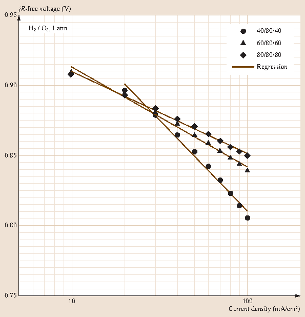
Tafel slope analysis by linear regression of jR-free voltage versus $\log(j)$ data acquired for three reactant humidity levels: low (40 ∕ 80 ∕ 40, 16 % RH), medium (60 ∕ 80 ∕ 60, 42 % RH), and high (80 ∕ 80 ∕ 80, 100 % RH)
Full size image

Figures 20.18 and 20.19 summarize the performance data on linear and semi-log plots, respectively. Different features of the performance of the fuel cell are highlighted by plotting the data in these two formats. The former voltage–current density plot shows the linear relationship observed at moderate current densities whereas the semi-log format highlights the activation-controlled and mass-transport controlled regions at low and high current densities, respectively. Both figures demonstrate the effect of temperature and oxidant concentration on the performance of the cell. For this reason, both types of plots are commonly used when evaluating the V–j behavior of fuel cells.

The effect of operating temperature (${\mathrm{25}}\,{\mathrm{{}^{\circ}C}}$ versus ${\mathrm{80}}\,{\mathrm{{}^{\circ}C}}$, at 100 % RH) on cell performance and membrane resistance for a H₂ PEM cell operating on pure O₂ or air is shown in Fig. 20.18. Measured OCV and theoretical reversible potential at ${\mathrm{80}}\,{\mathrm{{}^{\circ}C}}$ are slightly lower than the corresponding values at ${\mathrm{25}}\,{\mathrm{{}^{\circ}C}}$. (There is also the expected oxidant composition effect on OCV and E_theor.) The temperature effect on these properties is primarily due to the higher concentration of reactants (H₂ and O₂) when fed at lower temperatures under saturated moisture conditions (100 % RH). The absolute water content of a gas increases with temperature; thus, increasing the temperature of the feed gas decreases the relative proportion of reactant in the water-vapor saturated gas. The effect of reduced reactant concentration on E_theor can be predicted by examination of the Nernst equation

$$E_{\text{theor}}\propto\log\left(\frac{p_{\mathrm{H_{2}}}p_{\mathrm{O_{2}}}^{1/2}}{p_{\mathrm{H_{2}O}}}\right)\;.$$

(20.5)

Figure 20.18 shows that under fully hydrated conditions, membrane resistance decreases with increasing temperature. The temperature dependence of the ohmic resistance of the membrane is related to the mobility of the protons, which increases with increasing temperature.

Although the OCV and E_theor decrease with increasing temperature, elevated temperatures favor faster reaction kinetics on the catalyst surface, increased diffusion through the GDL, and lower membrane resistance. The net result is improved overall cell performance at ${\mathrm{80}}\,{\mathrm{{}^{\circ}C}}$ in comparison to ${\mathrm{25}}\,{\mathrm{{}^{\circ}C}}$ under fully saturated conditions as demonstrated by the power density curves shown in Fig. 20.24.

The effect of reactant humidity on the performance of the cell is shown in Fig. 20.20. In each case, the cell was operated at ${\mathrm{80}}\,{\mathrm{{}^{\circ}C}}$ while the anode and cathode gas humidifier tanks were both set at either 40, 60 or ${\mathrm{80}}\,{\mathrm{{}^{\circ}C}}$, corresponding, respectively, to low (16 % RH), moderate (42 % RH) and high (100 % RH) humidity conditions within the cell. The performance of the cell is a strong function of the humidity of the reactants (Table 20.4).

Table 20.4 Operating conditions, and theoretical and experimental results for PEM fuel cell

Full size table

The performance of the cell at low humidity conditions is independent of the oxidant concentration. That is, the V–j data are nearly identical using oxygen and air at low humidity (i. e., 40 ∕ 80 ∕ 40). A significant improvement in performance when operating with pure oxygen in comparison to air is observed only when the cell was well-humidified indicating that the resistance of the membrane dominates the performance of the cell under dehydrated or low RH conditions.

Figure 20.20 indicates that the membrane resistance, determined using the current interrupt technique, increases by greater than an order of magnitude between the high and low humidity conditions (i. e., 0.1 versus ${\mathrm{1.2}}\,{\mathrm{{\Upomega}{\,}cm^{2}}}$ at 100 % RH and 16 % RH, respectively). For a given humidity condition, the membrane resistance is independent of the oxidant composition; hence, only resistance data for oxygen is shown.

Figure 20.21 further demonstrates the influence of reactant moisture content on the performance of the PEM fuel cell by showing the effect of just anode as well as anode and cathode reactant humidification. It is evident, for example, that humidification of the fuel alone dramatically improves the performance of the cell by decreasing the resistance of the membrane (e. g., compare the conditions 60 ∕ 80 ∕ 60 and 80 ∕ 80 ∕ 60). Arguably, humidification of the hydrogen fuel had a greater impact on the performance of the cell than did humidification of the oxygen. This can be rationalized by considering that water is produced at the cathode whereas it is removed at the anode by osmotic drag through the membrane. In practice, control of the water content of both anode and cathode feed streams is performed to optimize the performance of the cell.

2.2.2 Analysis of Electrode Kinetics

The effect of cell humidification on reaction kinetics is demonstrated by Tafel analysis, which was presented in detail in Sect. 20.2.1. The Tafel slope is given by the slope of the cell voltage (corrected for membrane resistance) plotted as a function of the logarithm of the current density. The Tafel slope is obtained by linear regression of the data.

Figure 20.22 shows the Tafel plots for a fully humidified H₂/O₂ cell operating at four temperatures. Experimental Tafel slopes were 59.0, 60.2, 61.8, and 58.6 mV/dec at 25, 40, 60, and ${\mathrm{80}}\,{\mathrm{{}^{\circ}C}}$, respectively. The low temperature results correspond quite well with theoretical predictions of the Tafel slope although they tend to diverge at the higher temperatures ($b_{\text{c,theor}}=59.2$, 62.0, 66.1, 70.1 mV/dec, respectively).

The effect of humidity on the electrode kinetics is shown in Fig. 20.23 wherein Tafel analysis is performed on data acquired at low (40 ∕ 80 ∕ 40, 16 % RH), medium (60 ∕ 80 ∕ 60, 42 % RH), and high (80 ∕ 80 ∕ 80, 100 % RH) humidity levels. The apparent resistance to the ORR increased significantly at low humidity levels, as indicated by the large Tafel slope ($={\mathrm{129}}\,{\mathrm{mV/dec}}$). With increasing reactant humidity the electrode kinetics became more facile (i. e., 71.2 and 58.6 mV/dec at moderate and high humidity, respectively). This apparent increase in the Tafel slope is perhaps due to enhanced ohmic and mass transport losses within the cathode catalyst layer as the RH is lowered. Data at lower current density would be desirable to define the true cathode kinetics. A change in the mechanism of oxygen reduction cannot be ruled out.

The results attained in these experiments indicate that unless the effects of humidity on the electrode kinetics are specifically being investigated, electrode kinetics should be studied using well humidified conditions and pure oxygen as the oxidant.

2.2.3 Summary

The experiments described in this part are intended to instill understanding and experience in employing electrochemical test methods to determine the performance characteristics of a hydrogen-fueled PEMFC. The performance of the fuel cell has been presented via voltage versus current density and resistance versus current density plots.

A detailed data analysis and discussion is presented to acquaint the reader with concepts related to fuel cell reactant consumption rates and utilization. Some of the experiments proposed allow the reader to evaluate the performance of PEM fuel cell as a function of temperature, reactant gas humidity levels, oxygen concentration and stoichiometry with an emphasis on the effects of varying these parameters on electrode kinetics, mass transport limitations, and cell resistance.

The measured OCV is shown to be less than the theoretical maximum potential (E_theor) in all cases, and both values decrease with declining oxygen concentration. The OCV is less than E_theor because in practice, parasitic oxidation reactions at the cathode lead to a mixed potential that is lower than the electrode potential predicted based solely on the ORR. Oxidation of fuel that crosses over through the membrane and oxidation of the cathode materials (e. g., carbon support) both contribute to this mixed potential.

Activation polarization due to kinetic limitations dominate at low current densities (0–$\mathrm{100\,mA/cm^{2}}$). Analysis of the polarization data in this activation region allows to estimate the Tafel slope and the exchange current density. Ohmic losses dominate at intermediate current densities (100–$\mathrm{1000\,mA/cm^{2}}$) and are a resultant of ionic and electronic resistances. The membrane resistance is typically relatively constant up to about ${\mathrm{1000}}\,{\mathrm{mA/cm^{2}}}$ and is independent of oxidant composition. At larger current densities, the ohmic resistance of the membrane increases slightly due to dry-out of the membrane on the anode side. Dry-out of the membrane within the PEM fuel cells is a common phenomenon at high current densities and occurs because water molecules associated with migrating protons are dragged from the anode to the cathode at a higher rate than they can diffuse back from the cathode (where water is also produced). This phenomenon is more clearly seen with thicker membranes, such as Nafion 117, than with thin membranes such as Nafion 211 used here.

Mass transport limitations due to insufficient supply of oxygen to the surface of the cathode are observed at higher current densities (more than ${\mathrm{1000}}\,{\mathrm{mA/cm^{2}}}$) and dominate the polarization in this region. The limiting current density is the maximum attainable current density in this regime and depends on the oxygen concentration in the oxidant stream, the flow rates, the properties of the diffusion media, and the cell design.

3 Application of a Fuel Cell Empirical Model

Fuel cell research and development is currently focused on material cost reduction in conjunction with optimization of fuel cell design for improved performance and durability. To achieve the required performance and cost goals, there is a strong need to identify, understand, control, predict, and optimize the various thermodynamic, kinetic and transport processes that occur on disparate length scales during fuel cell operation. Optimization of fuel cell technology will not be achieved by experimental analysis alone because of the large number of interdependent and complex processes and structure–property–performance relationships involved. Modeling of fuel cells is used to reduce development time and cost while increasing the scientific understanding of this complex technology by facilitating identification of the critical parameters that have the largest impact on performance. Wang recently reviewed the status of fuel cell modeling efforts [20.7].

Although comprehensive modeling of a fuel cell system is beyond the scope of this book, a simple model describing voltage–current characteristics of the fuel cell can be introduced and implemented to test for 1.) its ability to fit the data, and 2.) its utility as an analytical tool.

A common method to determine cell voltage losses is least squares fitting of an analytical expression incorporating the three main sources of loss to the experimental performance data. The simplified empirical model employed here is based on the work of Srinivasan and coworkers [20.10, 20.11, 20.12, 20.8, 20.9].

The complete relationship between the cell voltage and current-dependent polarization losses can be described by

$$\begin{aligned}\displaystyle V_{\text{cell}}&\displaystyle=E_{\text{theor}}-(\eta_{\text{act,c}}+\eta_{\text{act,a}})-\eta_{\Upomega}\\ \displaystyle&\displaystyle\quad\;-(\eta_{\text{conc,c}}+\eta_{\text{conc,a}})\;,\end{aligned}$$

(20.6)

where the three primary sources of polarization, previously presented are listed here.

1.
Activation polarization (η_act). The Tafel equation (20.4) describes the relationship between the current density j and activation polarization η_act at large overpotentials.
2.
Ohmic polarization (${\eta}_{\Upomega}$). Voltage losses due to ionic and electronic transport resistance and contact resistance as described by a simplified form of Ohm’s law,
$$\eta_{\Upomega}=jR_{\Upomega}\;,$$
(20.7)
where $R_{\Upomega}$ is the resistance in ${\mathrm{\Upomega{\,}cm^{2}}}$.
3.
Concentration polarization (η_conc). Mass transport polarization losses can be described by
$$\eta_{\text{conc}}=C\log\left(\frac{j_{\text{lim}}-j}{j_{\text{lim}}}\right)\;.$$
(20.8)
Here, j_lim in $\mathrm{A/cm^{2}}$ is the maximum achievable current density based on the Fickian diffusion of reactant to the electrode surface at which the concentration of reactant is assumed to be zero [20.13]. The parameter C is related to the Tafel slope by
$$C=2.303\frac{RT}{nF}\;,$$
(20.9)
where R, T, n, and F have their usual meaning. Equation (20.8) indicates that η_conc becomes a very large negative number as j approaches j_lim and describes the source of the rapid decrease in cell potential in the regime where the reaction consumption rate (given by the current density) is dictated by transport of reactant to the active surface sites.

3.1 Model Application and Analysis

To perform the simplified modeling analysis, we make the following assumptions:

Polarization at the anode (activation, ohmic, and concentration) is negligible in comparison to cathodic contributions. This assumption is generally justified for pure H₂ operation, but will not hold for reformate or direct methanol operation.
At the cathode, activation-controlled kinetics can be described by Tafel behavior (20.4).
Mass transport losses (concentration polarization) can be described by (20.8).
Ohmic resistance is independent of current density. (Resistance is known to increase at high current densities due to dehydration so the validity of this assumption should be regarded with some skepticism, at least under some conditions.)
All of the polarization losses can be separated and do not interact.
Ohmic losses in the cathode are negligible.

Equation (20.10) is the result of applying the earlier assumptions and substituting the respective polarization relationships into (20.6),

$$\begin{aligned}\displaystyle V_{\text{cell}}&\displaystyle=E_{\text{theor}}-b_{\text{c}}\log\left(\frac{j}{j_{\text{o,c}}}\right)\\ \displaystyle&\displaystyle\quad\;-jR_{\Upomega}+C_{\text{c}}\log\left(\frac{j_{\text{lim,c}}-j}{j_{\text{lim,c}}}\right)\;.\end{aligned}$$

(20.10)

Here, the subscript c is used to reinforce the assumption that polarization losses are attributed to cathodic processes, either activation or mass transport (in addition to ohmic effects). The exchange current density is a constant for a given reaction–electrode system, and as such (20.10) can be rearranged to give

$$\begin{aligned}\displaystyle V&\displaystyle=E_{\text{theor}}+A_{\text{c}}-b_{\text{c}}\log(j)-jR_{\Upomega}\\ \displaystyle&\displaystyle\quad\;+C_{\text{c}}\log\left(\frac{j_{\text{lim,c}}-j}{j_{\text{lim,c}}}\right)\;,\end{aligned}$$

(20.11)

where $A_{\text{c}}=b_{\text{c}}\log j_{\text{o,c}}$. The five fitted parameters are: ($E_{\text{theor}}+A_{\text{c}}$), b_c, $R_{\Upomega}$, C_c, and j_lim,c. From this empirical model, we can estimate physiochemically meaningful parameters including the cathodic Tafel slope and limiting current density, and the cell ohmic resistance.

Table 20.5 summarizes theoretical, experimental, and empirical modeling results for a PEM fuel cell operating at ${\mathrm{80}}\,{\mathrm{{}^{\circ}C}}$, ${\mathrm{25}}\,{\mathrm{{}^{\circ}C}}$, and with a range of oxidant concentrations. Theoretical parameters include the reversible potential and Tafel slope (assuming ${\upalpha}_{\text{c}}=0.5$). Experimental values include the OCV, cathodic Tafel slope from the analysis of low-current density data regression (e. g., performed in Sects. 20.2.1 and 20.2.2), and the ohmic resistance ($R_{\Upomega}$) from current interrupt.

Table 20.5 Theoretical, experimental, and empirical model fit values for kinetic, ohmic, and transport parameters for a H₂ PEMFC operating at 80 and ${\mathrm{25}}\,{\mathrm{{}^{\circ}C}}$ with a range of oxygen concentrations

Full size table

Values for the adjustable parameters (($E_{\text{theor}}+A_{\text{c}}$), b_c, $R_{\Upomega}$, C_c, and j_lim,c) obtained via regression of polarization data (V versus j) using an equation of the form given by (20.11) are also summarized in Table 20.5. The empirical model was fitted to the experimental data using nonlinear regression software; fitting curves generated using this model had correlation coefficients in excess of 0.992. The model, therefore, is excellent as a fitting function for fuel cell performance curves from which values can be interpolated or extrapolated. For example, one can estimate the limiting current density in cases where data is insufficient to estimate it experimentally. For comparison, the fitted and experimental data are presented in Fig. 20.25a,b. The accuracy of the estimation, however, is in question as is discussed later.

The regression-generated values for $R_{\Upomega}$ can be compared to experimentally measured values. Ohmic resistance calculated using (20.7) was consistent (${\pm}{\mathrm{15}}\%$) with experimental values measured by current interrupt at ${\mathrm{25}}\,{\mathrm{{}^{\circ}C}}$; greater discrepancy (−30 to $+{\mathrm{50}}\%$) between predicted and measured values was observed for the ${\mathrm{80}}\,{\mathrm{{}^{\circ}C}}$ data set. The discrepancies suggest that $R_{\Upomega}$ in (20.7) is not strictly representative of the membrane resistance but in fact includes additional losses other than the ohmic resistance of the membrane. As noted earlier, although $R_{\Upomega}$ in the model is assumed to be independent of current density, it is well established that in actual fuel cell operation, membrane resistance is a function of operating conditions such as current density and gas composition. $R_{\Upomega}$ is therefore partially determined by mass transport effects [20.11, 20.12]. Because the ohmic resistance of the cell is not a fixed value, the resistance $R_{\Upomega}$ determined from a fit using the empirical model should more appropriately be considered pseudo-ohmic [20.14].

Values for the Tafel slope predicted from theory can also be compared to values obtained via regression using (20.11) (the full empirical model) and (20.4) (the Tafel equation) to test the model’s analytical capability. The theoretical cathodic Tafel slope b_c can be calculated using (20.3).

In this equation, ${\upalpha}_{\text{c}}$ is the transfer coefficient and is assumed equal to 0.5 for the ORR [20.5]. According to this theory, the Tafel slope should be 59 mV/dec and 70 mV/dec at 25 and ${\mathrm{80}}\,{\mathrm{{}^{\circ}C}}$, respectively. Tafel slope analysis using experimental data (i. e., jR-free V_cell versus $\log j$) based on the Tafel equation was performed as part of Sects. 20.2.1 and 20.2.2.

Table 20.5 shows that b_c values derived from the regression based on the empirical model were ${\pm}{\mathrm{30}}\%$ of the theoretical value. In contrast, those obtained from the Tafel equation via linear regression of jR-compensated $V_{\text{cell}}-\log j$ data in the low current density region tended to more closely match theoretical predictions. These results indicate that Tafel slopes are more accurately obtained from raw data using the Tafel equation in comparison to the results extracted from a multiparameter empirical model. One might suggest some physical reasons for the discrepancy, such as the existence of diffusion or resistive losses in the cathode catalyst layer of the electrode. We may argue, however, that the model is too flexible to assign any physical significance to the values of the parameters obtained by force fitting to experimental data (i. e., a large range of values for each parameter in the empirical model yield a reasonably good fit). The model exhibits limited reliability in predicting true physical behavior of individual contributions to the polarization curve, and therefore must be used with utmost caution.

Williams et al presented a more thorough and meaningful methodology to analyze the sources of polarization within PEM fuel cells [20.4].

3.2 Summary

In this section, we have examined the application of a simple empirical model to describe the voltage–current density characteristics of the fuel cell, and evaluated the model in terms of its ability to fit the data and its utility as an analytical tool. The model incorporates three main sources of voltage loss: activation polarization (η_act), ohmic polarization (${\eta}_{\Upomega}$), and concentration polarization. We employ the following assumptions in the application of the model:

1.
Polarization at the anode (activation, ohmic and concentration) is negligible in comparison to cathodic contributions.
2.
The Tafel equation can be used to describe cathode kinetics.
3.
Ohmic resistance is independent of current density.
4.
Ohmic losses in the electrodes are negligible.
5.
All of the polarization losses are separable and do not interact.

The model fits the experimental data reasonably well. However, given that it is a multiparameter fit, care must be taken to identify whether each parameter is indeed sensitive and can be effectively used to identify main sources of polarization.

4 Fuel Crossover and Electrochemical Surface Area

This section examines the evaluation of two key properties of H₂ PEM fuel cells: (a) Hydrogen fuel crossover through the membrane and (b) electrochemically active area of the electrode. These techniques are based on linear potential sweep methods treated in detail by standard texts on electrochemical techniques [20.13, 20.15].

4.1 Hydrogen Crossover and Internal Short Circuit

Crossover of fuel (hydrogen) from one electrode to the other by permeation through the electrolyte degrades the performance of the cell by reducing the OCV of cell through induced mixed potentials and by decreasing fuel efficiency. This phenomenon is referred to as fuel crossover. Oxidant crossover can also occur through a similar mechanism (albeit in the opposite direction).

Direct conduction of electrons between the electrodes through the electrolyte is also a source of loss within a fuel cell. Although the electrolyte of the cell is designed to be electrically insulating and ionically conducting, a finite amount of electron conduction can also occur, especially if small portions of the individual electrode contact one another due to electrolyte thinning. As with crossover, excessive electronic conduction through the electrolyte results in degradation of cell performance.

Fuel crossover and internal short circuits are essentially equivalent. The crossover of one hydrogen molecule resulting in the loss of two electrons is the same as the loss occurring from the conduction of two electrons from the anode to the cathode. A fuel crossover current of ${\mathrm{1}}{-}{\mathrm{2}}\,{\mathrm{mA/cm^{2}}}$ may be acceptable if the operating current density of the system is around ${\mathrm{400}}\,{\mathrm{mA/cm^{2}}}$. This proportion equates to a loss of efficiency of 0.25-0.5 %.

To experimentally determine the fuel crossover, a suitable inert gas such as nitrogen is used to purge the fuel cell cathode while hydrogen is passed through the fuel cell anode. The potential of the fuel cell cathode (now the working electrode (GlossaryTerm

WE

)) is swept by means of a linear potential scan to potentials at which any hydrogen present is instantaneously oxidized. Such experiments are typically referred to as linear sweep voltammetry (LSV) experiments. The output of working electrode (WE) current versus WE potential can be used to derive the hydrogen crossover flux from Faraday’s law. The diffusion-limiting current that is attained at electrode potentials is directly related to the hydrogen crossover flux through Faraday’s law. The results of such an experiment are shown in Fig. 20.26.

The presence of significant internal shorting within a fuel cell can also be detected from the results of this experiment, and is manifested as a positive slope in the current potential plot (an example of this is shown in Fig. 20.26).

A simpler but less informative approach to detection of crossover is performed by shutting off the cathode oxygen supply and monitoring the OCV of the fuel cell for approximately 2 min [20.16]. Leaking hydrogen gas through membrane to the cathode will react with the available oxygen thereby decreasing the concentration of oxidant. Nernst’s law states that the OCV is a function of reactant concentration. Therefore, a decrease in cell voltage arising from the decrease in oxygen concentration indicates fuel crossover. Although relatively easy to perform and requiring no special equipment (such as a potentiostat needed for the method described above and performed below), this approach has the disadvantages that the rate of crossover is unknown and the presence or absence of an electrical short is also not indicated.

4.1.1 Electrochemical Surface Area (ECSA) of Electrode Catalyst

Cyclic voltammetry (GlossaryTerm

CV

) is a common diagnostic tool for characterizing the electrode properties. A typical PEMFC electrocatalyst layer consists of a mixture of carbon-supported Pt and a proton conducting material such as Nafion (or alternate ionomers). The carbon support enhances the electronic conductivity and provides better Pt dispersions, while the ionomer serves to bind the electrode layer and facilitate proton conduction through the layer. The electrochemical activity of the electrode is dependent on the extent of formation of a three phase boundary where reactants, conducting material and active catalyst sites are in contact with one another.

The technique for determining the electrochemical surface area (GlossaryTerm

ECSA

) of a catalyst in an electrode by CV analysis has been used for several decades. The procedure involves cycling the electrode of interest over a voltage range such that charge-transfer reactions are adsorption limited. That is, the electrode potential is such that the number of reactive surface sites can be obtained by recording the total charge required for monolayer adsorption/desorption. Common reactions used when characterizing PEM fuel cell electrodes are the hydrogen adsorption/desorption (GlossaryTerm

HAD

) reaction,

$$\mathrm{Pt}+\mathrm{H^{+}}+\mathrm{e^{-}}\leftrightarrow\mathrm{Pt}-\mathrm{H}_{\text{ads}}$$

(20.12)

or the oxidative stripping of adsorbed carbon monoxide (GlossaryTerm

CO

) [20.17],

$$\mathrm{Pt}-\mathrm{CO}_{\text{ads}}+\mathrm{H_{2}O}\rightarrow\mathrm{Pt}+\mathrm{CO_{2}}+2\mathrm{H^{-}}+2\mathrm{e^{-}}\;.$$

(20.13)

Fuel cell electrodes may be examined for their electrocatalytic performance by ex situ or in situ voltammetry experiments. In the case of ex situ experiments (also known as half-cell experiments), the properties of the electrode are evaluated using a standard three-electrode cell with an aqueous solution of acid (typically 0.1 M HClO₄) used to simulate the proton-conducting electrolyte in a PEMFC. Half-cell experiments are a convenient and relatively fast method of screening electrocatalysts.

In situ experiments use a two-electrode configuration in which one of the electrodes of the fuel cell serves as both a pseudo-reference electrode and a counter electrode (GlossaryTerm

CE

). Typically, the electrochemical activity of the fuel cell cathode is of most interest because of the sluggish kinetics of the ORR. Therefore, this electrode is often chosen to be the WE. The fuel cell anode is used as the CE/RE with the inherent assumption that polarization of this electrode is small relative to the polarization imposed on the fuel cell cathode. The currents obtained in the ECSA tests are small and justify this assumption.

While performing the in situ CV experiment, the fuel cell cathode (WE) is purged with nitrogen, while hydrogen is fed to the anode compartment (counter/reference electrode). Akin to the LSV experiment, the voltage of the WE is swept to high potentials and any hydrogen molecules that cross over through the membrane are instantly oxidized. In contrast to the LSV experiment, in a CV experiment, an additional reverse potential scan is performed. During the reverse potential sweep, proton (H${}^{+}$) reduction to adsorbed H (H_ads) occurs in the potential region 0.4–0.05 V versus the CE/RE (i. e., toward the end of the reverse sweep). An example of such a voltammogram for a Pt electrode is shown in Fig. 20.27.

The reaction of interest [20.18] is the electrochemical reduction of protons (H${}^{+}$) and subsequent deposition of atomic hydrogen on the surface of the platinum catalyst. The atomic hydrogen adsorption charge density (q in $\mathrm{C/cm^{2}}$) due to this reaction can be determined from the CV scan. The ECSA of the Pt catalyst [20.17] is calculated from the charge density, the generally accepted quantity for the charge to reduce a monolayer of protons on Pt (${\Upgamma}={\mathrm{210}}\,{\mathrm{{\upmu}C/cm^{2}}}$ Pt [20.19, 20.20]), and the Pt content (i. e., loading) in the electrode (L in $\mathrm{g{\,}Pt/cm^{2}}$ electrode),

$$\mathrm{ECSA}\;{\mathrm{cm^{2}Pt/gPt}}=\frac{q}{\Gamma L}\;.$$

(20.14)

The ratio of ECSA to the specific area of the Pt used to make the MEA (also in $\mathrm{cm^{2}Pt/gPt}$) is the fraction of catalyst that is electrochemically available to participate in the electrode reactions. This ratio is referred to as utilization. Obviously, higher catalyst utilization is better.

Integration of the hydrogen desorption/adsorption peaks that result as a consequence of the forward and reverse scans, respectively, may be used to estimate the electrochemically active surface area of the electrocatalyst. The shaded area represents the total charge arising from hydrogen adsorption. The baseline (current density) is the capacitive current due to charging of the electrode double layer.

During the CV experiment, the potential of the WE is swept first in the anodic direction to oxidize the adsorbed hydrogen (H_ads) to H${}^{+}$ and then in the cathodic direction to electrochemically reduce the H${}^{+}$ back to H_ads. Alternating anodic and cathodic currents occur at the electrode. Experimental results are usually plotted as a graph of current or current density versus the WE potential, and a voltammogram like is obtained. The voltammogram exhibits multiple peaks associated with both the oxidation and reduction reactions. The sweep rate is increased in a CV experiment in comparison to the LSV performed for the crossover experiment to augment the peak size.

Both RH of the gases to which the electrode is exposed, and the electrode temperature impact the measured ECSA. Fully or supersaturated (${\geq}{\mathrm{100}}\%$ RH) are generally used. The ECSA experiment should be conducted on membrane electrode assemblies that have been through a break-in procedure to fully active the electrode.

The flow rate of nitrogen (or other inert gas) on the WE during the voltage sweep can significantly influence the shape of the adsorption/desorption curve and therefore the ECSA measurement [20.21]. The artifact was attributed to the rate of mass transfer of molecular hydrogen (H₂) away from the WE during the voltage scan. With increasing N₂ purge rate, molecular hydrogen is more readily swept from the WE surface, decreasing the partial pressure (concentration) of H₂ at the WE thereby increasing the reversible Nernst potential for hydrogen evolution. Operating conditions that decrease the H₂ concentration at the WE increase the reversible potential for hydrogen evolution, which confounds accurate measurement of the H-adsorption/desorption process. Therefore, relatively low nitrogen flow rate, $\approx{\mathrm{1}}\,{\mathrm{sccm/cm^{2}}}$ of active area is preferred.

Utilization is the fraction of the catalyst’s surface area that is electrochemically available in the MEA, obtained by CV on an MEA, to the specific surface area of the catalyst determined by ex situ methods such as particle size analysis. Note that this value represents an idealized condition because the current density is very low and transport resistances that arise at higher current are negligible. In a fuel cell operating at high current density, transport resistances for oxygen and/or protons (H${}^{+}$) decrease the amount of platinum that participates in the cathode reaction [20.22].

The procedure described here is the most simple for measuring the ECSA in an operating fuel cell. However, it does suffer from some artifacts, such as arising from concentration cell effects and hydrogen crossover. These can be mitigated using modified procedures. Details of those methods can be found in the nice work of Edmundson and Busby on this topic [20.23].

4.1.2 Procedure

Assemble the MEA, setup the fuel test cell station and connect all gas lines.

The fuel cell anode is purged with 0.20 SLM H₂ at 100 % RH, and the fuel cell cathode with 0.5 SLM N₂ at 100 % RH.

The potentiostat leads are connected as shown in Fig. 20.28 and any current or sense leads from the test station are disconnected.

To measure hydrogen crossover flux a linear sweep voltammetry LSV or linear polarization experiment from 0 V (vs. open circuit) to 0.8 V (vs. reference) at 2 mV/s is performed.

To determine the ECSA of the electrode catalyst, a CV experiment from 0.05 V (vs. reference) to 1.0 V (vs. reference) at 20 mV/s is performed.

4.2 Hydrogen Crossover Test via LSV

Figure 20.26 shows a typical result for an LSV experiment performed under the cell conditions described wherein the current density is shown as a function of voltage. This plot can be used to compare the response of a high-quality pristine cell to that of degraded cell. The pristine cell exhibited a limiting current density (j_lim) of 1.1 and ${\mathrm{1.4}}\,{\mathrm{mA/cm^{2}}}$ at 35 and ${\mathrm{75}}\,{\mathrm{{}^{\circ}C}}$, respectively, which is consistent with an increase in the permeability of hydrogen through the membrane with temperature.

The limiting current density is proportional to the rate of H₂ crossover from the anode to the cathode through the membrane. Applying Faraday’s law to determine the limiting hydrogen crossover flux ($\dot{N}_{\mathrm{H_{2}}}$) at ${\mathrm{35}}\,{\mathrm{{}^{\circ}C}}$,

$$\begin{aligned}\displaystyle\dot{N}_{\mathrm{H_{2}}}&\displaystyle=\frac{j_{\text{lim}}}{nF}=\frac{({\mathrm{1.1\times 10^{-3}}}\,{\mathrm{A/cm^{2}}})}{({\mathrm{2}}\,{\mathrm{eq./mol}})({\mathrm{96485}}\,{\mathrm{C/eq.}})}\frac{\mathrm{C}}{{\mathrm{As}}}\\ \displaystyle&\displaystyle={\mathrm{5.7\times 10^{-9}}}\,{\mathrm{mol/(s{\,}cm^{2})}}\;.\end{aligned}$$

(20.15)

The pristine cell also did not exhibit an internal short as evidenced by the absence of an increasing current with increasing polarization beyond 0.15 V versus RE/CE.

In contrast to the pristine cell, the degraded cell exhibited significant hydrogen flux through the membrane ($j_{\text{lim}}={\mathrm{5.5}}\,{\mathrm{mA/cm^{2}}}$, $\dot{N}_{\mathrm{H_{2}}}={\mathrm{2.85\times 10^{-8}}}\,{\mathrm{mol/(s{\,}cm^{2})}}$). Figure 20.26 also shows that the degraded cell demonstrated an internal electronic short circuit between the two electrodes. The presence of an internal short within the cell is indicated by the linear, positive slope on the current density versus potential curve. The resistance of the electrical short is estimated to be ${\mathrm{333}}\,{\mathrm{\Upomega{\,}cm^{2}}}$ and is obtained from the inverse of the slope of the line in the region 0.2–0.4 V versus CE/RE.

4.3 Electrochemically Active Surface Area and Catalyst Utilization Evaluation

Figure 20.27 shows a typical cyclic voltammogram. The reaction of interest is given by (20.12) and the electrochemically active surface area of the platinum catalyst in the cathode which can be estimated from this figure using (20.14).

The cyclic voltammogram of a ${\mathrm{50}}\,{\mathrm{cm^{2}}}$ cell is shown in Fig. 20.27, where the data is plotted as current density versus potential. The scan rate (ν) for this experiment was 0.04 V/s. The reduction reaction within the potential range 0.06 to 0.40 V [20.19] which corresponds to a time of 8.5 s (i. e., ${\mathrm{0.34}}\,{\mathrm{V}}/{\mathrm{0.04}}\,{\mathrm{V/s}}={\mathrm{8.5}}\,{\mathrm{s}}$).

Recall that the electrode double layer behaves in part like a capacitor. Because the electrode potential is changing with time, non-Faradaic current exists due to charging of the electrode interface, and this current is directly proportional to the scan rate,

$$j_{\text{dl}}=C\frac{\mathrm{d}E}{\mathrm{d}t}=C_{\text{dl}}\nu\;,$$

(20.16)

where C_dl is the capacitance of the double layer per unit area in $\mathrm{C/cm^{2}}$.

The charge associated with double-layer charging must be accounted for in the analysis to avoid overestimating the charge attributed to the electrocatalytic activity. From Fig. 20.29, we note that the baseline double-layer charging and discharging current densities ($j_{\text{dl charging}}$) were ${\mathrm{2.3}}\,{\mathrm{mA/cm^{2}}}$ in the potential range of 0.4 to 0.06 V where no Faradaic processes are occurring. The double-layer charging charge density over the electrode potential region of interest was ${\mathrm{19.6}}\,{\mathrm{mC/cm^{2}}}$ ($={\mathrm{2.3}}\,{\mathrm{mA/cm^{2}}}\times{\mathrm{8.5}}\,{\mathrm{s}}$). The double-layer charging current density is displaced in the positive direction by an amount equal to the fuel crossover current density ($j_{\text{x-over}}$). Also note that the mean potential at which the oxidation and reduction reaction occurs during, respectively, the forward and reverse scans, is displaced because of the hydrogen crossover.

The net charge density associated with the reduction of protons to adsorbed hydrogen is estimated at ${\mathrm{43.9}}\,{\mathrm{mC/cm^{2}}}$, shown as the hatched region in Fig. 20.29. Applying (20.14), the electrochemically active surface area of Pt is

$$\begin{aligned}\displaystyle\mathrm{ECSA}&\displaystyle=\left({\mathrm{43.9}}\,{\mathrm{mC/cm^{2}}}\,\mathrm{MEA}\right)\\ \displaystyle&\displaystyle\quad\;\times\left[({\mathrm{210\times 10^{-3}}}\,{\mathrm{mC/cm{\,}Pt}})\right.\\ \displaystyle&\displaystyle\quad\;\times\left.({\mathrm{0.4\times 10^{-3}}}\,{\mathrm{g{\,}Pt/cm^{3}}}\mathrm{MEA})\right]^{-1}\\ \displaystyle&\displaystyle={\mathrm{5.23\times 10^{5}}}\,{\mathrm{cm^{2}{\,}Pt/g{\,}Pt}}={\mathrm{52.3}}\,{\mathrm{m^{2}{\,}Pt/g{\,}Pt}}\;.\end{aligned}$$

(20.17)

Assuming that the specific surface area of the Pt used in the manufacturing of the MEA was ${\mathrm{70}}\,{\mathrm{m^{2}{\,}Pt/g{\,}Pt}}$, this analysis indicates that 75 % of the Pt is electrochemically active in the cathode. Thus, catalyst utilization is 75 % for this MEA.

4.3.1 Summary

In this part, we examine, through laboratory examples, the evaluation of two key properties of H₂ PEM fuel cells: hydrogen fuel crossover through the membrane and electrochemically active area of the electrode. The techniques used are LSV and CV, and are of high importance for the characterization and proper evaluation of PEM fuel cells.

The method for determining the ECSA of a catalyst in an electrode by CV involves cycling the electrode of interest (mostly the cathode of the PEMFC) typically from 0.05 to 0.8 V versus RE/CE at a scan rate usually in the interval 20–50 mV/s. The atomic hydrogen adsorption charge density can be determined from the CV scan. The ECSA of the Pt catalyst is calculated from the charge density, the generally accepted quantity for the charge to reduce a monolayer of protons on Pt (${\mathrm{210}}\,{\mathrm{{\upmu}C/cm^{2}{\,}Pt}}$), and the Pt content in the electrode. The charge associated with double-layer charging and hydrogen crossover currents must be accounted for in the analysis, by proper selection of the integration baseline (as shown in Fig. 20.29), to avoid overestimating the charge attributed to the electrocatalytic activity.

Platinum utilization is the ratio of the catalyst surface area that is electrochemically available in the MEA, as obtained by CV on an MEA, to the specific surface area of the catalyst determined by ex situ methods such as particle size analysis or chemisorption measurements.

Fuel crossover through the PEM degrades the performance of the cell by reducing the OCV through induced mixed potentials and by decreasing fuel efficiency. Over time, this also contributes to electrolyte degradation. Direct conduction of electrons between the electrodes through the electrolyte (short circuit) is also a source of loss within a fuel cell. Fuel crossover and internal short circuits are essentially equivalent and can be estimated using LSV (scanning from OCV to 0.4 V versus RE/CE). The diffusion limiting current that is attained at electrode potentials of approximately 0.4 V is directly related to the hydrogen crossover flux through Faraday’s law. Typically, a fuel crossover current of 1 to ${\mathrm{2}}\,{\mathrm{mA/cm^{2}}}$ is acceptable. The presence of significant internal shorting within a fuel cell can also be detected from the results of this experiment, and is manifested as a positive slope in the current potential plot.

5 Impedance Spectroscopy of PEM Fuel Cells

A fuel cell is a complicated electrochemical system. The performance of a fuel cell is a complex interplay of many factors that include structural and operating characteristics of the cell. Some factors are interrelated while others are independent. Furthermore, some properties and processes occurring within the cell are responsive to changes in the cell conditions over a broad range of timescales. For example, diffusion processes occur on the order of subseconds to seconds whereas charge transfer processes (electrode reactions) can occur at much shorter time scale (submilliseconds). Because the time constants differ for different processes that take place in the fuel cell, their effects are revealed at different perturbation frequencies.

Impedance spectroscopy takes advantage of the large spectrum of timescales over which different processes within the fuel cell occur to separate their individual effects. Processes that respond slowly (or not at all) relative to other processes at one time scale can be separated from those that occur at a different timescale based on the measured impedance response of the electrochemical device over a broad range of frequencies.

In short, electrochemical impedance spectroscopy is an experimental technique that involves imposing a small sinusoidal AC voltage or current signal of known amplitude and frequency – the perturbation – to an electrochemical cell and monitoring the AC amplitude and phase response of the cell. The AC perturbation is typically applied over a wide range of frequencies, from 10 kHz or greater to less than 1 Hz; hence, the name impedance spectroscopy. The ratio and phase-relation of the AC voltage and current signal response is the complex impedance, $Z(\mathrm{i}{\omega})$. The result of an impedance spectroscopy experiment is a rich data set from which many properties of the electrochemical cell may be extracted via application of physically reasonable equivalent circuit models. Properties of the electrochemical system commonly evaluated using impedance spectroscopy include ohmic (bulk) resistance, electrode properties such as charge transfer resistance and double-layer capacitance, and transport (diffusion) effects.

Theory and concepts critical to understanding impedance spectroscopy and its practical implementation to fuel cells are covered in the following sections. Thorough treatment of this powerful, noninvasive diagnostic technique including its application to fuel cells and other electrochemical power sources are presented in [20.24]. Readers interested in more in-depth description of impedance or those intending to apply this technique for fuel cell studies are encouraged to follow-up with the referenced book as well as applicable technical articles, some of which are referenced here [20.25, 20.26, 20.27].

5.1 Impedance Theory and Practice

A sinusoidal current signal of amplitude I_AC and frequency ω can be defined as

$$I(\omega)=I_{\text{AC}}\sin(\omega t)\;,$$

(20.18)

where t is time. The output AC voltage signal from the electrochemical cell can be defined as

$$V(\omega)=V_{\text{AC}}\sin[(\omega t)-\theta]\;,$$

(20.19)

where V_AC is the amplitude of the output voltage signal and θ is the phase angle. The phase angle is the difference in the phase of the sinusoidal voltage and current signals. Figure 20.30 illustrates the voltage and current responses of a fuel cell that is subject to a sinusoidal AC input signal. In the case of an AC signal, the resistance of a circuit or electrochemical device which is not purely resistive will be a function of the frequency of oscillation of the input signal. Ohm’s law for the AC case is expressed as

$$Z(\mathrm{i}\omega)=\frac{V(\mathrm{i}\omega)}{I(\mathrm{i}\omega)}\;,$$

(20.20)

where $Z(\mathrm{i}\omega$) is the complex impedance (Ω) and i is the imaginary number

$$\mathrm{i}=\sqrt{-1}\;.$$

(20.21)

Equation (20.20) indicates that impedance is a complex value. That is, it can take on both real and imaginary components. Note that the imaginary component of the impedance is a real measurable quantity: the i is for bookkeeping purposes and allows description of the out-of-phase component of the impedance. The complex relationship of impedance is implicit so $Z(\mathrm{i}{\omega}$) is normally written as $Z({\omega}$). Although one can think of impedance as resistance to current, it is more general than that because it takes into account the phase difference between voltage and current. Equation (20.20) also indicates that impedance depends on the frequency at which it is measured; Z can change as the frequency of the AC signal changes.

Frequency in cycles per second, $f(\mathrm{Hz}={\mathrm{1/s}})$, is obtained through the relation

$$\omega=2\pi f\;.$$

(20.22)

Equation (20.20) can be written in complex notation as

$$Z=Z^{\prime}+Z^{\prime\prime}\;,$$

(20.23)

where

$$\begin{aligned}\displaystyle Z^{\prime}&\displaystyle=\mathrm{Re}(Z)=|Z|\cos\theta\\ \displaystyle&\displaystyle\quad\text{real (in-phase) component of impedance}\;,\end{aligned}$$

(20.24)

$$\begin{aligned}\displaystyle Z^{\prime\prime}&\displaystyle=\mathrm{Im}(Z)=|Z|\sin\theta\\ \displaystyle&\displaystyle\quad\text{imaginary (out-of-phase) component}\\ \displaystyle&\displaystyle\quad\text{of impedance}.\end{aligned}$$

(20.25)

The magnitude of the combined real and imaginary components can be calculated as

$$\begin{aligned}\displaystyle|Z|&\displaystyle=\sqrt{(Z^{\prime})^{2}+(Z^{\prime\prime})^{2}}\\ \displaystyle&\displaystyle\quad\text{magnitude of impedance}\;,\end{aligned}$$

(20.26)

and

$$\theta=\tan^{-1}\left(\frac{Z^{\prime\prime}}{Z^{\prime}}\right)\;.$$

(20.27)

Note that the original time-variance of V and I, the input/response signals given by (20.18) and (20.19), have disappeared in (20.23) through (20.27) and the impedance at a fixed frequency itself is time invariant as long as the system itself is time invariant.

5.1.1 Equivalent Circuits –Ideal and Distributed Elements

Although physics-based models for the impedance response of PEM fuel cells have been developed [20.25, 20.26, 20.27, 20.28, 20.29, 20.30, 20.31], they are often simplified representations of real systems (e. g., one-dimensional (1-D)), applicable at specific conditions (e. g., open circuit), and they can be complicated, requiring significant computational resources to implement. An alternative approach is to attempt to explain, understand, and extract physically meaningful properties of the electrochemical system by modeling the experimental impedance data in terms of an equivalent circuit composed of ideal resistor R, capacitor C, inductor L, and distributed circuit elements. In the equivalent circuit analog resistors represent conductive pathways for ion and electron transfer. As such, a resistor can represent the bulk resistance of a material such as the resistance of the electrolyte to ion transport or the resistance of a conductor to electron transport, or the resistance to the charge-transfer step at the surface of the electrode. Capacitors and inductors are associated with space-charge polarization regions, such as the electrochemical double layer, and adsorption and electrocrystallization processes at an electrode, respectively.

The impedance relationships of ideal electrical elements, commonly used to describe the impedance of electrochemical systems, are:

Resistor:
- Defining relationship:
  $$V=IR\;,$$
- Impedance:
  $$Z_{\text{R}}=R\;;$$
  (20.28)
Capacitor:
- Defining relationship:
  $$I=C\frac{\mathrm{d}V}{\mathrm{d}t}\;,$$
- Impedance:
  $$Z_{\text{C}}=\frac{1}{\mathrm{i}\omega C}=-\frac{\mathrm{i}}{\omega C}\;;$$
  (20.29)
Inductor:
- Defining relationship:
  $$V=L\frac{\mathrm{d}I}{\mathrm{d}t}\;,$$
- Impedance:
  $$Z_{\text{L}}=\mathrm{i}\omega L\;.$$
  (20.30)

We see that the impedance of a resistor Z_R is not a function of frequency whereas the impedance of capacitor Z_C is inversely proportional to ω and the impedance of an inductor Z_L scales linearly with frequency ω. Note the implications of these relationships in the context of an electrochemical system: the impedance of a resistor does not change with frequency; however, the impedance of a capacitor becomes very small at high frequency and very large at low frequency. Therefore, a capacitor or capacitive-like feature of an electrochemical cell behaves as a short circuit with $Z_{\text{C}}\rightarrow 0$ as ${\omega}\rightarrow{\infty}$, and at the other extreme, as an insulator with $Z_{\text{C}}\rightarrow{\infty}$ as ${\omega}\rightarrow 0$. This means that the impedance of a feature or process within an electrochemical device that behaves like a capacitor, such as the electrode double layer, becomes insignificant at high frequency. In effect, the double layer behaves as a short circuit at high frequency, where its impedance becomes negligible. Conversely, the impedance of the double layer becomes very large at very low frequency. Generally, one measures impedance over a range of frequency and it is the analysis of the resulting $Z({\omega})$ versus ω response from which one derives information about the electrical and electrochemical properties of the electrode–material system.

The Ohm’s law-like relationship between the complex voltage and current allows the impedance of a circuit with multiple elements to be calculated using the same rules as with multiple resistors. The total impedance of two elements in series is the sum of the impedances of the individual elements

$$Z_{\text{total, series}}=Z_{1}+Z_{2}\;.$$

(20.31)

Likewise, the impedance of two elements in parallel is given by

$$\frac{1}{Z_{\text{total, parallel}}}=\frac{1}{Z_{1}}+\frac{1}{Z_{2}}\;.$$

(20.32)

Note that the order of series elements in the equivalent circuit has no influence on the impedance spectrum. In the earlier given figures, the impedance response would be the same whether Z₂ follows Z₁ or Z₁ follows Z₂. While it may be helpful to arrange series circuit elements in a way that is consistent with the physical layout of the electrochemical cell, this is not strictly required. Of course, the impedance of elements arranged in parallel and in series are not the same.

The propriety of using pure resistor, capacitor, and inductor elements, which are lumped-constant quantities with ideal properties, to describe the characteristics of real electrochemical systems is tempered by the complexity of actual cells in which material properties can exhibit a distribution of values and because processes, such as diffusion, occur over a finite distance. For this reason, equivalent circuit models often invoke elements which are intended to mimic the impedance characteristics of processes or reactions which are distributed in nature. A common distributed element is the constant phase element (GlossaryTerm

CPE

), the impedance of which is defined as,

$$Z_{\text{CPE}}=\frac{1}{\Gamma(\mathrm{i}\omega)^{p}}\;,$$

(20.33)

where Γ and p are usually assumed to be frequency-independent parameters. The units for Γ are $s^{p}/{\Omega}$, while those for capacitance C are s ∕ Ω ($={\mathrm{F}}$). Hence, in the case of an ideal capacitor or resistor, p = 1 or 0, respectively, and either the magnitude of Γ equals the magnitude of C with the dimension s ∕ Ω or 1 ∕ Γ equals R in Ω (compare (20.33) to (20.29) or (20.28)). Often, a CPE is used in an equivalent circuit model in place of a capacitor to compensate for nonhomogeneity in the system. For example, a rough or porous surface can cause the double-layer capacitance to appear as a CPE with p ≈ 0.8 to 0.9. This issue is the task of extracting physically meaningful parameters conveyed by the capacitance for impedance data that is best represented in an electrical circuit model by a CPE. Examples of such parameters extracted from ideal interfacial capacitance include electrode area in the case of double-layer capacitance and surface coverage in the case of an adsorption-induced pseudo-capacitance. CPEs can also be used to model diffusional processes under some conditions [20.24].

The Warburg impedance is another common distributed impedance element. It is the electrical analog of diffusion processes in the absence of migration. Various versions of the Warburg impedance exist depending on whether the diffusion can be considered to occur over a finite, semi-infinite or infinite distance. Because of the small distances involved in a fuel cell, the finite length case with a short-circuit (resistive) terminus is typically appropriate. The impedance relationship for this Warburg element is

$$Z_{\text{W}}=R_{\text{W}}\frac{\tanh\left(\sqrt{\mathrm{i}s}\right)}{\sqrt{\mathrm{i}s}}\;,$$

(20.34)

where R_W is the effective resistance of the diffusion process and,

$$s=\frac{\ell_{\text{eff}}^{2}\omega}{D_{\text{eff}}}\;.$$

(20.35)

In (20.35), $\ell_{\text{eff}}$ is the effective diffusion distance and D_eff is the effective diffusion coefficient. The term effective is applied to these parameters to emphasize that, depending on the circumstance, nominal properties may not apply. For example, in porous electrodes tortuosity can result in an effective diffusion distance greater than the nominal or straight-line diffusion distance. Likewise, the diffusivity of a pure gas differs from that when mixed with another gas (e. g., $D_{\mathrm{O_{2},\text{pure}\ \mathrm{O_{2}}}}\neq D_{\mathrm{O_{2}},\mathrm{O}_{2}+\mathrm{N}_{2}}$).

The complex plane plot for the finite length Warburg impedance, shown in Fig. 20.31, has two distinct regions: a 45 ° branch at high frequency and a semicircle or arc at low frequency. Presentation of impedance spectroscopy data is discussed in Figs. 20.32a,b–20.34 The impedance of this finite Warburg diffusion element reaches a peak value of $-Z^{\prime\prime}={\mathrm{0.417}}\,{\mathrm{R_{\text{W}}}}$ at s = 2.53.

The low-frequency behavior occurs when $s\ll 3$ where Z_W is well-characterized by a parallel resistor–capacitor element combination with values R_W and C_D which can be related by (20.36). Note that $Z_{\text{W}}\rightarrow R_{\text{W}}$ as ${\omega}\rightarrow 0$.

$$C_{\text{D}}=\frac{l_{\text{eff}}^{2}}{3D_{\text{eff}}R_{\text{W}}}\;.$$

(20.36)

At high frequency, where $s\gg 3$, the impedance exhibits the 45 ° response indicative of the infinite diffusion case. That is, the frequency-dependent diffusion distance, $\ell_{\text{D}}=(D_{\text{eff}}/{\omega})^{1/2}$, is much smaller than the effective diffusion distance, l_eff, where s can be rewritten as $s=(\ell_{\text{eff}}/\ell_{\text{D}})^{2}$. It is evident that when $\ell_{\text{D}}\ll\ell_{\text{eff}}$, which occurs at high frequencies, the diffusion length is much less than the region available for diffusion and the diffusional impedance approaches the infinite case. As $\ell_{\text{D}}$ approaches $\ell_{\text{eff}}$ with decreasing ω (i. e., as $s\rightarrow 3$), the infinite diffusion impedance response is no longer applicable (observed) because diffusion begins to be limited. Additional discourse on the Warburg impedance is presented in [20.24].

It is worth noting that effective equivalent circuit modeling of a complex electrochemical cell such as a fuel cell requires considerable understanding of the system being studied. Different processes can result in essentially similar impedance response. Care must be taken when developing models to incorporate key features that may influence the impedance response. For example, are the electrodes planar or porous? Is resistance to transport of gaseous or dissolved species likely to be present within the system? Obviously, the relevance of values extracted from an equivalent circuit model that is fit to experimental data is only as good as the model used in the fit.

Furthermore, an equivalent circuit consisting of multiple elements can often be arranged in multiple ways to yield exactly the same impedance behavior. It can debatable as to which specific equivalent circuit out of many should be used to analyze and interpret experimental data in order to gain the appropriate physiochemical insight. Approaches to resolving this complication include applying intuition to the physical system, and, given equally good fits, using the simplest circuit with the smallest number of elements. Executing several measurements using different experimental conditions that one intuitively would expect would exacerbate, reduce, or eliminate some component of the impedance to the system is advantageous. For example, contribution of diffusional processes to the impedance of a system can often be identified by changing the concentration of the transport-limited species and/or its diffusion distance. Finally, one can compare the results of an equivalent circuit model to a physics-based model if the latter is available.

5.1.2 Inductive-like Impedance Behavior

Impedance response that appears inductive in nature ($Z^{\prime\prime}> 0$) is sometimes observed at high and low frequencies in electrochemical systems. Inductive behavior at high frequencies is attributed to cell geometry, electrical leads and connectors, and performance characteristics of the analytical instrumentation.

Pseudo-inductive response at low frequency in fuel cells is sometimes reported [20.32] and mechanistic interpretations of the source are emerging. One proposed origin of low frequency (<3 Hz) inductive or pseudo-inductive behavior in PEM fuel cells is associated with a multi electron-transfer step with an adsorbed intermediate species [20.27, 20.33]. According to this theory, the ORR on platinum nanoparticles proceeds via a multistep mechanism consisting of a fast oxygen adsorption step that is at equilibrium (the process occurring too fast to be detected in an impedance measurement), a first electron-transfer step that controls the overall rate of reaction (rate determining step), and subsequent chemical and electrochemical steps. Physiochemical-based impedance models predict low frequency pseudo-inductive behavior under some conditions as a result of the multistep process [20.27].

Low frequency inductive-like behavior observed in CO poisoning of a PEMFC anode was attributed to the surface relaxation of the interface although a physiochemical mechanism for interfacial relaxation was not addressed [20.24, 20.34]. Details of the equivalent circuit and impedance expressions are presented in the references. The same concept of interfacial relaxation was invoked in the model of the Faradaic impedance of DMFC anodes in which methanol oxidation was assumed to proceed by a multistep reaction involving intermediate adsorbed CO [20.35].

5.1.3 Presentation of Impedance Data

Equations (20.23)–(20.27) reveal that there are four parameters that describe impedance at a given frequency: the real and imaginary impedance ($Z^{\prime}$, $Z^{\prime\prime}$), the impedance magnitude ($\lvert Z\rvert$), and the phase angle (θ). These four parameters are related; frequency is an independent variable.

Because of the wealth of information that may be contained within impedance data, graphical presentation typically consists of a plot of the components of the complex impedance ($Z^{\prime\prime}$ versus $Z^{\prime}$) as well as plots of the magnitude of the impedance and phase as a function of frequency ($\log\lvert Z\rvert$ versus $\log{\omega}$ and θ versus $\log{\omega}$). The former are often described as complex plane or Nyquist plots and the latter are typically referred to as Bode plots .

A plot of the complex plane is shown in Fig. 20.32a,ba where the real and imaginary components are plotted. Note that frequency is implicit in this representation of data. Because capacitive-like behavior is commonly encountered in electrochemical systems, and inductive-like behavior less so, electrochemical impedance data is generally presented with the IVth quadrant in the right top as indicated in Fig. 20.32a,bb. Inductive-like behavior can be modeled with negative resistor and capacitor elements. The advantage of this format is that individual charge transfer steps and time constants are easily observed; the disadvantage is that the plot contains no frequency information and one can get the exact same graph for different capacitances.

As an example of how circuit elements manifest themselves in graphical form, we now consider the impedance of a pure resistor, a pure capacitor, and a simple electrochemical half-cell resistor–capacitor (R–C) circuit. Figure 20.33 reveals that for a resistor $R={\mathrm{0.1}}\,{\mathrm{\Upomega}}$, the components of the complex impedance are simply $Z^{\prime}=\lvert Z\rvert={\mathrm{0.1}}\,{\mathrm{\Upomega}}$, $Z^{\prime\prime}=0$ and ${\theta}={\mathrm{0}}^{\circ}$ (in-phase) at all frequency ω. This can be seen by the defining relation for the impedance of a resistor given by (20.28). In contrast to a resistive element, the impedance of a capacitor, given by the (20.29), is inversely proportional to frequency. The Nyquist and Bode plots for a pure capacitor of magnitude 0.02 F are shown in Fig. 20.34. The real component of the impedance is zero and the phase angle is ${\theta}=-{\mathrm{90}}^{\circ}$ (out-of-phase) at all frequencies; as frequency increases, $Z^{\prime\prime}$ becomes less negative and $\lvert Z\rvert$ decreases.

Finally, we plot the impedance response for a simple circuit often descriptive of an electrochemical half-cell: the Randles equivalent circuit shown in Fig. 20.35. This circuit consists of a resistance in series (R_s) with a parallel resistor–capacitor element ($R_{\text{p}}-C_{\text{p}}$). In an electrochemical half-cell, R_s represents the uncompensated ohmic resistance ($R_{\text{s}}=R_{\Omega}$) of the electrochemical/electrical circuit, R_p represents the resistance to charge transfer at the electrolyte/electrode interface ($R_{\text{p}}=R_{\text{ct}}$), and C_p represents the double-layer capacitance at that interface ($C_{\text{p}}=C_{\text{dl}}$).

Impedance plots for this equivalent circuit are shown in Fig. 20.36. In the complex plane plot, the impedance appears as a semicircle or loop with the high-frequency intercept R_hf equal to the value of the series resistor ($R_{\text{hf}}=R_{\text{s}}=R_{\Omega}$). The low-frequency intercept R_lf is equal to the sum of the series and parallel resistance elements (R_lf = $R_{\text{s}}+R_{\text{p}}=R_{\Omega}+R_{\text{ct}}$). The time constant τ for the parallel $R_{\text{p}}-C_{\text{p}}$ element is given by

$$\tau=R_{\text{p}}C_{\text{p}}=R_{\text{ct}}C_{\text{dl}}$$

(20.37)

and

$$\omega_{\text{max}}=\frac{1}{\tau}\;,$$

(20.38)

where ω_max is the frequency at which the imaginary component of the impedance is the most negative (i. e., at the top of the semicircle). Knowledge of R_ct and ω_max allows one to determine the capacitive component of the electrochemical system ($C_{\text{p}}=C_{\text{dl}}$) from (20.37).

The Nyquist plot for the Randles circuit representation of an electrochemical half-cell with finite ohmic resistance is schematically shown in Fig. 20.37.

5.1.4 Criterion for Valid Impedance Measurements

There are four requirements that must be met for valid impedance measurements:

1.
Linearity – Impedance measurements are meaningful only when the system under study behaves linearly. That is, doubling the amplitude of the AC perturbation (e. g., AC current ${\Updelta}I_{\text{AC}}$) should result in a doubling of the AC response (AC voltage ${\Updelta}V_{\text{AC}}$). This can be observed through the use of an oscilloscope. Another measure of linearity is that changing the AC amplitude should not change the impedance response. With that in mind, one can make repeated EIS scans with increasing AC perturbation, for example, $I_{\text{AC}}=0.5$, 1, 2, 5 %, etc. of the fuel cell GlossaryTerm
DC
(direct current) load current. At very small AC signals, the EIS data will be noisy, because either the AC current or AC voltage will be too small to accurately measure. At large AC signals, the EIS data will start to change because of nonlinearity. Use an AC perturbation that is large enough so that there is little or no noise but small enough that the EIS data is not itself a function of the AC magnitude.

As noted by Orazem and Tribollet [20.36], the amplitude depends on the system under study: large amplitude signals can be tolerated by systems that exhibit a linear current–voltage response whereas for systems that exhibit very nonlinear current–voltage behavior, small amplitude signal is needed. A good rule of thumb advocated by Orazem and Tribollet [20.36] for satisfying the criteria for linearity is to limit the AC voltage perturbation ${\Updelta}V_{\text{AC,lim}}$ to,
$$b{\Updelta}V_{\text{AC,lim}}\leq 0.2\;,$$
(20.39)
where $b[V^{-1}]=2.303/{\upbeta}$, and ${\upbeta}$ is the Tafel slope [V ∕ dec]. So, if the Tafel slope of the controlling reaction is known, one can calculate the AC voltage that would ensure that the criteria of linearity are satisfied. We can calculate the maximum ${\Updelta}V_{\text{AC}}$ that resulted from the imposed AC current during the EIS measurement: ${\Updelta}V_{\text{AC,max}}=|\textit{Z}_{\text{max}}|{\times}{\Updelta}I_{\text{AC}}$ and verify that ${\Updelta}V_{\text{AC,max}}<{\Updelta}V_{\text{AC,lim}}$. The largest impedance $|Z_{\text{max}}|$ is generally at low frequency.

Thus, although electrochemical systems are highly nonlinear, this requirement is satisfied for small perturbations. It is imperative that the signal amplitude be sufficiently small such that the interface behaves linearly during the impedance experiment. Typical applied or induced AC voltage amplitudes are 5 to 15 mV. Impedance testing of fuel cells and other electrochemical energy devices under load typically involves applying an AC current signal as opposed to an AC voltage perturbation. The magnitude of the applied AC current should be such that the resulting AC voltage perturbation of the cell is no more than a few tens of millivolts.
2.
Causality – The response of the system is only due to the applied perturbation and does not contain significant contributions from spurious sources. This includes artifacts due to the limitations of the measurement electronics or electromagnetic interference (GlossaryTerm
EMI
) that corrupts proper functioning of the measurement circuitry, sometimes experimentally observed near line voltage frequencies (50–60 Hz). Cyclic signals generated by associated equipment, such as a peristaltic pump, can also introduce artifacts to the apparent response of the system at specific frequencies.
3.
Stability – The system must return to its original state after the perturbation is removed. For systems operated under galvanostatic control (constant current), the cell voltage after the impedance scan should be the same as the cell voltage prior to the impedance sweep. Likewise, for a cell operated in potentiostatic mode (constant voltage), the current should be the same before and after the impedance measurement.
4.
Finite – The impedance must be finite at ω = 0 and ${\omega}={\infty}$ and it must be a continuous and finite-valued function at all intermediate frequencies.

Satisfaction of these criteria is necessary for valid and meaningful impedance measurements.

5.1.5 Instrumentation for Impedance Spectroscopy

In an impedance spectroscopy experiment, a small AC signal is applied to the electronic load to modulate the DC load current. The signal generator of the frequency response analyzer (GlossaryTerm

FRA

) instrument controls the DC current of the electronic load current such that the load superimposes a small AC signal on DC current. The equipment setup is illustrated in Fig. 20.38. The AC voltage and current signals output from the electrochemical device are analyzed by the FRA to obtain the complex impedance of the device (i. e., magnitude and phase relation) per the relationships presented in (20.20)–(20.27).

5.1.6 High Frequency Resistance

High-frequency resistance (GlossaryTerm

HFR

) is a subset of impedance spectroscopy and is used to determine internal or ohmic resistance of the fuel cell. In essence, it is the impedance of the electrochemical cell at a single frequency, usually of the order of 1–10 kHz. Recall that at high frequencies the charge transfer resistance is eliminated by the (short circuiting) capacitive nature of the electrochemical double layer and transport resistances are not evident because of the large time constant of transport-limited processes. Therefore, only the ohmic resistance of the cell is observed as illustrated in Fig. 20.37. It is the real component of the impedance, $Z^{\prime}$ or $\mathrm{Re}(Z)$, that is of interest in this measurement.

Because the HFR measurement is made very quickly and does not appreciably disturb the operation of the cell, it is suitable for routine, periodic application during normal fuel cell operation.

The appropriate frequency for an HFR measurement varies with the electrochemical system under study. Selection of the proper frequency is best accomplished by examining the phase angle over a range of frequencies. Ideally, the HFR measurement should be made at a frequency at which the phase angle is zero (and, by definition, $Z^{\prime\prime}=\mathrm{Im}(Z)=0$) and therefore the cell is behaving in a purely resistive manner. In terms of a Nyquist plot, this condition exists when the impedance data crosses the real axis at high frequency (Fig. 20.37). In any case, the same frequency must be used for valid data comparison. Note that the method for choosing the HFR frequency requires that the test system should also have EIS capability. This is generally not a problem because a true FRA can measure over a wide range of frequencies, so a test system capable of true HFR measurement will also be capable of performing impedance spectroscopy measurements.

Finally, a cautionary note on the misuse of HFR and impedance spectroscopy for correction of ohmic (jR) drop within the cell is in order. These techniques are sometimes used to correct the cell potential for jR drop by multiplying the high-frequency, real-part of the impedance (Z_hf) by the current density to obtain the jR-drop. However, this method of jR-correction is inappropriate if the ohmic resistance is a function of the current density (just such dependence was demonstrated in Sect. 20.2 in which ohmic resistance increased at high current density). This is because the high frequency limit of an impedance spectrum yields the ohmic resistance represented by the slope of the jR-drop versus current density at that steady-state operating point ($R_{\Omega,j}$). But, the product $R_{\Omega,j}\times j$ will differ from the actual jR-drop at that current density unless the jR-drop curve is a straight line (i. e., R_Ω is constant). This limitation of impedance to correct for jR-drop arises because this technique probes the system about a steady-state operating condition. This limitation can be overcome by measuring the resistance as a function of current density and then integrating the measured resistance. The potential for error when using HFR and impedance for jR-correction is further presented by Jaouen and Lindbergh [20.28].

5.1.7 Measurement of Low Impedance Electrochemical Cells

Fuel cells, batteries, and ultracapacitors by design have very low impedance. When measuring low impedance cells, the impedance of the connection cables may be of the same order of magnitude as the impedance of the cell itself. Because of the low impedance of fuel cells, measurements using two-terminal or three-terminal connection configurations are susceptible to significant measurement error because the instrumentation will not be able to differentiate between contributions of the cables and the cell to the measured impedance. The four-terminal technique ensures that the actual voltage drop between the two electrodes is observed because it does not contain voltage drop in the current carrying leads, and reduces cable-inductance effects. Accurate measurement of the cell voltage and current using a four-terminal configuration allows accurate characterization of very low impedance electrochemical cells.

5.1.8 Procedure

5.1.8.1 General Test Conditions

Cell temperature = ${\mathrm{80}}\,{\mathrm{{}^{\circ}C}}$ for all tests. Stoichiometry: $1.25\times\mathrm{H_{2}}/2\times\mathrm{O_{2}}$ (as pure O₂ and air) at ${\mathrm{1}}\,{\mathrm{A/cm^{2}}}$, ambient pressure.

33 % Relative humidity (RH): Reactant humidifiers $={\mathrm{55}}\,{\mathrm{{}^{\circ}C}}(55/80/55)$. This is the dry condition (XX/YY/ZZ refers to AHT/cell (CT)/CHT).

100 % RH: Reactant humidifiers $={\mathrm{80}}\,{\mathrm{{}^{\circ}C}}$ (80/80/80). This is the fully humidified condition.

Current density: Impedance spectra (GlossaryTerm

IS

) are acquired at three current densities to demonstrate the effect of polarization and reactant consumption rate on charge transfer resistance and transport resistance:

Low current density ≈ ${\mathrm{0.1}}\,{\mathrm{A/cm^{2}}}$ small η_cat, low consumption rate.
Moderate current density ≈ ${\mathrm{0.5}}\,{\mathrm{A/cm^{2}}}$ moderate η_cat, moderate consumption rate.
High current density ≈ 0.8 to ${\mathrm{1.0}}\,{\mathrm{A/cm^{2}}}$ high η_cat, high consumption rate.

Most tests are performed with air on the cathode and all tests are performed with H₂ on the anode. Experiments with O₂ are performed to demonstrate the reduction of gas-phase O₂ diffusion resistance when compared to air at the same current density. Experiments with N₂ on the cathode are performed to evaluate the ionic resistance of the electrolyte in the porous electrode under non-Faradaic conditions.

The impedance spectra (IS) were acquired by using an AC current amplitude of 5 % of DC current in the frequency range 10 kHz–0.1 Hz. The IS were acquired at each current density after a 5 to 10 min stabilization period.

5.2 Results and Discussion

This section presents and discusses the results of the IS acquired using the test conditions described earlier. All tests were conducted using a ${\mathrm{50}}\,{\mathrm{cm^{2}}}$ cell which was verified to be free of an internal electrical short and excessive fuel crossover (i. e., $j_{\text{x-over}}{\approx}{\mathrm{1}}\,{\mathrm{mA/cm^{2}}}$) using the LSV technique describe in Sect. 20.4.

Equivalent circuit modeling and fitting of experimental impedance data can be performed with most instruments’ software. For details of its utilization we refer you to their corresponding manuals.

5.2.1 DC Polarization Data for a H₂ PEM Fuel Cell

The DC polarization scan data (V–j performance data) is shown in Fig. 20.39. This data was acquired to demonstrate the steady-state behavior of the fuel cell as a function of cathode reactant (O₂ vs. air) and humidity (33 % vs. 100 % RH); these effects were presented in Sects. 20.2.1 and 20.2.2, respectively. From the voltage and resistance (by current interrupt) versus current density data presented in Fig. 20.39 we observe that:

The choice of cathode reactant did not influence the ohmic resistance of the cell although it did influence the total polarization resistance of the cell. This can be seen by comparing the resistance data and slope of the V–j curve for the O₂ and air case at high humidity: the resistance is the same but the slope of the non-jR corrected V–j curve, which represents the total resistance of the cell, is larger for the air case, especially at high current density.
The resistance of the cell, predominantly the membrane resistance, was much higher at low humidity than at high humidity.
The dependence of the cell resistance on current density was substantially greater when the cell was at low RH in comparison to the high RH condition.
The polarization resistance (slope) of the cell was higher at low RH (compare V_cell for the two air cases).
After accounting for the ohmic resistance, the low RH condition exhibited a larger slope than the high RH condition suggesting that there were additional sources of resistance within the cell not accounted for by the ohmic resistance measured by the current interrupt technique.

5.2.2 Impedance Data for a H₂ PEM Fuel Cell

We turn our attention to the analysis of the impedance spectroscopy data. Analysis of the effect of oxidant concentration (O₂ versus air), current density, and RH are treated separately. Finally, we present and discuss the results of impedance measurements on a H₂/N₂ cell for the evaluation of the catalyst layer ionic resistance of fuel cell electrodes.

Two of the criteria of valid impedance data are stability and linearity. It is easy and prudent to check that both of these criteria were satisfied. The requirement for a stable system can be verified by comparing the voltage (or current) before and after the impedance experiment. Here, impedance experiments were conducted at fixed DC current, and therefore we confirmed that the cell voltage at that DC current before and after the impedance experiment were within a few millivolts. Similarly, while operating the cell under constant DC potential control, one should confirm that the cell current was the same before and after the impedance experiment.

The requirement for linearity can be confirmed by estimating the AC voltage that resulted from imposition of the AC current signal on the cell. As an example, recall that the impedance experiments were conducted with an AC current equal to 5 % of the DC current, and therefore the largest AC current was ${\mathrm{0.04}}\,{\mathrm{A/cm^{2}}}$ and existed for the high (${\mathrm{0.8}}\,{\mathrm{A/cm^{2}}}$) current density condition. The impedance was largest at low frequency. The low-frequency impedance for the H₂/air condition at ${\mathrm{0.8}}\,{\mathrm{A/cm^{2}}}$ (Fig. 20.40) was $\approx{\mathrm{0.51}}\,{\mathrm{{\Upomega}{\,}cm^{2}}}$ and so the AC voltage perturbation of the cell was $\approx{\mathrm{20}}\,{\mathrm{mV}}(={\mathrm{0.04}}\,{\mathrm{A/cm^{2}}}\times{\mathrm{0.51}}\,{\mathrm{{\Upomega}{\,}cm^{2}}}$). At ${\mathrm{80}}\,{\mathrm{{}^{\circ}C}}$ the thermal voltage is 30 mV, so the condition of linearity was met. Performing this calculation at other test conditions revealed that in all cases the AC voltage signal was sufficiently small that the criterion of linearity was satisfied.

Note that the magnitude of the AC voltage changes during an AC current-controlled impedance spectroscopy experiment because the impedance of the cell is a function of frequency. Conversely, during a voltage-controlled impedance sweep, the AC current changes as the impedance of the electrochemical cell changes with frequency.

5.3 Impedance of a H₂ PEM Fuel Cell

Figure 20.40 shows IS for the H₂/air PEM cell operating on fully humidified reactants. Two distinct arcs or impedance loops are evident. The high-frequency arc is attributed to the combination of an effective charge transfer resistance for the ORR (R_ct,ORR) and double-layer capacitance within the catalyst layer. The second, low-frequency arc is associated with the mass-transport limitations of gas phase reactant (i. e., O₂) within the gas diffusion media.

Key parameters extracted from the impedance and DC polarization data under the same operating conditions (i. e., current density and oxidant) are summarized in Table 20.6.

Table 20.6 Summary of H₂/air-PEMFC properties as a function of current density. Conditions: 80 ∕ 80 ∕ 80, $1.2\times\mathrm{H_{2}}/2.0\times\mathrm{O_{2}}$ (in air), ambient pressure. R_Ω by current interrupt and R_pol from the DC polarization data are shown for comparison

Full size table

The real axis intercept of the impedance plot at the high-frequency end of the high-frequency loop is equal to the total, nonelectrode ohmic resistance of the cell, $R_{\Omega,\text{nonelectrode}}$. That is, the high-frequency intercept R_hf is the combined ohmic resistance of the cell, and includes contributions from the resistance to proton transport in the bulk membrane (but not within the electrode catalyst layer), electronic resistance of all current-carrying components including the gas diffusion media, flow field, current collector and cell leads (but excludes the contribution from the electrodes), and contact resistances; R_hf can be equated to $R_{\Omega,\text{nonelectrode}}$. The results summarized in Table 20.6 indicate that the ohmic resistance of the cell measured by current interrupt was close to the high-frequency intercept.

Ohmic resistance of the electrodes does not contribute to the high-frequency intercept because the capacitive nature of the electrode/electrolyte interface shields the presence of the ion and electron transport resistance at frequencies greater than the frequency at which the high-frequency intercept occurs. Under some conditions, the electrode resistance is evident as a 45 ° branch at the high frequency portion of the charge-transfer impedance loop as discussed in detail in Sects. 20.5.4 and 20.5.5.

At steady state, the intercept of the real axis at low frequency (R_lf, where ${\omega}\rightarrow 0$) must equal the total resistance of the fuel cell and therefore equal the slope of the DC polarization curve at the corresponding current density. Table 20.6 indicates that the impedance at the low-frequency intercept was smaller than the cell resistance obtained from the DC polarization curve. The apparent discrepancy in the total polarization resistance obtained from DC and AC methods has been noted [20.27, 20.32] and attributed to the relaxation of an intermediate species in the multistep ORR [20.33] which manifests as inductive-like behavior at low frequency. Low-frequency inductance, indicated by positive $Z^{\prime\prime}$ values, was evident in most impedance scans (Figs. 20.40, 20.41, and 20.42). Impedance measurements at low frequencies reveal this inductive-like behavior and allow reasonable extrapolation of the impedance back to the real axis in order to better estimate the polarization resistance [20.32, 20.37].

We now examine the IS as a function of current density. Recall that current density, cell voltage, and cathode overpotential are related. Larger current densities are associated with larger cathodic overpotential and lower cell voltage, all else being equal. Thus, we can describe the relative behavior of the fuel cell and the characteristics of the IS either in terms of relative current density, cell potential, or cathodic overpotential.

At low current density, where the cathode overpotential is small, we note that the low-frequency arc is nearly negligible, indicating the near-absence of diffusion-related resistance. This makes sense because at low current density the oxygen consumption rate is small and therefore we would not expect significant losses associated with delivery of reactant to the electrode interface. Under these conditions, the majority of the total cell resistance is due to the resistance of the charge transfer reaction.

As the current and overpotential increases, the diameter of the high-frequency arc decreases, reflecting the increasing driving force for ORR. This can be seen by comparing spectra acquired at current densities of 0.1 and ${\mathrm{0.5}}\,{\mathrm{A/cm^{2}}}$. Further increases in the current density, however, result in an increase in the diameter of the high-frequency loop. The increase in the effective charge transfer resistance at the higher cell current and cathode overpotential occurs because the concentration of oxygen within the catalyst layer drops as a result of oxygen transport limitations.

In contrast to the behavior of the high-frequency (kinetic) loop, the low-frequency arc consistently increases in size with current density. This behavior indicates that limitations in mass transport are exacerbated at high reaction rates which impact the oxygen concentration at the GDL/electrode interface. As indicated earlier, at the highest current densities, mass transport resistance is sufficiently large that the effective charge transfer resistance increases because of the reduced oxygen concentration in the catalyst layer. This can be seen by comparing the respective kinetic-controlled and transport-controlled impedance loops obtained at 0.5 and ${\mathrm{0.8}}\,{\mathrm{A/cm^{2}}}$. In each case, the diameter of the respective impedance loop increased at the higher reaction rate.

IS for a H₂/O₂ PEM fuel cell as a function of current density under fully humidified conditions are shown in Fig. 20.41. The results contrast with the H₂/air condition shown in Fig. 20.40 in that only one time constant is evident, the one associated with charge transfer (the high-frequency loop). Although not evident in these figures due to the scale, a very small low-frequency loop was observed at high current density. The absence of a second, low-frequency loop at the low and moderate current densities indicates that there was insignificant resistance due to transport of cathode reactant at these conditions, and only a small diffusional resistance at high consumption rates when operating with pure oxygen.

5.3.1 Equivalent Circuit Models

Simple equivalent circuit models were employed to model the impedance data when the cell was operated with H₂ fuel and either air or pure O₂ oxidant under fully humidified conditions. Figure 20.41 shows that for the H₂/O₂ case, the spectra at low and moderate current densities consisted of a single high-frequency loop displaced along the positive $Z^{\prime}$ axis (shifted to the right from $Z^{\prime}=0$). (For simplicity, we will ignore inductive-like behavior observed at high and low frequencies). This impedance behavior is consistent with a resistor in series with a parallel resistor–capacitor combination. A suitable equivalent circuit for the H₂/O₂ IS at low and moderate current densities is given in Fig. 20.43a,ba. This electrical analog consists of a resistance representing the total nonelectrode cell ohmic resistance (R_Ω) in series with a cathode charge-transfer resistance (R_ct,c) that is in parallel with a capacitive-like element representative of the electrode double layer (C_dl or CPE).

At high current density (${\mathrm{0.8}}\,{\mathrm{A/cm^{2}}}$), a very small second low-frequency arc appeared which was attributed to transport effects. A Warburg impedance element was incorporated into the model to account for this effect, Fig. 20.43a,bb. This equivalent circuit was also used for the H₂/air case at fully humidified conditions because of the presence of the low-frequency arc at all current densities (Fig. 20.40). In all cases, a CPE was found to provide a more accurate fit to the data than when a pure capacitor was used. Detailed results of the equivalent circuit fitting for the H₂/air and H₂/O₂ conditions are presented in the experimental section and summarized in Table 20.7.

Table 20.7 Summary of O₂-operated PEMFC properties as a function of current density. Conditions: 80 ∕ 80 ∕ 80, $1.2\times\mathrm{H_{2}}/2.0\times\mathrm{O_{2}}$, ambient pressure. R_Ω by current interrupt and R_pol from the DC polarization data are shown for comparison

Full size table

Recall that the order of series elements in the equivalent circuit does not affect the impedance spectrum. Therefore, in Fig. 20.43a,ba, one could rearrange the order of the elements, with the parallel R_ct,c–CPE combination to the left of R_Ω. Similarly, the order of the Warburg element W and R_ct,c in series in Fig. 20.43a,bb is immaterial.

5.4 Effect of Reactant Humidification

IS for the H₂/air cell operating at ${\mathrm{0.5}}\,{\mathrm{A/cm^{2}}}$ with relatively dry (33 % RH) or fully humidified (100 % RH) reactants is shown in Fig. 20.42. The spectra indicate that a lack of reactant humidification impacts the properties of the cathode in three different ways, which are well resolved in the IS. It is worth noting that in a steady-state polarization curve, such as the one shown in Fig. 20.39 only the sum of the effects is evident. The relative contributions in voltage loss are not discernible from a simple steady-state performance curve. Three effects with decreasing cell humidification are evident in these spectra:

1.
Increase in high-frequency resistance (R_hf) reflecting increase in the overall nonelectrode ohmic resistance of the membrane.
2.
Increase in the resistance of the ionomeric (proton) component within the cathode catalyst layer indicated by the formation of significant 45 ° branch at high frequency.
3.
Increase in the interfacial impedance for the ORR reflected by the increase in the overall diameter of the high frequency impedance loop. Low water content within the cathode catalyst layer is known to reduce the ORR reaction kinetics [20.38, 20.6].

The results of equivalent circuit modeling of the IS are summarized in Table 20.8.

Table 20.8 Summary of air-operated PEMFC properties as a function of reactant humidification. Spectra acquired at intermediate current density (${\mathrm{0.5}}\,{\mathrm{A/cm^{2}}}$). Impedance data fitted to the models shown in Fig. 20.44 (33 % RH) and Fig. 20.46a,b (100 % RH). R_Ω by current interrupt and R_pol from the steady-state (DC) polarization data are shown for comparison

Full size table

5.4.1 Equivalent Circuit Modeling

The equivalent circuit used to fit the impedance data acquired for the fuel cell operating under low humidity conditions is shown in Fig. 20.44.

The equivalent circuit consists of three elements in series:

1.
A resistance representing the total nonelectrode ohmic resistance of the cell observed at high frequency
$$\begin{aligned}\displaystyle R_{\text{hf}}&\displaystyle=R_{{\Upomega},\text{nonelectrode}}\\ \displaystyle&\displaystyle=R_{{\Upomega},\text{membrane}}+R_{{\Upomega},\text{bulk+contact}}\;.\end{aligned}$$
2.
A two-rail transmission line resistance–capacitor network indicated by the distributed element DX1 and shown in Fig. 20.44b which represents the porous electrode [20.32, 20.39, 20.40], and
3.
A finite length Warburg impedance with a short-circuit terminus (W_s) which represents the resistance to gas-phase oxygen diffusion.

5.4.1.1 Low Humidity – 33 RH (55 ∕ 80 ∕ 55)

The distributed element DX1 is used to model the impedance of the porous electrode including the distributed electrolyte resistance within the electrode ($R_{{\Upomega},\text{electrode,i}}$), the distributed electrode double-layer capacitance (C_dl,i) and the distributed charge transfer resistance (R_ct,i). The electronic resistance of the catalyst layer was assumed negligible. Fitting was performed by estimating the parameters for R_hf, DX1 and W_s separately followed by fitting the complete impedance spectrum using the complete model shown in Fig. 20.44a. For this analysis, n = 100 repeating units were used in the element DX1.

For a transmission line circuit model with n repeating units,

$$\begin{aligned}\displaystyle&\displaystyle R_{\Upomega,\text{electrode}}=nR_{\Upomega,\text{electrode},\text{i}}\;;C_{\text{dl}}=nC_{\text{dl,i}}\;;\\ \displaystyle&\displaystyle\text{and}\quad R_{\text{ct}}=\frac{R_{\text{ct,i}}}{n}\;.\end{aligned}$$

(20.40)

The contribution of the proton transport resistance within the electrode catalyst layer to DC polarization resistance (i. e., as ${\omega}\rightarrow 0$) is [20.32, 20.39, 20.40],

$$R_{\Upomega,\text{electrode},\omega\rightarrow 0}=\frac{R_{\Upomega,\text{electrode}}}{3}\;.$$

(20.41)

The goodness of fit can be seen by comparing the calculated and experimental spectra seen in Fig. 20.45. Using the fit results, ohmic losses due to proton resistance in the catalyst layer (electrode) are estimated to be ${\mathrm{0.043}}\,{\mathrm{{\Upomega}{\,}cm^{2}}}$ ($={\mathrm{0.0013}}\,{\mathrm{{\Upomega}{\,}cm^{2}}}$/repeating unit × 100 units ${\div}$ 3). This analysis indicates that the resistance to proton transport within the electrodes was approximately 20 % of the nonelectrode ohmic resistance ($R_{\text{hf}}=R_{{\Upomega},\text{nonelectrode}}={\mathrm{0.230}}\,{\mathrm{{\Upomega}{\,}cm^{2}}}$).

It is worth noting that replacing the capacitors, C_dl,i, with CPEs_i, in the transmission line resistance element DX1 results in a slightly improved fit with an estimated exponent for the CPE of p = 0.67 (20.34) (recall that for an ideal capacitor, p = 1). Physical interpretation of this observation is limited to hand-waving arguments such as a distribution in the properties of the electrolyte/electrode interface at the microscopic level (which is not unreasonable given that there is likely a gradient in the water content and oxygen concentration through the electrode that may impact the local behavior of the electrode and thus cause it to exhibit a distribution in impedance response). A more meaningful and rigorous interpretation of the physiochemical source of the nonideal capacitive behavior is not available.

5.4.1.2 High Humidity – 100 RH (80 ∕ 80 ∕ 80)

In contrast to the low humidity condition, in which there was significant resistance to proton transport within the cathode as indicated by the 45 ° branch at high frequency, IS for the high humidity condition appear to be reasonably well represented by a relatively simple equivalent circuit shown in Fig. 20.46a,b. The high-frequency loop appears to approximate a semicircle; the second low-frequency arc is indicative of a resistance to mass transport. The model consists of a resistor ($R_{\Upomega}$) representing the combined nonelectrode ohmic resistance of the cell in series with an element that contains three components: First, the charge-transfer resistance (R_ct) in series with a finite-length Warburg element with a short-circuit terminus (W2) representing a resistance to diffusion in parallel with a term that represents the capacitive behavior of the double layer (C_dl or CPE1). Second, model results are presented for this data set to demonstrate the difference between using a pure capacitor (C_dl) versus using a CPE to represent the double-layer capacitance. Third, the fit results are presented side-by-side to highlight their similarities and differences.

Both models appear to reasonably replicate the observed impedance over the whole frequency range. We note that the estimated exponent for the CPE, p, was 0.87, and the fit appears to be slightly better when a CPE was used in place of a pure capacitor. (The weighted sum of squares, which is one measure of the goodness-of-fit, was smaller by a factor of 3 for the model that used the CPE). This suggests that the electrolyte/electrode interface did not behave as an ideal capacitor. However, there are significant differences in the values of other parameters in the model, such as R_ct and the Warburg (W) parameters, as a result of using either a C or CPE. Both models appear to be reasonable fits so which set of values more accurately describe the fuel cell properties is uncertain.

The results presented in Table 20.8 reveal that $R_{\Upomega}$ by current interrupt technique exceeded that of the nonelectrode ohmic resistance determined by the impedance method, the former being about 15-20 % greater at both low and high RH conditions. In practice, the results from these two techniques usually correlate reasonably well. There are, however, inherent differences in the two methods: the current interrupt method introduces a large perturbation to the fuel cell and looks at its time-domain response whereas the impedance method applies a small signal and uses the frequency domain response of the cell. Discrepancies between results obtained from these two methods derive from whether the current distribution present during the current interruption or impedance measurement is the same as the current distribution during standard DC operation of the cell.

In the current interrupt technique, after the external current is rapidly stopped, the true cell voltage is only measured if the current is zero everywhere within the cell and on the surface of the electrode; or, in the case of a porous electrode with a reactive layer of finite thickness, the current is zero within the multiphase electrode. This condition exists for a uniform potential distribution on the surface of a planar electrode or within a porous electrode [20.41]. If however, there existed a potential gradient within the electrode under the preinterrupt condition (i. e., I > 0), then after the interruption, ionic current will exist within the electrolyte and electronic current within the electrode matrix material to redistribute the nonuniform surface charge. This current just after the interruption will create an additional ohmic voltage drop within the cell, which will introduce an error in the resistance measurement. That is, the measured ${\Updelta}V$ will not be equal to the true voltage drop due to ohmic resistance when the cell is operating under DC current. This effect has been described and modeled by Lagergren et al [20.42].

This artifact is most likely to occur in porous electrodes in which the ionic conductivity of the electrolyte is of the same order of magnitude as the electronic conductivity of the electrode matrix [20.43]. The relationship between the magnitude of the error of the ohmic potential drop, ${\eta}_{{\Upomega},\text{error}}$, and the electrode properties is

$$\eta_{\Upomega,\text{error}}=\frac{L}{\kappa_{\text{eff, electrolyte}}+\kappa_{\text{eff, electrode}}}j\;,$$

(20.42)

where L is the thickness of the catalyst layer, j is the current density, and κ_{eff,electrolyte} and κ_{eff,electrode} are the effective conductivity of the ion conducting pore electrolyte and the electron-conducting matrix material of the reactive layer, respectively. The magnitude of the ohmic potential drop error is directly proportional to the geometric current density and thickness of the electrode, and inversely proportional to the sum of the electrolyte and electrode conductivities. Note that ${\eta}_{{\Upomega},\text{error}}$ approaches zero with increasing conductivity of either charge-carrying phase. Furthermore, the phase with the highest conductivity determines ${\eta}_{{\Upomega},\text{error}}$.

5.5 Electrode Proton Transport Resistance

The ohmic resistance within the ionomer (electrolyte phase) is of interest to electrode designers and for performance diagnostics. The double-layer capacitance shields ohmic losses within the electrode and therefore the ohmic resistance of the electrode does not contribute to the voltage drop measured during a current interrupt event nor does it contribute to the high-frequency intercept. This effect does, however, manifest as a 45 ° branch at high-frequency during an impedance scan as demonstrated for the low humidity condition in Fig. 20.42. Although the ionic resistance of the electrode can be estimated by employing a complex equivalent circuit model such as the one presented in Fig. 20.44, accurate evaluation of the proton resistance of the electrode is more difficult in this case because of the Faradaic process of oxygen reduction occurring at the cathode.

A number of experimental and modeling papers describe determination of the electrode ohmic resistance, also referred to as the electrode sheet resistance , via impedance spectroscopy [20.32, 20.40, 20.44, 20.45]. Typically, the method to assess the catalyst layer electrode resistance using impedance spectroscopy consists of bathing the fuel cell cathode (WE) in N₂ instead of oxygen (or air) so as to minimize charge transfer reactions at the WE. Liu [20.45] report that if the N₂-fed WE is potentiostated at ca. +0.2 V versus the H₂-fed counter electrode/reference electrode (CE/RE), the H₂ that permeates through the membrane to the WE will be oxidized at the permeation-rate limited current density. As such, during the impedance experiment, the H₂ permeation current does not contribute to the overall impedance. The WE then behaves nearly as a pure capacitor which simplifies evaluation of the impedance data for the electrode ionic resistance, that is, the transition from the high-frequency 45 ° line to a semicircular arc at low frequency is eliminated in the near-absence of Faradaic reactions. Murthy [20.44] noted that in certain instances, a low-frequency arc can be observed due to oxidation on the cathode of H₂ resulting from nonrate limited oxidation of H₂ permeation through the membrane from the CE/RE.

Both the fuel cell anode and cathode were purged with 33 % RH gases to accentuate their proton resistance; the cell was operated at ${\mathrm{80}}\,{\mathrm{{}^{\circ}C}}$. After equilibrating the cell for at least 30 to 60 min, an impedance analyzer and potentiostat were used to measure the impedance of the cell at the OCV (ca. 0.10 V). The WE (fuel cell cathode) was scanned from 65 kHz to 0.1 Hz at an AC perturbation of 15 mV.

Measurements of electrochemical cells with impedance on the same order of magnitude as the cell leads are susceptible to corruption at high-frequency by cable inductance. For this reason, attention was given to decrease the effect of cable-inductance on the measured impedance. A four-electrode configuration was used as shown in Fig. 20.47. In this configuration, the voltage sense leads (labeled reference and working sense) are completely separate from the current carrying leads (counter and WE) therefore eliminating the contribution of the inductance in the latter to the measured impedance. In addition, the reference and working sense leads were twisted together and kept away from the current carrying leads.

Figure 20.48 shows the complex plane plot for the H₂/N₂ configuration. When presented as a Nyquist plot, the spectrum exhibits two features worth noting. First, there is a 45 ° branch at high frequencies which is characteristic of proton transport in the catalyst layer. Second, at lower frequencies, the spectrum becomes nearly vertical (or at least more-so) as the impedance gradually becomes dominated by the capacitance of the electrode. For the results presented in Fig. 20.48, although there is a distinct transition at $Z^{\prime}={\mathrm{0.55}}\,{\mathrm{{\Upomega}{\,}cm^{2}}}$, ideal capacitive behavior at low frequency was not evident. As noted earlier, nonideal capacitive behavior at low frequency was likely due to the presence of H₂ oxidation at the cathode due to fuel crossover through the membrane from the anode.

The average ionic resistance of the electrodes can be obtained by projecting the 45 ° branch onto the real axis. The projected value of the 45 ° branch equals $R_{{\Upomega},\text{electrode,A+C}}/3$. From this, we determine that $R_{{\Upomega},\text{electrode,A+C}}$, the combined resistance to proton transport in the two electrodes, is ${\mathrm{0.390}}\,{\mathrm{{\Upomega}{\,}cm^{2}}}$. Assuming symmetrical electrodes with equal resistance distributed between the anode and cathode, each electrode exhibits $R_{{\Upomega},\text{electrode}}={\mathrm{0.195}}\,{\mathrm{{\Upomega}{\,}cm^{2}}}$.

Although using a four-electrode configuration decreased the magnitude of the inductance at high frequency, this effect was not eliminated. The bulk of the residual inductive behavior was an inherent characteristic of the analytical instruments used to conduct the impedance measurements.

5.5.1 Summary – Diagnostics Using Impedance Spectra and Modeling

In this section, we summarize that the technique of electrochemical impedance spectroscopy is a valuable analysis tool. Data acquired during the laboratory experiments demonstrate the utility of impedance spectroscopy as a diagnostic tool to characterize the source of losses and performance of PEMFC. The interpretation of the data and concepts explored in this laboratory are taken largely from Springer and coworkers’ seminal article on impedance spectroscopy of PEMFC [20.26] and can be summarized as follows:

An impedance spectrum for a PEM fuel cell cathode characterized by a single high-frequency arc which decreases in diameter with increasing cathode overpotential (decreasing voltage) is indicative of the condition where the only source of losses is due to interfacial kinetics of the ORR. The decrease in the diameter of the semicircular impedance loop (i. e., R_ct,ORR) with increasing cathode overpotential is consistent with the potential dependence of the ORR interfacial rate constant.
When the proton resistance in the catalyst layer contributes significantly to the cathode voltage loss, the impedance loop terminates at high frequency with a well-defined 45 ° branch. The 45 ° branch at high frequencies reflects coupling of the distributed ionic resistance and distributed capacitance in the catalyst layer. Therefore, the existence of a 45 ° slope at the high frequency portion of the kinetic (high-frequency) loop can be used as the diagnostic criterion for significant ionic resistance within the electrode catalyst layer.
Resistance within the GDL is observed at low frequencies. Therefore, the presence of a second, low-frequency impedance loop indicates substantial losses associated with oxygen diffusion through the GDL. The low-frequency loop is generally observed in a PEM fuel cell operating on air as opposed to pure O₂ and arises because of the resistance to oxygen diffusion through nitrogen in the GDL and the porous electrode (catalyst) layer, as well as oxygen diffusion through ionomer films in the catalyst layer.

Abbreviations

AHT:: anode humidifier temperature
CE:: counter electrode
CHT:: cathode humidifier temperature
CO:: carbon monoxide
CPE:: constant phase element
CT:: cell temperature
CV:: cyclic voltammetry
DC:: direct current
DMFC:: direct methanol fuel cell
ECSA:: electrochemical active surface area
EMI:: electromagnetic interference
FRA:: frequency response analyzer
GDE:: gas diffusion electrode
GDL:: gas diffusion layer
HAD:: hydrogen adsorption/desorption
HFR:: high-frequency resistance
IS:: impedance spectroscopy
LSV:: linear sweep voltammetry
MEA:: membrane–electrode assembly
MFC:: mass flow controller
OCV:: open circuit voltage
ORR:: oxygen reduction reaction
PEMFC:: proton-exchange membrane fuel cell
PEM:: proton-exchange membrane
PTFE:: poly(tetrafluoroethylene)
RE:: reference electrode
RH:: relative humidity
SDS:: safety data sheet
SH:: specific humidity
WE:: working electrode

References

US Fuel Cell Council (USFCC): http://www.usfcc.com/resources/technicalproducts.html
G. Hoogers: Fuel Cell Technology Handbook (CRC, Roca Baton 2002)
Book Google Scholar
H.A. Gasteiger, M.F. Mathias (Eds.): Proceedings of the International Symposium PV 2002-31 (The Electrochemical Society, Pennington 2005)
Google Scholar
M.V. Williams, H.R. Kunz, J.M. Fenton: Analysis of polarization curves to evaluate polarization sources in hydrogen/Air PEM fuel cells, J. Electrochem. Soc. 152, A635–A644 (2005)
Article Google Scholar
G. Prentice: Electrochemical Engineering Principles (Prentice Hall, New Jersey 1991)
Google Scholar
H. Xu, Y. Song, H.R. Kunz, J.M. Fenton: Effect of elevated temperature and reduced relative humidity on ORR kinetics for PEM fuel cells, J. Electrochem. Soc. 152, A1828–A1836 (2005)
Article Google Scholar
C.-Y. Wang: Fundamental models for fuel cell engineering, Chem. Rev. 104, 4727–4766 (2004)
Article Google Scholar
S. Srinivasan, E.A. Ticianelli, C.R. Derouin, A. Redondo: Advances in solid polymer electrolyte fuel cell technology with low platinum loading electrodes, J. Power Sources 22, 359–375 (1988)
Article Google Scholar
J. Kim, S.-L. Lee, S. Srinivasan, C.E. Chamberlin: Modeling of proton exchange membrane fuel cell performance with an empirical equation, J. Electrochem. Soc. 142, 2670–2674 (1995)
Article Google Scholar
R. Mosdale, S. Srinivasan: Analysis of performance and of water and thermal management in proton exchange membrane fuel cells, Electrochim. Acta 40, 413–422 (1995)
Article Google Scholar
Y.W. Rho, O.A. Velez, S. Srinivasan, Y.T. Kho: Mass transport phenomena in proton exchange membrane fuel cells using O₂/He, O₂/Ar, and O₂/N₂ mixtures – I. Experimental analysis, J. Electrochem. Soc. 141, 2084–2089 (1994)
Article Google Scholar
Y.W. Rho, S. Srinivasan, Y.T. Kho: Mass transport phenomena in proton exchange membrane fuel cells using O₂/He, O₂/Ar and O₂/N₂ mixtures – II. Theoretical analysis, J. Electrochem. Soc. 141, 2089–2096 (1994)
Article Google Scholar
A.J. Bard, L. Faulkner: Electrochemical Methods: Fundamentals and Applications (Wiley, New York 2001)
Google Scholar
J. Stumper, H. Haas, A. Granados: In situ determination of MEA resistance and electrode diffusivity of a fuel cell, J. Electrochem. Soc. 152, A837–A844 (2005)
Article Google Scholar
E. Gileadi: Electrode Kinetics for Chemists, Chemical Engineers and Materials Scientists (VCH Publishers, Inc, New York 1993)
Google Scholar
S. Srinivasan: Fuel Cells – From Fundamentals to Applications (Springer, New York 2006)
Google Scholar
T.R. Ralph, G.A. Hards, J.E. Keating, S.A. Campbell, D.P. Wilkinson, M. Davis, J. St-Pierre, M.C. Johnson: Low cost electrodes for proton exchange membrane fuel cells – Performance in single cells and ballard stacks, J. Electrochem. Soc. 144, 3845–3857 (1997)
Article Google Scholar
C.J. Netwall, B.D. Gould, J.A. Rodgers, N.J. Nasello, K.E. Swider-Lyons: Decreasing contact resistance in proton-exchange membrane fuel cells with metal bipolar plates, J. Power Sources 227, 137–144 (2013)
Article Google Scholar
J.O.M. Bockris, B.E. Conway (Eds.): Modern Aspects of Electrochemistry (Plenum, New York 1977)
Google Scholar
F. Gloaguen, J.-M. Leger, C. Lamy: Electrocatalytic oxidation of methanol on platinum nanoparticles electrodeposited onto porous carbon substrates, J. Appl. Electrochem. 27, 1052 (1997)
Article Google Scholar
R.N. Carter, S.S. Kocha, F.T. Wagner, M. Fay, H.A. Gasteiger: Artifacts in measuring electrode catalyst area of fuel cells through cyclic voltammetry, ECS Trans. 11, 403–410 (2007)
Article Google Scholar
K.C. Neyerlin, W. Gu, J. Jorne, J.A. Clark, H.A. Gasteiger: Cathode catalyst utilization for the ORR in a PEMFC, J. Electrochem. Soc. 154, B279–B287 (2007)
Article Google Scholar
M.D. Edmundson, F.C. Busby: Overcoming artifacts in cyclic voltammetry through the use of multiple scan rates and potential windows, ECS Trans. 41, 661–671 (2001)
Google Scholar
E. Barsoukov, J.R. Macdonald: Impedance Spectroscopy – Theory, Experiment, and Applications (Wiley-Interscience, New York 2005)
Book Google Scholar
T.E. Springer, I.D. Raistrick: Electrical impedance of a pore wall for the flooded-agglomerate model of porous gas-diffusion electrodes, J. Electrochem. Soc. 136, 1594–1603 (1989)
Article Google Scholar
T.E. Springer, T.A. Zawodzinski, M.S. Wilson, S. Gottesfeld: Characterization of polymer electrolyte fuel cells using AC impedance spectroscopy, J. Electrochem. Soc. 143, 587–599 (1996)
Article Google Scholar
Y. Bultel, L. Genies, O. Antoine, P. Ozil, R. Durand: Modeling impedance diagrams of active layers in gas diffusion electrodes: Diffusion, ohmic drop effects and multi-step reactions, J. Electroanal. Chem. 527, 143–155 (2002)
Article Google Scholar
F. Jaouen, G. Lindbergh: Transient techniques for investigating mass-transport limitations in gas diffusion electrodes – I. Modeling the PEFC cathode, J. Electrochem. Soc. 150, A1699–A1710 (2003)
Article Google Scholar
Q. Guo, M. Cayetano, Y. Tsuo, E.S. De Castro, R.E. White: Study of ionic conductivity profiles of the air cathode of a PEMFC by AC impedance spectroscopy, J. Electrochem. Soc. 150, A1440–A1449 (2003)
Article Google Scholar
Q. Guo, R.E. White: A Steady-state impedance model for a PEMFC cathode, J. Electrochem. Soc. 151, E133–E149 (2004)
Article Google Scholar
S. Devan, V.R. Subramanian, R.E. White: Analytical solution for the impedance of a porous electrode, J. Electrochem. Soc. 151, A905–A913 (2004)
Article Google Scholar
R. Makharia, M.F. Mathias, D.R. Baker: Measurement of catalyst layer electrolyte resistance in PEFCs using electrochemical impedance spectroscopy, J. Electrochem. Soc. 152, A970–A977 (2005)
Article Google Scholar
O. Antoine, Y. Butel, R. Durand: Oxygen reduction reaction kinetics and mechanism on platinum nanoparticles inside Nafion, J. Electroanal. Chem. 499, 85–94 (2001)
Article Google Scholar
B. Müller, N. Wagner, W. Schnurnberger (Eds.): Proton Conducting Membrane Fuel Cells (2nd International Symposium) (The Electrochemical Society, Pennington 1999)
Google Scholar
J.T. Müller, P.M. Urban, W.F. Hölderich: Impedance studies on direct methanol fuel cell anodes, J. Power Sources 84, 157–160 (1999)
Article Google Scholar
M.E. Orazem, B. Tribollet: Electrochemical Impedance Spectroscopy (Wiley, New York 2008)
Book Google Scholar
D.R. Baker, W. Gu, M.F. Mathias, M. Murphy, K.C. Neyerlin (Eds.): Diagnostic Methods for Monitoring Fuel Cell Processes (The Electrochemical Society Inc., Quebec City 2005)
Google Scholar
F.A. Uribe, T.E. Springer, S. Gottesfeld: A microelectrode study of oxygen reduction at the platinum/recast-Nafion film interface, J. Electrochem. Soc. 139, 765–773 (1992)
Article Google Scholar
G. Li, P.G. Pickup: Ionic conductivity of PEMFC cathodes – Effect of Nafion loading, J. Electrochem. Soc. 150, C745–C752 (2003)
Article Google Scholar
M.C. Lefebvre, R.B. Martin, P.G. Pickup: Characterization of ionic conductivity profiles within proton exchange membrane fuel cell gas diffusion electrodes by impedance spectroscopy, Electrochem. Solid-State Lett. 2, 259–261 (1999)
Article Google Scholar
J. Newman: Ohmic potential measured by interrupter techniques, J. Electrochem. Soc. 117, 507–508 (1970)
Article Google Scholar
C. Lagergren, G. Lindbergh, D. Simonsson: Investigation of porous electrodes by current interruption, J. Electrochem. Soc. 142, 787–797 (1995)
Article Google Scholar
R. Pollard, J. Newman: Mathematical modeling of the lithium-aluminum, iron sulfide battery – Part II. The influence of relaxation time on the charging characteristics, J. Electrochem. Soc. 128, 503–507 (1981)
Article Google Scholar
M. Murthy (Ed.): Proton conducting membrane fuel cells III – Proceedings of the International Symposium (The Electrochemical Society, Salt Lake City 2005)
Google Scholar
Y. Liu, M. Murphy, D.R. Baker, W. Gu, C. Ji, J. Jorne, H.A. Gasteiger: Determination of electrode sheet resistance in cathode catalyst layer by AC impedance, ECS Trans. 11, 473–484 (2007)
Article Google Scholar

Download references

Author information

Authors and Affiliations

Dept. Energy, Environmental and Chemical Engineering, Washington University in St. Louis, One Brookings Drive Campus Box 1180, MO 63130, St. Louis, USA
Vijay K. Ramani
Scribner Associates, Inc., 150 E Connecticut Ave., NC 28387, Southern Pines, USA
Kevin Cooper
Florida Solar Energy Center, University of Central Florida, 1679 Clearlake Road, FL 32922-5703, Cocoa, USA
James M. Fenton

Authors

Vijay K. Ramani
View author publications
You can also search for this author in PubMed Google Scholar
Kevin Cooper
View author publications
You can also search for this author in PubMed Google Scholar
James M. Fenton
View author publications
You can also search for this author in PubMed Google Scholar
H. Russel Kunz
View author publications
You can also search for this author in PubMed Google Scholar

Editor information

Editors and Affiliations

Dept. Mechanical Engineering, TU Dresden, Helmholtzstr. 14, 01062, Dresden, Germany
Cornelia Breitkopf
Chemistry Division, US Naval Research Laboratory, 4555 Overlook Ave., DC 20375, Washington, USA
Karen Swider-Lyons

Rights and permissions

Reprints and permissions

Copyright information

About this chapter

Cite this chapter

Ramani, V.K., Cooper, K., Fenton, J.M., Kunz, H.R. (2017). Polymer Electrolyte Fuel Cells. In: Breitkopf, C., Swider-Lyons, K. (eds) Springer Handbook of Electrochemical Energy. Springer Handbooks. Springer, Berlin, Heidelberg. https://doi.org/10.1007/978-3-662-46657-5_20

Download citation

DOI: https://doi.org/10.1007/978-3-662-46657-5_20
Publisher Name: Springer, Berlin, Heidelberg
Print ISBN: 978-3-662-46656-8
Online ISBN: 978-3-662-46657-5
eBook Packages: EnergyEnergy (R0)

Publish with us

Policies and ethics

Polymer Electrolyte Fuel Cells

Abstract

Similar content being viewed by others

Fuel Cells: An Overview with Emphasis on Polymer Electrolyte Fuel Cells

Polymer Electrolyte Fuel Cells (PEFCs)

Polymer Electrolyte (PE) Fuel Cell Systems

1 Experimental Methods

1.1 Fuel Cell Testing Safety and Good Lab Practices

1.2 Handling Instructions for Membrane Electrode Assemblies (MEA )

1.3 Single Cell PEM Fuel Cell Components

1.4 Fuel Cell Assembly Instructions

1.4.1 Materials Required

1.4.2 Assembly Procedure

1.5 Calculation of Pinch

1.6 Fuel Cell Test System Instrumentation

1.7 Reactant Humidification in Fuel Cell Testing

1.7.1 Definitions and Terms Relating to Humidity

1.7.2 Methods for Measuring Humidity

1.7.3 Methods to Humidify Fuel Cell Gases

2 H2/O2 or Air Fuel Cell Performance Testing

2.1 Effects of Oxygen Partial Pressure

2.1.1 Results and Analysis – Effects of Oxygen Partial Pressure, Stoichiometry

2.1.1.1 Polarization Curve Analysis

2.1.1.2 Analysis of Sources of Polarization and Voltage Loss

2.1.1.3 Analysis of Electrode Kinetics

2.1.2 Discussion

2.2 Temperature and Relative Humidity Effects

2.2.1 Analysis of Fuel Cell Performance

2.2.2 Analysis of Electrode Kinetics

2.2.3 Summary

3 Application of a Fuel Cell Empirical Model

3.1 Model Application and Analysis

3.2 Summary

4 Fuel Crossover and Electrochemical Surface Area

4.1 Hydrogen Crossover and Internal Short Circuit

4.1.1 Electrochemical Surface Area (ECSA) of Electrode Catalyst

4.1.2 Procedure

4.2 Hydrogen Crossover Test via LSV

4.3 Electrochemically Active Surface Area and Catalyst Utilization Evaluation

4.3.1 Summary

5 Impedance Spectroscopy of PEM Fuel Cells

5.1 Impedance Theory and Practice

5.1.1 Equivalent Circuits –Ideal and Distributed Elements

5.1.2 Inductive-like Impedance Behavior

5.1.3 Presentation of Impedance Data

5.1.4 Criterion for Valid Impedance Measurements

5.1.5 Instrumentation for Impedance Spectroscopy

5.1.6 High Frequency Resistance

5.1.7 Measurement of Low Impedance Electrochemical Cells

5.1.8 Procedure

5.1.8.1 General Test Conditions

5.2 Results and Discussion

5.2.1 DC Polarization Data for a H2 PEM Fuel Cell

5.2.2 Impedance Data for a H2 PEM Fuel Cell

5.3 Impedance of a H2 PEM Fuel Cell

5.3.1 Equivalent Circuit Models

5.4 Effect of Reactant Humidification

5.4.1 Equivalent Circuit Modeling

5.4.1.1 Low Humidity – 33 RH (55 ∕ 80 ∕ 55)

5.4.1.2 High Humidity – 100 RH (80 ∕ 80 ∕ 80)

5.5 Electrode Proton Transport Resistance

5.5.1 Summary – Diagnostics Using Impedance Spectra and Modeling

Abbreviations

References

Author information

Authors and Affiliations

Editor information

Editors and Affiliations

Rights and permissions

Copyright information

About this chapter

Cite this chapter

Download citation

Share this chapter

Publish with us

Search

Navigation

2 H₂/O₂ or Air Fuel Cell Performance Testing

5.2.1 DC Polarization Data for a H₂ PEM Fuel Cell

5.2.2 Impedance Data for a H₂ PEM Fuel Cell

5.3 Impedance of a H₂ PEM Fuel Cell