Design and Dynamic Analysis of an Underwater Manipulator

Abstract

Underwater Vehicle/Manipulator System (UVMS) is an important equipment for the exploitation of marine resources. The paper introduces a five-function manipulator, which is the main operating tool of UVMS and has four DOFs and a claw. All joints are driven by hydraulic cylinders for a better impermeability to seawater. A novel wrist mechanism utilizing groove cam is presented for achieving a rotation motion output. In addition, the dynamics of the manipulator interacting with the UVMS system is analyzed based on Kane’s method. The effects from the fluid environment are also taken into consideration, which include added mass, drag force, and buoyancy. Finally, dynamic simulations of UVMS are performed to reveal the effect of the volume ratio between the manipulator and vehicle on the stability of UVMS and a critical ratio is found.

40.1 Introduction

Underwater Vehicle/Manipulator System (UVMS) has been widely used in military and civil applications because of its capability of substituting human to perform underwater tasks in hazardous environment, such as underwater salvage, clearance, and maintenance of underwater facilities. Underwater manipulator, as the main operating tool of UVMS, is subject to the limited payload capacity of the vehicle, corrosion, and permeation from seawater, as well as the high capability required in complex tasks, thus the optimal design of it is still in challenge.

Tremendous work on the design of underwater manipulator has been done by corporations and scholars. HLK-43000 [1] is a light-weight five-function manipulator and has been widely used in underwater tasks. Besides the grasping function, it has four DOFs: two on the shoulder, one on the elbow, and one on the wrist. Hydraulic actuators are used for driving. Electric cylinders are applied in ARM 5E [2] and the system can be controlled easily, but it may collapse if the seawater permeates. TITAN 4 [3] adopts another configuration: 1 DOF on the shoulder is shifted to the forearm, which increases the manipulator’s dexterity. However, stability of UVMS would decrease since the mass center shifts away from the shoulder simultaneously, which aggrandizes the manipulator’s influence on the vehicle. An et al. [4] designed a 3-DOF manipulator driven by electric motors whose axes are collinear with the axes of the correspondent joints.

Another problem encountered in the use of underwater manipulator is how to control it steadily. Unlike the manipulator on the ground, underwater manipulator suffers from the coupling interaction from the vehicle suspending in the water, that is, when the manipulator tries to reach the target, the vehicle will defect away from the original position and orientation, which will affect the operating accuracy of the manipulator in turn. Moreover, environment facts, such as the resistance and damping from the seawater, are non-negligible. To reduce the influences brought by the coupling interaction and the fluid environment for achieving accurate operation, the dynamic model of the UVMS system and the fluid environment is necessary to be developed. The dynamics of UVMS includes the multibody dynamics and hydrodynamics. For multibody dynamics, many methods can be chosen to establish the dynamic equations of the system, such as Newton-Euler, Lagrange method, Kane’s method. Among these methods, Kane’s method is characterized by the indifference of the internal forces and the lower computation cost [5]. Compared to multibody dynamics, hydrodynamics between the water and mechanical body is more complicated. Through analyzing the dynamics of Remote Operate Vehicle (ROV), Yuh et al. [6] identified 4 hydrodynamic forces which should be concerned: added mass, fluid acceleration, drag force, and buoyancy. Mcmillan et al. [7] further pointed out that the added mass can be represented by a 6 × 6 added inertia matrix. Fossen et al. [8] simplified the hydrodynamic model with two diagonal added inertia and damping matrices, considering the characteristic of the low velocity when UVMS was moving in the water. Levesque et al. [9] calculated the drag forces and momentums exerted on slender cylinder and square rods along the longitudinal axis. Zhang et al. [10] identified the hydrodynamic coefficients of a ROV via experiments.

In this paper, a five-function underwater manipulator with a novel wrist is introduced. Then, a dynamic model of the UVMS system is developed, and three hydrodynamic forces are discussed on the assumption that the flow velocity is constant and there is no vortex. Simulations are performed to reveal the influence brought by the volume ratio between the manipulator and vehicle on the stability of the vehicle when the manipulator is moving.

40.2 Structure Design of the Underwater Manipulator

As stated previously, the manipulator has to cope with the contradiction between high capability and limited load of the vehicle, so cooperative design is necessary.

Balancing the mass and the capability, a five-function manipulator is designed in Fig. 40.1a. It contains four DOFs: shoulder rotating, upper arm lifting, elbow rotating, and wrist rotating. In addition, a claw is the end effector. The former three joints are used to ensure a reachability in 3-D space as well as the wrist rotating is designed for adjusting the orientation of the claw. The coordinate system of the manipulator is shown in Fig. 40.1b.

Fig. 40.1

The five-function underwater manipulator. a 3-D model, b coordinate system

Instead of electric actuators which are sensitive to the permeation of seawater and hydraulic motors which need feedback control to maintain the position, hydraulic cylinders are chosen to drive all the joints and the claw for getting a high reliability of the entire system. The main parameters of the manipulator are shown in Table 40.1.

Table 40.1 Main parameters of the manipulator

A novel wrist mechanism is designed in Fig. 40.2 for realizing the rotation motion output. Both cylinder-1 used for rotating the wrist and cylinder-2 for opening and closing the claw are embodied in the mechanism for reducing water resistance and interference. Groove cam rotates relative to the outer barrel, when the cylinder-1 drives the pins which pass through the helical groove on the groove cam to move along the axis of the outer barrel.

Fig. 40.2

Wrist mechanism

40.3 Dynamics of UVMS

UVMS is a nonlinear, strong-coupling, time-varying, and multibody system. The vehicle is suspending in the water when it works. Thus, when the manipulator tries to touch the target, the vehicle will defect away from the original position and orientation, which will affect the manipulator in turn. Moreover, ocean current and some other environment factors should be taken into consideration.

Figure 40.3 illustrates the coordinate system of a UVMS system equipped with the manipulator presented. {N} denotes the earth-fixed frame and {0} denotes the body-fixed frame located in the center of the vehicle. d is the position where the manipulator is planted. {1}, {2}, {3}, and {4} denote the body-fixed frames of each link on the manipulator, respectively.

Fig. 40.3

The UVMS system

The DOF of UVMS system is 10: six on the vehicle and four on the manipulator. Thus, 10 generalized speed are chosen here as

$$ \dot{\varvec{q}} = [u,v,w,p,q,r,\dot{\theta }_{1} ,\dot{\theta }_{2} ,\dot{\theta }_{3} ,\dot{\theta }_{4} ]^{T} $$

(40.1)

where $[u,v,w]^{T}$ and $[p,q,r]^{T}$ represent the linear and angular velocities of the vehicle expressed in body-fixed frame {0}. $\dot{\theta }_{i} (i = 1 \ldots 4)$ is the angular velocity of the i-th joint.

40.3.1 Hydrodynamics

The hydrodynamic model between the water and the body moving in it is complicated. It is necessary to simplify it for a practical application [11]. In the paper, three assumptions are made as a prerequisite: The flow velocity is constant, and there is no vortex; the velocity of UVMS is slow; the vehicle is equivalent to a cuboid and each link of the manipulator is equivalent to a cylinder. Therefore, three hydrodynamic forces including added mass, drag force, and buoyancy should be taken into consideration according to Reference [6].

40.3.1.1 Added Mass

When a body is accelerated through the seawater, the surrounding seawater will also be accelerated with the support from the body. Therefore, added mass force called added mass force whose direction is reverse is exerted on the body. It can be represented as a 6 × 6 matrix ${\mathbf{I}}_{A}$. The force $\varvec{R}_{A}^{*}$ and momentum $\varvec{T}_{A}^{*}$ applied on the body have the following form [5] as

$$ \left[ {\begin{array}{*{20}c} {\varvec{R}_{A}^{*} } \\ {\varvec{T}_{A}^{*} } \\ \end{array} } \right] = - {\mathbf{I}}_{A} \left[ {\begin{array}{*{20}c} {\dot{\varvec{v}}_{{}}^{{\rm{rel}}} } \\ {\dot{\varvec{\omega }}_{{}}^{{\rm{rel}}} } \\ \end{array} } \right] - \left[ {\begin{array}{*{20}c} {\tilde{\varvec{\omega }}_{{}}^{{\rm{rel}}} } & {\mathbf{0}} \\ {\tilde{\varvec{v}}_{{}}^{{\rm{rel}}} } & {\tilde{\varvec{\omega }}_{{}}^{{\rm{rel}}} } \\ \end{array} } \right]{\mathbf{I}}_{A} \left[ {\begin{array}{*{20}c} {\varvec{v}_{{}}^{{\rm{rel}}} } \\ {\varvec{\omega}_{{}}^{{\rm{rel}}} } \\ \end{array} } \right] $$

(40.2)

where $\varvec{v}^{{\rm{rel}}}$ and $\varvec{\omega}^{{\rm{rel}}}$ are the relative linear and angular velocities with respect to ocean current; ${\tilde{\varvec{v}}_{{}}^{{\rm{rel}}} }$ and ${\tilde{\varvec{\omega }}_{{}}^{{\rm{rel}}} }$ represent the operators $(\varvec{v}^{{\rm{rel}}} \times )$ and $(\varvec{\omega}^{{\rm{rel}}} \times )$, respectively.

40.3.1.2 Drag Force

Drag force is mainly caused by the impact of the ocean current. Theoretically, drag force should be derived by applying the potential theory and calculated via a surface integral over the entire body. However, practically the drag force is calculated via an integral along the main axis based on strip theory according to the simplified formula [7, 9]

$$ {\rm{d}}\varvec{F}_{D} = \frac{1}{2}\rho C_{D} \left\| {\varvec{U}^{ \bot } } \right\|\varvec{U}^{ \bot } \cdot b{\rm{d}}x $$

(40.3)

where ${\rm{d}}\varvec{F}_{D}$ represents the elementary drag force. ρ is the density of the fluid. C _D is the drag coefficient and $\varvec{U}^{ \bot }$ is the component of the flow velocity relative to the body whose direction is perpendicular to the axis. bdx represents the elementary area, in which b is the dimension in the plane normal to the axis and dx elementary length along the X-axis.

Since the shapes of the vehicle and links of the manipulator are different, we deal with them separately.

• (a) Vehicle

  When the vehicle pierces the water, there are at most 3 faces subject to the impact of the water. The distributions of the normal components of the relative flow velocities on the 3 pairs of opposite faces are symmetric. Therefore, without loss of generality, we can choose face $\varPi_{A}$, $\varPi_{B}$, and $\varPi_{C}$ for analysis, as shown in Fig. 40.4. Instead of integrating over the whole face, we choose 2 symmetric axes of the face as the integrating direction.

  Fig. 40.4

  

  Drag force exerted on the vehicle. a integral along X₀-axis over face $\varPi_{A}$; b integral along face Z₀-axis over face $\varPi_{A}$

  The vehicle is sliced along the X ₀-axis in Fig. 40.4a. The point P ₁ on the symmetric axis is chosen as a reference point representing the whole strip. The relative velocity of the fluid $\varvec{v}_{{P_{1} }}^{r}$ at P ₁ is given as

  $$ \varvec{v}_{{P_{1} }}^{r} = \varvec{v}_{{\rm{flow}}} - (\varvec{v}_{0} +\varvec{\omega}_{0} \times \varvec{r}_{{P_{1} }} ) $$

  (40.4)

  where v _flow is the velocity of the flow, relative to the earth; $\varvec{r}_{{P_{1} }}$ is position vector of P ₁, relative to the origin of frame {0}.

  The force tangent to the face is negligible in the paper. Based on Eq. (40.3), through integrating along the X ₀-axis, we can obtain one of force F _y along Y ₀-axis and a part of momentum N _z about Z ₀-axis contributed by face $\varPi_{A}$ as

  $$\begin{aligned} \varvec{F}_{y1} =&\, \int\limits_{ - l/2}^{l/2} {\frac{1}{2}\rho C_{D} \left\| {\varvec{v}_{{P_{1} }}^{r \bot } (x)} \right\|\varvec{v}_{{P_{1} }}^{r \bot } (x) \cdot h{\rm{d}}x} ,\\ \varvec{N}_{zA} =&\, \int\limits_{ - l/2}^{l/2} {\frac{1}{2}\rho C_{D} \left\| {\varvec{v}_{{P_{1} }}^{r \bot } (x)} \right\|(\varvec{v}_{{P_{1} }}^{r \bot } (x) \times \varvec{r}_{{P_{1} }} ) \cdot h{\rm{d}}x}.\end{aligned} $$

  (40.5)

  where l represents the length of the vehicle; $\varvec{v}_{{P_{1} }}^{r \bot } (x)$ is the component of flow velocity normal to face $\varPi_{A}$; h is the height of the vehicle.

  Similarly, the second one of force F _y and a part of momentum N _x about X ₀-axis contributed by face $\varPi_{A}$ can be calculated as

  $$ \begin{aligned}\varvec{F}_{y2} =&\, \int\limits_{ - h/2}^{h/2} {\frac{1}{2}\rho C_{D} \left\| {\varvec{v}_{{P_{2} }}^{r \bot } (x)} \right\|\varvec{v}_{{P_{2} }}^{r \bot } (x) \cdot l{\rm{d}}z} ,\\ \varvec{N}_{xA} =&\, \int\limits_{ - h/2}^{h/2} {\frac{1}{2}\rho C_{D} \left\| {\varvec{v}_{{P_{2} }}^{r \bot } (x)} \right\|(\varvec{v}_{{P_{2} }}^{r \bot } (x) \times \varvec{r}_{{P_{2} }} ) \cdot l{\rm{d}}z} \end{aligned}$$

  (40.6)

  where $\varvec{v}_{{P_{2} }}^{r \bot } (x)$ is the component of flow velocity at point P ₂ normal to face $\varPi_{A}$; $\varvec{r}_{{P_{2} }}$ is position vector of P ₂, relative to the origin of frame {0}.

  In the same way, we can obtain a series of forces and momentums: F _x1, F _x2; F _z1, F _z2; N _yB , N _zB ; N _xC , N _yC . Thus, the resulting forces and momentums are given as

  $$ \left\{ {\begin{array}{*{20}c} {\varvec{F}_{x} = (\varvec{F}_{x1} + \varvec{F}_{x2} )/2} \\ {\varvec{F}_{y} = (\varvec{F}_{y1} + \varvec{F}_{y2} )/2} \\ {\varvec{F}_{z} = (\varvec{F}_{z1} + \varvec{F}_{z2} )/2} \\ \end{array} } \right.,\quad \left\{ {\begin{array}{*{20}c} {\varvec{N}_{x} = \varvec{N}_{xA} + \varvec{N}_{xC} } \\ {\varvec{N}_{y} = \varvec{N}_{yB} + \varvec{N}_{yC} } \\ {\varvec{N}_{z} = \varvec{N}_{zA} + \varvec{N}_{zB} } \\ \end{array} } \right. $$

  (40.7)

• (b) Link of the Manipulator

  The calculation of the drag force on each link of the manipulator is quite similar to that on the vehicle. The points on the longitudinal axis, i.e., X _i -axis, are chosen as the reference points and the component of relative flow velocity perpendicular to the X _i -axis is considered, as shown in Fig. 40.5. Link-3 and Link-4 are regarded as one link because of their coincidence at the origins. Hence, the drag force F _i and momentum N _i are described as

  Fig. 40.5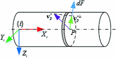

  

  Drag force on Link-i of the manipulator

  $$ \begin{aligned} \varvec{F}_{i} & = \int\limits_{0}^{{l_{i} }} {\frac{1}{2}\rho C_{D} \left\| {\varvec{v}_{P}^{r \bot } (x)} \right\|\varvec{v}_{P}^{r \bot } (x) \cdot 2r_{i} {\rm{d}}x} \quad (i = 1,2,3) \\ \varvec{N}_{i} & = \int\limits_{0}^{{l_{i} }} {\frac{1}{2}\rho C_{D} \left\| {\varvec{v}_{P}^{r \bot } (x)} \right\|(\varvec{v}_{P}^{r \bot } (x) \times \varvec{r}_{P} ) \cdot 2r_{i} {\rm{d}}x\quad } (i = 1,2,3) \\ \end{aligned} $$

  (40.8)

  where l _i is length of the i-th link and $\varvec{v}_{P}^{r \bot } (x)$ is the component of flow velocity at a point P perpendicular to the longitudinal axis. $\varvec{r}_{P}$ is the position vector of the point P relative to the origin of frame {i}. r _i is the radius of the cylinder.

40.3.1.3 Buoyancy and Gravity

Buoyancy and gravity are put together to deal with since their directions are collinear or parallel if the mass center and buoyancy center do not coincide. The resultant force $\varvec{R}_{GBi}$ and momentum $\varvec{T}_{GBi}$ of buoyancy and gravity are given as

$$ \left[ {\begin{array}{*{20}c} {\varvec{R}_{GBi} } \\ {\varvec{T}_{GBi} } \\ \end{array} } \right] = \left[ {\begin{array}{*{20}c} {\varvec{f}_{Gi} + \varvec{f}_{Bi} } \\ {\varvec{r}_{Gi} \times \varvec{f}_{Gi} + \varvec{r}_{Bi} \times \varvec{f}_{Bi} } \\ \end{array} } \right] $$

(40.9)

where f _Bi and f _Gi are the buoyancy and gravity; r _Bi and r _Gi are the position vectors of buoyancy and mass centers.

40.3.2 Inertia and Control Forces

The generalized inertia force $\varvec{R}_{i}^{*}$ and momentum $\varvec{T}_{i}^{*}$ of each body can be given as

$$ \varvec{R}_{i}^{*} = - m_{i} \cdot \varvec{a}_{i} ,\quad\varvec{T}_{i}^{*} = - {\mathbf{J}}_{i} \cdot\varvec{\alpha}_{i} -\varvec{\omega}_{i} \times {\mathbf{J}}_{i} \cdot\varvec{\omega}_{i} $$

(40.10)

where m _i represents the mass; a _i and $\varvec{\alpha}_{i}$ represents the linear and angular accelerations; J _i represents the inertia matrix.

The vehicle is driven by the propellers planted in it, which can be equivalent to being applied by a resultant force R _C0 and momentum T _C0:

$$ \varvec{R}_{C0} = \left[ {\begin{array}{*{20}c} {R_{Cx} } & {R_{Cy} } & {R_{Cz} } \\ \end{array} } \right]^{T} ,\quad\varvec{T}_{C0} = \left[ {\begin{array}{*{20}c} {T_{Cx} } & {T_{Cy} } & {T_{Cz} } \\ \end{array} } \right]^{T} $$

(40.11)

There is also a control torque T _Ci on each joint:

$$ \varvec{T}_{Ci} = {}_{i}^{0} {\mathbf{R}} \cdot \left[ {\begin{array}{*{20}c} 0 & 0 & {T_{Ci} } \\ \end{array} } \right]^{T} $$

(40.12)

where ${}_{i}^{0} {\mathbf{R}}$ is the transformation matrix from frame {0} to frame {i}.

40.3.3 Dynamic Equations

From all the concerned forces calculated, the total generalized active force and inertia force [12] can be obtained as

$$ \begin{aligned} F_{r} & = \sum\limits_{i = 0}^{4} {\left[\frac{{\partial\varvec{\omega}_{i} }}{{\partial \mathop q\limits^{.}{_{r}} }} \cdot \left(\varvec{T}_{Di} + \varvec{T}_{GBi} \right) + \frac{{\partial \varvec{v}_{i} }}{{\partial \mathop q\limits^{.}{_{r}} }} \cdot \left(\varvec{R}_{Di} + \varvec{R}_{GBi}\right )\right]} \\ & \quad + \left(\frac{{\partial \varvec{v}_{0} }}{{\partial \mathop q\limits^{.}{_{r}} }} \cdot \varvec{R}_{C0} + \frac{{\partial\varvec{\omega}_{0} }}{{\partial \mathop q\limits^{.}{_{r}} }} \cdot \varvec{T}_{C0} \right) + \sum\limits_{i = 1}^{4} {\left(\frac{{\partial\varvec{\omega}_{i} }}{{\partial \mathop q\limits^{.}{_{r}} }} - \frac{{\partial\varvec{\omega}_{i - 1} }}{{\partial \mathop q\limits^{.}{_{r} }}}\right)} \cdot \varvec{T}_{Ci} \quad (r = 1, \ldots ,10) \\ F_{r}^{*} & = \sum\limits_{i = 0}^{4} \left[\frac{{\partial\varvec{\omega}_{i} }}{{\partial \mathop q\limits^{.}{_{r}} }} \cdot\left (\varvec{R}_{Ai}^{*} + \varvec{R}_{i}^{*} \right) + \frac{{\partial \varvec{v}_{i} }}{{\partial \mathop q\limits^{.}{_{r}} }} \cdot \left(\varvec{T}_{Ai}^{*} + \varvec{T}_{i}^{*}\right)\right]\quad (r = 1, \ldots ,10) \\ \end{aligned} $$

(40.13)

According to Kane’s method, the dynamic equation of the system is established as

$$ F_{r} + { }F_{r}^{*} =0\quad (r = 1, \ldots, 10) $$

(40.14)

40.4 Simulation

Based on the dynamic equations derived previously, we perform simulations to test the stability of the vehicle at different volume ratio between the manipulator and the vehicle during the manipulator’s working process. The parameters used for the simulations are shown in Table 40.2.

Table 40.2 Parameters for simulation

We use the dimensions of the vehicle in Table 40.2 as the normal dimensions and change the volume ratio by ±10 % and ±20 %. The system is static in still water initially, and the vehicle will defect when the manipulator is moving.

The stability of the vehicle is evaluated by the Euler angle ϕ and θ. From the simulation results, as shown in Fig. 40.6, we can find that the lower the volume ratio between the manipulator and the vehicle is, the more stable the vehicle will be, and the vehicle will dip over 90° with a volume ratio bigger than 2.5 %.

Fig. 40.6

Orientation deflection of the vehicle. a Euler angle: phi, b Euler angle: theta

40.5 Conclusion

In this paper, a five-function underwater manipulator is introduced for marine salvage, underwater clearance, and other underwater tasks. A novel wrist mechanism, which uses the less inner leakage cylinder as the actuator and the groove cam for transmission, is developed for a 180° rotation. The dynamic model of the entire UVMS composed of the manipulator and a ROV are analyzed including the effects from the fluid environment for providing basic information for its control system. Dynamic simulations are performed and the results show that with a lower volume ratio between the manipulator and the vehicle, the stability of the vehicle will be higher.