
Abstract
Multivariate exponentially weighted moving average (MEWMA) control charts are widely used for detecting small mean shifts in manufacturing processes. However, the MEWMA control chart can only give out-of-control signals but provide no information on which variable or subset of variables that leads to the out-of-control signals. We propose a SVM (Support Vector Machine) based MEWMA fault identification model to help understand the underlying cause of the out-of-control signals. For each process variable, we build a SVM model for each variable to classify the out-of-control data of each variable into three classes: no mean shifts, downward mean shifts and upward mean shifts. The classification results are combined into the fault identification results. We also examine the effects of SVM parameters on classification performance and provide a SVM parameter optimization method.
This research was supported by Natural Science Foundation of China (NSFC) with grant no. 71002105.
Access provided by Autonomous University of Puebla. Download conference paper PDF
Keywords
74.1 Introduction
Statistical Process Control (SPC) is a widely used process monitoring technique for keeping processes under control. For key quality characteristics, SPC is designed to detect the evidence of whether or not there are shifts or changes (both in the process mean and variance) in manufacturing processes with proper sampling scheme.
In complex products manufacturing processes, it is quite common to simultaneously monitor several correlated quality characteristics. MSPC (Multivariate statistical process control) chart was proposed to monitor process with more than one correlated variables. The T 2 control chart was put forward by Hotelling (1947). It was tested that the T 2 chart is insensitive to minor shifts (Lowry et al. 1992). Thus the EWMA (Exponentially weighted moving average) and CUSUM (Cumulative Sum) charts were extended to multivariate process monitoring scenarios. The MCUSUM chart was introduced by Woodall and Ncube (1985), Healy (1987), Crosier (1988), Pignatiello and Runger (1990). The MEWMA chart was studied by Reynolds and Kim (2005), Zou and Tsung (2008).
With the application of computer technology in manufacturing processes and the enhancement of data collection technology, machine learning and data mining techniques have been used in multivariate process monitoring and fault identification. The artificial neural network (ANN) has been used as an effective tool for detecting the deviation of mean and/or covariance matrix in manufacturing processes (Guh 2007; Niaki et al. 2005; Wang and Chen 2002). Other related methods also have been used, such as the combination of ANN and Rough Set (RS) (Hou et al. 2003) and the combination of ANN and Genetic Algorithm (GA) (Yu and Xi 2009; Yu et al. 2008). A comparison of Support Vector Machine (SVM) and ANN for drug/nondrug classification has been done by Byvatov et al. (2003) and it was demonstrated that the SVM system used in the study has capacity to produce higher overall prediction accuracy than a particular ANN architecture.
In this paper we propose a SVM based model for fault identification in MEWMA control charts. The rest of this paper is organized as six sections. In the next section, a SVM-based MEWMA control fault identification model is introduced. Followed by the model training and testing results with scenarios of p = 2. Then we also examine the effects of two SVM parameters on the performance of MEWMA fault identification. Finally a summary on the paper is presented.
74.2 Methodology
There are two main modules in the SVM-based MEWMA fault identification model:
-
(1)
Process monitoring. Firstly, we can estimate the process parameters, mean vector and variance–covariance matrix, using the collected historical process quality data (If the process parameters are all known, this step can be omitted). Then we can construct the MEWMA control chart based on the estimated parameters.
-
(2)
Model training and testing. Using the estimated process parameters, we can generate random data with designed mean shift patterns. Then we can train and test the SVM model using the generated data. When there are out-of-control signals in the MEWMA control chart, the data are imported into the trained model. The output of the model will be the fault identification results which can be used to remove the fault in the manufacturing processes.
In the procedure of model training and testing, we must design different mean shift patterns. For each variable, we study three kinds of conditions, i.e. no mean shifts, mean shifts downwardly and mean shifts upwardly. For a process with p quality variables, there are totally 3p combinations include one in-control combination and 3p-1 out-of-control combinations. With the increase of p, the number of such combinations increases exponentially. We proposed a SVM-based MEWMA fault identification model here (see Fig. 74.1).
Fig. 74.1 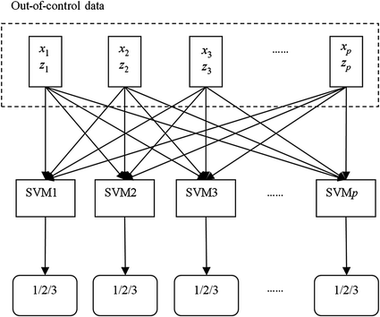
A proposed SVM-based MEWMA fault identification model
In the proposed model, we diagnose the variables independently. There are three kinds of outputs of each SVM, i.e. 1, 2 and 3. If there are no mean shifts in a variable, the output of the related SVM should be 1; if the mean of a variable shifts downwardly the output of the related SVM should be 2. The output of a SVM should be 3 if the mean of the related variable shifts upwardly. The number of SVM equals to the number of variables and the difficulties in model building is linear to the number of variables. Compared to the models reported by Guh1 and Yu & Xi5 in which the number of the classes of the output is 3p, the advantage of the proposed model is that the model building is much easier when p is large.

74.3 SVM Training and Testing
The proposed model is built based on four assumptions. First, we assume that we can accurately estimate the mean vector and variance–covariance matrix of the process data given enough data. Second, there will only be mean shifts in the process while the variance–covariance matrix remains constant. Third, only abrupt shifts are considered here, which means that the data before and after shifts are all independently and identically distributed. Lastly, a process is assumed to remain in-control until a mean shift occurs. The shift will change the parameter estimation of the process data. We also assume that an out-of-control process will not become in-control until faults are found and removed.
74.3.1 Training and Testing Data Generation
Let \( {\varvec{\upmu}}_{ 0} \) be the in-control process mean vector and \( {\varvec{\Upsigma}}{}_{0} \) the in-control process variance–covariance matrix. A MEWMA control chart can be built if both parameters are known. The selection of smoothing factor and control limit of such a control chart is reported by Lowry et al. (Guh 2007). For presenting the interesting mean shifts intervals, we set the mean shift coefficients (k 1, k 2, …, k p ) to be the values of (−3.0, −2.0, −1.0, 0.0, 1.0, 2.0, 3.0). For a process with p variables, there are 7p combinations include one in-control combination and 7p−1 out-of-control combinations, denoted by M. We generated a set of random data using the multivariate normal random data generation function mvnrnd(.,.) in Matlab®. There were N 1 in-control samples and N 2 out-of-control samples in the generated data set. The data generation procedure is described as follows.
-
(1)
Set i = 1 and generate N 1 in-control data.
-
(2)
Generate out-of-control data X with a shifted mean vector. \( {\varvec{\upmu}}_{ 0} + \Updelta {\varvec{\upmu}} \), where \( \Updelta {\varvec{\upmu}} = \left( {k_{i1} \sigma_{1} ,k_{i2} \sigma_{2} , \ldots ,k_{ip} \sigma_{p} } \right),k_{ij} ,i = 1,2, \ldots ,M;j = 1,2, \ldots ,p \) is the ith mean shift coefficient of the jth variable, and \( \sigma_{i} ,i = 1,2, \ldots ,p, \) is the standard deviation of the jth variable. The statistics Z and T 2 are calculated for each sample.
-
(3)
Z is compared to the MEWMA control limits. If it is outsides the control limits, both X and Z are recorded.
Go to step 3 if the number of X is less than N 2, otherwise, set i = i + 1 and return to step 1.
For model testing, the mean shift coefficients are set to the values of (0.00, −1.15, −1.35, −1.55, −1.75, −2.25, −2.65, −2.85, −3.05, −3.25, 1.15, 1.35, 1.55, 1.75, 2.25, 2.45, 2.65, 2.85, 3.05, 3.25). The testing data are also generated using the above procedure.
74.3.2 SVM Parameters Selection
In this section we aim to determine the optimal SVM parameter values. To do that, we fix the process parameters and examine the effect of the SVM parameters on the performance of the proposed model. We consider an in-control process with \( {\varvec{\upmu}}_{ 0} = [0 \, 0] \) and \( {\varvec{\Upsigma}}_{0} = \left[ {\begin{array}{*{20}c} 1 & {0.5} \\ {0.5} & 1 \\ \end{array} } \right] \). and set the number of in-control samples (N 1) to be 100. To build a SVM model, we construct a vector V = [X Z d], where X is the raw data, Z is the MEWMA statistic of X and d is the classification label. We follow Lowry et al.’s suggestion (1992) that the smoothing coefficient of the MEWMA control and control limit h should be set to 0.1 and 8.66, respectively. The number of samples considered for each mean shift combination (N 2) is set to be 30.
As we discussed earlier, we use the Gaussian radial basis function as the SVM kernel function. There are two important parameters in the SVM model; including the penalty factor C and kernel function parameter b 2. We analyze the effects of these two parameters on the performance of our SVM models for fault identification with an example with two variables, i.e. p = 2. We select C = 100, 1,000, and 10,000, the values of b 2 are set to be in the range between 0.5 and 14.9 with an increment of 0.3. The correct ratio of both SVM1 and SVM2 are analyzed for the model training and testing. The testing results are presented in Fig. 74.2.

The SVM training and testing performance with C = 1000 and 10,000
Figure 74.2 illustrates the performance of SVM for C = 100, 1,000, and 10,000. For each value of C, with the increase of b 2 the correct ratio values increase obviously and then reach the max value. After that the correct ratio values decrease slightly. And the correct ratio values with C = 1,000 and C = 10,000 are nearly the same when b 2 is greater than 5.
74.3.3 SVM Training and Testing Results
After choosing the optimal SVM parameters, we analyzed the performance of SVM training and testing given different correlation coefficients (ρ). We let the correlation coefficient be one of the following values (0.1, 0.3, 0.5, 0.7, 0.9). The SVM parameters are set to be C = 10,000 and b 2 = 10.4. We run the simulations for 1,000 times to each correlation coefficient value and the results are presented in Table 74.1. The correct ratios are also depicted in Fig. 74.3. It shows that the correlation coefficient do have effects on the performance of the SVM-based MEWMA fault identification model. When the correlation coefficient increases, the correct ratios of the SVM training decrease accordingly. The correct ratio of SVM1 training decreased from 94.22 % (ρ = 0.1) to 91.72 % (ρ = 0.9). The correct ratio of SVM2 training decreased from 94.33 % (ρ = 0.1) to 91.72 % (ρ = 0.9). Considering both SVM1 and SVM2, the overall correct ratio decreased from 88.57 % (ρ = 0.1) to 84.38 % (ρ = 0.9).

Variances of SVM training and testing with different correlation coefficients
However, the correct ratio increases in the model testing while the correlation coefficient increased. The correct ratio of SVM1 testing increased from 92.99 % (ρ = 0.1) to 95.46 % (ρ = 0.9). The correct ratio of SVM2 testing increased from 93.03 % (ρ = 0.1) to 95.42 % (ρ = 0.9). Considering both SVM1 and SVM2, the overall correct ratio increased from 86.18 to 91.21 %. The average testing correct ratio was 88.57 %. Although the proposed approach achieved the highest correct ratio when the correlation coefficient was the highest, its performance is still acceptable when the correlation coefficient is small.
Furthermore, most of the variances in both training and testing results were relatively small. It shows that the performance of our model is stable under different conditions.
74.4 Summary
We proposed a MEWMA control charts fault identification model using SVM which is built on the concept of SRM. SVM has minor generalization errors compared to the approaches based on the concept of least-squares or maximum likelihood. After a brief introduction of MEWMA control charts and SVM, we gave an SVM-based model for MEWMA control chart fault identification when there are out-of-control signals in control charts. The raw process data X and the MEWMA of X are set as the input of the model and the process variables are diagnosed independently and this can reduce the difficulties of model building when the dimension of the problem increased.
References
Byvatov E, Fechner U, Sadowski J, Schneider G (2003) Comparison of support vector machine and artificial neural network systems for drug/nondrug classification. J Chem Inf Comput Sci 43(6):1882–1889
Guh RS (2007) On-line identification and quantification of mean shifts in bivariate processes using a neural network-based approach. Qual Reliab Eng Int 23:367–385
Healy JD (1987) A note on multivariate CUSUM procedures. Technometrics 29(4):409–412
Hotelling HH (1947) Multivariate quality control. In: Eisenhart C, Hastay MW, Wallis WA (eds) Techniques of statistical analysis. McGraw-Hill Professional, New York
Hou TH, Liu W-l, Lin L (2003) Intelligent remote monitoring and diagnosis of manufacturing processes using an integrated approach of neural networks and rough sets. J Intell Manuf 14(2):239–253
Lowry CA, Woodall WH, Champ CW, Rigdon SE (1992) A multivariate exponentially weighted moving average control chart. Technometrics 34(1):46–53
Niaki STA, Taghi S, Niaki A, Abbasi B (2005) Fault diagnosis in multivariate control charts using artificial neural networks. Qual Reliab Eng Int 21(8):825–840
Pignatiello JJ, Runger GC (1990) Comparisons of multivariate CUSUM charts. J Qual Technol 22(3):173–186
Reynolds MR, Kim K (2005) Multivariate monitoring of the process mean vector with sequential sampling. J Qual Technol 37(2):149–162
Wang TY, Chen LH (2002) Mean shifts detection and classification in multivariate process: a neural-fuzzy approach. J Intell Manuf 13(3):211–221
Woodall WH, Ncube MM (1985) Multivariate CUSUM quality-control procedures. Technometrics 27(3):285–292
Yu JB, Xi LF (2009) A neural network ensemble-based model for on-line monitoring and diagnosis of out-of-control signals in multivariate manufacturing processes. Expert Syst Appl 36(1):909–921
Yu JB, Xi LF, Zhou X (2008) Intelligent monitoring and diagnosis of manufacturing processes using an integrated approach of KBANN and GA. Comput Ind 59(5):489–501
Zou CL, Tsung FG (2008) Directional MEWMA schemes for multistage process monitoring and diagnosis. J Qual Technol 40(4):407–427
Author information
Authors and Affiliations
Corresponding author
Editor information
Editors and Affiliations
Rights and permissions
Copyright information
© 2013 Springer-Verlag Berlin Heidelberg
About this paper
Cite this paper
Li, L., Jia, H. (2013). On Fault Identification of MEWMA Control Charts Using Support Vector Machine Models. In: Qi, E., Shen, J., Dou, R. (eds) International Asia Conference on Industrial Engineering and Management Innovation (IEMI2012) Proceedings. Springer, Berlin, Heidelberg. https://doi.org/10.1007/978-3-642-38445-5_74
Download citation
DOI: https://doi.org/10.1007/978-3-642-38445-5_74
Published:
Publisher Name: Springer, Berlin, Heidelberg
Print ISBN: 978-3-642-38444-8
Online ISBN: 978-3-642-38445-5
eBook Packages: EngineeringEngineering (R0)