
Abstract
Back-scattered Scanning Electron Microscopy (BSEM) has been used to identify weathering mechanisms occurring in two oolitic limestones from urban areas in London and Cambridge, United Kingdom. From a petrographical point of view, the two stones can be described as oosparite and oomicrite, their main distinctive feature being the crystal size of the cement binding the limestone grains together. The sulphation mechanism, i.e. the replacement of calcium carbonate (calcite: CaCO3) by calcium sulphate dehydrate (gypsum: CaSO4 2H2O), at the surface and within the stone fabric is confirmed as the general decay process. Differences in macroporosity/permeability distribution in the two limestones lead to different weathering patterns. BSEM provides evidence that gypsum patinas still commonly found on limestone facades in polluted urban locations are advancing inside the diseased stone and that their removal is urgently needed to arrest the growth of the in-growing weathering front.
Access provided by Autonomous University of Puebla. Download chapter PDF
Keywords
These keywords were added by machine and not by the authors. This process is experimental and the keywords may be updated as the learning algorithm improves.
6.1 The Application of Back-Scattered Scanning Electron Microscopy to Unravel Building Stone Decay Mechanisms in Urban Environments
Abstract Back-scattered Scanning Electron Microscopy (BSEM) has been used to identify weathering mechanisms occurring in two oolitic limestones from urban areas in London and Cambridge, United Kingdom. From a petrographical point of view, the two stones can be described as oosparite and oomicrite, their main distinctive feature being the crystal size of the cement binding the limestone grains together. The sulphation mechanism, i.e. the replacement of calcium carbonate (calcite: CaCO3) by calcium sulphate dehydrate (gypsum: CaSO4 2H2O), at the surface and within the stone fabric is confirmed as the general decay process. Differences in macroporosity/permeability distribution in the two limestones lead to different weathering patterns. BSEM provides evidence that gypsum patinas still commonly found on limestone facades in polluted urban locations are advancing inside the diseased stone and that their removal is urgently needed to arrest the growth of the in-growing weathering front.
6.1.1 Introduction
Rising levels of air pollution in modern urban agglomerates not only have deleterious effects on human health but may also be correlated with the onset of serious decay patterns on a variety of earth materials used in built heritage monuments. Stone is no exception. One of the most commonly used lithotypes is limestone, a high porosity sedimentary rock composed of a framework of grains (minerals, fossils and, as in the case illustrated in this chapter, ooids) bound together by a “cement” of calcium carbonate crystals (i.e. calcite: CaCO3) either fine (<5 μm—micrite) or coarse grained (>5 μm—sparite). Ooids (also named oolites) are spherical or ellipsoidal grains which have regular concentric laminae of fine-grained carbonate developed around a nucleus, usually a quartz grain. Through laboratory and field based studies, studies focusing on the decay of limestones in polluted urban environments have highlighted the importance of the sulphating mechanism, by which atmospheric SO2, released mainly by the combustion of fossil fuels such as coal and oil, in reacting with the stone’s CaCO3 promotes the growth of decay-inducing sulphate patinas [1–7]. Despite the recent implementation of environmental laws setting strict limits to SO2 levels in urban areas [8], which has now resulted in a significant reduction of SO2 emissions in today’s urban environments, gypsum patinas are still disfiguring building façades in several major European towns especially where high-sulphur coal had been extensively used in the past such it is the case in the UK [2, 7, 9] and Eastern Europe [10].
The growth of black gypsum-rich crusts on the stone surface in areas sheltered from episodes of rain wash-outs is therefore a well-known and still active phenomenon. However, the detailed growth mechanism and related chemical weathering pathways correlated with these patinas are still the subject of some debate. With regards to the progression of the weathering front inside the stone, for instance, some researchers suggest that gypsum crystals replacing calcite now seen at the outermost crust–atmosphere interface are the “oldest”, i.e. the ones precipitated first. Others noted that that the distribution of aerosol particulate matter derived from fossil fuel burning imbedded within gypsum patinas seems to record an outward growth of the crusts during historic changes in urban pollution sources [2, 4, 11, 12]. Indeed, a “stratigraphical” pattern in the distribution of particulate pollutants in particularly thick gypsum crusts from central London (Westmister Palace) has been recognised [12]: in these studies, particles from historical coal burning activities were found concentrated close to the innermost crust–stone interface while particles typical of “recent” oil burning sources were most common near the outermost crust–atmosphere interface. This stratigraphical distribution, while supportive of the outward growth hypothesis, is, however, by no means present in all samples of black crusts from monument façades in urban areas. The scientific debate regarding the inward versus outward crust growth mechanism is of no trivial nature as it relates directly to a conservation open issue between conservators advocating a protective role of these crusts against further attack by environmental agents and those who strongly advise their prompt removal by different cleaning methods (wet chemical and/or laser assisted).
In this chapter, we examine the application of Scanning Electron Microscopy (SEM) interfaced with Energy Dispersive X-ray Spectroscopy (EDS) to examine the urban weathering behaviour of oolitic limestones in two British monuments (Fig. 6.1): King’s College Chapel, Cambridge and St. Luke’s Church, Chelsea, London. The SEM is used here in back-scattered mode (BSEM). BSEM is particularly useful in the examination of thin sections spanning the weathering patina–stone substrate interface as in this mode the brightness of individual mineral phases under SEM is directly correlated with the average atomic number of the elements forming the chemical composition of the same phases: in other words, the heavier the elemental composition of the mineral under view (for example Fe-containing minerals) the brighter the image in the SEM monitor.

King’ College Chapel, Cambridge (left) and St. Luke’s Church, Chelsea, London (right)
Aim of this BSEM study was threefold: (a) assess the role played by petrographical differences in pollution-derived decay of apparently similar building limestones; (b) compare the relative soundness of two limestone lithologies subjected to different levels of past and present air pollution (Cambridge vs. London); (c) further investigate the detailed growth mechanisms of gypsum weathering patinas on limestone.
6.1.2 Petrographical Notes and Methodology
Both monuments are built in oolitic limestone. The main petrographical difference between the two limestones is the type of cement binding the constituent grains together: in the King’s College stone, the cement is mainly composed of microcrystalline calcite (oomicrite) whereas in the St. Luke’s stone the cement is largely composed of large interlocking calcite crystals (oosparite). Oolitic limestones, at least in the Cambridge case [13] were probably chosen because of their high degree of original cementation as both limestones show postdepositional features (such as interpenetrating grain boundaries) suggesting that they were subjected to considerable compaction during their geological history.
Polished surfaces of the samples were sputter-coated with gold and then examined with a JEOL 820L SEM interfaced with LINK system AN10000 EDS microanalysis system.
6.1.3 BSEM Observations
In both monuments, decay leads to the built-up of gypsum crusts of variable thickness (up to 1 cm). Thicker crusts in the London samples probably correlate with higher degrees of atmospheric pollution. Apart from gypsum crystals, other constituents include anthropogenic particles, calcite, silicate particles (quartz and feldspar) and fossil fragments. In particular, anhedral (i.e. with a not well-formed crystal habit) calcite grains are very common and evenly distributed throughout the crusts. Continuous calcite horizons are also present. Fossil grains can often be seen even near the crust–atmosphere interface. Aerosol particles from fossil fuel burning activities do sometimes show a “stratigraphic” distribution with a higher number of oil derived (i.e. recent pollution) carbonaceous particles at the outer edge and coal derived (i.e. historic pollution) aluminosilicate spherical particles (together with wood fragments) closer to the stone substrate interface. A typical feature within gypsum patinas is the presence of ooid “ghosts”, i.e. areas now completely filled with acicular gypsum crystals still retaining a faint spherical oolitic outline (Fig. 6.2). These areas are free of imbedded particles and clearly represent areas formerly occupied by the stone substrate prior to sulphate attack.

St. Luke’s Church. Former calcite oolite being replaced by gypsum. Some oolitic layers and nucleus still calcitic. Oolitic layered texture preserved
Despite these apparent similarities, detailed BSEM investigation reveals how atmospheric chemical attack progressed differently in two building stones examined.
6.1.3.1 St. Luke’s Church
The sulphation weathering front starts at the stone–crust interface and may reach a depth of several centimetres inside the stone. Calcitic oolites have been and are presently undergoing gypsum replacement. The preservation of calcitic remnants and the lower S content (as revealed by EDS analysis) at the centre of the oolites suggests that the replacement occurs from the outer edges of the oolites towards the centre (Fig. 6.2). The original ooid texture is commonly preserved suggesting that the gypsum replacement is a slow replacive process not always involving previous dissolution of the calcite with an intervening void phase before gypsum precipitation. In some cases, however, the typical oolitic texture is destroyed although the spherical outline of the ooid is still visible. Occasionally, the space previously occupied by the ooid is now filled with anthropogenic particles and mineral fragments. The sulphation also affects the sparite cement but not through a replacement process: gypsum instead crystallises within fractures and cleavage planes splitting calcite crystals apart; detached calcite fragments are slowly incorporated into the growing crust (Fig 6.3).

St. Luke’s Church: stone–crust interface. Gypsum crystals (G) crystallising within cleavage planes and intercrystalline boundaries split calcite cement into fragments (C) which are then incorporated into the growing crust. Anthropogenic particles from fossil fuel burning are also present (red arrows)
6.1.3.2 King’s College Chapel
Most of the oolites in Kings Chapel weathered stone samples, in contrast with St. Luke’s ones, do not show extensive gypsum replacement, although crystallisation of gypsum within ooid laminae and microfractures has been observed (Figs. 6.4, 6.5, 6.6). The micritic cement is, however, almost completely replaced by acicular gypsum crystals up to a depth of several centimetres underneath the current stone–crust interface (Fig. 6.4). Authigenic dog-toothed calcite is also seen precipitating at the oolite edges as a fringe cement (Fig. 6.6). This type of decay may deceitfully lead to an overestimation of the stone soundness because of the apparent high degree of cementation. Widespread sulphation of the cement can also be seen in areas of the stone where exposure to episodes of rain wash-outs have prevented the development of fully grown gypsum patinas. The net effect of sulphation is a sharp increase in intergranular porosity: a fragile framework of oolite grains with intervening void spaces is thus created. Macroscopically, this leads to superficial crumbling of the stone into a fine “oolitic” powder and to a complete loss of cohesion. In many instances, a band of clear gypsum crystal (i.e. with no imbedded anthropogenic and/or soil dust particulate matter) is present near the stone–crust interface (Fig. 6.5).

King’s College Chapel. Secondary acicular gypsum crystals precipitate within the pore spaces after dissolution of the original micrite cement. Stone porosity increases

King’s College Chapel. Extensive areas of gypsum/replacement crystallisation (G) of micrtic cement (C) occur deep inside the stone fabric. Incipient oolite replacement is also present (arrows)

King’s College Chapel. Close-up of secondary acicular gypsum cement, showing also the reprecipitation of dog-toothed calcite as a fringe cement around oolitic grains as well as the detachment of layers of oolitic cortex due to gypsum crystallisation pressures (arrows)
6.1.4 Discussion and Decay Model
The ubiquitous presence of authigenic gypsum at the surface and within the pore spaces of the studied oolitic limestones confirms sulphation as the main decay process. The BSEM examination suggests that the following decay mechanisms have affected the building stones. Atmospheric pollutants, namely SO2, are adsorbed on the stone surface either by wet or dry deposition. Wetting of the stone cause sulphation to begin and calcite starts to get replaced by gypsum. Weathering solutions penetrate within the stone along cracks and intercrystalline boundary planes. At this stage, differences in stone microtexture lead to different decay patterns (Fig. 6.7).

Decay
Oosparite (St. Luke’s Church-London). The oolitic grains are preferentially replaced with respect to the cement. The mechanism of replacement my follow one of two routes: (i) dissolution of the calcite followed by precipitation of gypsum in the void thus created; (ii) slower atom by atom replacement via a thin film mechanism similar to that reported for the transformation of the mineral aragonite (CaCO3) into its polymorph (i.e. same chemistry, different crystalline structure) calcite [14]. The preservation of laminae within the cortex of many ooids (Fig. 6.2) would suggest the second mechanism to be predominant although episodes of dissolution and void creation are present. Gypsum crystals precipitating within cleavage planes and intercrystalline boundaries of calcite cement crystals results in their fragmentation (Fig. 6.3). Incorporation of these crystalline fragments into the growing crust is clearly visible and suggests that most of the anhedral calcite imbedded within the crust are not soil dust but remnants of the desegregated cement.
Oomicrite (King’s College-Cambridge). Most of the oolite grains are still calcitic whereas the microcrystalline cement (micrite), despite its low permeability, is almost completely replaced by gypsum (Fig. 6.4). The replacement process is likely, in this case, to have involved early dissolution of the fine-grained micrite as suggested by the presence of intergranular microcavities in areas not yet subjected to sulphation. Microsplitting of ooid laminae due to gypsum growth is present but, in this case, does not greatly affect the overall stone soundness (Fig. 6.5).
Differences in micropore distributions between cement and ooid grains in oosparite and oomicrite are responsible for the observed selective replacement features. Limestone porosity studies indicate that in oosparites the microporosity is mainly located within ooid grains whereas in oomicrites, most of the interconnecting pores, affecting stone permeability are located within the micritic cement. The smaller crystal size of the micrite cement in King’s College samples offers a greater specific area for chemical attack explaining why micrite is more easily replaced than large sparite calcite crystals. The fact that most of the ooid grains are still composed of calcite might also reflect the lower degree of SO2 air pollution in Cambridge as opposed to London. The dissolution/replacement of micrite is probably occurring at a fairly early stage in the decay process: further decay would probably result in the in the replacement of ooids as seen in St. Luke’s samples. In both examples, the presence of gypsum filled “ghosts” within the crusts near the stone–crust interface provides clear evidence that the chemically active weathering occurs inside the limestone and that crusts grow in thickness mainly at the expense of the stone substrate. Gypsum crystals get “younger” in an inward direction.
6.1.5 Conclusions
Compared to standard Optical Microscopy, BSEM is a useful tool in the investigation of building stone surface weathering in urban environments due to its higher magnification, higher lateral resolution and “instant” phase information based on changes in image brightness between minerals containing elements of various atomic numbers. In the case study illustrated in this chapter, for instance, the technique revealed slightly different decay pathways in the two similar but distinct lithological types examined. In oosparites, the main cause of decay is crystallisation pressures arising from gypsum crustallisation within cleavage planes and intercrystalline boundaries of the sparitic cement. In oomicrites, the main cause of decay is the dissolution of secondary gypsum cement replacing the original micrite.
In conservation terms, the oosparite seems to provide a better resistance to decay. The growth of gypsum crusts occurs in both directions, inwards and outwards, with respect to the original stone surface. The predominant direction is towards the interior of the stone, though, highlighting the need for an urgent removal of the patinas followed by the application of stone consolidants and water repellents.
6.2 Application of Microscopy, X-ray Diffractometry (XRD) and Stable-Isotope Geochemistry in Provenance Determination of the White Marbles Used in the Ancient Great Theatre of Larisa, Thessaly, Greece
Abstract The present work aims in identifying the exact source of the marbles used in the koilon from the ancient Great Theatre of Larisa, for maintenance purposes. Emphasis is given on the C–O isotopes of marble (δ13C = +2.62 to +2.93 ‰ and δ18O = −4.75 to −5.78 ‰). Mineralogical and petrographical investigations further refine the marble characteristics. Based on the comparison with seven different quarrying sites in Thessaly, it is concluded that the marble for the construction of the theatre was from the Kastri quarries.
6.2.1 Introduction
The Great Theatre of Larisa is one of the biggest well-preserved ancient theatres of Greece, totally built by stone. It was constructed in the beginning of the third century BC based on the Classical architecture [15, 16]. It consists of three major parts: the Scene, the Orchestra and the Koilon, a semicircular area of stepping seats, comprising the main part of the theatre. Koilon was built by fine-quality white-marble blocks. Fourteen series of seats are still preserved (Fig. 6.8), whereas the higher part (epitheatron) has been mostly removed or covered by modern buildings [15]. During the second century BC, a Doric style proscenium was added in front of the scene. Between the second and the first century BC, the theatre was subjected to extensive reconstructions due to a partial destruction attributed to a seismic event [17]. The Great Theatre was in use until the end of the third century A.D., when was probably flooded by the sediments of Pinios river which flows only 200 m to the West [18].

Map of Thessaly in central Greece, showing the location of the ancient Great Theatre in Larisa (small photograph at the upper left corner) and the ancient white-marble quarrying sites: 1. Tisaion mount (ancient Atrax), 2. Olympos mount (ancient Gonnoi), 3. Ossa mount (Tempi), 4. Chasanbali, 5. Kalochori, 6. Mavrovounion mount (Kastri) and 7. Magnesia–Tisaion mount
The first works for unearthing the theatre started in 1910, but the large revelation of the monument was due to the broader excavation programme between 1985 and 2000, by the fifteenth Ephorate of Prehistoric and Classical Antiquities, directed by Tziafalias. Today, a large project focusing on the preservation and restoration of the koilon is in process. The main problems are concentrated in damages, such as displacements and breaks of the large marble blocks, attributed to strong earthquakes [18]. For the maintenance purposes, it is of critical importance for the archaeologists to know the precise quarries in order to replace the broken and damaged slabs from the same quality marble with equivalent features.
The present work aims in identifying the exact ancient source of the marbles used in the koilon from the Great Theatre of Larisa, through a mineralogical, petrographical and isotopic study. In fact, the provenance studies contribute in the location of the best materials for restoration, but also offer valuable information in the ancient trading and communication routes during ancient times.
6.2.2 Sampling and Methodology
A total of six marble samples (AThL1-6) were collected from the koilon of the ancient theatre, especially from the main part, apart from one sample which is from the upper section, the epitheatron. It should be mentioned that all the samples were detached from hidden broken parts of damaged seats and they do not exceed 2 × 2 × 1 cm in dimensions.
From each sample, a thin section was prepared for the purpose of mineralogical and petrographical study by polarising microscopy at the Department of Mineralogy-Petrology-Economic Geology, Aristotle University of Thessaloniki (AUTh). Microscopy was employed to determine the fabric of the mineral constituents, with particular reference to calcite, as well as to detect the frequency and distribution of the accessory grains. The maximum grain size (MGS) of calcites and the geometric relationships of the carbonate grains, such as the grain boundary shape, were also evaluated.
In addition, powders of the samples were processed by X-ray diffraction (XRD) in order to distinguish calcite from dolomite and to verify the related abundances in each sample. The XRD analyses were performed at the Department of Mineralogy-Petrology-Economic Geology, AUTh, with a PHILIPS PW1710 diffractometer (Ni-filtered CuKα/Ni: 40 kV, 0.01° 2θ, 3–63°, 0.02° 2θ/s).
Oxygen and carbon isotope analyses of the marble samples were carried out at the Department of Earth Sciences, Royal Holloway University of London. The oxygen and carbon isotope ratios are referred to the standard VDPB (Belemnitella americana from the Cretaceous Pee Dee Formation, South Carolina).
The applied methods have been successively used so far by many researchers, such as Coleman and Walker [19], Herz [20], Herrmann et al. [21], Capedri and Venturelli [22], Maniatis et al. [23, 24] and Al-Naddaf [25], for the source identification of ancient marble artefacts.
This study is based on the documentation of the ancient white-marble quarries of Thessaly, the development of well-defined data-bases with mineralogical, petrographical and oxygen and carbon isotope ratios, and the statistical treatment of the measured parameters. Previous works from Germann et al. [26], Capedri et al. [27], Melfos [28] and Melfos et al. [29] have defined the geological and isotopic characteristics of the marbles at seven ancient quarrying sites in Thessaly, located: at Titanos mountain (ancient Atrax), at Olympos mountain (ancient Gonnoi), at Ossa mountain (Tempi), at Mavrovouni mountain (Kastri), at Kalochori and Chasanbali, nearby the famous quarries of the ophicalcitic Green Thessalian stone [30], and at Tisaion mountain in Magnesia (Fig. 6.8). The mineralogical composition, the textural features, the MGS and a brief description of the marbles from each ancient quarry are depicted in Table 6.1, which also reports O and C isotope compositions.
6.2.3 Results
All the marble samples from the ancient theatre have a white colour and they are coarse grained, with visible calcite crystals. In some cases, grey-green coloured thin orientated stripes are observed parallel to the schistosity. The XRD analyses and the microscopic investigation showed that the mineralogical composition remains almost the same in the whole sample suite and consists mainly of calcite, with dolomite quartz, white mica, opaque minerals (sulphides) and Fe-oxides as accessory minerals. Traces of chlorite, when observed, are related to the grey-green orientated stripes.
The maximum grain size (MGS), a diagnostic feature for discriminating marbles, is 5–6 mm. This MGS is typical of the coarse-grained marbles from different localities in Thessaly, such as Gonnoi, Tempi and Kastri (Table 6.1). The marble samples exhibit a heteroblastic texture with small grains, up to 500 μm in diameter, coexisting with larger crystals with a size reaching 6 mm, and only occasionally they show a homeoblastic texture. This is typical of Atrax, Kalochori and Kastri marbles (Table 6.1). In some samples (AThL3, AThL4, AThL5), the marble is characterised by a high degree of preferred orientation of the calcite crystals which are considerably distorted by elongation, flattening and bending as a result of intensive strain. This fabric has been observed in some cases in marbles from Tempi and Kastri (Table 6.1). The shape of the grain boarders is sutured to dentate and frequently embayed (e.g. grains are interlocked) indicating non-equilibrated metamorphic conditions.
All the samples contain small flakes of white mica and rounded quartz grains with a length up to 1 mm. Chlorite flakes with a maximum size 500 μm were observed in one only sample. Opaque minerals (probably sulphides) are seldom found among the calcite crystals and their size does not exceed 5 μm. This mineralogical composition resembles the Kastri and partly the Gonnoi marbles.
The C–O isotopic results of the marble samples from the ancient theatre are plotted in the diagram of Fig. 6.9. The δ13C values range from +2.62 to +2.93 ‰ and the δ18O values from −4.75 to −5.78 ‰. It is obvious that these values have a consistent signature and in the diagram of Fig. 6.9 they plot in a restricted field. Reference isotopic fields of the marbles from the ancient quarries in Thessaly are also shown in the same diagram.

A δ18O–δ13C diagram for the archaeological marble samples from the ancient Great Theatre of Larisa. Reference isotopic fields of the marbles from the ancient quarries in Thessaly are also shown: Kalochori, Kastri, Gonnoi, Atrax, Tisaion, Tempi, Atrax and Ghasanbali, published by Germann et al. [26], Capedri et al. [27], Melfos [28] and Melfos et al. [29]
6.2.4 Discussion
The microscopic investigation, the XRD and the stable-isotope analyses of six marble samples from the ancient Great Theatre of Larisa demonstrate consistent results with regard to the mineralogical composition, the petrographical features and mainly the C–O isotope ratios (Fig. 6.9).
Especially, the isotopic ratios of C and O provide usable signatures for determining the provenance of marbles. Isotopic analyses involve measuring of the 13C/12C and 18O/16O ratios in marble and the results are expressed in terms of the deviation from a conventional standard. This deviation, called δ, is expressed as δ13C and δ18Ο in parts per thousand (% or per mil) and forms the isotopic signature. The values exhibit a relatively restricted range in each quarry area or limited parts of a geological formation [31, 32]. On the δ13C–δ18O correlation diagram, the geological samples of the marbles fall into well-defined groups and each quarrying site is therefore discriminated.
Comparing the isotopic results of the studied marbles from the theatre with the marbles from the Thessalian ancient quarries, it is evident that they plot in the groups of Tempi and Kastri and partly of Chasanbali marbles (Fig. 6.9). Consequently, all the other quarries are excluded as possible sources.
Based on mineralogical and petrographical features, discrimination among the possible sources (Tempi, Kastri or Chasanbali) is possible. The marble in Tempi consists only of calcite and its texture is mostly homeoblastic. The marble in Chasanbali contains calcite and quartz and is fine grained with homeoblastic texture. In contrast, the marbles from the theatre are made of calcite with traces of dolomite, white mica, quartz, opaque minerals, Fe-oxides and rarely chlorite and have a coarse-grained heteroblastic texture. Therefore both quarrying sites, Tempi and Chasanbali, are also excluded as possible marble sources for the theatre of Larisa. In addition the white-marble quarry in Chasanbali is small and unimportant and could not provide such a large amount of raw materials for the theatre construction.
Mineralogical composition obtained by XRD and microscopy showed that the Kastri marble is almost identical with the whole suite of the eleven studied marbles from the theatre. The textural features have also significant similarities being mainly coarse-grained heteroblastic, and in some cases elongated calcite crystals are observed. The large MGS, in the case of Kastri and the marbles from the theatre, are 5–6 mm.
It is evident that only the Kastri marble quarry demonstrates similar mineralogical and isotopic features with the studied marbles and shows that it is the most probable source for the marbles of the Great Theatre of Larisa (Fig. 6.8).
6.3 Case Studies: Investigation of Mortars by Infrared and Raman Spectroscopy
Abstract Infrared (IR) and Raman spectroscopy permit the identification of X-ray amorphous minerals. Mechanisms of material decay and principles of cause and effect can be elucidated. We discus three examples: (i) decay due to alkaline-rich mortar, (ii) effect of nitrate-rich mortar, (iii) identification of historic mortar. Damages to historic buildings may not only be caused by their actual utilisation or by contemporary pollutants. Natural influences acting for centuries even without any human interference may have put deteriorating strain on a historic structure as well. The impact of such strains rises if inappropriate materials were chosen or combined for construction, restoration or refurbishment. This kind of damages is known since many years. The underlying mechanisms can still not always satisfactorily be explained. Important sources of salt formation are (i) the historic building material itself, (ii) environmental pollution (air, soil), (iii) mistakes during restoration. Minerals may be mobilised in the presence of water, salt efflorescences subsequently become directly visible. Sometimes, these salts are merely recognisable by the damages they induced. Analytical data are needed to identify original sources of the material, to reveal the ancient technologies and to restore the works of art sustainably. Inorganic material is often characterised by its atomic composition, e.g. the content in Mg2+ and Ca2+ as well as and SO42− and CO32−. Under moist conditions, these ions may undergo ion exchange and form compounds of distinctly different properties. A crucial property is their solubility in water (Table 6.2):
As solubility data indicate, single ion concentrations do not provide full information about the material. If local limestone contained appreciable amounts of dolomite (CaCO3 * MgCO3), the mortar may lose its strength gradually due to the enhanced mobility of Mg2+ components. Mobilisation is often indicated by salt coatings (efflorescences). Even non-crystalline samples can easily be identified by Raman or IR spectroscopy ([33], cf. also Sect. 3.3).
6.3.1 Choosing Mortar for Restoration
Salt coatings on stone were commonly called saltpetre in the past, nowadays they are usually considered sulphate depositions due to environmental pollution. Wall saltpetre is Ca(NO3)2, formed in staples everywhere in settlements. Coatings by wall saltpetre indicate high salt concentration inside the structure. Environmental sulphate depositions may be CaSO4 * xH2O (anhydrite, bassanite, gypsum), Na2Ca(SO4)2 (glauberite) or various alkali sulphates. Salt coatings may appear rather localised on the surface due to varying permeability of different stone layers (Fig. 6.10). The chemical composition of the different salt bands may vary across the stone surface caused by a separation effect of the mobility mechanism.

Salt efflorescences on newly positioned sandstone slabs at the historic Schinkelwache Dresden/Germany
The IR analysis of the efflorescences in Fig. 6.10 indicated natrite (Na2CO3 * 10H2O). Natrite would have been instantaneously transformed into sodium sulphate if environmental pollution played a role during formation of the salt bands. The formation of natrite indicates mortar of high alkali content used to position the sandstone slabs or the application of water glass to seal and strengthen the system. The recommendation based on the IR analysis was replacement by new sandstone and selection of an appropriate mortar type.
A high salt load may cause severe hazard to building material, particularly in case of high soluble salts like sodium sulphates. The solubility of thenardite (Na2SO4) in water at 20 °C is 162 g/l, that of mirabilite (Na2SO4 * 10H2O) is 900 g/l. The solutions migrate into the pores of the stone and equilibrate with the humidity in the surrounding air. The minerals crystallise/dissolve upon changes of the atmospheric humidity: mirabilite at 87 % relative humidity, thenardite at 81 % relative humidity. Thenardite requires a 4.2 times larger volume than that of mirabilite. The conversion from mirabilite to thenardite breaks up the pores inside the stone. The conversion temperature between the two minerals is at 32.5 °C. Both can be identified by details in their IR spectra.
-
Alkali content of mortar is crucial.
-
Efflorescences may be caused by raw material, diffusion or deposition.
-
Exact analysis is necessary to control the decay of stones
6.3.2 Analysis of Injuries in Historic Mortar
The Frauenkirche (Church of Our Lady) Dresden is an outstanding example of rebuilding a largely destroyed monument and preserving most of the old substance. New sandstones were obtained from historic quarries. Questions arose about the historic lime mortar (Fig. 6.11).

The remaining part of the wall of the destroyed Frauenkirche Dresden and the rebuilt body of the church fit well together. Incompatibilities of old and new material have to be fully excluded in order to ensure the stability of the building
Local limestone is known to contain dolomite (CaCO3 * MgCO3). The solubility in water increases in the order CaCO3 < MgCO3 * CaCO3 < MgCO3. Acid (from rain or soil) dissolves magnesium ions, the corresponding salts migrate, the mortar inside the joints is weakened, and the stability of the building decreases.
After clearance of the debris, a preserved part of the outer wall just above ground showed intense signs of disintegration within its joints at the outside wall. Joints at the inside wall were weakened as well but to a much lesser degree. A nearby pillar did not exhibit any mortar decay within its joints. Samples were taken from the three sites and investigated by IR spectroscopy. All samples exhibited the characteristic features of lime mortar, lime and quartz (Fig. 6.12). Clay minerals would be indicated by a distinct band in the low-frequency wing of the quartz band. They cannot be identified in the actual samples.

IR spectra of mortar samples from the Frauenkirche Dresden. The formation of mobile nitrates caused the decay of the mortar in the outer wall
The band sizes in the IR spectrum of mortar from the intact pillar indicate a normal ratio between lime (around 1,425 cm−1) and quartz (below 1,100 cm−1). The band assigned to lime becomes smaller for the inside wall and weak for the outside wall. This band indicates the amount of binding agent (lime) in the mortar. At the same time, a small feature below 1,400 cm−1 becomes visible. This little band indicates nitrate. It is generally weak but very characteristic. After this finding, a search in the archive revealed a former burial site near the outer wall.
6.3.3 Age Determination for Historic Mortar
The famous August the Strong, Elector of Saxony, ordered the construction of the Taschenberg palace. The palace next to Dresden Castle replaced earlier town houses, which dated back to around 1250. The building was destroyed in 1945 with only few parts remaining. We collected 120 mortar samples from the old ground walls. The sampling sites were recommended by archaeologists and cover the complete history of the historic building from the thirteenth to the eighteenth century. Minerals in the samples were analysed (i) by atomic absorption spectrometry (AAS) after dissolution in HF/HCl/HNO3 and (ii) by FT-IR spectroscopy after milling the samples and preparing KBr pellets [34].
Chemometric evaluations (i) may indicate and/or quantify relations between the samples (called objects) and the measured data (called variables) or (ii) may be used to model interdependencies between variables. Multivariate procedures evaluate several independent variables simultaneously. We employed Principal Component Analysis (PCA) and Cluster Analysis (CA). PCA reveals hidden, complex relations within the data set. CA merges the objects of a data set into homogeneous classes (clusters). Both kinds of evaluations are particularly helpful if no preliminary information is available, like in case of the historic mortar samples.
Figure 6.13 shows the PCA result for 87 mortar samples. AAS parameters are given in italics, FT-IR data are printed bold. The top three principal components, PC1–PC3, cover 71.30 % of the variance within the data set. The contribution of PC4 is distinctly lower than that of PC3. The samples (dots) are well distributed across the feature space. The orientation of the vectors within the cube is reasonable: the two aggregates feldspar and quartz point to opposite directions, as the mortar is either rich in feldspar or in quartz. The direction of lime (calcite) is orthogonal to (i.e. independent of) the feldspar/quartz ratio. Clay (illite/muscovite/kaolinite) is located opposite of calcite. Both clay and lime are binders, their content was well matched in historic mortar.

PCA the AAS results (in italics) and the FT-IR results (bold) of 87 mortar samples (dots)
Subsequently, a hierarchical CA was performed for the FT-IR data of Fig. 6.13. The resulting dendrogram is shown in Fig. 6.14. The date of origin of roughly 50 % of the samples was assigned by archaeologists and could be taken as reference. The references were used to assign dates of origin to the obtained clusters. This information helped to gain new insights into the construction history of the palace. Inspections of the spectra indicate that the cluster “disorder” may be caused by a former storage of construction material, the “special cases” may indicated wall repairs in the early twentieth century.

Cluster analysis of the FT-IR data of the 87 mortar samples of Fig. 6.13. The assignment of the clusters to time periods of origin is based on reference data by archeaologists for approx. 50 % of the samples
6.4 Mortars-Thermal Analysis
6.4.1 Introduction
Mortars and plasters in ancient structures are composite materials which have exhibited excellent durability through time and are constituted of a binder, such as lime (CaO) and/or gypsum (CaSO4 * 2H2O) and aggregates, such as sand or grit. The composition of mortars and plasters varies greatly and they are commonly divided into lime, gypsum and mixed, depending on the binding material and into hydraulic and non hydraulic depending on their ability to set under water. The main steps for lime processing are:
In the case of gypsum plaster, the plaster is produced by the addition of water and an aggregate to the hemihydrate (CaSO4 * 1/2H2O) and/or the soluble anhydrite (CaSO4). In this way, interlocking crystal structures are developed corresponding to calcium sulphate dehydrate [35].
6.4.2 Experimental
Thermal analysis (TG–DTA) involves measuring the thermal variations associated with physical and chemical transformations (such as dehydration and decomposition) which occur during the heating of a sample. TG–DTA simultaneous analyses were performed using a SETARAM SETSYS 1750 TG–DTA system. Samples around 7.5 mg were placed in alumina crucibles. An empty alumina crucible was used as reference. The samples were heated from ambient temperature to 900 °C, with heating rate 10 °C min−1, in N2 atmosphere.
The studied samples are from six monasteries and churches (Fig. 6.15). Most of them have been built after the tenth century but belong to different time periods. However, the majority of them are of the sixteenth century. Also, the studied samples in this work come from churches or monasteries from various Balkan countries. According to various sources, two of the studied wall paintings must have been done by the same iconographer. From one church, two types of samples were collected in order to examine the differences of the plaster between the two iconographers (two periods) (samples SA6, SB7). The plaster was taken from already damaged areas of the wall paintings, while from two other churches the plaster was removed, with the use of a microscalpel, beneath the pictorial layer (samples S1 and S2). Due to the destructive nature of sampling, the samples were carefully chosen from areas that had no aesthetic or iconographic value for future reconstruction.

Some insights of the painted walls
6.4.3 Results and Discussion
For the examined samples, typical thermal curves obtained by DTG/TG analysis are shown in Fig. 6.16. For the thermal characterisation of the materials, the temperature range, can be divided into four regions corresponding to the mass loss in the thermal curve [36]: (i) <120 °C, (ii) 120–200 °C, (iii) 200–600 °C, and (iv) >600 °C. The first region is attributed to absorbed water evaporation (hygroscopic water), while the second to the evaporation of chemically bound water of the hydrated salts, such as gypsum. The third region refers to the evaporation of water chemically bound to hydraulic compounds—probably calcium silico-aluminate hydrates [36–39]. Finally, the fourth region corresponds to the carbon dioxide developed during the decomposition of carbonates. The endothermic peaks after 750 °C correspond to calcite decomposition (Eq. 6.4).

Thermal curves of studied plaster samples: a S1, b SB7, c S5
While pure calcite decomposes near 840 °C, the lower degradation temperature for the plasters is characteristic of the CO2 loss from CaCO3 formed by recarbonation reaction of lime with atmospheric CO2 (Eq. 6.3) [37, 38].
Figure 6.16a is representative of the samples taken from three churches, namely S1, S2 and S3. From that TG curve, a monotonous reduction of the sample mass was recorded up until 600 °C, which corresponds to the three of the four already discussed regions of mass loss. Above that temperature, the main mass loss was recorded as well as the corresponding endothermic peak.
The main difference between the other two examined samples which are presented in Fig. 6.16b, c respectively is located in the temperature range 120–200 °C. The samples S5 and SB7 from two different churches show endothermic peaks with minimum values at 132 and 149 °C, respectively. This peak is attributed, to a loss of moisture, and also to the dehydration of the gypsum (CaSO4 * 2H2O), which takes place in two stages (Eqs. 6.5 and 6.6), between 130 and 160 °C [37, 38, 40].
It can be seen from Fig. 6.16b and c that the TG curves of these samples, mainly differ at the mass loss step of the area 130–160 °C. In Fig. 6.16b, it is difficult to see the step of mass loss, yet a small endothermic peak in the heat flow plot is visible, but the mass loss step is very clear in Fig. 6.16c. This difference means that the quantity of gypsum in the sample SB7 is larger than in the sample S5. Consequently, it is clear from the thermal curves that in samples S5 and SB7 there is gypsum participation. The presence of gypsum in these plaster samples was also verified by the FT-IR and EDS measurements which gave analogous results. Beyond the use of gypsum as a binding material of the plaster, it can also be formed during sulfation, as a result of Eq. 6.7, which involves the dry deposition reaction between limestone (CaCO3) and sulphur dioxide (SO2) gas, in the presence of high relative humidity, an oxidant and a catalyst (Fe2O3 or NO2). In that case, gypsum is primarily detected close to the surface, especially in cracks and voids.
Comparing the results of thermal analysis measurements for the samples S5 and SB7 with the results of other techniques, we can conclude that both frescoes painted by the same iconographer. SA6 which is a sample from the same church as of SB7 but from another wall had no traces of gypsum. This means that gypsum was not a deterioration result but the iconographer used it as a component in the initial mixture of the plaster. For this reason, we can conclude that the origin of the sample SA6 is from a wall painting which has been created by a different artist. Table 6.3 summarises the results from the thermal analysis studies. It is obvious that in all samples the main constituent is calcite as can be seen from the mass loss in the temperature range >600 °C. S3 has the greatest mass loss 39.4 % in this temperature area. SB7 and S5 perform in the second region mass losses of 1.1 and 2.3 % respectively due to gypsum dehydration, which means that gypsum was in greater proportion in the mixture of the plaster S5. S1 has a mass loss almost 1 % in the temperature range 120–200 °C, but the heat flow curve shows no peak corresponding to gypsum.
In Fig. 6.17, the thermal curves of the sample S4 are presented. The minimum value of the first endothermic peak was recorded at 142 °C, due to gypsum dehydration and the respective mass loss was 1.1 %. The sample was collected from an area where the painted layer was damaged, so the plaster was exposed to air. From the FT-IR and EDS measurements, there was no evidence of gypsum in the plaster studied below the pictorial layer in painted samples. On the contrary, gypsum was identified on the external surface of the painted layer. Therefore, the presence of gypsum can not be attributed to its inclusion in binder but is more likely to be related to the sulphation of the carbonate component, due to environmental pollution [39]. The FT-IR and EDS results are in good agreement with the TG–DTA analysis.

Thermal curves of the sample S4, with the typical peak of gypsum
6.4.4 Conclusions
The historic plasters studied can be classified in two distinct groups depending on their thermal behaviour. From this set of measurements, the possibility that different wall paintings from different churches must have been made from one artist can be concluded. Also, the fact that different parts inside one church must have been done by different artists is proposed through the thermal analysis studies of each church. Thermal Analysis seems to be a reliable method for plasters’ discrimination. The results give useful information on the understanding of the technology of historic plasters and on planning syntheses for restoration of wall paintings. Our work allows a consistent approach to the wall paintings conservation and repair to be achieved.
6.5 Electrochemical Impedance Spectroscopy Measurements for the Corrosion Behaviour Evaluation of Epoxy: (Organo) Clays Nanocomposite Coatings
Abstract Aim of the present work is the evaluation of corrosion behaviour of steel coated with epoxy–(organo) clay nanocomposite coatings by electrochemical impedance spectroscopy measurements. Electrochemical impedance basics and main characteristics of nanocomposite for protective coatings are presented. The investigation was carried out by electrochemical impedance measurements and the polarisation resistance for four types of specimens, non-coated, coated with pristine glassy epoxy polymer or with two types of epoxy–clay nanocomposites at various times of exposure in the corrosive environment was determined. Both epoxy–clay nanocomposite tested have improved anticorrosive properties in comparison with these of the pristine glassy epoxy polymer. The epoxy–montmorillonite clay modified with primary octadecylammonium ions, Nanomer I.30E, had a better behaviour than the modified with quaternary octadecylammonium ions, Nanomer I.28E.
6.5.1 Introduction
Organic coatings are widely used to prevent corrosion of metallic structures because they are easy to apply at a reasonable cost. It is generally accepted that the coating efficiency is dependent on the intrinsic properties of the organic film (barrier properties), on the substrate/coating interface in terms of adherence, on the inhibitive or sacrificial pigments used and on the degree of environment aggressiveness.
Over the years, polymeric coatings are developed due to their good barrier properties. However, these pristine polymeric coatings are still permeable to corroding agents such as water and oxygen. In order to enhance the barrier properties of polymeric coatings, various kinds of additives such as extenders and inorganic pigments which inhibit corrosion have been used.
During the last years, polymer clay nanocomposites have attracted a lot of attention. It has been reported that the incorporation of a small amount (1–5 %) of layered clay in organic polymers leads to significant improvements in mechanical performance, thermal stability, and barrier properties of organic coatings. These improvements are related to the morphology of the layered silicates and to the specific incorporation of the nanoparticules in the polymer [41–47].
EIS Basics
The development of electrochemical impedance methods in recent years has made possible the planning of electrochemical laboratory research into applications that traditional DC techniques could not be applied, such as corrosion measurements in cases where organic coatings and low conductivity materials are used. This technique allows analysis of the stages of a reaction when wide frequency ranges were used. Also, in the field of study of the materials is used to reveal relationships between electrical properties of materials and physical and chemical properties. The areas that have been demonstrated as appropriate for using EIS for corrosion measurements are:
Suspension or retardation of corrosion (uniform or local). Passivation of metals. Behaviour and properties of polymeric materials used as protective coatings against the corrosion of metals, which is very widespread and complex due to the high resistance of the coatings. Rapid estimation of corrosion rates. Estimation of extremely low corrosion rates and metal contamination rates (<10−4 mm/year, <0.01 mpy) and in low conductivity media. Rapid assessment of corrosion inhibitor performance in aqueous and nonaqueous media.
Impedance
A resistance to direct current can be corresponded with an equivalent resistance to alternating current. This equivalent resistance is called “complex resistance” (Impedance). Measurements can be performed with dynamostatic control, i.e. when a voltage is applied and the respective current is measured. In this technique, typically, a small amplitude sinusoidal potential perturbation is applied to the working electrode at a number of discrete frequencies, ω. At each one of these frequencies, the resulting current waveform will exhibit a sinusoidal response that is out of phase with the applied potential signal by a certain amount (Φ) and has a current amplitude that is inversely proportional to the impedance of the interface. The electrochemical impedance, Z(ω), is the frequency-dependent proportionality factor that acts as a transfer function by establishing a relationship between the excitation voltage signal and the current response of the system:
where: Z(ω) = the impedance, ohm-cm2; ω = frequency, radians-s−1; Ε = the time varying voltage across the circuit, volts, Ε = Ε 0 sin (ωt); Ι = the time varying current density through the circuit, amp-cm−2; for linear systems (i.e. where there is a continuous evolution of the phenomenon of corrosion: non-breaking of the coating of corrosion products), the response is defined as: Ι = Ι 0 sin (ωt + Φ); Ε 0 = the size of disturbance of the voltage; I 0: the size of disturbance of the current; t = time, s; Φ = phase angle, deg.
Only for linear systems the resulting current is pure sinusoidal. But in electrochemical systems, there is seldom a clean linear relationship between potential and current (Figs. 6.18 and 6.19).

Approximate linear relation I-E with the application of a small amplitude sinusoidal potential perturbation in a nonlinear system

Sinusoidal AC voltage and current signals
The impedance of a single frequency can be represented by a vector of a length |Z| with an angle φ between the real axis of impedance Z′ (real part of impedance) and a vector Z″ (imaginary part of impedance = the part of the capacity of the impedance) (Figs. 6.20 and 6.21).

Representation of impedance by a vector of a length |Ζ| with an angle φ between the real axis of impedance Z′ (real part of impedance) and a vector Z″ (imaginary part of impedance)

In-Phase and out-of-phase rotation of current and voltage vectors
These figures show that when a small amplitude sinusoidal potential perturbation is applied, there is a current response of small amplitude. When the amplitude remains small, it can be used the first term of Taylor series,
resulting in an approximately linear system and represents the response current. The voltage application and the resulting current can be written as a function: \( E = E_{0} \exp \left( {j\omega t} \right),I = I_{0} \exp \, (j\omega \tau - \varphi ), \) where j imaginary part (−1)1/2.
The complex resistance (impedance) is:
Οr: Real Current = I’ = |I| cos (ωt), (in-phase component); Imaginary Current = I” = |I| sin (ωt), (out-of-phase component); \( E = E_{\text{real}} + {\text{E}}_{\text{imag}} = E^{\prime} + jE^{\prime\prime};I = {\text{I}}_{\text{real}} + {\text{I}}_{\text{imag}} = I^{\prime} + I^{\prime\prime}; \)
-Grafic representation of impedance
Impedance of a system can be represented graphically by using Nyquist diagrams. The impedance is derived from the connection of the points between the edges of the impedance vectors as a function of frequency. An example of a Nyquist vector for an equivalent circuit of DC with a resistor in parallel with a capacitor is shown in Fig. 6.22.

a DC Circuit, consisting of a resistor and a capacitor, b Nyquist Diagram for the impedance to the AC equivalent circuit
Another method of expression of the impedance is Bode diagrams. In this expression, the logarithm of the absolute value of impedance enters in a diagram as a function of the logarithm of frequency. The phase angle enters in the same diagram using an additional vertical axis on the right part of the Bode diagram. For the same circuit as the previous, the Bode diagram is shown in Fig. 6.23.

Bode Diagram of impedance of the equivalent circuit of the previous shape
The electrochemical impedance is a fundamental characteristic of the electrochemical system it describes. Knowledge of the frequency dependence of impedance for a corroding system enables a determination of an appropriate equivalent electrical circuit describing that system.
The following expression describes the impedance for a system of Fig. 6.24: \( Z\left( \omega \right) = {\text{Rs }} + {\text{ Rp}}/\left( { 1 + \, \omega^{ 2} {\text{Rp}}^{ 2} {\text{C}}^{ 2} } \right)-{\text{j}}\omega {\text{CRp}}^{ 2} /\left( { 1+ \omega^{ 2} {\text{Rp}}^{ 2} {\text{C}}^{ 2} } \right), \) where ω = the frequency of the applied signal (ω = 2πf, rad-s−1); f = the frequency of the applied signal, Hz (cycles-s−1); Rs = the solution resistance, ohm-cm2; Rp = the polarisation resistance, ohm-cm2; C = the interfacial capacitance, Farad-cm−2 (Fig. 6.25).

Electrical equivalent circuit model simulating a simple corroding metal/electrolyte interface. Rs = solution resistance, Rp = polarisation resistance, C = interfacial capacitance, Rs = solution resistance, Rd = diffusion controlled resistance, Rct = charge transfer controlled resistance, Cd = coating capacitance, Cct = double layer coating-metal capacitance

Electrical equivalent circuit model simulating a corroding system metal/coating/electrolyte
The above equation and the Bode magnitude and phase information of Fig. 6.26 show that at very low frequencies:

Bode phase angle and magnitude plots demonstrating the frequency dependence of the impedance for the circuit model shown in Fig. 6.24
Zω→0(ω) = Rs + Rp, while at very high frequencies Zω→∞(ω) = Rs.
Determination of Rp is attainable in media of high resistivity because Rp can be mathematically separated from Rs by taking the difference between Z(ω) obtained at low and high ω
Determination of the corrosion rate using the corresponding equation of the polarisation resistance method, also requires knowledge of Tafel slopes βa, βc and electrode area, which must be calculated according a suitable experiment as they are not obtained in the impedance experiment.
Either the anodic or cathodic half-cell reaction can become mass transport limited and restrict the rate of corrosion at Ecor. The presence of diffusion controlled corrosion processes does not invalid the EIS method, but does require extra precaution and a modification to the above presented circuit model. In this case, the finite diffusional impedance is added in series with the usual charge transfer parallel resistance (Fig. 6.25).
In a such case, Rp is the sum of the charge transfer controlled Rct, and diffusion controlled Rd contributions to the polarisation resistance assuming that Rd + Rct ≫ Rs → Rp = Rct + Rd [48–52].
6.5.2 Experimental Procedure
The steel tested was cold rolled steel (DC 01), the specimens were cut from a plate 0.3 cm thickness, the dimensions were 5 × 1.5 cm, the total exposed area was 6 cm2.
The metallic specimens were coated with a ~20 μm thin film of pristine glassy epoxy polymer or epoxy–clay nanocomposites. The pristine liquid epoxy was diglycidyl ether of bisphenol A (DGEBA) (EPON 828RS, Hexion) with an average epoxide equivalent weight of ~187 (M.W. = 370) and was mixed at 50 °C with the appropriate amount of an aliphatic polyoxypropylene diamine (Jeffamine D-230, Mw ≈ 230, Huntsman) which acted as curing agent. The metallic specimens were dipped in the liquid uncured mixture and where then kept vertically so that the excess of liquid was removed and left to cure at ambient conditions for 24 h. Finally, post-curing was performed at 75 °C for 3 h and 125 °C for another 3 h. The same procedure was applied for the coating of the specimens with the epoxy–clay nanocomposites, except that prior to adding the curing agent, the epoxy prepolymer was mixed with the (organo) clays for 1 h at 50 °C. The clays used were the Nanomer I.28E and the Nanomer I.30E (from Nanocor Inc.) which are montmorillonite clays that have been modified with quaternary and primary octadecylammonium ions, respectively.
Four types of specimens tested, blank (non-coated), coated with pristine glassy epoxy polymer, coated with the two types of epoxy–clay nanocomposites) and the times of exposure were 0 (measurement immediately after the immersion in the corrosive environment) 1, 2 or 4 days.
The electrochemical impedance spectroscopy measurements were carried out according standard methods [51, 52] in a corrosive environment of 3.5 % NaCl. They are realised in a typical electrochemical cell, in deaerated conditions and at the potential value of the corrosion potential (Ecor). The electrochemical impedance data is collected between 10,000 Hz (10 kHz) and 0.1 Hz (100 mHz) at 8–10 steps per frequency decade and the potential amplitude (E 0) was 10 mv.
6.5.3 Results and Discussion
The experimental data processing and fitting of the electrochemical impedance measurements was based on the equivalent circuits of Fig. 6.24 for bare steel and Fig. 6.25 for the coated steels and a suitable nonlinear regression analysis. The results are presented in Figs. 6.27, 6.28, 6.29, 6.30, 6.31 and 6.32 (Nyquist diagrams) and Table 6.4 (Polarisation Resistance values).

Nyquist plots of impedance spectra for bare specimens

Nyquist plots of impedance spectra for epoxy coated specimens

Nyquist plots of impedance spectra for I28 nanocomposite coated specimens

Nyquist plots of impedance spectra for I30 nanocomposite coated specimens

Nyquist plots of impedance spectra for coated specimens (0 and 1 day of exposure)

Nyquist plots of impedance spectra for coated specimens (2 and 4 day of exposure)
From the above results, it follows that all coatings used increase polarisation resistance and both nanocomposites have greater polarisation resistance values than pristine glassy epoxy polymer, indicating improved anticorrosive properties. The epoxy–montmorillonite clay modified with primary octadecylammonium ions, Nanomer I.30E, had a better behaviour than the modified with quaternary octadecylammonium ions, Nanomer I.28E.
A great polarisation resistance value in the case of bare steel in conditions of no prior exposure in the corrosive environment (0 days) is observed that decreases dramatically in any conditions of exposure, indicating great corrosion rate values and fast evolution of corrosion.
In the case of coated steel, the polarisation resistance values decrease for all coatings during the initial days of exposure, as it is expected due to corrosion initiation. But the decrease is much smaller and so corrosion evolution is too lower. Also, an increase of polarisation resistance values is observed in a longer exposure time of 4 days, more significant for nanocomposite coatings. This observation, indicating lower corrosion rates, may be is due to a passivation of the surface, but further examination is needed for a clear explanation.
A combination of Nyquist plots and also Bode plots of impedance spectra evaluation can give more precious information about corrosion reaction evolution and behaviour and properties of the polymeric and nanocomposite materials.
6.5.4 Conclusions
EIS method is a useful tool for the qualitative and quantitative study of corrosion, especially into applications that traditional DC techniques could not be successfully applied, such as corrosion measurements in cases where organic coatings are used and low conductivity materials, suspension or retardation of corrosion (uniform or local), passivation of metals. The study of the behaviour and properties of polymeric materials used as protective coatings against the corrosion of metals, which is very widespread and complex due to the high resistance of the coatings and the estimation of extremely low corrosion rates is possible with EIS technique.
From the above electrochemical impedance measurements, it follows that both epoxy–clay nanocomposite tested have improved anticorrosive properties in comparison with these of the pristine glassy epoxy polymer, as it is shown from the electrochemical impedance spectroscopy measurements and the determined polarisation resistance values. The epoxy–montmorillonite clay modified with primary octadecylammonium ions, Nanomer I.30E, had a better behaviour than the modified with quaternary octadecylammonium ions, Nanomer I.28E.
6.6 Study of Vatican Masterpieces
6.6.1 Introduction
A number of masterpieces of the St. Peter’s Basilica and its Museum have been studied, mainly during restoration works that were needed to improve the state of conservation and valourisation. The purpose of the investigation has been twofold, a better knowledge of the production technologies used and an assessment of the State of conservation of the objects. It has become a routine to fulfil diagnostic and archaeometric analyses and conservative investigations on metal works of great historical interest with the use of in situ tests and laboratory examinations. On previous occasions, as for the study of Perseus by Benvenuto Cellini and the statue of Bartolomeo Colleoni by Verrocchio [53] results have been of considerable utility for better planning the restoration operations and to better understanding of the work of art. In the last decade, the large availability of new portable instrumentations improved the diagnostic procedures that are becoming a rationale plan of measurements. A better understanding of the complementarity of the results obtained from the different techniques and the definition of the order to follow the experimental plans is an important result of these studies. The final goal is to develop protocols to obtain the maximum information with the minimum of scientific exams.
To some extent the purpose of our work is to provide, to avail non-destructive investigations and to get assisted by a limited number of laboratory tests, the basic experimental conservation plan, and to outline the subsequent conservation actions, the best way to control the degradation processes [54].
6.6.2 The Funeral Monument of Pope Sixtus IV: A Masterpiece of Italian Renaissance
The bronze funeral monument for Pope Sixtus IV (1471–1484) by Antonio del Pollaiolo, originally placed in the Choir Chapel in the Constantine Basilica of San Peter’s in the Vatican and now in the Museum of the Vatican Basilica, has a complex composition with the Pope placed at the centre of an inner ring with the personification of the virtues and an outer one with ten allegories of Art and Science. The work was commissioned by the Cardinal Giuliano della Rovere, nephew of Pope Sixtus, himself a future pope later known as Giulio II. The work was created between 1484, the year in which the Pope died, and 1493, the date inscribed on the monument together with the artists signature by Antonio del Pollaiolo (1431–1498) one of the greatest painter, sculptor and goldsmith of the time.
The diagnostic campaign was [55] carried out by first making a series of non-invasive measurements using a transportable EDXRF and a portable Raman system, to map the deterioration processes that had altered the bronze surface and quantify the alloy used in the several pieces the monument was made of. As a consequence of the first non-invasive diagnostic campaign, the second campaign of micro-invasive tests was planned and carried out. The samples were analysed with SEM–EDS, NMR and XRD techniques. The procedure implemented was focused to maximise the diagnostic information gathered and minimise the microsampling on the work of art.
The EDXRF investigations were carried out in two different ways;
-
without any removal of the patina, but after cleaning to remove the layer of wax, with a tube HV sufficient to reveal some light elements (S, Cl, Ca, K);
-
by scratching an area of 2 mm of patina, in order to study the bulk alloy, and with the instrumental set-up so it would pick up also on tin and antimony.
On some areas of the bronze panels 2, 3, 4, examined in the first way, some control measurements were taken after cleaning with water and EDTA.
With the first method, 101 areas were examined (which were quite well distributed over all the panels) and nine control measurements were taken after a further cleaning.
Finally, 33 quantitative analysis were carried out on some of the parts put together to build the panels.
The portable EDXRF system used, is composed of an air cooled low power tube (35 kV and 0.2 mA) plus a Silicon Drift Detector (SDD) detector with 150 eV energy resolution at the iron K line. The tube worked with a 2 mm aluminium filter for the quantitative analysis on the bronze alloy while it worked without filter for the analysis on the patina.
In Fig. 6.33, we can see a moment of the non-invasive measurements. In Fig. 6.34, it is possible to see the analysed spots are shown on the “Music” panel.

Non-invasive measurements with a portable EDXRF on the funeral monument of Pope Sixtus IV

Panel “the Music” and in black the spots where EDXRF non-destructive analyses were fulfilled
The measures were divided in low energy and high energy. In the low-energy set-up, the elements from sulphur (2.3 keV) to iron (6.4 keV) were measured while in the high-energy set-up the elements from iron (6.4 keV) to antimony (26.4 keV) were analysed.
The systematic low-energy EDXRF measurements allowed us to analyse elements which are part of the surface treatment. These are: K, Ca, Mn and Fe. With the 111 surface areas studied on the ten panels, it has in fact been possible to demonstrate a good correlation between such elements. As a confirmation of the idea of a surface treatment, SEM/EDS and 1H-NMR on samples were fulfilled. In the latter signals of an unsaturated waxy or oily substance, as well as signals relating to the use of cleaning products were found. While in the former the presence on all of the panels of the aforementioned elements agreed with a generalised surface treatment with coloured waxes and pigments such as bone black, (given that in the EDS test on the swabs residual powder the phosphorous and calcium were found in stoichiometric ratios suggesting the presence of calcium phosphate) and Hearth pigment containing iron oxides and/or manganese which confer the characteristic dark colour of the statue.
In the high-energy set-up, 33 different bronze subparts of the burial monument were analysed to understand the bulk alloy composition. The quantitative analyses were fulfilled on the areas where the patina had been removed to avoid contamination of degradation products. In Table 6.5, the quantitative results are shown.
In the last two rows of the table, the mean composition and the standard deviation of the measurements are reported. The composition is typical of a bronze from that period.
The analysis of the individual elements gathered in the table allows us to verify whether Pollaiolo used alloys with different composition. The analysis of the variance for the four principle elements (copper, tin, lead, and antimony) has permitted us to demonstrate that the differences in composition of the alloys used to create the body of the masterpiece, in respect of those used for the panels and the floral decorations are significant.
If we observe the table, we can see that the only area on a foil that has no presence of antimony is foil 10. It is also the only one with nickel and zinc, we can therefore hypothesise that we are dealing with later reparation.
6.6.3 The Golden Globe Placed on the Top of San Peter’s Dome
The restoration and maintenance works of the famous golden globe placed on the top of San Peter’s dome have been a unique opportunity to access the inside and outside of it and verify some aspects of the ancient production technologies and set-up of the big bronze artefacts. The analyses were fulfilled with a portable EDXRF system, maybe the only non-invasive technique that was possible to carry to such an inaccessible position. In Fig. 6.35, we can see the inscription present on the external gilded surface with the name of the architect Jacopo della Porta whom in 1593 moulded the globe.

Inscription on the external gilded surface with the name of the author and date of production
The globe weighs 1,862 kg and his diameter measures 2.5 m. It is put right on top of the dome and just below the cross at 130 m from the floor of the Basilica. The globe is composed by 39 panels mutually soldered, numbered in longitudinal by letters and in latitudinal by numbers (starting from the 1 element top). The panels are composed of bronze and the external surface is gilded [56].
In Fig. 6.36, the Basilica of Saint Peter is shown and pinpointed is the golden globe.

The Saint Peters Basilica and indicated the golden globe
The bronze alloy has a mean composition of 85.8 ± 0.5 % of copper, 10.1 ± 0.3 % of tin and 2.8 ± 0.1 % of lead. Minor elements, such as iron, silver and antimony, were as well quantified. The origin of these minor elements is related to impurities from the extraction processes for copper, tin and lead. Of major importance were the results related to the soldering processes that connected all the panels. The process was of autogenous welding. The alloy of the panels and the alloy of the welding material are the same.
In Table 6.6, the quantitative results plates and welding are shown.
The archaeometric analyses confirmed that the alloy has a very good mechanical resistance as it should be for a bronze object exposed to the weather in such a high position. The high homogeneity of the alloy of the different plates and welding material shows that the work was fulfilled with great attention and cure and proves the knowledge of the craftsmen in melting techniques. The welding is composed of approximately the same alloy of the plates indicating the use of autogenous welding that was not easy to fulfill in such an unreachable position.
6.6.4 The Bronze Statue of Saint Peters in the Saint Peters Basilica in Rome
The bronze statue of Saint Peters is positioned in the interiors of the Saint Peters Basilica in Rome. It was believed to belong the late roman period (fifth century A.D.) but some late studies, based on typological comparisons, changed its origin to Arnolfo di Cambio (thirteenth century A.D.); but discussion it is still open.
The scientific analyses conducted on the statue were mainly non-invasive. Too important is the votive aspect of the statue to intervene in more destructive ways. The analyses conducted were:
-
Determination of the alloy composition availing of a portable non-invasive XRF system
-
International Annealed Copper Standard (IACS) on the surface of the statue for non-invasive qualitative valuation of the homogeneity of the alloy.
-
Spectrocolorimetic non-invasive analyses of the surface of the statue.
-
Metallographic destructive examination on samples
-
SEM/EDS destructive analyses of samples
-
XRD on surface powder
-
Lead isotopic ratio on a sample
About the EDXRF measures, nine different points were cleaned. In Table 6.7, the XRF results are shown.
In Fig. 6.37, a moment of the XRF measures is shown.

The statue of Saint Peter in Vatican, EDXRF analyses
The XRF results show a very high homogeneity of the statue except at the right hand and the fingers of the right hand that are supposed to be of restoration and so different from the original alloy of the statue.
The results of the non-invasive techniques and the metallographic analysis indicate that:
-
The alloy is very rich in Tin, that is typical of a bell bronze, than can be casted by artisans doing this work. They were present in the area from the fifth to the thirteenth century.
-
The colorimetric measurement raised the suspect of a different alloy for the legs.
-
The results of metallographic and SEM studies show the presence of large Tin and Lead segregation zone and the presence of dendritic structure, typical of an alloy melted with already casted metals.
6.7 Laser Applications in the Preservation of Cultural Heritage: An Overview of Fundamentals and Applications of Lasers in the Preservation of Cultural Heritage
6.7.1 Laser Fundamentals for Non-Specialists
Lasers do emit a special type of light which can be useful in an extremely wide range of applications. To understand what makes laser light special and how it is produced, we will begin our introduction to lasers with a short discussion of what is the nature of light and what is different with laser light. From here, it will become quite obvious that what is basically needed to build a laser producing this kind of light. We will then discuss a very simple and intuitive set of equations, the so-called rate equations, which allow describing many laser phenomena quantitatively. Finally, some specific laser systems will be looked at, the disc and fibre laser as two versions of solid-state lasers, and the diode laser.
6.7.1.1 The Nature of Light
People have always been wondering what light is made of. The dispute became famous between Huygens, who considered light as a kind of wave, and Newton, who thought of light as particles, propagating in straight lines (light beams). This dispute seemed to be finally settled when Maxwell came up with his famous set of equations unifying the description of both electric and magnetic phenomena:
Here, E and D are the electric field and electric displacement vectors, H and B are the magnetising and magnetic field vectors, and ρ and j the macroscopic charge and current densities, respectively. Maxwell could show that his equations include the propagation of electromagnetic fields through space as waves described by the wave equations
They can be derived using some mathematical transformations from the Maxwell equations assuming vacuum (ρ = j = 0; D = ε 0 E; B = μ 0 H)
The propagation speed of these electromagnetic waves
happens to be identical to the speed of light. From then on, it was clear that light is just a (small) part of the electromagnetic spectrum which ranges from radiowaves and microwaves via Infrared, Visible and UV, all the way to X and γ rays (Fig. 6.38).

The electromagnetic spectrum. Only a very small section with wavelengths between 400 and 700 nm is visible to the human eye [57]
There are many different classes of solutions to the wave equation. Perhaps, best known are plane harmonic waves in space and time (and their linear combinations):
The relation between wavelength λ and frequency ν is given by the speed of light: c = λν (Fig. 6.39).

Electromagnetic plane wave propagating along z [58]
In principle, plane waves extend from −∞ to +∞. Laser beams with a well-defined beam diameter are better described by “Gaussian beams” which have a Gaussian field and intensity distribution in the cross-section perpendicular to their propagation direction.
In the beginning of the twentieth century, people became aware that there might be more to it than what is described by Maxwell’s equations: An important observation was the photo-electric effect. Lenard noticed that electrons escaping from a surface which is hit by light have a kinetic energy that does not depend on the light intensity or power density—which is proportional to the product of E 0 and B 0—but rather depends on the light frequency ν:
χ is a material constant describing the energy necessary to get the electron out of material (work function). Einstein noticed in 1905 that this equation is simply the energy conservation law if one assumes that light comes in energy packages of hν or ħω, so-called light quanta or photons. h = 6.626 × 10⁻³⁴ Js is a constant which had to be introduced by Planck a couple of years earlier to correctly describe the blackbody radiation spectra (Fig. 6.40).

Visualisation of the photo-electric effect [59]
Perhaps, even more puzzling was the double-slit experiment that could be done with light or with matter particles, electrons, for example. In both cases, one did not find a simple superposition of the images of the two slits but rather interference effects—of course not so much surprising in case of light (electromagnetic waves!) but rather strange in case of what were thought to be classical particles. These interference effects also showed up if the intensity was so much reduced that only one electron, photon, etc. passed the slits at a time. Adding up all these single-photon/single-electron experiments again resulted in interference effects. So, each single particle (electron or photon) must have “known” of the existence of both slits or might have passed through both slits (Fig. 6.41).

a The double-slit experiments with particles resulting in interference effects known from similar experiments with light [60]. b These effects show up even if only one particle (electron or photon) passes the double slit at a time. Shown here are the interference patterns of 8/270/2000/60000 (single!) electrons [61]. c The macroscopic analogue to the double-slit experiment [62]
In the 1920s, a formalism was developed by Schrödinger, Heisenberg and others that could handle the wave–particle dualism of classical (mechanical) particles (quantum mechanics); somewhat later a similar formalism was developed for classical fields (quantum field theory; in case of the electromagnetic field: quantum electrodynamics, QED). In QED, the proven classical solutions of the Maxwell equations (consistent with the boundary conditions, e.g. given by a laser resonator)—the so-called “modes”—form the basis. The state of the system is then characterised by the number of photons that occupy each mode. This means the energy that can be found in each of the electromagnetic modes cannot be chosen arbitrarily but can have discrete numbers—multiples of hν—only. In most practical cases, there is no need to use the full QED formalism. Instead, one can consider light either as classical electromagnetic field (characterised by frequency ν, wavelength λ, electric and magnetic field amplitudes E and H) or alternatively think of it as classical particles moving with the speed of light c, having an energy E = hν and a momentum p = h/λ—whichever is more convenient.
Now, back to the question at the beginning: What makes laser light special? In “high-quality” laser light ideally all photons occupy one single mode while in light from thermal sources like the sun or tungsten filament lamps the photons will be distributed over all available modes with a distribution over the frequencies or wavelengths according to Planck’s formula for the blackbody radiation (Fig. 6.42).

Thermal or blackbody radiation with all available electromagnetic modes occupied by photons according to Planck’s law [63]
6.7.1.2 Stimulated Emission
There is another famous paper by Einstein—on the absorption and emission process—that gives a hint what we can do to favour the emission of identical photons. He considered the simplest atomic system, consisting of two energy levels only, the ground state E 1 and the excited state E 2.
First, assume the atom is in the ground state. If a photon arrives with hν = E 2 − E 1 (energy conservation!), the photon can be absorbed by lifting the atom in its excited state [case c, (stimulated) absorption]. With some delay which varies statistically—the spontaneous lifetime τ—the atom returns to its ground state by emitting a photon of energy hν (case a, spontaneous emission).
However, there is another type of emission process that is the absorption process (case c) in reverse: Again, a photon of energy hν is arriving, but now the atom is in its excited state. As in the absorption case, a transition will be stimulated from the occupied level (in this case E 2) to the empty level (in this case E 1) and for energy conservation another photon of energy hν will be emitted (case b; stimulated emission). Either there is net (stimulated) absorption or net stimulated emission depends solely on the occupation difference of the two energy levels. If the higher level E 2 more strongly populated than the lower level E 1, i.e., N* = N 2 – N 1 > 0, inversion, there is stimulated emission or gain, if N* < 0 there is (stimulated) absorption, if N* = 0 the material is transparent.
The stimulating and the stimulated photon have the same properties, i.e., they belong to the same mode. This stimulated-emission process is exactly the mechanism needed to increase the number of photons in a certain mode and hence gave the LASER its name: Light Amplification by Stimulated Emission of Radiation (Fig. 6.43).

The three types of optical transitions a spontaneous emission, b stimulated emission, and c (stimulated) absorption in a 2-level system with E 2 − E 1 = hν [64]
6.7.1.3 Laser Set-up
In order to favour the stimulated-emission process, an optical material is needed which has a partly occupied higher energy level E 2 and a mostly empty lower energy level E 1 (inversion N* > 0). This can be accomplished best by using a (more or less) ideal 4-level system. Here, the assumed fast (non-radiative) relaxation process between E 1 and E 0 and between E 3 and E 2 ensures (almost) empty levels E 3 and E 1. In this way, (almost) perfect absorption occurs when photons of energy hν pump = E 3 − E 0 hit the material. Remember, if E 3 was partially occupied there would be also the reverse process, reducing the absorption efficiency. Similarly, if laser photons of hν laser = E 2 − E 1 hit the sample with the final, i.e. lower laser level E 1 being mostly empty, and E 2 partially filled, there will be mainly stimulated emission (Fig. 6.44).

Energy-level diagram of a 4-level laser [64]
To operate this 4-level system as laser, one only has to make sure that a sufficient number of atoms is in the excited state, for example by pumping the active material with hν pump of an intense light source, and that enough stimulated photons hν laser are around by recycling the already emitted laser photons with the help of mirrors, more precisely by putting the active material in an optical cavity or a resonator. The resonator defines the mode(s) where stimulated emission takes place and therefore determines the quality of the laser beam (Fig. 6.45).

Optical cavity or resonator consisting of the gain medium amplifying the (laser) photons and two mirrors (highly reflective on the left and semitransparent on the right) defining the laser mode, favouring stimulated emission into this mode by optical feedback, and finally coupling out the stimulated photons as laser beam [65]
In an ideal 4-level system, the energy difference between the two lower and the two upper energy levels would be large to minimise thermal population of E 1 and E 3. Unfortunately, this energy difference is converted into heat, thereby reducing the laser efficiency and—more importantly—increasing the heat load. So, a compromise has to be found between low laser threshold and low heat load. In addition, there may be non-radiative processes present increasing the heat load further. In any case, a cooling system is needed which efficiently removes the heat from the active material.
Putting everything together, one ends up with a set-up like this one (Fig. 6.46):

Example of a laser system [66], showing all the necessary components—including the operator
6.7.1.4 The Rate Equations
Let us consider what processes do influence the population of the upper laser level N 2 of an ideal 4-level system. These are:
-
1.
Pumping
In case of optical pumping, the pump rate is the number of pump photons Φpump absorbed per second; in case of electrical pumping (laser diodes), it is the number of electrons injected per second I/q, in either case modified by the efficiency of transferring this into an excited state
-
2.
Radiative and non-radiative relaxation
according to the corresponding lifetimes τrad and τnrad of the excited state
-
3.
Stimulated emission
proportional to the Einstein coefficient of stimulated emission B, population of the upper laser level N2, or—in more experimental terms—the gain g(N2), and the number of laser photons (Φ)
Now, let us do the same for the number of photons in the laser mode Φ. Here, we have the following three processes:
-
1.
Stimulated emission. This is exactly the term above
-
2.
Radiative relaxation. In this case, only those photons count that accidentally get into the laser mode, usually only a small fraction β.
-
3.
Finite cavity lifetime τcav in a cavity of length L due to resonator losses Abs and outcoupling of laser photons through one of the resonator mirrors with transmittance T
Putting everything together (with the correct sign) we get two coupled equations, the laser rate equations, one for the population number of the upper laser level, one for the number of laser photons in the cavity, that are very useful to model many aspects of lasers:
6.7.1.5 Continuous-Wave Operation
In general, the rate equations have to be solved numerically. In case of continuous-wave (cw) operation (time derivatives equal zero), however, the rate equations can be solved analytically:
From Eq. 6.8, the population of the upper laser level follows which is needed for lasing, i.e., the population at and above (!) the laser threshold:
From Eq. 6.9, we get the two solutions
and
So, up to the laser threshold the population number increases with the pump rate but there are no stimulated photons in the laser cavity because the resonator losses are still higher than the gain at the given population number. Increasing the pump rate further opens another relaxation channel: the stimulated emission which exactly balances the increasing pump rate, thereby clamping the population number at its threshold value. This means, theoretically all absorbed pump photons (minus those needed to reach threshold) will be transformed into stimulated cavity photons (Fig. 6.47).

Photon number Φ and population number N 2 or gain G as function of the pump rate W gen with onset of lasing at the threshold pump rate \( W_{\text{gen}}^{\text{th}} \)
To be useful, part of the circulating photons will be coupled out (transmittance T) with an efficiency
Hence, the available laser power is
An optimum between minimising the laser threshold by minimising T and maximising the outcoupling efficiency by maximising T has to be found.
6.7.1.6 Pulsed Operation
6.7.1.6.1 Q-Switch
In many solid-state laser materials, the lifetime τ rad of the excited state is of the order of milliseconds and can be used to store the pump energy which, at the end of the pump period, can be released in a short pulse with correspondingly high peak power. For this, a Q-switch—for example an electro- or acousto-optic modulator—is placed inside the resonator (Fig. 6.48).

Laser resonator with electro-optic modulator for Q-switching [64]
During the pump phase, the transmission losses of this modulator are set to high, stimulated emission cannot take place, therefore the population of the upper laser level can grow much higher than it would do in cw laser operation where it is clamped at its threshold value. At the end of the pump phase, the modulator losses are switched off, the gain is now much higher than the (remaining) losses, the photon number grows very fast to a number which is orders of magnitude higher than during cw operation, converting in a very short time, τ pulse ≈ 10 ns, most of the energy stored in the upper laser level into laser energy. Ideally, one can get a peak power which is by a factor of τ rad/τ pulse ≈ 104… 105 higher than the corresponding cw output power (Fig. 6.49).

Inversion N and photon number Φ after switch-off of the extra cavity loss (at t = 0). At the beginning, Φ grows exponentially to a number much higher than the equilibrium number, thereby reducing the inversion within a very short timespan Δτ p to its final value N f . Ideally, N f − N i is converted into (laser) photons Φ [64]
6.7.1.6.2 Mode Locking
For even shorter pulses, one has to take into account that according to the Fourier theorem a pulse of a certain length Δτ is composed of a set of frequencies of width Δf = 1/Δ τ. So, production of extremely short pulses does not work with single-frequency (mono-mode) lasers but several modes have to be superimposed with the correct phase (phase-coupled, mode locked). A 100-fs pulse, for example, requires a frequency spectrum of 10 THz, corresponding to a wavelength spectrum of 30 nm at a centre wavelength of 1 μm. This means the gain of the active materials has to cover at least this frequency range. In addition, a modulator is needed to phase-couple these modes. This could be an active modulator, running with the modulation period equal to the photon round-trip time. Another, often preferred option is a saturable absorber, a passive element that bleaches at high intensites and hence favours pulses with the highest peak power that have the lowest transmission losses. Because of the high peak power (density) one has to make sure that nonlinear effects do not destroy the laser (by self-focusing) or broaden the laser pulses.
6.7.1.6.3 Solid-State Lasers
Already within a couple of years after the first realisation of the laser by Maiman in 1960, many more laser materials have been discovered. Just to name a few types: rare-earth and transition-metal ion doped insolating crystals and glasses (Nd3+:YAG, Cr3+:Al2O3, summarised as solid-state lasers), noble-gas atom (HeNe) and ion (Ar+) vapour, molecular vapour based on electronic energy levels (N2) or on vibrational or rotational energy levels (CO2), excimers (short form of excited dimers, ArF), dye molecules, mostly in solution (Rhodamin 6G), electrons in semiconductors (GaAs, often as diode), free electrons (FEL), etc. Excitation was mostly either optical using lamps (later also other lasers), via electric discharge (often using a mixture of gases, one for excitation, one for energy transfer, one for lasing, one for deexcitation etc.) or using a p–n junction in case of semiconductor lasers (diode lasers).
Ruby, a Cr3+ doped sapphire crystal, was the very first laser. A cylindrical rod was placed in the centre of a helical flashlamp used for pumping. The resonator mirrors have been directly coated onto the endfaces of the rod. Since ruby is a 3-level system (E0 ≡ E1), its laser threshold is very high and it is mostly used in pulsed mode if laser emission in the deep red (693 nm) is needed. In many applications, ruby was soon replaced by Nd3+doped Yttrium–Aluminium–Garnet (YAG), which is an almost ideal 4-level laser system. It became the standard laser material for continuous-wave (cw) and pulsed operation for many years. Its emission is in the infrared at 1,064 nm.
With discharge lamps being more and more replaced by diode lasers, another crystal came into focus: Yb 3+ doped YAG. This is still a 4-level system but the splitting of the lower (and upper) levels is so small that people often call it a quasi-3-level laser system (Fig. 6.50).

Energy level diagram of Yb:YAG and main absorption and emission wavelengths
This small splitting increases potentially the efficiency and reduces the heat by roughly a factor of 3 compared to Nd:YAG, where approximately 30 % of the pump energy goes into heat. The disadvantage is the relatively high threshold that allows efficient cw operation at high pump-power-density levels only, which in turn require efficient cooling, i.e. a gain element with large surface-to-volume ratio: the thin-disc as extremely short rod and the fibre as extremely thin and long rod (Fig. 6.51).

Geometries of the laser-active medium with high surface-to-volume ratio [67]
6.7.1.6.4 Thin-disc laser
The laser crystal is typically a disc 200 μm thick and 10 mm in diameter, highly reflective coated on its back side and mounted with this side on a heat sink. The resonator axis is basically collinear to the heat flow, resulting in low thermally induced wave front distortions. Reducing the thickness of the disc not only improves the cooling efficiency but also reduces that part of the laser threshold that is needed to achieve transparency, simply because there is less material to be inverted (Fig. 6.52).

Cross-section of thin-disc laser. The thin disc serves as gain element and—HR coated on its back side—as rear laser mirror. The pump optics is not shown [68]
The small absorption length in the disc is usually compensated by an external pump optics which allows reimaging several times the pump photons that are not absorbed during the first pass. A very nice feature of the disc laser is that the output power scales with the area of the pump spot at constant pump (and cooling) power densities. Output powers of several Kilowatts per disc are commercially available; presently up to four discs can be operated in series in one resonator, quadrupling the maximum output power. The laser efficiency (laser output related to the electrical input power) is between 20 and 30 % (Fig. 6.53).

Example of a commercial thin-disc laser [69]
6.7.1.6.5 Fibre Laser
In a fibre (laser), the light is guided by the difference in index of refraction of the core region and the surrounding cladding region. Core diameters of typically 10 times the wavelength allow to guide the (laser) light in a single transverse mode. Power scaling is by increasing the fibre length (typically 10 m). Especially, in single-mode fibres this leads to extremely high-power densities and nonlinearities in the core which can easily damage the fibre. Increasing the core diameter without losing the single-mode behaviour of the fibre and broadening the laser spectrum is one of the measures to shift the power limit further up. Presently, the maximum output power from a single-mode cw fibre laser is 10 kW (IPG). The small core diameter makes it difficult to get the pump light directly into the active region. The trick here is to use the much thicker cladding region as core region for the pump radiation and to put another cladding onto the first cladding which serves as cladding (light guide) for the pump light (double-clad fibre). A big advantage of the fibre laser is that the active fibre can be connected (“spliced”) easily and with minimal losses to a transport fibre which allows to deliver the laser beam to the place where it is actually needed (Fig. 6.54).

Cross-section of a short piece of a double-clad fibre laser [67]
6.7.1.7 Diode Laser
In what is traditionally called “solid-state laser”, the active elements are individual rare-earth or transition-metal ions being placed in a solid-state matrix. In semiconductor lasers, it is exactly this crystalline matrix, more precisely the energy bands of semiconductor crystals, which are used for the laser process. One can derive the energy bands from the atomic energy levels taking into account the coupling between these levels. Especially, the higher energy levels belonging to less localised atomic states couple strongly, thereby forming broad energy bands that extend over the whole crystal (see 6.72.1). The optical transitions take place between the valence band (the energetically highest filled band) and the conduction band (the lowest empty band). The energy of the emitted photons corresponds approximately to the width of the energy gap E g between valence and conduction band. Inversion in a semiconductor is achieved by putting together an n-doped and a p-doped semiconductor and applying a voltage. N-doping (with electron donors) results in free electrons in the conduction band, p-doping (with electron acceptors) results in free holes (missing electrons) in the valence band. Applying a voltage across this p–n junction (diode) of approximately E g /q pushes the electrons and holes into the junction area, thereby creating an inversion layer where stimulated emission can take place (Figs. 6.55 and 6.56).

p–n junction with a voltage applied that pushes the conduction-band electrons from the n-doped side and the valence-band holes from the p-doped side into the junction area. In all modern diode lasers, there are extremely thin layers of semiconductor crystals with a smaller band gap near the junction plane where the electrons and holes get trapped and can recombine more efficiently [70]

A simple edge-emitting diode laser [71]
So, the simplest (edge emitting) diode laser looks like this:
The laser photons propagate mostly along the p–n junction (in the direction of the red arrows) where they get the maximum gain. Often, there is an additional optical waveguide along the p–n junction, optimising the interaction between the free carriers and the (stimulated) photons. The endfaces serve as resonator mirrors, one side HR, and the other side AR coated. Power scaling is mostly via the lateral width of the junction, which results in poor beam quality (focus ability) of high-power diodes in the lateral direction (highly multi-mode), whereas the beam perpendicular to the p–n junction single mode but highly divergent. The maximum power such a diode can deliver is of the order of 100 mW/μm emitter width. The maximum output power of a bar of 1 cm width is above 100 W; several bars can be stacked. Here, essential is a very efficient cooling of the bars (Fig. 6.57).

The output of single emitters, bars and stacks on the one hand and the efficiency of incoherent beam combining on the other hand have made considerable progress. Meanwhile, these lasers can replace lamp-pumped Nd:YAG rod lasers, but with by far better efficiencies. Further progress is likely, e.g. by spectrally combining grating-wavelength-stabilised bars of slightly different wavelength. So, in the future we may see more and more diode lasers replacing cw diode-pump solid-state lasers.
6.7.2 Laser–Matter Interaction Basics for Nonspecialists
This section of the chapter reviews the basic principles of the interaction between lasers and materials and how they affect what phenomena may be observed or expected while attempting modification of materials surfaces with the types of lasers presented in the previous section. The previous literature explains deeply both laser interaction mechanisms and surface modification under different approaches [74–79]. This section makes a quick review regarding exclusively the main interaction mechanisms related to laser ablation applied to cleaning and conservation of cultural heritage.
When the surface of a material is irradiated with a laser beam, several mechanisms may be induced within the interaction volume, depending essentially, although not exclusively, on the laser emission parameters (wavelength, cw or pulsed operation mode, etc.) and on the properties of the material. Figure 6.58 illustrates what parameters and properties must be generally taken into consideration when a given material is irradiated with a laser. Laser parameters include the wavelength, irradiance, frequency, spatial and temporal coherence, polarisation or the incidence angle. The material is characterised by its chemical composition and microstructure, which determine the type of elementary excitations present, as well as their interactions. They are also responsible for the optical and thermal properties of the material, which are also important for the understanding of the different interactions that take place between lasers and materials.

Laser parameters and material properties that are relevant in the interaction between lasers and materials
The combination of laser parameters and material properties will induce different physicochemical phenomena on the irradiated surface. These are governed by the type of photon–electron interaction induced mechanisms, and, from the physical point of view, are largely determined by the intensity and/or the emission mode of the laser. The different physical processes that usually appear on the irradiated surface include heating, melting, evaporation and plasma formation, as illustrated in Fig. 6.59.

Physicochemical phenomena that can be induced in an irradiated surface
6.7.2.1 Influence of the Electronic Energy Band Structure
Let us first of all consider how the properties of a material influence its behaviour when irradiated with a laser beam. As an initial idea, photons of laser irradiation interact with electrons in solid and the understanding of this phenomenon requires knowing the energy band in the solid. For each individual atom, there exist discrete energy levels that may be occupied by electrons, arranged into shells and subshells. The electrons in most atoms fill just the states having the lowest energies. Following the Pauli exclusion principle, in each state only two electrons with opposite spin can be placed.
A solid contains a very large number of atoms. When atoms are separated long distances, they are independent from each other and do not interact. When they come within close proximity of one another, however, the electrons from adjacent nuclei or atoms perturb electrons from one atom. Due to this electronic perturbation or interaction, the energy levels split into many closely spaced electron states to form what is called an electron energy band. This is schematically illustrated in Fig. 6.60.

Splitting of the atomic electronics energy levels in energy band when a solid is formed [80]
At the equilibrium interatomic spacing, energy gaps may exist between adjacent bands. Energies lying within these band gaps are not available for electron occupancy. In addition, some degree of overlap between the energy bands can take place in some cases.
With this in mind, another important aspect must be considered within this interaction scheme. This is related to the fact that the shape of the energy bands depends on the sample microstructure, thus causing many of the material’s electronic and other properties to be anisotropic. That is, to depend strongly on grain or crystal orientation.
The band that contains the highest-energy electrons is called the valence band. The conduction band is the next higher energy band, which is virtually unoccupied by electrons in most circumstances.
Four different types of band structures are possible at OK, as exemplified in Fig. 6.61. In the first case, on the left side of the figure, the valence band is only partially filled with electrons. This is the case that corresponds to elements with an odd atomic number, elements that show typical metallic or conductor behaviour, representative of the metals.

Diagram of the electronic energy band structure in metals with an odd atomic number, metals with an even atomic number, insulators and semiconductors
Another situation observed in metals may be described with that illustrated for the second illustration from left to right. The valence band is full in this case, but it overlaps with the conduction band. This is the case of some metals with an even atomic number.
The final two cases, on the third and fourth illustrations to the right side of Fig. 6.61, correspond to the situation in which the valence band is completely filled with electrons, but there is an energy band gap between this valence band and the empty conduction band above it. This is the electronic condition used to define insulators and semiconductors. The difference between these two types of materials, semiconductors and insulators, is the magnitude of the energy gap. Typical values may be considered around 1 eV in the case of semiconductors (1.1 eV in silicon and 0.67 eV in Germanium) and higher for insulators (zinc oxide 3.37 eV, aluminium nitride 6.3 eV and silicon carbide 2.86 eV).
6.7.2.2 Influence of Vibrational and Rotational Transitions
When incident electromagnetic waves hit the surface of a material, in addition, they may excite individual atoms and/or molecules present at the outermost surface layers. The most commonly observed atomic or molecular excitation phenomena involve electronic, vibrational or rotational transitions.
Let us consider a diatomic molecule. The electronic states can be represented by plots of potential energy as a function of internuclear distance, as illustrated in Fig. 6.62. Electronic transitions are vertical or almost vertical lines on such a plot, since the electronic transition occurs so rapidly that the internuclear distance cannot change much in the process. The involved energies correspond to UV, visible and near-IR part of the electromagnetic spectrum. Vibrational transitions occur between different vibrational levels of the same electronic state, typically in the IR. Rotational transitions, on the other hand, occur mostly between rotational levels of the same vibrational state, although there are many examples of combination vibration–rotation transitions for light molecules. When an electromagnetic field is applied, it exerts a torque on the atoms or molecules. This causes the spectra derived from rotational transitions of atoms and molecules to be typically found within the microwave region. All of these are shown in the Fig. 6.62.

Scheme showing the different the energy transitions involved in electronic, vibrational and rotational transitions [81]
6.7.2.3 Influence of the Optical Properties of Materials
It is intuitively apparent that the optical properties of a material are a determinant factor within the laser–material interaction scheme. When light interacts with materials, it is important to compare the energy of the photons with the possible transitions that can be induced in the material. Visible light can be absorbed by two basic mechanisms: (i) electronic polarisation, where the electric field shifts the electronic cloud relative to the nucleus—only important near the relaxation frequency; (ii) electron excitations.
Materials may be opaque or transparent to radiation. This produces the phenomenology that it is usually observed in the interaction of the material with light, the absorption (A), reflectance (R) and transmittance (T) of an incident (I) beam on the surface of a bulk material (Fig. 6.63). In opaque materials, radiation is absorbed or reflected while in transparent ones the absorbed part is very small allowing transmitting part of the energy.

Scheme of the different energy contributions that take place in the interaction of electromagnetic waves with materials
In a metal, the radiation can be absorbed because electrons have free states to be excited in a broad range of energies. Most of the absorbed radiation is re-emitted from the surface. A small amount of the energy associated with the electron decay is dissipated as heat. This explains why metals are opaque in the visible range of the electromagnetic spectrum. It turns out the reason is that electronic transitions are possible because there is a continuous range of empty electronic states near the Fermi level.
It also can be used to understand why metal colour is grey in most cases, except in gold and copper alloys. The colour of a material is determined by the wavelength distribution of the radiation that is reflected. Figure 6.64 shows the reflectance of the some metals. Aluminium and silver reflects near 95 % of the light in all visible spectra, while the percentage of reflection in gold and copper in the high-energy range of the visible spectra, is much lower. This explains the colour of these two metals.

Dependence of the reflectance with wavelength for different metals [82]
In insulators and semiconductors, it is possible to induce two different electron transitions: (i) electron excitations across the band gap, and (ii) electron transitions to impurity or defect levels. It is important to have in mind that the energy of the light in the visible range covers from 1.8 to 3.1 eV. For this reason, semiconductors can absorb visible light and Si and Ge are grey.
On the other hand, some quartz allotropes exhibit values of the energy gap near 9 eV. Although these exhibit excellent thermal and mechanical properties, they should never be considered to be used as protection windows for a visible or a Nd:YAG laser based system, since they are transparent to its fundamental emission wavelength of 1,064 nm (E = 1.16 eV). Obviously, an absorption spectrum is not the only variable in the selection of the protection window, other parameters, such as the laser intensity, are also relevant.
These arguments change, however, when the laser emission wavelength is different, as deduced from the fact that absorption changes as a function of wavelength for basically any material. For instance, silicon and germanium absorb near all the radiation in the visible but are nearly transparent in the IR.
6.7.2.4 Thermal Properties
The principal process in which thermal energy is assimilated in most solids is by the increase in vibrational energy of the atoms. Solid-state scientists usually describe the vibrational waves as phonons. These, along with free electrons, are able to transport heat within the bulk of the material. In metals, the electron transport mechanism is the most important, while, in insulators, phonons are the predominant one.
From a simple and strict classical thermodynamic point-of-view, however, the heat capacity of a material and the latent heats of melting and evaporation are quite relevant here. They must be taken into account when considering what processes take place when the irradiated area of a material transforms into a heated volume, and a melt pool can be induced. Initially, the material temperature increases until the melting temperature is reached. This process is controlled by the material heat capacity, and with sufficiently high intensity laser irradiation this process is quite fast. Then the material reaches a change of state, melting. Melting consumes lots of energy and requires time before the change of state of the entire material takes place. Latent heat controls this second stage. On the other hand, the latent heat of sublimation is relevant for direct solid–vapor transformations, which are very important in surface cleaning or desorption processes. In the latter case, very intense energy transfer to the solid is required, as the transformation of solid atoms into a gaseous state is energy demanding.
In any case, the fact that time affects the thermal transformations caused by lasers on materials, it is important to take into account also the thermal conductivity of the material being irradiated. This parameter determines the volume that is affected by laser radiation during the process. It is important to compare the time in which heat is deposited on the sample and the time required to heat a given volume.
Figure 6.65 shows how these properties, particularly the thermal conductivity; affect laser irradiation of a metal and a ceramic substrate, respectively. In the case of the metal with a high thermal conductivity, heat deposited by laser radiation is spread over a large volume. By contrast, in a ceramic, a material with a low thermal conductivity, heat is concentrated in a small volume and a high local temperature increase can be obtained.

Photographs showing the different thermal gradients induced in thermal conductor and thermal insulator materials
6.7.2.5 Induced Processes Depending on Laser Parameters
An additional interaction regime must be nevertheless defined as a function of wavelength and not only based on the absorption level of the substance being irradiated. Photothermal and Photochemical type mechanisms of interaction may thus be ascribed to the phenomena observed within the IR or UV–Vis region of the spectrum, respectively, as illustrated in Fig. 6.66. Three regions are distinguished in this figure: UV below 400 nm; Vis between 400 and 700 nm, and IR above 700 nm. Although all laser material interactions are based essentially on photon–electron interactions, a change in emission wavelength implies a change in photon energy, thus an interaction with electrons involved in transitions of different energies. For example, in UV irradiation, electrons involved in charge-transfer transitions or near the absorption edge, are involved. In the case of Visible irradiation, photochemical reactions may be driven, since the interaction is produced with electrons involved in chemical bonds. Such is the case for the well-established photosynthesis process, characteristic of plants and enabled by sunlight irradiation within the visible part of the spectrum.

Range of energies associated with the different parts of electromagnetic spectra
The fact that lasers emit at discrete wavelengths within the electromagnetic spectrum is a determinant factor allowing control of the laser–material interaction regime. When non-monochromatic light sources are used, discrete wavelength emission may facilitate the choice of the modification-induced mechanism in the material irradiated.
Moreover, the fact that laser emission is collimated allows concentrating light within a very reduced area, typically within the 20–60 μm spot size range. This means that, for instance, a nominal 8 W (8 Js−1) average-power laser emitting in pulsed mode (5 ns width) with a pulse repetition rate of 20 Hz and an irradiation spot of 300 μm2 will reach Irradiance values, according to the following calculation:
where Irr is the irradiance or instant power density, E SC is the energy contained in the laser pulse, f rep is the pulse repetition rate, τ is the pulse width and A spot is the focal spot area.
For comparison, the following analogous calculation for a 1 kW, broad emission wavelength (less than 400 to more than 2,500 nm) quartz-tungsten-halogen (QTH) lamp which, in the best of cases may be focused to a 3 cm2 spot, the corresponding Irradiance (I rr) value is 330 Wcm−2. In this case, the I rr or instant power density is the same as the average power density.
Conventional Laser processing is mainly performed with IR lasers and is based on what is known as “Photothermal processing”. The emitted photons can excite free electrons within a metal or vibrations within an insulator. In semiconductors, both types of excitations are possible within the bandgap. In general, the excitation energy is dissipated into heat within a very short time, above the ps regime, where electron–photon interactions start to become significant.
As illustrated in the virtual graph of Fig. 6.67, surface heating and melting may take place around the area of the laser focus, causing large thermal gradients within the material, solid-state diffusion, phase transformations, and other simple or complex phenomena. These provoked processes usually take place far away from equilibrium, specially due to the fast cooling rates intrinsic to this type of laser processing.

Different processes that are induced depending on the irradiance of the laser
In addition, since the electron–phonon interaction takes place above the picosecond level, nanosecond pulses also induce significant local heating of the irradiated material, although these are far away from equilibrium, due to the extremely fast cooling rates associated to short pulse illumination. Although in Conservation the objective is to perform removal of undesired adsorbants via laser ablation, most of the lasers used nowadays are pulsed in the nanosecond regime. Care must be taken thus to avoid excessive heating of the substrate, which may cause irreversible damage to undesired layers of the material being decontaminated or restored. The restorer must therefore not forget that most lasers available for desorption of surface contaminants will cause large thermal gradients and, under many conditions, which are also material dependent, could generate irreversible damage on valuable surfaces.
This can be deduced from the illustration of the ablation process that appears in Fig. 6.68a. Such a complex process is a mixture of mechanisms which include direct sublimation of the substance being irradiated, heating, non-equilibrium melting and vapor plume formation, plasma formation, ejection of melt drops and removal of particles by combination of thermal stress with the intense acoustic shockwaves associated to plasma formation. Part of the above effects may be visualised in Fig. 6.68b, where a heated area is observed on the surface of the substrate, with an intensity gradient between the area of laser incidence (A) and its outer limits (B). The plasma plume is easily observable above the laser focal spot (C). An infrared laser is incident from above and is not visible.

a Scheme of the ablation process induced in the laser–matter interaction. b Example obtained in the processing of ceramic materials. c Scheme of the importance of the laser parameters selection to avoid damage threshold
Ablation processes are the basics for cleaning in Cultural Heritage materials. As discussed from the previous figure ablation process includes complex phenomena, which may result in damage to the substrate. In order to avoid such negative effect, ablation and damage threshold has to be determined for both, the contaminants layers and the substrate (Fig. 6.68c) and the laser parameters have to be chosen before reaching the damage threshold.
6.7.3 Commercial Lasers Used in the Conservation of Cultural Heritage
The use of commercial laser systems for restoration work has been clearly limited by the necessity to perform such work either in situ at the historic sites of interest, or within a laboratory when the material can be reasonably transported. The former case is most common, although more and more applications, besides building restoration, are coming of age. It is thus clear that commercial laser system technology is the limit to laser desorption based restoration advances.
Initial systems used in the field were based on nanosecond pulsed, Q-switched Nd:YAG lasers with low repetition rates of 10–20 Hz and poor beam quality. During the past decade and a half, however, important advances have been achieved in laser technology, as gathered from the description found in Sect. 6.7.1 of this chapter. These have resulted in the availability of smaller, more portable lasers with much better beam quality, lower pulse widths and higher pulse repetition rates, thereby helping to improve significantly surface desorption efficiency and control of damage to the irradiated materials.
The most common industrial laser systems used in Cultural Heritage Restoration are gathered in Table 6.8, where they are classified with respect to the type of restoration work that they have been used for. The main difference between EOS 1000 to Smart Clean II is the maximum energy. EOS Long QS laser is the best solution for application on small metal objects, like coins.
In addition, specific emission characteristics are given in Table 6.9 for different laser models used in Cultural Heritage Restoration. In contrast to what may be concluded from Table 6.8, it is advisable to comment that within the microsecond pulse width regime, only cleaning of metal objects is usually recommended, if at all. With the advent of nanosecond solid state and fibre lasers, the older microsecond pulsed systems have been discarded as apt for most cleaning procedures in Cultural Heritage materials. It is well known that surface melting occurs even at the nanosecond regime, although an important threshold has been observed, for example, between >10 ns and <5 ns with regard to heat transfer into the substrate. Certainly below 5 ns, materials suffer much less thermal damage.
A recent nanosecond, portable laser system commercialised by El.En. S.p.A. (www.elengroup.com) is shown in Fig. 6.69 (left). The small size and compactness of this laser system, commercially sold as THUNDER ART and with the emission parameters shown in Table 6.9, may be observed in the photograph of the figure. This is an extremely versatile system that it is adequate for fine, low efficiency cleaning work, but not for large areas, where it would not be economically feasible.

a A Thunder Art (El.En Group) compact and portable industrial laserand, b the EOS 1000 LQS Laser.CourtesyEl.En Group http://www.elengroup.com
The EOS 1000 LQS Laser, shown in Fig. 6.69b, is, however, much more efficient than the THUNDER ART, and much more portable. It is approximate to the size of a personal computer with wheels and the laser beam is guided through a several metre long silica fibre. Nevertheless, this laser is still not sufficiently efficient to clean large areas, such as vertical walls, which are still being cleaned by conventional methods.
It is interesting to note at this time, however, that new developments have resulted in convincing advances in laser cleaning efficiency. As an example, the laser shown in Fig. 6.70a performs a several centimetre-wide scan over the substrate surface under irradiation, thereby enabling much higher cleaning rates than achieved with the previously shown lasers. Information about this laser may be found at http://cleanlaser.de/wEnglish/index.php, and it is recommended specially for metal substrates even though good results are also obtained in stone surfaces such as that shown on Fig. 6.70b. In this photograph, a wide cleaning track is observed following the plasma generated by the laser focused onto the stones statue’s surface.

a Novel wide-focus portable laser developed by CleanLaser systems, able to increase the cleaning efficiency substantially, compared to most lasers. b Example of the application of this laser to the cleaning of the surface of a stone statue (Courtesy of MPA, S.L. and Clean Lasersysteme GmbH)
6.7.4 Laser Preservation: Practical Examples
6.7.4.1 Inorganic Surfaces (Sculptures, Building Materials, …)
Beginnings of laser cleaning applied to conservation started with the application of this technique on stone. This material is unusually prone to be laser cleaned. Commonly, the contamination layers over this type of materials have lower ablation thresholds than the underlying rocks. This makes them highly suitable for selective laser cleaning procedures, along with elevated decontamination ablation rates.
Figure 6.71 shows the right column statues of one of the portals of Saint Denis Cathedral in Paris before and after cleaning. These cleaning procedures have been performed using laser cleaning alone, or combined with other techniques (micros and blasting, poultices, chemical washings, etc.). The brownish/reddish patina was preserved during the laser cleaning of the column statues despite its heterogeneity.

Laser cleaning of a portal at Sant Denis Cathedral in Paris [83]
In this case, we are facing an example of selective laser cleaning, where the ablation threshold of the black crust is below the damage threshold of the white stone. These procedures have been performed for years with commercial solid-state lasers emitting with IR wavelengths, typically 1,064 nm, and with puse widths in the range of microseconds (μs).The technical advances of lasers in this last decade have allowed the reduction of pulse widths to the several nanoseconds (ns) range enabling a significantly lower thermal interaction with the underlying stones.
Cleaning of brick masonry is another example of laser cleaning of massive surfaces without causing any damage on the ceramic substrate material. Figure 6.72 shows the laser cleaning procedure of the north wall of the Tarazona Cathedral in Zaragoza (Spain) where urban pollution and encrustations have been successfully removed with IR laser wavelengths.

Automated 1064 nm, 5 ns pulse width Laser cleaning of a brick pillar on the façade of the Cathedral in Tarazona (Spain) [84]
In this case, the image on the left shows a laser device combined with a scanning system in order to cover automatically the surface of the walls. The image on the right shows the results of the different cleaning tests performed at different distances and angles, with respect to the wall, at this site.
6.7.4.2 Metals (Statues, Building Ornaments, Museum Artefacts, …)
Metals are the second best material for selective laser cleaning. Commonly, surface oxidation and even encrustations in archaeological metals have low ablation thresholds, as compared to other substrates.
Figure 6.73 shows a copper roman coin treated by laser ablation where the encrustation layer has been removed, enabling the study of the historic information contained therein. In this case, the use of commercial IR wavelength devices (as commented in the previous section) has been possible due to the nature and composition of the contamination layers.

Laser cleaning of roman coins. The photograph on the right reveals the inscripture after laser decontamination [85]
However, in some other application on metals, visible wavelengths (typically 532 nm) apply better to this decontamination treatments since the undesired layers to remove absorb more efficiently these light sources.
6.7.4.3 Organic Surfaces (Paintings, …)
Organic materials usually face up to very difficult conservation treatments. Conventional treatments are commonly useless or cause some degree of surface damage. Laser cleaning may be a very interesting method to control the removal of these layers by not modifying the underlying materials.
For example, the laser ablation technique is a non-contact cleaning method very useful for the removal of darkened varnishes in paintings. However, thermal effects related to the common ablation interaction mechanisms could cause undesired structural modifications on these materials. This is the reason why different types of lasers are used for these applications. Lasers emitting in the UV range and with short pulse widths are more suitable for the selective and highly controlled removal of thin layers, without affecting the rest of the surrounding material.
Figure 6.74 shows a portrait of J.H. Neuman. The stratigraphic cross-section images of the canvas show that the system allows the removal of the varnish without causing any damage to the pigment layer. This is a very good example of non-selective laser cleaning. So, the picture is revealed again and the adequate conservation strategies can now be applied. Excimer lasers that emit within the UV range of wavelengths are usually employed to remove organic contaminants or undesired layers. The UV light is mainly absorbed by the varnish layer present on the outer surface, so that, even when the layer of varnished is partially removed the remaining layers protect the pigments from discolouration.

Laser decontamination of a portrait by J.H. Neuman. A distinct contrast difference may be observed between the contaminated original painting (left) and the laser decontaminated surface (right) of the portrait’s face. A cross-section micrograph shows the difference between the original (top image) and the laser treated surface (bottom image) [86]
A final example of laser cleaning of paintings, in a selective laser cleaning mode, is presented in Fig. 6.75. This is a painting damaged during a fire and the ablation threshold of ashes are far below from the ablation threshold of the varnish layer, so the cleaning results are quite impressive. This procedure has been also performed with an excimer laser applying very low irradiance levels and, consequently, ablation rates.

Laser decontamination of a canvas containing a bright spring landscape by an unknown artist. The low levels of irradiation applied permit the easy ablation of the ash deposited during the fire without causing any damage either on the pigments or on the original surface of the painting [86]
6.7.5 Conclusions and Future Prospects
This chapter has been organised in order to present the following basic ideas. First of all, a minimum background on what lasers are and how they work is needed in order to be able to select the most adequate laser systems for any specific restoration work proposed. Second, minimum knowledge of laser–material interactions is necessary to help decide on the emission parameters of the chosen laser, as well as to define the laser cleaning conditions to avoid damage to the irradiated surface. For these reasons, photothermal processes were reviewed in order to transmit to the restorers how important it is to avoid certain lasers and irradiation conditions, knowing that laser melting processes, for example, are to be avoided at all costs during surface cleaning. Third, a minimum guidance towards the selection of appropriate, commercially available laser systems, is essential to plan and assess whether a laser cleaning job may be feasible, both from the economic and material damage points of view. Finally, representative examples help to understand what has been previously explained about lasers, laser–material interactions and how these interplay with the commercially available laser systems.
In addition, laser cleaning is expected to rely soon on the commercial availability of ultra-short pulse lasers. Probably, the difference between picosecond and femtosecond is not sufficient to justify a substantial investment in femtosecond lasers, and industrial efficiency, reliable and compact picosecond lasers are already available with emission in the nIR, Vis and UV parts of the electromagnetic spectrum. These will probably change how laser cleaning is viewed by professional restorers, and will make picosecond lasers, in the near future, the restorer’s tool of choice. However, developments in auxiliary machinery (support and robotic mechanical devices) are necessary in order for the laser to become an essential tool for the Conservation of Cultural Heritage
References
Pye K, Schiavon N (1989) Cause of sulphate attack on concrete, render and stone indicated by sulphur isotope ratios. Nature 342(6250):663–664
Schiavon N, Zhou L (1996) Magnetic, chemical and microscopical characterization of urban soiling on historical monuments. Environ Sci Technol 30(12):3624–3629. doi:10.1021/es9604774
Zappia G, Sabbioni C, Riontino C, Gobbi G, Favoni O (1998) Exposure tests of building materials in urban atmosphere. Sci Total Environ 224:235–244
Ausset P, DelMonte M, Lefevre RA (1999) Embryonic sulphated black crusts on carbonate rocks in atmospheric simulation chamber and in the field: role of carbonaceous fly-ash. Atmos Environ 30:1525–1534
Schiavon N, Chiavari G, Fabbri D (2004) Soiling of limestone in an urban environment characterized by heavy vehicular exhaust emissions. Environ Geol 46:448–456. doi:10.1007/s00254-004-1046-8
Schiavon N (2007) Kaolinisation of granite in an urban environment. Environ Geol 52(2):399–407. doi:10.1007/s00254-006-0473-0
Bonazza A, Brimblecombe P, Grossi C, Sabbioni C (2007) Carbon in Black Crusts from the Tower of London. Environ Sci Technol 41:4199–4204
EU 2008 Directive 2008/50/EC of the European Parliament and the Council of 23 May 2008 on Ambient Air Quality and Cleaner Air for Europe. European Commission, Brussels, Belgium
Viles H, Gorbushina AA (2003) Soiling and microbial colonization on urban roadside limestone: a three year study in Oxford, England. Build Environ 38:1217–1224
Torok A (2008) Black crusts on travertine: factors controlling development and stability. Environ Geol 56:583–594
DelMonte M, Sabbioni C, Vittori (1984) Urban stone sulphation and oil-fired carbonaceous particles. Sci Total Environ 36:369–376
Schiavon N (1991) Gypsum crust growth and stratigraphy in building limestones: a SEM study of stone decay in the UK. In: Baer N, Sabbioni C, Sors AI (eds) Science, technology and the European cultural heritage. Butterworth-Heinemann Ltd, Oxford
Purcell D (1967) Cambridge stone. Faber & Faber Ltd, London
Pingitore NE (1976) Vadose and phreatic diagenesis processes, products and their recognition in corals. J Sediment Pet 46:985–1006
Tziafalias A (1994) Fifteen years of excavations in ancient Larissa. In Decourt J-C, Helly B, Gallis K (eds) La Thessalie. Quinze années de recherches archéologiques, 1975–1990. Bilans et perspectives. TAPA, Athens (in Greek)
Tziafalias A (2009) Ancient Theatre of Larisa? How a dream became reality. In: Proceedings of the 1st international conference on history and culture of Thessaly, Larisa, pp 207–223 (in Greek)
Caputo R, Helly B (2005) Archaeological evidences of past earthquakes: a contribution to the SHA of Thessaly, Central Greece. J Earthq Eng 9:199–222
Caputo R, Hinzen KG, Liberatore D, Schreiber S, Helly B, Tziafalias A (2011) Quantitative archaeoseismological investigation of the Great Theatre of Larissa, Greece. Bull Earthq Eng. doi:10.1007/s10518-010-9206-6
Coleman M, Walker S (1979) Stable isotope identification of Greek and Turkish marbles. Archaeometry 21:107–112
Herz N (1992) Provenance determination of Neolithic to classical Mediterranean marbles by stable isotopes. Archaeometry 34:185–194
Hermann JJ, Barbin V, Mentzos A, Reed R (2000) Architectural decoration and marble from Thasos: Macedonia, central Greece, Campania, and provenance. In: Lazzarini L (ed) Interdisciplinary studies on ancient stone. Bottega D’Erasmo Aldo Ausilio Editore, Padova
Capedri S, Venturelli G (2004) Accessory minerals as tracers in the provenancing of the archaeological marbles, used in combination with isotopic and petrographic data. Archaeometry 46:517–536
Maniatis Y, Papadopoulos S, Dotsika E, Kavoussanaki D, Tzavidopoulos E (2009) Provenance investigation of neolithic marble vases from Limeraria, Thassos: imported marble to Thassos? In: Maniatis Y (ed) ASMOSIA VII, proceedings of the 7th international conference of the association for the study of marble and other stones in antiquity. BCH Suppl, Thassos
Maniatis Y, Tambakopoulos D, Dotsika E, Tiveriou-Stephanidou Th (2010) Marble provenance investigation of Roman sarcophagi from Thessaloniki. Archaeometry 52:45–58
Al-Naddaf M, Al-Bashaireh K, Al-Waked F (2010) Characterization and provenance of marble Chancel Screens, northern Jordan. Mediterr Archaeol Archaeom 10:75–83
Germann K, Holzmann G, Winkler FJ (1980) Determination of marble provenance: limits of isotopic analyses. Archaeometry 22:99–106
Capedri S, Giampiero V, Photiades A (2004) Accessory minerals and δ18O and δ13C marbles from Mediterranean area. J Cult Heritage 5:27–47
Melfos V (2004) Mineralogical and stable isotopic study of ancient white marble quarries in Larissa, Thessaly, Greece. Bull Geol Soc Greece XXXVI/3:1164–1172
Melfos V, Voudouris P, Papadopoulou L, Sdrolia S, Helly B (2010) Mineralogical, petrographic and stable isotopic study of ancient white marble quarries in Thessaly, Greece—II. Chasanbali, Tempi, Atrax, Tisaion mountain. Bull Geol Soc Greece XLIII/2:845–855
Melfos V (2008) Green Thessalian Stone: the Byzantine quarries and the use of a unique architecture material from Larisa area, Greece. Petrographic and geochemical characterization. Oxf J Archaeol 27:387–405
Craig H, Craig V (1972) Greek marbles: determination of provenance by isotopic analyses. Science 176:401–403
Herz N (1987) Carbon and oxygen isotopic ratios: a data base for classical Greek and Roman marble. Archaeometry 29:35–43
Salzer R, Lunkwitz R (1998) Diagnose von Bauschäden mittels IR- und Ramanspektroskopie. GDCh-Monographie, Band 11, GDCh Frankfurt
Salzer R, Lunkwitz R et al (1998) Baustoffanalyse mittels Infrarotspektroskopie. Internat Zeitschr Bauinstandsetzen 4:209–232
Genestar C, Pons C (2003) Ancient covering plaster mortars from several convents and Islamic and Gothic palaces in Palma de Mallorca (Spain). Analytical characterisation. J Cult Heritage 4:291–298
Biscontin G, Birelli MP, Zendri E (2002) Characterization of binders employed in the manufacture of Venetian historical mortars. J Cult Heritage 3:31–37
Moropoulou A, Bakolas A, Bisbikou K (1995) Characterization of ancient, byzantine and later historic mortars by thermal and X-ray diffraction techniques. Thermochim Acta 269(270):779–795
Bakolas A, Biscontin G, Contardi V, Franceschi E, Moropoulou A, Palazzi D, Zendri E (1995) Thermoanalytical research on traditional mortars in Venice. Thermochim Acta 269(270):817–828
Bakolas A, Biscontin G, Moropoulou A, Zendri E (1998) Characterization of structural byzantine mortars by thermogravimetric analysis. Thermochim Acta 321:151–160
Vecchio S, La Ginestra A, Frezza A, Ferragina C (1993) The use of thermoanalytical techniques in the characterization of ancient mortars. Thermochim Acta 227:215–223
Xidas PI, Triantafyllidis KS (2010) Effect of the type of alkylammonium ion clay modifier on the structure and thermal/mechanical properties of glassy and rubbery epoxy-clay nanocomposites. Eur Polym J 46:404–417
Yeha J-M, Huanga H-Y, Chena C-L, Sua W-F, Yub Y-H (2006) Siloxane-modified epoxy resin–clay nanocomposite coatings with advanced anticorrosive properties prepared by a solution dispersion approach. Surf Coat Technol 200:2753–2763
Hang TTX, Truc TA, Nam TH, Oanh VK, Jorcin J-B, Pébère N (2007) Corrosion protection of carbon steel by an epoxy resin containing organically modified clay. Surf Coat Technol 201:7408–7415
Allie L, Thorn J, Aglan H (2008) Evaluation of nanosilicate filled poly (vinyl chloride-co-vinyl acetate) and epoxy coatings. Corros Sci 50:2189–2196
Truc TA, Hang TTX, Oanh VK, Dantras E, Lacabanne C, Oquab D, Pébère N (2008) Incorporation of an indole-3 butyric acid modified clay in epoxy resin for corrosion protection of carbon steel. Surf Coat Technol 202:4945–4951
Dai C-F, Li P-R, Yeh J-M (2008) Comparative studies for the effect of intercalating agent on the physical properties of epoxy resin-clay based nanocomposite materials. Eur Polymer J 44:2439–2447
Hosseinia MG, Raghibi-Boroujenia M, Ahadzadeha I, Najjarb R, Seyed Dorrajic MS (2009) Effect of polypyrrole–montmorillonite nanocomposites powder addition on corrosion performance of epoxy coatings on Al 5000. Prog Org Coat 66:321–327
Orazem M, Tribollet B (2008) Electrochemical impedance spectroscopy, the electrochemical society series. Wiley, New York. ISBN 978-0-470-04140-6
Winston Revie R (2000) Uhlig’s corrosion handbook, 2nd edn, Wiley, New York, pp 949–1238. ISBN 0-471-15777-5
Baboian R (2005) Corrosion tests and standards: application and interpretation, 2nd edn. Wiley, New York, pp 107–130. ISBN 0-8031-2098-2
ASTM G 106. Standard practice for verification of algorithm and equipment for electrochemical impedance measurements
ASTM G 457. Standard test method for measurement of impedance of anodic coatings on aluminum
Cesareo R, Ridolfi S, Marabelli M, Castellano A, Buccolieri G, Donativi M, Gigante GE, Brunetti A, Rosales Medina MA (2008) Portable Systems for Energy-Dispersive X-Ray Fluorescence Analysis of Works of Art. In: Potts PJ, West M (eds) Portable X-ray fluorescence spectrometry: capabilities for in situ analysis. The royal society of chemistry, pp 206–243. ISBN-13: 9780854045525
Guida G, Artioli D, Ridolfi S, Gigante GE (2010) Study by mobile non destructive testing of the bronze statue of the “Satiro” of Marsala., science for cultural heritage; technological innovation and case studies in marine and land archaeology in the adriatic region and inland. World Scientific Publishing Co, Singapore, pp 23–30. ISBN-13 978-981-4307-06-2
Gigante GE et al (2008) Restoration of the funeral monument of Pope Sixtus IV by Antonio Pollaiolo (1493) in the Vatican Basilica: non invasive and microdestructive analysis—an operation protocol. ART2008—9th international conference, 2008. Jerusalem, Israel
Gabrielli N et al (2005) “Il restauro della sfera bronzea sulla cupola della Basilica di San Pietro”, Materiali e Strutture, nuova serie anno III numeri 5–6, 38–87, editore Nuova Argos
Wikipedia (17 April 2010). https://upload.wikimedia.org/wikipedia/commons/8/8a/Electromagnetic-Spectrum.png
Demtröder, Experimentalphysik 2, Chapter 7 Elektromagnetische Wellen im Vakuum, Springer
Wikipedia (8 May2007). https://upload.wikimedia.org/wikipedia/commons/f/f5/Photoelectric_effect.svg
Wikipedia. https://upload.wikipedia.org/wikipedia/commons/b/bc/Doubleslitexperiment.svg
Wikipedia (6 Jan 2006). https://upload.wikimedia.org/wikipedia/commons/7/7e/Doubleslit_experiment_results_Tanamura_2.jpg
Spektrum der Wissenschaft
Wikipedia (4 Aug 2006). https://upload.wikimedia.org/wikipedia/commons/a/a2/Wiens_law.svg
Springer Handbook of Lasers and Optics, Chapter 11, Lasers and Coherent Light Sources
Gerthsen, Meschede: Physik, Chapter 15 Laserphysik, Springer, 2006
Widl G (2010) Am Anfang war das Licht. Ein kleines Laser Kompendium, Trumpf. ISBN 978-3-9813676-0-7
Limpert J: High power fiber lasers and amplifiers. http://www.optecbb.de/summerschool2006/lectures/15%20-%20Wed%2011.30%20-%20Jens%20Limpert.pdf, http://www.swisslaser.net/libraries.files/Vortrag_Limpert1.pdf
Diehl R (ed) (2000) High-power diode lasers. Topics Appl Phys 78:369–408
Trumpf TruDisk Scheibenlaser (2011). http://www.trumpf-laser.com/typo3temp/pics/edca33c6a6.jpg
Reithmaier JP (2004) Halbleiterlaser: Grundlagen und aktuelle Forschung, Uni Würzburg, SS 2004 formerly. http://www.physik.uni-wuerzburg.de/index.php?id=5297
Diehl R (ed) (2000) High-power diode lasers. Topics Appl Phys 78:289–301
Jenoptik. http://bilddatenbank.jenoptik.com/index.php/6222a68dd1764af9cf8e07bc5
Bäuerle D (1996) Laser processing and chemistry. Springer, Berlin
Ion JC (2005) Laser processing of engineering materials. Elsevier Butterworth-Heinemann, Oxford
Knowles MRH, Rutterford G, Karnakis D, Fergusin A (2005) Laser Micromachining of metals, Ceramics, Silicon and Polymers using Nanosecond Laserss, Oxford Lasers Ltd, Unit 8, Moorbrook Park, Didcot, OX11 7HP
Ready JF (editor in chief) (2001) LIA handbook of laser materials processing. Laser Institute of America, Magnolia Publishing, Inc, Magnolia
Rubahn HG (1999) Laser applications in surface science and technology. Wiley, New York
Steen WM (1998) Laser material processing, 3rd edn. Springer, Berlin
Jastrzebski ZD (1987) The nature and properties of engineering materials, 3rd edn. Wiley, New York
http://hyperphysics.phy-astr.gsu.edu/hbase/molecule/molec.html
Bromblet P, Laboure M, Orial G (2003) Diversity of the cleaning procedures including laser for there storation of carved portals in France over the last 10 years. J Cult Heritage 4:17s–26s
Lahoz R (2006) PhD Thesis, University of Zaragoza
Pini R et al (2000) J Cult Heritage 1:S129–S137
Teule R et al (2003) Controlled UV laser cleaning of painted artworks: a systematic effect study on egg tempera paint samples“. J Cult Heritage 4:209s–215s
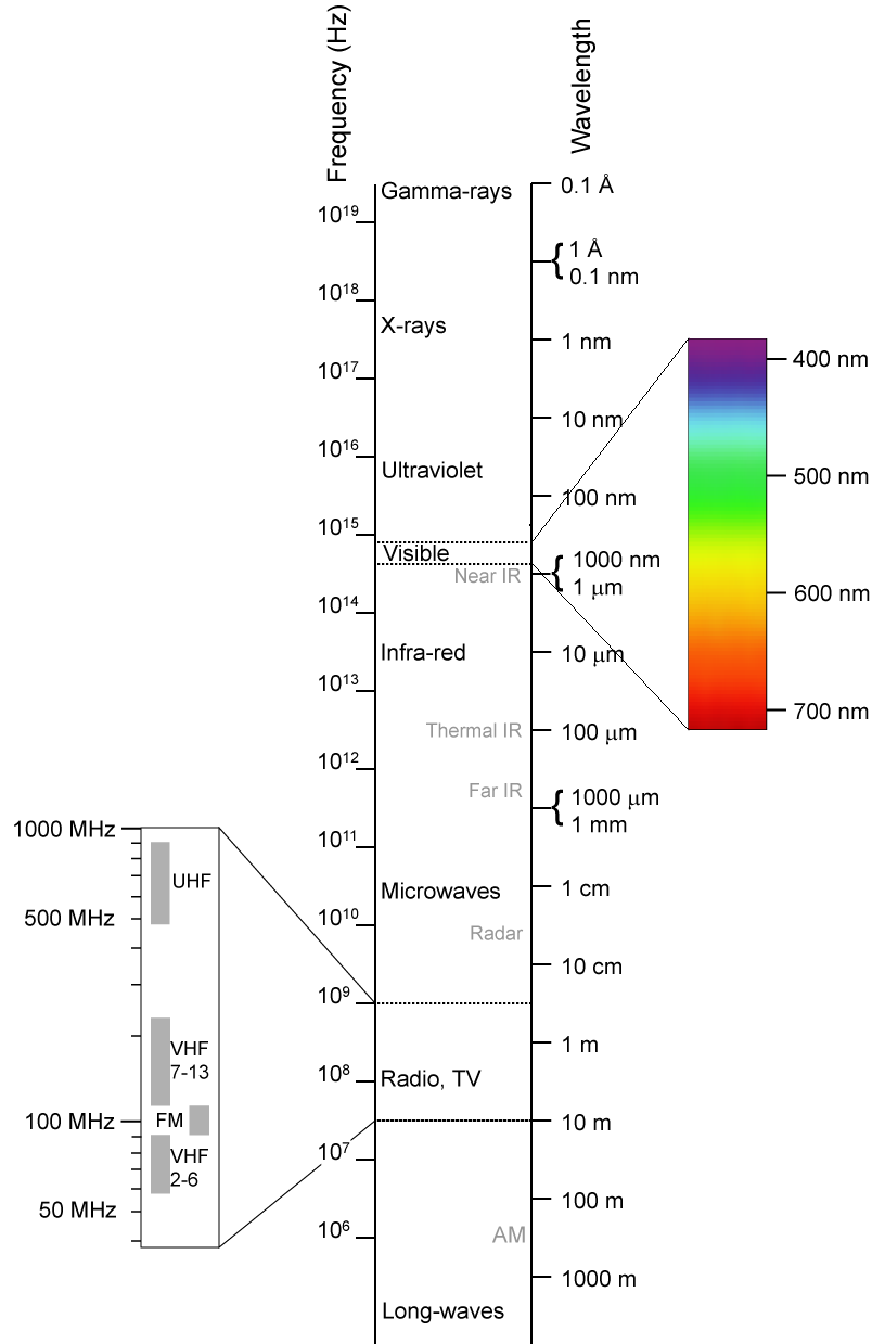
Author information
Authors and Affiliations
Corresponding authors
Editor information
Editors and Affiliations
Rights and permissions
Copyright information
© 2012 Springer-Verlag Berlin Heidelberg
About this chapter
Cite this chapter
Schiavon, N. et al. (2012). Applying the Techniques on Materials II. In: Varella, E. (eds) Conservation Science for the Cultural Heritage. Lecture Notes in Chemistry, vol 79. Springer, Berlin, Heidelberg. https://doi.org/10.1007/978-3-642-30985-4_6
Download citation
DOI: https://doi.org/10.1007/978-3-642-30985-4_6
Published:
Publisher Name: Springer, Berlin, Heidelberg
Print ISBN: 978-3-642-30984-7
Online ISBN: 978-3-642-30985-4
eBook Packages: Chemistry and Materials ScienceChemistry and Material Science (R0)