Abstract
Production of organic matter in the ocean is a fundamental process for biogeochemical cycling of elements (carbon, nitrogen, etc.) as well as for providing the foundation of nearly all marine food webs. Satellite remote sensing provides the only means of estimating this rate at basin and global scales. A variety of satellite-based models for estimation of net primary production exist spanning a wide range of complexity. Results from applying these models to the satellite record have yielded valuable insight on the ocean’s role in the earth climate system and the coupling of physics and biology. A vision for the next generation of NPP models aimed at utilizing existing tools and anticipated improvements in future satellite ocean color missions is also given.
Access provided by Autonomous University of Puebla. Download chapter PDF
Keywords
- Gross Primary Production
- Mixed Layer Depth
- Ocean Color
- Assimilation Efficiency
- Photosynthetically Available Radiation
These keywords were added by machine and not by the authors. This process is experimental and the keywords may be updated as the learning algorithm improves.
8.1 Introduction
Nearly one third of annual anthropogenic CO2 introduced to the atmosphere each year ends up in the ocean, with much of it mediated by biological uptake initiated by photosynthetic conversion of CO2 to organic matter. Quantification of marine photosynthesis has been the subject of study since prior to the twentieth century (see review by Barber and Hilting 2002 on the history of plankton productivity studies in the ocean). Photosynthetic primary production in the ocean relies on a diverse community of planktonic algae (phytoplankton) distributed across a wide range of oceanic habitats. The standing stock of phytoplankton at any time is small (≤1 Pg C), yet amazingly their cumulative rates of annual net primary production (NPP) equal or even exceed those of terrestrial plants (Field et al. 1998; Behrenfeld et al. 2001). NPP is defined as the fraction of total photosynthetic carbon fixation available for phytoplankton growth or consumption by the heterotrophic community and is a rate (generally expressed in units of carbon production per unit time). Variability in basin-scale marine NPP is clearly associated with climate fluctuations that are expressed as interannual changes in the environment, periodic phenomena such as El Niño/La Niña cycles, and glacial-interglacial transitions. However, ocean NPP is not simply forced by climate, but also participates in complex feedbacks governing climate (e.g., Falkowski et al. 1998a). Understanding the distribution of NPP and its environmental dependencies is thus critical for evaluating ocean biogeochemical cycles and climate change. In addition, NPP is the foundation of nearly all marine food webs. Organic matter produced through photosynthesis supports grazing by zooplankton and other herbivorous organisms and ultimately all carnivorous invertebrates and vertebrate fish and mammals. Although quantitative links between NPP and higher trophic levels have been difficult to establish (Friedland et al. 2012), NPP is a critical input variable for many types of fisheries models and is used as a constraint when evaluating harvestable catches (Sherman et al. 2009; Chassot et al. 2010; Pauly and Christensen 1995).
Assessment of NPP rates has relied primarily on traditional shipboard sampling which is costly, laborious, and provides coarse spatial and temporal resolution. The only viable approach for basin or global scale assessments has been through the use of airborne or satellite platforms. Radiometric measurements from early aircraft efforts provided the seed for remotely detecting phytoplankton, with an initial focus on assessing pigment (chlorophyll) concentration (Clarke et al. 1970). A first-order correlation exists between chlorophyll concentration and NPP, implying that successful remote sensing retrieval of the former property could yield estimates of the latter rate. In 1978, the Coastal Zone Color Scanner (CZCS) was launched and represented the first dedicated satellite ocean color sensor for estimating pigment concentrations, and subsequently NPP (Gordon et al. 1980; Hovis et al. 1980). The CZCS effort was very successful and its data are still used in contemporary investigations for multi-decadal studies of ocean color (e.g., Martinez et al. 2009; Antoine et al. 2005). Linking a fundamental radiometric quantity (satellite radiance) to a high-level rate process (NPP) has remained a key justification for modern ocean color satellite missions (e.g., SeaWiFS, MODIS). Pre-launch documents for these missions have explicitly identified NPP as a Level 4 product calculable from a combination of lower level products (Falkowski et al. 1998b; Esaias 1996). Even today, NPP remains a key ocean biological rate process targeted by all active satellite ocean color missions.
Accurate assessment of global ocean NPP is a daunting task. Much of the phytoplankton community contributing to production lies ‘hidden’ below the shallow surface layer detected by satellite sensors. The conversion of detected standing stocks to a rate processes remains a major challenge and is complicated by a variety of phytoplankton physiological attributes. Nevertheless, significant progress has been made since the launch of the CZCS with respect to evaluating ocean NPP and detecting its dependency on climate forcings. In this review, we begin with a general overview of the theoretical basis for remote sensing NPP algorithms, describe contemporary approaches, and discuss the validation of derived products. We then review some of the major findings regarding global ocean NPP and its variability and conclude with a discussion of new directions for improving our retrieval and understanding of this critical ecosystem property.
8.2 Theoretical Basis
Field measurements of ocean primary production were made throughout the twentieth century, but the modern measurement of NPP using radiolabeled carbon (14C) can be traced to Steeman-Nielsen (1952). Following its introduction, application of the 14C technique proliferated in oceanographic field studies, owing to its ease of use, high sensitivity, and ability to yield production estimates following a relatively short sample incubation period. Early 14C studies provided fundamental insights that were soon incorporated into NPP modeling efforts. Simple empirical relationships between NPP and Chl or ambient light (PAR) emerged as some of the first predictive expressions for aquatic NPP (Ryther and Yentsch 1957; Talling 1957; Vollenweider 1966). Subsequent modeling efforts have focused on a variety of additional factors, including detailed descriptions of the underwater light field (Morel 1991; Smyth et al. 2005), improved characterization of physiology (Armstrong 2006; Westberry et al. 2008), and definition of regionally-specific properties (Longhurst et al. 1995; Arrigo et al. 2008b). Unfortunately, the increasing complexity of NPP models has often not translated into improved predictive ability (see Sect. 8.4) and even the most complex satellite NPP models remain necessarily crude representations of the photosynthetic variability revealed by genetic, biochemical, and physiological laboratory studies.
While remote sensing retrieval of NPP is challenging, its fundamental relationship is straight forward. By definition, NPP in a given water parcel is the product of the extant phytoplankton biomass (expressed in the same currency as NPP, carbon) and its specific growth rate (μ),
The two quantities, Cphyto x μ, encapsulate dependencies on several aspects of the phytoplankton growth environment. For example, biomass (Cphyto) reflects a balance between growth and loss processes, such as grazing by zooplankton. By contrast, μ is largely a function of light and nutrient availability.
Equation 8.1 represents the fundamental relationship for NPP, but it is not the basis for most remote sensing NPP algorithms because both Cphtyo and μ are grossly undersampled in the ocean, largely due to methodological difficulties. In practice, chlorophyll concentration (Chl) has served as the central metric of phytoplankton standing stock. Conversion of Chl into NPP thus requires a characterization of assimilation efficiency (i.e., net primary production per unit chlorophyll; Pb). Much of the current error in NPP estimates results from unconstrained variability in this ‘photosynthetic efficiency’ term (Milutinovic and Bertino 2011; Behrenfeld and Falkowski 1997a). Pb is a function of incident photosynthetically available radiation (PAR) and thus varies with time of day, depth in the water column, season, and cloudiness. Fully resolved NPP models attempt to characterize this variability in the dynamic underwater light field. However, many simpler NPP algorithms employ time- and depth-integrated parameters and calculate productivity as a function of incident daily PAR and a maximum daily assimilation efficiency for the water column \( \left( {{\text{P}}_{\text{opt}}^{\text{b}} } \right) \). Behrenfeld and Falkowski (1997a) summarize and compare the various classes of models, distinguishing between approaches by time, depth, and wavelength resolution.
A key derived property for many ecological applications is daily water-column–integrated NPP (∑PP). In addition to subsurface light availability described above, assessment of ∑PP requires assumptions regarding other depth-dependent properties. In particular, surface mixed layer depth and vertically-varying nutrient loads, grazing pressures, and light conditions give rise to variations in biomass and phytoplankton physiological state (photoacclimation and growth rate). Numerous approaches have been developed to account for these effects. Depth-integrated models generally assume the water column is composed of two layers, one light saturated and the other light limited. An empirical function then relates the fraction of the water column that is light saturated to the incident irradiance. Behrenfeld and Falkowski (1997a) demonstrate that this approach is sufficient to capture >80 % of the variance in observed ∑PP when evaluated over a wide range of trophic conditions. Depth-resolved NPP models may take many forms. In some cases, vertical structure is prescribed using empirical relationships with surface properties (e.g., characterizing the profile of chlorophyll from surface chlorophyll concentration). More complex approaches incorporate information on mixing depths to assign an upper layer of uniform biomass and physiology, and then below this depth iteratively adjust chlorophyll stocks and physiological state based on models of photoacclimation, attenuation, and a prescribed shift from nutrient limitation to light limitation at depth (e.g., Westberry et al. 2008). As our knowledge of vertical variability improves, it will be these depth-resolved models that will provide the appropriate model scaffolding to incorporate this information to achieve improved NPP assessments.
All chlorophyll-based models of NPP, from simple depth-integrated algorithms to fully resolved time- and depth-dependent models, require a characterization of assimilation efficiencies (\( {\text{P}}^{\text{b}} ,\,{\text{P}}_{{^{\text{opt}} }}^{\text{b}} \), etc.). In most cases, this aspect of NPP models is least mature. The most common approach is to relate assimilation efficiency to sea surface temperature (SST), with a somewhat bewildering array of SST-dependent models proposed (see Fig. 8.4 in Behrenfeld and Falkowski 1997a). One of the most commonly employed functions expresses assimilation efficiency as an increasing exponential function of temperature. The Q10 for this exponent was based on a compilation of laboratory phytoplankton growth rates, where an exponential relationship was fit to the maximum observed growth rates over a wide range of temperatures (after Eppley 1972). There is no a priori reason to assume that this growth-rate-based function has any direct physiological relevance to the calculation of mean assimilation efficiencies. Behrenfeld and Falkowski (1997b) introduced an alternative temperature-dependent function that has also been widely applied. In their relationship, assimilation efficiency increases approximately exponentially up to 20 °C and then decreases, with a Q10 for the lower temperature range being similar to that of the ‘Eppley curve’. The Behrenfeld and Falkowski relationship was empirically derived from field 14C data and the down-turn in efficiencies at >20 °C was interpreted to reflect effects of nutrient stress. It is now recognized that nutrient stress, in and of itself, is not synonymous with a reduction in photosynthetic efficiency (Halsey et al. 2010; Parkhill et al. 2001). Thus, there is also no clear physiological basis for the temperature-dependent function of Behrenfeld and Falkowski (1997b).
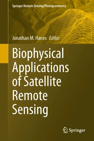
Development of new approaches for characterizing spatial-temporal variability in phytoplankton assimilation efficiencies is essential to advancing global ocean NPP estimates if surface chlorophyll concentration continues to be the remotely detected property of choice for phytoplankton biomass. Clearly, these advances must be based on a fundamental understanding of physiological responses to environmental growth conditions, rather than empirical relationships with SST. Nevertheless, employment of simple SST functions has yielded NPP estimates that exhibit reasonable relationships with field measured values. So, what is the basis of this success? The most likely explanation is that SST can, at times, function as a surrogate for an environmental factor directly governing variability in assimilation efficiency: light. Phytoplankton acclimate to changes in light conditions on time scales of days to a week or more. A decrease in incident light or an increase in mixing depth results in an increase in cellular chlorophyll. This light-driven increase in chlorophyll is not paralleled by an increase in carbon fixing capacity and thus results in a lower apparent assimilation efficiency (i.e., NPP/Chl decreases). In nature, regions of low incident light and/or deep mixing also tend to have lower SST. Thus, lower SST is broadly associated with low growth irradiance (Ig) and, thus, lower assimilation efficiencies. This tendency is illustrated in Fig. 8.1a where mean mixed layer light levels (Ig) exhibit roughly an exponential positive relationship with SST when evaluated over the global open ocean. The increase in Ig with SST drives a physiological acclimation that yields increasing assimilation efficiency with increasing SST. As a result, the implied change in cellular chlorophyll content viewed as a function of SST exhibits a pattern remarkably similar to expected changes as a function of Ig (Fig. 8.1b).

Demonstration of covariance between mixed layer growth irradiance (Ig) and sea surface temperature (SST). a Panel on left shows classical relationship between SST and Pb opt (red line) derived from Eppley (1972). Also shown is the median Ig (blue line) within discrete SST bins, calculated following Westberry et al. (2008). b Panel on right shows an idealized photoacclimation response (Chl:C, red line), where the dependent variable, Ig, has been scaled to match the range of SST. Blue line shows the same Chl:C as a function of SST. In both cases, Chl:C is expressed relative to a high light value of 1 (units not important)
8.3 Methods
Satellite sensors provide a range of geophysical products relevant to NPP calculations, with three central properties being chlorophyll concentration, cloudiness-corrected PAR, and sea surface temperature (SST). These 3 variables are sufficient to initiate many NPP models (e.g., Behrenfeld and Falkowski 1997b), while other models require additional inputs. For example, some models require information on mixed layer depths (Howard and Yoder 1997; Westberry et al. 2008) or employ precalculated lookup tables (Antoine et al. 1996; others). Some recent NPP models have been developed that are based on inherent optical properties derived from ocean color inversion algorithms, including phytoplankton absorption coefficients (Lee et al. 1996) and/or particulate backscattering coefficients (b bp ) (Westberry et al. 2008). In many cases, NPP models can be viewed as modular in construct, in the sense that alternative formulations can be readily substituted. For example, the Vertically Generalized Production Model (VGPM) of Behrenfeld and Falkowski (1997b) is often executed with different temperature functions for \( {\text{P}}_{\text{opt}}^{\text{b}} \), most often with exponential Eppley-type dependence.
While most global-scale NPP algorithms are based on chlorophyll as the index of standing stock, a notable exception is the model of Westberry et al. (2008). In their approach, phytoplankton carbon concentration is inferred from satellite b bp data and used as the core biomass index. Simultaneous satellite retrievals of chlorophyll and carbon concentrations are then used to directly infer information on physiological status of phytoplankton within the surface mixed layer using understanding of Chl:C variability from laboratory studies. The Westberry et al. model is both depth and wavelength resolved, but is also unique in that it operates iteratively through the water column. Specifically, the model assumes biomass and physiological uniformity within the mixed layer, and then iteratively calculates spectral irradiance at each subsequent depth horizon as a function of integrated changes in biomass, pigment, and attenuation directly above. The resulting light field, in turn, defines the photoacclimation state (i.e., cellular pigmentation) of the phytoplankton within the current depth horizon and their growth rate. Finally, in regions of surface macronutrient depletion, the model allows for a switch from nutrient-limitation to light-limitation at depths below the mixed layer. While additional work is needed to validate various aspects of this ‘carbon-based approach’, it does provide an excellent framework for incorporating more sophisticated descriptions of physiological variability (see Sect. 8.6).
8.4 Validation Efforts
Validation of satellite-based NPP estimates has largely been limited to matchup comparisons with field 14C uptake measurements. While considerable ambiguity remains regarding exactly what the 14C method measures, it is generally accepted that reasonably long (i.e., >12 h) incubations yield carbon fixation rates that approximate net primary production. The ‘ambiguity’ of the measurement includes unconstrained artifacts of sample confinement in bottles, unnatural light conditions during incubation (either on deck of the ship or in situ), and an incomplete understanding of how respiratory and other metabolic pathways impact lifetimes of newly formed carbon products. Alternative measures of photosynthetic primary production (e.g., gross primary production) are less frequently used for validation of satellite-based estimates. Both, 18O2 incubations and the more recently developed triple-oxygen isotope method (17∆O2) provide a measure of gross primary production. Importantly, the latter method does not require sample incubations (Luz and Barkan 2009). However, empirical conversions are required to equate the different oxygen and carbon measurements and to characterize losses between gross and net photosynthetic production. Hence, we limit the following discussion to comparisons with measurements of 14C uptake.
A series of blind, round-robin exercises were initiated by NASA in the mid-1990’s in order to evaluate the performance of a wide variety of satellite NPP models. This Primary Productivity Algorithm Round Robin (PPARR) exercise has since evolved in its scope and expanded in the range of model types, numbers, and field measurements represented (Campbell et al. 2002; Carr et al. 2006; Friedrichs et al. 2009; Saba et al. 2010, 2011). Key findings of the PPARR activities have been: (1) increasing model complexity does not equate to improved predictive skill, (2) model skill varies regionally, and (3) reducing uncertainty in input parameters to NPP models (e.g., PAR, Chl) can reduce average RMS errors by >50 %. The first point above has been made on several occasions (Siegel et al. 2001; Behrenfeld and Falkowski 1997a), but is perhaps best demonstrated by Carr et al. (2006). In their report, a cluster analysis was performed on the correlation between NPP estimates for >30 models, spanning a wide range of complexity. The analysis revealed that correlations between model NPP estimates were not grouped according to model complexity, such that the simplest and most complex models often showed the highest correlation. Instead, correlations between models were largely determined by the underlying expression used to describe variability in assimilation efficiencies (e.g., models that used an ‘Eppley-type’ formulation clustered together). The most comprehensive study demonstrating the second point was made by Saba et al. (2011). Output from 21 satellite-based ocean color models were analyzed against >1000 in situ 14C measurements from diverse ocean regions spanning the Black Sea, Southern Ocean, high latitude North Atlantic, and subtropical Pacific and Atlantic. Some of the results are reproduced in Fig. 8.2 which show the ensemble average root mean square error (RMSE) in each region. Lower RMSE results from better predictive ability of NPP models (no distinction between models is made here).

Average root mean square difference (RMSD) of 21 satellite NPP models evaluated against field 14C measurements for several different locations. Error bars represent 2x standard error. Blue portions of each bar represent maximum potential reduction in RMSD if uncertainties in model input and field measurements are accounted for. For details regarding specific models and field dataset used, see Saba et al. (2011)
The last finding listed above from the PPARR exercises underscores that a model’s ability to accurately predict NPP is highly dependent upon the uncertainties inherent in the input data (Fig. 8.2) (Saba et al. 2011). While this may seem obvious, it is often difficult to propagate errors through complex analytical formulations resulting in model NPP estimates being reported with no accompanying error estimates. Saba et al. (2010) found that the majority of models were unable to accurately reproduce the observed trends in NPP at open ocean sites in the North Pacific (Station ALOHA near Hawaii) and the Atlantic (BATS near Bermuda). However, holding all other properties the same, but employing in situ estimates of Chl in the NPP models allowed many of the models to match the sign, and to a lesser extent, the magnitude of the observed trends in NPP. Siegel et al. (2001) also demonstrated the influence of using time-varying or site-averaged photosynthetic parameters in NPP models at BATS and found the predictive ability dropped significantly (r2 = 0.80 to r2 = 0.27) when mean values were used.
8.5 Major Findings
One of the fundamental realizations provided by remote sensing estimates of marine NPP is that the ocean contribution to biospheric annual NPP is roughly equivalent to that from terrestrial sources. Field et al. (1998) first synthesized global estimates of marine NPP from the VGPM and terrestrial NPP from the CASA model (Potter et al. 1993). Although state-of-the-art at the time, the averaging periods for land and oceans were significantly different, the spatial resolutions were coarse, and quality for the ocean color data was well below today’s standards. Nevertheless, the global picture that emerged indicated a marine NPP contribution of ~49 Pg C of the combined 105 Pg C for the biosphere. Compilation of historical estimates of oceanic NPP based on 14C measurements yields a mean value similar to the Field et al. (1998) satellite-based estimate, but uncertainty in the field-based assessment is large enough to render the estimate meaningless (see Barber and Hilting 2002 for a chronology of global NPP estimates).
Recalculation of biospheric NPP using more recent data than employed by Field et al. (1998) yields values for a typical year (2004) of 54 and 50 Pg C year−1 for the oceans and land, respectively. Figure 8.3 shows the spatial distribution of combined land and ocean NPP, where both estimates are based on MODIS remote sensing data (Zhao et al. 2005; Behrenfeld and Falkowski 1997b). While maximum values of areal NPP rates can be substantially higher on land than in the ocean, the much greater spatial extent of ocean area mitigates this difference in zonally integrated values (Fig. 8.3). From the zonal profiles we find that tropical NPP on land is approximately twice that of equatorial marine primary production. Northern boreal forests (between 40°N and 60°N) are also a factor of 2× higher than oceanic totals across the same latitude domain. Marine NPP dominates southern hemisphere NPP south of 25°S.

a Average annual satellite NPP (gC m-2 yr-1) from a combination of terrestrial and oceanic sources. b Right-hand panel shows zonally integrated NPP (Pg C yr-1) for land (green line) and ocean (blue line) areas
Many of the major findings which remote sensing of NPP has enabled are related to improving our understanding of the links between physical forcing (e.g., climate) and biological response in the ocean. For example, the El Niño-Southern Oscillation (ENSO) phenomenon is a periodic climate perturbation that elicits significant changes in a wide array of marine ecosystem properties. The first modern era ocean color satellite (SeaWiFS) was launched during one of the largest ENSO events on record. The first 3 years of the mission captured the peak of the El Niño event and the following transition to an equally large La Niña (Behrenfeld et al. 2001). The peak to peak change in ocean NPP across this transition (~6 Pg C) exceeds any other anomaly since observed in the satellite ocean color record (Arndt et al. 2010; Blunden et al. 2011). El Niño is accompanied by higher than normal SST throughout much of the tropical Pacific Ocean and interrupts the normal upwelling pattern which supports significantly elevated NPP in the eastern tropical Pacific. Field studies have estimated reductions in nutrient supply and NPP of ~80 % during El Niño (Barber and Chavez 1983; Chavez et al. 2002). A similar relationship was reported by Behrenfeld et al. (2006a) over the entire stratified surface ocean (~40°N to 40°S) based on remote sensing estimates of NPP.
A central objective underlying the development of a long-term, climate-quality satellite ocean color data record is to improve understanding of climate-ocean ecology interactions. It has been estimated that 50 or more years of continuous satellite observations will be necessary in many ocean regions to clearly detect the signature of anthropogenic impacts from natural variability (Henson et al. 2009). Clearly, this is far too long to wait. However, over much shorter time scales, natural forms of climate variation can provide critical insights on NPP and phytoplankton biomass variability. To this end, Behrenfeld et al. (2006a) showed that over the first 10 years of SeaWiFS observations, anomalies in water column integrated chlorophyll and modeled NPP (VGPM and CbPM) integrated over the permanently stratified oceans (i.e., annual average SST >15 °C) were highly correlated with variations in SST and surface mixing depths. Furthermore, the spatial distribution of NPP anomalies mirrored those of SST anomalies.
The Behrenfeld et al. (2006a) study has been followed by a series of similar analyses. In Behrenfeld et al. (2008), the strong correlation between chlorophyll and SST anomalies was also shown to occur at higher northern latitudes, but no significant trends were found for the Southern Ocean. This latter conclusion was repeated by Arrigo et al. (2008b) who reported no significant trend in Southern Ocean NPP between 1998 and 2006. Annual totals for the domain south of 50°S were ~2 ± 0.07 Pg C year−1, nearly half of previous remote sensing based estimates for this region. Martinez et al. (2009) significantly expanded the time period of evaluation by combining SeaWiFS data with the earlier CZCS record. Their study again reported significant inverse relationships between global ocean SST and chlorophyll anomalies, both in regionally integrated data and spatially-resolved fields. With this expanded data set, these authors were also able to clearly identify impacts of the longer time-scale climate fluctuations associated with ocean basin decadal oscillations. Additional analyses of temporal ocean color data employing both SeaWiFS and MODIS measurements were provided in reports by (Arndt et al. 2010; Blunden et al. 2011). Interestingly, several recent studies addressing temporal changes using in situ measured NPP have reported conflicting results from those found using satellite data (Dave and Lozier 2010; Lozier et al. 2011; Saba et al. 2010; Chavez et al. 2011). These differences highlight the difficulty in comparing quantities and trends derived from singular locations representing small spatial scales to integrated signals over entire ocean basins.
An important question arising from the aforementioned studies was what the underlying basis is for the inverse relationship between chlorophyll and SST anomalies. The magnitude of the SST anomalies is far too small to be directly responsible for the observed chlorophyll responses. Instead, and as suggested by Behrenfeld et al. (2006a), changes in SST are likely functioning as a proxy for altered surface mixing depths, where shallower mixing is accompanied by decreasing chlorophyll. Two mechanisms likely contribute to the link between surface chlorophyll concentrations to mixing depth: an impact on vertical nutrient transport from depth and changes in the average light level experienced by surface phytoplankton. To distinguish which of these two factors dominate, Behrenfeld et al. (2008) separated chlorophyll variability in permanently stratified ocean into that due to biomass changes and that due to intracellular chlorophyll (Chl:carbon) changes. Their study showed that, over most of the SeaWiFS record, chlorophyll variability was largely due to physiological changes in Chl:carbon and that most of this variability was attributable to changes in the upper ocean light environment, not nutrients. These findings imply that significant variations in chlorophyll detected in the satellite record are likely not linked to parallel changes in NPP. However, most contemporary NPP models are not equipped to make this distinction (see Sect. 8.6.1). More recently, Siegel et al. (2013) extended the analysis of physiological variability to all global ocean regions and additionally showed that apparent anomalies in chlorophyll may be, in part, traceable instead to variations in colored dissolved organic material. Taken together, these studies once again emphasize that careful attention must be given to physiological attributes if global ocean NPP and its temporal variability are to be accurate evaluated.
As global, synoptic estimates of NPP have advanced, opportunities have arisen for investigating relationships between NPP and more derived, yet critical, carbon cycle parameters. For example, the fraction of NPP delivered from the surface ocean to depth is a critical quantity of interest when addressing the ocean’s role in carbon sequestration. This export production is traditionally measured in the field using sediment traps that collect and preserve sinking material, but these measurements have longstanding caveats (Buesseler et al. 2007 and references therein) and are extremely sparse in both space and time. Satellite observations of NPP, when combined with ecosystem model results and field measurements have provided simple, yet powerful empirical parameterizations that allow globally resolved fields of export production (Laws et al. 2000; Dunne et al. 2005). Current estimates of export production are ~10 Pg C year−1 globally and its spatial distribution gives us insight into ecosystem functioning. For example, Laws et al. (2000) showed that the Atlantic and Pacific Oceans contribute equally to total export (~4.3 Pg year−1 each), despite their two-fold differences in size (~75 × 106 km2 and ~160 × 106 km2, respectively). Recently, Westberry et al. (2012) applied satellite NPP estimates to field-derived photosynthesis-respiration relationships to characterize global ocean respiration rates and net community production. These net community production rates set an upper constraint on export production for comparison with alternative approaches. Validation of these advanced, satellite-based carbon cycle parameters has yet to be carried out and should be an active research area in the future (see following section).
8.6 Future Research Directions
As detailed herein, significant progress has been made in quantifying NPP from global satellite data and applying these estimates to ecological questions, yet opportunities abound for making major improvements. Such improvements may take a variety of forms, including greater accuracy of NPP retrievals when compared to field measurements, development of new field metrics for validation, exploitation of advances in future satellite design capabilities, and more sophisticated physiological formulations in NPP models. Some of these improvements are relatively straightforward and may entail advances in engineering (e.g., higher spectral/spatial resolution on future ocean color sensors), while others will be more challenging (treatment of phytoplankton physiology). In this final section, we attempt a forward-looking view at potential avenues for refining global NPP assessments, particularly with respect to advancing characterization of physiological attributes.
8.6.1 Photoacclimation
Global surface ocean chlorophyll concentrations vary by roughly 3 orders of magnitude. Physiological changes in intracellular chlorophyll from varying light and nutrient conditions can span over 1.5 orders of magnitude, with the light effect alone (i.e., photoacclimation) contributing up to a factor of 10 variability (Falkowski and Laroche 1991). While variability in chlorophyll concentration due to changes in biomass or nutrient availability is positively correlated with changes in NPP, changes in chlorophyll due to photoacclimation are inversely correlated with NPP. In other words, all else being constant, an increase in daily light exposure results in a decrease in chlorophyll and an increase in assimilation efficiency. Given the magnitude of the photoacclimation response, it is somewhat surprising therefore that this physiological property is routinely ignored in all but a few marine NPP models. Even an imperfect assessment of photoacclimation could significantly improve NPP predictions and does not require a highly sophisticated model to effectuate. For example, the simple wavelength- and depth-integrated VGPM could be applied to satellite chlorophyll fields that are first corrected for photoacclimation. For this approach, global data on incident PAR, diffuse attenuation (Kd), and mixed layer depths (MLD) are needed to calculate Ig. Next, a laboratory-based relationship between Ig and cellular chlorophyll content can be employed to normalize satellite chlorophyll data to a uniform photoacclimation state and then these data applied in the VGPM with a constant value for \( {\text{P}}_{\text{opt}}^{\text{b}} \). In essence, this strategy is equivalent to the approach of the Carbon-based Production Model (CbPM) of Westberry et al. (2008). The CbPM distinguishes Chl variability into that due to biomass changes and intracellular pigmentation. The latter property is then divided into light- and nutrient-dependent terms, where the photoacclimation effect is determined from PAR, Kd, and MLD. The residual Chl:C variability is due to nutrient effects and is linearly proportional to NPP variability.
An important aspect of characterizing photoacclimation in the mixed layer (i.e., the portion of the water column sampled from space) is identifying the light level to which a natural phytoplankton community is acclimated. The uppermost reaches of the surface ocean are a turbulent, well mixed environment where a given phytoplankton population may circulate through a typical mixed layer of 50 m thickness >10 times per day (D’Asaro 2003). Laboratory studies indicate that the light-dependent signal for chlorophyll synthesis is keyed to the redox state of the plastoquinone (PQ) pool between photosystem II and photosystem I (Escoubas et al. 1995). An oxidized PQ pool signals for chlorophyll synthesis, while a reduced pool indicates that adequate chlorophyll (i.e., light harvesting capacity) exists. PQ pool reduction occurs at all saturating light levels, thus regulation of pigment synthesis is essentially an on–off switch (i.e., once light exceeds saturation, the signal for chlorophyll synthesis is off and further increases have no additional impact). Acclimation in such a system is thus best characterized as a function of the median light level within the mixed layer, rather than the average light level with is impacted by light levels in excess of saturation. The remaining issue is spatially- and temporally characterizing global MLD. Unfortunately, MLD is not a property directly retrieved by remote sensing. Consequently, we currently must rely on model or model-data assimilation schemes to generate the necessary MLD fields (e.g., Clancy and Sadler 1992). Notably, significant uncertainty remains in these MLD products, particularly at high latitudes (e.g., Southern Ocean), reducing this uncertainty will make a significant contribution toward advancing NPP assessments.
An additional issue regarding characterization of phytoplankton photoacclimation is distinction between the ‘physiological’ mixed layer depth from ‘physical’ mixed layer depth calculated from water column density or temperature properties. For much of the year and many parts of the ocean, there may be little difference between the ‘physiological’ and ‘physical’ mixed layers, but under certain, important conditions significant differences may exist. For example, the onset of winter-spring stratification in temperate and high-latitude seas can be rapid and non-monotonic. During this period, photoacclimation of the phytoplankton community will be responding to changes in the mixed layer light environment on timescales of order ~1–2 weeks. Photoacclimation timescales are also dependent on the direction the light changes, taking longer when Ig is decreasing than when it is increasing. At timescales significantly <1 week, it is likely that passage of brief mixing events (associated with meteorological fronts) will not be registered by the phytoplankton, whereas the physical mixed layer depth may be significantly perturbed for a day or so, then return to its previous position. A practical approach to estimate a physiological MLD may exist through the use of dissolved O2 profiles. Castro-Morales and Kaiser (2012) demonstrated the utility of this approach over a limited geographic region and found significant differences from traditional hydrographically determined mixed layers.
8.6.2 Nutrient Effects
Short-term perturbations in macronutrient availability can result in a brief period of unbalanced growth where phytoplankton assimilation efficiencies are reduced. However, under the steady state conditions found across most of the ocean, phytoplankton are well acclimated to their nutrient environment. Under such conditions, cellular chlorophyll levels are adjusted in direct proportion to nutrient availability and apparent assimilation efficiencies can be as high as under nutrient replete growth. Thus, the long-held assumption that nutrient stress is associated with inefficient photosynthesis is largely incorrect. This conclusion is supported by laboratory work demonstrating highly tuned photosynthetic light harvesting capacities optimized to macronutrient-defined growth rates (Laws and Bannister 1980).
While the aforementioned considerations suggest that assessing nutrient status may not be as critical once thought for assessing global ocean NPP, this conclusion may not be valid for conditions of iron stress. Iron concentrations are vanishingly low over much of the open ocean, and phytoplankton have evolved a variety of strategies for optimizing iron economy (Behrenfeld and Milligan 2013). These adjustments, however, can have a significant impact on apparent assimilation efficiencies, particularly under conditions where macronutrients are replete. Greater than one-third of the ocean surface area has conditions of low iron and high macronutrients (the so-called High-Nutrient, Low-Chlorophyll (HNLC) regions). Ironically, recent studies have shown that phytoplankton under HNLC conditions actually over-express chlorophyll synthesis relative to growth (Behrenfeld and Milligan 2013; Schrader et al. 2011; Behrenfeld et al. 2006b). This excess Chl does not contribute to photosynthesis (it is functionally “decoupled” from the photosystems), but is registered in satellite Chl retrievals. The pool of ‘dysfunctional’ Chl may account for >40 % of the total Chl in HNLC waters (Behrenfeld et al. 2006b; Schrader et al. 2011) and must be accounted for when assessing assimilation efficiencies. Behrenfeld et al. (2006b) estimated the magnitude of error in satellite NPP introduced by this bias in Chl over the Equatorial Pacific Ocean. The authors exploited field measurements of fluorescence signatures linked to functional and dysfunctional Chl and concluded that annual NPP for the region (using the VGPM and CbPM) may need to be revised downward by ~15 %.
Recent advances in our understanding of solar-stimulated chlorophyll fluorescence measured from satellite (i.e., MODIS, MERIS) may provide an avenue for correcting satellite Chl and NPP fields for Fe-stress effects globally. Similar to the field diagnostics of Fe-stress employed by Behrenfeld et al. (2006b), satellite Chl fluorescence registers the imprint of Fe-stress (Behrenfeld et al. 2009; Westberry et al. 2013). Due to the pool of dysfunctional Chl described above and to shifts in photosystem stoichiometry occurring under iron stress (Behrenfeld and Milligan 2013), higher intrinsic fluorescence yields are observed in iron-stressed ocean region under the high light conditions of satellite fluorescence measurements. As a demonstration of this link between Fe-stress and satellite Chl fluorescence, Westberry et al. (2013) showed that purposeful addition of Fe to natural phytoplankton communities resulted in a marked decrease in satellite-based chlorophyll fluorescence efficiency. Further evidence was given by Behrenfeld et al. (2009) who highlighted the tight correspondence between regions of elevated MODIS fluorescence quantum yields and modeled regions of Fe-limitation and low dust deposition (the primary mechanism for Fe input to the open ocean). These findings imply that satellite-detected regions of elevated Chl fluorescence yields may provide an avenue for time-resolved assessments of phytoplankton assimilation efficiencies that can account for the unique physiological consequences iron stress. Furthermore, such an approach could account for the highly dynamic nature of iron supply, which can be linked to episodic upwelling or atmospheric deposition events.
8.6.3 Phytoplankton Community Composition
It has long been recognized that ocean NPP exhibits strong regional variability and that some of this variability is tied to community taxonomic structure. Regionally specific NPP algorithms have been employed to indirectly account for taxonomic variability. For example, several studies have partitioned the ocean into distinct ‘biogeographical provinces’ that are empirically assigned unique photosynthetic parameters (Longhurst et al. 1995; Sathyendranath et al. 1995). This approach draws upon extensive field data sets of 14C uptake data and avoids any necessity for explicit predictive relationships. Alternatively, empirical predictive relationships may be derived for specific broad ocean regions, such as the Arctic or Southern Ocean (Arrigo et al. 2008a, b).
In addition to influencing regional variability, taxonomic contributions to NPP have relevance to understanding ecosystem carbon flow, export efficiency, and fisheries production (Ryther 1969), for example. A variety of satellite ocean-color based studies have aimed to directly decompose bulk emergent bio-optical signals into contributions from different phytoplankton groups. While few models have been successful at resolving species-level differences in satellite ocean color data (Westberry and Siegel 2006; Balch et al. 2005; Alvain et al. 2008; Bracher et al. 2009), algorithms do exist for identifying broad phytoplankton size classes (Ciotti et al. 2002; Devred et al. 2006; Uitz et al. 2006; Hirata et al. 2008). These techniques rely on the first order relationship between cell size and ecosystem function (after Sieburth et al. 1978). However, the end-point of most of these studies has been to assess different phytoplankton size-class contributions to pigment biomass (Chl) only, rather than their contributions to NPP. For example, Uitz et al. (2006) used a large in situ dataset of Chl and other diagnostic pigment markers to generate empirical parameterizations between surface [satellite] Chl and relative dominance of three size classes of phytoplankton; pico-, nano-, and micro-phytoplankton. The link between size-fractionated Chl estimates and NPP was made in subsequent work by Uitz and co-workers who associated class-specific photophysiological variables with pigment-based size classes in field datasets (Uitz et al. 2008), then applied these relationships to satellite data (Uitz et al. 2010).
The approaches described above all suffer from their reliance on satellite Chl as an indicator of biomass. As a result, they interpret higher Chl as more biomass, and by inference, a greater contribution from larger size classes of phytoplankton. One solution to this problem in the context of remote sensing is to build on the body of work which employs satellite estimates of particulate backscattering (bbp) to quantify phytoplankton carbon directly (Behrenfeld et al. 2005; Westberry et al. 2008; Kostadinov et al. 2009). The global relationship of Westberry et al. (2008) relating particulate backscattering to Cphyto can be improved through (1) routine field measurements of Cphyto (currently there are none) to better constrain the relationship, (2) improvements in bio-optical inversion schemes that estimate bbp from satellite radiance, and (3) algorithm development that accounts for anomalous sources of bbp biasing estimates of Cphyto (e.g., coccolithophores). Kostadinov et al. (2009, 2010) recently introduced a remote sensing method for characterizing particle size distributions (PSD) based on spectral bbp retrievals. Resultant PSDs can be expressed as a continuous function of size and related to specific phytoplankton size ranges, such as pico-, nano-, and micro-phytoplankton. Given biovolume-specific carbon concentrations, which are available from laboratory studies, this method could yield class-specific carbon biomass explicitly. Perhaps an even more compelling avenue would be to combine the approaches of Uitz et al. (2006) and Kostadinov et al. (2009) to partition both Chl and Cphyto individually to characterize size-class specific Chl:Cphyto ratios. Any existing NPP model that accounts for Chl:Cphyto variability would surely benefit from this added information.
Another means of incorporating taxonomic information is through the use of phytoplankton absorption, aph, rather than Chl concentration. NPP models employing Chl implicitly assume a fixed Chl-specific absorption capacity, \( {\text{a}}_{\text{ph}}^{*} \), despite order of magnitude variability that exists in \( {\text{a}}_{\text{ph}}^{*} \) (Bricaud et al. 1995, 1998). Much of this variability can be related to the size distribution of extant phytoplankton and presumably taxonomic composition (Bricaud et al. 2004). Lee et al. (1996) provide a NPP model amenable to remote sensing which is cast in terms of aph, rather than Chl. For the dataset these authors investigated, aph-based NPP models were far superior to Chl-based analogs. In addition to the conceptual advantages of using aph over Chl for estimating NPP, retrieval of aph from satellite reflectance has also been suggested to be preferable to direct estimation of biogeochemical quantities such as Chl (Lee et al. 2002).
8.6.4 New Tools
The various avenues discussed above for improving global assessments of ocean NPP are largely focused on advances that can be made with currently available observational and model-derived data sets. Major future advancements, however, may also be realized through engineering developments, both in the ocean and in space. Autonomously collected data by free-drifting and profiling floats and gliders is already returning unprecedented measurements of physical, optical, nutrient, and oxygen properties. Already, these data have been used to track the seasonal evolution of phytoplankton blooms (Boss and Behrenfeld 2010) and constrain the upwelling supply of nutrients available for photosynthesis (Johnson et al. 2010), to name just a few applications. Following the success of the Argo program (Roemmich and Owens 2000), the Bio-Argo program strongly supports development and deployment of floats equipped with sensors for measuring key biogeochemical properties, such as Chl fluorescence and particulate backscattering. Similar efforts are in place to make routine O2 measurements on profiling float platforms (Gruber et al. 2007). Inclusion of these capabilities represents the first precursors to NPP-enabled floats. Indeed, prototype floats capable of the aforementioned measurements and more (e.g., radiometers) already exist and should enable a single platform to yield a complete suite of data suitable for initial NPP calculations.
Another exciting yet unexploited tool for ocean ecological studies is space-based lidar (Light Dectection And Ranging) systems. Lidar technology is widely used in terrestrial and atmospheric disciplines, but ocean applications have been limited to targeted near-shore and coastal studies using aircraft or ship-based systems (e.g., Churnside and Wilson 2001). Nevertheless, space-borne LIDAR assets are available for investigating their application to subsurface ocean retrievals. For example, the CALIOP lidar on the CALIPSO satellite conducts routine vertical profiling measurements at 532 and 1064 nm. The latter wavelength is too long to penetrate the ocean surface, but the former should effectively sample near surface plankton populations. CALIPSO’s stated science objectives are aimed atmospheric aerosol and cloud science applications. Nevertheless, preliminary analyses suggest subsurface scattering signals can be detected from the ocean surface. CALIOP was not designed for ocean applications, but these early results suggest that a more capable ocean-penetrating space lidar could provide critical independent constraints on ocean particle pools and perhaps even assessments of vertical structure in plankton distributions with links to mixed layer depths.
Significant opportunities also exist for realizing major advances in ocean ecosystem characterization from upcoming passive ocean color sensors designed with capabilities far exceeding those of our heritage sensors. Technological developments since the conception of CZCS, SeaWiFS, and MODIS now enable major improvements in spatial, temporal, and spectral resolution, although not necessarily all within a single instrument. Increased spectral resolution and expansion into the near-ultraviolet wavebands (350–400 nm) will allow further discrimination of different phytoplankton groups and separation of phytoplankton from other optical constituents (sediments, detritus, dissolved organics). Improved atmospheric corrections may also be realized by flying an advanced ocean color sensor with a profiling lidar and multi-angle spectral polarimeter. A satellite constellation of this sort will not only improve atmospheric corrections for more accurate water leaving radiance retrievals, but would also provide simultaneous lidar subsurface retrievals described above and a capacity for discriminating organic and inorganic particles through the polarimeter measurements (Loisel et al. 2008).
8.6.5 Vision for Future Remote Sensing of NPP
The preceding subsections outlined various avenues for advancing space-based NPP models. Here, an example is given which employs some of these pieces and allows a glimpse of how the distribution of NPP and our understanding may differ when taken into consideration. This new approach is termed the Carbon, Absorption, and Fluorescence Euphotic-resolving (CAFE) NPP model. For this exercise, the VGPM is used as a prototypical satellite NPP model, and its annual average NPP rate is shown in Fig. 8.4. In contrast, the CAFE NPP model assimilates new satellite-derived information into its estimation of NPP rates. First, the model employs satellite-derived estimates of particulate backscattering that are used to estimate phytoplankton carbon biomass (C) directly. This parameter also allows estimation of Chl:C which provides physiological information (i.e., photoacclimation) and a link to the phytoplankton growth rate, μ (Laws and Bannister 1980). Thus, we can estimate NPP directly using Eq. 8.1. Using this approach, the model is able to distinguish physiological changes in cellular pigmentation from changes in biomass. The result is that many high Chl regions (i.e., North Atlantic) have reduced NPP as some fraction of the bulk Chl is attributed to photoacclimation. In contrast, many low Chl regions (i.e., North Pacific Subtropical Gyre) exhibit increased NPP relative to the VGPM as their biomass (and Chl) may be low, but their growth rates can still be high. Second, chlorophyll fluorescence from satellite has been shown to register the unique imprint of iron stress over much of the ocean (Behrenfeld et al. 2009; Westberry et al. 2013). The reason for this, in part, results from chlorophyll present in phytoplankton and reflected in satellite-based Chl retrievals, but which is dissociated from photosynthetic electron transport (Behrenfeld and Milligan 2013). Therefore, NPP models which employ Chl as a biomass indicator will tend to overestimate NPP where phytoplankton are iron stressed. Satellite estimates of chlorophyll fluorescence efficiency (φf, Behrenfeld et al. 2009) can be used to correct for this effect (Fig. 8.4). Here, a simple linear correction is applied that assumes the strength of iron limitation is directly proportional to φf above some threshold value that marks the onset of iron limitation. The effects are largely irrelevant outside the equatorial oceans, but can reduce NPP by up to 40 % in some places. This is consistent with the observation that up to 40 % of the total Chl content in iron stressed cells can be in a ‘dissociated’ state (Moseley et al. 2002). In the example given, this correction alone decreases global annual, marine NPP by >3 Pg year−1, nearly all of which is in the tropics between 20°N and 20°S. Third, the CbPM can be recast in terms of phytoplankton absorption (aph) per unit carbon rather than Chl:C. This approach has the benefit of accounting for all accessory pigments which can play an important role in light absorption and photosynthesis. Absorption-based NPP modeling has shown superior predictive ability in some field datasets (Lee et al. 1996). In addition, this approach should also reduce uncertainties arising from empirical retrievals of Chl, as phytoplankton absorption is more closely tied to the fundamental satellite measurements of radiance.

Illustration of current and next generation satellite-based marine NPP models. a VGPM represents prototypical current NPP model. b New CAFE NPP model for same time period. c Additional satellite-derived inputs to CAFE characterizing photoacclimation (Chl:C), iron stress (φf), and phytoplankton absorption (aph). d Further, NPP can be resolved into coarse, size-based taxonomic groups (pico, nano, micro), yielding group-specific NPP
Taking another step forward, CAFE NPP can be partitioned amongst various phytoplankton groups. This step can be achieved in many ways (e.g., Uitz et al. 2010). Here, the model of Kostadinov et al. (2009, 2010) has been used which links satellite-derived particulate backscattering to the particle size distribution. In this example, the fraction of total particle biovolume in each of three size-based phytoplankton groups (pico-, nano-, micro-) has been estimated and directly assigned to the fraction of NPP in each group. Ideally, this partitioning of particle volume (a proxy for biomass) would occur first and NPP would then be calculated in parallel for each group. Further, Chl could be partitioned in a similar manner (e.g., Uitz et al. 2006) and allow group specific Chl:C for use in the CAFE model. Nevertheless, this proof of concept allows us to visualize the contribution to total NPP from different phytoplankton groups (Fig. 8.4). The patterns largely confirm many years’ worth of expeditionary field measurements and demonstrate the predominance of small phytoplankton in the open ocean and the overwhelming contribution of large phytoplankton in nutrient rich areas. This annual composite likely masks many seasonal and small scale bloom features. Last, the newly revised CAFE NPP rates can be used in conjunction with recent laboratory findings that show remarkable consistency between rates of gross primary production (GPP) and its use by phytoplankton for cellular growth and maintenance. Halsey et al. (2010) showed that constant fractions of Chl-normalized GPP were allocated to light-dependent respiration (15 %), nitrogen and sulfur reduction (10 %), synthesis of short-lived carbon products not reflected in NPP measurements (45 %), and NPP (30 %). These relationships were valid across the entire range of growth rates experienced by the phytoplankton (from 0.1 to 1.2 d−1). Thus, oceanic estimates of GPP may be in the range 150–170 Pg C year−1, of which ~70 Pg is fixed carbon, but which is not measured or estimated as NPP. These realizations, if true at the global scale, require careful reconsideration of energy and matter flow through marine ecosystems.
8.6.6 Beyond NPP
While NPP is an essential attribute of all surface ocean ecosystems, fully understanding ocean ecological interactions, biogeochemistry, and change necessitates assessments of many additional properties. Gross primary production, autotrophic and community respiration, net community production, export production and other intermediate rate measurements each convey different information about an ecosystem. Currently, it is unclear what governs the relationships between these rates or whether universal relationships exist between properties. Halsey et al. (2010) recently reported remarkable stability in the ratio of Chl-specific gross and net primary production rates. Similar results are not generally observed in the field, although the contribution of field methodological issues to this observed variability is not well constrained. The comparable global values of NPP reported for ocean and terrestrial systems (e.g., Field et al. 1998; Behrenfeld et al. 2001; Friend et al. 2009) certainly do not exist at the level of GPP, as terrestrial plants have a much lower ratio of photosynthetic to respiratory tissue. However, the extent of this difference will not be clear until ocean GPP assessments can be made. Currently, a wide range of ratios between gross and net primary production have been reported in the literature (Luz and Barkan 2009; Quay et al. 2010; Marra 2009).
Additional work is also needed in understanding ecosystem balances between phytoplankton growth and loss rates. In this case, satellite data may be extremely useful. Currently approaches allow for the calculation of phytoplankton NPP and assessment of Cphyto. As indicated by equation (8.1), the ratio of NPP: Cphyto yields an estimate of μ. Continuous time series of Cphyto also allow direct assessment of net population growth rates (r) through calculation of the rate of change in Cphyto between any two observational time points. As r = μ – l, it is now possible to investigate regional relationships between phytoplankton growth and loss dynamics and relate these interactions to environmental forcings. An example of this type of analysis is provided by Behrenfeld (2010), where controls on North Atlantic vernal phytoplankton blooms were investigated and related to mixed layer dynamics. Application of this approach to other major ocean systems will inevitably result in significant new insights ecosystem dynamics. This satellite-based assessment of phytoplankton loss rates (l), unfortunately does not distinguish grazing losses from other losses, such as carbon export. For processes such as export that are multiple levels removed from remotely sensed properties, we have to continue relying heavily on the integration of satellite data with mechanistic ocean ecosystems models.
References
Alvain S, Moulin C, Dandonneau Y, Loisel H (2008) Seasonal distribution and succession of dominant phytoplankton groups in the global ocean: a satellite view. Glob Biogeochem Cycles 22(3). doi:10.1029/2007gb003154
Antoine D, Morel A (1996) Oceanic primary production, 1, Adaptation of a spectral light-photosynthesis model in view of application to satellite chlorophyll observations. Glob Biogeochem Cycles 10:43–55
Antoine D, Morel A, Gordon HR, Banzon VF, Evans RH (2005) Bridging ocean color observations of the 1980s and 2000s in search of long-term trends. J Geophys Res 110(C6). doi:10.1029/2004jc002620
Armstrong RA (2006) Optimality-based modeling of nitrogen allocation and photo acclimation in photosynthesis. Deep-Sea Res Part II-Topical Stud Oceanogr 53(5–7):513–531. doi:10.1016/j.dsr2.2006.01.020
Arndt DS, Baringer MO, Johnson MR (2010) State of the climate in 2009. Bull Am Meteorol Soc 91(7):s1-s222. doi:10.1175/BAMS-91-7-StateoftheClimate
Arrigo KR, van Dijken G, Pabi S (2008a) Impact of a shrinking arctic ice cover on marine primary production. Geophys Res Lett 35(19):L19603
Arrigo KR, van Dijken GL, Bushinsky S (2008b) Primary production in the southern ocean, 1997–2006. J Geophys Res 113(C8):C08004
Balch WM, Gordon HR, Bowler BC, Drapeau DT, Booth ES (2005) Calcium carbonate measurements in the surface global ocean based on moderate-resolution imaging spectroradiometer data. J Geophys Res 110(C7):C07001
Barber RT, Chavez FP (1983) Biological consequences of el-nino. Science 222(4629):1203–1210. doi:10.1126/science.222.4629.1203
Barber RT, Hilting AK (2002) History of the study of plankton productivity. In: Williams PJlB, Thomas DN, Reynolds CS (eds) Phytoplankton productivity. Blackwell Science Ltd, pp 16–43. doi:10.1002/9780470995204.ch2
Behrenfeld MJ (2010) Abandoning sverdrup critical depth hypothesis on phytoplankton blooms. Ecology 91(4):977–989. doi:10.1890/09-1207.1
Behrenfeld MJ, Boss E, Siegel DA, Shea DM (2005) Carbon-based ocean productivity and phytoplankton physiology from space. Glob Biogeochem Cycles 19(1):1–14. doi:10.1029/2004GB002299
Behrenfeld MJ, Falkowski PG (1997a) A consumer’’ guide to phytoplankton primary productivity models. Limnol Oceanogr 42(7):1479–1491
Behrenfeld MJ, Falkowski PG (1997b) Photosynthetic rates derived from satellite-based chlorophyll concentration. Limnol Oceanogr 42(1):1–20
Behrenfeld MJ, Halsey KH, Milligan AJ (2008) Evolved physiological responses of phytoplankton to their integrated growth environment. Philos Trans R Soc Lond B 363:2687–2703
Behrenfeld MJ, Milligan AJ (2013) Photophysiological Expressions of Iron Stress in Phytoplankton. Annu Rev Mar Sci 5:217–246
Behrenfeld MJ, O’’alley RT, Siegel DA, McClain CR, Sarmiento JL, Feldman GC, Milligan AJ, Falkowski PG, Letelier RM, Boss ES (2006a) Climate-driven trends in contemporary ocean productivity. Nature 444(7120):752–755
Behrenfeld MJ, Randerson JT, McClain CR, Feldman GC, Los SO, Tucker CJ, Falkowski PG, Field CB, Frouin R, Esaias WE, Kolber DD, Pollack NH (2001) Biospheric primary production during an enso transition. Science 291(5513):2594–2597
Behrenfeld MJ, Westberry TK, Boss ES, O’’alley RT, Siegel DA, Wiggert JD, Franz BA, McClain CR, Feldman GC, Doney SC, Moore JK, Dall’’lmo G, Milligan AJ, Lima I, Mahowald N (2009) Satellite-detected fluorescence reveals global physiology of ocean phytoplankton. Biogeosciences 6:779–794
Behrenfeld MJ, Worthington K, Sherrell RM, Chavez FP, Strutton P, McPhaden M, Shea DM (2006b) Controls on tropical Pacific ocean productivity revealed through nutrient stress diagnostics. Nature 442(7106):1025–1028
Blunden J, Arndt DS, Baringer MO (2011) State of the climate in 2010. Bull Am Meteorol Soc 92(6):S1-S236. doi:10.1175/1520-0477-92.6.s1
Boss E, Behrenfeld M (2010) In situ evaluation of the initiation of the North Atlantic phytoplankton bloom. Geophys Res Lett 37. doi:10.1029/2010gl044174
Bracher A, Vountas M, Dinter T, Burrows JP, Rottgers R, Peeken I (2009) Quantitative observation of cyanobacteria and diatoms from space using phytodoas on sciamachy data. Biogeosciences 6(5):751–764
Bricaud A, Babin M, Morel A, Claustre H (1995) Variability in the chlorophyll-specific absorption coefficients for natural phytoplankton: Analysis and parameterization. J Geophys Res 100:13,321–13,332
Bricaud A, Claustre H, Ras J, Oubelkheir K (2004) Natural variability of phytoplanktonic absorption in oceanic waters: Influence of the size structure of algal populations. J Geophys Res 109. doi: 10.1029/2004JC002419
Bricaud A, Morel A, Babin M, Allalli K, Claustre H (1998) Variations of light absorption by suspended particles with chlorophyll a concentration in oceanic (case 1) waters: Analysis and implications for bio-optical models. J Geophys Res 103:31,033–31,044
Buesseler KO, Antia AN, Chen M, Fowler SW, Gardner WD, Gustafsson O, Harada K, Michaels AF, van der Loeff’’ MR, Sarin M, Steinberg DK, Trull T (2007) An assessment of the use of sediment traps for estimating upper ocean particle fluxes. J Mar Res 65(3):345–416
Campbell J, Antoine D, Armstrong R, Arrigo K, Balch W, Barber R, Behrenfeld M, Bidigare R, Bishop J, Carr ME, Esaias W, Falkowski P, Hoepffner N, Iverson R, Kiefer D, Lohrenz S, Marra J, Morel A, Ryan J, Vedernikov V, Waters K, Yentsch C, Yoder J (2002) Comparison of algorithms for estimating ocean primary production from surface chlorophyll, temperature, and irradiance. Glob Biogeochem Cycles 16(3):1035
Carr ME, Friedrichs MAM, Schmeltz M, Aita MN, Antoine D, Arrigo KR, Asanuma I, Aumont O, Barber R, Behrenfeld M, Bidigare R, Buitenhuis ET, Campbell J, Ciotti A, Dierssen H, Dowell M, Dunne J, Esaias W, Gentili B, Gregg W, Groom S, Hoepffner N, Ishizaka J, Kameda T, Le Quere C, Lohrenz S, Marra J, Melin F, Moore K, Morel A, Reddy TE, Ryan J, Scardi M, Smyth T, Turpie K, Tilstone G, Waters K, Yamanaka Y (2006) A comparison of global estimates of marine primary production from ocean color. Deep-Sea Res Part II-Topical Stud Oceanogr 53(5–7):741–770
Castro-Morales K, Kaiser J (2012) Using dissolved oxygen concentrations to determine mixed layer depths in the bellingshausen sea. Ocean Sci 8(1):1–10. doi:10.5194/os-8-1-2012
Chassot E, Bonhommeau S, Dulvy NK, Melin F, Watson R, Gascuel D, Le Pape O (2010) Global marine primary production constrains fisheries catches. Ecol Lett 13:495–505. doi:10.1111/j.1461-0248.2010.01443.x
Chavez FP, Messie M, Pennington JT (2011) Marine primary production in relation to climate variability and change. In: Carlson CA, Giovannoni SJ (eds) Annu Rev Mar Sci 3:227–260. doi:10.1146/annurev.marine.010908.163917
Chavez FP, Pennington JT, Castro CG, Ryan JP, Michisaki RP, Schlining B, Walz P, Buck KR, McFadyen A, Collins CA (2002) Biological and chemical consequences of the 1997–1998 el nino in central california waters. Prog Oceanogr 54(1–4):205–232. doi:10.1016/s0079-6611(02)00050-2
Churnside JH, Wilson JJ (2001) Airborne lidar for fisheries applications. Opt Eng 40(3):406–414. doi:10.1117/1.1348000
Ciotti AM, Lewis MR, Cullen JJ (2002) Assessment of the relationships between dominant cell size in natural phytoplankton communities and the spectral shape of the absorption coefficient. Limnol Oceanogr 47(2):404–417
Clancy RM, Sadler WD (1992) The fleet numerical oceanography center suite of oceanographic models and products. Weather Forecast 7(2):307–327
Clarke GL, Ewing GC, Lorenzen CJ (1970) Spectra of backscattered light from the sea obtained from aircraft as a measure of chlorophyll concentration. Science 167(3921):1119–1121
D’’saro EA (2003) Performance of autonomous lagrangian floats. J Atmos Ocean Technol 20(6):896–911
Dave AC, Lozier MS (2010) Local stratification control of marine productivity in the subtropical north pacific. J Geophys Res 115. doi:10.1029/2010jc006507
Devred E, Sathyendranath S, Stuart V, Maass H, Ulloa O, Platt T (2006) A two-component model of phytoplankton absorption in the open ocean: Theory and applications. J Geophys Res 111(C3). doi:C03011 10.1029/2005jc002880
Dunne JP, Armstrong RA, Gnanadesikan A, Sarmiento JL (2005) Empirical and mechanistic models for the particle export ratio. Glob Biogeochem Cycles 19(4). doi:10.1029/2004gb002390
Eppley RW (1972) Temperature and phytoplankton growth in the sea. Fish Bull 70(4):1063–1085
Esaias WE (1996) Algorithm theoretical basis document for modis product mod-27 ocean primary productivity. Goddard Space Flight Center
Escoubas JM, Lomas M, LaRoche J, Falkowski PG (1995) Light intensity regulation of cab gene transcription is signaled by the redox state of the plastoquinone pool. Proc Natl Acad Sci USA 92(22):10237–10241
Falkowski PG, Barber RT, Smetacek V (1998a) Biogeochemical controls and feedbacks on ocean primary production. Science 281(5374):200–206
Falkowski PG, Behrenfeld MJ, Esaias WE, Balch WM, Campbell JW, Iverson RL, Kiefer DA, Morel A, Yoder JA (1998b) Satellite primary productivity data and algorithm development: A science plan for mission to planet earth. NASA Technical Memo 1998-104566, vol 42. NASA Goddard Space Flight Center, Greenbelt, Maryland
Falkowski PG, Laroche J (1991) Acclimation to spectral irradiance in algae. J Phycol 27(1):8–14. doi:10.1111/j.0022-3646.1991.00008.x
Field CB, Behrenfeld MJ, Randerson JT, Falkowski P (1998) Primary production of the biosphere: integrating terrestrial and oceanic components. Science 281(5374):237–240
Friedland KD, Stock C, Drinkwater KF, Link JS, Leaf RT, Shank BV, Rose JM, Pilskaln CH, Fogarty MJ (2012) Pathways between primary production and fisheries yields of large marine ecosystems. Plos One 7(1). doi:10.1371/journal.pone.0028945
Friedrichs MAM, Carr ME, Barber RT, Scardi M, Antoine D, Armstrong RA, Asanuma I, Behrenfeld MJ, Buitenhuis ET, Chai F, Christian JR, Ciotti AM, Doney SC, Dowell M, Dunne J, Gentili B, Gregg W, Hoepffner N, Ishizaka J, Kameda T, Lima I, Marra J, Melin F, Moore JK, Morel A, O’’alley RT, O’’eilly J, Saba VS, Schmeltz M, Smyth TJ, Tjiputra J, Waters K, Westberry TK, Winguth A (2009) Assessing the uncertainties of model estimates of primary productivity in the tropical Pacific Ocean. J Mar Syst 76(1–2):113–133. doi:10.1016/j.jmarsys.2008.05.010
Friend AD, Geider RJ, Behrenfeld MJ, Still CJ (2009) Photosynthesis in global-scale models. In: Laisk A, Nedbal L, Govindjee G (eds) Advances in photosynthesis and respiration vol 29. Springer, The Netherlands, pp 465–497. doi:10.1007/978-1-4020-9237-4
Gordon HR, Clark DK, Mueller JL, Hovis WA (1980) Phytoplankton pigments from the nimbus-7 coastal zone color scanner: comparisons with surface measurements. Science 210(4465):63–66
Gruber N, Doney SC, Emerson SR, Gilbert D, Kobayashi T, Kortzinger A, Johnson GC, Johnson KJ, Riser SC, Ulloa O (2007) The argo-oxygen program. Argo Steering Committee
Halsey KH, Milligan AJ, Behrenfeld MJ (2010) Physiological optimization underlies growth rate-independent chlorophyll-specific gross and net primary production. Photosynth Res 103(2):125–137
Henson SA, Raitsos D, Dunne JP, McQuatters-Gollop A (2009) Decadal variability in biogeochemical models: Comparison with a 50-year ocean colour dataset. Geophys Res Lett 36. doi:10.1029/2009gl040874
Hirata T, Aiken J, Hardman-Mountford N, Smyth TJ, Barlow RG (2008) An absorption model to determine phytoplankton size classes from satellite ocean colour. Remote Sens Environ 112(6):3153–3159. doi:10.1016/j.rse.2008.03.011
Hovis WA, Clark DK, Anderson F, Austin RW, Wilson WH, Baker ET, Ball D, Gordon HR, Mueller JL, El-Sayed SZ, Sturm B, Wrigley RC, Yentsch CS (1980) Nimbus-7 coastal zone color scanner—system description and initial imagery. Science 210(4465):60–63
Howard KL, Yoder JA (1997) Contribution of the sub-tropical oceans to global primary production. In: Liu C-T (ed) Proceedings of cospar colloquium on space remote sensing of subtropical oceans. New York, pp 157–168
Johnson KS, Riser SC, Karl DM (2010) Nitrate supply from deep to near-surface waters of the north pacific subtropical gyre. Nature 465(7301):1062–1065. doi:10.1038/nature09170
Kostadinov TS, Siegel DA, Maritorena S (2009) Retrieval of the particle size distribution from satellite ocean color observations. J Geophys Res 114. doi:10.1029/2009jc005303
Kostadinov TS, Siegel DA, Maritorena S (2010) Global variability of phytoplankton functional types from space: Assessment via the particle size distribution. Biogeosciences 7(10):3239–3257. doi:10.5194/bg-7-3239-2010
Laws EA, Bannister TT (1980) Nutrient-limited and light-limited growth of thalassiosira-fluviatilis in continuous culture, with implications for phytoplankton growth in the ocean. Limnol Oceanogr 25(3):457–473
Laws EA, Falkowski PG, Smith WO, Ducklow H, McCarthy JJ (2000) Temperature effects on export production in the open ocean. Glob Biogeochem Cycles 14(4):1231–1246
Lee ZP, Carder KL, Arnone RA (2002) Deriving inherent optical properties from water color: a multiband quasi-analytical algorithm for optically deep waters. Appl Opt 41(27):5755–5772
Lee ZP, Carder KL, Marra J, Steward RG, Perry MJ (1996) Estimating primary production at depth from remote sensing. Appl Optics 35(3):463–474
Loisel H, Duforet L, Dessailly D, Chami M, Dubuisson P (2008) Investigation of the variations in the water leaving polarized reflectance from the polder satellite data over two biogeochemical contrasted oceanic areas. Opt Express 16(17):12905–12918. doi:10.1364/oe.16.012905
Longhurst A, Sathyendranath S, Platt T, Caverhill C (1995) An estimate of global primary production in the ocean from satellite radiometer data. J Plankton Res 17:1245–1271
Lozier MS, Dave AC, Palter JB, Gerber LM, Barber RT (2011) On the relationship between stratification and primary productivity in the north atlantic. Geophys Res Lett 38. doi:10.1029/2011gl049414
Luz B, Barkan E (2009) Net and gross oxygen production from o-2/ar, o-17/o-16 and o-18/o-16 ratios. Aquat Microb Ecol 56(2–3):133–145. doi:10.3354/ame01296
Marra J (2009) Net and gross productivity: weighing in with (14)c. Aquat Microb Ecol 56(2–3):123–131. doi:10.3354/ame01306
Martinez E, Antoine D, D’’rtenzio F, Gentili B (2009) Climate-driven basin-scale decadal oscillations of oceanic phytoplankton. Science 326(5957):1253–1256. doi:10.1126/science.1177012
Milutinovic S, Bertino L (2011) Assessment and propagation of uncertainties in input terms through an ocean-color-based model of primary productivity. Remote Sens Environ 115(8):1906–1917. doi:10.1016/j.rse.2011.03.013
Morel A (1991) Light and marine photosynthesis: a spectral model with geochemical and climatological implications 26:263–306
Moseley JL, Allinger T, Herzog S, Hoerth P, Wehinger E, Merchant S, Hippler M (2002) Adaptation to Fe-deficiency requires remodeling of the photosynthetic apparatus. Embo J 21(24):6709–6720
Parkhill JP, Maillet G, Cullen JJ (2001) Fluorescence-based maximal quantum yield for psii as a diagnostic of nutrient stress. J Phycol 37(4):517–529
Pauly D, Christensen V (1995) Primary production required to sustain global fisheries. Nature 374:255–257
Potter CS, Randerson JT, Field CB, Matson PA, Vitousek PM, Mooney HA, Klooster SA (1993) Terrestrial ecosystem production - a process model-based on global satellite and surface data. Glob Biogeochem Cycles 7(4):811–841. doi:10.1029/93gb02725
Quay PD, Peacock C, Bjorkman K, Karl DM (2010) Measuring primary production rates in the ocean: Enigmatic results between incubation and non-incubation methods at station aloha. Glob Biogeochem Cycles 24. doi:10.1029/2009gb003665
Roemmich D, Owens WB (2000) The Argo project: global ocean observations for understanding and prediction of climate variability. Oceanography 13(2):45–50
Ryther JH (1969) Photosynthesis and fish production in sea. Science 166(3901):72–000. doi:10.1126/science.166.3901.72
Ryther JH, Yentsch CS (1957) The estimation of phytoplankton production in the ocean from chlorophyll and light data. Limnol Oceanogr 2:281–286
Saba VS, Friedrichs MAM, Antoine D, Armstrong RA, Asanuma I, Behrenfeld MJ, Ciotti AM, Dowell M, Hoepffner N, Hyde KJW, Ishizaka J, Kameda T, Marra J, Melin F, Morel A, O’’eilly J, Scardi M, Smith WO, Smyth TJ, Tang S, Uitz J, Waters K, Westberry TK (2011) An evaluation of ocean color model estimates of marine primary productivity in coastal and pelagic regions across the globe. Biogeosciences 8(2):489–503. doi:10.5194/bg-8-489-2011
Saba VS, Friedrichs MAM, Carr ME, Antoine D, Armstrong RA, Asanuma I, Aumont O, Bates NR, Behrenfeld MJ, Bennington V, Bopp L, Bruggeman J, Buitenhuis ET, Church MJ, Ciotti AM, Doney SC, Dowell M, Dunne J, Dutkiewicz S, Gregg W, Hoepffner N, Hyde KJW, Ishizaka J, Kameda T, Karl DM, Lima I, Lomas MW, Marra J, McKinley GA, Melin F, Moore JK, Morel A, O’’eilly J, Salihoglu B, Scardi M, Smyth TJ, Tang SL, Tjiputra J, Uitz J, Vichi M, Waters K, Westberry TK, Yool A (2010) Challenges of modeling depth-integrated marine primary productivity over multiple decades: a case study at bats and hot. Glob Biogeochem Cycles 24. doi:10.1029/2009gb003655
Sathyendranath S, Longhurst A, Caverhill CM, Platt T (1995) Regionally and seasonally differentiated primary production in the North Atlantic. Deep-Sea Res Part I-Oceanogr Res Papers 42(10):1773–1802. doi:10.1016/0967-0637(95)00059-f
Schrader PS, Milligan AJ, Behrenfeld MJ (2011) Surplus photosynthetic antennae complexes underlie diagnostics of iron limitation in a cyanobacterium. PLoS ONE 6 (4). doi:e1875310.1371/journal.pone.0018753
Sherman K, Belkin IM, Friedland KD, O’’eilly J, Hyde K (2009) Accelerated warming and emergent trends in fisheries biomass yields of the world’’ large marine ecosystems. Ambio 38(4):215–224
Sieburth JM, Smetacek V, Lenz J (1978) Pelagic ecosystem structure—heterotrophic compartments of plankton and their relationship to plankton size fractions—comment. Limnol Oceanogr 23(6):1256–1263
Siegel DA, Behrenfeld MJ, Maritorena S, McClain CR, Antoine D, Bailey SW, Bontempi PS, Boss E, Dierssen HM, Doney SC, Eplee RE, Evans RH, Feldman GC, Fields E, Franz BA, Kuring NA, Mengalt C, Nelson NB, Patt FS, Robinson WS, Sarmiento JS, Swan CM, Werdell PJ, Westberry TK, Wilding JG, Yoder JA (2013) Regional to global assessments of phytoplankton dynamics from the SeaWiFS mission. Remote Sens Environ 135:77–91
Siegel DA, Westberry TK, O’’rien MC, Nelson NB, Michaels AF, Morrison JR, Scott A, Caporelli EA, Sorensen JC, Maritorena S, Garver SA, Brody EA, Ubante J, Hammer MA (2001) Bio-optical modeling of primary production on regional scales: The Bermuda biooptics project. Deep-Sea Res Part II-Topical Stud Oceanogr 48(8–9):1865–1896
Smyth TJ, Tilstone GH, Groom SB (2005) Integration of radiative transfer into satellite models of ocean primary production. J Geophys Res 110(C10). doi:10.1029/2004jc002784
Steemann Nielsen E (1952) The use of radio-active carbon (c14) for measuring organic production in the sea. J Cons Cons Int Explor Mer 18:117–140
Talling JF (1957) The phytoplankton population as a compound photosynthetic system. New Phytol 56(2):133–149
Uitz J, Claustre H, Gentili B, Stramski D (2010) Phytoplankton class-specific primary production in the world’’ oceans: Seasonal and interannual variability from satellite observations. Glob Biogeochem Cycles 24. doi:10.1029/2009gb003680
Uitz J, Claustre H, Morel A, Hooker SB (2006) Vertical distribution of phytoplankton communities in open ocean: An assessment based on surface chlorophyll. J Geophys Res 111(C8). doi:10.1029/2005jc003207
Uitz J, Huot Y, Bruyant F, Babin M, Claustre H (2008) Relating phytoplankton photophysiological properties to community structure on large scales. Limnol Oceanogr 53(2):614–630
Vollenweider RA (1966) Calculation models of photosynthesis-depth curves and some implications regarding day rate estimates in primary production measurements. In: Goldman CR (ed) Primary productivity in aquatic environments. University of California Press, Berkeley. pp 455–472
Westberry T, Behrenfeld MJ, Siegel DA, Boss E (2008) Carbon-based primary productivity modeling with vertically resolved photoacclimation. Glob Biogeochem Cycles 22(2):GB2024
Westberry TK, Behrenfeld MJ, Milligan AJ, Doney SC (2013) Retrospective satellite ocean color analysis of purposeful and natural ocean iron fertilization. Deep-Sea Res Part I 73:1–16
Westberry TK, Siegel DA (2006) Spatial and temporal distribution of Trichodesmium blooms in the world's oceans. Glob Biogeochem Cycles 20(4). doi:10.1029/2005gb002673
Westberry TK, Williams PJ. Le B, Behrenfeld MJ (2012) Global net community production and the putative net heterotrophy of the Oligotrophic Oceans. Global Biogeochem Cycles 26. doi:10.1029/2011GB004094
Zhao MS, Heinsch FA, Nemani RR, Running SW (2005) Improvements of the modis terrestrial gross and net primary production global data set. Remote Sens Environ 95(2):164–176. doi:10.1016/j.rse.2004.12.011
Author information
Authors and Affiliations
Corresponding author
Editor information
Editors and Affiliations
Rights and permissions
Copyright information
© 2014 Springer-Verlag Berlin Heidelberg
About this chapter
Cite this chapter
Westberry, T.K., Behrenfeld, M.J. (2014). Oceanic Net Primary Production. In: Hanes, J. (eds) Biophysical Applications of Satellite Remote Sensing. Springer Remote Sensing/Photogrammetry. Springer, Berlin, Heidelberg. https://doi.org/10.1007/978-3-642-25047-7_8
Download citation
DOI: https://doi.org/10.1007/978-3-642-25047-7_8
Published:
Publisher Name: Springer, Berlin, Heidelberg
Print ISBN: 978-3-642-25046-0
Online ISBN: 978-3-642-25047-7
eBook Packages: Earth and Environmental ScienceEarth and Environmental Science (R0)