Other Applications: Engineering

Abstract

This chapter describes how the finite element technique can be used for the design of elastomeric components for automotive and railway applications. In the first section a description of the industrial needs regarding the design with these types of materials and the reasons why they arouse so much interest for engineering applications is given. Also, a complete literature review and explanation of fundamentals are included concerning different features these materials exhibit from the mechanical point of view: elasticity, inelasticity, fatigue, and tribology behavior. The second section includes several details about constitutive models used for the finite element (FE) modelling of elastomeric materials. Among them, some basic kinematics of finite elastic deformations are explained as well as details about constitutive behavior for rubbers and rubber-like materials such as strain energy potentials usually implemented in FE codes for modelling hyperelasticity, time and frequency domain viscoelasticity, constitutive models for modelling inelastic effects, and available approaches for modeling fatigue behavior. In the third section, a methodology for the design of elastomeric components by means of the FE method is explained, including valuable information about experimental testing for material characterization focused on the calibration of former explained constitutive models. In the fourth and last section, four examples are presented, related to the application of FE techniques for the analysis and the design of components for automotive and railway applications. These examples cover the modelling of different aspects and features of elastomeric materials and demonstrate the advantages provided by FE techniques in comparison to the experimental design procedures used until the recent past in the industry.

“Use of finite element (FE) techniques for the design of elastomeric components for automotive and railway applications”.

These keywords were added by machine and not by the authors. This process is experimental and the keywords may be updated as the learning algorithm improves.

1 Introduction

1.1 Motivation. Problem Description and Industrial Needs

The use of elastomeric materials in engineering has increased considerably during recent decades and many products are now made of this type of materials. Elastomers are mainly used in the automotive and railway industries and in numerous mechanical, civil, electronics and electrical engineering applications.

Reinforced elastomers are materials composed of a matrix of entangled rubber molecules with reinforcement particles, such as carbon black, oxides of zinc or sulphur, among others, embedded in the matrix (see Fig. 1). These additives cause an increase in the stiffness of the material [1] and at the same time significantly modify their inelastic, hysteretic [2] and stain rate dependent properties So and Chen [3].

Fig. 1

Drawing of the molecular structure of an elastomeric material

The unique properties of these materials make them very useful for a large variety of industrial applications such as couplings between stiff structures or for avoiding or at least reducing transmission of vibrations. Examples of these components are: pipes, top mounts, bushings and hydro bushings for suspensions and shock absorbers, torsion axes, supports for stabilizing bars, compression blocks, seals and membranes (see Fig. 2).

Fig. 2

Example of metal-rubber components for the automotive industry

The complex nature of the behaviour of reinforced elastomers and the huge variety of existing compounds make it quite difficult to establish general rules and design guidelines. However, in order to increase competitiveness in high-tech applications, it is nowadays necessary to have reliable and sufficiently fast design methods, including those for the characterization of material properties.

The mechanical behaviour of reinforced elastomers is highly non-linear and strain-rate dependent. It shows hysteresis, permanent deformations and stress softening under cyclic loads. When a rubber sample is loaded in simple tension, is un-loaded and is again re-loaded, the stress for the second load is lower than the first for higher strains than those reached under the initial load. This phenomenon is known as the Mullins effect and is observed during the first cycles (see Fig. 3).

Fig. 3

Inelastic effects in the mechanical behaviour of a reinforced elastomer subjected to cyclic simple shear

Another phenomenon, known as the Payne effect or the Fletcher-Gent effect (see Fig. 4), involves the thixotropic behaviour of the material under dynamic loads and consists of a substantial decrease of the stiffness modulus (1) when the strain amplitude of the oscillations of the dynamic load increases.

$$ \left| {G'} \right| = \frac{{\tau_{\hbox{max} } }}{{\gamma_{\hbox{max} } }} \, $$

(1)

Fig. 4

Graphical representation of the Payne effect for a reinforced elastomer subjected to cyclic simple shear

During the last two decades, the behaviour of elastomers has been simulated by means of numerical methods, in particular the finite element (FE) method [4, 5]. Classically, these inelastic phenomena—the Mullins effect [6, 7] and strain rate dependant properties [8–12] have been studied and modelled independently, without a constitutive model able to reproduce with accuracy or to combine these inelastic effects present in the mechanical behaviour of these materials.

The mechanical response experimentally observed in reinforced elastomers can basically be divided into four effects or phenomena, which taken together characterise their general typical response, except for permanent deformation [13]:

• (a) a response characterized by large elastic deformations (behaviour known as hyperelasticity—see Fig. 5). Elastomeric materials are able to reach strains up to 500 % under relatively small loads (the maximum tensile resistance of these materials is between about 10 and 15 MPa, while that of some metals reaches 3000 MPa for strains below 5 %).

  Fig. 5

  

  Hyperelastic behaviour of an elastomer

• (b) a superimposed response of finite viscoelasticity that governs the rate dependent effects such as relaxation (see Fig. 6) and creep (see Fig. 7).

  Fig. 6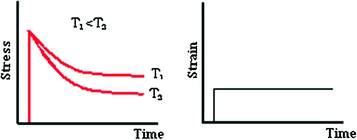

  

  Phenomenon of relaxation for the material for different temperatures

  Fig. 7

  

  Creep phenomenon for the material

• (c) a superimposed behaviour of finite plasticity responsible for the hysteresis phenomena which are independent of the strain rate associated to the relaxed equilibrium states (see Fig. 8) and

  Fig. 8

  

  Phenomenon of hysteresis in load and unload cycles of a reinforced elastomer

• (d) a damage response (stiffness reduction) within the first cycles, which induces in the material a considerable amount of stress softening (the phenomenon known as the Mullins effect—see Fig. 9).

  Fig. 9

  

  Idealized behaviour of the Mullins effect

Although the Mullins effect takes place with the first and more severe load events, it can influence significantly the long-term behaviour of a reinforced rubber [14]. The dependence of the stress–strain response in the pre-conditioning implies that each material point in the non-homogenous deformed component exhibits different stress–strain behaviour. Although all these material points can behave more or less according to a hyperelastic constitutive law, such a particular law varies from point to point. Because of this, a single hyperelastic constitutive law probably cannot provide realistic predictions. The inclusion of the Mullins effect allows load and unloading events to be modelled accurately [15].

The basic response under finite elastic tension governs the response of the vulcanized elastomeric polymers and has been widely investigated as much experimentally [16–19] as theoretically [20–24], and numerically [25–28]. As a result of all these investigations, there is a wide variety of constitutive models which enable the hyperelastic behaviour of elastomers to be modelled through different equations for the strain energy density function [18, 27, 29–31]. These functions are usually restricted to isochoric deformations (that is, deformations that maintain the volume) and are generally formulated in terms of principal stretches or of strain tensor invariants, assuming an isotropic behaviour of the material.

The viscoelastic response is evident in relaxation or creep tests as well as in load cyclic processes. These last show the typical frequency-dependent hysteresis in which the width of the hysteresis cycles increases with the applied deformation. This phenomenon can be explained, from a microscopical point of view, as a rearrangement of the secondary weak bonds among the polymer chains during the strain process. Experimental research works are reported in Ferry [32], Hauser and Sayir [33], Johnson et al. [34] and Lion [8] and other works of a theoretical and computational nature in Simo [35], Kaliske [36] and Lion [8] and Holzapfel et al. [37].

The strain-rate independent elastoplastic response, can be identified as hysteresis in the relaxed equilibrium response within the cyclic deformation process [38] and can be attributed, from a micromechanical point of view, to the processes of irreversible sliding occurring among the reinforced particles and also with the polymeric matrix [39, 40]. This behaviour results in the appearance of residual or permanent strains in the reinforced elastomers subjected to deformation [37]. This phenomenon is known in the industry as permanent set (see Fig. 10).

Fig. 10

Schematic representation of the permanent strain (Lo-Ls)

The effect of damage independent of the strain rate is identified with the stress softening that reinforced elastomers suffer during the first load cycles, known as the Mullins effect [41–45]. From a micro-mechanical point of view this can be explained as the rupture of the bonds among the polymer chains and the reinforced particles [46–48].

The Mullins effect can be interpreted as an effect of damage [49, 50], in which the evolution of the damage depends on the maximum stretch occurring in the strain history [37] or on the maximum strain energy [35, 51, 52]. The energy required to cause the damage is not recoverable and is dissipated in the form of heat.

The constitutive models available in commercial finite element (FE) codes for the modelling of hyperelastic behaviour of elastomeric materials are calibrated from experimental data coming from uniaxial deformation modes. It is highly desirable that the material be tested under uniaxial deformation modes similar to those predominant in the component in order to achieve an accurate characterization.

These hyperelastic models, well known and widely used in the industry, at least in the automotive sector, are insufficient to model the dynamic behaviour of such materials. Although there are other viscoelastic or damage models implemented in FE codes for reproducing the inelastic effects of these materials, it has been demonstrated that they are not able to model accurately the global behaviour of reinforced elastomers.

The dynamic properties of reinforced elastomers are frequency as well as amplitude dependent. Different experimental testing shows that the viscoelastic and elastoplastic properties of this type of material can be independently modelled, and therefore the combination of a viscoelastic and an elastoplastic model in parallel results in a material model, which sums the elastic, viscous and frictional forces. The overlay method, initially proposed by Austrell [53] and Austrell et al. [54], is based on the sum of stress contributions from simpler constitutive models. Originally, this fraction model was proposed by Besselling [55] and was used for modelling the plasticity and creep phenomena in metals. The basic concept of this model is that it considers that the material can be divided into a number of parallel fractions, each with conventional simple properties. The complex behaviour of the material is achieved by the combination of the constitutive simple models and appropriate material parameters. The overlay method allows the dynamic behaviour of reinforced elastomers to be reproduced with a certain degree of accuracy, including the amplitude dependency [56, 57], frequency dependency as well as the mechanical hysteresis typical of this kind of material. Olsson and Austrell [58] propose a procedure for the fitting of the constants of the overlay method from dynamic stationary shear tests. Ahmadi et al. [59] propose a methodology for calibrating the material parameters of the overlay method from quasi-static experimental data.

Anti-vibration components are usually made of reinforced elastomers and work under a preload to which a cyclic strain history is superimposed; dynamic stiffness and the loss angle are essential properties defining their behaviour. Therefore, their prediction with a degree of accuracy is quite important at their design stage.

The model of Morman et al. [60], implemented in commercial FE codes such as ABAQUS [97], MSC. MARC [61] for the analysis of low-frequency vibrations in viscoelastic solids submitted to a initial static strain, is not able to model the behavior of reinforced elastomers. These materials show a strong dependency of the dynamic stiffness with the amplitude [56, 57] but the model only includes the frequency dependency and does not reproduce the dependency either with the preload or with the amplitude.

In practice, there is not too much information available about the dynamic response of reinforced elastomers under complex deformation modes and neither there is any accepted methodology for the consideration of their properties in FE analysis for the prediction of dynamic behaviour under cyclic loads. The methodology used to date consists of the characterization of dynamic properties of the material through testing, scanning a frequency range, average deformations and amplitudes, resulting in a huge matrix with stiffness modulus and loss angle values for each of the analyzed conditions [62]. The analyst must decide which conditions to simulate, depending on the range of values and the design of the applications.

Gómez and Royo [63] developed a methodology which permits considering these dependencies by modifying the viscoelastic model implemented through calibrating the viscoelastic parameters and by defining the material behaviour in a particular way for each element of the model in function of its strain level, preload as well as amplitude. This methodology is based on the combination of the results analysis derived from the material characterization testing and the implementation of the shift factor functions in commercial FE codes, through user subroutines.

Concerning the fatigue life prediction of elastomeric materials, designers define this fatigue life through minimising the stress, strain or energy density values, which are calculated through the FE method, making exclusive use of hyperelastic material models. The inelastic effects, characteristic of this type of material, are not taken into account. The main requirement is to obtain material constants that describe the material behaviour in service conditions. These constants are frequently unknown. In the particular case of elastomers, there remain many unresolved questions, which converge in this simple requirement. The properties of elastomers are strongly dependent on several factors such as the temperature, humidity, light and load conditions to which they are submitted. All these factors are able to modify the fatigue properties of the material (crack initiation and propagation), and therefore the first challenge is to test and asses these properties accurately, quickly and efficiently. The second, more complex challenge is to predict the life through numerical models. Furthermore, being able to simplify the in-service conditions in the experimental testing is important so that the tests may be viable in cost and duration.

The phenomenon of fatigue is described by Ellul [64] as the progressive weakness of several physical variables, i.e. stiffness loss, as the result of the slow growth of cracks produced by the application of cyclic loads or strains. The microscopic process that starts fatigue in elastomers is not so well known as that of metals, and consequently the macroscopic and phenomenological approach remains the most common today. In fact, fatigue treatment in elastomers is mainly empiric. The problem is faced through durability testing in components or in simple samples, whose results are extrapolated for fatigue predictions. This practice is quite limited due to the large number of factors affecting the fatigue life of this type of material, including mechanical factors such as frequency, load sequence, load type—relaxing or nor-relaxing load, uniaxial or multiaxial loads, … -, thermal factors such as temperature, oxygen concentration, ozone, UV rays; and chemical factors such as material composition, additives and vulcanization. Up to now, the consideration of all these factors in damage models for rubber materials has been achieved by means of the calibration of empiric equations to test results. Several authors such as Lake [65, 66], Cadwell [67] and Roach [68] have studied several of the aforementioned aspects. It is important to remark that fatigue failure in elastomers occurs in a fragile way, that is, without previous plastic deformations, as was indicated by Lake [69] and Lake and Yeoh [70]. It occurs in two phases: the first, in which the cracks start nucleation around agglomerate particles in the material, and the second one in which the cracks start growing until the material fails. For some time, it was believed that the crack nucleation, growth and final failure could be modelled in terms of the mechanical behaviour of elastomer fracture [71, 72]. However, there are aspects that only occur during the nucleation phase which require more careful study. In particular, it is necessary to understand the aspects of the multiaxial fatigue in the crack nucleation phase [73].

One of the weak points relating to fatigue life prediction in elastomers is the determination of the accumulated damage and the treatment of multiaxial loads. Flamm et al. [74] demonstrate that, in most cases, the Miner’s linear accumulation damage rule is inadequate. Besides, an added problem is related with the testing frequency, especially for bulk samples, in which the heat generated with the cyclic loading causes degradation of the material. Therefore, the testing temperature becomes an influential factor especially important in the fatigue life of a reinforced elastomer.

The non-linear behaviour of rubber (finite strains and quasi-incompressibility) and the fact that scalar criteria make no reference to a specific material failure plane imply that it is always possible to construct a non-proportional multiaxial history that holds the scalar equivalence criterion value constant while simultaneously varying the individual components of the history [75, 76]. Therefore, scalar equivalence criteria predict infinite life under certain kinds of non-proportional cyclic loading which in fact result in finite life. It can therefore be concluded that an analysis approach that makes specific reference to the failure plane is needed.

Due to the aforementioned limitations of scalar fatigue criteria, different multiaxial fatigue criteria have been proposed in literature to overcome these limitations. However, it is worth pointing out that their level of development has been uneven since most of them have been applied to natural rubber at specimen level only, excepting the cracking energy density proposed by Mars [72] that has been applied successfully to automotive components [77].

The influence of non-relaxing cycles hinders crack growth and therefore increases the expected fatigue life (see Fig. 36). The effect of non-relaxing loads is of great importance in real components such as shock absorbers, which are submitted to static preload (because of the assembly process, external loads or vehicle weight) superimposed on small periodic oscillations. The effects of non-zero minimum loading on fatigue crack growth have been analysed in the literature for strain crystallizing rubbers [78, 79] and for non-crystallizing rubbers [80]. The effects of non-relaxing cycles were incorporated in a fatigue life prediction model using the model proposed by Mars and Fatemi [75, 76].

Relating tribology in elastomers, it is extremely important to develop a scientific knowledge on tribological behaviour on microscale and even more at nanoscale levels in order to avoid expensive “trial and error” method, broadly used in industry. Historically, the majority of friction investigations have been carried out for metals, being the most significant those proposed by Coulomb and Amonton (see [81] and [82]). In contrast with other rigid materials, friction of rubbers is characterized by several macroscopical dependencies: contact pressure, relative sliding speed and temperature. The particular mechanical characteristics of rubbers influence their frictional behavior, as has been demonstrated by many authors [83, 84]. Thirion [85] demonstrated that rubber friction coefficient falls markedly when the contact pressure increases. The surface morphology of the countermaterial also plays a fundamental role in rubber friction. According to most recent investigations found in the literature [86, 87], dry friction on rubbers is mainly governed by the hysteretic and the adhesion phenomena, which can be modelled according to the bulk properties of the rubber material (complex modulus) and the surface roughness structure of the metallic counterpart. Regarding wear in elastomers, there is still not a clearly set up classification. The most general classification of wear types is set up along several decades by authors such as Kragelskii [88], Blau [89], Zhang [90] and Myshkin [91], including in it wear by abrasion, by erosion, by fatigue and by adhesion, although other types of wear such as corrosion, tribochemical or fretting wear, caused in the process during the first wear types, are also considered in literature (Burris [156], [92–94]). The different influences set up in the wear process in the elastomer must also be included in the wear modelling. The vast characterisation was carried out by Meng and Ludema [95], considering three main approximations about wear modelling: models based on empirical relationships, models based on contact mechanics and models based on material failure mechanisms.

1.2 Overview of Mechanical Behaviour of Elastomeric Materials: Elastic, Inelastic and Fatigue Behaviour

1.2.1 Elastic Behaviour

The most obvious as well as the most important physical feature of elastomers is their capacity of being deformed under relatively small stresses. The most relevant features of the elastic behaviour of these materials are as follows [17]:

• (i) The stress–strain curve is highly non-linear and therefore it is not possible to define the elastic behaviour of these materials through the Young modulus (Hooke law) as in metals. In this type of material, the elastic modulus is dependent on the strain level [96]. At low strains the modulus is high because the connections between the reinforcement particles and the matrix are active. As the strain level increases, this property decreases because the interactions between the reinforcement particles break and for high strain levels, the modulus increases again because of the reaction caused by the finite extensibility of the polymer chains.

• (ii) The material, depending on its composition, is able to reach high strains under relatively small loads.

• (iii) The behaviour of these materials is practically elastic, that is, once the stress is removed, the elastomeric material recovers its original shape. This property is more or less true depending on the composition of the elastomer compound. Depending on the added reinforcement particles this property can decrease and the material can exhibit the so-called permanent set or residual strains, which reduce the ability of the material to recover itself.

The non linear elastic behaviour of rubber can be successfully modelled by means of the hyperelasticity models available in commercial FE codes [97].

In general, the compressibility of elastomers is quite low. A material is defined as incompressible when its volume does not vary as it deforms, except for when the deformation is due to thermal expansion.

Elastomers can be considered as incompressible material, because they show a big difference between the initial shear modulus ($\mu_{0}$) and the initial bulk modulus ($K_{0}$). A typical reinforced elastomer for industrial purposes presents a shear modulus ranging between 0.5 and 6 Mpa and bulk modulus ranging between 2000 and 3000 MPa [98]. The high volumetric compared to shear stiffness indicates a practically incompressible behaviour.

The relative compressibility of a material can be evaluated by the relationship ${\raise0.7ex\hbox{${K_{0} }$} \!\mathord{\left/ {\vphantom {{K_{0} } {\mu_{0} }}}\right.\kern-0pt} \!\lower0.7ex\hbox{${\mu_{0} }$}}$. This expression can also be expressed in terms of the Poisson coefficient through (2).

$$ \nu = \frac{{3{\raise0.7ex\hbox{${K_{0} }$} \!\mathord{\left/ {\vphantom {{K_{0} } {\mu_{0} }}}\right.\kern-0pt} \!\lower0.7ex\hbox{${\mu_{0} }$}} - 2}}{{6{\raise0.7ex\hbox{${K_{0} }$} \!\mathord{\left/ {\vphantom {{K_{0} } {\mu_{0} }}}\right.\kern-0pt} \!\lower0.7ex\hbox{${\mu_{0} }$}} + 2}} $$

(2)

Some investigations [99] have demonstrated that natural rubbers reinforced with carbon fibres, when submitted to different load conditions (uniaxial, hydrostatic, monotonic, cyclic), suffer from volume changes. The mechanisms of volume change seem to be related with the damage evolution, chain orientation and viscoelasticity. At the microscopic scale, thanks to observations with the scanning electron microscope (SEM), the evolution of the damage with the elongation has been measured and it has been concluded that, the volume change and the damage evolution are proportional.

1.2.2 Inelastic Behaviour

The response of elastomeric materials under cyclic loading is of interest for several applications, especially those related to the absorption and reduction of vibrations (i.e. for shock absorbers, bumpers and silent-blocks) [100]. Under dynamic loading elastomers exhibit dissipative phenomena such as the Mullins effect, hysteresis and strain-rate dependency due to viscoelasticity.

The parameters usually used for describing the dynamic properties of these materials are the dynamic modulus and the loss angle. These parameters come from the linear viscoelasticity theory.

Suppose that the excitation load A and the response, F, vary in a sinusoidal way:

$$ A = A_{0} sin(\omega t)\,\,\,\,\,\,\,\,\,F = F_{0} sin(\omega t + \delta ) $$

(3)

where, $A_{0}$ and $F_{0}$ are the amplitude of the excitation (displacement) and of the response (force), respectively, $\omega$ is the oscillation frequency and $\delta$ is the delay between the application of the excitation and the system response.

With these magnitudes, the two parameters defining the dynamic behaviour of the material are:

• the dynamic stiffness, defined as the relationship between the amplitudes of the response and the excitation

  $$ K_{din} = \frac{{F_{0} }}{{A_{0} }} $$

  (4)

• the damping, which is related to the delay introduced into the system by the damper element

  $$ \eta = \tan \delta. $$

  (5)

Similarly, instead of relating displacements and forces, stresses and strains are related and the following expressions are obtained for the dynamic modulus

$$ E_{din} = \frac{{\sigma_{0} }}{{\varepsilon_{0} }} $$

(6)

and the damping:

$$ \eta = \frac{{W_{c} }}{{\pi \sigma_{0} \varepsilon_{0} }} $$

(7)

where $W_{c}$ is the energy dissipated in one cycle (see Fig. 11).

Fig. 11

Hysteresis cycles with linear behaviour (left) and non-linear behaviour (right)

These expressions are quite simple to obtain when the behaviour of the model is fully linear and are useful for showing clearly the physical meaning of the two magnitudes. However, their extension to non-linear behaviour, as occurs in real components, is not so easy, due to the fact that harmonics deform the time signal making the measurement of the amplitude as well as the loss angle difficult [101]. The sources for non linearities can be geometrical effects (friction and large displacements), type of loading or material properties, and in the case of reinforced elastomers all these factors at the same time.

Many rubber industrial components suffer from a large variety of dynamic load types, including non-regular periodic oscillations resulting from a combination of different frequencies, pulses and random noise. Together with the non-linear properties of reinforced elastomers, this means that the linear viscoelastic theory cannot be applied [102, 103].

Viscoelastic damping has a significant presence in many polymeric materials and this internal damping is a very useful feature in many industrial components. It has its origin in the molecular structure of the material. The damping comes from the relaxation and recovery of the polymeric net after deformation. An important relationship exists between the effect of the frequency and the temperature because of the direct connection existing between the material temperature and the molecular movement.

The damping grows with the active presence of reinforcement additives which result in a two-phase material with constituents of very different mechanical properties. The phenomenon derives fundamentally from two mechanisms [53]:

• Viscous, a result of resistance to the reorganization of the rubbery phase chains. This reorganization of very long chains cannot occur suddenly. It depends on the strain rate causing the viscous nature of the material.

• Hysteretic, caused by the additives that are much stiffer than the rubber matrix in which they are embedded. These compounds make connections inside the rubbery net. When the material is submitted to strain, these C–C and C-rubber joints break, a process that is rate independent (frequency non-dependent). These breakages are responsible for the non-linear behaviour with the amplitude.

During a load cycle elastomers dissipate energy causing hysteresis. This means that the material behaviour is different during the load path than during the unload path. The hysteresis is a direct consequence of the viscoelastic behaviour of the elastomers and it provokes a delay between the stress and the strain history. The reason that the stress, for a certain strain, is lower during the loading paths is that the material relaxes during the time of the cycle and dissipates energy in the form of heat. This dissipated energy in the cycle corresponds to the closed area in-between the loading and unloading paths and it is used in the industry, for instance, for the damping of vibrations.

The lost energy per cycle W_c (represented by the area enclosed in the cycle) for a certain frequency is expressed as:

$$ U_{c} = \oint {\sigma d\varepsilon = \sigma_{0} \varepsilon_{0} \omega \int\limits_{0}^{T} {\cos (\omega t)} } sin(\omega t + \delta )dt = \pi \sigma_{0} \varepsilon_{0} sin\delta = \pi A_{0} F_{0} sin\delta $$

(8)

where $\varepsilon_{0}$, $\sigma_{0}$, $A_{0}$ and $F_{0}$ are the amplitude of the strain, the stress, the displacement and the force, respectively and $\delta$ is the loss angle, which is related to the material damping by (5).

When non-linear behaviour is present, the hysteresis cycles are deformed from the ellipsoidal shape that they exhibit when non-linearities exist. Usually in these cases the equivalent damping is identified as the area enclosed by the distorted non-linear cycle (see Fig. 11 with (8)).

When reinforced elastomers are submitted to cyclic loading, from the first, until the fourth or fifth cycles depending on the compounding, they suffer from significant stress-softening. This is known as the Mullins effect [104]. When these materials are submitted to large strain cycles, they suffer from stress softening, but only for the subsequent strains lower than those reached previously [105]. After this softening and for strains higher than the maximum strain level reached previously, the material tends to retake the stress–strain behaviour of the virgin state. This phenomenon is attributed to the progressive breakage of the connections between the rubber matrix and the reinforcement particles, and to the configuration changes of matrix itself [53]. The Mullins effect can have important implications for the way in which characterization tests are carried out because the material behaviour can be considerably affected by the previous testing that it has been subjected to [96]. In order to obtain stationary behaviour in the testing of reinforced elastomers, it is necessary to pre-strain the samples before executing the tests, a practice commonly known as material preconditioning.

The anisotropy of an elastomer is strain driven [31, 41] and it is usually defined by the model proposed by Spencer [106] in which the strain energy density function ($W$) includes the predominant behaviour directions through one-dimensional arrays (${\mathbf{m}}_{i}^{0}$ and ${\mathbf{n}}_{i}^{0}$): $W = W\left( {{\mathbf{C}},{\mathbf{m}}_{i}^{0} ,{\mathbf{n}}_{i}^{0} } \right)$. This formulation has been used by different authors to define the behaviour of soft biological materials reinforced with collagen fibres as blood vessels [107], ligaments [108] or cornea [109].

The use of reinforcement loads or particles increases the damping as well as the stiffness of the rubber compound and, as has been previously mentioned, the stress–strain behaviour becomes non-linear, the stiffness being greater at lower strain amplitudes. This phenomenon is known as the Fletcher-Gent effect or Payne effect [57]. The loss angle is also amplitude dependent and reaches its maximum value at a low strain percentage, while decaying considerably for higher strain amplitudes. This amplitude dependency of the dynamic properties makes the linear viscoelasticity theory non valid: the higher the percentage of the reinforcement load, the less applicable is this theory. A feature especially relevant for the isolation of vibrations at high frequencies (usually associated to small amplitude vibrations) is that the dynamic stiffness value tends asymptotically to a finite value at small amplitudes [110].

An additional difficulty induced by the use of reinforcement particles is that the dynamic properties experience a delay in reaching the stationary or equilibrium state after the application of a sinusoidal strain [56]. If the previous deformation is lower or null compared to the measurement strain, the dynamic stiffness will decay until the equilibrium state, while if the previous strain amplitude is higher, there will be a recovery towards the dynamic stiffness associated to the lower strain. This fact suggests that a complete constitutive model for reinforced elastomers requires frictional as well as viscoelastic elements.

Medalia [111] provides a detailed review of the dynamic properties of reinforced elastomers and their dependency with the strain amplitude.

For most industrial applications of reinforced elastomers, the Payne effect, the time dependency as well as the Mullins effect are non desired but unavoidable phenomena. It is therefore desirable to be able to quantify them.

1.2.3 Fatigue

When mechanical rubber components are submitted to dynamic loading, they suffer from fatigue. This phenomenon appears in this type of material as the progressive weakness of several physical variables, i.e. stiffness loss as the result of the slow growth of cracks produced by cyclic loads or strains. There is evidence that the fracture of rubber materials occurs through the presence of defects or imperfections in the parts. From these imperfections, intrinsic in these materials, the cracks can grow under a certain load till they reach a sufficient size to cause the fracture of the material. Due to the initiation of cracks being produced from very small defects in the parts and to the complex behaviour of the elastomeric materials, there is a wide disparity in the prediction of the fatigue life in samples without predefined cracks.

Typical models for predicting fatigue life in rubber follow two overall approaches. The first one focuses on predicting crack nucleation life, given the history of quantities defined at a material point, in the sense of continuum mechanics. Stress and strain are examples of such quantities. The other approach is based on ideas from fracture mechanics, focusing on predicting the growth of a particular crack, given the initial geometry and energy release rate history of the crack.

The crack nucleation approach or ε-N approach considers that the material has a life determined by the stress and strain history at a certain point. The fatigue life according to this approach could therefore be defined as the number of cycles necessary to obtain a crack of a certain length. This approach is quite familiar and convenient for designers as it is formulated in terms of stresses and strains. It is particularly appropriate when the component under study exhibits cracks or initial defects of a size several orders of magnitude lower than its characteristics and when the multiaxial stress state can be related with some accuracy with the stress state of the fatigue material characterization tests. In order to model the effect of the multiaxial loads on the fatigue life of elastomers during the nucleation phase, it is necessary to refer to an equivalence criterion that defines the basis on which to confirm if a component is valid or not for standing fatigue loading and involves one or more parameters characterising the mechanical severity of the load history. The parameters traditionally used in the crack nucleation approach as equivalence criteria are the maximum principal strain and the strain energy density. To date, it seems that only scalar equivalence criteria have been applied for the fatigue life prediction in elastomers, which cannot account for the crack growth direction.

Critical plane theories rely on the physical process of fracture and make use of the continuum variables on the actual fracture plane. Many critical plane approaches have been successively developed in the metal fatigue field, for instance, the models of Brown–Miller [112], Fatemi–Socie [113], Smith et al. [114], Wang and Brown [115–117] and Chen-Xu-Huang [118]. However, for rubber fatigue only a few authors have published crack nucleation parameters associated with a critical plane idea [75, 76, 119, 120]. The use of strain as a life parameter has advantages since it can be obtained directly from measured displacements. When the strain energy density is used, it is often evaluated using hyperelastic material models based on the strain invariants and therefore it is also based on strains. Strain energy density has been used as a fatigue parameter in metals [121], although the correlation between experimental and predicted results is not satisfactory. Rivlin and Thomas [122] proposed a model to study the fracture of rubber under static loading based on the strain energy density, and this has been used by many researchers to correlate analysis results to experimental component life data, considering the strain energy density as a measurement of the energy release rate of the different flaws present in the material. The application to components of this approximation carried out by some authors [123, 124] shows differences in fatigue life to computed strain energy density levels. The main limitations of the strain energy density are that (a) it is unable to predict the fact that the crack surface appears in a specific orientation, and only part of the total spent energy plays a role in the crack nucleation process for multiaxial conditions; (b) it does not account for crack closure and (c) it fails to predict large life differences between simple tension and simple compression loadings. Stress has rarely been used as a fatigue life parameter in rubber [125]. This is related to the fact that fatigue testing in rubber has traditionally been carried out by displacement control, and the accurate stress determination in rubber components can be difficult. The maximum principal strain and the octahedral shear strain have also been used as fatigue parameters based on strains. The maximum principal strain criterion was introduced by Cadwell et al. [67] for unfilled vulcanized natural rubber and remains in use nowadays, particularly for uniaxial strain loadings. It also provides a good correlation for axial/torsion tests, whereas the octahedral shear strain criterion makes a prediction that is roughly similar to the principal strain criterion for rubber [75, 76]. However, for an incompressible material both strain based criteria always satisfy that their values are positive and they are therefore unable to account for compression states where the crack is closed.

The complementary focus to the ε-N approach for the fatigue life prediction of reinforced elastomers is fracture mechanics Lake [69]. This approach assumes explicitly the existence of cracks or defects (material inhomogeneities, agglomerates or contaminants introduced in the material mixing procedure) in the material. The fundamental hypothesis is that the crack growth occurs because the stored potential energy of the component turns into surface energy associated with new crack surfaces. The basis of the energetic approach is the use of the strain energy relaxation velocity or tear energy (T) as a mean of characterizing the behaviour of the crack growth in the material. Usually, this relationship is obtained experimentally through crack growth testing in samples where, for a known strain deformation mode, the tear energy is a function of the sample geometry and/or applied load. With this process together with quantifying the crack growth speed through the applied load cycle, it is possible to characterise the crack growth speed in the material. This approach was successfully applied by Lindley and Stevenson [126] and Gent and Wang [127] for predicting the fatigue behaviour of elastomeric components submitted to compression and shear loads by relating the energy release rate with the strain energy density instead of with the maximum principal strain. However, there remains much to investigate in relation to the suitable material characterization for crack growth, influential factors (initial crack growth, temperature, frequency and load type) and equivalence criteria, which become essential aspects if FE models are to be used for fatigue life prediction.

Fatigue life prediction for rubber combining the crack nucleation and growth approaches has been applied successfully by different authors [66, 128]. This analysis is based on the integration of a crack growth law relating the crack advance per cycle and the energy release rate or tearing energy. The basis of the energetic approach is the use of the strain tearing energy, as a means of characterising crack growth behaviour. The relationship between the crack growth rate dC/dN and tearing energy T is known as the crack growth characteristic of the material since T is independent of the sample geometry. Typical curves for a natural rubber (NR) compound cycled under relaxing and non relaxing conditions (R-ratio of 0.05 and 0.1) are shown in Fig. 36.

The fatigue life of a certain structure can be considered as the number of cycles necessary for a certain crack present in the material at the beginning of the fatigue process (c₀) to grow up to a critical length (c₁) that provokes the final failure of the component. Given the crack growth behaviour and the energy release rate history, the fatigue life can be computed via the integration of the crack growth law between the correct limits [64]. The fatigue life of any rubber component can be predicted by integrating (9) depending on the energy release rate and its description according to the crack growth behaviour only.

$$ \begin{aligned} N &= \int\limits_{{c_{0} }}^{{c_{1} }} {\frac{dc}{{f\left( {T_{\hbox{min} } ,T_{\hbox{max} } } \right)}}} \hfill \\ N &= \int\limits_{{T_{i} }}^{{T_{f} }} {\left( {\frac{1}{{{\raise0.7ex\hbox{${dT}$} \!\mathord{\left/ {\vphantom {{dT} {dc}}}\right.\kern-0pt} \!\lower0.7ex\hbox{${dc}$}}}}} \right)} \cdot \left[ {\frac{dT}{f\left( T \right)}} \right] \hfill \\ \end{aligned} $$

(9)

The Cracking Energy Density (CED) proposed by Mars [72] rationalizes fatigue life for specific failure planes across a wide range of states, relates physically to the fracture mechanical behaviour of small flaws under complex loading and is well defined for arbitrarily complex strain histories. This parameter accounts for the effect of crack closure, which occurs when the stress state causes compression on a material plane. This fact is of great importance because rubber is most commonly used in applications which experience a compressive load. Mars and Fatemi [75, 76] proposed three different critical plane criteria for its use in the computation of CED, the plane that maximizes the CED peak value, the plane of maximum CED range and the plane of minimum life.

Saintier et al. [119, 120] investigated fatigue crack initiation under multiaxial non-proportional loadings in a natural rubber and tested under multiaxial loading. The proposed fatigue crack criteria is based on the micro mechanisms of crack initiation such as cavitation, decohesion and micro-propagation, consisting of a critical plane approach under large strain conditions using a micro to macro approach. This criterion gives promising results, by predicting the fatigue life, crack orientations and location even in cases with internal crack initiation although for the moment this approach is limited to proportional loading histories.

Verron et al. [129, 130] and Andriyana et al. [131] proposed a new predictor for crack nucleation in rubber based on the configurationally stress tensor to propose a fatigue life predictor for rubber. This criterion is formulated in terms of continuum mechanics quantities in order to be combined with the standard FE method in engineering applications. It takes into account the presence of microscopic defects by considering that macroscopic crack nucleation can be seen as the result of the propagation of those microscopic defects. For elastic materials, it predicts privileged regions of rubber parts in which macroscopic fatigue cracks might appear.

Wang et al. [132] proposed a continuum damage model to investigate the fatigue damage behaviour of elastomers. The elastic strain energy of a damaged material is expressed based on the Ogden model [24], and the damage strain energy release rate is derived in the context of continuum damage mechanics. The damage evolution equation is established to develop a formula to describe the fatigue life as a function of the nominal strain amplitude under cyclic loading. The results indicate that the theoretical formula for the fatigue life as a function of the nominal strain amplitude, derived from the proposed damage model, can describe experimental data for carbon-filled natural rubbers.

1.3 Overview on Tribological Behaviour of Rubber-Like Materials: Friction and Wear

In recent decades, tribology has played a remarkable role in mechanical systems in which components are made of rubber-like materials working under sliding conditions. Such components are important in most industrial sectors, particularly in automotive and railway applications. Two of the main aspects related with the tribology of rubber-like materials are friction and wear, which are explained in detail below.

1.3.1 Friction of Rubber-Like Materials

As it is commonly known, the classical Coulomb and Amontons friction laws, which mainly establish that the friction coefficient is independent of the area of contact, have been proved to be non-valid in the case of rubber-like materials. For this material type, due to their specific mechanical properties, the friction coefficient should be expressed as a function of contact pressure, sliding speed, temperature and lubrication regime.

$$ \mu = \mu \left( {L,T,\dot{\gamma },\upsilon ,R_{a} \ldots } \right) $$

(10)

The dependence with the contact pressure is associated to the varying ratio of real (microscopic level) to apparent (macroscopic level) area of contact when the vertical load (contact pressure) rises. The problem increases in complexity when neither the contact pressure distribution nor the ratio of real to apparent area of contact are uniform along the apparent area of contact, cylindrical contact geometry being a typical example of this situation.

In the proposed expression (10), several dependencies on external parameters such as vertical load (contact pressure), temperature, sliding speed, etc., are introduced as key variables. Rubber-like materials in general and rubbers in particular have high friction characteristics, a consequence of their low elastic modulus and their viscoelasticity. Thus, under contact pressure they deform to a large extent, resulting in high values of the real area of contact. Hence, classical models for metals are no longer valid in the case of rubber friction.

The high friction coefficient has been exploited in many applications, for example: tyres, shoe soles, bicycle brake blocks, etc. However, there are many other applications in which the frictional behaviour of the rubber is expected to have the opposite characteristics, as for example in the case of windscreen wipers and seals. In such cases the rubber must be treated to produce low frictional properties in the case of dry friction, or else the working conditions must be ensured to be in the hydrodynamic lubrication regime.

It is commonly known that friction coefficient values are difficult to find in the literature. This is because the friction coefficient can rarely be assumed to be constant and, as stated in expression (10), it depends on several factors such as contact pressure (vertical load), sliding velocity, temperature, surface roughness and lubrication regime, where applicable.

As described in the Sect. 1.2, Amontons and Coulomb established that friction force is proportional to the vertical load and independent of the geometry of the contact. Coulomb defined the friction coefficient μ as the ratio between friction and vertical load. For materials obeying this law, μ is independent of the vertical load and thus of the normal stress. Rubber does not obey Amontons’ and Coulomb’s laws since the friction coefficient falls markedly when increasing normal stress. For this particular behaviour, an analytical law which became widely used was defined by Thirion [85]:

$$ \frac{1}{\mu } = a + b\left( \frac{P}{E} \right) $$

(11)

where μ is the friction coefficient, P is the normal stress, E is the elastic modulus of the rubber and a and b are empirical constants. Schallamach [133] later showed how the behaviour described in Eq. (11) may be explained on the assumption that the friction force is proportional to the true area of contact, resulting in:

$$ \mu = const\left( \frac{P}{E} \right)^{{\frac{ - 1}{n}}} $$

(12)

where the value of n is derived from a model which considers the deformation of the rubber on the asperities of the metallic counterpart and depends on the geometry and distribution considered for peaks and valleys. In general, n depends on the nominal normal stress, but for restricted ranges it is considered to be constant. At sufficiently high normal stresses, the real area of contact becomes equal to the apparent area of contact, so that the frictional force becomes constant and μ is inversely proportional to P, as described in (12). This particular condition is referred to as “saturation”.

In addition, the lubrication regime plays a substantial role in the frictional behaviour of rubbers in lubricated (fluid) conditions. The influence of the lubrication regime can cause a drop in the friction coefficient value from one order of magnitude, depending on whether the lubrication regime is in the boundary state (direct interaction between the rubber and the micro-asperities of the metallic counterpart), the elasto-hydrodynamic state (the rubber and the asperities of the counterpart are separated by the lubricant placed in between, and the frictional force is caused by the viscous shearing of the fluid) or finally in the mixed regime (the lubricant thickness is of the order of a couple of molecular chain lengths). The influence of the lubrication regime on friction is described by the Stribeck curves (see Fig. 12, [84]), which establish a relationship between the lubrication regime and a given physical magnitude consisting of the ratio of lubricant viscosity times sliding speed to vertical load.

Fig. 12

Variable dependency in friction between rubber-like materials and wear

The first stage of the curve corresponds to boundary lubrication (BL), the second to mixed lubrication (ML) and the third to elasto-hydraulic lubrication (EHL). In the curve, μ is the friction coefficient, υ the kinematic viscosity of the fluid, $\dot{\gamma }$ the sliding velocity, F_N the normal load and h_film the height of the fluid film.

Finally, prior to the definition of a test configuration for the analysis of the friction coefficient in rubber-like materials, the micro-scale effects on their friction mechanisms briefly described above must be taken into account. Thus, within the experimental and numerical work to be carried out for the definition of the test configuration, the effect will be evaluated of the macroscopic parameters (vertical load, sliding speed and temperature) on the measured friction force.

1.3.2 Wear on Rubber-Like Materials

Wear in polymers in general and in rubber-like materials in particular is defined as the damage done to a solid surface, involving progressive material loss and caused by the relative movement between contacting surfaces. Some authors, such as Zhang [90], exclude from the category of wear the fracture or fatigue damage caused by inner cracks of the solids, the pure corrosion or aging of rubber surfaces resulting from chemical reactions and plastic deformation without loss of material. Wear depends on several factors, such as the nature of materials at the surface zone as well as in the bulk far from the contact zone, on operating parameters, on geometry at both macroscopic and microscopic level, and on environmental conditions. Surveys carried out by Rymuza [134], Viswanath and Bellow [93] and Stachowiak and Batchelor [82] show several dependencies of different variables in the dynamics of wear between rubber-like materials and metals, as illustrated in Fig. 13.

Fig. 13

Variable dependency in wear between rubber-like materials and metals

The influence of the most relevant parameters is detailed below.

1.3.2.1 Formation of a Material Transfer Layer in Contact Pair

Several authors have examined transfer layer formation in the sliding of a rubber-like material over a counter material with a harder contact surface. A notable example is the study performed by Buckley [135] with polytetraethylene (PTFE) sliding over a metallic surface, where a strong adhesion between both materials is produced, caused on the one hand by the chemical reaction between fluorine and carbon from PTFE with the metallic counter surface, and on the other hand by the ease of movement of the material molecules under load conditions. Other authors, such as Makinson and Tabor [136] and Tanaka et al. [137], have analysed the transfer mechanism of this material and other materials such as high density polyethylene (HDPE) and ultra-high molecular weight polyethylene (UHMWPE), observing a discrete sheet formation of material over the metal, producing wear increase and friction decrease.

In other research, such as that carried out by Thorpe [138], the material was detached at the asperity zones separately and stuck over the counter surface in a material transfer type known as lump transfer.

According to analyses by Jain and Bahadur [139], a similar behaviour is produced in the contact between two rubber-like materials, setting up a material transfer layer in the material with the weaker cohesion.

1.3.2.2 Influence of the Counter Material Roughness

Several authors have focussed their studies on the analysis of sliding contact pairs between rubber-like materials and metals to obtain the optimum material roughness which generates the lowest material wear. On the one hand, authors such as Birkett and Lancaster [140] suggest that the lower the counter material roughness, the lower the wear of the rubber-like material. On the other hand, Dowson et al. [141] established an optimum roughness level within the material manufacture tolerances, also depending on the sliding velocity of the application. Other surveys, such as that carried out by Barrett et al. [142] on ultra high molecular weight polyethylene (UHMWPE), established a dependency loss of the roughness with the wear rate at high sliding velocities due to the faster transfer layer formation and also to the wear rate stabilization.

In another study, Stackowiak and Batchelor [82] established the penetration depth of the metallic asperities and the sliding distance as the most influential parameters on the wear rate. According to the same authors, the wear does not remain constant over time. After a fast initial increment of the wear rate, it then decreases over time once the asperities have been covered by the rubber-like material transfer layer.

Another additional factor affecting the wear rate, apart from roughness, is the height distribution in the counter material asperities. Play [143] found important differences in the wear rate between surfaces with a height Gaussian distribution in asperities and surfaces with a non Gaussian distribution. This fact also influences the amount of detached debris, which determines the transfer layer formation modifying the wear rate as well as the friction, as shown by Blanchett and Kennedy [144] and by Barrett et al. [142].

1.3.2.3 Influence of the Temperature

Several authors, such as Tanaka and Uchiyama [145], Kar and Bahadur [146] and Stachowiak and Batchelor [82], have analysed the influence of the temperature in the wear process of rubber-like materials under sliding conditions with metal. The temperature rise of the rubber-like material in the wear process, caused by its low melting point and by its low thermal conductivity, implies a wear process modification in the contact pair, decreasing the friction and increasing the wear rate. This process is known by authors like Stackowiak and Batchelor [82] as melting wear. During this process, the melted rubber-like material is placed on the counter material surface which is not affected by the temperature rise of the rubber-like material because the melting point of the counter material is much higher.

Another influential aspect in the rubber-like material wear process is the latent heat of melting, already analysed by Mc C. Ettles [147] in specimens of polypropylene and nylon sliding over steel. This parameter imposes a limit to the temperature attained at the contact pair, so that although the friction coefficient changes with the sliding velocity or with the load when the melting point of the rubber-like material is attained, the temperature at the contact pair remains constant at the yield limit.

Besides, for soft materials such as aluminium, particles of the counter material can also be transferred to the rubber-like material surface, implying a friction coefficient increase, according to the researches of Mizutani et al. [148].

Thermal conductivity of the material is another influential factor in rubber-like material wear, as shown by Watanabe and Yamaguchi [149] in wear tests with nylon specimens on steel and glass surfaces. For high test velocities and the same test conditions, melting wear is found in nylon on glass, but not on steel, since the thermal conductivity of this material is higher than that of glass.

Finally, the combined effect of counter material roughness and the contact temperature when both parameters have high values causes the wear rate of the rubber-like material to be extremely high, even without reaching the melting point of the material [150]. This was proved by Barrett et al. [142]. In this case, severe abrasion of the rubber-like material surface takes place, beginning with a linear wear rate of shorter periods of higher wear combined with longer periods of less significant wear.

1.3.2.4 Influence of Lubricant and Oxidant Agents

In general, the inclusion of lubricants reduces friction in contact pairs, the quantitative reduction of the friction depending on the type of rubber-like material and on the lubricant. Authors such as Cohen and Tabor [151] have noticed a sharp drop in the friction coefficient in tests with nylon and glass in a water bath, obtaining lower drops in tests with organic substances such as hexane or benzene. The differences are caused by the polar nature of the polyamide, the main constituent of nylon. The formation of a transfer layer is also modified by lubricants, decreasing to very low values under wet conditions, especially under water [152].

The wear rate of the contact pair is also affected by the solubility of the rubber-like material. In some cases, if a solvent is able to penetrate through the rubber-like material surface, an accelerated wear increase with cracking in the rubber-like material surface is produced, mainly caused by the action of the solvent. According to an analysis by Evans [152], several solvents such as acetone, benzene, tetraclochlorinemethane or toluene show solubility parameters near to that of different rubber-like materials, causing an accelerated wear as contact is produced.

Regarding the effects of oxidative agents, some polymers such as nylon or polyethylene show a wear process similar to the corrosive wear of metals, leading to a reduction in friction coefficient values and to an increase in the wear rate. This effect is proportional to the surface damage level due to the corrosive agents. This feature is consistent with the resistance of UHMWPE to chemical agents, observed by authors such as Batchelor and Tan [153] and Scott and Stachowiak [154].

1.3.2.5 Influence of Rubber-Like Material Microstructure

It is worth mentioning, according to studies from Bartenevev and Lavrentev [155], the low friction values and low wear rates at temperature values near the glass transition point, showing high wear rates at different temperatures, higher or lower than that point. This behaviour is different from that of other crystalline polymers, showing a wider temperature range for low friction coefficient and wear rate values.

1.3.2.6 Types of Wear in Rubber-Like Materials

A classification of the wear types in rubber-like materials has not yet been clearly established. Over more than half a century, several researchers including Kragelskii [88] and Blau [89] have proposed several types of classifications from different points of view. However, to date there is no generally recognised methodology. Zhang [90] takes into consideration a classification including abrasive, erosive and fatigue wear, while other authors such as Myshkin et al. [91] include adhesive wear in this classification. These wear types are the most broadly accepted in the literature. In some cases, corrosive or tribo-chemical wear are also considered, as analysed by Burris [156] and Viswanath and Bellow [93], or fretting wear, as studied by Je et al. [92] and by Nah [94]. However, these are taken as particular cases of the most influential phenomena previously referred to. The most relevant wear types are explained in detail below.

• (a) Erosive wear

This is defined as the wear resulting from the interaction between a solid surface and a fluid stream containing abrasive particles at a certain speed. The types of erosive wear can be abrasive erosion, if it is caused by a fluid stream parallel to the solid surface (see Fig. 14a), or impact erosion if it takes place under a fluid stream perpendicular to the solid surface (see Fig. 14b).

Fig. 14

Types of erosive wear. a Abrasive erosion. b Impact erosion

It is important to mention the surveys of Zhang [157, 158] into the wear mechanism by abrasive erosion of rubber-like materials such as natural rubber (NR), styrene-butadiene rubber (SBR), nitrile-butadiene rubber (NBR) or polyurethanes (PU). These surveys were carried out in an abrasive erosion testing machine under wet conditions with sodium hydroxide in water. The effects analysed in these tests by SEM examinations were: delamination, micro cut, micro crack initiation and propagation or mechanic-chemical degradation. Besides, this author also studied the influence of the particle wear speed, flow velocity, particle size and particle concentration for the same rubber-like materials. It is also worth noting the work of Arnold and Hutchings [159] which studied the erosive wear of non-reinforced rubber-like materials, finding two different mechanisms: the first at low impact angles and the second under conditions of perpendicular impact to the surface, eliminating the material from the surface in both cases by means of fatigue crack propagation.

• (b) Adhesive wear

This takes place as a result of the adhesive forces present in the contact pair between two solid surfaces, where part of the rubber-like material is transferred from its surface and adheres to the counter material surface (see Fig. 15). Bely et al. [160] noticed that the material transfer is the most important characteristic of adhesive wear in rubber-like materials. The processes associated with other wear types such as abrasive wear and fatigue wear can also take place together with adhesive wear.

Fig. 15

Adhesive wear

The material transfer phenomenon caused by friction, where micro size particles are transferred from one surface to another, is a very common effect in contact pairs between rubber-like material and metal. This effect was studied by Makinson and Tabor [136] and by Tanaka et al. [137]. Usually, the soft material film, that of the rubber-like material, is transferred to the harder material surface, in this case the metal surface. If the transferred rubber-like material film is continuously being placed and eliminated, the wear rate increases. If, on the other hand, the rubber-like material film is maintained, even with changes in the friction force, the changes in the wear rate vary very slightly. In general, however, it can be stated that a high degree of adhesion is produced in a contact pair in which rubber-like material and metal are involved.

In rubber-like materials with low concentrations of additives in the components, a very slight transfer to the metallic counter surface is produced due to the low adhesion between both surfaces. This fact implies that the contact pair shows very inadequate tribological properties [161]. Under other circumstances, the harder material can be transferred over (onto?) the softer material surface; for instance, bronze may be transferred to rubber-like material. This results in harder material particles being set in the rubber-like material surface, acting as abrasive particles, as analyzed by Myshkin et al. [91].

• (c) Abrasive wear

The wear type known as abrasive wear is the most common in polymers in general and in rubber-like materials in particular. It is caused by the relative movement between a solid surface and sharp particles of the same or higher hardness acting against the surface of the first body. Studies carried out by Swain [162] revealed that indirect mechanisms such as micro cutting, detachment of individual particles of the material or accelerated fatigue by repetitive deformations can be involved in the cutting process of the material (see Fig. 16).

Fig. 16

Abrasive wear

In the wear caused by a cutting mechanism, a very sharp tool or a very rough surface cuts the softer surface, eliminating the material by debris formation. Depending on the material hardness, the debris can be detached as a result of crack propagation or of repetitive deformation of the material [82].

According to Zhang’s [90] surveys, rubber abrasion can be classified into two categories: pattern and intrinsic abrasion. In the first type of abrasion, parallel ridges, called abrasion patterns, appear on the surface at right angles to the sliding direction. Pattern abrasion occurs under unidirectional sliding direction conditions. On the other hand, intrinsic abrasion arises when the direction of the relative motion changes periodically. Usually, and under identical conditions, the wear rate of pattern abrasion is higher than that of intrinsic abrasion. Zhang [90] also classifies abrasion wear into wet abrasion and dry abrasion, depending on whether or not liquid exists on the frictional surface. Another classification made by the same author is based on the type of contact between both surfaces: point contact abrasion, line contact abrasion and multiple-point contact abrasion.

One of the most widespread techniques for observing the wear process in rubber-like materials is by means of electronic microscopy (SEM). Some authors, such as Bhowmick et al. [163], have investigated this process and established that a cutting mechanism at micromechanical level is present, in which the material is eliminated by means of wavy sheets. This process is known as micro-cutting. Kayaba [164] revealed another mechanism involving the formation of grooves along the sliding direction, identified by means of several observations of specimens tested in a tribometer under the pin-on-disc configuration. This mechanism, known as ploughing, is less destructive than micro-cutting and does not involve material being detached, Other authors, such as Myshkin et al. [91], have named this wear type grooving.

In harder materials, such as thermoplastic polyurethanes (TPU), two different mechanisms are present in the wear process: macro-delamination and micro-molecular fracture [165, 166]. Macro-delamination consists of the formation and growth of cracks, leading the material to tear in terms of parallel grooves, finally breaking due to tensile stresses. Micro-molecular fracture consists of the detachment of small particles due to the breaking of simple material molecules or any of its aggregates. At the same time, abrasive wear particles in these materials are also related with the presence of additives, fillets or plasticizers. Bartenevev and Lavrentev [155] noticed that plasticizers have a negative effect on the abrasive wear of several polymers due to their softening.

Zhang [90] has also presented valuable surveys in the quantitative evaluation of rubber abrasion by means of different methods such as fractal theory, computerized simulation technology and computer-generated image analysis.

• (d) Two-body and three-body wear

Abrasive wear is commonly divided in two groups: two-body and three-body wear.

Two-body wear is caused by sharp protuberances present in one of the surfaces which can slide over the second one. In this type of wear, some asperities cause the wear previously referred to as ploughing, while other asperities cause micro-cutting wear, depending on two factors: the attack angle of the particle and the shear stress generated between both contact surfaces [91].

On the other hand, in three-body wear, there are particles trapped in both contact surfaces which can rotate and slide freely between them. These particles are detached from the worn surface of the contact pair or come from the lubrication of the contact pair if the test is carried out under wet conditions. They may also be particles from the environment. The effect, according to research by Singer and Wahl [167], is a decrease in the friction between both surfaces, setting up transfer layers but also inducing wear tracks with the detached particles.

For some time, it was believed that these two wear types were very similar. However, Zum Gahr [168] identified several differences between them. The wear rate in three-body wear is around one order of magnitude lower than that obtained in two-body wear, since the abrasive particles in three-body abrasion wear the contact surfaces only 10 % of the sliding time, while during the remaining 90 % of the time they merely rotate between the surfaces [169]. According to Johnson [170], another difference lies in the fact that two-body wear corresponds to a material elimination model typical of cutting or micro-cutting, while three-body wear involves slower mechanisms of material elimination. In the latter case, the mechanisms common in two-body wear, such as micro-cutting or ploughing, do not occur. There is instead a random wear mechanism due to the non-controlled presence of a third body [171].

• (e) Fatigue wear

This is a type of wear similar to abrasive wear, produced against a rough surface. The difference between them, according to Zhang [90], is that the surface for fatigue wear is formed by small soft rough projections, while for abrasive wear the surface is formed by hard sharp projections. Fatigue wear as a concept was presented by Kragelskii [88], being a low intensity wear type compared with abrasive wear. The main feature of this type of wear is the irreversible damage suffered by the material under the repetitive action of compressive, tensile and shear strains in the contact pair. Along the relative sliding between both surfaces, the polymer interacts with the sharper projections of the rough counter surface, which leads to the initiation and development of cracks, also helped to propagate by the presence of internal voids in the material [169]. Several authors, including Zhang [90], have modified the term of fatigue wear to frictional wear or rolling wear if the rubber-like material shows low tearing resistance and slides over low rough surfaces with a high friction coefficient, causing the formation of rolling or spiral particles at the contact pair. These particles are continuously detached during sliding. In this type of wear, each asperity of the worn material surface suffers a sequential load from the asperities present in the contact. Subsequently, stresses arise at different scales in the surface and subsurface regions. These stresses are the cause of the material fatigue, which leads to the initiation and propagation of cracks and to the formation of worn particles. These cracks are formed at points where the maximum shear stresses occur, their position also depending on the friction coefficient between both surfaces. The higher the friction coefficient, the nearer the point of maximum shear stress to the surface, its depth increasing as the friction coefficient decreases. At the same time, the initiation of fatigue cracks is helped by the presence of defects in the material, such as marks, scratches in the surface, internal voids or impurities. These defects are responsible for the stress concentrations. With the repetitive action of the load and, consequently, of the material stress, the cracks grow, join each other and intersect generating the material detachment [91]. Figure 17 shows the fatigue wear process.

Fig. 17

Fatigue wear. a Crack initiation as result of fatigue process. b Crack growth and propagation and formation of wear particle

Other authors such as Jain and Bahadur [172] or Neale and Gee [173] consider this type of wear as abrasive wear on a small scale since the asperities of the counter surface, at micromechanical level, act as initiating particles of the rubber-like material abrasion. According to analyses by Jia and Ling [174] of fatigue wear in polyurethanes caused by the repetitive action of abrasive particles on the material, and considering that its elastic modulus is within that of a rubber-like and of a plastic material, the effects of ploughing or crack formation are not directly generated. Nevertheless, mechanical fatigue is more likely to take place. According to this study, the repetitive impacts of the abrasive particles with the material lead to tensile, compressive and shear strains and stresses in the contact layer, forming fatigue cracks due to the repetitive actions with the interactions. Other surveys carried out by Liu et al. [175] and by Marchenko [176] show the highest shear stress at a certain depth under the contact surface. On the other hand, the highest material strain is located at the surface, a propitious place for crack initiation although at the same time this is where the highest compressive stresses are also located which in some way act against crack initiation. As the distance from the contact surface increases, the compressive stresses decrease faster than the shear stresses. This means that almost all the stresses are shear stresses which, being cracks, are more easily formed at a distance from the contact surface.

Another effect taken into consideration by Jia and Ling [174] is the temperature influence, which is higher in TPU layers near to contact due to friction and material deformation hysteresis. This heat can be more easily dissipated at the surface where the temperature quickly drops due to the contact with the environment. However, its dissipation is more difficult at a certain depth, and this decreases the cohesive material energy and consequently cracks are initiated. The repetitive contact of these particles implies that cracks propagate and intersect with each other, leading to material being detached as debris. Stackowiak and Batchelor [82] also studied the temperature effect on wear behaviour. They demonstrated that with the low temperature at which polymers melt, as well as their low thermal conductivity, the high temperature reached at the contact pair is higher than the melting point of the material and it thus begins to deform in an effect known as melting prow. This effect, spread over all the contact surface of the polymer, is known by other authors such as Bartenevev and Lavrentev [155] as fatigue wave formation.

Other authors establish in their studies that cracks present in the material subsurface are exacerbated during application cycles by the plastic deformation of the material, being propagated to near cracks in a process defined as delamination by authors such as Johnson [177], Suh et al. [178] and Da Silva [179]. According to these authors, any particle generated and detached in the wear surface implies a higher dragging, thereby increasing the friction force. This in turn accelerates the delamination process.

2 Constitutive Models for F.E. Modelling of Elastomeric Materials

Hyperelasticity refers to the quality of materials which can experience large elastic strain that is recoverable. Elastomers such as rubber and many other polymer materials fall into this category. The microstructure of polymer solids consists of chain-like molecules. The chain backbone is mostly made of carbon atoms. The flexibility of polymer molecules allows different types of arrangement such as amorphous and semi crystalline polymers. As a result, the molecules possess a much less regular character than metal crystals. The behaviour of elastomers is therefore very complex. On a macroscopic scale, they usually behave as elastically isotropic initially, and anisotropic at finite strain as the molecule chains tends to realign in the loading direction. However, under essentially monotonic loading conditions a larger class of elastomers can be approximated by an isotropic assumption, and this has been historically popular in their modelling.

The constitutive behaviour of hyperelastic materials is usually derived from the strain energy potentials. Also, hyperelastic materials generally have very small compressibility, often referred to as incompressibility. The hyperelastic material models assume that the material response is isothermal. This assumption allows strain energy potentials to be expressed in terms of strain invariants or principal stretch ratios. Except as otherwise indicated, the materials are assumed to be nearly or purely incompressible. Material thermal expansion is always assumed to be isotropic.

2.1 Modelling the Elastic Behaviour of Elastomers

2.1.1 Basic Kinematics of Finite Elastic Deformations

This section gives a brief description of the finite strain theory, introducing concepts such as gradient tensors, finite strain tensors, stretch ratios as well as compatibility conditions. For a detailed description of these concepts, see Holzapfel [180].

A body whose configuration in terms of size or shape changes under external loads is defined as a deformable body. A direct result is that distances between points of the solid vary. Therefore, it is appropriate to consider two different configurations of this type of solid, the undeformed configuration and the deformed configuration after applying external loads.

Given a three-dimensional solid deformable body, as shown in Fig. 18, and a Cartesian reference system ($\vec{E}_{1} ,\vec{E}_{2} ,\vec{E}_{3}$), the position vector ($\vec{X}$) for the point P ₀ in the undeformed configuration can be written as:

$$ \vec{X} = X_{1} \vec{E}_{1} + X_{2} \vec{E}_{2} + X_{3} \vec{E}_{3} $$

(13)

Fig. 18

Deformed and undeformed shape for the deformable body

After a load application, the solid body is deformed and the point P ₀ is now in the position P, whose coordinates are:

$$ \vec{x} = x_{1} \vec{E}_{1} + x_{2} \vec{E}_{2} + x_{3} \vec{E}_{3} $$

(14)

The relationship between deformed and undeformed coordinates is the displacement field in the spatial configuration:

$$ \vec{u} = \vec{x} - \vec{X} = u_{1} \vec{E}_{1} + u_{2} \vec{E}_{2} + u_{3} \vec{E}_{3} $$

(15)

From a Lagrangian point of view, the coordinates for points in the deformed configuration can be expressed as a function of the coordinates of points in the undeformed configuration.

$$ \vec{x} = \vec{x}\left( {\vec{X}} \right) $$

(16)

The deformation gradient tensor is defined, based on the relationship between the position vector and the deformed and undeformed configurations, as:

$$ {\mathbf{F}} = \left[ {\frac{{\partial x_{i} }}{{\partial X_{j} }}} \right] $$

(17)

In a deformable body, those properties which change along with the deformation of the body might be described either by the evolution of its value along the trajectory of a given material point, material description (also known as Lagrangian description), or by the change of its value at a fixed location in space occupied by (different for each time instant) particles of the body, spatial (Eulerian) description.

The rigid body motion can be decomposed in a displacement and a rotation. Equation (18) relates the initial and final coordinates of the deformable body:

$$ \vec{x} = R \cdot \vec{X} + \vec{c} $$

(18)

where

$K_{0} = \frac{2}{D}$ :

translation vector (independent of position).

R :

rotation tensor, due to its antisymmetry verifies:

$$ {\mathbf{R}}^{\text{T}} \cdot {\mathbf{R}} = {\mathbf{R}} \cdot {\mathbf{R}}^{\text{T}} = {\mathbf{I}} $$

(19)

In order to separate the movement due to the deformation from the rigid body motion, the right Cauchy Green strain tensor is defined as:

$$ {\mathbf{C}} = {\mathbf{F}}^{\text{T}} \cdot {\mathbf{F}} $$

(20)

If there is only rigid body motion, this tensor is constant and unitary:

$$ {\mathbf{C}} = {\mathbf{F}}^{\text{T}} \cdot {\mathbf{F}} = {\mathbf{R}}^{\text{T}} \cdot {\mathbf{R}} = {\mathbf{I}} $$

(21)

The left Cauchy-Green deformation tensor is obtained reversing the order of multiplication in the formula for the right Cauchy Green strain tensor:

$$ {\mathbf{b}} = {\mathbf{F}} \cdot {\mathbf{F}}^{\text{T}} $$

(22)

The deformations can also be expressed using the Green Lagrange strain tensor defined according to the following expression:

$$ {\mathbf{E = }}\frac{1}{2}\left( {{\mathbf{F}}^{\mathbf{T}} \cdot {\mathbf{F}} - {\mathbf{I}}} \right) = \frac{1}{2}({\mathbf{C}} - {\mathbf{I}}) $$

(23)

This tensor is null when there is no deformation.

When the movement of the solid body is due to a displacement and a rotation, the deformation gradient tensor could be expressed as:

$$ {\mathbf{F}} = {\mathbf{R}} \cdot {\mathbf{U}} $$

(24)

where U is a symmetric tensor called the right stretch tensor, related with the right Cauchy Green strain tensor through the following expression:

$$ {\mathbf{C}} = {\mathbf{F}}^{\text{T}} \cdot {\mathbf{F}} = {\mathbf{U}}^{2} $$

(25)

• (a) Principal stretches

The principal stretch coefficients are now described. Consider two points, P ₀ and Q ₀ , in the undeformed configuration of a deformable body, as shown in Fig. 19, both related by the vector δL. If the body is subjected to a displacement field defined through the deformation gradient tensor F, the displaced points P and Q in the deformed configuration are related by means of the δl vector, and this verifies:

Fig. 19

Deformation for a deformable body

$$ {\mathbf{F}} \cdot {\mathbf{A}} = {\mathbf{R}} \cdot {\mathbf{U}} \cdot {\mathbf{A}} = \lambda \cdot {\mathbf{a}} $$

(26)

where

A :

unity vector of vector δL on undeformed configuration.

a :

unity vector of vector δl on deformed configuration.

$\lambda = \frac{\delta l}{\delta L}$ :

stretch coefficient of vector δL, due to deformation.

Assuming that there are no rotations and δL only changes its modulus due to deformation, then the following conditions are satisfied:

$$ {\mathbf{F}} = {\mathbf{U}} $$

(27)

$$ {\mathbf{A}} = {\mathbf{a}} $$

(28)

Therefore (26) can be transformed into the following expression:

$$ {\mathbf{U}} \cdot {\mathbf{A}} = \lambda \cdot {\mathbf{a}} $$

(29)

Reordering this expression, it is possible to obtain:

$$ \left( {{\mathbf{U}} - \lambda {\mathbf{I}}} \right) \cdot {\mathbf{A}} = 0 $$

(30)

According to (30), A is an eigenvector of U associated to the eigenvalue λ. Since U is a 3 × 3 positive definite matrix, it has three positive and real eigenvalues called principal stretches

$$ \lambda_{1} \ge \lambda_{2} \ge \lambda_{3} $$

(31)

The right stretch tensor U has three principal directions associated to these eigenvalues, forming an orthogonal coordinate system named the principal axis system, where the right stretch tensor adopts the following form:

$$ {\mathbf{U}} = \left[ {\begin{array}{*{20}c} {\lambda_{1} } & 0 & 0 \\ 0 & {\lambda_{2} } & 0 \\ 0 & 0 & {\lambda_{3} } \\ \end{array} } \right] $$

(32)

Observing the right stretch tensor expressed in the principal axis, and considering a displacement field defined through the deformation gradient tensor F, the movement of L ₀ , vector joining two near points in a deformable body, could be decomposed in two parts:

First, a variation of the L ₀ modulus expressed in the principal axis as shown in Fig. 20 $\bar{L}_{f} = \bar{L}_{0} + \overline{\Updelta L}.$

Fig. 20

Principal stretches

The change in modulus for the components of L ₀ is defined by the principal stretches ($\lambda_{1} ,\lambda_{2} ,\lambda_{3}$) since:

$$ \lambda_{i} = \frac{{L_{i} \pm \Updelta L_{i} }}{{L_{i} }} $$

(33)

And second, the movement is completed with a rotation of the L _f vector according to the rotation tensor R.

• (b) Strain invariants

The deformation of a body can be expressed in terms of the right Cauchy Green strain tensor invariants. These invariants are defined as:

$$ I_{1} = C_{11} + C_{22} + C_{33} $$

(34)

$$ I_{2} = C_{11} C_{22} + C_{22} C_{33} + C_{33} C_{11} - C_{12}^{2} - C_{23}^{2} - C_{31}^{2} $$

(35)

$$ I_{3} = C_{11} C_{22} C_{33} + 2C_{12} C_{23} C_{31} - C_{11} C_{23}^{2} - C_{22} C_{31}^{2} - C_{33} C_{12}^{2} $$

(36)

According to (25), the principal directions of C are the same as of U, and the eigenvalues of C are $\lambda_{1}^{2} ,\lambda_{2}^{2} ,\lambda_{3}^{2}$. The right Cauchy Green strain tensor expressed in the principal axis has the following shape:

$$ {\mathbf{C}} = \left[ {\begin{array}{*{20}c} {\lambda_{1}^{2} } & 0 & 0 \\ 0 & {\lambda_{2}^{2} } & 0 \\ 0 & 0 & {\lambda_{3}^{2} } \\ \end{array} } \right] $$

(37)

Expressing C invariants in terms of principal stretches:

$$ I_{1} = \lambda_{1}^{2} + \lambda_{2}^{2} + \lambda_{3}^{2} $$

(38)

$$ I_{2} = \lambda_{1}^{2} \lambda_{2}^{2} + \lambda_{2}^{2} \lambda_{3}^{2} + \lambda_{3}^{2} \lambda_{1}^{2} $$

(39)

$$ I_{3} = \lambda_{1}^{2} \lambda_{2}^{2} \lambda_{3}^{2} $$

(40)

• (c) Elasticity for incompressible materials

A material is incompressible when its volume does not change when is deformed, excepting deformations due to thermal expansion (see Fig. 21). In any other case, after applying a load, the volume in the undeformed configuration is the same as in the undeformed configuration, therefore the volumetric change coefficient J is equal to 1.

Fig. 21

Deformation for an incompressible solid

Near incompressibility is often a device by which incompressibility can more readily be enforced within the context of computational formulations. In this case, it is usual to split the deformation locally into a so-called volumetric part and an isochoric part.

$$ \begin{aligned} {\mathbf{F}} &= J^{\frac{1}{3}} {\bar{\mathbf{F}}}\quad {\bar{\mathbf{F}}} = J^{{ - \frac{1}{3}}} {\mathbf{F}} \hfill \\ {{\mathbf{C}}}&={\mathbf{F}}^{T} {\mathbf{F}}\quad {\bar{\mathbf{C}}} = J^{{ - \frac{1}{3}}} {\mathbf{C}} = {\bar{\mathbf{F}}}^{T} {\bar{\mathbf{F}}} \hfill \\ \end{aligned} $$

(41)

$J^{\frac{1}{3}}$ is associated with volume-changing deformations, while $\overline{{\mathbf{F}}}$ is associated with volume-preserving deformations. We shall call $\overline{{\mathbf{F}}}$ and $\overline{{\mathbf{C}}}$ the modified deformation gradient and the modified right Cauchy-Green tensors, respectively.

2.1.2 Constitutive Behaviour

To characterize isothermal processes, we postulate the existence of a unique decoupled representation of the strain-energy density function W = W( C ) based on the kinematic assumption (41) such as

$$ W({\mathbf{C}}) = W_{vol} (J) + W_{dev} ({\bar{\mathbf{C}}}) $$

(42)

where W _vol and W _iso are given scalar-valued functions of J and C respectively that describe the volumetric (or dilational) and the isochoric (or distortional) responses of the material.

The constitutive equations for compressible hyperelastic materials in the standard form

$$ {\mathbf{S}} = 2\frac{{\partial \Uppsi ({\mathbf{C}})}}{{\partial {\mathbf{C}}}} = {\mathbf{S}}_{vol} + {\mathbf{S}}_{dev} $$

(43)

where the second Piola-Kirchhoff stress S consists of a purely volumetric contribution and a purely isochoric one. This split is based on the definitions

$$ {\mathbf{S}}_{vol} = 2\frac{{\partial \Uppsi_{vol} (J)}}{{\partial {\mathbf{C}}}} = Jp{\mathbf{C}}^{{ - {\mathbf{1}}}}\;\text{and}\;{\mathbf{S}}_{des} = 2\frac{{\partial W_{dev} ({\bar{\mathbf{C}}})}}{{\partial {\mathbf{C}}}} = J^{{ - \frac{2}{3}}} (\text{I} - \frac{1}{3}{\mathbf{C}}^{{ - {\mathbf{1}}}} \otimes {\mathbf{C}}):{\bar{\mathbf{S}}} $$

(44)

with the constitutive relations for the hydrostatic pressure p and the modified second Piola-Kirchhoff stress tensor S established as

$$ p = \frac{{dW_{vol} (J)}}{dJ}\;\text{and}\;{\bar{\mathbf{S}}} = 2\frac{{\partial W_{dev} ({\bar{\mathbf{C}}})}}{{\partial {\bar{\mathbf{C}}}}} $$

(45)

Compressible isotropic hyperelasticity in terms of invariants, by analogy with the decouple representation (42) is

$$ W = W_{vol} (J) + W_{dev} (\bar{I}_{1} (\overline{{\mathbf{C}}} ),\bar{I}_{2} (\overline{{\mathbf{C}}} )) = W_{vol} (J) + W_{dev} (\bar{I}_{1} (\overline{{\mathbf{b}}} ),\bar{I}_{2} (\overline{{\mathbf{b}}} )) $$

(46)

with $\overline{{\mathbf{b}}} = J^{ - 2/3} {\mathbf{b}}$ the modified left Cauchy-Green tensor and $\bar{I}_{1}$ and $\bar{I}_{2}$ the first two modified strain invariants of the symmetric modified Cauchy-Green tensor ($\overline{{\mathbf{C}}}$ and $\overline{{\mathbf{b}}}$ have the same eigenvalues) defined by

$$ \bar{I}_{1} = tr\overline{{\mathbf{C}}} = tr\overline{{\mathbf{b}}} $$

(47)

$$ \bar{I}_{2} = \frac{1}{2}(tr(\overline{{\mathbf{C}}} ))^{2} - tr{\mathbf{C}}^{2} = \frac{1}{2}(tr(\overline{{\mathbf{b}}} ))^{2} - tr{\mathbf{b}}^{2} $$

(48)

$$ \bar{I}_{3} = \det (\overline{{\mathbf{C}}} ) = \det (\overline{{\mathbf{b}}} ) $$

(49)

The Cauchy stress tensor σ is 1/J times the push-forward of S, that is

$$ {\varvec\upsigma} = J^{ - 1} {\varvec{\chi}}_{ * } ({\mathbf{S}}),\quad \quad \sigma_{ab} = J^{ - 1} F_{aA} F_{bB} S_{AB} $$

(50)

Elasticity tensors in the material description. The linearized constitutive equations are required to obtain numerical solutions of nonlinear (boundary value) problems using iterative solution techniques of Newton’s type. Consider the nonlinear second Piola-Kirchhoff stress tensor S at a certain point and configuration. Its variation with respect to the right Cauchy-Green tensor C may be written as

$$ d{\mathbf{S}} = {\mathbf{C}}:\frac{1}{2}d{\mathbf{C}}\quad \quad {\mathbf{C}} = {\mathbf{2}}\frac{{\partial {\mathbf{S}}({\mathbf{C}})}}{{\partial {\mathbf{C}}}} $$

(51)

with C the elasticity tensor in the material description or the referential tensor of elasticities. If we assume the existence of the strain energy density W (hyperelasticity), then using expressions (42) and (51), we obtain the well known relation

$$C = 4\frac{{\partial ^{2} W({\mathbf{C}})}}{{\partial {\mathbf{C}}\partial {\mathbf{C}}}}$$

(52)

Given the structure of the decoupled stress relation, the associated decoupled elasticity tensor may be written as

$$ {\mathbf{C}} = {\mathbf{C}}_{vol} + {\mathbf{C}}_{des} = 2\frac{{\partial {\mathbf{S}}_{vol} }}{{\partial {\mathbf{C}}}} + 2\frac{{\partial {\mathbf{S}}_{des} }}{{\partial {\mathbf{C}}}} $$

(53)

The elasticity tensor in the spatial description or the spatial tensor of elasticities, denoted by c, is defined as the push-forward of C times a factor of J ⁻¹, that is, the Piola transformation of C on each index.

$$ {\mathbf{c}} = J^{ - 1} \chi_{ * } ({\mathbf{C}}),{\kern 1pt} \quad \quad {\mathbf{c}}_{abcd} = J^{ - 1} F_{aA} F_{bB} F_{cC} F_{dD} {\mathbf{C}}_{ABCD} $$

(54)

For a detailed description of the previous expressions (50) and (54), see Holzapfel [180].

Numerous specific forms of strain-energy functions have been proposed in the literature to describe the elastic properties of incompressible as well as compressible materials, and more or less efficient new specific forms are published almost daily. In the next subsections, we present only some of the most used models of the many available for hyperelastic materials.

2.1.3 Particular Forms of the Strain Energy Potential

FE codes offer several forms of the strain energy density potential in order to model the behaviour of elastomer materials. The models may be divided into two groups, according to the formulation of the strain energy density function (based on strain invariant or principal stretches) or according to continuum mechanics or statistical theories (phenomenological or predictive models). Additionally, the strain energy density functions may be classified as phenomenological or predictive models.

Phenomenological models require a large number of characterization tests in order to fit correctly the behaviour of the material. Predictive models are based on micromechanics considerations. The main advantage of these models is their ability to fit the material behaviour from a reduced set of characterization tests. They are able to predict behaviour of the material for strain states without any experimental data to fit the model. Models based on the first strain invariants and those based on statistical theories fall within this classification.

• (a) Polynomial

The form of the polynomial strain energy potential is shown as follows:

$$ W = W_{dev} + W_{vol} = \sum\limits_{i,j = 1}^{N} {C_{ij} } \left( {\bar{I}_{1} - 3} \right)^{i} \left( {\bar{I}_{2} - 3} \right)^{j} + \sum\limits_{i = 1}^{N} {\frac{1}{{D_{i} }}\left( {J^{el} - 1} \right)^{2i} } $$

(55)

where W is the strain energy per unit of reference volume, N is a material parameter with values equal to or lower than six and C _ij and D _i are temperature dependent material parameters.

The initial shear modulus and bulk modulus are defined according to (56) and (57).

$$ \mu_{0} = 2\left( {C_{10} + C_{01} } \right) $$

(56)

$$ K_{0} = \frac{2}{{D_{1} }} $$

(57)

From the general polynomial form shown in (55), some particular forms of strain energy potential are shown below without considering the volumetric contribution:

Mooney-Rivlin (N = 2)

$$ W_{dev} = C_{10} \left( {\bar{I}_{1} - 3} \right) + C_{01} \left( {\bar{I}_{2} - 3} \right) $$

(58)

Three term Mooney-Rivlin (N = 2)

$$ W_{dev} = C_{10} \left( {\bar{I}_{1} - 3} \right) + C_{01} \left( {\bar{I}_{2} - 3} \right) + C_{11} \left( {\bar{I}_{1} - 3} \right)\left( {\bar{I}_{2} - 3} \right) $$

(59)

Signorini (N = 3)

$$ W_{dev} = C_{10} \left( {\bar{I}_{1} - 3} \right) + C_{01} \left( {\bar{I}_{2} - 3} \right) + C_{20} \left( {\bar{I}_{1} - 3} \right)^{2} $$

(60)

Third Order Invariant (N = 4)

$$ W_{dev} = C_{10} \left( {\bar{I}_{1} - 3} \right) + C_{01} \left( {\bar{I}_{2} - 3} \right) + C_{11} \left( {\bar{I}_{1} - 3} \right)\left( {\bar{I}_{2} - 3} \right) + C_{20} \left( {\bar{I}_{1} - 3} \right)^{2} $$

(61)

Third Order Deformation or James-Green-Simpson (N = 5)

$$ W_{dev} = C_{10} \left( {\bar{I}_{1} - 3} \right) + C_{01} \left( {\bar{I}_{2} - 3} \right) + C_{11} \left( {\bar{I}_{1} - 3} \right)\left( {\bar{I}_{2} - 3} \right) + C_{20} \left( {\bar{I}_{1} - 3} \right)^{2} + C_{30} \left( {\bar{I}_{1} - 3} \right)^{3} $$

(62)

• (b) Reduced polynomial

Reduced polynomial models are related with the polynomial strain energy potential and correspond with certain selections of material parameters C _ij . For this model, dependency with the second strain invariant is removed. Sensitivity to the second strain invariant of strain energy density function is much lower than for the first strain invariant. The form of the reduced polynomial strain energy potential is as follows:

$$ W = W_{dev} + W_{vol} = \sum\limits_{i = 1}^{N} {C_{i0} \left( {\bar{I}_{1} - 3} \right)^{i} } + \sum\limits_{i = 1}^{N} {\frac{1}{{D_{i} }}\left( {J^{el}_{1} - 1} \right)^{2i} } $$

(63)

where U is the strain energy per unit of reference volume, N is a material parameter with values equal to or lower than six and C _i0 and D _i are temperature dependent material parameters.

The initial shear modulus and bulk modulus are defined according to expressions (64) and (57).

$$ \mu_{0} = 2C_{10} $$

(64)

Derived expressions from the reduced polynomial potential are the Neo-Hookean and Yeoh forms. The form of both strain energy potentials, without considering the volumetric part, are shown in (65) and (66) for the Neo-Hookean and Yeoh potentials, respectively.

$$ W = W_{dev} + W_{vol} = C_{10} \left( {\bar{I}_{1} - 3} \right) + \frac{1}{{D_{1} }}\left( {J^{el} - 1} \right)^{2} $$

(65)

$$ \begin{aligned} W =&\, W_{dev} + W_{vol} = C_{10} \left( {\bar{I}_{1} - 3} \right) + C_{20} \left( {\bar{I}_{1} - 3} \right)^{2} + C_{30} \left( {\bar{I}_{1} - 3} \right)^{3} \hfill \\ &+ \frac{1}{{D_{1} }}\left( {J^{el} - 1} \right)^{2} + \frac{1}{{D_{2} }}\left( {J^{el} - 1} \right)^{4} + \frac{1}{{D_{3} }}\left( {J^{el} - 1} \right)^{6} \hfill \\ \end{aligned} $$

(66)

• (c) Gent

The Gent model is a phenomenological model based on the concept of chain extensibility. The form of the Gent strain energy potential is as follows:

$$ W = W_{dev} + W_{vol} = \frac{{\mu {\kern 1pt} J_{m} }}{2}\ln \left( {1 - \frac{{\bar{I}_{1} - 3}}{{J_{m} }}} \right)^{ - 1} + \frac{1}{D}\left( {\frac{{J_{el}^{2} - 1}}{2} - \ln J_{el} } \right) $$

(67)

where U is the strain energy per unit of reference volume, M is the initial shear modulus, J _m is the limiting value of I ₁ − 3 and D is the material incompressibility parameter. As the parameter J _m goes to infinity, the model is converted into Neo-Hookean form.

The initial bulk modulus is defined according to expression (68).

$$ K_{0} = \frac{2}{D} $$

(68)

• (d) Potential functions based on principal stretches:

(d.1) Ogden

The form of the Ogden strain energy potential is:

$$ W = W_{dev} + W_{vol} = \sum\limits_{i = 1}^{N} {\frac{{2\mu_{i} }}{{\alpha_{i}^{2} }}(} \overline{\lambda }_{1}^{{\alpha_{i} }} + \overline{\lambda }_{2}^{{\alpha_{2} }} + \overline{\lambda }_{3}^{{\alpha_{3} }} - 3) + \sum\limits_{i = 1}^{N} {\frac{1}{{D_{i} }}} ((J^{el} - 1)^{2i} $$

(69)

where U is the strain energy per unit of reference volume, N is a material parameter with values equal to or lower than six and μ _i , α _i and D _i are temperature dependent material parameters.

The initial shear modulus is defined according to (70) while the initial bulk modulus is a function of the parameter D ₁, as shown in (57).

$$ \mu_{0} = \sum\limits_{i = 1}^{N} {\mu_{i} } $$

(70)

Other models are based on statistical theories including the definition of the strain potential parameters with physical interpretation. These models are derived from simplified models of polymeric chains and statistical considerations of chain length.

(d.2) Marlow

The form of the Marlow [181] strain energy potential is according to (42), where U _dev depends on the deviatoric part of the first invariant $W_{dev} \left( {\bar{I}_{1} } \right)$.

• (e) Statistical models:

(e.1) Arruda-Boyce

The form of the Arruda-Boyce strain energy potential is as follows:

$$ \begin{aligned} W =&\, W_{dev} + W_{vol} = \mu \left\{ {\frac{1}{2}\left( {\bar{I}_{1} - 3} \right) + \frac{1}{{20\lambda_{m}^{2} }}\left( {\bar{I}_{1}^{2} - 9} \right) + \frac{11}{{1050\lambda_{m}^{4} }}\left( {\bar{I}_{1}^{3} - 27} \right) } \right. \hfill \\ &\left. { + \frac{19}{{7000\lambda_{m}^{6} }}\left( {\bar{I}_{1}^{4} - 81} \right) + \frac{519}{{673750\lambda_{m}^{8} }}\left( {\bar{I}_{1}^{5} - 243} \right)} \right\} + \frac{1}{D}\left( {\frac{{J_{el}^{2} - 1}}{2} - \ln J_{el} } \right) \hfill \\ \end{aligned} $$

(71)

where W is the strain energy per unit of reference volume, and μ, λ _m and D _i are temperature dependent material parameters. λ _m corresponds to the maximum stretch until the material stiffness grows significantly.

The initial shear modulus and bulk modulus are defined according to (72) and (68).

$$ \mu_{0} = \mu \left( {1 + \frac{3}{{5\lambda_{m}^{2} }} + \frac{99}{{175\lambda_{m}^{4} }} + \frac{513}{{875\lambda_{m}^{6} }} + \frac{42039}{{67375\lambda_{m}^{8} }}} \right) $$

(72)

(e.2) Van der Waals

The form of the Van der Waals strain energy potential, also known as the Kilian model, is:

$$ W = W_{dev} + W_{vol} = \mu \left\{ { - \left( {\lambda_{m}^{2} - 3} \right) + \left[ {\ln \left( {1 - \eta } \right) + \eta } \right] - \frac{2}{3}a\left( {\frac{{\tilde{I} - 3}}{2}} \right)^{\frac{3}{2}} } \right\} + \frac{1}{D}\left( {\frac{{J_{el}^{2} }}{2} + \ln {\kern 1pt} J_{el} } \right) $$

(73)

where U is the strain energy per unit of reference volume, $\tilde{I} = (1 - \beta \, )I_{1} + \beta \, I_{2}$ and $\eta = \sqrt {\frac{{\tilde{I} - 3}}{{\lambda_{m} - 3}}}$.

μ is the initial shear modulus (μ ₀ ), λ _m is the locking stretch, a is the global interaction parameter, b is an invariant mixture parameter whose value is comprised between 0.0 and 1.0 and D defines the volumetric behaviour.

The initial shear modulus and bulk modulus are defined according to expressions (68) and (74).

$$ \mu_{0} = \mu $$

(74)

2.2 Modelling the Inelastic Behaviour of Elastomers

Several authors have developed constitutive models, some of them phenomenological models [13, 49, 50, 182–187] and others statistical or micromechanical based models [11, 12, 188–192], to predict the typical inelastic effects of elastomer materials (hysteresis, Payne effect, Mullins effect and permanent set). These models are able to reproduce one or two inelastic effects normally, but a constitutive model including all the effects with sufficient accuracy has yet to be developed.

A brief summary of the main damage models available in scientific publications is included in this section as well as detailed descriptions of constitutive models to incorporate viscoelastic behaviour in the time and frequency domains or inelastic effects such as the Mullins or Payne effects, frequency dependent behaviour or mechanical hysteresis into FE codes (basically, descriptions of the Overlay method, and the Bergström and Boyce, Ogden and Roxburgh and Simo models).

2.2.1 Time Domain Viscoelasticity

The viscoelastic behaviour of elastomers is usually approached by means of rheological models, basically the generalized Maxwell model, which is implemented in commercial FE codes by means of a Prony series. These concepts are described in the following paragraphs.

Viscoelastic properties are modelled by means of linear viscoelastic models (rheological models), combining linear springs and dashpots in the time domain. The springs model the elastic behaviour while the dashpots are responsible for viscous dissipation. A basic description of the behaviour of both elements is shown in Fig. 22.

Fig. 22

Basic elements of a rheological model: linear spring and dashpot

Combining these elements in serial or parallel, it is possible to construct different viscoelastic models such as those of Maxwell, Kelvin, Zener, etc. Different models are now analysed in terms of quasi-static and cyclic behaviour in order to obtain the relaxation and complex moduli.

• (a) Maxwell’s model

Maxwell’s model consists of a linear spring-dashpot series, as shown in Fig. 23.

Fig. 23

Maxwell’s model

The relaxation behaviour of this model, where the stresses are fully relaxed, suggests that this element behaves like a viscoelastic linear fluid. Relaxation, defined through E _R (t), is the fundamental function defining viscoelastic behaviour. By applying a step strain to the model it is possible to obtain its output in terms of stress.

Since both components are placed in series, the whole element strain is defined as $\varepsilon = \varepsilon_{spring} + \varepsilon_{dashpot}$ and the temporal derivative is:

$$ \dot{\varepsilon } = \dot{\varepsilon }_{spring} + \dot{\varepsilon }_{dashpot} $$

(75)

Replacing and reordering (75) with the terms $\dot{\varepsilon }_{spring} = {{\dot{\sigma }} \mathord{\left/ {\vphantom {{\dot{\sigma }} E}} \right. \kern-0pt} E}$ and $\dot{\varepsilon }_{dashpot} = {\sigma \mathord{\left/ {\vphantom {\sigma \eta }} \right. \kern-0pt} \eta }$ it is possible to obtain (76), defining the stress–strain relationship for Maxwell’s model (see Fig. 24).

$$ \dot{\sigma } + \frac{E}{\eta }\sigma = E\dot{\varepsilon } $$

(76)

Fig. 24

Relaxation of Maxwell’s model. Stress is relaxed to zero

The relaxation modulus E _R (t) could be obtained solving (76) for a step strain condition. For t > 0 the strain derivative is $\dot{\varepsilon } = 0$ and therefore:

$$ \dot{\sigma } + \frac{E}{\eta }\sigma = 0\quad t > 0 $$

(77)

When a step deformation is applied to the element, the dashpot behaves like a rigid element due to the infinite velocity at the instant of strain application. In this way, initial stress is defined through the spring behaviour, considering it as an initial condition to solve the differential equation σ(0) = Eε ₀, that is, the instantaneous elastic response. The expression (78) is obtained solving (77):

$$ \sigma (t) = E\varepsilon_{0} e^{{ - \frac{E}{\eta }t}} $$

(78)

This stress relaxation can be observed in Fig. 23 and the relaxation modulus of Maxwell’s model is extracted as:

$$ E_{R} (t) = Ee^{{ - \frac{t}{{t_{r} }}}} $$

(79)

where $t_{r} = \frac{\eta }{E}$ is the relaxation time.

To obtain Maxwell’s complex modulus, it is necessary to solve again Eq. (76), but for a stationary sinusoidal strain input $\varepsilon^{ * } = \varepsilon_{0} e^{i\omega t}$ instead of the step strain input used previously.

$$ C = E\frac{i\omega }{{i\omega + {E \mathord{\left/ {\vphantom {E \eta }} \right. \kern-0pt} \eta }}}\varepsilon_{0} = E\frac{{i\omega t_{r} }}{{i\omega t_{r} + 1}}\varepsilon_{0} $$

(80)

The complex modulus for Maxwell’s model is:

$$ E^{*} (\omega ) = E\frac{{i\omega t_{r} }}{{1 + i\omega t_{r} }} $$

(81)

• (b) Zener’s model

Zener’s model consists of a set of linear springs and a dashpot placed in parallel. This model is based on Maxwell’s model, adding an additional spring in parallel to the spring-dashpot set, as shown in Fig. 25.

Fig. 25

Zener’s model

Zener’s model is the simplest viscoelastic model with solid properties with reasonable physical properties, in the sense that the relaxation values are reasonable and the creep time is finite.

If $\sigma_{\infty }$ is the stress due to the spring and $\sigma_{M}$ the stress in the Maxwell element, the total stress for the Zener model is defined according to (82)

$$ \sigma = \sigma_{\infty } + \sigma_{M} $$

(82)

Combining Hooke’s law to model the spring behaviour and the constitutive equation for the Maxwell element, the output of the Zener element to a step strain input is:

$$ \sigma_{R} (t) = E_{\infty } \varepsilon_{0} + Ee^{{ - \frac{E}{\eta }t}} \varepsilon_{0} \quad t > 0 $$

(83)

And therefore, the relaxation modulus for Zener’s model is:

$$ E_{R} (t) = E_{\infty } \left(1 + \frac{E}{E_{\infty } }e^{-t/{t_{r}} } \right) $$

(84)

These relationships are shown in Fig. 26.

Fig. 26

Relaxation of Zener’s model. Stress is relaxed to a given value for infinite time

Zener’s complex modulus can be obtained solving Eq. (82) for a stationary sinusoidal strain.

$$ \sigma^{ * } = E_{\infty } \varepsilon^{ * } + E\frac{{i\omega t_{r} }}{{1 + i\omega t_{r} }}\varepsilon^{ * } $$

(85)

The complex modulus for Zener’s model is:

$$ E^{*} (\omega ) = E_{\infty } \left(1 + \frac{E}{{E_{\infty } }}\frac{{i\omega t_{r} }}{{1 + i\omega t_{r} }}\right) $$

(86)

• (c) Generalized Maxwell model

Zener’s model can be generalised adding more Maxwell elements in parallel, as shown in Fig. 27. This model has the same qualitative properties as Zener’s model but with better capacity to fit experimental data.

Fig. 27

Maxwell’s model

Following the nomenclature used in Zener’s model, the total stress in the model is expressed as:

$$ \sigma = \sigma_{\infty } + \sigma_{M1} + \sigma_{M2} + \cdots + \sigma_{Mn} $$

(87)

The relaxation modulus is obtained adding the individual terms of the different Maxwell models, obtaining in this way the so called Prony series:

$$ E_{R} (t) = E_{\infty } + \sum\limits_{j = 1}^{n} {E_{j} } e^{{ - {\raise0.7ex\hbox{$t$} \!\mathord{\left/ {\vphantom {t {t_{rj} }}}\right.\kern-0pt} \!\lower0.7ex\hbox{${t_{rj} }$}}}} $$

(88)

The complex modulus is derived from Maxwell’s model in a similar way:

$$ E^{ * } (\omega ) = E_{\infty } + \sum\limits_{j = 1}^{n} {E_{j} } \frac{{i\omega t_{rj} }}{{1 + i\omega t_{rj} }} $$

(89)

The viscoelastic behaviour of elastomers is approached by a generalized Maxwell model, which is implemented in commercial FE codes by means of a Prony series and takes into account the effect of the strain rate.

2.2.2 Frequency Domain Viscoelasticity

Several constitutive models have been developed by Lubliner [193], Johnson et al. [34] and Simo [35] to analyse large strain viscoelastic behaviour. In the particular case of simulations of small amplitude oscillations around a base state, the model proposed by Morman [60] is commonly available in commercial FE codes. This method can be applied to the analysis of small amplitude oscillations in viscoelastic solids superimposed on an initial static deformation. The superimposed oscillation can be small enough in order to linearise the constitutive equations. The basic constitutive equation was initially formulated by Lianis [194], who derived viscoelastic small strain theory superimposed on large static deformations using the finite linear viscoelasticity theory formulated by Coleman and Noll [195]. This model assumes a separation between preload and time effects. Stiffness equations defined in the FE method are identical to those that define non linear elasticity, except for considering complex values for the stiffness matrices and displacement vectors. Using this method, which is valid for viscoelastic analysis in the frequency domain, the steady state response to a small oscillation for a given frequency is calculated simply by solving a linear equation system (with complex coefficients) and it has the major advantage of an important reduction of the computational cost compared with incremental procedures used in the time domain.

The general formulation of small oscillation loads is:

$$ L^{ * } \left( {\varepsilon ,\omega } \right) = D\left( \varepsilon \right) + i\omega \Upphi^{ * } \left( {\varepsilon ,\omega } \right) $$

(90)

where

$L^{ * } \left( {\varepsilon ,\omega } \right)$ :

is the complex stiffness modulus expressed as a function of static deformation and frequency.

$D\left( \varepsilon \right)$ :

is the static stiffness modulus expressed as a function of the static modelling parameters.

$\Upphi^{ * } \left( {\varepsilon ,\omega } \right)$ :

is the cyclic behaviour term depending on the static deformation and excitation frequency.

As can be observed in the model definition, amplitude dependence is not considered and this is the main limitation of this model for reproducing the behaviour of filled elastomers.

Functions in the tensor $\Upphi^{ * }$ are dependent on the static strain and frequency. Frequency dependent behaviour is incorporated through the Fourier transform of the viscous shear relaxation function g*(ω) defined in real and imaginary parts as:

$$ g^{\prime}\left( \omega \right) = \frac{1}{2\omega }\frac{{G^{\prime}\left( \omega \right) - G^{\infty } }}{{G^{\infty } }} $$

(91)

$$ g^{\prime\prime}\left( \omega \right) = \frac{1}{2\omega }\frac{{G^{\prime\prime}\left( \omega \right)}}{{G^{\infty } }} $$

(92)

where

$G^{ * } \left( \omega \right)$ :

is the dynamic shear modulus

$G^{\infty }$ :

is the infinite (long term) shear modulus.

2.2.3 Constitutive Models for Inelastic Effects

This section provides a brief summary of different constitutive models available in the technical literature for including inelastic effects in the material modelling of elastomers.

Holzapfel et al. [37] formulated a continuous phenomenological model extending the pseudo-elastic model proposed by Ogden–Roxburgh to include the effects of permanent set. This damage model allows the Mullins effect and permanent set to be reproduced simultaneously. Mechanical and thermal hysteresis, essentially dependent on the strain rate, is not included. The model idealizes its stress response so the unloading path is the same as the loading path. It is based on a strain energy density function describing the loading path and a damage function for the unloading path, as Ogden and Roxburgh proposed. The main difference between the models is that Holzapfel-Stadler-Ogden consider three damage values to govern the anisotropic damage mechanism as a function of the principal stretches. (The Ogden–Roxburgh model only considered a single damage variable for the description of isotropic damage as a function of the strain energy density instead of principal stretches).

Holzapfel [180] propounded a strain rate independent isotropic damage model for the finite strain domain. This model can describe the Mullins effect but fails to reproduce permanent set and hysteresis. Besides, it is limited to loading histories with very low strain rates, where viscous effects can be neglected. This model is based on a pure phenomenological approach using a continuous damage model to describe macroscopic constitutive behaviour for materials with distributed micro cracks.

Lion [8] suggested a constitutive model based on 3D finite strain visco-plasticity theory to model the inelastic behaviour of reinforced elastomers. The model has the capacity to predict the Mullins effect as well as nonlinear dependency with the strain rate and weak equilibrium hysteresis. The basic structure of this model is the decomposition of the total stress in an equilibrium stress independent of the strain rate and a strain rate dependent on overstress. The uniaxial model is generalized in a three dimensional one using dual variables and their derivatives. Non linear strain rate dependency is represented using a stress-dependent relaxation time, while equilibrium hysteresis is introduced by means of arc-length. The Mullins effect is taken into account through a continuous damage model applying the effective stress concept. An important characteristic of the model is that it does not use decomposition of the deformation gradient into elastic and inelastic parts. A notable drawback, especially from the point of view of applicability, is that the model needs to fit seventeen material parameters, six for the overstress modelling, eight for equilibrium stress conditions and three for the Mullins effect.

Miehe and Keck [13] propounded a phenomenological material model to simulate superimposed elastic, viscoelastic and plastic stress responses including large strain damage. This formulation is suitable for modelling reinforced elastomer behaviour in monotonic and cyclic strain processes in isotherm conditions. The fundamental idea of this model, based on experimental observations, is to consider locally stored free energy decomposed in an additive way into three different contributions acting in parallel: a basic elastic stress response, a strain rate dependent viscoelastic overstress and a strain rate independent elastoplastic overstress. Damage is considered isotropic in these three parts. The model is able to reproduce the hysteresis of the equilibrium response for the material, the frequency dependent hysteresis that provokes an increment in the width of hysteresis cycles when the strain rate and Mullins effect are increased.

The model proposed by Besdo and Ihlemann [38, 196] is a phenomenological constitutive model that allows the material hysteresis and permanent set to be reproduced taking into account the influence of the load history influence to simulate damping effects. However, the load direction, temperature and long deformation processes are not taken into account. The final configuration of the model is fully three dimensional and the defining expressions contain Lagrangian stress and strain tensors exclusively. Strain history is represented through a simple scalar parameter, therefore the loading direction that could provoke an anisotropic behaviour is not taken into account and it is assumed that stress values are independent of strain rate and depend on deformation magnitude only. Rubber quasi-incompressibility is modelled using linear compression-pressure behaviour with a high Bulk modulus. For inelastic models, strain energy density is not a potential, therefore the material model is expressed directly in terms of stresses. Its formulation is based on an approximation of hysteresis cycles measured between two asymptotic limiting curves. Stress changes in the range compressed between those lines is described by means of a specific differential equation. Total stresses are composed of the sum of basics stresses and the solution of the differential equation. Deviatoric and volumetric contributions are treated separately, so each variable can be decomposed into its deviatoric and volumetric part.

Qi and Boyce [197] proposed a 3D micromechanical constitutive model to model the Mullins effect adopting the concept of Mullins and Tobin [105], who considered material softening as an evolution in the hard and soft domains within the elastomer while the stretch produces a quasi-irreversible rearrangement of molecular chains, due to a non-related local deformation resulting from short polymeric chains reaching the extensibility limit. This non-related deformation provokes a displacement in the molecular network joints with regard to the initial configuration, producing a rearrangement of the hard and soft domains in the elastomeric phase with the strain, increasing the effective volume of the soft domain and therefore a material softening with deformation.

Govindjee and Simo [192] proposed a model to predict the Mullins effect in reinforced elastomers from a micromechanical point of view. The model is based on a free energy function with first order precision which is derived from the compound of free energy densities from its components. Subsequently, the same authors proposed a phenomenological model based on the former one [6, 7], more efficient from a computational point of view. The main drawback of micromechanical models is that the constitutive equation for the material involves the integration of a complex expression over a domain dependent on the strain history in the polymer network space phase. The real application of the model is unworkable in most cases due to computational problems.

Marckmann et al. [198] proposed a constitutive model to reproduce simultaneously the Mullins effect, the hysteretic behaviour of elastomers and strain amplitude dependence. This model brings together three available models, those of Arruda and Boyce [28] to model hyperelastic behaviour, Bergström and Boyce [11, 12] to model material hysteresis and Simo [35] to simulate the Mullins effect. According to the authors, the three models are based on the physics of polymer chains and can be put together efficiently in a single constitutive equation. Loss of stiffness after each successive cycle due to viscoelastic effects is not taken into account. To improve this situation, especially in the first loading cycles, it would be necessary to add a time dependent term to the model. Besides, relaxation parameters would reduce the influence of the Mullins effect that is overestimated in the first loading cycles.

Four constitutive models have been selected for detailed description due to their special interest. One of them has been implemented in commercial FE codes with modifications (Ogden and Roxburg), another without modifications (Bergstöm and Boyce), while the Overlay method and Simo damage model could easily be incorporated into FE analysis of elastomers [199].

• (a) Overlay method

The overlay method, proposed by Austrell et al. [54], is based on the sum of contributions obtained in simple models. Originally, this model was suggested by Besselling [55] to analyse yield and plasticity in metals. The basic idea behind this model is that the material is divided into several parallel fractions, each of them modelled by means of conventional properties. Complex behaviour of the material is obtained using a combination of simple constitutive models in parallel and suitable material parameters. The model enables the dynamic behaviour of filled elastomers to be reproduced with relative accuracy, including the Payne effect as well as frequency dependent behaviour and mechanical hysteresis. However, this model is not able to reproduce permanent set or the Mullins effect. Olsson and Austrell [58] proposed a procedure to fit the model constant using steady state dynamic experimental shear tests.

The most general form of the model is a multiaxial version of a unidimensional model proposed by Kümmlee, represented in Fig. 28.

Fig. 28

Unidimensional rheological model proposed by Kümmlee

Each fraction has elastic, plastic and viscous strains that are added with the same strain level for all the fractions considered.

The elastic contribution of the strain in each fraction i, results in an elastic stress in each fraction ${\varvec{\upsigma}}_{i}^{e}$, according to Hooke’s law:

$$ {\varvec{\upsigma}}_{i}^{e} = {\mathbf{C}}^{e} {\varvec{\upvarepsilon}}_{i}^{e} $$

(93)

where ${\mathbf{C}}^{e}$ is the elastic modulus tensor and ${\varvec{\upvarepsilon}}_{i}^{e}$ is the elastic strain in fraction i.

The viscoelastic stress response in the j fraction, ${\varvec{\upsigma}}_{j}^{v} (t)$, is defined through the convolution integral (93) which describes the linear viscoelastic response for an arbitrary strain history

$$ {\varvec{\upsigma}}_{j}^{v} (t) = \int\limits_{-\infty}^{t} E_{R_j} (t- t^{\prime})d{\varvec{\upvarepsilon}}_{j}^{v}(t^{\prime}) $$

(94)

where $E_{Rj}$ is the relaxation modulus for a Maxwell element (see Fig. 23) for the fraction j. $t$ and $t^{\prime}$ are two time instants and ${\varvec{\upeta}}$ is the viscosity coefficient.

The elastoplastic stresses for a fraction l, ${\varvec{\upsigma}}_{l}^{ep}$, can be modelled as shown in Fig. 29, where $\sigma_{f}$ is the stress in the frictional element and $E_{p}$ is the elastic modulus of the fraction.

$$ \left\{ \begin{gathered} {\text{If}} \;\sigma_{l}^{ep} < \sigma_{f} \;\left( {\text{elastic deformation}} \right) \hfill \\ {\text{For plastic deformation}} \hfill \\ \end{gathered} \right.\quad {\varvec{\upsigma}}_{l}^{ep} = \frac{{E_{p} {\varvec{\upvarepsilon }}}}{{{\varvec{\upsigma}}_{f} }} $$

(95)

Fig. 29

Elastoplastic stress for a simple frictional model

The total stress is the sum of stresses in each fraction

$$ {\varvec{\upsigma}} = \sum\limits_{k = 1}^{N} {\psi_{k} {\varvec{\upsigma}}_{k}^{{}} } $$

(96)

where ${\varvec{\upsigma}}$ is the total stress, $\psi_{k}$ is the size of the relative volume for the fraction k and N is the number of fractions in the model.

The total strain rate deformation tensor is divided for each fraction into elastic, plastic and viscous parts:

$$ {\dot{\varvec{\upvarepsilon }}} = {\dot{\varvec{\upvarepsilon }}}_{k}^{e} + {\dot{\varvec{\upvarepsilon }}}_{k}^{p} + {\dot{\varvec{\upvarepsilon }}}_{k}^{v} $$

(97)

For reinforced elastomers, the model proposed by Austrell [53], stress fractions are divided into viscoelastic and elastoplastic fractions with the same weights for both. Therefore, the Cauchy stress tensor, ${\varvec\upsigma}$, is the sum of contributions of elastic, viscoelastic and elastoplastic stresses.

$$ {\varvec{\upsigma}} = {\varvec{\upsigma}}^{e} + {\varvec{\upsigma}}^{ve} + {\varvec{\upsigma}}^{ep} $$

(98)

where the elastic stress contribution is defined according to Eq. (87), the viscoelastic contribution as the sum of viscoelastic fractions is:

$$ {\varvec{\upsigma}}^{ve} = \sum\limits_{j = 1}^{{M_{ve} }} {{\varvec{\upsigma}}_{j}^{ve} } $$

(99)

And the elastoplastic stress contribution is the sum of the elastoplastic fractions,

$$ {\varvec{\upsigma}}^{ep} = \sum\limits_{l = 1}^{{M_{ep} }} {{\varvec{\upsigma}}_{l}^{ep} } $$

(100)

expressed by using the ideal plasticity model of Von Mises for simplicity, although more sophisticated elasto-plastic models could be used. $M_{ve}$ and $M_{ep}$ represent the number of visco-elastic and elasto-plastic fractions, respectively.

The overlay method can be used in a FE analysis constructing a model with several identical meshes in parallel, sharing nodes and each one with a different material behaviour (visco-hyperelastic and elasic-plastic), as shown in Fig. 30. The overlay method has a significant advantage as it uses constitutive models available in non-linear FE codes.

Fig. 30

Graphical representation of the overlay method for its use in FE analysis

• (a) Bergström and Boyce model

The model proposed by Bergström and Boyce [11] is micromechanical based, mainly related with the movement of polymer chains when the material is stretched. Time dependent behaviour is governed by the reptational displacement combined with the frictional force of polymer chain sections subjected to a reconfigurational movement due to molecular slipping. The mechanical behaviour of the material can be broken down into two different parts: an equilibrium network corresponding to stress free configuration after a relaxation time and a second network which captures the deviation from the equilibrium state depending on the strain rate. In this way, the material is modelled as two polymer networks acting in parallel as shown in Fig. 31. This model is able to reproduce the mechanical stiffness of filled elastomers together with the time dependent behaviour and hysteresis. Additionally, it is able to predict the material behaviour as a function of the strain rate accurately and for arbitrary load histories. However, it is not able to model the stress softening in the first load cycles experienced by the elastomer material (Mullins effect).

Fig. 31

Unidimensional rheological model proposed by Bergström and Boyce

The network A is an “ideal network” and can be modelled through typical constitutive hyperelastic models. Network B incorporates inelastic effects into the model according to experimental observations.

The Cauchy stresses acting in network A can be obtained from the eight chain network proposed by Arruda and Boyce [28], where the deformation gradient is separated into its distortion and dilatational components. This eight chain model is defined as an isotropic hyperelastic material model in which the strain energy density depends only on the effective distortional stretch.

$$ \lambda^{{\bar{ * }}} = \sqrt {\frac{{tr\left[ {{\mathbf{C}}^{ * } } \right]}}{3}} = \sqrt {\frac{{tr\left[ {{\mathbf{B}}^{ * } } \right]}}{3}} $$

(101)

and the dilatational one

$$ J = \det ({\mathbf{F}}) $$

(102)

Therefore, the Cauchy stresses in network A are defined according to the equation:

$$ {\varvec{\upsigma}}_{A} = \frac{{\mu_{A}^{0} }}{{J\bar{\lambda }^{*} }}\frac{{L^{ - 1} \left( {\frac{{\bar{\lambda }^{*} }}{{\lambda_{A}^{lock} }}} \right)}}{{L^{ - 1} \left( {\frac{1}{{\lambda_{A}^{lock} }}} \right)}}dev\left[ {{\mathbf{B}}^{*} } \right] + \kappa \left[ {J - 1} \right]{\mathbf{1}} $$

(103)

where $\mu_{A}^{0}$, $\lambda_{A}^{lock}$ and $\kappa \in {\mathbf{R}}_{ + }$ are material constants, ${\mathbf{B}}^{*} = J^{-2/3} {\mathbf{FF}}^{T}$ and $\bar{\lambda }^{*} = \sqrt {\frac{{tr\left( {{\mathbf{B}}^{*} } \right)}}{3}}$ is the chain effective distortional stretch.

The deformation gradient in network B can be separated into an elastic and a viscous part using multiplicative decomposition:

$$ {\mathbf{F}}_{\text{B}} = {\mathbf{F}}_{B}^{e} {\mathbf{F}}_{B}^{v} $$

(104)

The Cauchy stresses in this network are obtained in a similar way to those evaluated for network A:

$${\varvec{\upsigma}}_{B} = \frac{{\mu_{B}^{0} }}{{J_{B}^{e}\bar{\lambda }_{B}^{e*} }}\frac{{L^{ - 1} \left({\frac{{\bar{\lambda }_{B}^{e*} }}{{\lambda_{B}^{lock} }}}\right)}}{{L^{ - 1} \left( {\frac{1}{{\lambda_{B}^{lock} }}}\right)}}dev\left[ {{\mathbf{B}}_{B}^{e^*} } \right] + \kappa\left[ {J_{B}^{e} - 1} \right]{\mathbf{1}}$$

(105)

where

$$ J_{B}^{e} = \det ({\mathbf{F}}_{B}^{e} ) $$

(106)

and

$$ \bar{\lambda }_{B}^{e*} = \sqrt {\frac{{tr({\mathbf{B}}^{e*} )}}{3}} $$

(107)

The total stress in the element is the sum of the stress contributions of network A and B: ${\varvec{\upsigma}}_{A} + {\varvec{\upsigma}}_{B}$.

The model, defined in this way, addresses reasonably most situations excepting unloading behaviour at high strain rates. By adding a frictional element to network B in the previous model, it is possible to improve this aspect, as is shown in Fig. 32.

Fig. 32

Unidimensional rheological model proposed by Bergström and Boyce to improve unloading behaviour

The motivation for this modification is based on the experimental observation of unloading stresses and their lower dependency on the strain rate, suggesting that the mechanism involved in the unloading behaviour of network B has a frictional character.

This idea can be included in a constitutive model for a uniaxial loading state using a strain rate dependent frictional element governed by the expression:

$$ {\dot{\varvec{\upvarepsilon }}}^{p}_{{}} = \left| {{\dot{\varvec{\upvarepsilon }}}} \right|\frac{{{\varvec{\upsigma}}_{B} }}{\eta } $$

(108)

where ${\dot{\varvec{\upvarepsilon }}}$ is the strain rate tensor, ${\varvec{\upsigma}}_{B}$ is the stress in network B and $\eta$ is the viscosity coefficient which takes different values for the loading or unloading paths. This idea can be generalised to a finite strain network using multiplicative decomposition of the deformation gradient into three different contributions (elastic, plastic and viscous):

$$ {\mathbf{F}}_{\text{B}} = {\mathbf{F}}_{B}^{e} {\mathbf{F}}_{B}^{v} {\mathbf{F}}_{B}^{p} $$

(109)

The stress in network B is calculated according to (105) and the kinematic is defined through the additive decomposition of the total strain velocity gradient in the three contributions:

$$ {\mathbf{L}}_{\text{B}} = {\mathbf{L}}_{B}^{e} + {\mathbf{F}}_{B}^{e} {\mathbf{L}}_{B}^{v} {\mathbf{F}}_{B}^{e-1} +{\mathbf{F}}_{B}^{e} {\mathbf{F}}_{B}^{v}{\mathbf{L}}_{B}^{p} {\mathbf{F}}_{B}^{v-1}{\mathbf{F}}_{B}^{e-1} = {\tilde{\mathbf{L}}}_{B}^{e} +{\tilde{\mathbf{L}}}_{B}^{v} + {\tilde{\mathbf{L}}}_{B}^{p} $$

(110)

where ${\mathbf{L}}_{B}^{v,p} = {\dot{\mathbf{F}}}_{B}^{v,p}{\mathbf{F}}_{B}^{v,p-1} = {\mathbf{D}}_{B}^{v,p} +{\mathbf{W}}_{B}^{v,p}$ and ${\tilde{\mathbf{L}}}_{B}^{v,p} = {\tilde{\mathbf{D}}}_{B}^{v,p} + {\tilde{\mathbf{W}}}_{B}^{v,p}$, ${\mathbf{D}} = {\raise0.7ex\hbox{$1$} \!\mathord{\left/ {\vphantom {1 2}}\right.\kern-0pt} \!\lower0.7ex\hbox{$2$}}({\mathbf{L}} + {\mathbf{L}}^{T} )$ is the symmetric part of the strain deformation gradient or strain rate tensor and ${\mathbf{W}} = {\raise0.7ex\hbox{$1$} \!\mathord{\left/ {\vphantom {1 2}}\right.\kern-0pt} \!\lower0.7ex\hbox{$2$}}({\mathbf{L}} - {\mathbf{L}}^{T} )$ is the anti-symmetric part of the strain deformation gradient or rotational velocity tensor.

In order to develop a single decomposition, ${\tilde{\mathbf{W}}}_{B}^{v} = {\tilde{\mathbf{W}}}_{B}^{p} = 0$ and therefore,

$$ {\tilde{\mathbf{D}}}_{B}^{v} = \dot{\gamma}_{B} \frac{\varvec\upsigma_{B}^ \prime}{{\left| {\varvec\upsigma_{B}^\prime} \right|_{F}}}\;{\text{and}}\; {\tilde{\mathbf{D}}}_{B}^{p} = \frac{{\left| {{\dot{\mathbf{F}}}} \right|}}{\eta}\varvec\upsigma^ \prime_{\text{B}} $$

(111)

with $\dot{\gamma }_{B}$ the effective strain rate defined as

$$ \dot{\gamma }_{B} = C_{1} \left( {\bar{\lambda }_{B}^{v} - 1} \right)^{{C_{2} }} \left( {\frac{\tau }{{\hat{\tau }}}} \right)^{m} $$

(112)

where $\tau = \left\| {dev({\varvec{\upsigma}}_{B} )} \right\|_{F}$ is the effective stress, and $C_{1} ,C_{2} ,\hat{\tau }$ and $m$ are material constants. For the proposed model, constants $\hat{C}_{1} \equiv {\raise0.7ex\hbox{${C_{1} }$} \!\mathord{\left/ {\vphantom {{C_{1} } {\hat{\tau }^{m} }}}\right.\kern-0pt} \!\lower0.7ex\hbox{${\hat{\tau }^{m} }$}}$ and m are positive while $C_{2}$ is a constant that, based on molecular dynamics, has a probable value near to −1. And finally, the $\eta$ parameter is expressed as:

$$ \eta=\left\{ {\begin{array}{ll} {\eta_{up} ,} & {{\text{If}}\;\left( {{\mathbf{\varvec\sigma^{\prime}}} \cdot {\mathbf{D}}_{B}^{v} } \right) > 0} \\ {\eta_{down} ,} & {\text{Otherwise}} \\ \end{array} } \right. $$

(113)

• (b) Ogden and Roxburgh model

Ogden and Roxburgh [51] suggested a phenomenological model to reproduce the Mullins effect (considering it as a quasi-static effect) and it is valid for the multiaxial general strain and stress state. The model is based on incompressible isotropic elastic theory supplemented by an additional continuous parameter, interpreted as a damage parameter, which modifies the strain energy density. This parameter controls the material properties allowing a strain energy density function to be used for the loading and modified in unloading conditions, reproducing the stress softening. Both behaviours are different from the virgin response of the material. Dissipation is measured as a damage function depending only on the damage parameter and the point on the loading path where the unloading starts. Therefore, this damage function is directly related with the dissipated energy in the first loading–unloading cycle and the damage parameter can be expressed, in general, in an implicit form in terms of strain. When the damage parameter is active, an equation to model damage evolution can modify the strain energy density function. Since the material response is governed by different strain energy density functions in the first loading path than in the unloading path, the model is known as pseudo-elastic.

The model describes the response of the material in terms of a strain energy density function with the form $W({\mathbf{F}},\eta )$. This definition is used in standard non-linear elasticity, excepting for the scalar variable $\eta$. This function is called the pseudo-energy function and is the basis of the pseudo-elasticity theory. In this model, $\eta$ is considered as a continuous scalar parameter, and the material is considered incompressible. Therefore, $\det {\mathbf{F}} = 1$, being ${\mathbf{F}}$ the deformation gradient.

The second stress tensor of Piola-Kirchoff and the Cauchy stress tensor ${\mathbf{S}}$ and ${\varvec\upsigma}$ are defined as:

$$ {\mathbf{S}} = \frac{\partial W}{{\partial {\mathbf{F}}}}({\mathbf{F}},\eta ) - p{\mathbf{F}}^{ - 1} \,{\text{and }}{\varvec{\upsigma}} = {\mathbf{F}}\frac{\partial W}{{\partial {\mathbf{F}}}}({\mathbf{F}},\eta ) - p{\mathbf{1}} $$

(114)

where $p$ is a Lagrange multiplier associated to the incompressibility constraint and 1 is the unity tensor.

Equilibrium equations in a body without external forces are expressed by means of the equation:

$$ div{\varvec{\upsigma}} = {\mathbf{0}}\mathop {}\nolimits^{{}} in\mathop {}\nolimits^{{}} \Upomega $$

(115)

And the following equation is necessary due to the inclusion of $\eta$ in the model:

$$ \frac{\partial W}{\partial \eta }({\mathbf{F}},\eta ) = 0\mathop {}\nolimits^{{}} in\mathop {}\nolimits^{{}} \Upomega $$

(116)

During a deformation process, the variable $\eta$ can be active, inactive or can be activated in a continuous way. When it is inactive, the material behaves as an elastic material governed by the strain energy density function $W({\mathbf{F}},\eta )$, being $\eta$ a constant parameter. When $\eta$ is active, its value is determined in terms of the deformation gradient tensor using (117),

$$ \eta = \chi \left( {\mathbf{F}} \right) $$

(117)

The material stills remains elastic but following the behaviour imposed by the modified strain energy density function $W({\mathbf{F}},\chi ({\mathbf{F}}))$. The model is only applicable to isotropic materials, therefore the pseudo-strain energy function can be expressed in terms of positive principal stretches, $\lambda_{1} ,\lambda_{2} ,\lambda_{3}$, where $\lambda_{i}^{2}$ are the eigenvalues of the right Cauchy stress tensor.

$$ {\mathbf{C}} = {\mathbf{F}}^{T} {\mathbf{F}} $$

(118)

And taking into account the incompressibility constraint,

$$ \lambda_{1} \lambda_{2} \lambda_{3} = 1 $$

(119)

the pseudo-strain energy functions are expressed as $\tilde{W}(\lambda_{1} ,\lambda_{2} ,\eta )$ and the Cauchy stress components are

$$ \sigma_{i} = \lambda_{i} \frac{{\partial \tilde{W}}}{{\partial \lambda_{i} }}(\lambda_{1} ,\lambda_{2} ,\eta ) - p \quad (i = 1,2,3) $$

(120)

Therefore, the equilibrium equation (116) is simplified to

$$ \frac{{\partial \tilde{W}}}{\partial \eta }(\lambda_{1} ,\lambda_{2} ,\eta ) = 0 $$

(121)

The first loading path for a perfectly elastic material is also the unloading path, considering $\tilde{W}(\lambda_{1} ,\lambda_{2} )$ as a way of characterising the loading path. Standard strain energy density functions can be used for this function, for instance the Yeoh model (66). Using equation (120) and removing p, the following expression can be obtained:

$$ \tilde{\sigma }_{\beta } - \tilde{\sigma }_{3} = \lambda_{\beta } \tilde{W}_{\beta }\; with\; \beta = 1,2 $$

(122)

where the swung dash indicates the primary loading path and therefore the constraint $\frac{\partial W}{\partial \eta } = 0$ is inoperative. The usual constraints are also imposed:

$$ \begin{aligned} \tilde{W}(1,1) &= 0;^{{}} \tilde{W}_{\beta } (1,1) = \frac{{\partial \tilde{W}}}{{\partial \lambda_{\beta } }}(1,1) = 0\; with\; \beta = 1,2 \hfill \\ \tilde{W}_{11} (1,1) &= \frac{{\partial^{2} \tilde{W}}}{{\partial \lambda_{1}^{2} }}(1,1) = \tilde{W}_{22} (1,1) = \frac{{\partial^{2} \tilde{W}}}{{\partial \lambda_{2}^{2} }}(1,1) = 2\tilde{W}_{12} (1,1) = \frac{{\partial^{2} \tilde{W}}}{{\partial \lambda_{1} \partial \lambda_{2} }}(1,1) = 4\mu \hfill \\ \end{aligned} $$

(123)

where $\mu$ is the shear modulus of the material.

Unloading is possible from any point in the primary loading path, and the beginning of unload is the point to activate $\eta$. For the first loading and successive loading–unloading cycles, $\eta$ varies according to (124), which is supposed to be solved explicitly for $\eta$,

$$ \eta = \chi (\lambda_{1} ,\lambda_{2} ) = \chi (\lambda_{2} \lambda_{1} ) $$

(124)

Therefore, a strain energy density function for the unload, symmetric in terms of $\left( {\lambda_{1} ,\lambda_{2} } \right)$ and expressed as $w\left( {\lambda_{1} ,\lambda_{2} } \right)$, is defined next:

$$ w(\lambda_{1} ,\lambda_{2} ) = W(\lambda_{1} ,\lambda_{2} ,\chi (\lambda_{1} ,\lambda_{2} )) $$

(125)

Considering $(\lambda_{1m} ,\lambda_{2m} )$ as the values of $(\lambda_{1} ,\lambda_{2} )$ at the starting point of the unload implies that $\chi (\lambda_{1m} ,\lambda_{2m} ) = 1$, therefore $\chi$ and $w$ depend on the point where the unload starts.

The pseudo-strain energy function proposed by Ogden and Roxburgh is:

$$ W(\lambda_{1} ,\lambda_{2} ,\eta ) = \eta \tilde{W}(\lambda_{1} ,\lambda_{2} ) + \phi (\eta ) $$

(126)

where $\phi (\eta )$ is a damage function with the following values for the first unloading cycle: $\eta = 1$ and $\phi (1) = 0$. The next expression is obtained substituting (126) into (121), which defines $\eta$ in terms of strain.

$$ - \phi^{\prime}(\eta ) = \tilde{W}(\lambda_{1} ,\lambda_{2} ) $$

(127)

Considering $\eta = 1$ at any point in the first load path where an unloading path is started, we have

$$ - \phi^{\prime}(1) = \tilde{W}(\lambda_{1m} ,\lambda_{2m} ) \equiv W_{m} $$

(128)

and deriving equation (127):

$$ - \phi^{\prime\prime}(\eta )\frac{d\eta }{d\lambda } = \hat{W}_{\lambda } (\lambda_{1} ,\lambda_{2} ) $$

(129)

If the unloading path is associated with the reduction of the value associated to $\eta$, the next constraint based on stress softening is $\phi^{\prime\prime}(\eta ) < 0$ which is satisfied by (129). If the material is unloaded completely $\lambda_{1} = \lambda_{2} = 1$, $\eta$ reaches its minimum value $\eta_{m}$, and it satisfies

$$ \phi^{\prime}(\eta_{m} ) = - \tilde{W}(1,1) = 0 $$

(130)

When the material is damaged, it is unloaded completely and the pseudo-strain energy function has a residual value

$$ w(1,1) = W(1,1,\eta_{m} ) = \phi (\eta_{m} ) $$

(131)

This residual value of energy, $\phi (\eta_{m} )$, is unrecoverable and can be interpreted as a measure of the dissipated energy required to damage the material. For our convenience and according to (128), the function f is defined independently of $W_{m}$,

$$ \phi^{\prime}(\eta ) + W_{m} = \phi^{\prime}(\eta ) - \phi^{\prime}(1) = f(\eta ) $$

(132)

that satisfies the same constraints as function $\phi$, that is,

$$ f(1) = 0,\quad f(\eta_{m} ) = W_{m} $$

(133)

and integrating (132) with regard to $\eta$, we obtain:

$$ \phi (\eta ) = \int\limits_{1}^{\eta } {f(\eta )d\eta + (1 - \eta )W_{m} \equiv \Upphi (\eta ,W_{m} )} $$

(134)

where function $\Upphi$ is defined to reflect the dependency of $\phi$ with regard to $W_{m}$, and then

$$ \phi (\eta_{m} ) = \Upphi (\eta ,W_{m} ) $$

(135)

The dissipation ratio is obtained differentiating (134)

$$ \dot{\phi }(\eta_{m} ) = \frac{d\Upphi }{{d{\text{W}}_{m} }}(\eta_{m} ,W_{m} )\dot{W}_{m} = (1 - \eta_{m} )\dot{W}_{m} $$

(136)

where the dot indicates a temporal derivative or the derivative with regard to any other strain parameter that grows with the primary loading path. Since $\eta_{m} \le 1$ only happens at the beginning of the first loading cycle and the stored energy in the primary loading path should increase, that is $\dot{W}_{m} > 0$, the dissipation ratio is non-negative according to (136) (in agreement with the second law of thermodynamics and the Clausius-Duhem inequality).

The term $W_{m} - \phi (\eta_{m} )$ is the recoverable energy and increases with the ratio $\eta_{m} \dot{W}_{m}$. Function $\phi$ determines the damage parameter in terms of the strain state through (127). The selection of $\phi (\eta )$ is arbitrary, but subject to the following constraints:

$$ \phi (1) = 0, - \phi^{\prime}(1) = \tilde{W}(\lambda_{1m} ,\lambda_{2m} ) \equiv W_{m} ,\phi^{\prime\prime}(\eta ) < 0\;\;con\;\;0 < \eta \le 1 $$

(137)

Ogden and Roxburgh selected the function $\phi (\eta )$ to be

$$ - \phi^{\prime}(\eta ) = m\;\;erf^{ - 1} (r(\eta - 1)) + W_{m} $$

(138)

with m and r being parameters of the material and $erf^{ - 1} ( \bullet )$ the inverse of error function

$$ erf(x) = \frac{2}{\sqrt \pi }\int\limits_{0}^{x} {e^{{ - t^{2} }} } dt $$

(139)

Parameter m has energy dimensions while parameter r is dimensionless. The damage parameter is expressed as

$$ \eta = 1 - \frac{1}{r}erf\left( {\frac{1}{m}(W_{m} - \tilde{W}(\lambda_{1} ,\lambda_{2} ))} \right) $$

(140)

that can be interpreted as the relationship between stress with damage ($\sigma$) and stress without damage ($\tilde{\sigma }$) in the primary response, see Fig. 33.

Fig. 33

Physical interpretation of damage parameter for Ogden and Roxburg model

The minimum values of $\eta ,\eta_{m}$, corresponding to the undeformed configuration and the dissipation ratio, are defined as:

$$ \eta_{m} = 1 - \frac{1}{r}erf\left( {\frac{{W_{m} }}{m}} \right) $$

(141)

$$ \dot{\phi }(\eta_{m} ) = \frac{1}{r}erf\left( {\frac{{W_{m} }}{m}} \right)\dot{W}_{m} $$

(142)

Parameter r is a measurement of relative damage to the virgin state. Specifically, the higher the parameter r, the further from 1 is the value of the damage parameter $\eta$, and the lower the damage in the material.

Parameter m governs the damage dependency on the strain amount. For small values of m, significant damage takes place for small deformations and the material response in the small strain region is not very affected for successive primary loads. For high values of m, there is little damage for small strains, but the material response changes markedly in the small strain region after the first loading process. This parameter can be interpreted as a strain energy density associated with the primary loading curve.

• (c) Simo model

A viscoelastic constitutive model has been proposed by Simo [35], incorporating damage for large strain by means of a linear law for isotropic and anisotropic behaviours. Decoupling of the deviatoric and volumetric responses is obtained using multiplicative decomposition of the deformation gradient. Hyperelastic behaviour is obtained asymptotically for fast and slow processes. Additionally, the model incorporates a damage parameter characterized through the maximum value obtained previously by the strain energy of the material without damage. In a cyclic test, this viscoelastic damage model predicts a progressive loss of stiffness and an increasing dissipation as the maximum amplitude is increased, in accordance with the Mullins effect. It is crucial to assume a free energy potential function allowing consideration of the stress tensor divided into initial and equilibrium parts.

Simo proposed a viscoelastic model formulated in terms of three dimensional finite strain, which incorporates a damage mechanism based on irreversible thermodynamics theory to model the Mullins effect. This model is applicable to non-isotropic behaviour.

The basic characteristics of the model are:

• (i) Additive decomposition of the stress tensor into initial and non-equilibrium parts, that allows for a general anisotropic response.

• (ii) Uncoupled deviatoric and volumetric response over any strain range due to the multiplicative decomposition of the deformation gradient into volumetric and deviatoric parts.

• (iii) Viscous response characterised through a constitutive equation with linear ratio, implying a convolution representation generalising viscoelastic models with regard to linearised kinematics (general relaxation functions).

• (iv) Isotropic damage mechanism, incorporating stress softening behaviour (Mullins effect), governed through the maximum value of strain energy for a material without damage. For a cyclic test, this viscoelastic damage model predicts the stiffness reduction (Payne or Fletcher-Gent effect) and the increasing dissipation as the maximum cyclic amplitude is increased.

The constitutive model is especially well-suited for large scale computation, since the constitutive integration algorithm has the following main characteristics:

• (v) It is a generalised mid-point algorithm, which ensures incremental objectivity (that is, the constitutive equations are independent of the reference during a rigid body motion).

• (vi) It can be linearised exactly in a closed form and due to the structure of the inelastic rate equation, the tangent operator is also symmetric.

• (vii) The incompressibility constraint is imposed by means of a mixed FE technique, based on a Hu-Washizu formulation.

The damage mechanism is modelled from a phenomenological point of view, based on continuous damage mechanics and the “equivalent stress” concept (originally used by [49]). In this context, Simo proposes an isotropic three dimensional damage model suitable for its numerical implementation. The fundamental hypothesis is based on a damage parameter characterized through the maximum value obtained previously by the strain energy of the material without damage. Using thermodynamic concepts, this concept is generalised for a three dimensional situation introducing a strain energy density for the material without damage as a scalar measure of maximum strain.

Simo proposes the following strain energy density function, W, neglecting residual stresses in order to characterise the isothermal process and considering that damage only affects the deviatoric part of the strain energy density function,

$$ W({\mathbf{C}},D) = W_{vol} (J) + (1 - D)\bar{W}_{0} ({\bar{\mathbf{C}}}) $$

(143)

where $W_{vol} (J)$ is a convex function (with a minimum for $J = 1$) which describes the elastic volumetric response, $\bar{W}_{0} ({\bar{\mathbf{C}}})$ represents the effective deviatoric density function (convex) without damage or elastic energy stored in the material without damage, $D \in \left[ {0,1} \right]$ and $\left( {1 - D} \right)$ are reduction factors. Stresses for an isotropic compressible hyperelastic material are obtained deriving this function with regard to time. The following expression can be obtained using the chain rule,

$$ \dot{W} = \frac{{dW_{vol} (J)}}{dJ}\dot{J} + (1 - D)\frac{{\partial \bar{W}_{0} }}{{\partial {\bar{\mathbf{C}}}}}:{\bar{\mathbf{C}}} - \bar{W}_{0} \dot{D} $$

(144)

The second Piola-Kirchoff stress tensor ${\mathbf{S}}$ (formulated as the sum of deviatoric and volumetric responses) is:

$$ {\mathbf{S}} = {\mathbf{S}}_{vol} + (1 - D){\bar{\mathbf{S}}}_{0} $$

(145)

where

$$ {\mathbf{S}}_{vol} = 2\frac{{\partial W_{vol} (J)}}{{\partial {\mathbf{C}}}} = J\frac{{\partial W_{vol} (J)}}{\partial J}{\mathbf{C}}^{ - 1} $$

(146)

$$ {\bar{\mathbf{S}}}_{0} = J^{2/3} DEV\left( {2\frac{{\partial \bar{W}({\bar{\mathbf{C}}})}}{{\partial {\bar{\mathbf{C}}}}}} \right) $$

(147)

And internal dissipation

$$ D_{\text{int}} = f\dot{D} \ge 0\; \text{with} \; f = \bar{W}_{0} ({\bar{\mathbf{C}}}) \ge 0 \, $$

(148)

Inequality (148) shows that damage is a dissipative process. The thermo-dynamic force $f$ governs the damage process and its physical interpretation is an effective deviatoric energy $\bar{W}_{0}$, released by the unity reference volume of the material. The thermo-dynamic force f is related with the internal variable $D$ through the expression:

$$ f = \bar{W}_{0} ({\bar{\mathbf{C}}}) = - \frac{\partial W}{\partial D} $$

(149)

Therefore, the damage process is controlled as a function of the conjugated variable instead of the internal variable. The evolution of the damage parameter $D$ is characterised through the equation for irreversible evolution described as follows. Defining an equivalent strain $\Upxi_{s}$

$$ \Upxi_{s} = \sqrt {2\bar{W}_{0} \left( {{\bar{\mathbf{C}}}(s)} \right)} $$

(150)

where ${\bar{\mathbf{C}}}(s)$ is the time-modified left Cauchy-Green strain tensor, $s \in R$. If $\Upxi_{t}$ is the maximum value of $\Upxi_{s}$ along the load history up to time t, that is:

$$ \Upxi_{t} = \mathop {\hbox{max} }\limits_{{s \in \left( { - \infty ,t} \right]}} \sqrt {2\bar{W}_{0} \left( {{\bar{\mathbf{C}}}(s)} \right)} $$

(151)

The damage criterion is defined in the strain space using the constraint:

$$ \varphi \left( {{\mathbf{C}}(t),\Upxi_{t} } \right) = \sqrt {2\bar{W}_{0} \left( {{\bar{\mathbf{C}}}(t)} \right)} - \Upxi_{t} \le 0 $$

(152)

Equation $\varphi \left( {{\mathbf{C}}(t),\Upxi_{t} } \right) = 0$ defines the damage surface for the material in the strain space. Naming ${\mathbf{N}}: = {\raise0.7ex\hbox{${\partial \varphi }$} \!\mathord{\left/ {\vphantom {{\partial \varphi } {\partial {\mathbf{C}}}}}\right.\kern-0pt} \!\lower0.7ex\hbox{${\partial {\mathbf{C}}}$}} \equiv \left( {{\raise0.7ex\hbox{$1$} \!\mathord{\left/ {\vphantom {1 {\Upxi_{s} }}}\right.\kern-0pt} \!\lower0.7ex\hbox{${\Upxi_{s} }$}}} \right){\raise0.7ex\hbox{${\partial W_{0} }$} \!\mathord{\left/ {\vphantom {{\partial W_{0} } {\partial {\mathbf{C}}}}}\right.\kern-0pt} \!\lower0.7ex\hbox{${\partial {\mathbf{C}}}$}}$ the normal of damage surface, the following options are available:

$$ \varphi < 0\;{\text{or}}\;\varphi = 0\;{\text{and}}\;\left\{ \begin{array}{lll} {\mathbf{N}}:{\dot{\mathbf{C}}} < 0 \hfill \\ {\mathbf{N}}:{\dot{\mathbf{C}}} = 0 \hfill \\ {\mathbf{N}}:{\dot{\mathbf{C}}} > 0 \hfill \\ \end{array} \right. $$

(153)

Finally, the evolution equation specifies the evolution of the damage variable $D$

$$ \frac{dD}{dt} = \left\{ \begin{array}{l} \bar{h}(\Upxi ,D)\dot{\Upxi },\; {\text{if}}\; \phi = 0\; {\text{and}}\;{\mathbf{N}}:{\dot{\mathbf{C}}} > 0 \hfill \\ 0,{\hbox{in other cases}} \hfill \\ \end{array} \right. $$

(154)

where $\bar{h}\left( {\Upxi ,D} \right)$ characterises the damage process in the material. If $\bar{h}\left( {\Upxi ,D} \right)$ is independent of $D$, then the second deviatoric stress tensor of Piola-Kirchoff can be expressed in the following way, where the maximum strain in time t, $\Upxi_{t}$, is defined using (151)

$$ {\bar{\mathbf{S}}}(t) = \bar{g}(\Upxi_{t} )\frac{{\partial \bar{W}_{0} \left( {{\bar{\mathbf{C}}}(t)} \right)}}{{\partial {\mathbf{C}}}} $$

(155)

with

$$ \bar{h}(\Upxi ) = - \frac{{d\bar{g}(\Upxi )}}{d\Upxi } $$

(156)

In order to complete the damage model, function $\bar{g}(\Upxi_{t} )$ is specified, or equivalently, $\bar{h} = - \frac{{d\bar{g}}}{d\Upxi }$. This function can be specified using experimental data adopting the exponential form:

$$ \bar{g}(x) = \beta + (1 - \beta )\frac{{1 - e^{{{\raise0.7ex\hbox{${ - x}$} \!\mathord{\left/ {\vphantom {{ - x} \alpha }}\right.\kern-0pt} \!\lower0.7ex\hbox{$\alpha $}}}} }}{{{\raise0.7ex\hbox{$x$} \!\mathord{\left/ {\vphantom {x \alpha }}\right.\kern-0pt} \!\lower0.7ex\hbox{$\alpha $}}}},\;\;\;\beta \in \left[ {0,1} \right],\;\;\;\alpha \in \left[ {0,\infty } \right) $$

(157)

where β and α are considered material parameters.

The starting hypothesis of this phenomenological damage model is that damage only affects the deviatoric stresses, therefore the evolution of the stress tensor for the material is defined according to (155). The following expression is obtained using the chain rule:

$$ {\bar{\mathbf{S}}} = \left\{ \begin{array}{l} \left[ {\bar{g}\bar{\text{C}}_{0} - \bar{g}^{'} {\bar{\mathbf{S}}}_{0} \otimes {\bar{\mathbf{S}}}_{0} } \right]:\frac{{{\dot{\mathbf{C}}}}}{2}\;\;si\;\;\varphi = 0\;\;y\;\;{\mathbf{N}}:{\dot{\mathbf{C}}} > 0 \hfill \\ \bar{g}\bar{\text{C}}_{0} :\frac{{{\dot{\mathbf{C}}}}}{2}\;\;{\text{otherwise}} \hfill \\ \end{array} \right. $$

(158)

with $\bar{g}^{\prime} = {\raise0.7ex\hbox{${d\bar{g}}$} \!\mathord{\left/ {\vphantom {{d\bar{g}} {d{\rm E}}}}\right.\kern-0pt} \!\lower0.7ex\hbox{${d{\rm E}}$}} = - \bar{h}$. Therefore, the deviatoric contribution to the elasticity tensor is expressed as:

$$ {\bar{\text {C}}}({\text{t}}) = \left\{\begin{aligned} & \bar{g}{\bar{\text {C}}}_{0} - \bar{g}^\prime {\bar{\mathbf{S}}}_{0} \otimes {\bar{\mathbf {S}}}_{0} \,{\text{in}}\,{\text{loading}} \\ & \bar{g}{\bar{\text {C}}}_{0} \;\;{\text{otherwise}} \\ \end{aligned} \right. $$

(159)

According to Lion [8], the damage model proposed by Simo considers the Mullins effect as the only source of inelasticity in the behaviour of reinforced elastomers, without taking into account other sources such as hysteresis or permanent set.

2.3 Fatigue Behaviour

Typical models for predicting fatigue life in rubber follow two overall approaches focussing (a) on predicting crack nucleation life and (b) on predicting the growth of a particular crack.

The crack nucleation approach [67, 200–202] considers that fatigue life is determined for a given stress and strain history at a certain point within a material. Therefore, the fatigue life according to this approach could be defined as the number of cycles necessary to obtain a crack of a certain length. The most usual parameters used to predict the nucleation life are based on strain or energy. Figure 34 summarizes the typical approach to predicting fatigue life following a crack nucleation scheme, using strain-controlled fatigue tests to obtain the uniaxial fatigue curve for the rubber material and FE analysis of the component to detect the critical zones as a function of strain.

Fig. 34

Typical fatigue life prediction scheme based on a crack nucleation approach

The use of strain as a life parameter has advantages since it can be obtained directly from measured displacements. When the strain energy density is used, it is often evaluated using hyperelastic material models based on the strain invariants and therefore it is also based on strains. Strain energy density has been used as a fatigue parameter in metals [121] although the correlation between experimental and predicted results is not satisfactory.

Rivlin and Thomas [122] proposed a model to study the fracture of rubber under static loading based on the strain energy density. This has been used by many investigators to correlate analysis results to experimental component life data, considering the strain energy density as a measurement of the energy release rate of the different flaws present in the material. The application to components of this approximation carried out by some authors [123, 124, 203–205] shows differences between fatigue life and computed strain energy density levels. The main limitations of the strain energy density are that it is unable to predict the fact that the crack surface appears in a specific orientation, only part of the total spent energy plays a role in the crack nucleation process for multiaxial conditions, it does not account for crack closure and it fails to predict large life differences between simple tension and simple compression loadings.

Stress has rarely been used as a fatigue life parameter in rubber (Andre N. [125]). This is related to the fact that fatigue testing in rubber has traditionally been carried out under displacement control, and the accurate stress determination in rubber components can be difficult. The maximum principal strain and the octahedral shear strain have also been used as strain-based fatigue parameters. The maximum principal strain criterion was introduced by Cadwell [67] in unfilled vulcanized NR and remains in use nowadays, particularly for uniaxial strain loadings. It also gave a good correlation for axial/torsion tests [121]. The octahedral shear strain criterion makes a prediction that is roughly similar to the principal strain criterion for rubber [75, 76], but for an incompressible material both strain based criteria always satisfy that their values are positive and therefore are unable to account for compression states where the crack is closed.

Finally, fatigue life prediction on rubber combining the crack nucleation and growth approaches, also known as the energetic approach to rubber fatigue, has been applied successfully by Mars [77] to an automotive component. This approach is described in detail in its principal aspects in the following paragraphs.

When a rubber part is subjected to repeated stresses a certain time passes before visible fatigue cracks appear. The distinction between crack initiation and propagation is not clear. What matters in practice is how fast a crack of a certain size will propagate under certain loading conditions. The focus in fracture mechanics is thus on fatigue crack propagation. An initial crack size is chosen that reflects the typical size or the maximum crack size detectable present in a given material. Typical industrial rubber exhibits inhomogeneities on a microscopic scale containing gel particles, voids, and roughness at cut or moulded edges. These inhomogeneities form highly localized stress concentrations that initiate the fatigue failure. For natural rubber the effective size of initial flaws are estimated to be about 25 μm.

Fracture mechanics seeks to obtain fracture parameters that represent failure characteristics of the material, independent of geometry and loading. An energy criterion for crack growth was proposed by Griffith [206]. He contended that every body contains a distribution of flaws and the failure starts at the largest of these. Griffith proposed that an initial crack C in a body of thickness l and a fixed displacement t will grow if the decrease in the total elastic energy W of the body per unit increase in the crack C is at least equal to the surface energy T required to form new crack surfaces. Expressed in mathematical terms, this is:

$$ - \left( \frac{1}{t} \right) \cdot \left( {\frac{\partial W}{\partial C}} \right)_{l} \ge T $$

(160)

Under conditions where the geometry thickness is not constant, the Griffith criterion is modified to include the work of the external forces. This concept was first applied successfully to the tearing of rubber by Rivlin and Thomas [122]. In this case, T in (160) is no longer equal in magnitude to the surface energy because rubber is not perfectly brittle. In fact, stresses induced at the tip of a flaw cause large local deformation and result in much more energy being dissipated. The strain energy release rate criterion is still valid for rubber, however, provided the energy dissipation is confined to a small zone at the crack tip.

The tearing energy concept is valid for mechanical fatigue cracking, since the crack propagation rate dC/dN is a function only of tearing energy T. To apply the Griffith criterion to a rubber component in an engineering application, it is necessary to calculate the tearing energy for a particular geometry. Fracture mechanics may also be employed to predict in a given structure the crack size range that will propagate slowly under specified loading until it reaches the critical size from which it will propagate rapidly to catastrophic failure. The fatigue life is the number of cycles required to break a specimen into two pieces at a particular load state.

The approach to rubber fatigue known as the energetic approach is based on the integration of a crack growth law relating the crack advance per cycle and the energy release rate or tearing energy. The basis of the energetic approach is the use of the strain tearing energy defined according to (161), as a means of characterising crack growth behaviour.

$$ T = - \frac{\partial W}{\partial A} $$

(161)

where W is the total elastic strain energy stored in a part containing a crack and A is the area of the fracture surface associated with the crack. The partial derivative indicates that the test piece is considered to be held at constant extended length, so that the external forces do not work.

The relationship between the crack growth rate dC/dN and tearing energy T is known as the crack growth characteristic of the material since T is independent of the sample geometry. Typical curves for a natural rubber (NR) compound cycled under relaxing conditions (minimum tearing energy equal to zero) are shown in Fig. 35.

Fig. 35

Typical crack growth curve in a rubber material and identification of the different crack growth regimes

The curve can be described easily in terms of four regions. In region I the tearing energy T is lower than the threshold tearing energy T ₀, hence no mechanical crack growth occurs. T ₀ is the mechanical fatigue limit, and below T ₀ crack growth is caused by ozone attack only [207]. In region II, crack growth is dependent on ozone and mechanical factors in an approximately additive way and following a linear evolution. In region III a power law dependency between crack growth rate and tearing energy has been found for many rubbers as well as for non rubbery materials. Finally, region IV corresponds to uncontrollable crack growth and catastrophic failure.

The crack growth characteristic can be described using a crack growth law. For example, Lake and Lindley [71] identified the four aforementioned crack growth regimes and proposed the following set of equations, shown in (162), in order to describe the crack growth behaviour of a rubber material.

$$ \frac{dc}{dN} = \left\{ \begin{array}{ll} r_{z} &T \le T_{0} \hfill \\ A \cdot \left( {T - T_{0} } \right) + r_{z} &T_{0} < T \le T_{t} \hfill \\ r_{c} \cdot \left( {\frac{T}{{T_{c} }}} \right)^{F} &T_{t} < T \le T_{c} \hfill \\ \infty &T_{c} < T \hfill \\ \end{array} \right. $$

(162)

Although this description, dividing the crack growth characteristics into four distinct regimes governed by a set of empirical equations is useful to describe the behaviour of crack growth, in practice it is oversimplified since many materials follow more complex empirical relationships. The different parameters used in (162) are the rate of crack growth under the influence of atmospheric ozone (r _z ) when the energy release rate is above the mechanical threshold value of the energy release rate (T ₀). The constant A describes the behaviour of the crack growth rate in the transition regime, when the energy release rate falls between the mechanical threshold energy release rate (T ₀) and the transition value of the energy release rate (T _t ). The power law regime is comprised between the transition tearing energy and the critical value of the energy release rate at which spontaneous fracture ensues (T _c ). It is described by means of the power law exponent (F) and the crack growth rate where the power law intersects the vertical asymptote at T _c (r _c ). For a natural rubber, F is about 2, whereas in general F lies between 2 and 6 for most rubber vulcanizates depending mainly on the elastomer used and on secondary factors such as rubber formulation.

The effects of non-zero minimum loading on fatigue crack growth have been analysed in the literature for strain crystallizing rubbers [78, 79] and for non-crystallizing rubbers [80]. An important difference between the crack growth behaviour of crystallizing and non-crystallizing rubbers is that under a static load, non-crystallizing rubbers can exhibit steady crack growth, while crystallizing rubbers typically exhibit no crack growth. For non-crystallizing rubbers, the crack growth rate under static load is a function of the energy release rate. Under cyclic load, the crack growth rate in non-crystallizing rubbers can be computed as the sum of steady and cyclic contributions to the crack growth. The fatigue crack growth rate dc/dN in strain crystallizing rubbers, for instance natural rubber-NR, depends on the maximum energy release rate T _max experienced during a load cycle, but also on the minimum T _min . Even when dc/dN is expressed as a function of ΔT = T _max  − T _min , a dependence on T _min remains. The fatigue crack growth rate in strain crystallizing rubbers depends not only on the maximum energy release rate experienced during a loading cycle, but also on the minimum, or equivalently, the R ratio. The R ratio quantifies the minimum load attained during a cycle as a fraction of the maximum load.

Typical curves for a natural rubber (NR) compound cycled under relaxing and non relaxing conditions (R-ratio of 0.05 and 0.1) are shown in Fig. 36, where the different crack growth regimes are clearly identified. As is also shown, the influence of non-relaxing cycles hinders the crack growth and therefore increases the expected fatigue life.

Fig. 36

Typical crack growth curve in a rubber material and identification of the different crack growth regimes showing the influence of non-relaxing conditions

The effects of non-relaxing cycles were modelled by Mars and Fatemi [208], modifying the crack growth law as a function of the R-ratio:

$$ F\left( R \right) = F \cdot e^{C \cdot R} $$

(163)

where F is the power law exponent of the crack growth law proposed by Lake and Lindley [71], and C is a parameter of the material.

Finally, the fatigue life of a certain structure can be considered as the number of cycles necessary for a certain crack present in the material at the beginning of the fatigue process to grow up to a critical length that provokes the final failure of the component. Given the crack growth behaviour and the energy release rate history, the fatigue life can be computed via the integration of the crack growth law between the right limits and according to Ellul [64], and the fatigue life of any rubber component can be predicted by integrating the following equation depending on the energy release rate and its description according to the crack growth behaviour only:

$$ N = \int\limits_{{c_{0} }}^{{c_{1} }} {f(T)\,dc} $$

(164)

The integration limits indicated in the expression (164), parameters c ₀ and c ₁, are the initial and final crack size. The initial crack size is related to the presence of flaws, inhomogeneities and defects in the material and can be obtained by means of transmission electronic microscopy (TEM) on a sample of the material, while the final crack size is usually neglected since most of the life of a rubber component is spent to nucleate a crack. Alternatively, the final crack size is chosen for each specific application.

Equation (164) allows the fatigue life of a rubber component to be predicted in a very general way, since the question of how to obtain or describe the evolution of the tearing energy along a load cycle for a piece of material remains unsolved. Common methods available to obtain this parameter are based on analytical approximations through scalar parameters, by means of the combined use of FEA and numerical analysis or using multiaxial fatigue criteria. These methods are described briefly below.

The energy release rate can be derived from scalar parameters such as the strain energy density for simple geometries and loading conditions using empirical equations that are available in the bibliography. For example, the expression for a tensile specimen with an edge crack of length c is shown in (165).

$$ T = 2kWc $$

(165)

where W is the strain energy density at the point where the energy is being evaluated and the parameter k is a function of the engineering strain:

$$ k = \frac{2.95 - 0.08\varepsilon }{{(1 + \varepsilon )^{{{1 \mathord{\left/ {\vphantom {1 2}} \right. \kern-0pt} 2}}} }} $$

(166)

These relationships can be applied to the catastrophic tearing of rubber. The tearing energy concept is valid for mechanical fatigue cracking, since the crack propagation rate dC/dN is a function only of the tearing energy T. For more complex geometries or loading conditions, the tearing energy can be obtained using a FE simulation of the studied structure with an embedded crack using the J-integral approach to evaluate the energy release rate for a given crack length.

The non-linear behaviour of rubber (finite strains and quasi-incompressibility) and the fact that these criteria make no reference to a specific material failure plane imply that it is always possible to construct a non-proportional multiaxial history that holds the scalar equivalence criterion value constant while simultaneously varying the individual components of the history Mars [77]. Therefore, scalar equivalence criteria predict infinite life under certain kinds of non-proportional cyclic loading which actually result in finite life and it can be concluded that an analysis approach that makes specific reference to the failure plane is needed.

Due to the aforementioned limitations of scalar fatigue criteria, different multiaxial fatigue criteria have been proposed in the literature to overcome such limitations, but it is worth pointing out that their level of development is uneven since most of them have been applied for natural rubber at specimen level only, excepting the Cracking Energy Density (CED) proposed by Mars [77]. The CED rationalizes fatigue life for specific failure planes across a wide range of states, relates physically to the fracture mechanical behaviour of small flaws under complex loading and is well defined for arbitrarily complex strain histories. This parameter accounts for the effect of crack closure, which occurs when the stress state causes compression on a material plane. This fact is of great importance because rubber is most commonly used in applications which experience a compressive load. Mars and Fatemi have proposed three different critical plane criteria [75, 76] for use in the computation of CED: the plane that maximizes the CED peak value, the plane of maximum CED range and the plane of minimum life.

The cracking energy density W _c represents the strain energy density available to be released due to the growth of small cracks in specific planes, and is defined according to the expression:

$$ dW_{c} = {\varvec{\upsigma}}:d{\varvec{\upvarepsilon }} $$

(167)

where σ and d are defined according to Fig. 37 and the following expressions:

$$ {\varvec{\upsigma}} = {\mathbf{r}}^{T} \sigma $$

(168)

$$ d\varepsilon = d\varepsilon {\mathbf{r}} $$

(169)

Fig. 37

Cracking energy density definition

With r the unity vector normal to the selected plane (Fig. 37) and d

$$ d\varepsilon = {\mathbf{F}}^{T} d{\mathbf{EF}}^{ - 1} $$

(170)

where F and E are the gradient deformation tensor and the Cauchy-Lagrange strain tensor respectively.

The relationship between the cracking energy density and the tearing energy, as proposed by Mars [77], is:

$$ T = KW_{c} c $$

(171)

where K has a value of 2π, and c is the radius of the analysed crack.

A brief summary of this methodology is shown in Fig. 38 as a typical fatigue analysis scheme for rubber components following the energetic approach.

Fig. 38

Typical fatigue life prediction scheme based on the energetic approach

3 Methodology for Design of Elastomeric Components

3.1 Introduction

In the design of elastomeric components, a broadly used technique is FE method, computer assisted technique within CAE (Computer Aided Engineering) to obtain approximated numerical solutions of the response of physical systems working under external loads. This technique is based on principle of virtual work or weak formulation, modelling the whole structure in discrete parts, elements, which are set up and connected between them by means of nodes. Computers are used, once restrictions and external loads are applied to the model, to solve the equations resulting from it, obtaining the unknown variables of the system, displacements and rotations in nodes, and all the variables derived from them, such as, for instance, stresses, strains, contact pressures or reaction forces.

Benefits obtained from the use of FE method in design of elastomeric components, preferably beginning from design phase, include: improvement of characteristics and quality of the final product, lower development time of the product or time-to-market, optimum use of the material, weight saving, verification of the whole structure before prototyping phase and reduction of development and production costs. Besides, capacity to manage reliable predictions can help to reduce rejection rate of the product during production phase, assuring an increase of its competitiveness.

The use of codes based on FE method allows carrying out different types of analyses that reproduce the real behaviour of a component of or a system. These analyses can be classified into: mechanical or structural, modal, buckling, thermal, electrical, magnetic, fatigue or mass diffusion. Additionally, some of these types of analyses can be combined between them resulting in a more complex analysis. Anyway, the different stages to be followed in a FE analysis are always common. A scheme of them is shown in Fig. 39.

Fig. 39

Stages set up in a FE calculation

According to this Figure, the first task consists in analysing which is the behaviour of the elastomeric component and which are the material effects to be considered in the FE simulation. Thus, by means of this preliminary analysis, it must be set up if the material should be characterised only with hyperelastic material properties or also with other effects such as inelastic, relaxation or fatigue properties, in case they are determinant in the real component behaviour. Additionally, other effects such as friction or wear may be also important and in this case, they must be characterised, too.

Once the preliminary analysis is carried out, the next step consists in the FE model definition, including its building up by means of pre-processing software, the material characterisation with results of those experimental tests required from the first analysis, and the application of boundary conditions and loads according to the real working conditions of the component.

Whenever is possible, the results obtained from the FE simulation should be validated with experimental tests in order to check, on the one hand, if the FE model being built is suitable for simulating the real component behaviour and, on the other hand, if the considered material effects included in the simulation are valid or enough, at least. If any of both suppositions is not valid, another loop in the FE model definition must be done, rebuilding the FE model or carrying out new experimental tests to include those material effects not included in the first iteration of the process. If the validation is accurate enough, the next step consists in carrying out an analysis of the most influential parameters on material behaviour or which are the most critical on the design improvement. The aim of this analysis is to optimise the component design in order to improve its efficiency and its competitiveness, proposing a new design if it is necessary.

3.2 Experimental Material Characterisation Tests

Different tests can be planned to characterise behaviour of elastomeric components. On one hand, properties of hyperelastic behaviour can be characterised by means of quasi-static tests on universal test machines under different deformation modes; usually the deformation modes at which the component works. In these tests, the sensitivity of the material to the strain rate and to the temperature can be taken into consideration. On the other hand, inelastic material properties, such as viscoelastic properties, material hysteresis, permanent set, Mullins effect or Payne effect, can be set up by means of tests on universal test machines (UTM) or on dynamic-thermo-mechanical analyzers (DMTA) tests in dynamic analyses, obtaining the time-dependent response at different frequencies and temperatures. The importance of the material characterisation is pointed out in Sect. 4, examples of industrial applications, for instance, in the simulation of a silent block in automotive industry or in the analysis of rubber block on wheel of railway coach.

Fatigue material properties are also obtained by means of tests on universal test machines. Finally, by means of tribometer tests, the tribological characterisation of a contact pair between the elastomeric component and another part in contact with the first one which usually works as counter material can be set up. The tribological characterisation includes the measurement of the friction force, of the friction coefficient and also the quantification of wear involved in the contact pair. In this characterisation, different parameters such as contact pressure, sliding velocity, temperature, lubricant viscosity or coating on the elastomeric surface can be also analysed. Next, a more detailed description of the required tests to characterise this material properties is carried out.

3.2.1 Obtaining of the Hyperelastic Properties of the Material

Tests on universal testing machines are planned to obtain the hyperelastic properties of the elastomeric material under different deformation modes, those at which the component usually works. With the results of these tests, the material models available in FE codes to reproduce hyperelastic behavior can be calibrated. The tests usually performed on universal test machines are uniaxial tensile tests, uniaxial compression tests, shear tests, equibiaxial tests or volumetric compression tests.

3.2.1.1 Uniaxial Tensile Tests on Universal Test Machine

These tests should be done if tensile deformation mode is the predominant one of the elastomeric component. The tests and dimensions of the specimens are detailed in ISO 37:1994 standard. The specimens used in these tests correspond to dumbbell specimens, according to dimensions defined in Fig. 40, which values are enclosed in Table 1.

Fig. 40

Dumbbell specimens used for uniaxial tensile tests

Table 1 Dimensions of dumbbell specimens

Dumbbell specimen of Type 1 is the most suitable one to carry out uniaxial tensile tests. If those dimensions cannot be fulfilled, specimen of Type 2 is that one recommended and finally, specimen of Type 3 should be tested if Type 1 and Type 2 specimens are not possible to be built up. Three different repetitions under the same test conditions are recommended to be carried out at least. For each test, initial preconditioning can be taken into consideration depending on the estimated strain level attained in the real application. Therefore, the preconditioning level will be set up as the maximum tensile strain expected in the elastomeric component. The velocity to be chosen in the test will depend on the strain rate of the component, but a usual test velocity to consider quasi-static conditions is 10 mm/min.

Tests will be carried out in equipments with devices able to measure load, grips displacement and marks distance in the test specimen at all times. This equipment must have a 1 % accuracy within working range with a constant test velocity application. To measure deformation, contact or laser extensometer located at the straight thin part can be used. With contact extensometers, the specimen torsion must be avoided.

Equipment grips must hold the specimen in the wide ends and must be fixed when stress is progressively increased along test. To measure specimen dimensions, calibres or micrometers with enough precision must be used, as well as a durometer to measure elastomeric material hardness. An example of this test is shown in Fig. 41.

Fig. 41

Uniaxial tensile test equipment

At the same time, other parameters such as the humidity of the test temperature must be controlled at the beginning of the test.

As result of these tests, engineering stress and stretch values can be expressed according to (177):

$$ \sigma = \frac{F}{{S_{f} }} = \frac{F}{{S_{o} }} \cdot \lambda $$

(172)

where F is the axial force applied to the specimen and S_o and S_f are the initial and final cross sections of the specimen and lambda the strain to be calculated according to (173).

The strain is calculated as the displacement between specimen marks, expressed in percentage with regard to the initial distance between them:

$$ \lambda = \frac{{H_{t} - H_{0} }}{{H_{0} }} \cdot 100 $$

(173)

where H _t is the distance between marks in the time t and H ₀ is the initial distance between marks.

Once the tests are carried out, the curves obtained from them must be corrected to be used in the numerical characterisation by means of the material models available in FE codes. The evolution of strain–stress curves obtained in each actuation cycle is shown in Fig. 42. The curve chosen to characterise the material model is that one corresponding to the last actuation cycle. Previously to carry out the characterisation, it is necessary to correct the permanent strain of the curve, in this case ε₀₍₄₎, in order to begin the curve without any permanent strain.

Fig. 42

Strain-stress curve with different preconditioning cycles

To impose that the curve obtained in last cycle passes through the origin in order to use it in the material model fitting, the next formulas must be applied:

$$ \varepsilon = \frac{{\left( {\varepsilon ' - \varepsilon_{P} } \right)}}{{\left( {1 + \varepsilon_{P} } \right)}} $$

(174)

$$ \sigma = \sigma ' \cdot \left( {1 + \varepsilon_{P} } \right) $$

(175)

where ε′ and σ′ are strain and stress values to be corrected, ε and σ are the values already corrected and ε_P the permanent strain (ε₀(4) in Fig. 42).

3.2.1.2 Uniaxial Compression Tests

These tests must be done if compression deformation mode is the predominant one in the elastomeric component. The tests and dimensions of the specimens are detailed in ISO 7743:1989 standard. The specimens used in these tests, shown in Fig. 43, correspond to cylindrical specimens with an aspect ratio (height/diameter) of 0.4. Specimen is compressed by flat plates placed top and bottom of the specimen. Three different repetitions under the same test conditions are recommended to be carried out at least.

Fig. 43

Cylindrical specimens and equipment used for uniaxial compression tests

As in case of uniaxial tensile tests, for each test, initial preconditioning can be taken into consideration depending on the estimated strain level attained in the real application. Therefore, the preconditioning level will be set up as the maximum tensile strain expected in the elastomeric component. The velocity to be chosen in the test will depend on the strain rate of the component, but a usual test velocity to consider quasi-static conditions is 10 mm/min.

Tests will be carried out in equipments with devices able to measure load and plates displacement in the test specimen at all times. This equipment must have a 1 % accuracy within working range with a constant test velocity application. Deformation will be measured as the displacement between plates, expressed in percentage with regard to the initial distance between them. Both plates must be formed by two parallel steel sheets of flat dimension, perfectly polished and fitted to the equipment. To measure specimen dimensions, calibres or micrometers with enough precision must be used, as well as a durometer to measure elastomeric material hardness. The contact face of the plates must be covered by a thin film of Vaseline oil in order to avoid friction with the specimen and so avoid barrelling in the sample. At the same time, other parameters such as the humidity of the test temperature must be also controlled at the beginning of the test.

As result of these tests, engineering stress and strain values can be expressed according to (176) and (177).

$$ \sigma = \frac{F}{S} $$

(176)

where F is the axial force applied to the specimen and S is the initial cross section of the specimen and λ the starin to be calculated according to (173).

The strain is calculated as the displacement between plates, expressed in percentage with regard to the initial distance between them:

$$ \varepsilon = \frac{{L_{t} - L_{0} }}{{L_{0} }} \cdot 100 $$

(177)

where L _t is the distance between plates in the time t and L ₀ is the initial distance between plates.

Regarding the correction of the permanent strain of the strain–stress curve, the criteria set up for the uniaxial tensile test in Fig. 42 is also set up for the uniaxial compression test.

3.2.1.3 Shear Tests

These tests must be carried out when shear deformation mode is the predominant one of the elastomeric component. The tests and dimensions of the specimens are detailed in ISO 1827:1991 standard. The specimens used in these tests, shown in Fig. 44, correspond to identical blocks of 4 mm ± 1 mm thickness, 20 mm ± 5 mm width and 25 mm ± 5 mm length, glued in each face of maximum surface to four rigid plates of same width and enough length to avoid bending during test. As in the case of uniaxial tests, three different repetitions under the same test conditions are recommended to be carried out at least.

Fig. 44

Specimens and equipment used for shear tests

Initial preconditioning can be taken into consideration depending on the estimated strain level attained in the real application. Therefore, the preconditioning level will be set up as the maximum tensile strain expected in the elastomeric component. The velocity to be chosen in the test will depend on the strain rate of the component, but a usual test velocity to consider quasi-static conditions is 10 mm/min.

Tests will be carried out in equipments with devices able to measure load and plates displacement in the test specimen at all times. This equipment must have 1 % accuracy within working range with a constant test velocity application.

As result of these tests, engineering stress values are calculated by only one rubber blocks, with an applied force of F/2. Stress formula is expressed as:

$$ \sigma = \frac{F}{2 \cdot S} $$

(178)

where F is the axial force applied to the grip and S is the initial shear section of one of the rubber blocks.

For calculating strain, shear angle γ is considered, expressed as (see Fig. 45):

$$ \gamma = \arctan \frac{d}{2e} \approx \frac{d}{2e} $$

(179)

Fig. 45

Calculation of shear strain

where d is the strain of one of the blocks and e corresponds to its thickness.

3.2.1.4 Biaxial Tensile Tests

These tests must be carried out when tensile deformation mode is the predominant of the elastomeric component in two perpendicular directions at the same plane. The specimens used in these tests are square specimens of dimensions 122 mm by edge, according to Fig. 46. Diameter of holes is the same as the diameter of screws used to hold it to grips. Three different repetitions under the same test conditions are also to be carried out at least.

Fig. 46

Specimens used for biaxial tensile tests

Tests must be carried out in equipment with load capacity of 10 kN, with devices able to measure load and plates displacement in the test specimen at all times. This equipment must have 1 % accuracy within working range with a constant test velocity application. The velocity to be chosen in the test will depend on the strain rate of the component, but a usual test velocity to consider quasi-static conditions is 10 mm/min. A tool to stretch the specimen in two perpendicular directions is required in the test, being the specimen fixed to this tool by means of screws.

To measure specimen dimensions, calibres or micrometers with enough precision must be used, as well as a durometer to measure elastomeric material hardness.

To calculate stress, applied load is divided into two perpendicular forces, resulting F · cos 45º (see Fig. 47). Each force acts against a section equals to the specimen width times specimen thickness. Therefore, engineering stress is expressed as:

$$ \sigma = \frac{F}{S} = \frac{{F \cdot \cos 45^{ \circ } }}{A \cdot e} $$

(180)

Fig. 47

Specimens used for biaxial tensile tests

To calculate strain values, specimen is deformed according to Fig. 47 so that the displacement registered by the equipment is d, while real value produced by force F · cos 45º is x = d · cos 45º. Therefore, strain equals to:

$$ \varepsilon = \frac{\Updelta L}{L} = \frac{x}{A} = \frac{{d \cdot \cos 45^{ \circ } }}{A} $$

(181)

3.2.1.5 Volumetric Compression Tests

These tests aim to obtain the compressibility of the elastomeric material. This property is used in the definition of numerical models of elastomeric material. Specimens of approximated aspect ratio of 1.45 (height Ho/diameter Do, see Fig. 48) are used. To manage this aspect ratio, several specimens could be piled.

Fig. 48

Cylindrical specimens used for volumetric compression tests

Tests are carried out by means of two steel plates of flat face, joined to an indenter and a steel block in which the specimen to be tested is introduced (see Fig. 49). Tests must be carried out in equipments with load capacity of 10 kN, with devices able to measure load and plates displacement in the test specimen at all times. This equipment must have 1 % accuracy within working range with a constant test velocity application. The velocity to be chosen in the test will depend on the strain rate of the component, but a usual test velocity to consider quasi-static conditions is 10 mm/min. Force and displacement between plates must be measured along test. Three different repetitions must be done.

Fig. 49

Assembly of the specimen in equipment for volumetric compression test

To calculate engineering stress, next formula is applied (being F the force to compress the specimen and S its initial section):

$$ \sigma = \frac{F}{S} $$

(182)

As strain value, the displacement between plates is considered, expressed as percentage of the specimen height after preconditioning, so that (being Ht the displacement between plates in a time t and Ho the initial height of the specimen):

$$ \varepsilon = \frac{Ht}{Ho} \cdot 100 $$

(183)

3.2.2 Obtaining of Inelastic Properties of the Material

Inelastic material properties can be characterized by means of tests on universal test machines or on DMTA tests in dynamic analyses. Next, the way of obtaining some of these properties, such as viscoelastic, material hysteresis, permanent set, Mullins or Payne effects, are briefly described.

3.2.2.1 Viscoelastic Properties

Viscoelastic properties can be characterised by means of relaxation tests on universal test machines or by means of DMTA tests in dynamic analyses.

3.2.2.1.1 Relaxation Tests on Universal Test Machines

To carry out relaxation tests, and depending on the predominant deformation mode of the elastomeric component, the type of test detailed in Sect. 3.1 must be followed.

In this case, the test control is carried out by strain up to a reference value and once that strain is attained, the tests is controlled by position, maintaining fixed the specimen during an established time and registering force data along time. Figure 50 shows the test control carried out in relaxation tests and Fig. 51 shows the data obtained from relaxation tests.

Fig. 50

Test control in relaxation tests

Fig. 51

Data obtained from relaxation tests

From Fig. 51, relaxation rate can be set up according to the next equation:

$$ {\hbox{Relaxation rate (t)}} = \frac{{F\left( {t_{0} } \right) - F\left( t \right)}}{{F\left( {t_{0} } \right)}} \cdot 100 $$

(184)

3.2.2.1.2 Tests on DMTA

Elastomeric materials present viscoelastic nature with a strong dependence of their mechanical properties on temperature, time and frequency. This kind of materials are usually used in industrial applications involving extreme conditions of pressure, temperature, load cycles and frequency, which implies significant changes in the material properties with regard to the original state. In perfectly elastic materials the energy involved in the system is completely stored; on the other hand, in purely viscous liquids the energy is totally dissipated. But in polymers, only part of the energy is dissipated [209]. Nowadays, mechano-dynamic technique have evolved to the study of the sinusoidal movement at which the viscoelastic material is undergone, so that in the majority of the devices the specimen is tested under an oscillatory stress, measuring as result the generated strain or vice versa, and additionally the offset between excitement and response. Figure 52 shows an example of DMTA test equipment.

Fig. 52

DMTA test equipment

Generally, the study of this offset is carried out by means of the mathematical basis of the simple harmonic movement, which allows separating the elasticity complex modulus (or shear modulus), E* (or G*), in two orthogonal components, storage modulus, E′ (or G′) and loss modulus, E′′ (or G′′).

$$ E^{\ast}\left( {G^{\ast}} \right) = E'\left( {G'} \right) + iE''\left( {G''} \right) $$

(185)

where

$$ E^{\prime}\left( {G^{\prime}} \right) = \left( {{\raise0.7ex\hbox{${\sigma_{0} }$} \!\mathord{\left/ {\vphantom {{\sigma_{0} } {\varepsilon_{0} }}}\right.\kern-0pt} \!\lower0.7ex\hbox{${\varepsilon_{0} }$}}} \right)\cos \delta $$

(186)

$$ E^{\prime\prime}\left( {G^{\prime\prime}} \right) = \left( {{\raise0.7ex\hbox{${\sigma_{0} }$} \!\mathord{\left/ {\vphantom {{\sigma_{0} } {\varepsilon_{0} }}}\right.\kern-0pt} \!\lower0.7ex\hbox{${\varepsilon_{0} }$}}} \right)\sin \delta $$

(187)

and σ₀, ε₀ and δ are, respectively, stress amplitude, strain amplitude and lost angle between both of them, according to Fig. 53.

Fig. 53

Input–output offset in viscoelastic materials

Storage modulus is related with the stored energy that can be recovered in strain terms and corresponds to elastic response. On the other hand, loss modulus is related to dissipated energy per cycle in heating terms when specimen is deformed, corresponding to viscous response. The relationship between both of them is:

$$ \tan \delta = \frac{{E^{\prime}}}{{E^{\prime\prime}}} $$

(188)

This relationship represents the offset between elastic and loss components, being called damping as well and representing the material energy loss in its molecular reordering and in internal frictions. When the variation of modulus and offset in function of temperature is analysed, maintaining fixed work frequency, relaxations with implicit changes in molecular mobility can be identified in the obtained curves.

The whole frequency range behaviour of a viscoelastic material is unfeasible to be covered. To solve this problem, master curves are used. These curves allow estimating the mechanical properties of the elastomer in wide ranges of time or frequency from mechanical tests of short time at different temperatures.

The theoretical basis used to build up a master curve is the time–temperature superposition principle, that is: the material response at different temperatures is similar as that one at other perturbation frequencies. The building of these master curves implies carrying out studies at different temperatures in a previously defined frequency range. These curves are displaced to superimpose with the next one resulting the master curve (see Fig. 54). The displacement factor in abscise direction is not fixed, but usually is constant for each elastomer and is known as a _T . The relationship between these fittings follows the WLF (Williams-Landel-Ferry) equation [210] (184).

$$ \log (a_{T} ) = \frac{{ - C_{1} \left( {T - T_{ref} } \right)}}{{C_{2} + \left( {T - Tref} \right)}} $$

(189)

Fig. 54

Master curve building from tests at different temperatures

where T _ref is the reference temperature (in K) at which the master curve is built up, a _T is the displacement factor and C ₁ and C ₂ are constants with values, respectively, of 17.4 and 51.6 for many polymers near glass transition temperature.

Williams-Landel-Ferry equation is used to set up time–temperature relationship for polymers near glass transition temperature. This equation is based on the hypothesis that free volume increases linearly with temperature over glass transition temperature. The model also assumes the abruptly decrease of the polymer viscosity when the material free volume increases.

Other model used to set up a relationship between displacement factor and temperature is Arrhenius relationship (190):

$$ \log (a_{T} ) = \frac{E}{{R\left( {T - Tref} \right)}} $$

(190)

where E corresponds to the activation energy associated with transition of relaxation, being R gas constant (8.314 J/mol °C), T _ref the reference temperature at which the master curve is built up and a _T is the displacement factor. Arrhenius equation is used to set up the glass transition temperature of crystalline polymers.

In the master curve building up, different material and experimental, coming from instruments, factor must be taken into consideration. A master curve is built up from accelerated tests, depending on the mechanical properties aimed to obtain. These tests can be multifrequency dynamic tests or creep/relaxation tests.

The definition of a DMTA test involves the selection of the deformation mode of the test, the specimen geometry, the test conditions in terms of frequency ranges, temperature, strain/stress amplitude and other parameters to be defined in the test.

Before the test definition, several important matters must be taken into account:

• Test temperature should range from lower temperature than glass transition temperature to 100 °C higher than glass transition temperature. Therefore, a wide material stiffness range should be covered.

• The different curves obtained from tests (E′, E′′ or tanδ vs. frequency) should present curvature in order to clearly define the displacement and the superposition of the curves.

• The temperature increment between tests near the glass transition temperature should be lower because the changes of the mechanical properties with the temperature are much higher at this zone of the curve.

• The tests should lie within the measurement range in temperature and force at all the times, especially at lowest and highest temperatures.

• Before testing, and if it is possible, it is convenient to obtain as much material information as possible, especially stiffness data in glass and amorphous states and an estimation of the glass transition temperature in order to choose the deformation mode, the specimen geometry and other test conditions. Besides, the industrial application of the material is also relevant in order to choose the test and the deformation mode.

• Another important task in the tests definition is the liquid nitrogen required in the whole testing plan. Tests conditions must be defined in order to fit the liquid nitrogen quantity to be used.

In the test definition, the deformation mode must be chosen firstly. The deformation mode is determined by the industrial application of the component and by the availability of material for testing. However, both matters depend on the fact that the specimen stiffness can be measured in glass and amorphous states in order to obtain a master curve in a wide range of frequencies. To do that, there are recommendations in DMTA devices to use different deformation modes depending on the kind of tested material. It is worth pointing out that shear test is the most convenient for most of elastomeric materials. Two deformation modes usually used in DMTA devices correspond to double bending and shear. Those are shown in Figs. 55 and 56.

Fig. 55

Double bending deformation mode in DMTA tests

Fig. 56

Shear deformation mode in DMTA tests

Another important task is the choice of the specimen and its dimensions. There are several factors to take into account: available material volume, if sheets to extract specimens are available or not, if the dimension of the specimen is enough to be put into the DMTA device, the nitrogen consumption and the precision in load and temperature measurements.

In case of elastomeric materials, it is necessary to carry out a mechanical preconditioning to the specimen in order to eliminate Mullins effect to the material. To do that, a static test is carried out to the specimen with a load or deformation between 30 and 50 % higher than that one used in the dynamic tests and eliminating after that the load or deformation. This test is recommended to be carried out three times in order to assure the loss of the initial material stiffness, that is, to remove the Mullins effect.

The number of DMTA tests on a same material will depend on the repeatability of master curves. It is recommended to obtain two master curves with repeatability. The test control is another parameter to choose before testing. The choice of a particular one: by deformation, by load or by displacement, will depend on the type of material and on the previous experience. Many times, it is recommended to change from one to another is the resulting master curve is not well defined, mainly for high frequencies, corresponding with temperature lower than glass transition temperature. The cyclic amplitude is another parameter to control, being interesting to choose a value at which the test is stable for the highest temperature range as possible.

3.2.2.2 Permanent Set, Mullins Effect and Material Hysteresis

The mechanical behaviour of elastomeric materials is highly non-linear, depending on the strain rate, exhibiting hysteresis, permanent strains and stress softening under cyclic load conditions. From curves obtained in uniaxial tests, those effects can be characterised. When the specimen is loaded under uniaxial load, the stress in the second load is lower than that one required in the first load for higher strains than in the initial load. This effect is known as Mullins effect and it takes place in the first load cycles. On the other hand, permanent set is set up as the remaining strain in the last cycle of the uniaxial test carried out in universal test machines. Hysteresis corresponds to the different behaviour between in the same cycle of application for loading and unloading conditions. Figure 3 included in Sect. 1 shows these effects in curves obtained from a uniaxial test.

For calibrating the constitutive models able to model these inelastic effects, the same type of tests above described can be used. The key of this task is in the procedures and methodology used for managing the experimental data from the material for the calibration of these models. Some methodology for calibration of these models is described in Olsson and Austrell [58] and Gracia [199, 211] for the overlay method, in Bergström and Boyce [12] for the Bergström-Boyce model and in Hibbit et al. [97] and Gracia [199, 212] for Ogden and Roxburgh model and Simo model.

3.2.3 Fatigue Tests

The experimental test required to characterise fatigue behaviour in elastomeric materials are grouped in crack growth tests to characterize the rubber material crack growth properties and in uniaxial fatigue test to fit the initial crack size and to check the validity of the material properties fitting carried out from the data obtained in the previous set of experiments.

3.2.3.1 Crack Growth Characterisation

Different specimens can be used to analyse the crack growth behaviour on elastomers [64], the typical configurations are pure shear and simple tension specimens. The pure shear specimens are particularly well suited since the equation that characterizes its behaviour is independent from the crack length, because the energy release rate T is calculated taking into account the specimen height and the strain energy density only, according to the next equation:

$$ T = W \cdot h $$

(191)

where W is the strain energy density and h the height of the specimen.

Figure 57 shows, as example, pure shear specimens to perform the crack growth characterization of the elastomeric material.

Fig. 57

Pure shear specimens for crack growth tests

The test methodology consists of applying a set of cyclic displacements to the elastomeric material specimen with increasing amplitude and registering the crack length evolution. Different amplitudes can be tested to cover the power law crack growth regime as well as the linear regime. Crack growth can be automatically recorded at varying intervals via a high speed camera and image analysis system.

The tearing energy T corresponding to each strain level is calculated according to Eq. (191), evaluating the strain energy density W in the pure shear specimen as the area under the stress–strain curve for the previous cycle where the crack length is measured. An example of the test is shown in Fig. 58.

Fig. 58

Crack growth tests

3.2.3.2 Uniaxial Tensile Fatigue Tests

The initial flaw size is adjusted by means of uniaxial fatigue tests carried out in simple tension specimens. The test samples to be tested are dumbbell shape specimens obtained from pure shear specimens.

The number of cycles for each strain level and specimen until the failure is obtained as a result of the experiment. An example of the geometry of the uniaxial fatigue test specimens is shown in Fig. 59, while Fig. 60 shows the mounting of the specimens in the test rig.

Fig. 59

Simple tension specimens used in the uniaxial fatigue tests

Fig. 60

Mounting of the specimens in the uniaxial fatigue test rig

3.2.4 Tests on Tribometer

Tribometer constitutes a versatile test instrument for the evaluation of friction and wear properties of elastomers in dry and lubricated conditions under reciprocating or rolling movement. The type of test will depend on the relative movement between the elastomer and the counter material in the real application. If it is possible, specimens used in the test are extracted by machining from the real application in order to maintain the same contact pair as in component. Typical test configurations used in tribometers are detailed in Fig. 61:

Fig. 61

Typical test configurations in tribometer

Depending on the tribometer and on the configuration, parameters such as frequency, vertical load, temperature, testing time and stroke can be specified in the test. Along the test, other parameters such as friction force and contact temperature can be measured, as well as the real values of vertical load and frequency in order to compare the possible deviations with the theoretical values specified to the test.

Usually, tribometers are also equipped with high speed data acquisition module which enables to acquire friction force values at a high frequencies rate in continuum signal. These additional options enable the storing and displaying of complete friction cycles during very low speed Stribeck Curve (see Sect. 1.3 Fig. 12) and stick-slip tests, apart from providing typical RMS (acronym for root mean square, it gives the mean value of a signal) friction curves along the whole test. In addition, tribometers are equipped with cooler system, which enables to perform tribological tests at very low temperatures.

In reciprocating configuration, according to ASTM G133-05 standard, the test consists on a horizontal arm with reciprocating motion. The moving elastomer specimen is mounted in a carrier, oscillating mechanically against a fixed lower specimen of a harder material, which acts as counter surface. The mechanical drive comprises a motor driven cam and scotch yoke assembly, providing pure sinusoidal motion. The drive mechanism can run inside a bath in order to perform tests under lubrication conditions. The fixed specimen is located in a stainless steel reservoir. The reservoir is clamped to a block that is heated by electrical resistance elements and the temperature is monitored by a thermocouple pressed against the side of the specimen or holder. Movement in the horizontal direction is resisted by a piezo-electric force transducer, which measures the friction forces in the oscillating contact and the output range is set to match expected friction levels in the contact. Figure 62 shows an image of this configuration in a commercial tribometer.

Fig. 62

Tribometer under reciprocating conditions

Regarding pin-on-disc configuration, according to ASTM G99-05 standard, an adapter replaces the standard reciprocating head on the machine and allows the performance of rolling tests, using the machine drive motor and automatic loading system. In this case, the elastomer specimen is vertically loaded and fixed in the test, while the harder counter material moves rotating in the test. Figure 63 shows an image of the pin-on-disc configuration in a commercial tribometer.

Fig. 63

Tribometer under pin-on-disc conditions

To follow a procedure of testing in tribometer, elastomer samples and counter material must be cleaned before testing by agents like ethanol, petroether or acetone. Additionally, in wear tests may be necessary to include air blowing over the count surface in order to eliminate debris, which can acts as a third body inducing a different wear type. In general, both in friction and wear tests, preconditioning steps are also recommended to set up test conditions, in load and frequency, in a smooth way, looking for repeatability results under the same conditions. Remarkable investigations on tribometer friction tests are carried out by Blau and de Vore [213] and by Plint [214], while investigations on wear tests, with specimens extracted from a real component, are carried out by Song et al. [215], by Franklin [216] and by Burris and Sawyer [156].

The results obtained from friction tests are the friction coefficient, obtained from the ratio between the friction force and the applied load, versus time as a RMS signal, and the continuum evolution of the friction coefficient. From wear tests, the weight loss of the specimen is obtained as weight difference before and after testing.

3.3 Material Characterisation from Experimental Tests

Data obtained from experimental tests detailed in Sect. 3.2 are used to characterize the behavior of the elastomer. The results of the tests on universal test machines are used to obtain the elastic and inelastic behavior of the material, those of the DMTA tests to obtain its viscoelastic behavior, and those of tribometer tests to obtain the friction and wear behavior of the contact pair between the elastomer and the corresponding counter material.

3.3.1 Hyperelastic Characterisation of the Material

The elastic behaviour of the elastomer is modelled by means of an energy density function (EDF). Usual available functions in FE codes are: Arruda-Boyce, Mooney-Rivlin, Neo-Hookean, Polynomial Ogden, Reduced Polynomial, Van der Waals and Yeoh. The values for the parameters fitting of these models are obtained from experimental data, allowing the use, at the same time, of data from uniaxial, biaxial, volumetric or plane tests. Material can be considered as totally incompressible or quasi-incompressible, characterising the model from data obtained in a volumetric compression test or including Poisson’s ratio in the material definition.

In this characterisation, the material is considered as isotropic because the material molecules are distributed in a random way. Effects like permanent deformation, viscoelasticity or hysteresis are not included in the material model.

Regarding the experimental data to fit the parameters of the selected EDF, depending on the predominant deformation mode which is present in the component to simulate, it is recommended to use experimental data obtained under the same deformation mode. In case of there is not a predominant deformation mode, it is necessary to use a predictive material model (Reduced Polynomials, Arruda-Boyce and Van der Waals), characterised with data from tensile test, compressive test or a combination of both of them, checking the obtained prediction with experimental data of each one of the tests. For polynomial material models, the polynomial grade is based on the available experimental data. For experimental curves with not too much data (points separated at 10 or 20 %), low grade polynomials are recommended (grades from 1 to 3), while experimental data have higher acquisition data, better results are obtained with higher grade polynomials. In any case, the range of the curve stability must be checked.

To select an EDF, the behaviour of the selected EDFs must be evaluated under simple deformation modes, so that the selected function shows a stable behaviour in the strain range of interest (strain attained in the simulation), as well as a minimum deviation with regard to the experimental data is obtained. If the material is specially confined in a particular application, the material compressibility will be also important and must be characterised previously.

As summary, to define the hyperelastic and inelastic behaviour of an elastomeric material, the next steps should be followed:

• 1. Definition of the hyperelastic behaviour: providing parameters model directly or fitting them from the next data sets:

  • Elastic behaviour (and its dependence on temperature, in required case).

  • Volumetric behaviour (in required case).

  • Thermal expansion coefficient (in required case).

• 2. Selection of an EDF from a set of simple deformation mode characterisations (for instance, see Figs. 41, 43 or 44).

3.3.2 Inelastic Characterisation of the Material

3.3.2.1 Viscoelastic Properties

The viscoelastic characterisation of the material is carried out from master curves of the storage modulus (G′), loss modulus (G′′) and damping factor (tan δ) obtained in DMTA tests. Once the set of tests are carried out in the range of frequencies under study and multiple test temperatures, the subsequent results must be treated to construct master curves of G′, G′′ and tan δ at a reference temperature which is selected to be the glass transition temperature.

To carry out this task, commercial software can be used to deal with the data in an automatic way. With this software, master curves at the glass transition temperature as reference temperature from DMTA test data can be constructed. The program calculates the corresponding shift factors from the temperature of each cyclic test to the reference temperature (Tg) of the master curve. The program also provides the value of the glass transition temperature by evaluating the DMTA results.

To implement the viscoelastic material characterisation in a FE code, a user subroutine must be programmed to enable the shifting of the master curve at the reference temperature to any other desired temperature of analysis directly inside the main FE simulation. By means of this user subroutine, parameters corresponding to the expression for the Williams Landel Ferry calculation and the Arrhenius correction term for temperatures below glass temperature (Tg) are specified.

Once master curve is built up, the complete fitting of the FE material model must be carried out from both hyperelastic and viscoelastic characterisation tests, carried out with universal test machines and DMTA tests respectively. In this model, the quasi-static and time-dependent mechanical responses or the rubber material are included. Both parts are available in FE codes by selecting the most adequate models for each one and providing the adequate constants for their parameters.

For the hyperelastic part, a simple material model, like for instance a Neo-Hookean, can be selected. It is known from literature that its corresponding parameter C₁₀ equals to the shear modulus of the rubber material divided by a factor of two. The hyperelastic model offers the possibility to fit the parameter values to the instantaneous response of the rubber material (modulus at very high frequencies) or to the relaxed response (very low frequencies). Based on the assumption that the relaxed response of the rubber obtained in a uniaxial test should take several hours or even days, and therefore to fit the model parameter from the uniaxial quasi-static tests probes not valid under a strictly theoretical point of view (although provides good approximation for quasi-static FE analysis where time has no physical sense in simulation), the instantaneous value of the shear modulus provided by the DMTA tests can be used to fit the C₁₀ parameter of the Neo-Hookean model.

For the viscoelastic part, a Prony series can be adjusted by means of the software. The Prony series terms, corresponding to a generalized Maxwell model of 30 terms, can be obtained by fitting to the shear storage modulus master curve (G′).

Once both hyperelastic and viscoelastic models are developed, a checking with one-element FE simulation for simple tests is carried out, in order to analyse that the dynamic response (quasi-static and time-dependent mechanical response, including temperature dependent behaviour) of the FE material model predicts adequately the experimental results obtained in universal test machine. The FE simulations must be therefore executed at the same strain rates and temperatures than the uniaxial tests.

In addition, correlation between experiment results obtained from universal test machine and FE simulations of one element will be used to re-adjust the value of the C₁₀ Neo-Hookean parameter. This is necessary since the corresponding cyclic frequencies equivalent to the universal test machine tests, although certainly low, cannot be fixed with enough accuracy. Therefore, several FE simulation loops are carried out until the readjusted Neo-Hookean parameter value enables good correlation with the universal test machine tests. The importance of the viscoelastic characterisation can be observed, for instance, in the Sect. 4, examples of industrial applications, in the simulation of a rubber block absorber in automotive industry.

3.3.3 Characterisation of Fatigue

According to the definition of the crack growth characteristic proposed by Lake and Lindley [71] and expressed in (162), a fitting of parameters is required to feed the elastomeric material fatigue model in the different crack growth regimes. Additionally, it is necessary to define the initial and final crack growth lengths in order to define the integration limits of the equation properly.

3.3.4 Characterisation of Friction and Wear of Contact Pair

Once friction and wear tests on tribometer are carried out, friction and wear laws must be characterised from test results to be implemented in a FE code.

3.3.4.1 Friction Characterisation

Classic Coulomb’s and Amonton’s friction laws, which mainly establish that the friction coefficient is independent of the contact area, are proven to be invalid in the case of rubber-like materials. Friction coefficient can be expressed as function of several variables such as contact pressure (by means of vertical load F), sliding speed (v), temperature (T), lubrication regime (by means of lubricant viscosity υ) or roughness of counter material (R _a ) (192).

$$ \mu = \mu \left( {F,T,v,\upsilon ,R_{a} , \ldots } \right) $$

(192)

The dependence with the contact pressure is associated to the varying ratio of real contact area, at microscopic level, to apparent contact area, at macroscopic level, when vertical load rises. The problem increases in complexity when neither the contact pressure distribution nor the ratio of real to apparent contact area are uniform along the apparent contact area, as in case of a contact geometry different from flat to flat configuration.

Rubber-like materials in general and rubbers in particular, have high friction characteristics, a consequence of their low elastic modulus and their viscoelasticity. Thus, they deform in a large extent, resulting in high values of the real contact area. Hence, classical models for metals are no longer valid for the case or rubber friction.

As it was previously referred, Amonton and Coulomb established that friction force is proportional to the vertical load and independent of the contact geometry. Coulomb defined the friction coefficient μ as the ratio between friction and vertical load. For materials obeying this law, μ is independent of the vertical load and thus of the normal stress. Rubber does not obey Amonton’s and Coulomb’s laws since the friction coefficients falls markedly when increasing of normal stress. For this particular behaviour, an analytical law, which later would be of wide use, is due to Thirion [85] (193).

$$ \frac{1}{\mu } = a + b\left( \frac{P}{E} \right) $$

(193)

where μ is the friction coefficient, P is the normal stress, E is the elastic modulus of the rubber and a and b are empirical constants. Schallamach [133] showed later how behaviour described in (16) may be explained on the assumption that the friction force is proportional to the true contact area, resulting in (194)

$$ \mu = const\cdot\left( \frac{P}{E} \right)^{{{\raise0.7ex\hbox{${ - 1}$} \!\mathord{\left/ {\vphantom {{ - 1} n}}\right.\kern-0pt} \!\lower0.7ex\hbox{$n$}}}} $$

(194)

where the value of n is derived from a model, which considers the deformation of the rubber on the asperities of the metallic counterpart and depends on the geometry and distribution considered for peaks and valleys. In general, n depends on the nominal normal stress, but for restricted ranges is considered to be constant. At sufficiently high normal stresses, the real contact area becomes equal to the apparent contact area, so that the frictional force becomes constant and μ is inversely proportional to P, as described in (194). This particular condition is referred to as “saturation”.

A methodology to implement friction coefficient can be obtaining frictional force from tribological test results, and the contact pressure distribution and the contact area for each load level from FE simulations. The relationship between the frictional force and the contact pressure can be set up according to the following expression (195).

$$ F_{f} = \int\limits_{A} {\mu \left( P \right) \cdot P \cdot dA} \approx \sum\nolimits_{i} {\mu \left( {P_{i} } \right) \cdot P_{i} \cdot A_{i} } $$

(195)

where F _f is the frictional force measured by the tribometer, A is the contact area, P is the contact pressure and μ(P) is the friction coefficient dependent of the contact pressure.

The integral can be transformed into a sum due to the FE discretization. Next step is to approximate the friction coefficient by an analytical function. Choosing a polynomial form allows the friction coefficient curve to take the form desired and gives some advantages when manipulating the sum above (195). This way, approximating the friction coefficient by an order n polynomial form (196) and substituting in (195), a system of n + 1 unknowns is obtained. Figure 64 shows the identification of the variables involved in the next equations.

$$ \mu \left( P \right) = \sum\limits_{j = 0}^{n} {k_{j} \cdot P^{j} } $$

(196)

$$ F_{f} = \sum\limits_{i} {\left( {\sum\limits_{j = 0}^{n} {k_{j} \cdot P_{i}^{j} } } \right) \cdot P_{i} \cdot A_{i} } $$

(197)

Fig. 64

Sketch of friction characterisation in a “flat-on-cylinder” configuration

Manipulating adequately (197):

$$ F_{f} = \sum\limits_{j = 0}^{n} {\left( {\sum\limits_{i} {A_{i} \cdot P_{i}^{j + 1} } } \right) \cdot k_{j} } $$

(198)

Taking into account the number of different load levels used in the tribological test, and the order of the polynomial chosen, a different number of equations systems can be obtained. In general, N being the order of the chosen polynomial, to solve the system it is necessary to consider N + 1 tests, all of them at different values of normal load.

3.3.4.2 Wear Characterisation

The widespread characterisation about wear modelling in different materials was carried out by Meng and Ludema [95], which classified more than three hundred wear model equations along last century. These authors consider in the classification three main approximations about wear modelling: models based on empirical relationships, models based on contact mechanics and models based on material failure mechanisms.

According to the results obtained in the tribometer tests, the most appropriate models to set up a starting point from which a wear model can be developed are those based on contact mechanics. Regarding the rest of models, those based on empirical relationships, like those developed by Barwell [217] and Rhee [218] are specific to the particular test for which they are fitted and it is difficult to be adapted to new test conditions; on the other hand, models based on material failure mechanisms, like those described by Cantizano et al. [219] and by Torrance [220], include material parameters such as fatigue properties, shear failure or surface parameters obtained from surface characterisation techniques, so that available tribometer test data are not enough to characterise this kind of models. Therefore, models based on contact mechanics are the most suitable to characterise an initial wear model because most of them relate worn volume with a material property like Young’s modulus or hardness, properties that can be easily obtained from test data.

Within models based on contact mechanics, that one proposed by Archard [221] is one of the most broadly used in literature, being expressed in (199):

$$ W = \frac{k}{H} \cdot F \cdot \gamma $$

(199)

where W (mm³) represents material worn volume, F (N) is the applied normal load, γ (m) is the travelled distance, k [−] is a wear constant particular to the contact pair and H (N/mm²) is the material hardness. When experimental results are interpreted, hardness of the contact layer may not be exactly known and therefore, a more appropriate parameter to express wear behaviour in Archard’s model is the ratio k/H (mm³ N⁻¹ m⁻¹), known as K and so-called dimensional wear coefficient of specific wear rate. Therefore, (199) can be expressed as (200):

$$ W = K \cdot F \cdot \gamma $$

(200)

Archard model referred in (200) is applied to the stationary stage of the wear curve shown in Fig. 65, where the wear rate on the surface is attained in a constant and uniform way. According to Archard model, and with the rest of variables of (200) known, K can be considered as the characteristic wear coefficient of the wear process. Figure 66 shows an example of application of the Archard’s law stated in equations (199) and (200).

Fig. 65

Wear curve applied to Archard model

Fig. 66

Sketch of wear characterisation in reciprocating configuration

Other authors have proposed modifications and improvements of the Archard’s model: Greenwood and Williamson [222] included particles deformation, Sarkar [223] included the friction coefficient dependency, Liu and Li [224] proposed an Archard’s law modification in order to take in consideration material properties for high elastic materials by means of its strain energy and Molinari et al. [225] included the dependency of material hardness with temperature using an elastoplastic material model for contact bodies.

With the tribometer test results, Archard’s model can be taken as starting point to firstly study the dependencies, applied force and travelled distance, obtained in these results. Depending on the obtained dependency between variables, relationship stated by Archard can be modified if the linearity is not fulfilled, stating the dependency that better characterises tribometer test results.

3.4 FE Model and Related Aspects

In general, the FE simulation of an elastomeric component requires to know as precisely as possible how the system to simulate works. Generally, as the elastomeric components have an important interference in the housings in which are assembled, auxiliary parts have to be used in the mounting of the elastomeric component in the model. This fact will be pointed out in the Sect. 4, examples of industrial applications, in the simulation of a window seal of a railway coach.

The geometry of the component to simulate has to be simplified if it is possible, including fillet radius in sharp edges so that the mechanical behaviour of the component is not significantly modified. A compromise between the accuracy of the results obtained with the model and the calculation time must be set up, in order to build up a suitable model fine enough at the zones of interest but within a reasonable computation time.

Elastomeric material is modelled from results obtained in elastic or ineslastic characterisation tests. If only elastic behaviour is available, the model that better reproduces the experimental characterisation will be used in the FE simulation. If inelastic behaviour is available, it can be implemented with the data detailed in Sect. 1.2.2 by means of material user subroutines available in FE codes.

Models to be used in FE simulations with elastomeric components are usually three dimensional models. Hyperelastic elements are considered as deformable bodies, while in the case of other parts made of a material with much higher stiffness than elastomeric material, such as steel of rigid plastic elements, and if a stress analysis is not focused on them, can be modelled as rigid parts and modelled as rigid surfaces. When the model shows symmetry in geometry and loads, axisymmetric models or models with half or a quarter of symmetry must be used to reduce the computational cost of the simulations, especially important task in non-linear calculations like those in which elastomeric components are included (non-linearities are present in material formulation and in contact algorithms).

Deformable elements are modelled so that the mesh reproduces accurate enough the zones of interaction between surfaces, with a suitable precision in the calculation results. In general, linear hexahedron elements with full integration and hybrid formulation are used in three dimensional problems, while axisymmetric elements with four nodes and hybrid formulation are used in problems with axisymmetry.

The simulation of an elastomeric component, in general, can be divided into two parts. Firstly, the component is assembled in its housing in order to obtain the assembly or nominal position. If the friction between the elastomeric component and the housing is significant, the assembly must be carried out accurate enough in order to obtain in the simulation the same position as in real conditions. Secondly, the working conditions of the system are applied to the simulation in subsequent steps.

Loads and boundary conditions are applied by means of contact pairs between the elastomeric component and the housing. The housing is usually built up by means of analytical rigid surfaces because their stiffness is higher than that one of the elastomeric component. Each analytical rigid surface is defined with a reference node, used to define the boundary conditions and loads over the component.

In the definition of the contact pairs, the elastomeric component modelled as deformable body and that one of the rigid surfaces of the housing, sharp edges and zones with an incorrect definition of the normal vector must be avoided in order to obtain enough convergence in the simulation. The definition of the analytical rigid surfaces must be done with its normal opposite to that one of the surface of the deformable part. The friction model will be characterised from, if it is possible, tribometer test results or, if not, estimated from previous results or from literature under similar conditions. In case of characterisation from tribometer test results is used, the dependencies obtained between the friction coefficient and the rest of parameters with the model detailed in Sect. 1.3.2 can be implemented by means of a friction user subroutine available in FE codes.

In case of wear effects in elastomeric components are to be taken into consideration and a wear model from tribometer tests is available, it can be implemented in a FE code via user subroutine in order to simulate the wear by means of a FE simulation.

3.5 Results Interpretation

The results of the FE simulations that include elastomeric components are usually analysed by means of the same results that can be available in experimental tests. It can included, for instance: curves of reaction force–displacement in the rigid parts, variable that can be usually validated with experimental results, with the same conditions than those stated in the FE simulation. Other variables that can be analysed are true strain distribution maps in the elastomeric component modelled as deformable part, real strains, real or Cauchy stresses, contact pressures and shear stresses at the contact surfaces with the rigid parts and variables which relate both stress and strain variables such as strain energy density.

Results from tribometer friction tests are usually used to characterise the friction model that feed the FE simulation. Anyway, the results attained in these tests can be also validated by comparing the results obtained from tests, like friction force or friction coefficient. Similarly, results from tribometer wear tests are also used to characterise the wear model, but these results can also be post-processed in the wear simulation of an elastomeric component by means of wear distribution maps.

4 Examples of Industrial Applications

In the present section, some examples related to the application of FE techniques for the analysis and design of components for automotive and railway applications will be presented, as demonstration of the advantages which these techniques provide compared to the experimental design procedures used until recent past in the industry.

As will be shown, the main advantages of using virtual prototyping (FE based) techniques constitute mainly the significant reduction in cost and time of the design cycles, compared to the large and expensive experimental testing series performed in industry on component prototypes. Other advantages are related to the increase of knowledge in the mechanical functional behaviour of the component and also of its constituting material, which allow obtaining designs with optimised mechanical functionalities and with extended functionalities.

The following examples are collected as demonstrators of FE analysis as virtual prototyping tool applied to design of industrial components: rubber seal of a railway coach, silent-block in automotive industry, rubber block on wheel of railway coach and rubber shock absorber in automotive industry. Each example describes the scope in the complexity of the applied rubber material model and the FE simulation assumptions, according to the boundary conditions and the needed accuracy of the results. The FE code used in each simulation depends on its suitability to reproduce the desired effects. These FE codes are ABAQUS Standard [97] and MSC.MARC [61].

All the examples that are included in the present chapter have been extracted from real design and development projects, which have been carried out by the Instituto Tecnológico de Aragón (Spain) in collaboration with industrial clients.

4.1 Example 1: Window Seal of Railway Coach

The first example consists of the analysis of the functional behaviour of a rubber seal located in the window of a railway coach. The analysis aims to study the seal in terms of strain distributions and to identify critical areas under wind pressure conditions inside and outside the coach (static condition), studying also the mounting position on the window frame.

4.1.1 Finite Element Model Description

The elements that are included in the FE model are the main glass window, the aluminium frame and the rubber seals between glass and aluminium. Both rubber components are characterised by a Shore A 65 hardness. Figure 67 represents the mentioned elements included in the model development.

Fig. 67

Sketch of the rubber seals

Since the requirements for the loading conditions are considered as static, as well as the FE analysis itself, the mechanical stress–strain response of the rubber will be modelled by means of a hyperelastic model, assuming therefore isotropic and incompressible behaviour with no dissipative effects included in the model (viscoelasticity and hysteresis). In this case, the range of strains that is expected to be obtained in FE simulation suggests using a reduced order polynomial with three constants (N = 3; Yeoh model).

The Yeoh hyperelastic model constants can be fitted in two ways, by means of fitting to experimental quasi-static tests performed on samples of the same material, or using analytical (experimental based) laws which relate Shore A hardness values to estimations of the shear modulus. If the latter case, the material model fitting is considered only as estimation which in most of the cases probes valid enough. In the present case, the Yeoh model constants are estimated as C₁₀ = 0.86 N/mm², C₂₀ = 0.07 N/mm² and C₃₀ = −0.0015 N/mm². Figure 68 shows the stress–strain response assumed at room temperature:

Fig. 68

Mechanical stress–strain response modelled by Yeoh hyperelastic model

According to the analysed geometry of the window structure, a 2D model which considers a plane strain deformation state is constructed to spare computational cost. For this reason, the glass window and the aluminium frame are also considered as rigid bodies since their stiffness is assumed to be several orders of magnitude higher than that of the rubber material. The model is constructed using plane strain elements with hybrid formulation, resulting in a model size of 34000 nodes and 33000 elements. The analysis is performed by means of the commercial FE code ABAQUS [97].

The simulation cases to be considered correspond to the static pressure conditions on the outer and inner sides of the window mentioned previously, corresponding to component test specifications: Starting from the mounted position, the first case considers therefore the static pressure applied on the outer side of the window and, in a similar way, the second case considers the static pressure applied on the inner side.

4.1.2 Results of the Static Finite Element Simulations Cases

The present section shows a summary of the most relevant quantitative and qualitative results that can be obtained from any of the two performed simulation cases. In this case, the results shown correspond to the first condition of outer pressure, being the type of analysis the same as in the second simulation case.

4.1.2.1 Static Pressure on the Outer Window Side

Figure 69 shows the zones at which results are analysed and compared.

Fig. 69

Analysis zones

The values of the most important variables of analysis (principal strains and stresses and also contact pressures) can be analyzed for a specific FE simulation instant, as well as during their evolution along FE simulation progress. In Fig. 69, the critical zones of the seals sections have been labeled. In these zones, the most relevant variables of analysis can be studied in detail, comparing the initial assembled position with the final one after pressure application. For example, in the critical “zones 1 and 2” of the outer seal, the maximum values of principal strains and stresses drop 10 % in average, whereas in the inner seal, there is an increase of them around 50 % at the labeled critical zones. Values of contact pressures between the rubber and rigid bodies can be also studied in FE simulation. As example, the labeled “contact zone A” suffers from a significant increase in the contact pressure due to the displacement of the glass towards inside.

Finally, Fig. 70 shows the evolution of equivalent force and pressure on glass against its main displacement due to the uniformly applied outer pressure.

Fig. 70

Curve of equivalent force and pressure on glass for the case of 3800 Pa outer side pressure

Among the conclusions that can be obtained from the previous curve, it can be drawn for example that the glass displacement value at which the change in the slope of the curve occurs correspond to the point of the simulation at which the gasket and the inner seal contact each other (contact zone A).

4.1.3 Conclusions

From the FE analysis presented in this section, it can be concluded that modelling the mechanical stress–strain behaviour of rubber, assuming isotropy, incompressibility and with no dissipative effects by means of a hyperelastic model probes accurate enough in those cases in which the load specifications can be considered static or quasi-static, such as the presented one.

The scope of the obtained results includes the stress and strain states of the rubber component under different functional conditions and their interaction with the surrounding metallic components, which enable to check the accomplishment of the design limits.

4.2 Example 2: Silent-Block in Automotive Industry

The second example consists of the analysis of the static, including inelastic effects in the analysis, and dynamic mechanical behaviour of a vibration isolation mount made out of filled rubber. Filled rubber is a material composed of a matrix of vulcanised gum where different filler particles are gathered. These fillers, such as carbon black, silica, etc. provide to the material an increase on stiffness and at the same time, an increase of inelasticity.

Due to its special properties, filled rubber is commonly used in the manufacture of vibration isolation mounts. Silent-blocks usually experience small oscillatory loads superimposed on large static deformation and their static and dynamic stiffness are required in order to meet the performance of load bearing and isolation. These characteristics of a filled rubber mount are often very complex in nature, due to the fact that the filled rubber material response is dependent on several variables, such as frequency, amplitude [57, 56], pre-strain and temperature.

In the present section, two FE analysis approaches are presented: first one considers a static analysis which includes also the typical inelastic effects which characterise the mechanical rubber behaviour to predict the axial stiffness of the rubber component. The second approach focuses on the prediction of its dynamic stiffness under cyclic loading.

4.2.1 Static Analysis Including Inelastic Effects

Figure 71 shows the silent-block analyzed in this section. The component consists of an inner steel ring over which the rubber is moulded. The resulting assembly is then mounted on an outer ring as shown:

Fig. 71

Silent-block studied in the present FE analysis

The selected experimental conditions to be later simulated by FE method correspond to the axial stiffness test. This test consists of applying an axial displacement on the inner ring while outer ring is maintained fixed. The history of load applied on the inner ring in the test is four loading cycles loading at two displacement levels (0.5–1 mm) in compression. Figures 72 and 73 show the experiment.

Fig. 72

Axial stiffness test

Fig. 73

Load history in axial stiffness test

From the previous experimental results in Fig. 74, it can be checked that almost all the material softening due to Mullins effect occurs between the first and second load cycles, being this effect almost negligible in the successive cycles. Other remarkable effect is the permanent set that the material shows after the first cycle, which causes that the second and third cycles do not restart from the XY origin, but from a displaced position at Y axis.

Fig. 74

Force–displacement curves obtained for axial stiffness test

The simulation of the axial stiffness test in compression will be carried out by using the following material models: the overlay method for modelling the hysteresis of the material [211] and the Ogden-Roxburg or Simo models for modelling of Mullins effect [212]. Figure 75 shows the FE model that, with this purpose, is developed with the FE code ABAQUS [97]: the rubber component has been considered as the deformable body and both the inner and the outer rings as rigid bodies.

Fig. 75

FE mode of the silent-block in the FE code ABAQUS

4.2.2 Results of the Finite Element Simulation of the Static Stiffness of a Silent-Block with the Overlay Model

The adjustment of the parameters of the overlay method for modeling the hysteresis has been carried out according to the methodology proposed by Gracia [212], by means of calibration with uniaxial compression tests. Table 2 shows the values for the overlay model parameters.

Table 2 Parameters for the overlay model calibrated from uniaxial compression tests [218]

The results for this model compared with the experimental results are displayed in Fig. 76. Results with the overlay model show that this model adequately reproduces the stiffness of the material, with differences, regarding the experimental behaviour, lower than 10 % for 0.5 mm of compression and lower than 5 % for 1 mm, what points out that the characterization of the hyperelastic contribution is correct. Regarding the amount of dissipated energy in the cycle, variable governed by the frictional contribution of the material, the overlay model predicts a lower amount of hysteresis than that exhibited by the experimental results. The hysteresis of the experimental cycles from second to forth is more similar to that one predicted by the model. However, it can be concluded that the overlay model calibrated from uniaxial compression test data is able to predict in an acceptable way the material behaviour in the test.

Fig. 76

Force–displacement curves obtained for axial stiffness test, compared to FE simulation with the overlay model [218]

Logically, the overlay model does not reproduce the permanent deformation of the material observed in the experimental response because this is not a feature incorporated in the model.

4.2.3 Results of the Finite Element Simulation of the Static Stiffness of a Silent-Block with the Ogden–Roxburgh Model

The adjustment of the parameter of the Ogden–Roxburgh model is carried out according to the methodology proposed by Gracia [212], by means of calibration with uniaxial compression tests. Table 3 shows the B-model parameter values.

Table 3 Parameters for the Ogden–Roxburgh model calibrated from uniaxial compression tests [212]

Figure 77 shows the results in terms of force–displacement obtained for the Ogden–Roxburgh model compared with the experimental results of the axial stiffness test on the silentblock.

Fig. 77

Force–displacement curves obtained for axial stiffness test, compared to FE simulation with the Ogden–Roxburgh-model [212]

The overall stiffness predicted by the Ogden–Roxburgh model is appropriate with differences of 10 % for −0.5 mm displacement and only 1 % for −1 mm, what again indicates that the characterization of the hyperelastic contribution is suitable. In this model the dissipated energy, that is, the area enclosed by the cycle, is only determined by the damage phenomenon (136), because of this model does not include any other dissipation mechanism (neither hysteretic, nor viscous). This model predicts acceptable energy dissipation within the cycle, what also indicates that the characterization of the parameters of the Ogden–Roxburgh model from uniaxial compression tests is also suitable for this application.

Neither Ogden–Roxburgh model reproduces permanent deformation of the material, because it does not include this feature.

4.2.4 Dynamic Experimental Characterisation

The analysis aims to reproduce the effect of these dependencies, which can be absolutely critical in capturing the dynamic stiffness of the component. The presented analytical method for predicting these response characteristics makes possible to design elastomeric components without performing costly design iterations which involve design, testing and redesign.

To predict the dynamic stiffness of filled rubber mounts, a modification of the viscoelastic mechanical behaviour model, typically implemented in FE codes, is proposed, considering not only the static pre-strain but also the dynamic strain-dependent properties. This is accomplished by changing the viscoelastic material parameters element by element, depending on the strain level, due to pre-strain and amplitude of each element.

As requirement to feed the FE material model, experimental characterisation of these dependencies is carried out and these data are applied to the prediction of the dynamic stiffness of the filled rubber under different vibration conditions (pre-strain, amplitude, frequency). Dynamic tests on components are also performed in order to validate the material model. To characterize the viscoelastic behaviour of the material and its cyclic response, tests are conducted to evaluate the dependencies of excitation parameters: pre-strain, amplitude and frequency.

The material used is a Shore A 67.5 rubber hardness natural rubber compound (NR) used in rubber-metal parts for automotive industry. Data from harmonic displacement controlled loading of compression specimen, cylindrical block compressed by two parallel plates as shown in Fig. 78, are obtained for a wide range of frequency, pre-strains and strain amplitudes.

Fig. 78

Compression test specimen used in material characterization tests

The dynamic modulus and damping are obtained for each condition according to (6) and (7). The complex shear modulus is obtained as a function of the complex uniaxial modulus with (201):

$$ G^{ * } \; = \frac{{3K^{ * } E^{ * } }}{{9K^{ * } - E^{ * } }} $$

(201)

Considering that the bulk modulus is very large compared to the shear modulus, the material can be considered to be incompressible and the expressions simplify further to (202):

$$ G^{ * } \; \approx \frac{{E^{ * } }}{3} $$

(202)

By means of an Instron servo hydraulic universal testing machine, dynamic tests are carried out with all combinations of the parameters listed in Table 4. Experiments are performed with harmonic excitation to determine the dynamic modulus of the material.

Table 4 Parameters for dynamic material characterization tests

First, the minimum static pre-strain is applied and the dynamic excitation starts with the smallest strain amplitude. The frequency varies from the smallest to the highest value. After the frequency variation the static pre-strain remains constant and the amplitude is increased to the next higher value. The frequency sweep is carried out again and this procedure is applied until the highest amplitude is reached. The static pre-strain is then set to the next level and the test continues in a similar way until the highest pre-strain level in compression has been reached. Representation of the different dependencies obtained experimentally is shown in Figs. 79, 80 and 81

Fig. 79

Measured dynamic stiffness for the compression test (NR material). Pre-strain dependence

Fig. 80

Measured dynamic stiffness for the compression test (NR material). Amplitude dependence

Fig. 81

Measured dynamic stiffness for the compression test (NR material). Frequency dependence

4.2.5 Dynamic Material Model Development and Validation

The material model is implemented in MSC.MARC [226], which allows performing mechanical analysis of incompressible solids in which a small amplitude time harmonic oscillation is superposed on a static finite deformation field. The amplitude of the superposed vibrations is considered to be sufficiently small that the relevant equations can be linearized and the response to the static preload is computed on the basis of purely elastic behavior in the elastomeric parts of the model. This FE code treats the finite elasticity material behavior using the finite linear viscoelasticity constitutive equations proposed by Morman [60] for predicting the response of statically deformed components subjected to small amplitude vibrations in the frequency domain.

According to the Morman’s model, the frequency domain viscoelastic material model implemented in MSC.MARC describes frequency-dependent material behavior in small steady-state harmonic oscillations for those materials in which dissipative losses caused by “viscous” (internal damping) effects must be modeled in the frequency domain and assumes that the shear (deviatoric) and volumetric behaviors are independent in multiaxial stress states. The FE code linearizes the problem around the equilibrium state and considers all effects of the nonlinear deformation on the dynamic solution. These effects include the initial stress, change of geometry and influence on constitutive law. The vibration problem can be solved as a linear problem using complex arithmetic.

As mentioned, the frequency-domain viscoelastic model implemented in MSC.MARC is only able to consider the frequency dependence and the dynamic behavior is characterized with only one dynamic simple shear test, through the complex shear modulus (storage (G′) and loss (G′′) moduli) versus frequency. These variables are defined in MSC.MARC by means of the UPHI subroutine. The model presented here proposes to modify this subroutine for considering the pre-strain and amplitude effects, including them in the material parameters for each element, depending on the strain level, due to pre-strain and amplitude.

As shown in the Morman’s model definition, strain and frequency effects are separated, and the frequency-dependent part of the material’s response, defined above, is not affected by the magnitude of the pre-strain. This separability assumption is not suitable for filled rubber. To consider it, first it is needed to modify the long-term shear modulus, which varies with the amount of static pre-strain. This is obtained from the static (long term) characterization of the material.

$$ G^{\infty } = \;G^{\infty } (\varepsilon_{0} ) $$

(203)

To consider pre-strain and amplitude effects on the complex shear modulus G*, shift factors are introduced to the constitutive equation in order to describe both effects, assuming that these effects are separable. These shift factors, fitted with experimental data and self-computing inside the subroutine, allow correcting the data introduced to feed the viscoelastic model at fixed pre-strain and amplitude conditions, to consider the real strain levels of individual elements.

$$ G^{*} (\omega ,\;\varepsilon_{0} ,\;Amp) = G^{*} (\omega ) \cdot \alpha_{{\varepsilon_{0} }} \cdot \alpha_{Amp} $$

(204)

where G*(ω, ε ₀, Amp) is the material viscoelastic parameter defined for each element depending on strain levels, G*(ω) is the material viscoelastic parameter of input file, obtained from material characterization at fixed pre-strain and amplitude and α _Po and α _Amp are the shift factors for each element depending on pre-strain and amplitude, defined from influence analysis on material characterization curves

As a first step, the experimental compression tests used to feed the numerical model are simulated in order to check the validity of the assumptions considered. Geometry and meshing of the compression specimen used in the experimental cyclic characterization tests is carried out by means of MSC.MARC non linear FE code. Compression specimen is meshed with four nodes, quadrilateral axisymmetric solid elements with Herrmann formulation (element type 82 available in MSC.MARC libraries). The FE model used in the calculations is shown in Fig. 82.

Fig. 82

Axisymmetric FE model used in the uniaxial compression test simulations

The hyperelastic material model used in the calculations is a Yeoh model (particular form of the Mooney strain energy density function). The material viscoelastic properties (and frequencial dependence) are considered by means of the G _store and G _loss experimental values for fixed static pre-strain and cyclic amplitude through the UPHI user subroutine fitted. The material is assumed as isotropic and incompressible. Different experimental test are simulated in order to validate the fitting of the viscoelastic model for different static preloads, cyclic amplitudes and frequencies. Table 5 resumes the different simulations performed in terms of static pre-strain and cyclic strain.

Table 5 Experimental cyclic test conditions simulated

The simulations results obtained are enclosed from Figs. 83, 84, 85 and 86 in terms of dynamic stiffness calculated as the ratio reaction force/harmonic amplitude imposed. These simulations have been run with the same input data, taken from experimental curves at fixed pre-strain and amplitude, changing the preload of the static case and the amplitude of the harmonic one. The experimental results corresponding to the same conditions simulated are also included in order to compare the predicted results with the experimental ones.

Fig. 83

10 % of static preload and 5 % of cyclic amplitude

Fig. 84

20 % of static preload and 10 % cyclic amplitude

Fig. 85

30 % of static preload and 0.125 % cyclic amplitude

Fig. 86

30 % of static preload and 15 % cyclic amplitude

The FE simulation results obtained for a simple geometry under uniaxial compressive load show an excellent agreement with the experimental values; therefore the next step is the application to the FE analysis of the dynamic stiffness of the real industrial component: rubber silent-block.

4.2.6 Results of the Finite Element Simulation of the Dynamic Stiffness of a Silent-Block

The rubber silent-block used in this study (see Fig. 71) consists of a part of the same NR compound that was characterized and is subjected to axial, radial, torsional or conical loads, giving an inhomogeneous multiaxial state of deformation. The FE model is created in MSC.MARC [226]. To simulate the assembly of the bushing with the test ring, an axisymmetric model with half section is used, considering a static radial assembly as shown in Fig. 87.

Fig. 87

Axisymmetric FE model of the bushing before and after assembly

Once the bushing is assembled with the ring, the model is revolved 180º with regard its axisymmetry axis (due to symmetry only one-fourth of the bushing is modeled) and the initial conditions extended (axi to 3D). On this 3D configuration (Fig. 88) harmonic load case is calculated.

Fig. 88

3D FE model of the bushing for the harmonic analysis

Material properties are the same than those defined in previous section. A modification in the user subroutine has to be incorporated to relate the shear strain amplitudes in the material characterization with the element load level in the multi-axial case in each FE.

After the assembly, that means a static pre-strain on the rubber, the bushing is loaded harmonically in the radial direction at frequencies ranging from 5 to 105 Hz and considering an amplitude of 0.2 mm. Results, in terms of dynamic stiffness (N/mm), are compared with experimental data obtained in the same component (Fig. 89).

Fig. 89

Measured dynamic stiffness and calculated one given by the modified model for the silent-block

It is important to note that if the pre-strains or amplitudes or frequencies of the FE model get out of the measured range, the data has to be extrapolated, that means a certain deviation from the results obtained on tests depending on the method used. To avoid that, it is recommended to extend the material characterization ranges to those obtained on the real part.

4.2.7 Conclusions

In the present section, two FE analysis approaches are presented: static analysis, which includes also the typical inelastic effects which characterise the mechanical rubber behaviour, and dynamic analysis. Both are intended to predict mechanical rubber behaviour: axial stiffness in compression and dynamic stiffness of the rubber component.

Regarding the FE simulation of the axial stiffness in compression of the silentblock, different models which include hyperelastic response and inelastic effects have been used. Most of them show good agreement in the prediction of the stiffness response of the material due to the accuracy of typical hyperelastic models. On the other hand, dissipative effects are captured with more or less success due to the phenomena that are implemented on each model. However, none of them is able to reproduce the permanent set in compression. The FE code used in this phase is ABAQUS due to its flexibility to develop FE models with high complexity degree, as is the case of the overlay methodology.

Regarding the FE simulation of the silentblock dynamic stiffness, the FE modelling procedure presented in this section shows good agreement with experimental data for the prediction of dynamic stiffness of filled rubber parts, as shown in the current industrial application: a silent-block of the automotive industry.

For this, it has been necessary to apply a modification of the frequency domain viscoelastic model implemented in a commercial FE code (MSC.MARC) through user subroutine. This model considers the vibration as a harmonic perturbation of small dynamic strain amplitude around the elastically predeformed state. The used FE code is in this case suitable due to the possibility of programming the dynamic behaviour of the rubber material through user subroutine.

This model provides an accurate description of the dynamic behavior of filled rubber material, by means of the modification of input data through shift factors to consider the individual static pre-strain and amplitude strain of each element. Because the model is implemented in frequency domain, that means solve a linear system of equations (with complex coefficients), is computationally very efficient, yielding very fast solutions compared to time stepping procedures.

The material model developed is applied to predict the dynamic stiffness of a silent-block, showing good agreement with experimental data obtained from dynamic tests on the same component.

4.3 Example 3: Analysis of Rubber Block on Wheel of Railway Coach

In the present section, the analysis by means of FE simulation of the static mechanical behaviour under complex compression conditions of a rubber block is presented. The rubber block is part of the damping system of a classical elastic wheel concept of a railway coach, which is shown schematically in Fig. 90.

Fig. 90

Sketch of one rubber block mounted on the wheel inner tire

The herewith presented analysis procedure is similar to the two previous examples collected in the present section: first, a material model for predicting the rubber mechanical behavior is developed, according to the design functional requirements and boundary conditions of the real component, from experimental characterization tests on samples of the same rubber used in the block. Once validated, the rubber material model is applied to the FE simulation of the real component mechanical behavior under service conditions and design specifications to be later applied to virtual prototyping design cycles.

4.3.1 Finite Element Model Description

The FE model developed for the analysis consists of a 3D model of one single block (the elastic wheel consists of several blocks placed in circumferential direction), mounted on its placement between the wheel inner and outer tires (Fig. 91).

Fig. 91

Sketch of the rubber block assembly

Two assumptions have been applied for the development of the rubber material model for the block, depending on the validity of incompressibility in the mechanical behaviour of the rubber, therefore leading to two different FE material models which will be evaluated in parallel. First, the used hyperelastic material model is characterised by means of the Marlow expression for the strain energy density function in both materials. Second, in one case, the rubber material is considered incompressible, whereas in the other, compressibility is assumed by means of a volumetric behaviour model. This model is therefore fed with experimental data from a volumetric compression test.

In both cases, the mechanical behaviour is considered isotropic with no dissipative effects (viscoelastcity and hysteresis). Figures 92 and 93 show the stress–strain curves obtained from experimental uniaxial compression tests in two different rubber materials: data from one of them will feed the incompressible material model, whereas the other data will feed the compressible one, for which volumetric compression tests are also available.

Fig. 92

Stress–strain curves obtained from experimental uniaxial compression tests on both materials

Fig. 93

Stress–strain curve obtained from experimental volumetric compression test

In the present case, the hyperelastic Marlow model is fed with compression data, for which the raw data from the stress–strain curve are given as input instead of performing a fitting of constants.

The 3D FE model which has been constructed considers the rubber block as a deformable body, meshed by means of linear 8-node hexahedrons with hybrid formulation and constant pressure, resulting in a model size of 30000 nodes and 27000 elements, including half symmetry. In addition, both inner and outer tires have included in the FE model as rigid bodies since their stiffness is assumed to be several orders of magnitude higher than that of the rubber material. The simulations have been carried out with the commercial FE code ABAQUS. Figure 94 shows the developed FE model according to the previous description.

Fig. 94

FE model of the rubber block + inner and outer tires

The FE model includes, in addition to the rigid surfaces which simulate the inner and outer tires, two auxiliary rigid surfaces which numerically ease to simulate the mounting procedure (they are deactivated for the rest of the FE simulation). This procedure is usually considered a preliminary step to the main FE simulation, being of great importance the final mounting position correlation with the real one. Figure 95 shows the rigid bodies included in the model.

Fig. 95

Rigid bodies included in FE simulation

The simulation cases to be considered correspond to two different typologies depending on the complexity of the compression conditions: Simulation of type 1: compression test from an initial position in which the block is downloaded to a radial compression of 15.5 mm from its nominal mount position at which it is already subjected to a compression preload. Simulation of type 2: the block is subjected to a cyclic loading in positive and negative directions around an initial position (0.4, 1 or 2 mm) corresponding to the nominal one.

The previously described compression conditions correspond to two different tests of static characterization which have been carried out on real samples of the rubber block. The objective of these FE simulations is to validate the material model used and to select the most adequate one for applying this procedure to the design cycle of the rubber block under compression conditions. All simulations are of static type.

4.3.2 Results of the Static Finite Element Simulations Cases

The results shown in this section are presented in terms of force–displacement curves in radial direction (Z-axis on Fig. 91) and deformed configurations compared to real experiments performed on real samples of the rubber block.

4.3.2.1 Simulation of Type 1: Compression Test

Figure 96 shows the results obtained from the static FE simulation of the compression case type 1, compared to the experimental results from the rubber block sample of the first material (assumed incompressible in FE simulation).

Fig. 96

FE simulation of the compression test type 1. Incompressibility assumption

In Fig. 97 the deformed configuration obtained for the nominal position of the rubber block in the FE simulation of the test is shown in the figure, compared with the deformed configuration obtained from the experimental one.

Fig. 97

Deformed configuration from the FE simulation of the compression test type 1. Incompressibility assumption

Comparing the deformed configuration obtained by FE simulation with the one observed experimentally, there are discrepancies in the amount of rubber that is extruded between outer and inner tires (see zones A and B in Fig. 97), being considerably higher quantity of extruded from the simulation to test material.

Figure 98 shows the results obtained from the static FE simulation assuming compressible rubber material, compared to the experimental results from the rubber block sample of the second material.

Fig. 98

FE simulation of the compression test type 1. Compressibility assumption

In Fig. 99, the deformed configuration obtained for the nominal position of the rubber block in the FE simulation of the test is shown, compared with the deformed configuration obtained from the experiment.

Fig. 99

Deformed configuration from the FE simulation of the compression test type 1. Compressibility assumption

In the case of considering compressible material, it is observed that the deformed shape obtained through simulation presents a level of extrusion of material in areas A and B (see Fig. 99) very similar.

4.3.2.2 Simulation of Type 2: Cyclic Compression Test

Figure 100 shows the results obtained from the static FE simulation of the case 2 of cyclic compression around the nominal position of the rubber block for amplitudes of 0.4, 1 and 2 mm, compared to the experimental results from block samples of the first material (assumed incompressible in FE simulation).

Fig. 100

FE simulation of the compression test type 2. Incompressibility assumption

In Fig. 100 it can be seen a good correlation between numerical and experimental data for the three analyzed cyclical amplitudes.

It is necessary to clarify that, although numerical results presented in Fig. 100 show a hysteresis cycle similar to that observed experimentally, it is due only to the effect of the friction between contact surfaces present in the FE model (so as sliding). While in the experiment, apart from the contribution of friction and slip (if any), the contribution of the viscoelasticity and the hysteresis of the material are present.

Results in terms of rigidity, calculated as the maximum force least minimum divided by the total displacement of the simulations, can be analyzed by this procedure: The deviations in terms of stiffness from FE simulation to experimental results are less than 3 % in the case of the amplitudes of 1–2 mm. In the case of the amplitude of 0.4 mm, obtained deviation is 18 %. Experimental results show static rigidity component versus cyclic amplitude dependence, showing behaviour similar to that seen in other materials in the case of dynamic stiffness (a less dynamic stiffness, increased amplitude).

Figure 101 shows the results obtained from the static FE simulation of the case 2 of cyclic compression around the nominal position of the rubber block for amplitudes of 0.4, 1 and 2 mm, compared to the experimental results from block samples of the second material (assumed compressible in FE simulation).

Fig. 101

FE simulation of the compression test type 2. Compressibility assumption

Also in this case, the results in terms of rigidity (calculated as the maximum force least minimum divided by the total displacement of the simulations) are analyzed: yielding to conclusions which can be similar to the commentary for the first assumed incompressible material. The FE simulation results show a dependency of static stiffness versus the cyclic amplitude imposed, increasing stiffness value as amplitude decreases. However, deviations between experimental and numerical results show are significantly higher for the assumed compressible rubber, being the minimum deviation around 18 %.

4.3.3 Conclusions

From the results presented in the current example, it can be concluded that the incompressibility assumption probes accurate enough for the simulation of the two radial compression cases. However, it should be remarked that in the simulation type 2 there are some inelastic effects (such as relaxation, viscoelasticity and hysteresis) that are not included in FE simulation and therefore treated just as fitting parameters, thus, the application of FE analysis should be restricted to static simulation and only for the specified boundary conditions.

4.4 Example 4: Rubber Shock Absorber in Automotive Industry

In the present example, the FE analysis of a rubber automotive component working on shock absorbing conditions is described. The shock absorber is a filled rubber component which is used in the power steering system of the vehicle to absorb the impact generated by the steering bar when it travels to its end lock positions at maximum speed, avoiding the transmission of peak forces to the rest of the elements in the steering system and therefore protecting them. The rubber component, which is then assumed to work in high strain rate conditions due to the impact of the steering bar, will be modelled by means of the commercial FE code ABAQUS.

The basic elastic behaviour of the rubber material will be modelled by means of one of the hyperelasticity models which are available in the referred FE code. With regard to the dissipative effects caused by the high strain rate conditions of the impact, it will be assumed a rate dependent mechanical response which will be modelled by means of a linear viscoelastic behaviour model. This model is based on a generalized Maxwell model which is formulated by a Prony series. The parameters of the Prony series terms will be evaluated by fitting to mastercurves of storage and loss moduli obtained from dynamic tests run on dynamic mechanical thermal analysis equipment (D.M.T.A.). Since the complex modulus characterises the stiffness and the viscous behaviour of a rubber material, dynamic test results should, in principle, yield characteristic data which would describe the viscoelastic behaviour and therefore allow calculations to predict these strain rate effects.

Finally, the constitutive model developed as described above will be adjusted by means of uniaxial tests at material level run at different strain rates and finally validated with high strain rate tests on the main rubber component, which in fact are defined as representative of its shock absorbing behaviour.

4.4.1 System Geometry

The typical function of the power steering in a vehicle is to turn the front wheels by transferring the torque from the drive through the steering bar, which executes a linear movement depending on the angular speed of the steering wheel. At the end lock positions of the steering bar, a shock absorbing component is located. This component is made of filled rubber (the base material is natural rubber) and its arrangement is to absorb the energy generated by the steering bar when it impacts against its end lock positions at maximum speed, avoiding the transmission of peak forces to the rest of the elements in the steering system and therefore avoiding damage.

Figure 102 shows a sketch of the shock absorbing system where the rubber component is placed. This systems exhibits circumferential symmetry and is composed of a main housing made out of steel where the rubber damper is inserted between the housing walls. An external actuator clamped to the steering bar impacts directly on the rubber part at maximum linear speed.

Fig. 102

Sketch of a section of the shock absorbing system of the steering system (circumferential symmetry)

The FE model developed in this study has been reduced to the rubber component and its nearest metallic housing, which is composed by actuator and housing (see Fig. 102). The system is simulated with the shock absorber as the deformable body and with the rest of the parts (actuator and housing) considered as rigid surfaces. The model of the rubber shock absorber is meshed with 2D-axisymmetric solid continuum hybrid elements with four nodes and reduced integration with hourglass control. The surfaces defined in the simulation are considered as rigid bodies and are modelled as axisymmetric rigid surfaces. The whole model geometry and FE discretization are shown are shown schematically in Fig. 103.

Fig. 103

Axisymmetric FE model of the rubber shock absorber (circumferential symmetry)

4.4.2 Development of Material Model

As commented previously, the developed numerical rubber model consists of a hyperelastic part to account for the non linear elastic stress–strain response of the rubber, and of a viscoelastic part to account for the strain rate dependent effects. The material model has been developed from experimental tests at material level: The mechanical behaviour has been modelled by means of uniaxial tests (compression), in order to obtain the hyperelastic properties, as well as DMTA tests, in order to analyse the dynamic behaviour and sensitivity to strain rate of the rubber material.

The hyperelastic part, which is assumed to be independent of the strain rate, is modelled by means of the Marlow formulation for the strain energy density function. This formulation has been chosen since, from one side, the available experimental tests comprise only uniaxial tests. From the other side, the main deformation mode of the component is compression; therefore it is preferred to have a prediction as accurate as possible until high strain levels in compression, although loosing quality in the prediction of the behaviour in other deformation modes.

The fitting of the parameters of the Marlow model is performed internally by the ABAQUS code, for which uniaxial test data are provided. The test plan for the quasi-static uniaxial compression characterization of the rubber material in universal test machine has been arranged for a selected test speed of 10 mm/min (0.013 s⁻¹), which is assumed slow enough to obtain the relaxed stress–strain response of the rubber (Fig. 104).

Fig. 104

Uniaxial compression stress–strain curves obtained in the universal testing machine at 0.013 s⁻¹

With the previous experimental data, the hyperelastic Marlow model is then defining the stress–strain behaviour of the rubber as the long term response.

DMTA test enables to obtain the master curve of the storage modulus (E′), loss modulus (E′′) and damping factor (tan δ) over a range of frequencies from cyclic tests at a reference temperature (RT). The cyclic test used to obtain the master curves corresponds to a uniaxial compression test because the main deformation mode in the component is compression. In order to define the viscoelastic FE model parameters, a Prony series for each material has been adjusted. The Prony series terms, corresponding to a generalized Maxwell model of 15 terms, are obtained by fitting to the storage modulus master curve (E′).

Figure 105 shows the master curve E′ and the checked prediction of E′′ with the Prony series.

Fig. 105

Master curves

Using previous hyperelastic and viscoelastic FE rubber material models, a one-element simulation (patch test) of simple compression test has been carried out in order to check the response of the FE material model. The FE simulation, which has been run considering that time has physical sense (dynamic, implicit integration procedure), has been executed at the same strain rates than the experimental uniaxial compression tests performed specifically for validation at 10 mm/min (0.013 s⁻¹) and 1000 mm/min (1.3 s⁻¹). Comparative curves are shown in Fig. 106.

Fig. 106

Comparison one-element simulation with uniaxial compression tests

4.4.3 Results of the Dynamic Finite Element Simulation of the Impact

The experimental characterization results at component level that will be used to validate the whole FE simulation has been obtained in terms of axial force—axial displacement response. Experimental test consists of: three pre-cycles (10 mm/s), a fourth cycle at quasi-static speed (10 mm/s) and a fifth cycle at impact speed (100 mm/s).

The impact FE simulation of the shock absorber has been carried out by means of a VISCO procedure. This type of analysis is an implicit procedure defined in ABAQUS/Standard with following assumptions:

• Time-dependent material model considered, so velocities in the model get significance.

• Inertia effect neglected, so the mass of actuator is not considered and accelerations don’t get meaning.

• Automatic incrementation has been used by means of a tolerance parameter which limits the maximum inelastic strain rate change allowed over an increment.

FE simulations of the shock absorber have been done according to defined characteristics of the FE model and of the corresponding FE material model. Results has been analysed in terms of force–displacement response and compared to experimental result in order to obtain a validated FE simulation procedure. In order to adjust the adequate compressibility level of rubber, three Poisson coefficients are considered: 0.499748, 0.49757 and 0.475 to feed the simulation. Comparative force–displacement responses for the component at two velocities and different compressibilities are shown in Fig. 107.

Fig. 107

Force versus displacement comparison curves on tests on component at impact rates

4.4.4 Conclusions

A tool for virtual prototyping to be used to optimise the shock absorbing behaviour of the analysed rubber component using FE method has been developed, including an advanced material model and a methodology of impact FE simulation using dynamic implicit integration algorithm.

The full strain-rate dependency on the rubber material under impact conditions has been successfully predicted in FE simulation by means of an hyperelastic model for the non linear stress–strain response and a viscoelastic model for the time-dependent response, both developed from tests at material model, and also from a compressibility model, implemented by means of the Poisson coefficient which has been treated as a fitting parameter to real component tests of the impact.

The fully incompressible assumption is not adequate for the rubber material due to the deviations from FE simulated stiffness response and the experimental component test at the same strain rates. The compressibility has been fitted from experimental tests at component level by means of adjusting the Poisson coefficient.

References

Hamed, G.R., Hatfield, S.: On the role of bound rubber in carbon black reinforcement. Rubber Chem. Technol. 62, 143–156 (1989)
Meinecke, E.A., Taftaf, M.I.: Effect of carbon black on the mechanical properties of elastomers. Rubber Chem. Technol. 61, 534–547 (1988)
So, H., Chen, U.D.: A nonlinear mechanical model for solid filled polymers. Polym. Eng. Sci. 6, 410–416 (1991)
Zienkiewicz, O.C., Taylor, R.L.: The FE Method, vol. 1: Basic Formulation and Linear Problems. McGraw-Hill, London (1989)
Zienkiewicz, O.C., Taylor, R.L.: The FE Method, vol. 2: Solid and Fluid Mechanics, Dynamics and Non-Linearity. McGraw-Hill, London (1991)
Govindjee, S., Simo, J.: Transition from micro-mechanics to computationally efficient phenomenology: carbon black filled rubbers incorporating Mullins effect. J. Mech. Phys. Solids 40, 213–233 (1992)
Govindjee, S., Simo, J.: Mullins effect and the strain amplitude dependence of the storage modulus. Int. J. Solids Struct. 29, 1737–1751 (1992)
Lion, A.: A constitutive model for carbon black filled rubber: experimental investigations and mathematical representation. Continuum Mech. Thermodyn. 8, 153–169 (1996)
Lion, A.: Thixotropic behaviour of rubber Ander dynamic loading histories: Experiments and theory. J. Mech. Phys. Solids 46(5), 895–930 (1998)
Kim, S.J., Kim, K.S., Cho, J.Y.: Viscoelastic model of finitely deforming rubber and its FE anlysis. J. Appl. Mech. 64, 835–841 (1997)
Bergström, J.S., Boyce, M.C.: Constitutive modelling of the large strain time-dependent behaviour of elastomers. J. Mech. Phys. Solids 46, 931–954 (1998)
Bergström, J.S., Boyce, M.C.: Large strain time-dependent behavior of filled elastomers. Mech. Mater. 32, 627–644 (2000)
Miehe, C., Keck, J.: Superimposed finite elastic-viscoelastic-plastoelastic stress response with damage in filled rubbery polymers. Experiments, modelling and algorithmic Implementation. J. Mech. Phys. Solids 48, 323–365 (2000)
Mars, W.V., Fatemi, A.: Observations of the constitutive response and characterization of filled natural rubber under monotonic and cyclic multiaxial stress states. J. Eng. Mater. Technol. 126(1), 19–28 (2004)
Paige, R.E., Mars, W.V.: Implications of the Mullins effect on the Stiffness of a Pre-loaded Rubber Component. In: Proceedings of the 17th Abaqus User’s Conference, Boston, Massachusetts, USA (2004)
Rivlin, R.S., Saunders, D.W.: Large elastic deformations of isotropic materials. VII. Experiments on the deformation of rubber. Philos. Trans. R. Soc. Lond., Ser. A 243, 251–288 (1951)
Treolar, L.R.G.: The Physics of Rubber Elasticity. Oxford University Press, Oxford (1975)
James, A.G., Green, A., Simpson, G.M.: Strain energy functions of rubber. I. Characterization of gum vulcanizates. J. Appl. Polym. Sci. 19, 2033–2058 (1975)
Yeoh, O.H.: Characterisation of elastic properties of carbon-black filled rubber vulcanizates. Rubber Chem. Technol. 63, 792–805 (1990)
Mooney, M.: A theory of large elastic deformation. J. Appl. Phys. 11, 582–592 (1940)
James, H.M., Guth, E.: Theory of the elastic properties of rubber. J. Chem. Phys. 11(10), 455–481 (1943)
Wall, F.T., Flory, P.J.: Statistical thermodynamics of rubber elasticity. J. Chem. Phys. 19(12), 1435–1439 (1951)
Flory, P.J.: Theory of elasticity of polymer networks. The effect of local constraints on junctions. J. Chem. Phys. 66(12), 5720–5729 (1977)
Ogden, R.W.: Large deformation isotropic elasticity I: on the correlation of theory and experiment for incompressible rubber-like materials. Proc. R. Soc. Lond. Ser. A 326, 565–584 (1972)
Blatz, P.J., Ko, W.L.: Application of finite elastic theory to the deformation of rubbery materials. Trans. Soc. Rheol. 6, 223–251 (1962)
Ogden, R.W.: Non-linear Elastic Deformations. Dover Publications, Ellis Harwood Ltd, New York (1984)
Yeoh, O.H.: Some forms of the strain energy function for rubber. Rubber Chem. Technol. 66, 754–771 (1993)
Arruda, E., Boyce, M.C.: A three-dimensional constitutive model for the large stretch behaviour of rubber elastic materials. J. Mech. Phys. Solids 41(2), 389–412 (1993)
Gent, A.N., Thomas, A.G.: Forms of the stored (strain) energy function for vulcanized rubber. J. Polym. Sci. 28, 625–637 (1958)
Valanis, K.C., Landel, R.F.: The strain-energy function of a hyperelastic material in terms of the extension ratios. J. Appl. Phys. 38, 2997–3002 (1967)
James, A.G., Green, A.: Strain energy functions of rubber. II. The characterization of filled vulcanizates. J. Appl. Polym. Sci. 19, 2319–2330 (1975)
Ferry, J.D.: Viscoelastic Properties of Polymers. John Wiley & Sons, Inc., New York (1980)
Hausler, K., Sayir, M.B.: Nonlinear viscoelastic response of carbon black reinforced rubber derived from moderately large deformations in torsion. J. Mech. Phys. Solids 43(2), 295–318 (1995)
Johnson, A.R., Quigley, C.J., Freese, C.E.: A viscohyperelastic FE model for rubber. Comput. Methods Appl. Mech. Eng. 127, 163–180 (1995)
Simo, J.: On a fully thee-dimensional finite-strain viscoelastic damage model: formulation and computational aspects. Comput. Methods Appl. Mech. Eng. 60, 153–173 (1987)
Kaliske, M.: Zur Theorie und Numerik von Polymerstrukturen unter statischen un dynamischen Einwirkungen. Mitteilung Nr. 41-95 des Instituts für Statik der Universität Hannover (1995)
Holzapfel, G.A., Stadler, M., Ogden, R.W.: Aspects of stress softening in filled rubbers incorporating residual strains. In: Dorfman, A., Muhr, A. (eds.) Constitutive Models for Rubber I, pp. 189–193. ©1999 Balkema, Rotterdam, ISBN 90 5809 113 9 (1999)
Besdo, D., Ihlemann, J.: Zur Modellierung des Stoffverhaltens von Elastomeren. Kautschuck un Gummi Kunstoffe 49, 495–503 (1996)
Dannenberg, E.M.: The effect of surface chemical interactions on the properties of filler reinforced rubbers. Rubber Chem. Technol. 44, 440–478 (1975)
Vidal, A., Donnet, J.B.: Carbon black: surface properties and interactions with elastomers. Adv. Polym. Sci. 76, 104–106 (1996)
Mullins, L.: Effect of stretching on the properties of rubber. Rubber Chem. Technol. 21, 281–300 (1948)
Mullins, L., Tobin, N.R.: Stress softening in rubber vulcanizates. Part I. J. Appl. Polym. Sci. 9, 2993 (1965)
Harwood, J.A.C., Mullins, L., Payne, A.R.: Stress softening in natural rubber vulcanizantes. Part II. Stress softening in pure gum and filler loaded rubbers. J. Appl. Polym. Sci. 9, 3011–3021 (1965)
Harwood, J.A.C., Payne, A.R.: Stress softening in natural rubber vulcanizates. Part II. Carbon black-filled vulcanizates. J. Appl. Polym. Sci. 10, 315–324 (1966)
Harwood, J.A.C., Payne, A.R.: Stress softening in natural rubber vulcanizates. Part IV. Unfilled vulcanizates. J. Appl. Polym. Sci. 10, 1203–1211 (1966)
Bueche, F.: Molecular basis for the Mullins effect. J. Appl. Polym. Sci. 4(10), 107–114 (1960)
Bueche, F.: Mullins effect and rubber-filler interaction. J. Appl. Polym. Sci. 5(15), 271–281 (1961)
Marigo, J.J.: Modelling of brittle and fatigue damage for elastic material by growth of microvoids. Eng. Fract. Mech. 21(4), 861–874 (1985)
Kachanov, L.M.: Introduction to Continuum Damage Mechanics. Martinus Nijhoff Publishers, Dordrecht (1986)
Lemaitre, J.: A Course on Damage Mechanics. Springer, Berlin (1992)
Ogden, R.W., Roxburgh, D.G.: A pseudo-elastic model for the Mullins effect in filled rubber. Proc. R. Soc. Lond. Ser. A 455, 2861–2877 (1999)
Ogden, R.W., Roxburgh, D.G.: An energy based model of the Mullins effect. In: Dorfmann, A., Muhr, A. (eds.) Constitutive Models for Rubber I, pp. 23–28. ©1999 Balkema, Rotterdam, ISBN 90 5809 113 9
Austrell, P.E.: Modelling of elasticity and damping for filled elastomers. Ph.D. Dissertation, Report TVSN-1009, Lund University, Division of Structural Mechanics, Sweden (1997)
Austrell, P.E., Olsson, A.K., Jönsson, M.: A method to analyse the non-linear dynamic behaviour of carbon-black-filled rubber components using standard FE-codes. In: Besdo, D., Shuster, R.H., Ihlemann, J. (eds.) Constitutive Models for Rubber II, pp. 231–235. ©2001 Swets & Zeitlinger, ISBN 90 2651 847 1
Besseling, J.F.: A theory of elastic, plastic and creep deformation of an initially isotropic material. J. Appl. Mech. 25, 529–536 (1998)
Fletcher, W.P., Gent, A.N.: Non-linearity in the dynamic properties of vulcanised rubber compounds. I.R.I. Trans. 29, 266–280 (1953)
Payne, A.R.: The dynamic properties of carbon black-loaded natural rubber vulcanizates. Part I. J. Appl. Polym. Sci. VI, 57–63 (1962)
Olsson, A.K.: Austrell, P.E.: A fitting procedure for a viscoelastic-elastoplastic material model. In: Besdo, D., Shuster, R.H., Ihlemann, J. (eds.) Constitutive Models for Rubber II, pp. 261–266. ©2001 Swets & Zeitlinger, ISBN 90 2651 847 1
Ahmadi, H.R, Kingston, J.G.R., Muhr, A.H., Gracia, L.A., Gómez, B.: Interpretation of the high low-strain modulus of filled rubbers as an inelastic effect. In: Busfield, J., Muhr, A. (eds.) Constitutive Models for Rubber III, pp. 357–364. ©2003 Swets & Zeitlinger, Lisse, ISBN 90 5809 566 5
Morman, K.N., Nagtegaal, J.C.: FE analysis of sinusoidal small-amplitude vibrations in deformed viscoelastic solids. Part I. Theoretical development. Int. J. Num. Methods Eng. 19, 1079–1103 (1983)
MSC MARC User’s manual (2005)
Miller, K.: Testing and Analysis. Measuring the Dynamic Properties of Elastomers for Analysis. Dynamic Review. Axel Products, Ann Arbor (2000)
Gómez, J., Royo, J.M.: Prediction of dynamic stiffness of filled rubber mounts. III European Conference on Computational Mechanics, Lisbon, Portugal, 5–8 June 2006
Ellul, M.D.: Mechanical fatigue. Engineering with Rubber: How to Design Rubber Components (Chap. 6), pp. 130–167. Hanser, New York (1992)
Lake, G.J.: Mechanical fatigue of rubber. Rubber Chem. Technol. 45, 309 (1972)
Lake, G.J.: Fatigue and fracture of elastomers. Rubber Chem. Technol. 68, 435–460 (1995)
Cadwell, S.M., Merrill, R.A., Sloman, C.M., Yost, F.L.: Dynamic fatigue life of rubber. Ind. Eng. Chem. (Anal. Ed.) 12, 19–23 (1940) (reprinted in Rubber Chem. Technol. 13, 304–315)
Roach, J.F.: Crack growth in elastomers under biaxial stress. Ph.D. dissertation, University of Akron (1982)
Lake, G.J.: Aspects of fatigue and fracture of rubber. Prog. Rubber Technol. 45, 89 (1983)
Lake, G.J., Yeoh, O.H.: Effect of crack tip sharpness on the strength of vulcanized rubbers. J. Polym. Sci.: Polym. Phys. Ed. 25, 1157 (1987)
Lake,G.J., Lindley, P.B.: The mechanical fatigue limit for rubber. J. Appl. Polym. Sci. 9, 1233–1251 (1965) (reprinted in Rubber Chem. Technol. 39, 348–364 (1966))
Gent, A.N., Lindley, P.B., Thomas, A.G.: Cut growth and fatigue of rubbers. I. The relationship between cut growth and fatigue. J. Appl. Polym. Sci. 8, 455–466 (1964) (reprinted in Rubber Chem. Technol. 38, 292–300 (1965))
Mars, W.V.: Multiaxial fatigue on rubber. Ph.D. thesis, University of Toledo (2001)
Flamm, M., Steinweger, T., Weltin, U.: Schadeakkumulation bei Elastomeren. Kautschuk Gummi Kunststoffe 55(12), 665–668 (2002)
Mars, W.V., Fatemi, A.: Multiaxial fatigue of rubber—part I: Equivalence criteria and theoretical aspects. Fatigue Fract. Eng. Mater. Struct. 28, 515–522 (2005)
Mars, W.V., Fatemi, A.: Multiaxial fatigue of rubber: Part II: Experimental observations and life predictions. Fatigue Fract. Eng. Mater. Struct. 28, 523–538 (2005)
Mars, W.V., Kingston, J.G.R., Muhr, A.: Fatigue analysis of an exhaust mount. In: Austrell, P.E., Kari, L. (eds.) Constitutive Models for Rubber IV, pp. 23–29. ©2005 Taylor & Francis Group, London, ISBN 0 415 38346 3
Thomas, A.G.: Rupture of rubber. VI. Further experiments on the tear criterion. J. Polym. Sci. 31, 467 (1958)
Lindley, P.B.: Relation between hysteresis and the dynamic crack growth resistance of natural rubber. Int. J. Fract. 9–4, 449–462 (1973)
Lindley, P.B.: Non-relaxing crack growth and fatigue in a non-crystallizing rubber. Rubber Chem. Technol. 47, 1253–1264 (1974)
Rabinowicz, E.: Friction and Wear of Materials, 2nd edn. Wiley-Interscience, New York (1995)
Stachowiak, G.W., Batchelor A.W.: Engineering Tribology, 3rd edn. Elsevier (2011)
Zhang, S.W.: State-of-the-art of polymer tribology. Tribol. Int. 31, 49–60 (1998)
Persson, B.N.J.: Sliding Friction: Physical Principles and Applications, 2nd edn. Springer, Heidelberg (2000)
Thirion, P.: Les coefficients d’adhérence du caoutchouc. Rubber Chem. Technol. 21, 505–515 (1948)
Persson, B.N.J.: Theory of rubber friction and contact mechanics. J. Chem. Phys. 115–118, 3840–3861 (2001)
Mofidi, M., Prakash, B., Persson, B.N.J.: Albohr O. Rubber friction on (apparently) smooth lubricated surfaces. J. Phys.: Condens. Matter 20(8), 085223 (2008)
Kragelskii, I.V.: Friction and Wear, p. 458. Pergamon Press, Elmsford (1982)
Blau, P.J.: Friction and wear transitions of materials. Noyes Publication, New York (1989)
Zhang, S.W.: Tribology of elastomers. In: Briscoe, B.J. (ed.) Tribology and Interface Engineering, Series no. 47, pp. 37–177. Elsevier, Amsterdam (2004)
Myshkin, N.K., Petrokovets, M.I., Kovalev, A.V.: Tribology of polymers: adhesion, friction, wear and mass-transfer. Tribol. Int. 38, 910–921 (2005)
Je, J.H., Gyarmati, E., Naoumidis, A.: Scratch adhesion test of reactively sputtered TiN coatings on a soft substrate. Thin Solid Films 136, 57–67 (1986)
Viswanath, V., Bellow, D.G.: Development of an equation for the wear of polymers. Wear 181–183(1), 42–49 (1995)
Nah, C.: Ph.D. dissertation, Wear mechanisms of rubber compounds, The University of Akron (1995)
Meng, H.C., Ludema, K.C.: Wear models and predictive equations: their form and content. Wear 181–183, 443–457 (1995)
Muhr, A.H.: Dynamic properties of rubber. In: Proceedings, ACEM, NR in Engineering Workshop. Kulalumpur, Sept. 1991
Hibbitt, Karlsson and Sorensen. Abaqus Standard Theory and User’s Manual v6.5 (2005)
Freakly, P.K., Payne, A.R.: Theory and Practise of Engineering with Rubber. Applied Science Publishers, London (1978)
Layouni, K., Laiaridrasana, L., Piques, R.: Compressibility induced by damage in carbon black reinforced natural rubber. In: Busfield, A., Muhr, A. (eds.) Constitutive Models for Rubber III, pp. 273–281. ©2003 Swets & Zeitlinger, Lisse, ISBN 90 5809 566 5
Muhr, A.H.: Properties of rubber compounds for engineering applications. J. Nat. Rubber Res. 7(1), 14–37 (1992)
Ahmadi, H.R., Muhr, A.H.: Modelling dynamic properties of filled rubber. Plast. Rubber Compos. Process. Appl. 26, 451–461 (1997)
Harris, J.A.: Dynamic testing under non-sinusoidal conditions and the consequences of nonlinearities for service performance. In: Proceedings of the Rubber Division Meeting. American Chemical Society, Montreal, Quebec, Canada, 26–29 May 1987
Harris, J., Stevenson, A.: On the role of non-linearity in the dynamic behaviour of rubber components. Rubber Chem. Technol. 59, 741–764 (1986)
Mullins, L.: Softening of rubber by deformation. Rubber Chem. Technol. 42, 339–362 (1969)
Mullins, L., Tobin, N.R.: Theoretical model for the elastic behaviour of filler-reinforced vulcanized rubber. Rubber Chem. Technol. 30, 555–571 (1957)
Spencer, A.J.M.: Constitutive theory for strongly anisotropic solids. In: Continuum Theory of the Mechanics of Fiber-Reinforced Composites, pp. 1–32. Springer, Wien (1984)
Holzapfel, G.A., Eberlein, R., Wriggers, P., Weizsäcker, H.W.: A new axisymmetrical membrane element for anisotropic, finite strain analysis of arteries. Commun. Numer. Methods Eng. 12, 507–517 (1996)
Weiss, J.A., Maker, B.N., Govindjee, S.: FE implementation of incompressible, transversely isotropic hyperelasticity. Comput. Methods Appl. Mech. Eng. 135, 107–128 (1996)
Alastrué, V., Calvo, B., Peña, E., Doblaré, M.: Biomechanical modelling of refractive corneal surgery. J. Biomech. Eng. T ASME 128(1), 150–160 (2006)
Roland, C.M.: Dynamic mechanical behaviour of filled rubber at small strains. J. Rheol. 34, 25 (1990)
Medalia, A.I.: Effects of carbon-black on dynamic properties of rubber. Rubber Chem. Technol. 51, 437 (1978)
Brown, M.W., Miller, K.J.: A theory for fatigue under multi-axial stress-strain condition. Proc. Inst. Mech. Eng. 187, 745–755 (1973)
Fatemi, A., Socie, D.F.: A critical plane approach to multiaxial fatigue damage including out-of-plane loading. Fatigue Fract. Eng. Mater. Struct. 14, 149–166 (1988)
Smith, R.N., Watson, P., Topper, T.H.: A stress-strain parameter for the fatigue of metals. J. Mater. 5, 767–778 (1970)
Wang, C.H., Brown, M.W.: A path-independent parameter for fatigue under proportional and non-proportional loading. Fatigue Fract. Eng. Mater. Struct. 16, 1285–1298 (1993)
Wang, C.H., Brown, M.W.: Life prediction techniques for variable amplitude multiaxial fatigue, Part 1: Theories. J. Eng. Mater. Technol. 118, 367–370 (1996)
Wang, C.H., Brown, M.W.: Life prediction techniques for variable amplitude multiaxial fatigue, Part 2, comparison with experimental results. J. Eng. Mater. Technol. 118, 371–374 (1996)
Chen, X., Xu, S.-Y., Huang, D.-X.: Critical plane-strain energy density criterion of multiaxial low-cycle fatigue life. Fatigue Fract. Eng. Mater. Struct. 22, 679–686 (1999)
Saintier, N., Cailletaud, G., Piques, R.: Crack initiation and propagation under multiaxial fatigue. Int. J. Fatigue 28, 61–72 (2006)
Saintier, N., Cailletaud, G., Piques, R.: Multiaxial fatigue life prediction for a natural rubber. Int. J. Fatigue 28, 530–539 (2006)
Findley, W.M., Mathur, P.N., Szczepanski, E., et al.: Energy versus stress theories for combined stress—a fatigue experiment using a rotating disk. ASME Trans. J. Basic Eng. 83, 10–14 (1961)
Rivlin, R.S., Thomas, A.G.: Rupture of rubber. I. Characteristic energy for tearing. J. Polym. Sci. 10, 291–318 (1953)
Ro, H.S.: Modeling and interpretation of fatigue failure initiation in rubber related to pneumatic tires. Ph.D. dissertation, Purdue University, USA (1989)
Yamashita, S.: Selecting damping materials (service environment, strain and endurance). Int. Polym. Sci. Technol. 19(4), T/41–T/56 (1992)
Andre, N., Cailletaud, G., Piques, R.: Haigh diagram for fatigue crack initiation prediction of natural rubber components. Kautschuk Und Gummi Kunstoffe 52, 120–123 (1999)
Lindley, P.B., Stevenson, A.: Fatigue resístanse of natural rubber in compression. Rubber Chem. Technol. 55, 337–351 (1982)
Gent, A.N., Wang, C.: Strain energy release rate for crack growth in an elastic cylinder subjected to axial shear. Rubber Chem. Technol. 66, 712 (1993)
Fielding-Russell, G.S., Rongone, R.L.: Fatiguing of rubber–rubber interfaces. Rubber Chem. Technol. 56, 838–844 (1983)
Verron, E., Le Cam, J.B., Gournet, L.: A multiaxial criterion for crack nucleation in rubber. Mech. Re. Commun. 33, 493–498 (2006)
Verron E., Andriyana, A.: Definition of a new predictor for multiaxial fatigue crack nucleation in rubber. J. Mech. Phys. Solids 56(2), 417–443 (2008)
Andriyana, A., Verron, E.: Prediction of fatigue life improvement in natural rubber using configurational stress. Int. J. Solids Struct. 44, 2079–2092 (2007)
Wang, B., Lu, H., Kim, G.: A damage model for the fatigue life of elastomeric materials. Mech. Mater. 34, 475–483 (2002)
Schallamach, A.: Friction and abrasion of rubber. Wear 1, 384–417 (1958)
Rymuza, Z.: Wear in polymer micro-pairs. Proceedings of the 3rd International Conference on Wear of Materials, pp. 125–132 (1981)
Buckley, D.H.: Surface effects in adhesion, friction, wear and lubrication. Elsevier, Amsterdam (1981)
Makinson, K.R., Tabor, D.: The friction and transfer of polytetrafluoroethylene. Proc. R. Soc. Lond. Ser. A 281, 49–61 (1964)
Tanaka, K., Uchiyama, Y., Toyooka, S.: The mechanism of wear of PTFE. Wear 23, 153–172 (1973)
Thorpe, J.M.: Tribological properties of selected polymer matrix composites against steel surfaces. In: Friedrich, K. (ed.) Friction and Wear of Polymer Composites, Vol. 1, Composite Materials Science, pp. 137–174. Elsevier, Amsterdam (1986)
Jain, V.K., Bahadur, S.: Material transfer in polymer–polymer sliding. Wear 46, 177–198 (1978)
Birkett, A., Lancaster, J.K.: Counterface effects on the wear of a composite dry-bearing liner. In: Proceedings of the JSLE International Tribology Conference, Tokyo, pp. 465–470. Elservier, Amsterdam (1985)
Dowson, D., Challen, J.M., Holmes, K., Atkinson, J.R.: The influence of counterface roughness on the wear rate of polyethylene. In: Proceedings of the 3rd Leeds-Lyon Symposium on Tribology, Wear of Non-Metallic Materials, Sept. 1976, pp. 99–102. University of Leeds, London (1978)
Barrett, T.S., Stachowiak, G.W., Batchelor, A.W.: Effect of roughness and sliding speed on the wear and friction of ultra-high molecular weight polyethylene. Wear 153, 331–350 (1992)
Play, D.F.: Counterface roughness effect on the dry steady state wear of self-lubricating polyimide composites. Trans. ASME, J. Lubr. Technol. 106, 177–184 (1984)
Blanchett, T.A., Kennedy, F.E.: The development of transfer films in ultra-high molecular weight polyethiylene/stainless steel oscillatory sliding. Tribol. Trans. 32, 371–379 (1982)
Tanaka, K., Uchiyama, Y.: Friction, wear and surface melting of crystalline polymers. In: Lee, L.H. (ed.) Advances in Polymer Friction and Wear, Vol. 5B, pp. 499–531. Plenum Press, New York (1974)
Kar, M.K., Bahadur, S.: Micromechanism of wear at polymer-metal sliding interface. Wear 46, 189–202 (1978)
Ettles, Mc C., C.M., : Polymer and elastomer friction in the thermal control regime. ASLE Trans. 30, 149–159 (1987)
Mizutani, Y., Kato, K., Shimura, Y.: Friction and wear of phenolic resin up to 200 °C. In: Proceedings of the JSLE International Tribology Conference, Tokyo, pp. 489–494. Elsevier (1985)
Watanabe, M., Yamaguchi, H.: The friction and wear properties of nylon. Proceedings of the JSLE International Tribology Conference, Tokyo, pp. 483-488. Elsevier (1985)
Southern, E., Thomas, A.G.: Studies of rubber abrasion. Plast. Rubber Mater. Appl. 3, 133–138 (1978)
Cohen, S.C., Tabor, D.: The friction and lubrication of polymers. Proc. Roy. Soc. Lond. Series A 291, 186–207 (1966)
Evans, D.C. (1978) Polymer-fluid interactions in relation to wear. In: Proceedings of the 3rd Leeds-Lyon Symposium on Tribology, Wear of Non-Metallic Materials, Sept. 1976. University of Leeds, London, pp. 47–71 (1978)
Batchelor, A.W., Tan, B.P.: Effect of an oxidizing agent on the friction and wear of nylon 6 against a steel counterface, vol. I, pp. 175–180. In: Proceedings of the 4th International Tribology Conference, AUSTRIB’94. Uniprint UWA (1994)
Scott, N.W., Stachowiak, G.W.: Long-term behaviour of UHMWPE in hydrogen peroxide solutions, vol. I, pp. 169–174. In: Proceedings of the 4th International Tribology Conference, AUSTRIB´94. Uniprint UWA (1994)
Bartenevev, G.M., Lavrentev, V.V.: Friction and wear of polymers. Tribology, Tribology Series, no. 6, p. 10-260. Elsevier Scientific Publishing Company, Amsterdam (1981)
Burris, D.L., Sawyer, W.G.: A low friction and ultra low wear rate PEEK/PTFE composite. Wear 261, 410–418 (2006)
Zhang, S.W., Deguo, W., Yin, W.: Investigation of abrasive erosion of polymers. J. Mater. Sci. 30, 4561–4566 (1995)
Zhang, S.W., Deguo, W., He, R., Fan, Q.: Abrasive erosion of polyurethane. J. Mater. Sci. 36, 5037–5043 (2001)
Arnold, J.C., Hutchings, I.M.: The mechanisms of erosion of unfilled elastomers by solid particle impact. Wear 138, 33–46 (1990)
Bely, V.A., Sviridenok, A.I., Petrokovets, M.I., Savkin, V.G.: Friction and wear in polymer-based materials, p. 416. Pergamon Press, Oxford (1982)
Andrew, W.: Fatigue and Tribological Properties of Plastics and Elastomers, vol. VI. Plastics Design Library, New York (1995)
Swain, M.V.: Microscopic observation of abrasive wear of polycrystalline alumina. Wear 35, 185–189 (1975)
Bhowmick, A.K., Basu, S., De, S.K.: Scanning electron microscopy studies of abraded rubber surfaces. J. Mater. Sci. 16(6), 1654 (1981)
Kayaba, T.: The latest investigations of wear by the microscopic observations. JSLE Trans. 29, 9–14 (1984)
Kuriakose, B., De, S.K.: Scanning electron microscopy studies on tensile, tear and abrasion of thermoplastic elastomers. J. Mater. Sci. 20–5, 1864–1872 (1985)
Thomas, S.: Scanning electron microscopy studies on wear properties of blends of plasticized poly(vinyl chloride) and thermoplastic copolyester elastomer. Wear 116, 201–209 (1987)
Singer, I.L., Wahl, K.J.: Role of third bodies in friction and wear. J. Vac. Sci. Tech. A. Vac. Surf. Films 21(5), 232–240 (2003)
Zum Gahr K.H.: Wear by hard particles. Tribol. Int. 31(10), 587–596 (1998)
Harsha, A.P., Tewari, U.S.: Two-body and three-body abrasive wear behaviour of polyaryletherketone composites. Polym. Tests 22, 403 (2003)
Johnson, R.W.: The use of the scanning electron microscope to study the deterioration of abrasive papers. Wear 12, 213–216 (1968)
Misra, A., Finnie, I.: A classification of three-body abrasive wear and design of a new tester. ASTM International Conference On Wear of Materials, 1979
Jain, V.K., Bahadur, S.: Surface topography changes in polymer-metal sliding. In: Proceedings of International Conference on Wear of Materials, Dearborn, p. 581 (1979)
Neale, M.J., Gee, M.: Guide to Wear Problems and Testing for Industry. William Andrew Publishing, New York (2001)
Jia, X., Ling, R.: Two-body free-abrasive wear of polyethylene, nylon 1010, epoxy and polyurethane coatings. Tribol. Int. 40(8), 1276–1283 (2007)
Liu J.J., Zhou P.A., Sun, X.T., Liao, Q.C.: Adhesive Wear and Fatigue Wear of Materials, pp. 234–323. Machinery Industry Press, Beijing (1989)
Marchenko, E.A.: Essentials of Friction Breakage for Metals Surface, pp. 1–8. National Defence Industry Press, Beijing (1990)
Johnson, K.L.: Contact mechanics and the wear of metals. Wear 190, 162–170 (1995)
Suh, N.P., Mosleh, M., Arinez, J.: Tribology of polyethylene homocomposites. Wear 214, 231–236 (1998)
Da Silva, R.C.L., Da Silva, C.H., Medeiros, J.T.N.: Is there delamination wear in polyurethane? Wear 263(7–12), 974–983 (2007)
Holzapfel, G.A.: Nonlinear Solid Mechanics. A Continuum Approach for Engineering. John Wiley & Sons, Chichester (2000)
Marlow, R.S.: A general first-invariant hyperelastic constitutive model. In: Busfield, A., Muhr, A. (eds.) Constitutive Models for Rubber III, pp. 157–160. ©2003 Swets & Zeitlinger, Lisse, ISBN 90 5809 566 5
Chaboche, J.L.: Continuum damage mechanics: present state and future trends. Nucl. Eng. Des. 105, 19–33 (1987)
Kaliske, M., Rothert, H.: Viscoelastic and elastoplastic damage formulations. In: Dorfmann, A., Muhr, A. (eds.) Constitutive Models for Rubber I, pp. 159–167. ©1999 Balkema, Rotterdam, ISBN 90 5809 113 9
Miehe, C.: Discontinuous and continuous damage evolution in Ogden-type large strain elastic materials. Eur. J. Mech. A/Solids 14, 697–724 (1995)
Desmorat, R., Cantournet, S.: Thermodynamics modelling of internal friction and hysteresis of elastomers. In: Besdo, D., Shuster, R.H., Ihlemann, J. (eds.) Constitutive Models for Rubber II, pp. 37–43. ©2001 Swets & Zeitlinger, ISBN 90 2651 847 1
De Souza Neto, E.A., et al.: A phenomenological three-dimensional rate-independent continuum damage model for highly filled polymers: formulation and computational aspects. J. Mech. Phys. Solids 42, 1533–1550 (1994)
Aubard, X., et al.: Modelling and simulation of damage in elastomer structures at high strains. Comput. Struct. 80, 2289–2298 (2002)
Reese, S., Wriggers, P.: Modelling of the thermo-mechanical material behaviour of rubber-like polymers—micromechanical motivation and numerical simulation. In: Dorfmann, A., Muhr, A. (eds.) Constitutive Models for Rubber I, pp. 13–21. ©1999 Balkema, Rotterdam, ISBN 90 5809 113 9
Klüppel, M., Schramm, J.: Advanced micro-mechanical model of hyperelasticity and stress softening of reinforced rubbers. In: Dorfmann, A., Muhr, A. (eds.) Constitutive Models for Rubber I, pp. 211–218. ©1999 Balkema, Rotterdam, ISBN 90 5809 113 9
Heinrich, G.: Statistical-mechanical basis of constitutive models for heterogeous rubber materials. In: Besdo, D., Shuster, R.H., Ihlemann, J. (eds.) Constitutive Models for Rubber II, pp. 3–10. ©2001 Swets & Zeitlinger, ISBN 90 2651 847 1
Achenbach, M.: A model to describe filler effects in rubber. In: Besdo, D., Shuster, R.H., Ihlemann, J. (eds.) Constitutive Models for Rubber II, pp. 21–26. ©2001 Swets & Zeitlinger, ISBN 90 2651 847 1
Govindjee, S., Simo, J.: A Micro-mechanically based continuum damage model for carbon black-filled rubber incorporating Mullins’ effect. J. Mech. Phys. Solids 39, 87–112 (1991)
Lubliner, J.: A model of rubber viscoelasticity. Mech. Res. Comm. 12, 93–99 (1985)
Lianis, G.: Small deformations superposed on large deformation in viscoelastic bodies. In: Proceedings of the Fourth International Congress on Rheology, pt. 2, pp. 104–119. Interscience, New York (1965)
Coleman, B.D., Noll, W.: An approximation theorem for functional with applications to continuum mechanics. Arch. Ratl. Mech. Anal. 6, 355–370 (1960)
Besdo, D., Ihlemann, J.: A phenomenological constitutive model for rubber like materials and its numerical applications. Int. J. Plast. 19, 1019–1036 (2003)
Qi, H., Boyce, M.C.: Constitutive model for stretch-induced softening of the stress-strain behavior of elastomeric materials. J. Mech. Phys. Solids 52, 2187–2205 (2004)
Marckmann, G., Verron, E., Gornet, L., Chagnon, G., Charrier, P., Fort, P.: A theory of network alteration for the Mullins effect. J. Mech. Phys. Solids 50, 2011–2028 (2002)
Gracia, L.A.: Simulación por Elementos Finitos de efectos inelásticos en materiales elastómeros. Ph.D. Thesis, Universidad de Zaragoza (2006)
Fielding, J.H.: Flex life and crystallization of synthetic rubber. Ind. Eng. Chem. 35, 1259–1261 (1943)
Standard test method for rubber property—extension cycling fatigue, ASTM D 4482-85 (1994)
Klenke, D., Beste, A.: Ensurance of the fatigue-life of metal–rubber components. Kautschuk und Gummi Kunstoffe 40, 1067–1071 (1987)
Grosch, K.: Rolling resistance and fatigue life of tires. Rubber Chem. Technol. 61, 42–63 (1988)
DeEskinazi, J., Ishihara, K., Volk, H., Warholic, T.C.: Towards predicting relative belt edge endurance with the FE method. Tire Sci. Technol. 18, 216–235 (1990)
Oh, H.L.: A fatigue-life model of a rubber bushing. Rubber Chem. Technol. 53, 1226–1238 (1980)
Griffith, A.: The phenomenon of rupture and flow in solids. Phil. Trans. Real Soc. Lond. Ser. A 221, 163–198 (1920)
Lindley, P.B.: Ozone attack at a rubber–metal bond. J. Inst. Rubber Ind. 5, 243–248 (1971)
Mars, W.V., Fatemi, A.: A phenomenological model for the effect of R ratio on fatigue of strain crystallizing rubbers. J. Rubber Chem. Technol. 76(5), 1241–1258 (2003)
Pereña, J.M., Benavente, R., Cerrada, M.L.: Ciencia y Tecnología de materiales polímeros. Ed. CSIC I, 233–248 (2004)
Williams, M.L., Landel, R.F., Ferry, J.D.: The temperature dependant of relaxation mechanisms in amorphous polymers and other glass-forming liquids. J. Am. Chem. Soc. 77(14), 3701–3707 (1955)
Gracia, L.A., Liarte, E., Pelegay, J.L., Calvo, B.: FE simulation of the hysteretic behavior of an industrial rubber. Application to design of rubber components. Finite Elem. Anal. Des. 46, 357–368 (2010)
Gracia, L.A., Peña, E., Royo, J.M., Pelegay, J.L., Calvo, B.: A comparison between pseudo-elastic and damage models for modelling the Mullins effect in industrial rubber components. Mech. Res. Commun. 36, 769–776 (2009)
Blau, P.J., De Vore, C.E.: Sliding friction and wear behaviour of several nickel aluminide alloys under dry and lubricated conditions. Tribol. Int. 23(4), 226–234 (1990)
Plint, A.G., Plint, M.A.: A new technique or the investigation of stick-slip. Tribol. Int. 18(4), 247–249 (1985)
Song, J., Liu, P., Cremens, M., Bonutti, P.: Effects of machining on tribological behavior of ultra high molecular weight polyethylene (UHMWPE) under dry reciprocating sliding. Wear 225–229, 716–723 (1999)
Franklin, S.E.: Wear experiments with selected engineering polymers and polymer composites under dry reciprocating sliding conditions. Wear 251, 1591–1598 (2001)
Barwell, F.T.: Wear of metals. Wear 1, 317–332, 1957–1958 (1958)
Rhee, S.K.: Wear equation for polymers sliding against metal surfaces. Wear 16, 431–445 (1970)
Cantizano, A., Carnicero, A., Zavarise, G.: Numerical simulation of wear-mechanism maps. Comput. Mater. Sci. 25, 54–60 (2002)
Torrance, A.A.: A method for calculating boundary friction and wear. Wear 258, 924–934 (2005)
Archard, J.F.: Contact and rubbing of flat surfaces. J. Appl. Phys. 24, 981–988 (1953)
Greenwood, J.A., Williamson J.B.P.: Contact of nominally flat surfaces. Proc. R. Soc. Lond. Ser. A 295, 300–319 (1966)
Sarkar, A.D.: Friction and Wear. Academic Press, London (1980)
Liu, R., Li, D.Y.: Modification of Archard’s equation by taking account of elastic/pseudoelastic properties of materials. Wear 251, 956–964 (2001)
Molinari, J.F., Ortiz, M., Radovitzky, R., Repetto, E.A.: FE modeling of dry sliding wear in metals. Eng. Comput. 18, 592–609 (2001)
MSC MARC.: Theory and User Information, vol A. MSC Software Corporation, Santa Ana, CA, USA (2001)
Acknowledgments
The authors gratefully acknowledge the financial support from the Spanish Ministry of Science and Technology through Research Projects DPI2001-2406, DPI2004-06747, and DPI2008-02335 as well as the cortesy of the companies Industrias E. Díaz, S. A., Caucho Metal Productos, Construcciones y Auxiliar de Ferrocarril, S. A. and TRW Automotive for allowing to publish their industrial examples.
Author information
Authors and Affiliations
Corresponding author
Editor information
Editors and Affiliations
Rights and permissions
Copyright information
© 2013 Springer-Verlag Berlin Heidelberg
About this chapter
Cite this chapter
Gracia, L.A., Bielsa, J.M., Martínez, F.J., Royo, J.M., Pelegay, J.L., Calvo, B. (2013). Other Applications: Engineering. In: Visakh, P., Thomas, S., Chandra, A., Mathew, A. (eds) Advances in Elastomers II. Advanced Structured Materials, vol 12. Springer, Berlin, Heidelberg. https://doi.org/10.1007/978-3-642-20928-4_9
Download citation
DOI: https://doi.org/10.1007/978-3-642-20928-4_9
Published:
Publisher Name: Springer, Berlin, Heidelberg
Print ISBN: 978-3-642-20927-7
Online ISBN: 978-3-642-20928-4
eBook Packages: Chemistry and Materials ScienceChemistry and Material Science (R0)