Five Lectures on Differential Variational Inequalities

Abstract

Complex engineering and economic systems are often dynamic in nature and its time-varying variables are subject to algebraic restrictions that are cast in the form of equalities and inequalities; furthermore, these variables may be related to each other via some logical conditions. For such constrained dynamical systems, the classical approach based on ordinary differential equations (ODEs) alone is inadequate to fully capture the intricate details of the system evolution. Combining an ODE with a variational condition on an auxiliary algebraic variable that represents either a constrained optimization problem in finite dimensions or its generalization of a variational inequality, the mathematical paradigm of differential variational inequalities (DVIs) was born. On one hand, a DVI addresses the need to extend the century-old ODE paradigm to incorporate such elements as algebraic inequalities, mode changes, and logical relations, and on the other hand, introduces a temporal element into a static optimization or equilibrium problems. The resulting DVI paradigm transforms the basic science of dynamical systems by leveraging the modeling power and computational advances of constrained optimization and its extension of a variational inequality, bringing the former (dynamical systems) to new heights that necessitate renewed analysis and novel solution methods and endowing the latter (optimization) with a novel perspective that is much needed for its sustained development. Introducing the subject of the DVI and giving a survey of its recent developments, this report is an expanded version of five lectures that the author gave at the CIME Summer School on Centralized and Distributed Multi-agent Optimization Models and Algorithms held in Cetraro, Italy, June 23–27, 2014.

2.1 Introduction

Complex engineering and economic systems are often dynamic in nature and its time-varying variables are subject to algebraic restrictions that are cast in the form of equalities and inequalities; furthermore, these variables may be related to each other via some logical conditions. For such constrained dynamical systems, the classical approach based on ordinary differential equations (ODEs) alone is inadequate to fully capture the intricate details of the system evolution. Combining an ODE with a variational condition on an auxiliary algebraic variable that represents either a constrained optimization problem in finite dimensions or its generalization of a variational inequality, the mathematical paradigm of differential variational inequalities (DVIs) was born. On one hand, a DVI addresses the need to extend the century-old ODE paradigm to incorporate such elements as algebraic inequalities, mode changes, and logical relations, and on the other hand, introduces a temporal element into a static optimization or equilibrium problems. The resulting DVI paradigm transforms the basic science of dynamical systems by leveraging the modeling power and computational advances of constrained optimization and its extension of a variational inequality, bringing the former (dynamical systems) to new heights that necessitate renewed analysis and novel solution methods and endowing the latter (optimization) with a novel perspective that is much needed for its sustained development. Thus, the DVI serves as a bridge between the worlds of optimization and dynamical systems.

Inspired by applications in stochastic queuing networks [60], the unpublished reference [91] is arguably the earliest publication where a dynamical system with explicit complementarity conditions, albeit in integral form, was formulated. In the optimization literature, a special instance of the DVI, called the nonlinear differential complementarity problems, was first studied in the Ph.D. thesis [68] as an extension of the (static) finite-dimensional nonlinear complementarity problem [45]. Independently of these two earlier works [68, 91], two doctoral theses [25, 62] from the Netherlands School have studied the linear complementarity systems (LCSs) and piecewise affine systems from the perspective of hybrid dynamical systems and control theory [108, 109]. With the goal of introducing a unified mathematical framework for these non-traditional dynamical systems, the author and his collaborator, David Stewart at the University of Iowa, formally defined the DVI in a 2008 paper [102]. From the beginning, it was recognized that the DVI, while providing a very broad setting for many applications, is a very challenging mathematical problem whose rigorous treatment requires the fusion of a variety of analytical tools and numerical techniques from both ODE and mathematical programming. Since the publication of these early works, there has been a steady growth in the study of the DVI and the closely related differential complementarity systems (DCSs); see the references [30,31,32,33, 55,56,57, 59, 65, 100, 114,115,116,117, 126, 127, 134, 135]. Increasingly, the importance of the DVIs and (DCSs) in applications is being recognized as documented in the surveys [21, 63, 111] and several recent publications [4, 85, 87, 88, 104, 127, 129], as well as the Habilitation thesis [2] that contains many references discussing applications in mechanical, electrical, and biological systems [3, 5, 9, 13, 14, 23, 35, 39, 43, 47, 52,53,54, 64, 66, 67, 78, 80, 81, 93, 94, 124, 125, 128, 131, 138, 140]. In spite of these efforts to date, a comprehensive investigation of the DVI is very much in its infancy stage, with lots of open questions to be resolved, solution methods to be developed, and applications to be explored.

One of the most challenging aspects of the DVI and the complementarity system is the mode switches caused by the activation and inactivation of the constraints. The unknown timing of these switches and their frequencies are two major sources of difficulty for the long-time analysis (such as stability) and the development of provably fast convergent numerical methods. Such switches could give rise to the so-called Zeno phenomenon (i.e., infinite switches in finite time) whose existence would create all sorts of technical complications that need to be addressed. Besides the understanding of this phenomenon and the identification of Zeno-free systems, many system-theoretic properties remain to be investigated in full detail. The design of efficient provably convergent numerical methods for approximating a solution trajectory of these variational/complementarity constrained dynamical systems is another major topic that requires further investigation. To achieve practical efficiency of such methods it is important to leverage the advances of computational mathematical programming for solving the time-discretized sub-systems. All in all, a systematic investigation of the DVI requires a long-term focused effort in order to fully develop this highly promising new discipline to fruition and for the subject to realize its impact on the applied domains. It is with these dual objectives that this chapter is written, hoping to introduce this class of novel dynamical systems to a broad audience spanning both the optimization and engineering communities.

This paper is organized according to the five lectures that the author delivered at the CIME Summer School on Centralized and Distributed Multi-agent Optimization Models and Algorithms held in Cetraro, Italy, June 23–27, 2014. These lectures are:

• Lecture I: Introduction to differential variational systems

• Lecture II: A study of non-Zenoness

• Lecture III: Time-stepping methods and their convergence analysis

• Lecture IV: Linear-quadratic optimal control with mixed state-control constraints

• Lecture V: Open-loop differential Nash games with mixed state-control constraints.

These topics are drawn from the author’s joint work with his collaborators as contained in the cited references. Consistent with the main theme of the Summer School, the lectures aim at presenting the DVI/DCS as a powerful framework for multi-agent optimization-based decision making in continuous time. A comprehensive survey of the topic of DVI addressed to the broad applied mathematics community is presently being prepared that contains many other topics including a host of engineering applications and details on system-theoretic issues.

2.2 Lecture I: Differential Variational Systems

On one hand, ODEs with smooth right-hand sides have a long history in mathematics:

where $f : \mathbb {R}^{1+n} \to \mathbb {R}^n$ and $\varPsi : \mathbb {R}^{2n} \to \mathbb {R}^n$ are differentiable vector functions and $\mathscr {T} > 0$ is the time horizon of the system. On the other hand, mathematical programming is a post-world war II subject, typically posed as a constrained optimization problem in finite dimensions:

(2.1)

where X is a closed subset of $\mathbb {R}^n$, which in many applications is convex and $\theta : \varOmega \to \mathbb {R}$ is a continuous scalar-valued function defined on an open superset of X. While there are several extensions of ODEs, most notably, differential algebraic equations [11, 77], equations with discontinuous right-hand sides [49, 121], multi-valued differential equations [42], differential inclusions [15, 118], studies in the differential world have been minimally connected to the contemporary subject of optimization.

Extending the first-order optimality condition of the optimization problem (2.1) when the objective function θ is differentiable and the feasible set X is closed and convex, the finite-dimensional variational inequality [45], denoted VI (X, Φ), where $\varPhi : \varOmega \to \mathbb {R}^n$ is a given continuous vector function, is to find a vector x ∈ X such that

$$\displaystyle \begin{aligned} ( \, x^{\, \prime} - x \, )^T \varPhi(x) \, \geq \, 0, \hspace{1pc} \forall \, x^{\, \prime} \, \in \, X. \end{aligned}$$

The solution set of this VI is denoted by SOL(X, Φ). The special case of X being a cone $\mathscr {C}$ leads to the complementarity problem that has the form:

$$\displaystyle \begin{aligned} \mathscr{C} \, \ni \, x \, \perp \, \varPhi(x) \, \in \, \mathscr{C}^{\, *}, \end{aligned}$$

where $\mathscr {C}^{\, *} \triangleq \{ v \in \mathbb {R}^n \mid v^Tx \geq 0 \text{ for all } {x \in C} \}$ is the dual cone of C as in convex analysis. While there are also many extensions and special cases of the VI/CP, such as the quasi-VI (where the constant set X is replaced by the varying set X(x)), the generalized VI (where Φ is multi-valued), and the Karush-Kuhn-Tucker (KKT) conditions (when the set X is finitely representable satisfying certain constraint qualifications),the study of these variational problems remains in a static (at best discrete-time) setting where the temporal element is never a part of the problems. In spite of this deficiency, the strengths of the mathematical programming field are the fruitful treatment of algebraic inequalities and the emphasis on computational efficiency. As a consequence, piecewise properties, non-smoothness, multi-valuedness, disjunctions, and logical relations are nowadays all amenable to effective treatment in practical applications.

Formally, defined by the tuple $(K;F;H;\varPsi ; \mathscr {T} )$, where K is a closed convex set in $\mathbb {R}^m$, F and H are continuous mappings from $\mathbb {R}^{1+n+m}$ into $\mathbb {R}^n$, and Ψ and T are the same as above, the differential variational inequality with initial and boundary conditions is to find continuous-time trajectories $x : [ 0, \mathscr {T} ] \to \mathbb {R}^n$ and $u : [ 0, \mathscr {T} ] \to \mathbb {R}^m$ such that

$$\displaystyle \begin{aligned} \begin{array}{clll} \dot x(t) & = & F(t,x(t),u(t)) & \text{system dynamics} \\ {} u(t) & \in & \text{SOL}\left( K,H(t,x(t),\bullet) \right) & \text{variational condition} \\ {} 0 & = & \varPsi(x(0),x( \mathscr{T} )) & \text{two-point boundary condition}. \end{array} \end{aligned} $$

(2.2)

When Ψ(x, y) = x − b for some constant vector b, the system becomes one of the initial-value kind. A differential complementarity system is the special case where the set K is a cone. Among the special cases of the DCS is the time-invariant affine complementarity system (LCS) with affine two-point boundary conditions that is defined by the matrices $A \in \mathbb {R}^{n \times n}$, $B \in \mathbb {R}^{n \times m}$, $C \in \mathbb {R}^{m \times n}$, $D \in \mathbb {R}^{m \times m}$ and two matrices M and N that are both n × n, as well as vectors $r \in \mathbb {R}^n$, $s \in \mathbb {R}^m$, and $b \in \mathbb {R}^n$:

$$\displaystyle \begin{aligned} \begin{array}{cll} \dot x & = & r + Ax + Bu \\ {} 0 \, \leq \, u & \perp & s + Cx + Du \, \geq \, 0 \\ {} b & = & Mx + Nu. \end{array} \end{aligned} $$

(2.3)

For ease of reference, we let SOL(q, R) denote the solution set of the linear complementarity problem, which we denote by LCP (q, R): 0 ≤ u ⊥ q + Ru ≥ 0 for a given vector q and matrix R of the same order as the dimension of q. Exemplified by the LCS, DVIs form a non-traditional mathematical paradigm offering a broad, unifying framework for modeling many applied (dis)equilibrium problems containing:

• dynamics (pathway to equilibrium)

• inequalities (unilateral constraints), and

• disjunctions (paradigm switch).

As a consequence of these features, these dynamical systems exhibit the following characteristics:

• state-triggered mode transition that are distinct from arbitrary switchings

• non-smoothness of solution trajectories, extending smooth dynamical systems

• the presence of an endogenous auxiliary variable, satisfying a variational condition such as complementarity.

The result is a powerful framework that on one hand can exploit the advances in mathematical programming to benefit classical unconstrained dynamical systems, on the other hand extends many optimization and equilibrium problems to a (often more realistic) continuous-time setting.

An early source of applications of differential variational systems arises from three-dimensional frictional contact problems in engineering mechanics. Unlike the traditional setting of continuum mechanics that employs partial differential equations to describe the fine physics of body deformations under stresses and strains (see e.g. the work of Klarbring [74, 75] who advocated mathematical programming methods for solving these problems), discrete or discretized mechanical systems [76] are useful for the modeling of multi-rigid-body systems where body deformations are ignored. The complementarity approach for the treatment of such systems was initiated by the pioneering work of Lötstedt [82, 83] and has today developed into a very effective framework for the numerical simulation of rather complex mechanical systems under frictional contact. There are several monographs [20, 105, 127], reviews [22, 76, 123], and a vast literature including [1, 3, 6,7,8, 10, 36, 37, 51, 101, 122, 130, 136, 137] to name a sample of references. As an alternative to a rigid-body model, a local compliance model was introduced in the Ph.D. thesis [119] to circumvent many of the deficiencies of the former model; see also [97, 120]. In this resulting DVI, the algebraic variable $u \in \mathbb {R}^m$ is partitioned in 2 components: $y \in \mathbb {R}^{\ell _1}$ and $v \in \mathbb {R}^{\ell _2}$ with y being subject to a complementarity condition (modeling a non-penetration condition in the normal direction) and v satisfying a variational condition that is parameterized by (x, y) (modeling a friction principle in two tangential directions),

$$\displaystyle \begin{aligned} \begin{array}{rll} \dot{x} & = & A(x,y) + B(x,y) v \\ {} 0 &\leq& y \perp G(x,y) \, \geq \, 0 \\ {} v & \in & \text{SOL}(K(x,y),H(x,y,\bullet)), \end{array} \end{aligned} $$

(2.4)

where we have omitted the initial/boundary conditions. Incidentally, the particular form of the right-hand side in the ODE—linearity in the primary variable v of the VI—is essential to derive existence results and algorithmic convergence for the DVI; see the discussion following Proposition 1.

2.3 Lecture I: DVI in a Multi-Agent Paradigm

In order to discuss the role of the DVI in the context of optimization-based multi-agent decision making, it would be useful to first introduce the static non-cooperative game without the temporal aspect. In this multi-agent game, there are N selfish players each optimizing an objective function subject to constraints on his/her strategies while anticipating the rivals’ strategies. For i = 1, ⋯ , N, let $X^i \subseteq \mathbb {R}^{n_i}$ be a closed convex set of player i’s admissible strategies and $\theta _i : \varOmega \to \mathbb {R}$ be his/her objective function defined on the open set Ω containing $X \triangleq \displaystyle { \prod _{i=1}^N } \, X^i$. Anticipating $x^{-i} \triangleq \left ( x^j \right )_{j \neq i}$, player i solves the following parametric optimization problem to determine a best response:

(2.5)

A Nash equilibrium (NE) is a tuple $x^* \triangleq \left ( x^{*,j} \right )_{j=1}^N$ such that

When each θ_i(•, x⁻ⁱ) is convex and differentiable for every fixed $x^{-i} \in X^{\, -i} \triangleq \displaystyle { \prod _{j \neq i} } \, X^{\, j}$, it follows that x^∗ is a NE if and only if x^∗∈SOL(X, Φ), where $\varPhi (x) \triangleq \left ( \, \nabla _{x^i} \theta _i(x) \, \right )_{i=1}^N$. For a recent summary of the Nash equilibrium problem, see [46] where the reader can find many references on distributed algorithms for solving this problem.

The continuous-time extension of the above static game replaces each player’s finite-dimensional optimization problem (2.5) by an optimal control problem, which we formulate as follows [59]. Given a time horizon $\mathscr {T} > 0$ and an initial state $\xi \in \mathbb {R}^n$, find an absolutely continuous state trajectory $x : [ 0, \mathscr {T} ] \to \mathbb {R}^n$ and an integrable control $u : [ 0, \mathscr {T} ] \to \mathbb {R}^m$:

where (A, B, C, D) are constant matrices, (r, f) are constant vectors, and φ and ϕ are given functions. To simplify the discussion, we consider only linear dynamics but allow the algebraic constraints to contain both the state and control variables jointly. To formulate the optimality conditions of the above control problem as a DVI, let λ(t) be the adjoint variable associated with the ODE. We then have the following system:

which has an initial condition x(0) = ξ and a terminal condition $\lambda ( \mathscr {T} ) = \nabla \varphi (x( \mathscr {T} ))$ on the (primal) state variable x and the (dual) adjoint variable λ, respectively. Extending the single optimal control problem to a multi-agent context yields the differential Nash game, which is formally defined as follows. While anticipating rivals’ pairs $(x^{-i},u^{-i}) \triangleq \left ( x^j,u^j \right )_{j \neq i}$ of strategy trajectories, player i seeks a pair of state-control trajectories (xⁱ, uⁱ) to

A differential Nash equilibrium is a tuple $(x^*,u^*) \triangleq \left ( x^{*,i},u^{*,i} \right )_{i=1}^N$ of players’ strategies such that for all i = 1, ⋯ , N,

Concatenating the optimality conditions of the players’ problems, we obtain an aggregated DVI whose solutions will be shown to be Nash equilibria. Unlike the static problem where the players’ strategies are finite-dimensional vectors, the differential Nash problem considerably more complicated to analyze; for one thing, we have not even prescribed the regularity property of a solution trajectory to the differential variational problems introduced thus far. Unlike the treatment in the monograph [18] where computation is not emphasized, the optimization-based DVI framework allows us to develop effective algorithms for solving this continuous-time game as defined above. Such algorithms are in turn based on time discretizations of the interval $[ 0,\mathscr {T} ]$ that result in finite-dimensional optimization subproblems which can be solved by well established algorithms.

2.4 Lecture I: Modeling Breadth

By way of a simple LCS, we illustrate the complexity of such a differential system coupled with complementarity constraints. It is well known that the (trivial) initial-value ODE: $\dot {x} = Ax$ with x(0) = x⁰ has an explicit solution x(t;x⁰) = e^Atx⁰ that is a linear function of x⁰ for every fixed t; moreover, many other obvious properties can be said about this solution. For instance, x(•;x⁰) is an analytic function for fixed x⁰. Now, consider a simple variant with A ≠ B

$$\displaystyle \begin{aligned} \dot{x} \, = \, \left\{ \begin{array}{cl} Ax & \text{ if } {c^Tx \, < \, 0} \\ {} \mathbf{?} & \text{ if } {c^Tx \, = \, 0} \\ {} Bx & \text{ if } {c^Tx \, > \, 0}, \end{array} \right. \end{aligned} $$

(2.6)

which identifies one mode of the system on the “positive” side of the hyperplane c^Tx = 0 and a possibly different mode on the other side of the same hyperplane; thus (2.6) is potentially a bimodal system. There are two cases depending on how the system evolves on the hyperplane. One case is that the trajectory crosses smoothly, which happens when Ax = Bx on c^Tx = 0 that corresponds to the situation where the right-hand side of the ODE is continuous; the other case is when the crossing is discontinuous, i.e., Ax ≠ Bx when c^Tx = 0. In the former case, we must have B = A + bc^T for some vector b. Hence, the ODE (2.6) becomes

$$\displaystyle \begin{aligned} \dot{x} \, = \, Ax + b \max( 0,c^Tx ), \end{aligned} $$

(2.7)

with the right-hand side being a simple piecewise linear function. Despite its simplicity, there is no explicit form for a solution to this piecewise linear ODE with initial condition x⁰, although such a solution x(t;x⁰) still has the desirable property that x(•;x⁰) is a C¹, albeit no longer analytic, function for fixed x⁰. Moreover, to show that the continuous dependence of the solution on the initial condition x⁰ is no longer as trivial as the previous case of a linear ODE. It turns out one can establish that x(t;•) is semismooth [100], a property that is fundamental in nonsmooth analysis; see [45, Definition 7.4.2].

The system (2.7) is a special piecewise ODE. Specifically, we recall [45, Definition 4.2.1] that a continuous function $\varPhi : \mathbb {R}^n \to \mathbb {R}^n$ is piecewise affine (linear) if there exists a polyhedral (conic) subdivision Ξ of $\mathbb {R}^n$ and a finite family of affine (linear) functions {Gⁱ} such that Φ coincides with one of the functions Gⁱ on each polyhedron in Ξ. In turn, a polyhedral (conic) subdivision Ξ of $\mathbb {R}^n$ is a finite family of polyhedral sets (cones) that has the following three properties:

• the union of all polyhedra in the family is equal to $\mathbb {R}^n$;

• each polyhedron in the family is of dimension n, and

• the intersection of any two polyhedra in the family is either empty or a common proper face of both polyhedra.

A conwise linear system (CLS) is a piecewise system: $\dot {x} = \varPhi (x)$ where Φ is a (continuous) piecewise linear function. Since the latter function must be (globally) Lipschitz continuous, the existence and uniqueness of a C¹ trajectory to a CLS for every initial condition is immediate.

Returning to the discontinuous case of (2.6), Filippov [49] proposed convexification of the right-hand side, expressing this bimodal system as a differential inclusion:

(2.8)

In turn, one can convert the set-valued right-hand side into a single-valued using the complementarity condition. To do this, write c^Tx = η⁺ − η⁻ as the difference of its nonnegative and nonpositive part, η^±, respectively so that the set-valued ODE (2.8) becomes a complementarity system with a bilinear ODE and a linear complementarity condition defined by a positive semidefinite, albeit asymmetric matrix:

$$\displaystyle \begin{aligned} \begin{array}{cll} \dot{x} & = & \lambda Ax + ( 1 - \lambda ) Bx \\ {} 0 &\leq& \left( \begin{array}{c} \lambda \\ \eta^+ \end{array} \right) \perp \left( \begin{array}{c} -c^Tx \\ 1 \end{array} \right) + \underbrace{\left[ \begin{array}{cc} 0 & 1 \\ -1 & 0 \end{array} \right]}_{{{\begin{array}{l} \text{asymmetric positive} \\ \text{semidefinite} \end{array}}}} \left( \begin{array}{c} \lambda \\ \eta^+ \end{array} \right) \, \geq \, 0. \end{array} \end{aligned}$$

The multivalued signum function can be expressed by a complementarity condition as follows: for a scalar a, this function defined as $\text{sgn}(a) \left \{ \begin {array}{ll} \triangleq 1 & \text{if } {a > 0} \\ \in \left [ -1,1 \right ] & \text{if } {a = 0} \\ \triangleq -1 & \text{if } {a < 0} \end {array} \right .$ is characterized as a scalar $\widehat {a}$ satisfying, for some λ, the two complementarity conditions: $0 \leq 1 + \widehat {a} \perp -a + \lambda \geq 0$ and $0 \leq \lambda \perp 1 - \widehat {a} \geq 0$. Scalar piecewise functions can also be expressed by the complementarity condition. For instance, consider the following univariate function f, which we assume, for notational convenience, is defined on the real line:

with each f_i being a smooth function and the overall function f being continuous. It is not difficult to verify the following complementarity representation of this piecewise function:

$$\displaystyle \begin{aligned} f(x) \, = \, f_1(x_1) + \displaystyle{ \sum_{i=2}^{k+1} } \, \left[ \, f_i(a_{i-1} + x_i) - f_i(a_{i-1}) \, \right] \hspace{1pc} \text{with} \hspace{1pc} x \, = \, \displaystyle{ \sum_{i=1}^{k+1} } \, x_i, \end{aligned}$$

where each x_i denotes the portion of x in the interval [a_i−1, a_i], and satisfies

$$\displaystyle \begin{aligned} 0 \, \leq \, x_2 \, \perp \, a_1 - x_1 \, \geq \, 0 \end{aligned}$$

and for i = 3, ⋯ , k + 1,

$$\displaystyle \begin{aligned} 0 \, \leq \, x_i \, \perp \, ( \, a_{i-1} - a_{i-2} \, ) - x_{i-1} \, \geq \, 0. \end{aligned}$$

As a result of the breadth of the variational and complementarity conditions in modeling mathematical properties and physical phenomena, the DVI and DCS provide a promising framework for the constructive treatment of nonsmooth dynamics, enabling the fruitful application of the advances in the fundamental theory and computational methods for solving the finite-dimensional VI/CP to the dynamic contexts.

We have so far described several contexts where the DVI and DCS have an important role to play; these include: optimal control problems with joint state and control constraints that are the basis for extension to differential non-cooperative multi-agent games, and the reformulation of ODEs with discontinuous and multi-valued right-hand sides. We have briefly mentioned the application to frictional contact problems; there are several other areas where the these non-traditional differential systems arise, in continuous-time dynamic user equilibrium in traffic planning [58, 85,86,87,88,89, 104], and in biological synthesis modeling [4, 41, 90].

2.5 Lecture I: Solution Concepts and Existence

The DVI (2.2) can be converted to an ODE with the same initial-boundary conditions under a strong monotonicity assumption of mapping H(t, x, •) in the variational condition. Specifically, if there exists a constant γ > 0 such that for all u and u^′ in K,

$$\displaystyle \begin{aligned} \left( \, u - u^{\, \prime} \, \right)^T \left[ \, H(t,x,u) - H(t,x,u^{\, \prime}) \, \right] \, \geq \, \gamma \, \| \, u - u^{\, \prime} \|{}^2, \hspace{1pc} \forall \, ( \, t,x \, ) \, \in \, [ \, 0, \mathscr{T} \, ] \, \times \, \mathbb{R}^n, \end{aligned}$$

then for every $(t,x) \in [ 0,\mathscr {T} ] \times \mathbb {R}^n$, the VI (K, H(t, x, •)) has a unique solution which we denote u(t, x); moreover, this solution is Lipschitz continuous in (t, x) if H(•, •, u) is Lipschitz continuous with a modulus that is independent of u ∈ K. Thus under these assumptions, the DVI (2.2) become the (classic) ODE with a Lipschitz continuous right-hand side, provided that F is Lipschitz continuous in its arguments:

with the same initial-boundary conditions. Using Robinson’s theory of strong regularity [107] that since its initial publication has many extensions and refinements, one can obtain a similar conversion, albeit only locally near a tuple (0, x⁰, u⁰), where u⁰ is a strongly regular solution of the VI (K, H(0, x⁰, •)). We omit the details which can be found in [102]. For the LCS (2.3), a similar conversion holds provided that the matrix D is of the class P, i.e., all its principal minors are positive [38].

When the Lipschitz conversion fails, the next best thing would be to obtain a weak solution in the sense of Carathéodory; such is a pair of trajectory (x, u), with x being absolutely continuous and u being (Lebesque) integrable on $[ 0,\mathscr {T} ]$ so that the ODE holds in the integral sense; i.e.,

$$\displaystyle \begin{aligned} x(t) \, = \, x(0) + \displaystyle{ \int_0^{\, t} } \, F(s,x(s),u(s)) \, ds, \hspace{1pc} \forall \, t \, \in \, [ \, 0,\mathscr{T} \, ], \end{aligned}$$

and the membership u(t) ∈SOL(K, H(t, x(t), •) holds for almost all $t \in [ 0,\mathscr {T} ]$, or equivalently, u(t) ∈ K for almost all $t \in [ 0,\mathscr {T} ]$ and for all continuous function $v : [ 0,\mathscr {T} ] \to K$,

$$\displaystyle \begin{aligned} \displaystyle{ \int_0^{\, \mathscr{T}} } \, ( \, u(s) - v(s) \, )^TH(s,x(s),u(s)) \, ds \, \geq \, 0. \end{aligned}$$

Conditions for the existence of a weak solution of the DVI can be found in [102]. In what follows, we present an existence result via the formulation of (2.2) as a differential inclusion (DI):

(2.9)

Specifically, the result [15, 118] provides two conditions on the abstract set-valued mapping $\mathbb {F}$ under which a weak solution in the sense of Carathéodory exists; such is an absolutely continuous (thus differentiable almost everywhere) function x(t) satisfying the initial condition and the inclusion $\dot {x}(t) \in \mathbb {F}(t,x(t))$ for almost all $t \in [ 0,\mathscr {T} ]$. One condition is the upper semicontinuity of $\mathbb {F}(t,x)$ on its domain. In general, a set-valued map $\varPhi : \mathbb {R}^n \to \mathbb {R}^n$ is upper semi-continuous at a point $\widehat {x} \in \text{dom}(\varPhi )$ if for every open set $\mathscr {V}$ containing $\varPhi ( \widehat {x} )$, an open neighborhood $\mathscr {N}$ of $\varPhi ( \widehat {x} )$ exists such that, for each $x \in \mathscr {N}$, $\mathscr {V}$ contains Φ(x).

Proposition 1

Suppose that $\mathbb {F} : [ 0,T ] \times \mathbb {R}^n \to \mathbb {R}^n$ is an upper semi-continuous set-valued map with nonempty closed convex values and satisfies

• the linear growth condition, i.e., ∃ ρ > 0 such that

  $$\displaystyle \begin{aligned} \sup\left\{ \, \| \, y \, \| \, \mid \, y \, \in \, \mathbb{F}(t,x) \, \right\} \, \leq \, \rho \, ( \, 1 + \| \, x \, \| \, ), \hspace{1pc} \forall \, ( t,x ) \, \in \, [ 0,\mathscr{T} ] \, \times \, \mathbb{R}^n. \end{aligned}$$

  Then for all x⁰,

• (a) the DI (2.9) has a weak solution in the sense of Carathéodory on $[ 0,\mathscr {T} ]$;

• (b) a measurable function $z : [ 0,\mathscr {T} ] \to \mathbb {R}^m$ exists such that for almost all t ∈ [0, T], z(t) ∈SOL(K, H(t, x(t), •)) and $\dot {x}(t) = F(t,x(t),z(t))$, where x(t) is the solution in (a).

Specialized to the VI (K, H(t, x, •)), the two conditions (a) and (b) beg the following questions:

• When is the map: $\mathbb {F} : (t,x) \to F(t,x,\text{SOL}(K,H(t,x,\bullet )))$ upper semi-continuous with nonempty closed convex values?

• When does the linear growth condition hold for the composite VI map?

In essence, the latter two questions can both be answered by invoking results form variational inequality theory [45]. Nevertheless, the convexity of the set F(t, x, SOL(K, H(t, x, •))) restricts the function F(t, x, •) to be affine in the last argument so that F(t, x, u) = A(t, x) + B(t, x)u for some vector-valued function $A : [ 0,\mathscr {T} ] \times \mathbb {R}^n \to \mathbb {R}^n$ and matrix-valued function $B : [ 0,\mathscr {T} ] \times \mathbb {R}^n \to \mathbb {R}^{n \times m}$. Details can be found in [102] which also contains results for the two-point boundary-value problem. Uniqueness of solution for the (initial-value) DCS has been analyzed extensively in [126]. For the initial-value LCS (2.3) with N = 0 and M = I, a sufficient condition for the existence of a unique C¹ x-trajectory with no guarantee on uniqueness on the u-trajectory is when the set BSOL(Cx, D) is a singleton for all $x \in \mathbb {R}^n$; we call this a x-uniqueness property. An LCS with the latter singleton property is an instance of a conewise linear system. Parallel to the study of hybrid systems [29], the well-posedness (i.e., existence and uniqueness of solutions) of conewise linear systems have been studied in [27, 65, 134, 135]. It should be cautioned that all these well-posedness results are of the initial-value kind and are not directly applicable to either the mixed state-control constrained optimal control problem or its multi-agent generalization of a non-cooperative game, which, for one thing, are special problems with two-point boundary conditions. Details of the latter two problems will be presented subsequently. Finally, we refer to [100] where results on the dependence on initial conditions of the solution trajectory can be found, under a uniqueness hypothesis of the solution.

2.6 Lecture I: Summary

In this lecture, we have

• motivated and formally defined several differential variational/complementarity systems;

• presented several applications of such systems, including the differential Nash game involving multiple competitive, optimizing decision makers in a continuous-time setting;

• briefly described a number of technical issues, discussed the Lipschitz case, introduced the concept of a weak solution and provided a general existence result based on the formulation as a differential inclusion.

2.7 Lecture II: The Zeno Phenomenon

There are many paradoxes due to the Greek philosopher Zeno of Elea (ca. 490–430 BC); a famous one is the time-motion paradox having to do with a race between Tortoise and Archilles. The paradox is as follows.

The Tortoise challenged Achilles to a race, claiming that he would win as long as Achilles gave him a small head start. Achilles laughed at this, for of course he was a mighty warrior and swift of foot, whereas the Tortoise was heavy and slow. “How big a head start do you need?” he asked the Tortoise with a smile. “Ten meters,” the latter replied. Achilles laughed louder than ever. “You will surely lose, my friend, in that case,” he told the Tortoise, “but let us race, if you wish it.” “On the contrary,” said the Tortoise, “I will win, and I can prove it to you by a simple argument.” “Go on then,”; Achilles replied, with less confidence than he felt before. He knew he was the superior athlete, but he also knew the Tortoise had the sharper wits, and he had lost many a bewildering argument with him before this.

[http://platonicrealms.com/encyclopedia/Zenos-Paradox-of-the-Tortoise-and-Achilles]

Mathematically, the Zeno phenomenon is probably the most fundamental property of a dynamical system subject to mode changes. The phenomenon refers to the possibility that there exist infinitely many such changes in a finite time interval. If a particular state of a solution trajectory is of the Zeno type, i.e., if this phenomenon occurs in a time interval surrounding this state, it will lead to great difficulty in faithfully analyzing and simulating such a trajectory in practice; the reason is simple: it is not possible to capture and predict the infinitely many mode transitions. The Zenoness of a state is a local property that arises at a finite time instance; there is also the asymptotic Zenoness that one needs to be concerned with if one is interested in investigating the long-time behavior (such as stability) of a solution trajectory; for such a solution trajectory, there is not a single mode in which the trajectory will remain in no matter how long time passes. For both theoretical and practical considerations, it is important to gain a clear understanding of the Zeno property, both long and short-time, of a constrained dynamical systems, particularly to identify systems where Zenoness is absent in their solutions.

In the case of the DCS where algebraic inequalities and logical disjunctions are present, mode switches are the result of activation and de-activation of these inequalities and the realization of the disjunctions. Historically, mode changes in (smooth) ODEs with piecewise analytic right-hand sides have been studied in [24, 133]. There are subsequent studies of “one-side non-Zenoness” for certain complementarity systems [26] and hybrid systems in control theory [71, 141]. A systematic study of (two-sided) non-Zenoness for complementarity systems was initiated in [114] that has led to several extensions [30, 55, 99, 113, 115,116,117]. We summarize the results in these references in the next several sections.

Before doing so, we return to the Zeno’s paradox of the Tortoise and Archilles. What’s the Tortoise’s argument? Who wins the race? Define an event as a moment when Achilles catches up to the Tortoise’s previous position. How many events are there during the race? Can all such events be tracked? How is this paradox related to the DVI? How do we formalize events mathematically and analyze the Zeno phenomenon for the DVI? Let’s translate these questions to the bimodal ODE given by

$$\displaystyle \begin{aligned} \dot{x} \, = \, Ax + b \, \max( \, 0, c^Tx \, ), \hspace{1pc} x(0) \, = \, x^0, \end{aligned}$$

whose unique solution we denote x(t;x⁰). The following are the above questions rephrased for this trajectory. How often does the trajectory x(t;x⁰) switch between the two halfspaces? In finite time? In infinite time? What does “switch” mean formally? Is touching the hyperplane considered a switch? Does the system exhibit the Zeno behavior, i.e., are there infinitely many mode switches in finite time? Are there bimodal systems with (in)finite many switches in long time? Can we characterize bimodal systems with finite numbers of switches, including zero, in infinite time? These are questions that the study of (non)-Zenoness aims to address.

2.8 Lecture II: Non-Zenoness of Complementarity Systems

Consider the time-invariant nonlinear complementarity system (NCS):

$$\displaystyle \begin{aligned} \begin{array}{cll} \dot{x} & = & F(x,y) \\ {} 0 &\leq& u \perp G(x,u) \, \geq \, 0. \end{array} \end{aligned} $$

(2.10)

Let (x(t), u(t)) denote a given solution trajectory. Associated with this solution, define three fundamental index sets at time t:

The switchings of the index sets amount to the transitions among the differential algebraic equations (DAEs):

$$\displaystyle \begin{aligned} \begin{array}{cll} \dot{x} & = & F(x,u) \\ {} 0 & = & u_{\mathscr{I}} \\ {} 0 & = & G_{\mathscr{J}}(x,u), \end{array} \end{aligned}$$

each called a mode of the NCS, for various pairs of index sets $\mathscr {I}$ and $\mathscr {J}$ that partition {1, ⋯ , m}. There are 2^m such pairs of index sets. Phrasing the discussion in the last section in this specific context, we re-iterate that mode switchings are a major concern in

• the design and analysis of the convergence rates of numerical schemes, particularly for methods with high-order methods (for T < ∞), and

• establishing any kind of asymptotic system-theoretic properties, such as Lyapunov stability, observability, reachability (for T = ∞).

Practically, it is impossible to simulate all mode switchings near a Zeno state. Analytically, all classical results in systems theory are invalidated due to the mode switches. Throughout the absence of Zeno states is key. The two main challenges in an analysis of Zenoness are:

• nonsmoothness: solution trajectory is at best once continuously differentiable,

• unknown switchings: dependent on initial conditions, implicit and at unknown times.

2.8.1 Solution Expansion

In what follows, we summarize the steps in the analysis that lead to the demonstration of non-Zenoness of the LCS that has F(x, u) = Ax + Bu and G(x, u) = Cx + Du; cf. (2.3). First is the assumption that D is a P-matrix [38], which yields the existence and uniqueness of a solution to the LCP (q, D) for all vectors $q \in \mathbb {R}^m$. This then implies the existence and uniqueness of a solution pair (x(t), u(t)) of the initial-value LCS:

$$\displaystyle \begin{aligned} \begin{array}{cll} \dot{x} & = & Ax + Bu, \hspace{1pc} x(0) \, = \, x^0 \\ {} 0 \, &\leq& \, u \perp Cx + Du \, \geq \, 0. \end{array} \end{aligned} $$

(2.11)

The P-property of D further implies for that every x, the LCP (Cx, D) has a unique solution which we denote u(x); moreover this solution function is piecewise linear. Thus it is directionally differentiable everywhere with directional derivative, denoted u^′(x;d) at x at a direction $d \in \mathbb {R}^n$ being the unique vector v satisfying the mixed linear complementarity conditions:

$$\displaystyle \begin{aligned} \begin{array}{lll} v_{\alpha} \, &=& \, 0 \leq ( \, Cx + Du \, )_{\alpha} \\ {} 0 \, &\leq& \, v_{\beta} \perp ( \, Cx + Du \, )_{\beta} \, \leq \, 0 \\ {} v_{\gamma} \, &\geq& \, 0 = ( \, Cx + Du \, )_{\alpha}, \end{array}\end{aligned} $$

Fix a time t_∗ > 0 (the following analysis applies also to the initial time t = 0 except that there is no backward time to speak about in this case). Suppose that the state $x^* \triangleq x(t_*)$ is unobservable for the linear system; that is, suppose that CA^jx^∗ = 0 for all j = 0, 1, ⋯. In this case the trivial solution $x(t) = e^{A(t - t_*)} x^*$ derived from u(t) = 0 is the unique solution trajectory; thus the three index sets α(t), β(t), and γ(t) remain constant throughout the time duration.

Theorem 1

Let D be a P-matrix and (x(t), u(t)) be the unique pair of solutions to the initial-value LCS (2.11). For every t_∗ > 0, there exist ε > 0 and index sets $( \alpha _{t_*}^{\pm }, \beta _{t_*}^{\pm }, \gamma _{t_*}^{\pm } )$ so that

$$\displaystyle \begin{aligned} \begin{array}{llll} \left( \, \alpha(t),\beta(t),\gamma(t) \, \right) & = & \left( \, \alpha_{t_*}^-,\beta_{t_*}^-,\gamma_{t_*}^- \, \right), & \forall \, t \, \in \, [ \, t_* - \varepsilon, t_* \, ) \\[0.15in] \left( \, \alpha(t),\beta(t),\gamma(t) \, \right) & = & \left( \, \alpha_{t_*}^+,\beta_{t_*}^+,\gamma_{t_*}^+ \, \right), & \forall \, t \, \in \, ( \, t_*, t_* + \varepsilon \, ]. \end{array}\end{aligned} $$

Hence for every $\mathscr {T} > 0$, both x(t) and u(t) are continuous, piecewise analytic in $[ 0,\mathscr {T} ]$; more precisely, there exists a finite partition of this time interval:

(2.12)

such that both x(t) and u(t) are analytic functions in each open subinterval (t_i−1, t_i) for i = 1, ⋯ , N.

The proof of the above result is based on an expansion of the solution trajectory x(t) near time t_∗: Let x^∗ = x(t_∗) be the state of the solution trajectory (x(t), u(t)) at this time. Without loss of generality, we may assume that a nonnegative integer k exists such that CA^jx^∗ = 0 for all j = 0, ⋯k − 1. For all t > t_∗,

$$\displaystyle \begin{aligned} \begin{array}{lll} x(t) & = & \displaystyle{ \sum_{j=0}^{k+2} } \, \displaystyle{ \frac{( t - t_* )^j}{j!} } \, A^j x^* + \displaystyle{ \frac{( t - t_* )^{k+1}}{( k+1 )!} } \, Bu(CA^kx^*) \\[0.25in] & & +\displaystyle{ \frac{( t - t_* )^{k+2}}{( k+2 )!} } \, Bu^{\, \prime}(CA^kx^*;CA^{(k+1)}x^*+CBu(CA^kx^*)) + o( (t - t_*)^{k+2}) \\[0.25in] u(t) & = & \underbrace{\displaystyle{ \frac{( t - t_* )^k}{k!} }}_{\text{dominant term}} \, u(CA^kx^*) \\[0.35in] & & +\displaystyle{ \frac{( t - t_* )^{k+1}}{( k+1 )!} } \, u^{\, \prime}(CA^kx^*;CA^{(k+1)}x^*+CBu(CA^kx^*)) + o( (t - t_*)^{k+1}). \end{array} \end{aligned}$$

Here u(CA^kx^∗) is the unique solution of the LCP (CA^kx^∗, D). The latter expansion establishes that locally near t_∗, the sign of u_i(t) is dictated by the sign of u_i(CA^kx^∗), where k is the first nonnegative index for which CA^kx^∗≠ 0; similarly for $w(t) \triangleq Cx(t) + Du(t)$. The proof is completed by an inductive argument via a dimension reduction of the LCS. A similar expansion and argument can be derived for t < t_∗. The existence of the partition (2.12) and the analyticity of (x(t), u(t)) on each of the (open) subintervals follow from the piecewise constancy of the triple of index sets (α(t), β(t), γ(t)) which implies that each of the subintervals, the pair of trajectories coincide with the solution of the linear DAE:

$$\displaystyle \begin{aligned} \begin{array}{cll} \dot{x} & = & Ax + Bu \\ {} 0 & = & C_{\alpha \bullet}x + D_{\alpha \alpha}u_{\alpha} \\ {} 0 & = & u_{\beta}, \hspace{1pc} \text{and} \hspace{1pc} u_{\gamma} \, = \, 0 \end{array} \end{aligned}$$

with the principal submatrix D_αα being nonsingular.

Calling a state x^∗ = x(t_∗) for which the triple of index set (α(t), β(t), γ(t)) remains constant for all times t sufficiently close to the nominal time t_∗ in the sense of Theorem 1 non-Zeno, we deduce from this theorem that the unique solution trajectory of an LCS defined by the tuple (A, B, C, D) with D being a P-matrix has no Zeno states. A similar result holds for the NCS (2.10) for analytic functions F and G under the assumption that the state u^∗ is a strongly regular solution of the NCP

$$\displaystyle \begin{aligned} 0 \, \leq \, u \, \perp \, G(x^*,u) \, \geq \, 0. \end{aligned} $$

(2.13)

Strong regularity can be characterized in a number of ways. In particular, a matrix-theoretic characterization of the condition is as follows. Writing $( \alpha _*,\beta _*,\gamma _* ) \triangleq ( \alpha (t_*),\beta (t_*),\gamma (t_*) )$, we may partition the Jacobian matrix J_uG(x^∗, u^∗) as

$$\displaystyle \begin{aligned} \left[ \begin{array}{lll} J_{\alpha_*}G_{\alpha_*}(x^*,u^*) & J_{\beta_*}G_{\alpha_*}(x^*,u^*) & J_{\gamma_*}G_{\alpha_*}(x^*,u^*) \\ {} J_{\alpha_*}G_{\beta_*}(x^*,u^*) & J_{\beta_*}G_{\beta_*}(x^*,u^*) & J_{\gamma_*}G_{\beta_*}(x^*,u^*) \\ {} J_{\alpha_*}G_{\gamma_*}(x^*,u^*) & J_{\beta_*}G_{\gamma_*}(x^*,u^*) & J_{\gamma_*}G_{\gamma_*}(x^*,u^*) \end{array} \right]. \end{aligned}$$

It is known [45, Corollary 5.3.20] that u^∗ is a strongly regular solution of the NCP (2.13) if and only if: a) the principal submatrix $J_{\alpha _*}G_{\alpha _*}(x^*,u^*)$ is nonsingular, and b) the Schur complement

$$\displaystyle \begin{aligned} J_{\beta_*}G_{\beta_*}(x^*,u^*) - J_{\alpha_*}G_{\beta_*}(x^*,u^*) \left[ \, J_{\alpha_*}G_{\alpha_*}(x^*,u^*) \, \right]^{-1} J_{\beta_*}G_{\alpha_*}(x^*,u^*) \end{aligned}$$

is a P-matrix. Under this assumption, it follows that there exist open neighborhoods $\mathscr {V}$ and $\mathscr {U}$ of x^∗ and u^∗, respectively, and a Lipschitz continuous function $u : \mathscr {V} \to \mathscr {U}$ such that for every $x \in \mathscr {V}$, u(x) is the unique vector u in $\mathscr {U}$ that satisfies the NCP: 0 ≤ u ⊥ G(x, u) ≥ 0. Employing this NCP solution function, it follows that near the time t_∗, there is a unique solution trajectory (x(t), u(t)) of the NCS (2.10) passing through the pair (x(t_∗), u(t_∗)) at time t_∗ and staying near this base pair. Moreover, we can derive a similar expansion of this solution trajectory similar to that of the LCS. To describe this expansion, let $L^k_f C(x)$ denote the Lie derivative [73, 95] of a smooth vector-valued function C(x) with respect to the vector field f(x), that is, $L_f^0C(x) \triangleq C(x)$, and inductively,

$$\displaystyle \begin{aligned} L_f^kC(x) \, = \, \left[ \, JL_f^{k-1}C(x) \, \right] f(x), \hspace{1pc} \text{for } {k \geq 1},\end{aligned} $$

where $JL_f^{k-1}C(x)$ denote the Jacobian matrix of the vector function $L_f^{k-1}C(x)$. See the cited references for the fundamental role the Lie derivatives play in nonlinear systems theory. In deriving the solution expansion of the solution pair (x(t), u(t)) near time t_∗, we take u^∗ = G(x^∗, u^∗) = 0 without loss of generality because otherwise, i.e., if either u^∗≠ 0 or G(x^∗, u^∗) ≠ 0, we may then reduce the dimension of the algebraic variable u by at least one and obtain a system locally equivalent to the original NCS for which the induction hypothesis is applicable to establish the constancy of the index sets (α(t), β(t), γ(t)) near t_∗. With u^∗ = G(x^∗, u^∗) = 0, let $f(x) \triangleq F(x,0)$ and $C(x) \triangleq G(x,0)$. The strong regularity of u^∗ implies that the Jacobian matrix $D_* \triangleq JG(x^*,0)$ is a P-matrix. Suppose that $L_f^i C(x^*) = 0$ for all i = 1, ⋯ , k − 1, then for all t > t_∗ sufficiently near t_∗,

$$\displaystyle \begin{aligned} x^*(t) & = x^* + \displaystyle{ \sum_{j=0}^k } \, \displaystyle{ \frac{( t - t_* )^{(j+1)}}{( j + 1 )!} } \, L_f^j f(x^*)\\ &\quad + \displaystyle{ \frac{( t - t_* )^{(k+1)}}{( k + 1 )!} } \, J_uF(x^*,u^*) v^{k*} + o( (t - t_*)^{k+1}) \\ u^*(t) & = \displaystyle{ \frac{( t - t_* )^k}{k!} } \, v^{k*} ,\end{aligned} $$

where v^k∗ is the unique solution to the LCP $(L_f^kC(x^*),D)$. Based on this assumption and dividing the argument into two cases: $L_f^kC(x^*) = 0$ for all nonnegative integer k or otherwise, we can complete the proof of the desired invariance of the index triple (α(t), β(t), γ(t)) near t_∗.

The above non-Zeno results have been extended to the Karush-Kuhn-Tucker (KKT) system derived from the DVI (2.4) by assuming that K(x, y) is a polyhedron given by {v∣D(x, y) + Ev ≥ 0} and $H(x,y,v) \triangleq C(x,y) + N(x)v$:

$$\displaystyle \begin{aligned} \begin{array}{rll} \dot x & = & A(x,y) + B(x,y) v, \\ {} 0 \, &\leq& \, y \perp G(x,y) \, \geq \, 0, \\ {} 0 & = & C(x,y) + N(x) v - E^T \lambda, \\ {} 0 \, &\leq& \, \lambda \perp D(x,y) + Ev \, \geq \, 0, \end{array} \end{aligned} $$

(2.14)

where E is a constant matrix, and λ represents the Lagrange multiplier of the constraint D(x, y) + Ev ≥ 0, which is non-unique in general. The condition 0 = C(x, y) + N(x)v − E^Tλ implies that the vector C(x, y) + N(x)v belongs to the conical hull of the columns of E^T, which we denote pos(E^T). In addition to the fundamental index sets α(t), β(t), and γ(t) associated with the complementarity condition: 0 ≤ y ⊥ G(x, y) ≥ 0, we also have the following index sets for the second complementarity condition:

Furthermore, for a given state (x^∗, y^∗, v^∗) of a solution trajectory (x(t), y(t), v(t)) at time t_∗, we assume that (i) the functions A, B, G, C, D, and N are analytic in a neighborhood of (x^∗, y^∗); (ii) v^∗ is a strongly regular solution of the NCP: 0 ≤ y ⊥ G(x^∗, y) ≥ 0; (iii) the matrix N(x^∗) is positive definite; and (iv) K(x, y) ≠ ∅ for any (x, y) with y ≥ 0 in a neighborhood of (x^∗, y^∗). Under these assumptions, the following two properties can be proved:

• For all (x, y) near (x^∗, y^∗) with y ≥ 0, SOL(K(x, y);H(x, y, •)) is a singleton whose unique element we denote v(x, y);

• The solution function v(x, y) for y ≥ 0 is Lipschitz continuous and piecewise analytic near (x^∗, y^∗).

In terms of the above implicit functions y(x) and v(x, y), the DVI is equivalent to $\dot {x} = \varUpsilon (x) \triangleq A(x,y(x))+ B(x,y(x))v(x,y(x))$, with Υ being Lipschitz near x^∗.

Like the LCS, we first treat the case where the unique solution, denoted $\widehat {x}^{\, f}$, to the ODE: $\dot {x} = f(x) \triangleq A(x,0)$ with x(0) = x^∗ derived from u = 0 and y = 0 is the (unique) solution of (2.14). Let

If (a) $L_f^j g(x^*) = 0$ and $L_f^j h(x^*) = 0$ for all j, and (b) $c( \widehat {x}^{\, f}(t) ) \in \text{pos}(E^T)$ for all t ≥ 0, then $( \widehat {x}^{\, f},0,0 )$ is the unique solution to (2.14). The remaining analysis treats the case where the conditions (a) and (b) do not hold; a solution expansion is derived that enables an inductive argument to complete the proof of the following theorem. For details, see [55].

Theorem 2

Under the above assumptions (i)–(iv), there exist a scalar ε_∗ > 0 and two tuples of index sets $(\alpha _{\pm },\beta _\pm ,\gamma _\pm ,\mathscr I_\pm ,\mathscr J_\pm )$ such that

$$\displaystyle \begin{aligned} \begin{array}{llll} \big( \alpha(t), \beta(t), \gamma(t), \mathscr I(t), \mathscr J(t) \big) & = & \big( \alpha_+, \beta_+, \gamma_+, \mathscr I_+, \mathscr J_+ \big), & \forall \ t \, \in \, ( t_*, t_*+ \varepsilon_* ], \\ {} \big( \alpha(t), \beta(t), \gamma(t), \mathscr I(t), \mathscr J(t) \big) & = & \big( \alpha_-, \beta_-, \gamma_-, \mathscr I_-, \mathscr J_- \big), & \forall \ t \, \in \, [ t_* - \varepsilon_*, t_* ). \end{array} \end{aligned}$$

In the application of the system (2.4) to contact problems with Coulomb friction [120], the set K(x, y) is the Lorentz cone. Presently, the extension of Theorem 2 to this non-polyhedral case remains unsolved.

2.8.2 Non-Zenoness of CLSs

Consider the CLS defined by:

$$\displaystyle \begin{aligned} \dot{x} \, = \, A^i x, \hspace{1pc} \text{if } {x \in \mathscr{C}^{\, i}} \end{aligned} $$

(2.15)

where the family of polyhedral cones $\{ \mathscr {C}^{\, i} \}_{i=1}^I$ is a polyhedral conic subdivision of $\mathbb {R}^n$. This system is said to satisfy the (forward and backward) non-Zeno property if for any initial condition $x^0 \in \mathbb {R}^n$ and any t_∗≥ 0, there exist a scalar ε₊ > 0 and indices i_±∈{1, ⋯ , I} such that $x(t;x^0) \in \mathscr {C}^{\, i_+}$ for all t ∈ [t_∗, t_∗ + ε_∗], and for any t_∗ > 0, $x(t;x^0) \in \mathscr {C}^{\, i_-}$ for all t ∈ [t_∗− ε_∗, t_∗] (backward-time non-Zeno). A time $t_* \in [ 0,\mathscr {T} ]$ is non-switching in the weak sense if there exist ε_∗ > 0 and an index i_∗∈{1, ⋯ , I} such that $x(t) \in \mathscr {C}^{\, i_*}$ for all t ∈ [t_∗− ε_∗, t_∗ + ε_∗].

Proposition 2

The CLS (2.15) has the non-Zeno property. Moreover, every solution trajectory of the CLS has at most a finite number of switching times in $[ 0,\mathscr {T} ]$.

Not surprisingly, we can also establish the constancy of index sets for the CLS similar to that for the P-matrix case of the LCS. We refer the readers to [30] where a proof to Proposition 2 and many other related results for the CLS can be found.

2.9 Lecture II: Summary

In this lecture, relying heavily on the theories of the LCP and strong regularity, we have

• explained the Zeno phenomenon and present its formal definition;

• sketched how the non-Zenoness of certain LCS/DVI can be analyzed;

• presented a solution expansion of the trajectory near a nominal state; and

• briefly touched on the property of switching of cone-wise linear complementarity systems.

2.10 Lecture III: Numerical Time-Stepping

We next discuss numerical methods for approximating a solution trajectory to the initial-value, time-invariant DVI:

$$\displaystyle \begin{aligned} \begin{array}{rll} \dot{x} & = & F(x,y,v), \hspace{1pc} x(0) \, = \, x^0 \\ {} 0 \, &\leq& \, y \perp G(x,y) \, \geq \, 0 \\ {} v & \in & \text{SOL}(K(x,y),H(x,y,\bullet)). \end{array} \end{aligned} $$

(2.16)

Let h > 0 be a time step so that $N_h \triangleq \mathscr {T}/h$ is an integer. Let $t_{h,0} \triangleq 0$ and inductively $t_{h,i+1} \triangleq t_{h,i} + h$, for i = 0, 1, ⋯ , N_h − 1. We approximate the time derivative by the forward divided difference:

$$\displaystyle \begin{aligned} \dot{x}(t) \, \approx \, \displaystyle{ \frac{x(t+h) - x(t)}{h} } \end{aligned}$$

and let x^{h, i} ≈ x(t_h,i), y^{h, i} ≈ x(t_h,i), and v^{h, i} ≈ v(t_h,i) be discrete-time iterates approximating the continuous-time solution trajectory at the discrete time sequence:

$$\displaystyle \begin{aligned} 0 \, = \, t_{h,0} < \, t_{h,1} \, < \, \cdots < \, t_{h,N_h-1} \, < \, t_{h,N_h} \, = \, \mathscr{T}. \end{aligned}$$

For a given step size h > 0, we generate the discrete-time iterates

$$\displaystyle \begin{aligned} \{ \, x^{h,i}; y^{h,i}; v^{h,i} \, \}_{i=0}^{N_h} \end{aligned} $$

(2.17)

by solving a finite-dimensional subproblem. Using the above iterates, we then construct discrete-time trajectories by interpolation as follows:

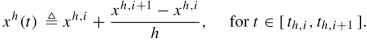
• The state trajectory x^h(t) is obtained by piecewise linear interpolation joining consecutive iterates; specifically, for i = 0, 1, ⋯ , N_h − 1,

  

• The algebraic trajectories y^h(t) and v^h(t) are obtained as piecewise constant functions; specifically, for i = 0, 1, ⋯ , N_h − 1,

  

  It is desirable that these numerical trajectories converge in a sense to be specified, at least subsequentially, to some limiting trajectories that constitute a weak solution of the DVI.

To facilitate the implementation and analysis of the iterations, the discrete-time subproblems need to be defined carefully. For this purpose, we focus on the case where the function F(x, y, v) is given by F(x, y, v) = A(x) + B(x)y + C(x)v; cf. (2.4) for some vector-valued function A and matrix-valued functions B and C. Note the linearity in the pair $u \triangleq (y,v)$ for fixed x. Let x^{h, 0} = x⁰. At time step i ≥ 0, we generate the next iterate (x^{h, i+1}, y^{h, i+1}, v^{h, i+1}) by a backward Euler semi-implicit scheme:

$$\displaystyle \begin{aligned} \begin{array}{cll} x^{h,i+1} & = & x^{h,i} + h \, \left[ \underbrace{A(x^{h,i+1}) + B(x^{h,i})y^{h,i+1} + C(x^{h,i}) v^{h,i+1}}_{\text{note the presence of the unknown iterates}} \, \right] \\[0.3in] 0 \, &\leq& \, y^{h,i+1} \perp G(x^{h,i+1},y^{h,i+1}) \, \geq \, 0 \\ {} v^{h,i+1} & \in & \text{SOL}(K(x^{h,i+1},y^{h,i+1}),H(x^{h,i+1},y^{h,i+1},\bullet)). \end{array} \end{aligned}$$

From the first equation, we may solve for x^{h, i+1} in terms of (x^{h, i}, y^{h, i+1}, u^{h, i+1}) for all h > 0 sufficiently small, provided that ∥A(x)∥ is bounded uniformly for all x. Specifically, we have

$$\displaystyle \begin{aligned} x^{h,i+1} \, = \, \left[ \, \mathbf{I} - h \, A(\bullet) \, \right]^{-1} \left\{ \, x^{h,i} + h \, \left( B(x^{h,i})y^{h,i+1} + C(x^{h,i}) v^{h,i+1} \, \right) \, \right\}. \end{aligned} $$

(2.18)

This solution function may then be substituted into the complementarity and variational conditions, yielding: a quasi-variational inequality (QVI):

where $\widehat {L}^{h,i}(u^{h,i+1}) \triangleq \mathbb {R}^{\ell _1} \times K(x^{h,i+1},y^{h,i+1})$ and

with x^{h, i+1} substituted by the right-hand side in (2.18). Needless to say, the solvability of the latter QVI is key to the well-definedness of the iterations; more importantly, we need to demonstrate that the above QVI has a solution for all h > 0 sufficiently small. Such a demonstration is based on [45, Corollary 2.8.4] specialized to the QVI on hand; namely, with m = ℓ₁ + ℓ₂ where ℓ₁ and ℓ₂ are the dimensions of the vectors y and v, respectively, and with “cl” and “bd” denoting, respectively, the closure and boundary of a set, there exists $\bar {h} > 0$ such that for all $h \in ( 0, \bar {h} ]$,

• $\widehat {L}^{h,i} : \mathbb {R}^m \to \mathbb {R}^m$ is closed-valued and convex-valued;

• there exist a bounded open set $\varOmega \subset \mathbb {R}^m$ and a vector u^{h, i;ref} ∈ Ω such that

• (a) for every $\bar {u} \in \text{cl }\varOmega$, $\widehat {L}^{h,i}(\bar {u}) \neq \emptyset$ and the set limit holds: $\displaystyle {\lim _{u \to \bar {u}}} \widehat {L}^{h,i}(u) = \widehat {L}^{h,i}( \bar {u} )$;

• (b) $z^{h;{\mathrm ref}} \in \widehat {L}^{h,i}(u)$ for every u ∈cl Ω; and

• (c) the set $\left \{ \, u \in \widehat {L}^{h,i}(u) \, \mid \, ( u - u^{h,i;\mathrm {ref}} )^T \widehat {\varPsi }^{h,i}(u) < 0 \, \right \} \, \cap \, \text{bd } \varOmega = \emptyset$.

The above conditions can be shown to hold under the following postulates on the DVI (2.4):

• $A : \mathbb {R}^n \to \mathbb {R}^n$ is continuous and $\displaystyle { \sup _{x \in \mathbb {R}^n} } \, \| \, A(x) \, \| < \infty$;

• $K : \mathbb {R}^n \times \mathbb {R}^{\ell _1}_+ \to \mathbb {R}^{\ell _2}$ is a nonempty-valued, closed-valued, convex-valued, and continuous set-valued map;

• there exists v^ref ∈ K(x, y) for all $(x,y) \in \mathbb {R}^n \times \mathbb {R}^{\ell _1}_+$;

• the map $(y,v) \mapsto \left ( \begin {array}{c} G(x,y) \\ {} H(x,y,v) \end {array} \right )$ is strongly monotone on $\mathbb {R}_+^{\ell _1} \times \mathbb {R}^{\ell _2}$ with a modulus that is independent of $x \in \mathbb {R}^n$.

These postulates are very loose and can be sharpened; they are meant to illustrate the solvability of the subproblems under a set of reasonable assumptions. We will return to discuss more about this issue for the LCS subsequently.

Having constructed the numerical trajectories $\left \{ ( x^h(t),y^h(t),v^h(t) ) \mid h > 0 \right \}$, by piecewise interpolation, we next address the convergence of these trajectories. The result below summarizes the criteria for convergence; for a proof, see [102].

Proposition 3

Suppose that there exist positive constants $\bar {h}$, c_x, and c_u such that for all $h \in ( 0,\bar {h} ]$, and all integers i = 0, 1, ⋯ , N_h − 1,

$$\displaystyle \begin{aligned} \| \, u^{h,i+1} \, \| \, \leq \, c_u \, \left( \, 1 + \| \, x^{h,i} \, \| \, \right) \hspace{1pc} \mathit{\text{and}} \hspace{1pc} \| \, x^{h,i+1} - x^{h,i} \, \| \, \leq \, h \, c_x \, \left( \, 1 + \| \, x^{h,i} \, \| \, \right). \end{aligned}$$

The following two statements hold:

• boundedness: there exist positive constants c _{0 x} , c _{1 x} , c _{0 u} , and c _{1 u} such that for all $h \in ( 0,\bar {h} ]$ ,

  $$\displaystyle \begin{aligned} \displaystyle{ \max_{0 \leq i \leq N_h} } \, \| \, x^{h,i} \, \| \, \leq \, c_{0x} + c_{1x} \, \| \, x^{h,0} \, \| \hspace{1pc} \mathit{\text{and}} \hspace{1pc} \displaystyle{ \max_{1 \leq i \leq N_h} } \, \| \, x^{h,i} \, \| \, \leq \, c_{0u} + c_{1u} \, \| \, x^{h,0} \, \|; \end{aligned}$$

• convergence: there exists a subsequence {h_ν}↓ 0 such that the following two limits exists: $x^{h_{\nu }} \to \widehat {x}^{\, \infty }$ uniformly in $[ 0, \mathscr {T} ]$ and $u^{h_{\nu }} \to \widehat {u}^{\, \infty } = ( \widehat {y}^{\, \infty },\widehat {v}^{\infty } )$ weakly in $L^2(0,\mathscr {T})$ as ν →∞.

The steps in the proof of the above theorem are as follows. Apply the Arzelá-Ascoli Theorem [79, page 57–59] to deduce the uniform convergence of a subsequence $\{ \widehat {x}^{\, h_{\nu }} \}_{\nu \in \kappa }$ to a limit $\widehat {x}^{\, \infty }$ in the supremum, i.e., L^∞-norm:

$$\displaystyle \begin{aligned} \displaystyle{ \lim_{\nu (\in \kappa) \to \infty} } \, \displaystyle{ \sup_{t \in [ 0,\mathscr{T} ]} } \, \| \, \widehat{x}^{h_{\nu}}(t) - \widehat{x}^{\, \infty}(t) \, \| \, = \, 0. \end{aligned}$$

Next, apply Alaoglu’s Theorem [79, page 71–72] to deduce the weak convergence of a further subsequence $\{ \widehat {u}^{\, h_{\nu }} \}_{\nu \in \kappa ^{\, \prime }}$, where κ^′⊆ κ to a limit $\widehat {u}^{\, \infty }$, which implies: for any function $\varphi \in \text{L}^2(0, \mathscr {T})$

$$\displaystyle \begin{aligned} \displaystyle{ \lim_{\nu (\in \kappa^{\, \prime}) \to \infty} } \, \displaystyle{ \int_0^{\, \mathscr{T}} } \, \varphi(s)^T \widehat{u}^{\, h_{\nu^{\, \prime}}}(s) \, ds \, = \, \displaystyle{ \int_0^{\, \mathscr{T}} } \, \varphi(s)^T \widehat{u}^{\, \infty}(s) \, ds. \end{aligned}$$

By Mazur’s Theorem [79, page 88], we deduce the strong convergence of a sequence of convex combinations of $\{ \widehat {u}^{\, h_{\nu }} \}_{\nu \in \kappa ^{\, \prime }}$. A subsequence of such convex combinations converges pointwise to $\widehat {u}^{\, \infty }$ for almost all times in $[ 0, \mathscr {T} ]$; hence by convexity of the graph Gr(K) of the set-valued map K, it follows that $( \widehat {x}^{\, \infty }(t),\widehat {u}^{\infty }(t) ) \in \text{Gr}(K)$ for almost all $t \in [ 0, \mathscr {T} ]$.

Ideally, one would want to establish that every limit tuple $( \widehat {x}^{\infty },\widehat {y}^{\, \infty },\widehat {v}^{\infty } )$ is a weak solution of the DVI (2.4). Nevertheless, the generality of the setting makes this not easy; the case where G(x, y) and H(x, y, v) are separable in their arguments and the set-valued map K is a constant has been analyzed in detail in [102]; the paper [103] analyzed the convergence of a time-stepping method for solving the DVI arising from a frictional contact problem with local compliance. In the next section, we present detailed results for the initial-value LCS (2.3).

2.11 Lecture III: The LCS

Consider the time-invariant, initial-value LCS (2.3):

$$\displaystyle \begin{aligned} \begin{array}{cll} \dot x & = & Ax + Bu, \hspace{1pc} x(0) \, = \, x^0 \\ {} 0 \, &\leq& \, u \perp Cx + Du \, \geq \, 0. \end{array} \end{aligned} $$

(2.19)

For this system, the semi-implicit scheme becomes a (fully) implicit scheme:

$$\displaystyle \begin{aligned} \begin{array}{lll} x^{h,i+1} & = & x^{h,i} + h \, \left( \, Ax^{h,i+1} + Bu^{h,i+1} \, \right), \hspace{1pc} i \, = \, 0, 1, \cdots, N_h - 1 \\ {} 0 \, &\leq& \, u^{h,i+1} \perp Cx^{h,i+1} + Du^{h,i+1} \, \geq \,0 \end{array} \end{aligned}$$

Solving for x^{h, i+1} in the first equation and substituting into the complementarity condition yields the LCP:

$$\displaystyle \begin{aligned} 0 \, \leq \, u^{h,i+1} \, \perp \, q^{h,i+1} + D^{\, h} u^{h,i+1} \, \geq \, 0, \end{aligned} $$

(2.20)

where properties of the matrix $D^{\, h} \triangleq D - C \left [ \, \mathbf {I} - h A \, \right ]^{-1}B$ are central to the well-definedness and convergence of the scheme. The first thing to point out regarding the convergence of the numerical trajectories $( \widehat {x}^{\, h},\widehat {u}^{\, h} )$ is that the matrix D is required to be positive semidefinite, albeit not necessarily definite.

We make several remarks regarding the above iterative algorithm. In general, the iteration matrix D^h is not necessarily positive semidefinite in spite of the same property of D. If the LCP (2.20) has multiple solutions, to ensure the boundedness of at least one such solution, use the least-norm solution obtained from:

boundedness means ∥u^{h, i}∥≤ ρ (1 + ∥x^{h, i}∥) for some constant ρ > 0. In general, the above LCP-constrained least-norm problem is a quadratic program with linear complementarity constraints [16, 17]. When D^h is positive semidefinite as in the case of a “passive” LCS (see definition below), such a least-norm solution can be obtained by an iterative procedure that solves a sequence of linear complementarity subproblems. The same matrix D^h appears in each time step i = 0, 1, ⋯ , N_h − 1; thus some kind of warm-start algorithm can be exploited in practical implementation, if possible, for an initial-value problem. Nevertheless, as with all time-stepping algorithms, the stepwise procedure is not applicable for two-point boundary problems such as (instead of x(0) = x⁰) $Mx(0) + Nx( \mathscr {T} ) = b$, which couples all the iterates $\left \{ x(0) \triangleq x^{h,0}, x^{h,1}, \cdots , x^{h,N_h} \triangleq x( \mathscr {T} ) \right \}$.

In order to present a general convergence result, we need to summarize some key LCP concepts that are drawn from [38]. Given a real square matrix M, the LCP-Range of M, denoted LCP-Range(M), is the set of all vectors q for which the LCP(q, M) is solvable, i.e., SOL(q, M) ≠ ∅; the LCP-Kernel of M, which we denote LCP-Kernel(M), is the solution set SOL(0, M) of the homogeneous LCP: 0 ≤ v ⊥ Mv ≥ 0. An R₀-matrix is a matrix M for which LCP-Kernel(M) = {0}. For a given pair of matrices $A \in \mathbb {R}^{n \times n}$ and $C \in \mathbb {R}^{m \times n}$, let $\overline {\mathscr O}(C,A)$ denote the unobservability space of the pair of matrices (C, A); i.e., $v \in \overline {\mathscr O}(C,A)$ if and only if CAⁱv = 0 for all i = 0, 1, ⋯ , n − 1. The result below employs these concepts; a proof can be found in [57].

Theorem 3

Suppose the following assumptions hold:

• (A) D is positive semidefinite,

• (B) Range(C) ⊆LCP-Range(D^h) for all h > 0 sufficiently small, and

• (C) the implication below holds:

$$\displaystyle \begin{aligned} \begin{array}{r} \left. \begin{array}{r} \mathit{\text{LCP-Kernel}}(D) \ni u^{\infty} \, \perp \, s^{\infty} + CBu^{\infty} \in \left[ \mathit{\text{ LCP-Kernel}}(D) \right]^* \\ {} \mathit{\text{for some }} s^{\infty} \, \in \, \mathit{\text{LCP-Range}}(D) \end{array} \right\} \\[0.2in] \hspace{0.2in} \Rightarrow \ Bu^{\infty} \in \overline{\mathscr O}(C_{\beta \bullet},A), \hspace{1pc} \mathit{\text{where }} {\beta \equiv \{ i : ( Du^{\infty})_i = 0 \}}. \end{array} \end{aligned} $$

(2.21)

Then there exist an $\bar h > 0$ such that, for every x⁰ satisfying Cx⁰ ∈LCP-Range(D), the two trajectories $\widehat x^h(t)$ and $\widehat u^h(t)$ generated by the least-norm time-stepping scheme are well defined for all $h\in (0,\bar h]$ and there is a sequence {h_ν}↓ 0 such that the following two limits exist: $\widehat x^{h_{\nu }}(\cdot ) \rightarrow \widehat x(\cdot )$ uniformly on $[ 0,\mathscr {T}]$ and $\widehat u^{h_{\nu }}(\cdot ) \rightarrow \widehat u(\cdot )$ weakly in L²(0, T). Moreover, all such limits $(\widehat x(\cdot ), \widehat u(\cdot ))$ are weak solutions of the initial-value LCS (2.19).

A large class of LCSs that satisfy the assumptions of the above theorem is of passive type [28, 34]. A linear system Σ(A, B, C, D) given by

$$\displaystyle \begin{aligned} \begin{array}{rcl} \dot x(t) & = & Ax(t) + Bz(t) \\ {} w(t) & = & Cx(t)+Dz(t) \end{array} \end{aligned} $$

(2.22)

is passive if there exits a nonnegative-valued function $V: \mathbb {R}^n \rightarrow \mathbb {R}_+$ such that for all t₀ ≤ t₁ and all trajectories (z, x, w) satisfying the system (2.22), the following inequality holds:

$$\displaystyle \begin{aligned}V(x(t_0))+\int_{t_0}^{t_1}z^T(t)w(t)dt \geq V(x(t_1)).\end{aligned}$$

Passivity is a fundamental property in linear systems theory; see the two cited references. Moreover, it is well known that the system Σ(A, B, C, D) is passive if and only if there exists a symmetric positive semidefinite matrix K such that the following symmetric matrix:

$$\displaystyle \begin{aligned} \left[ \begin{array}{cc} A^TK+KA & KB-C^T \\ {} B^TK-C & -(D+D^T) \end{array} \right] \end{aligned} $$

(2.23)

is negative semidefinite. Checking passivity can be accomplished by solving a linear matrix inequality using methods of semidefinite programming [19].

Corollary 1

If Σ(A, B, C, D) is passive, then the conclusion of Theorem 3 holds.

2.12 Lecture III: Boundary-Value Problems

A classic family of methods for solving boundary-value ODEs [11, 12, 72] (see also [132, Section 7.3]) is that of shooting methods. The basic idea behind these methods is to cast the boundary-value problem as a system of algebraic equations whose unknown is the initial condition that defines an initial-value ODE. An iterative method, such as a bisection or Newton method, for solving the algebraic equations is then applied; each evaluation of the function defining the algebraic equations requires solving an initial-value ODE. Multiple-shooting methods refine this basic idea by first partitioning the time interval of the problem into smaller sub-intervals on each of which a boundary-value problem is solved sequentially. Convergence of the overall method requires differentiability of the algebraic equations if a Newton-type method is employed to facilitate speed-up. In what follows, we apply the basic idea of a shooting method to the time-invariant, boundary-value DVI:

$$\displaystyle \begin{aligned} \begin{array}{clll} \dot x & = & F(x,u) \\ {} u & \in & \text{SOL}\left( K,H(x,\bullet) \right) \\ {} 0 & = & \varPsi(x(0),x( \mathscr{T} )). \end{array} \end{aligned} $$

(2.24)

For simplicity, suppose that the mapping H(x, •) is strongly monotone with a modulus independent of x. This implies for every x⁰, the ODE $\dot {x} = F(x,u(x))$ with x(0) = x⁰, where u(x) is the unique solution of the VI (K, H(x, •)), has a unique solution which we denote x(t;x⁰). This solution determines the terminal condition $x( \mathscr {T} )$ uniquely as $x(\mathscr {T};x^0)$. Thus the two-point boundary-value problem becomes the algebraic equation:

(2.25)

As a function of its argument, Φ is typically not differentiable; thus a fast method such as the classical Newton method is not applicable. Nevertheless, a “semismooth Newton method” [45, Chapter 7] can be applied provided that Φ is a semismooth function. In turn, this will be so if for instance the boundary function Ψ is differentiable and the solution $x(\mathscr {T};\bullet )$ depends semismoothly on the initial condition x⁰. In what follows, we present the semismoothness concept [106] and the resulting Newton method for finding a root of Φ, which constitutes the basic shooting method for solving the boundary-value DVI (2.24). We warn the reader that this approach has not been tested in practice and refinements are surely needed for the method to be effective.

There are several equivalent definitions of semismoothness. The following one based on the directional derivative is probably the most elementary without requiring advanced concepts in nonsmooth analysis.

Definition 1

Let $G : \varOmega \subseteq \Re ^n \to \Re ^m$, with Ω open, be a locally Lipschitz continuous function on Ω. We say that G is semismooth at a point $\bar x\in \varOmega$ if G is directionally differentiable (thus B(ouligand)-differentiable) near $\bar x$ and such that

$$\displaystyle \begin{aligned} \displaystyle{ \lim_{\bar{x} \neq x \to \bar{x}} } \, \displaystyle{ \frac{\|\, G^{\, \prime}(x;x-\bar x) - G^{\, \prime}(\bar{x};x-\bar x)\,\|}{ \|\, x-\bar x\,\|} } \, = \, 0. \end{aligned} $$

(2.26)

If the above requirement is strengthened to

$$\displaystyle \begin{aligned} \limsup_{\bar{x} \neq x \to \bar{x}} \, \frac{\| \, G^{\, \prime}(x;x-\bar x)- G^{\, \prime}(\bar{x};x-\bar x)\,\|}{ \|\, x-\bar x\,\|{}^2} \, < \, \infty, \end{aligned} $$

(2.27)

we say that G is strongly semismooth at $\bar {x}$. If G is (strongly) semismooth at each point of Ω, then we say that G is (strongly) semismooth on Ω.

Let $\varXi _{\mathscr {T}} \triangleq \{ x(t,\xi ^0) \mid t \in [ 0,\mathscr {T} ] \}$, where x(t, ξ) is a solution of the ODE with initial condition: $\dot {x} = f(x)$ and x(0) = ξ⁰. Suppose that f is Lipschitz continuous and directionally differentiable, thus B(ouligand)-differentiable, in an open neighborhood $\mathscr {N}_T$ containing $\varXi _{\mathscr {T}}$. The following two statements hold:

• x(t, •) is B-differentiable at ξ⁰ for all $t \in [ 0,\mathscr {T} ]$ with the directional derivative x(t, •)^′(ξ⁰;η) being the unique solution y(t) of the directional ODE:

  $$\displaystyle \begin{aligned} \dot{y}(t) \, = \, f^{\, \prime}(x(t,\xi^0);y); \hspace{1pc} y(0) \, = \, \eta; \end{aligned} $$

  (2.28)

• if f is semismooth at all points in $\mathscr {N}_{\mathscr {T}}$, then x(t, •) is semismooth at ξ⁰ for all $t \in [ 0,\mathscr {T} ]$.

Before introducing the semismooth-based shooting method, we need to address the question of when the solution u(x) of the VI (K, H(x, •)) is a semismooth function of x. A broad class of parametric VIs that possess this property is when K is a polyhedron, or more generally, a finitely representable convex set satisfying the constant rank constraint qualification (CRCQ) [45, Chapter 4]. For simplicity, we present the results for the case where K is a polyhedron. Suppose that u^∗ is a strongly regular solution of the VI (K, H(x^∗, •)). Similar to the NCP, there exist open neighborhoods $\mathscr {V}$ and $\mathscr {U}$ of x^∗ and u^∗, respectively, and a B-differentiable function $u : \mathscr {V} \to \mathscr {U}$ such that for every $x \in \mathscr {V}$, u(x) is the unique solution in $\mathscr {U}$ that is a solution of the VI (K, H(x, •)); moreover, the directional derivative u^′(x^∗;dx) at x^∗ along a direction dx is given as the unique solution du of the CP:

$$\displaystyle \begin{aligned} \begin{array}{rll} du & \in & \underbrace{\mathscr{T}(K;x^*) \, \cap \, H(x^*,u^*)^{\perp}}_{\text{critical cone } {\mathscr{C}(x^*)}} \\[0.2in] J_x H(x^*,u^*) dx + J_u H(x^*,u^*) du & \in & \left[ \, \mathscr{T}(K;x^*) \, \cap \, H(x^*,u^*)^{\perp} \, \right]^* \\ {} du & \perp & J_x H(x^*,u^*) dx + J_u H(x^*,u^*) du, \end{array} \end{aligned} $$

(2.29)

where $\mathscr {T}(K;x^*)$ is the tangent cone of K at x^∗ and H(x^∗, u^∗)^⊥ denotes the orthogonal complement of the vector H(x^∗, u^∗).

Returning to the DVI (2.24), we may deduce that, assuming the differentiability of F and H, the strong regularity of the solution u(x(t, ξ⁰)) of the VI (K, H(x(t, ξ⁰), •)), and by combining (2.28) with (2.29), x(t, •)^′(ξ⁰;η) is the unique solution y(t) of:

$$\displaystyle \begin{aligned} \begin{array}{l} \dot{y}(t) \, = \, J_xF(x(t,\xi^0),u(x(t,\xi^0))) y + J_uF(x(t,\xi^0),u(x(t,\xi^0)))v, \ \\[0.15in] y(0) \, = \, \eta v \, \in \, \mathscr{C}(x(t,\xi^0)) \\ {} J_xH(x(t,\xi^0),u(x(t,\xi^0)))y + J_uH(x(t,\xi^0),u(x(t,\xi^0)))v \, \in \, \left[ \, \mathscr{C}(x(t,\xi^0)) \, \right]^* \\ {} v \, \perp \, J_xH(x(t,\xi^0),u(x(t,\xi^0)))y + J_uH(x(t,\xi^0),u(x(t,\xi^0)))v, \end{array} \end{aligned}$$

or equivalently,

$$\displaystyle \begin{aligned} \begin{array}{rll} \dot{x} & = & F(x,u), \hspace{1pc} x(0) \, = \, \xi^0 \\ {} \dot{y} & = & J_xF(x,u) y + J_uF(x,u) v, \hspace{1pc} y(0) \, = \, \eta \\ {} u & \in & \text{SOL}(K,H(x,\bullet)) \\ {} \mathscr{C}(x) \, &\ni& \, v \perp J_xH(x,u) y + J_uH(x,u)v \, \in \, \left[ \, \mathscr{C}(x(t)) \, \right]^*. \end{array} \end{aligned}$$

Let

we deduce that the triple (x(t, ξ⁰), u(x(t, ξ⁰)), x(t, •)^′(ξ⁰;η)) is the unique triplet (x, u, y), which together with an auxiliary variable z, satisfies the DVI:

$$\displaystyle \begin{aligned} \begin{array}{lll} \dot{z} & = & \widehat{F}(z,w); \hspace{1pc} z(0) \, = \, ( \xi^0,\eta ) \\ {} w & \in & \text{SOL}(\widehat{K}(z),\widehat{H}). \end{array} \end{aligned}$$

This is a further instance of a DVI where the defining set of the variational condition varies with the state variable; cf. (2.4).

Returning to the algebraic equation reformulation (2.25) of the boundary-value DVI (2.4), we sketch the semismooth Newton method for finding a zero x⁰ of the composite function $\varPhi (x^0) = \varPsi (x^0,x(\mathscr {T},x^0))$. This is an iterative method wherein at each iteration ν, given a candidate zero ξ^ν, we compute a generalized Jacobian matrix A(ξ^ν) of Φ at ξ^ν and then let the next iterate x^ν+1 be the (unique) solution of the (algebraic) linear equation: Φ(ξ^ν) + A(ξ^ν)(ξ − ξ⁰) = 0. This is the version of the method where a constant unit step size is employed. Under a suitable nonsingularity assumption at an isolated zero of Φ whose semismoothness is assumed, local superlinear convergence of the generated sequence of (vector) iterates can be proved; see [45, Chapter 7]. To complete the description of the method, the matrix A(ξ^ν) needs to be specified. As a composite function of Ψ and the solution function $x(\mathscr {T},\bullet )$, A(ξ^ν) can be obtained by the chain rule provided that a generalized Jacobian matrix of the latter function at the current iterate ξ^ν is available. Details of this can be found in [100] which also contains a statement of convergence of the overall method.

2.13 Lecture III: Summary

In this lecture, we have

• introduced a basic numerical time-stepping method for solving the DVI (2.4),

• provided sufficient conditions for the weak, subsequential convergence of the method,

• specialized the method to the LCS and presented sharpened convergence results, including the case of a passive system, and

• outlined a semismooth Newton method for solving an algebraic equation reformulation of a boundary-value problem, whose practical implementation requires further study.

2.14 Lecture IV: Linear-Quadratic Optimal Control Problems

An optimal control problem is the building block of a multi-agent optimization problem in continuous time. In this lecture, we discuss the linear-quadratic (LQ) case of the (single-agent) optimal control problem in preparation for the exposition of the multi-agent problem in the next lecture. The LQ optimal control problem with mixed state-control constraints is to find continuous-time trajectories $(x,u) : [ 0,\mathscr {T} ] \to \mathbb {R}^{n+m}$ to

(2.30)

where the matrices $\varXi \triangleq \left [ \begin {array}{cc} P & Q \\ {} Q^{\, T} & R \end {array} \right ]$ and S are symmetric positive semidefinite. Unlike these time-invariant matrices and the constant vector f, (p;q;r) is a triple of properly dimensioned Lipschitz continuous vector functions. The semi-coercivity assumption on the objective function, as opposed to coercivity, is a major departure of this setting from the voluminous literature on this problem. For one thing, the existence of an optimal solution is no longer a trivial matter. Ideally, we should aim at deriving an analog of Proposition 4 below for a convex quadratic program in finite dimensions, which we denote QP(Z(b), e, M):

where M is an m × m symmetric positive semidefinite matrix, $Z(b) \triangleq \{ z \in \mathbb {R}^m \mid Ez + b \geq 0 \}$, where E is a given matrix and e and b are given vectors, all of appropriate orders. It is well known that the polyhedron Z(b) has the same recession cone $Z_{\infty } \triangleq \{ v \in \mathbb {R}^m \mid Ev \geq 0 \}$ for all b for which Z(b) ≠ ∅. Let SOL(Z(b), e, M) denote the optimal solution set of the above QP.

Proposition 4

Let M be symmetric positive semidefinite and let E be given. The following three statements hold.

• (a) For any vector b for which Z(b) ≠ ∅, a necessary and sufficient condition for the QP(Z(b), e, M) to have an optimal solution is that e^Td ≥ 0 for all d in Z_∞∩ker(M).

• (b) If Z_∞∩ker(M) = {0}, then SOL(Z(b), e, M) ≠ ∅ for all (e, b) for which Z(b) ≠ ∅.

• (c) If SOL(Z(b), e, M) ≠ ∅, then $\mathit{\text{SOL}}(Z(b),e,M) = \{ z \in Z(b) \mid Mz = M\widehat {z}, \, e^T \widehat {z} = e^T \widehat {z} \}$ for any optimal solution $\widehat {z}$; thus MSOL(Z(b), e, M) is a singleton whenever it is nonempty.

Extending the KKT conditions for the QP(Z(b), e, M):

$$\displaystyle \begin{aligned} \begin{array}{lll} 0 & = & e + Mz - E^T\mu \\ {} 0 & \leq & \mu \, \perp \, Ez + b \, \geq \, 0, \end{array} \end{aligned}$$

we can derive a 2-point BV-LCS formulation of (2.30) as follows. We start by defining the Hamiltonian function:

where λ is the costate (also called adjoint) variable of the ODE $\dot {x}(t) = Ax(t) + Bu(t) + r$, and the Lagrangian function:

where μ is the Lagrange multiplier of the algebraic constraint: Cx + Du + f ≥ 0. Inspired by the Pontryagin Principle [139, Section 6.2] and [61, 112], we introduce the following DAVI:

$$\displaystyle \begin{aligned} \left( \begin{array}{c} \dot{\lambda}(t) \\ {} \dot{x}(t) \end{array} \right) \, = \, \left( \begin{array}{c} -p(t) \\ {} r(t) \end{array} \right) + \left[ \begin{array}{cc} -A^T & -P \\ {} 0 & A \end{array} \right] \left( \begin{array}{c} \lambda(t) \\ {} x(t) \end{array} \right) + \left[ \begin{array}{c} -Q \\ {} B \end{array} \right] u(t) + \left[ \begin{array}{c} C^{\, T} \\ {} 0 \end{array} \right] \mu(t) \end{aligned}$$

(2.31)

where $U(x) \triangleq \{ u \in \mathbb {R}^m \mid Cx + Du + f \geq 0 \}$. Note that the above is a DAVI with a boundary condition: λ(T) = c + Sx(T); this is one challenge of this system. Another challenge is due to the mixed state-control constraint: Cx(t) + Du(t) + f ≥ 0. While the membership implies the existence of a multiplier $\widehat {\mu }(t)$ such that

$$\displaystyle \begin{aligned} \begin{array}{l} 0 \, = \, q(t) + Q^Tx(t) + Ru(t) + B^T\lambda(t) - D^T \widehat{\mu}(t) \\ {} 0 \, \leq \, \widehat{\mu}(t) \, \perp \, Cx(t) + Du(t) + f \, \geq \, 0, \end{array} \end{aligned}$$

we seek in (2.31) a particular multiplier μ(t) that also satisfies the ODE. So far, we have only formally written down the formulation (2.31) without connecting it to the optimal control problem (2.30). As a DAVI with (x, λ) as the pair of differential variables and (u, μ) as the pair of algebraic variables, the tuple (x, u, λ, μ) is a weak solution of (2.31) if (i) (x, λ) is absolutely continuous and (u, μ) is integrable on $[ 0, \mathscr {T} ]$, (ii) the differential equation and the two algebraic conditions hold for almost all $t \in ( 0,\mathscr {T} )$, and (iii) the initial and boundary conditions are satisfied.

In addition to the positive semidefiniteness assumption of the matrices Ξ and S, we need three more blanket conditions assumed to hold throughout the following discussion:

• (a feasibility assumption) a continuously differentiable function $\widehat {x}_{\mathrm {fs}}$ with $\widehat {x}_{\mathrm {fs}}(0) = \xi$ and a continuous function $\widehat {u}_{\mathrm {fs}}$ exist such that for all t ∈ [0, T]: $d \widehat {x}_{\mathrm {fs}}(t)/dt \, = \, A\widehat {x}_{\mathrm {fs}}(t) + B\widehat {u}_{\mathrm {fs}}(t) + r(t)$ and $\widehat {u}_{\mathrm {fs}}(t) \, \in \, U( \widehat {x}_{\mathrm {fs}}(t))$;

• (a primal condition) [Ru = 0, Du ≥ 0] implies u = 0;

• (a dual condition) [D^Tμ = 0, μ ≥ 0] implies (CAⁱB)^Tμ = 0 for all integers i = 0, ⋯ , n − 1, or equivalently, for all nonnegative integers i.

It is easy to see that the primal Slater condition: [$\exists \, \widehat {u}$ such that $D\widehat {u} > 0$] implies the dual condition, but not conversely. For more discussion of the above conditions, particularly the last one, see [59].

Here is a roadmap of the main Theorem 4 below. It starts with the above postulates, under which part (I) asserts the existence of a weak solution of the DAVI (2.31) in the sense of Carathéodory. The proof of part (I) is based on a constructive numerical method. Part (II) of Theorem 4 asserts that any weak solution of the DAVI yields an optimal solution of (2.30); this establishes the sufficiency of the Pontryagin optimality principle. The proof of this part is based on a direct verification of the assertion, from which we can immediately obtain several properties characterizing an optimal solution of (2.30). These properties are summarized in part (III) of the theorem. From these properties, part (IV) shows that any optimal solution of (2.30) must be a weak solution of the DAVI (2.31), thereby establishing the necessity of the Pontryagin optimality principle. Finally, part (V) asserts the uniqueness of the solution obtained from part (I) under the positive definiteness of the matrix R.

Theorem 4

Under the above setting and assumptions, the following five statements (I–V) hold.

(I: Solvability of the DAVI) The DAVI (2.31) has a weak solution (x^∗, λ^∗, u^∗, μ^∗).

(II: Sufficiency of Pontryagin) If (x^∗, λ^∗, u^∗, μ^∗) is any weak solution of (2.31), then the pair (x^∗, u^∗) is an optimal solution of the problem (2.30).

(III: Gradient characterization of optimal solutions) If $( \widehat {x},\widehat {u} )$ and $( \widetilde {x},\widetilde {u} )$ are any two optimal solutions of (2.30), then the following three properties hold:

• (a) for almost all t ∈ [0, T],

  $$\displaystyle \begin{aligned} \left[ \begin{array}{cc} P & Q \\ {} Q^T & R \end{array} \right] \left( \begin{array}{c} \widehat{x}(t) - \widetilde{x}(t) \\ {} \widehat{u}(t) - \widetilde{u}(t) \end{array} \right) \, = \, 0, \end{aligned}$$

• (b) $S \widehat {x}(T) = S \widetilde {x}(T)$ , and

• (c) $c^T ( \widehat {x}(T) - \widetilde {x}(T) ) + \displaystyle { \int _0^{\, T} } \, \left ( \begin {array}{c} p(t) \\ {} q(t) \end {array} \right )^T \left ( \begin {array}{c} \widehat {x}(t) - \widetilde {x}(t) \\ {} \widehat {u}(t) - \widetilde {u}(t) \end {array} \right ) \, dt \, = \, 0$.

Thus given any optimal solution $( \widehat {x},\widehat {u} )$ of (2.30), a feasible tuple $( \widetilde {x},\widetilde {u} )$ of (2.30) is optimal if and only if conditions (a), (b), and (c) hold.

(IV: Necessity of Pontryagin) Let (x^∗, λ^∗, u^∗, μ^∗) be the tuple obtained from part (I). A feasible tuple $( \widetilde {x},\widetilde {u} )$ of (2.30) is optimal if and only if $(\widetilde {x},\lambda ^*,\widetilde {u},\mu ^*)$ is a weak solution of (2.31).

(V: Uniqueness under positive definiteness) If R is positive definite, then for any two optimal solutions $( \widehat {x},\widehat {u} )$ and $( \widetilde {x},\widetilde {u} )$ of (2.30), $\widehat {x} = \widetilde {x}$ everywhere on [0, T] and $\widehat {u} = \widetilde {u}$ almost everywhere on [0, T]. In this case (2.30) has a unique optimal solution $( \, \widehat {x},\widehat {u} \, )$ such that $\widehat {x}$ is continuously differentiable and $\widehat {u}$ is continuous on [0, T], and for any optimal $\widehat {\lambda }$, for all t ∈ [0, T].

It should be noted that in part (V) of the above, the uniqueness requires the positive definiteness of the principal block R of Ξ, and not of this entire matrix Ξ, which nonetheless is assumed to be positive semidefinite. The reason is twofold: one: via the ODE, the state variable x can be solved uniquely in terms of the control variable u; two: part (I) implies that the difference $\widehat {u} - \widetilde {u}$ is equal to $R^{-1}Q \widehat {x} - \widetilde {x}$ for any two solution pairs $( \widetilde {x},\widetilde {u} )$ and $( \widetilde {x},\widetilde {u} )$. Combining these two consequences yields the uniqueness in part (V) under the positive definiteness assumption of R. This is the common case treated in the optimal control literature.

2.14.1 The Time-Discretized Subproblems

A general time-stepping method for solving the LQ problem (2.30) proceeds similarly to (2.16), albeith with suitable modifications as described below. Let h > 0 be an arbitrary step size such that $N_h \triangleq \displaystyle { \frac {T}{h} }$ is a positive integer. We partition the interval $[ 0, \mathscr {T} ]$ into N_h subintervals each of equal length h:

Thus t_h,i+1 = t_h,i + h for all i = 0, 1, ⋯ , N_h − 1. We step forward in time and calculate the state iterates ${\mathbf {x}}^h \triangleq \left \{ x^{h,i} \right \}_{i=0}^{N_h}$ and control iterates ${\mathbf {u}}^h \triangleq \left \{ u^{h,i} \right \}_{i=1}^{N_h}$ by solving N_h finite-dimensional convex quadratic subprograms, provided that the latter are feasible. From these discrete-time iterates, continuous-time numerical trajectories are constructed by piecewise linear and piecewise constant interpolation, respectively. Specifically, define the functions $\widehat {x}^{\, h}$ and $\widehat {u}^{\, h}$ on the interval [0, T]: for all i = 0, ⋯ , N_h − 1:

(2.32)

The convergence of these trajectories as the step size h ↓ 0 to an optimal solution of the LQ control problem (2.30) is a main concern in the subsequent analysis. Neverthless, since the DAVI (2.31) is essentially a boundary-value problem, care is needed to define the discretized subproblems so that the iterates (x^h, u^h) are well defined. Furthermore, since the original problem (2.30) is an infinite-dimensional quadratic program, one would like the subproblems to be finite-dimensional QPs. The multipliers of the constraints in the latter QPs will then define the adjoint trajectory $\widehat {\lambda }^{\, h}(t)$ and the algebraic trajectory $\widehat {\mu }^{\, h}(t)$; see below.

In an attempt to provide a common framework for the analysis of the backward Euler discretization and the model predictive control scheme [48, 50, 92] that has a long tradition in optimal control problems, a unified discretization method was proposed in [59] that employed several families of matrices {B(h)}, {A(h)}, {E(h)} and $\{ \widehat {E}(h) \}$ parametrized by the step h > 0; these matrices satisfy the following limit properties:

$$\displaystyle \begin{aligned} \displaystyle{ \lim_{h \downarrow 0} } \, \displaystyle{ \frac{A(h) - I}{h} } \, = \, A; \hspace{1pc} \displaystyle{ \lim_{h \downarrow 0} } \, \displaystyle{ \frac{B(h)}{h} } \, = \, B; \hspace{1pc} \text{and} \hspace{1pc} \displaystyle{ \lim_{h \downarrow 0} } \, \displaystyle{ \frac{E(h)}{h} } \, = \, \displaystyle{ \lim_{h \downarrow 0} } \, \displaystyle{ \frac{\widehat{E}(h)}{h} } \, = \, I.\end{aligned} $$

Furthermore, in order to ensure that each discretized subproblem is solvable, a two-step procedure was introduced: the first step computes the least residual of feasibility of such a subproblem by solving the linear program:

(2.33)

$$\displaystyle \begin{aligned} \left\{ \begin{array}{l} x^{h,i+1} \, = \, \left[ \, \theta \, E(h) \, r^{h,i}+ ( 1-\theta ) \, \widehat{E}(h) \, r^{h,i+1} \, \right] + A(h)x^{h,i}+B(h)u^{h,i+1} \\ {} Cx^{h,i+1} + Du^{h,i+1} + f + \rho \, \mathbf{1} \, \geq \, 0 \end{array} \right\},\end{aligned} $$

where $r^{h,i} \triangleq r(t_{h,i})$ for all i = 0, 1, ⋯ , N_h, and 1 is the vector of all ones. The above linear program must have a finite optimal solution and the optimal objective value ρ_h(ξ) satisfies lim_h↓0 ρ_h(ξ)  =  0; this limit ensures that the pair of limit trajectories $\widehat {x}^{\, h}(t)$ and $\widehat {u}^{\, h}(t)$ constructed from the discrete-time iterates will be feasible to (2.30) for almost all times $t \in [ 0, \mathscr {T} ]$. The scalar θ ∈ [0, 1] adds flexibility to the above formulation and leads to different specific schemes with proper choices. For instance, when θ = 0, by letting $\widehat {E}(h) \triangleq h A(h)$, $A(h) \triangleq (I-hA)^{-1}$, and $B(h) \triangleq h A(h)B$, we obtain a standard backward Euler discretization of the ODE constraint in (2.30). When θ = 1, by letting $E(h) \triangleq \displaystyle {\int _{0}^h e^{As}ds}$, $A(h) \triangleq e^{Ah}$, and $B(h) \triangleq \displaystyle {\int _0^h e^{As}ds} B$, we obtain the MPC approximation of this ODE.

Employing the minimum residual ρ_h(ξ), the relaxed, unified time-stepping method solves the following (feasible) convex quadratic program at time t_h,i+1:

$$\displaystyle \begin{aligned} \left\{ \begin{array}{l} x^{h,i+1} \, = \, \left[ \, \theta \, E(h) \, r^{h,i}+ ( 1-\theta ) \, \widehat{E}(h) \, r^{h,i+1} \, \right] + A(h)x^{h,i}+B(h)u^{h,i+1} \\ {} f + Cx^{h,i+1} + Du^{h,i+1} + \underbrace{\rho_h(\xi) \, \mathbf{1}}_{\text{relaxed feasibility}} \, \geq \, 0 \end{array} \right\} . \end{aligned}$$

The primal condition on the pair (R, D) and the use of the least residual ρ_h(ξ) are sufficient to ensure that an optimal solution to the above QP exists. Notice that unlike the case in Lecture III of an initial-value DVI (2.16) or the LCS (2.19), the $\widehat {\text{QP}}^{\, h}$ is coupled in the discrete-time iterates and does not decompose into individual subproblems according to the time steps. Thus this quadratic subprogram is potentially of very large size and its practical solution requires care.

Letting $\{ \lambda ^{h,i} \}_{i=0}^{N_h}$ be the multipliers of the discrete-time state constraints and $\{ \mu ^{h,i+1} \}_{i=0}^{N_h}$ be the multipliers of the algebraic state-control inequalities, we define the λ-trajectory similarly to the x-trajectory; namely, for i = 0, ⋯ , N_h,

with $\lambda ^{h,N_h+1} \triangleq c + Sx^{h,N_h+1}$, and the μ-trajectory similarly to the u-trajectory; namely, for i = 0, ⋯ , N_h,

The convergence of the numerical trajectories is formally stated in the theorem below.

Theorem 5

Assume the setting state above. Let $\widehat {x}^h(t)$ and $\widehat {u}^h(t)$ be as defined by (2.32) and $\widehat {\lambda }^{\, h}(t)$ and $\widehat {\mu }^{\, h}(t)$ as above. The following four statements hold.

• (a) There exists a sequence of step sizes {h_ν}↓ 0 such that the two limits exist: $\left ( \, \widehat x^{\, h_{\nu }}, \widehat {\lambda }^{\, h_{\nu }} \, \right ) \rightarrow \left ( \, \widehat {x}, \widehat {\lambda } \, \right )$ uniformly on [0, T] and $\left ( \, \widehat u^{\, h_{\nu }}, \widehat {\mu }^{\, h_{\nu }} \, \right ) \rightarrow \left ( \widehat u, \widehat {\mu } \right )$ weakly in L²(0, T); moreover, $\widehat {x}$ and $\widehat {\lambda }$ are Lipschitz continuous.

• (b) The sequences $\left \{ \displaystyle { \left [ \begin {array}{cc} P & Q \\ Q^T & R \end {array} \right ] \left ( \begin {array}{c} \widehat {x}^{\, h} \\ \widehat {u}^{\, h} \end {array} \right ) } \right \}$ and $\left \{ D^T \widehat {\mu }^{\, h} \right \}$ converge to $\displaystyle { \left [ \begin {array}{cc} P & Q \\ Q^T & R \end {array} \right ] }\left ( \begin {array}{c} \widehat {x} \\ \widehat {u} \end {array} \right )$ and $D^T \widehat {\mu }$ uniformly on [0, T], respectively.

• (c) Any limit tuple $( \widehat x, \widehat u, \widehat {\lambda }, \widehat \mu )$ from (a) is a weak solution of (2.31); thus $( \widehat {x}, \widehat {u} )$ is an optimal solution of (2.30).

• (d) Part (I) of Theorem 4 holds.

The proof of the above theorem hinges on establishing the bounds in Proposition 3 for the differential iterates (x^{h, i}, λ^{h, i}) and the algebraic iterates (u^{h, i}, μ^{h, i}). This is highly technical, partly due the relaxed assumptions we have made—e.g., the positive semidefiniteness, instead of positive definiteness of the matrix $\varXi \triangleq \left [ \begin {array}{cc} P & Q \\ {} Q^{\, T} & R \end {array} \right ]$—and partly due to the boundary-value nature of the DAVI. Details can be found in [59].

When R is positive definite, we can establish the uniform convergence of the u-variable by redefining the discrete-time trajectory $\widehat {u}^{\, h}$ using piecewise linear interpolation instead of the piecewise constant interpolation in the semidefinite case. First notice that u^{h, 0} is not included in the ($\widehat {\text{QP}}^{\, h}$). By letting u^{h, 0} be the unique solution of the QP at the initial time t = 0,

we redefine

(2.34)

It can be shown that the sequences of state and control trajectories $\{ \widehat {x}^{\, h} \}$ and $\{ \widehat {u}^{\, h} \}$ converge, respectively, to the unique optimal solution $( \widehat {x},\widehat {u} )$ of the problem (2.30) with $\widehat {x}$ being continuously differentiable and $\widehat {u}$ Lipschitz continuous on [0, T]. We omit the details.

2.15 Lecture IV: Summary

In this lecture, we have

• introduced the linear-quadratic optimal control problem with mixed state-control constraints

• described a time-stepping method for solving the problem that unifies time stepping and model predictive control, and

• presented a convergence result under a set of assumptions.

This development is the basis for extension to a multi-agent non-cooperative game where each player solves such an LQ optimal control problem parameterized by the rivals’ time-dependent strategies.

2.16 Lecture V: Open-Loop Differential Nash Games

Non-cooperative game theory provides a mathematical framework for conflict resolution among multiple selfish players each seeking to optimize his/her individual objective function that is impacted by the rivals’ decisions and subject to constraints that may be private, coupled, or shared. A solution concept of such a game was introduced by John Nash and has been known as a Nash equilibrium. There have been several recent surveys on the static Nash equilibrium problem defined in terms of multiple finite-dimensional optimization problems, one for each player; see e.g. [44, 46] where the reader can also find an extensive literature including historical account, theory, algorithms, and selected applications. This lecture pertains to the Nash equilibrium problem (NEP) defined in continuous time wherein each player’s optimization problem is the single-agent LQ optimal control problem discussed in the last lecture and extended herein to the case of multiple agents. The discussion below is drawn from the recently published paper [110].

Specifically, we consider a linear-quadratic (LQ) N-player noncooperative game on the time interval $[ 0, \mathscr {T} ]$, where $\mathscr {T} < \infty$ is the finite horizon and N is the number of players of the game. Each player i ∈{1, ⋯ , N} chooses an absolutely continuous state function $x_i : [ 0, \mathscr {T} ] \to \mathbb {R}^{n_i}$ and a bounded measurable (thus integrable) control function $u_i : [ 0,\mathscr {T} ] \to \mathbb {R}^{m_i}$ for some positive integers n_i and m_i via the solution of a LQ optimal control problem. These state and control variables are constrained by a player-specific ODE and a linear inequality system.

Notation

$x_{-i} \triangleq \left ( x_j \right )_{i \neq j=1}^N$; $u_{-i} \triangleq \left ( u_j \right )_{i \neq j=1}^N$ denote the rivals’ pairs of state and control variables, respectively.

Anticipating the pair (x_−i, u_−i) of rivals’ trajectory and treating only private constraints, player i solves

(2.35)

where each W_ii and $\left [ \begin {array}{cc} P_{ii} & Q_{ii} \\ {} R_{ii} & S_{ii} \end {array} \right ]$are symmetric positive semidefinite, resulting in (2.35) being a convex LQ optimal control problem in player i’s variables. The other notations are extensions of (2.30) that is the case of a single player. Moreover, the assumptions previously introduced for (2.30) extend to each player’s problem in the game.

An aggregated pair of trajectories (x^∗, u^∗), where ${\mathbf {x}}^*\, \triangleq \, \left ( x_i^* \right )_{i=1}^N$ and ${\mathbf {u}}^* \,\triangleq \, \left ( u_i^* \right )_{i=1}^N$, is a Nash equilibrium (NE) of the above game if for each i = 1, ⋯ , N,

Toward the analysis of this game, we distinguish two cases:

• $\varXi _{ii^{\, \prime }} \triangleq \left [ \begin {array}{cc} P_{ii^{\, \prime }} & Q_{ii^{\, \prime }} \\ {} R_{ii^{\, \prime }} & S_{ii^{\, \prime }} \end {array} \right ] = \left [ \begin {array}{cc} P_{i^{\, \prime }i} & Q_{i^{\, \prime }i} \\ {} R_{i^{\, \prime }i} & S_{i^{\, \prime }i} \end {array} \right ]^T \triangleq \varXi _{i^{\, \prime } i}^T$ and $W_{ii^{\, \prime }} = W_{i^{\, \prime } i}^T$ for all i ≠ i^′, reflecting the symmetric impact of the strategy of player i^′ on player i’s objective function and vice versa.

• $\left ( W_{i i^{\, \prime }},\varXi _{ii^{\, \prime }} \right ) \neq \left ( W_{i^{\, \prime } i}^T , \varXi _{i^{\, \prime }i}^T \right )$ for some i ≠ i^′, reflecting the asymmetric impact of the strategy of player i^′ on player i’s objective function and vice versa.

The treatment of these two cases is different. In the symmetric case, we show that a NE of the game can be obtained as a stationary solution of a single optimal control problem with an objective function that is the sum of the players’ objectives and whose constraints are the Cartesian product of the individual players’ constraints. In the asymmetric case, we provide a best-response algorithm to constructively establish the existence of a NE to the game; such an algorithm iteratively solves single-player LQ optimal control problems by fixing the rivals’ variables at their current iterates.

2.16.1 The Symmetric Case

Writing the symmetric assumption more succinctly, we assume that the matrices W and Ξ are symmetric positive semidefinite, where

The aggregated LQ optimal control problem in the variables (x, u) is then

(2.36)

Theorem 6

Under the above symmetry assumption and the conditions on each of the players’ problems set forth in Lecture IV, the following statements hold between the N-person differential Nash game and the aggregated optimal control problem (2.36):

• Equivalence: A pair (x^∗, u^∗) is a NE if and only if (x^∗, u^∗) is an optimal solution of the aggregate optimal control problem.

• Existence: A NE exists such that x^∗ is absolutely continuous and u^∗ is square-integrable on $[\, 0,\mathscr {T} \,]$.

• Uniqueness: If in addition S is positive definite, then (x^∗, u^∗) is the unique NE such that x^∗ is continuously differentiable and u^∗ is Lipschitz continuous on $[\, 0,\mathscr {T} \,]$.

• Computation: A NE can be obtained as the limit of a sequence of numerical trajectories obtained by discretizing the optimal control problem (2.36) as described in Lecture IV.

It should be noted that while the symmetry assumption of the matrices W and Ξ are essential for the equivalence between the game and the single optimal control formulation, the positive semidefiniteness of these matrices makes the problem (2.36) a convex problem, albeit in continuous time, to which the time-discretization method is applicable for its numerical solution. Without the positive semidefiniteness condition, we should settle for a solution to the DAVI formulation of (2.36) that is only a stationary solution but not necessarily a globally optimal solution. In this case, the solution method of the last Lecture needs to be examined for applicability and its convergence requires an extended proof.

2.16.2 The Asymmetric Case

In addition to the assumptions for the individual players’ problems, the asymmetric case requires a few more conditions that are motivated by the convergence analysis of the best-response scheme for the static NEP. These additional conditions are stated below:

($\widehat {\mathbf {A}}$)

For all i = 1, ⋯ , N, the matrices Ξ_ii are positive definite with minimum eigenvalues $\sigma _i^{\varXi } > 0$; the matrices W_ii remain (symmetric) positive semidefinite.

(W)

For all i = 1, ⋯ , N, the matrices $W_{ii^{\, \prime }} \,=\, 0$ for all i^′ ≠  i; (to somewhat simplify the notation). [Otherwise, the matrix Γ needs to be modified.]

($\widehat {\mathbf {D}}$)

For all i = 1, ⋯ , N, the following implication holds: D_iu_i ≥ 0 ⇒ u_i = 0, implying the boundedness of the feasible controls

Define the matrix $\boldsymbol {\varGamma } \triangleq \left [ \, \varGamma _{ii^{\, \prime }} \, \right ]_{i,i^{\prime }=1}^N$, where

A Key Postulate

The spectral radius ρ(Γ) < 1.

Dating back to the convergence analysis of fixed-point iterations for solving systems of linear equations [96] and extending to splitting methods for the linear complementarity problems [38], the spectral radius condition generalizes the well-known property of (strictly) diagonally dominance and has been key to the convergence of best-response algorithms for static games; see e.g. [84, 98]. The interesting fact is that this spectral radius condition remains key in the continuous-time game.

The following is a Jacobi-type iterative algorithm for solving the continuous-time non-cooperative game. A particular feature of the algorithm is that it is of the distributed type, meaning that each player can update his/her response simultaneously and independently of the other players; after such an update a synchronization occurs leading to a new iteration. A sequential Gauss-Seidel type algorithm can be stated; we omit the details.

A Continuous-Time Best-Response Algorithm

Given a pair of state-control trajectories (x^ν, u^ν) at the beginning of iteration ν + 1, where x^ν is continuously differentiable and u^ν is Lipschitz continuous, we compute the next pair of such trajectory (x^ν+1, u^ν+1) by solving N LQ optimal control problems (2.35), where for i = 1, ⋯ , N, the i-th such LQ problem solves for the pair $(x_i^{\nu +1},u_i^{\nu +1})$ from (2.35) by fixing (x_j, u_j) at $(x_j^{\nu },u_j^{\nu })$ for all j ≠ i.

The above is a continuous-time distributed algorithm that requires solving LQ subproblems in parallel; in turn each such subproblem is solved by time discretization that leads to the solution of finite-dimensional quadratic programs. This is in contrast to first discretization that results in solving finite-dimensional subgames, which can in turn be solved by a distributed algorithm (in discrete time). The relative efficiency of these two approaches: first best-response (in continuous time) followed by discretization versus first discretization followed by best-response (in discrete tim) on applied problem has yet to be understood.

The convergence of the above algorithm is summarized in the following result whose proof can be found in [110].

Theorem 7

In the above setting, the following two statements hold for the sequence $\{ (x_i^{\nu },u_i^{\nu }) \}$ generated by the Jacobi iterative algorithm.

• (Well-definedness) The sequence is well-defined with $x_i^{\nu }$ being continuously differentiable and $u_i^{\nu }$ Lipschitz continuous on $[ \, 0, \mathscr {T} \, ]$ for all ν.

• (Contraction and strong convergence) The sequence contracts and converges strongly to a square-integrable, thus integrable, limit $( x_i^{\infty }(t),u_i^{\infty }(t) )_{i=1}^N$ in the space L $^2[\, 0,\mathscr {T} \,]$ that is the unique NE of the differential LQ game. Indeed, it holds that

  $$\displaystyle \begin{aligned} {\mathbf{e}}^{\nu} \, \leq \, \boldsymbol{\varGamma} \, {\mathbf{e}}^{\nu-1}, \hspace{1pc} \forall \, \nu \, = \, 1, 2, \cdots, \end{aligned}$$

  where ${\mathbf {e}}^{\nu } \,\triangleq \, \left ( e_i^{\nu } \right )_{i=1}^N$ , with $e^{\nu }_i \, \triangleq \, \sqrt {\sigma _i^{\varXi }} \, \sqrt {\displaystyle { \int _0^{\, \mathscr {T}} } \, \left \| \, \left ( \begin {array}{c} x_i^{\nu }(t) - x_i^{\nu +1}(t) \\ {} u_i^{\nu }(t) - u_i^{\nu +1}(t) \end {array} \right ) \, \right \|{ }^2 \, dt}$ ; moreover, strong convergence means that

  $$\displaystyle \begin{aligned} \displaystyle{ \lim_{\nu \to \infty} } \, \displaystyle{ \int_0^{\, \mathscr{T}} } \, \left\| \, \left( \begin{array}{c} x_i^{\nu}(t) - x_i^{\infty}(t) \\ {} u_i^{\nu}(t) - u_i^{\infty}(t) \end{array} \right) \, \right\| \, dt \, = \, 0. \end{aligned}$$

2.16.3 Two Illustrative Examples

Illustrating the abstract framing of the symmetric and asymmetric problems in the previous two sections, we present two concrete examples of how such problems may arise in applied game theory. The first example model is an adaptation of the well-known Nash-Cournot equilibrium problem while the second is a conjectured supply function equilibrium problem. Although these types of problems are typically studied in a static setting, the differential formulations presented herein represent natural problem extensions for which solution existence can be established from the previous results. In the Nash-Cournot version of this problem, each player believes that their output affects the commodity price which is represented as a function of total output. For a two-player, two-node problem with a linear pricing function and quadratic cost functions, let player 1’s optimal control problem be

where the state variables are $\{ g_{ij}(t) \}_{i,j\,=\,1}^2$, representing player i’s production at node j at time t, and the control variables are $\{ s_{ij}(t),r_{ij}(t) \}_{i,j\,=\,1}^2$, representing player i’s sales and ramp rate (instantaneous change in production) at node j at time t, respectively. The term a_ijg_ij(t) + b_ijg_ij(t)² is the quadratic production cost function, $P_j^0 - \displaystyle { \frac {P_j^0}{Q_j^0} } \left ( \displaystyle { \sum _{i = 1}^2 } s_{ij}(t) \right )$ is the linear nodal pricing equation at time t with intercept $P_j^0$ and slope $\displaystyle { \frac {P_j^0}{Q_j^0} }$ where $P_j^0$ and $Q_j^0$ are positive, and (s_ij(t) − g_ij(t))w(t) is the transportation cost with w(t) being the marginal directional shipment cost at time t. The first group of constraints describes generation ramp rates, namely that the rate of generation change for player i at node j is bounded by $\underline {r}_{ij}$ and $\overline {r}_{ij}$. The last two constraints equate total generation with total sales.

Player 2’s objective function is easily shown to be identical to that given above except with 1 and 2 interchanged in player index i. Therefore, it is apparent that $\boldsymbol {\varXi } \, \triangleq \,\left [ \begin {array}{cc} \varXi _{11} & \varXi _{12} \\ \varXi _{21} & \varXi _{22} \end {array} \right ]$ is the symmetric matrix

$$\displaystyle \begin{aligned} \left[ \begin{array}{cccccccccccc} 2b_{11} \\ {} & 2b_{12} \\ {} && 2 \displaystyle{ \frac{P_1^0}{Q_1^0} } &&&&&& \displaystyle{ \frac{P_1^0}{Q_1^0} } \\ {} &&& 2 \displaystyle{ \frac{P_2^0}{Q_2^0} } &&&&&& \displaystyle{ \frac{P_2^0}{Q_2^0} } \\ {} &&&& 0 \\ {} &&&&& 0 \\ {} &&&&&& 2 b_{21} \\ {} &&&&&&& 2b_{22} \\ {} && \displaystyle{ \frac{P_1^0}{Q_1^0} } &&&&&& 2 \displaystyle{ \frac{P_1^0}{Q_1^0} } \\ {} &&& \displaystyle{ \frac{P_2^0}{Q_2^0} } &&&&&& 2 \displaystyle{ \frac{P_2^0}{Q_2^0} } \\ {} &&&&&&&&&& 0 \\ {} &&&&&&&&&&& 0 \end{array}\right]. \end{aligned}$$

It is not difficult to verify that the matrix Ξ is positive semidefinite.

We next turn our attention to a conjectured supply function (CSF) problem [40, 69, 70] to demonstrate the existence of games that take an asymmetric form. In the Nash-Cournot problem, symmetry arises from the assumptions that each player uses the same commodity pricing function and that no player anticipates competitor production/sales changes with respect to price. In a conjectured supply function equilibrium problem, players instead use a function to predict how total competitor production will change based on price. For this example, we will simplify the model to include only one node so that generation and sales quantities are equivalent and transmission is not needed.

For player i, let the function σ_i(G_−i(t), p_i(t), t) represent the relationship between price and total competitor production in time t. For our linear-quadratic problem, we will define

where G_−i(t) is the total amount of competitor generation expected at the specified equilibrium price $p_i^*(t)$ at time t. Notice that players may expect different equilibrium price trajectories here; this setting generalizes the case in which players use the same equilibrium price trajectory where $p_i^*(t) = p^*(t)$ for i = 1, 2. It follows that, depending on the specification of $\beta _i(G_{-i}(t),p_i^*(t),t)$, the conjectured total production from other players will rise or fall if the realized price p_i(t) does not equal the equilibrium price $p_i^*(t)$. Upon substitution into the production-pricing relationship

$$\displaystyle \begin{aligned} g_i(t) + \sigma_i(G_{-i}(t),p_i(t),t) \, = \, Q^0 - \displaystyle{ \frac{Q^0}{P^0} } \, p_i(t), \end{aligned}$$

invertibility of $\displaystyle { \frac {Q^0}{P^0} } + \beta _i(G_{-i}(t),p_i^*(t),t)$ provides an explicit equation for player i’s conjectured price p_i(t). This invertibility will hold in realistic market settings since $\beta _i(G_{-i}(t),p_i^*(t),t)$ should be nonnegative so total competitor production levels are believed to change in the same direction as price differences (i.e., higher prices than expected at equilibrium should not decrease conjectured production). In the special case assumed here where $\beta _i(G_{-i}(t),p_i^*(t),t) \triangleq B_{-i}$ for some positive constant B_−i, we obtain

$$\displaystyle \begin{aligned} p_i(t) \, = \, \displaystyle{ \frac{Q^0-G_i(t)+B_{-i}p_i^*(t)}{\displaystyle{ \frac{Q^0}{P^0} } + B_{-i}} } \, . \end{aligned}$$

Using this conjectured price, we can formulate player 1’s optimal control problem as a cost minimization problem in which the conjectured supply function price is used for determining revenue and costs include a quadratic production cost and a quadratic ramp rate cost:

Similarly, player 2’s optimal control problem just interchanges 1 and 2 for the player index. If the player supply conjectures are not identical (i.e., B₋₁ ≠ B₋₂),

$$\displaystyle \begin{aligned} \varXi_{12} \,= \, \left[ \begin{array}{cccc} \displaystyle{ \frac{1}{\displaystyle{ \frac{Q^0}{P^0} }+B_{-1}} } & 0 \\[0.3in] 0 & 0 \end{array} \right] \, \neq \, \left[ \begin{array}{cccc} \displaystyle{ \frac{1}{\displaystyle{ \frac{Q^0}{P^0} } + B_{-2}} } & 0 \\[0.3in] 0 & 0 \end{array} \right] \, = \, \varXi_{21}^T. \end{aligned}$$

It follows that a conjectured supply function game in which players have different conjectures is not a symmetric game.

To prove ρ(Γ) < 1, we can use the fact that $\rho (\boldsymbol {\varGamma }) \leq \|\boldsymbol {\varGamma }^k\|{ }^{\frac {1}{k}}$ for all natural numbers k. With k = 1 and employing the Euclidean norm, ∥Γ∥ is the largest eigenvalue of $(\boldsymbol {\varGamma }^T\boldsymbol {\varGamma })^{\frac {1}{2}}$, which is equal to

$$\displaystyle \begin{aligned} \begin{array}{l} \left(\left[ \begin{array}{@{\hspace{1.5pt}}c@{\hspace{1.5pt}}c@{\hspace{1.5pt}}} 0 & \displaystyle{ \frac{1}{\sqrt{\sigma_2^\varXi \sigma_1^\varXi}} } \| \varXi_{21} \| \\[0.2in] \displaystyle{ \frac{1}{\sqrt{\sigma_1^\varXi \sigma_2^\varXi}} } \| \varXi_{12} \| & 0 \end{array} \right] \left[ \begin{array}{@{\hspace{1.5pt}}c@{\hspace{1.5pt}}c@{\hspace{1.5pt}}} 0 & \displaystyle{ \frac{1}{\sqrt{\sigma_1^\varXi \sigma_2^\varXi}} } \| \varXi_{12} \| \\[0.2in] \displaystyle{ \frac{1}{\sqrt{\sigma_2^\varXi \sigma_1^\varXi}} } \| \varXi_{21} \| & 0 \end{array} \right] \right)^{\frac{1}{2}} \\[0.5in] \hspace{0.33in}= \, \displaystyle{ \frac{1}{\sqrt{\sigma_1^\varXi \sigma_2^\varXi}} } \left[ \begin{array}{@{\hspace{1.5pt}}c@{\hspace{1.5pt}}c@{\hspace{1.5pt}}} \| \varXi_{12} \| & 0 \\[0.2in] 0 & \| \varXi_{21} \| \end{array} \right] \end{array} \end{aligned}$$

where $\sigma _i^\varXi$ is the minimum eigenvalue of Ξ_ii. For this problem,

Hence, if

$$\displaystyle \begin{aligned} \begin{array}{ccc} \| \, \varXi_{12} \, \| \\ {} \| \\ {} \displaystyle{ \frac{1}{\displaystyle{ \frac{Q^0}{P^0} } + B_{-1}} } & < & \sqrt{\min\left( b_{11} + \displaystyle{ \frac{1}{\displaystyle{ \frac{Q_0}{P_0} } + B_{-1}} } \, , \ a_{12} \, \right)\, \min\left( \, b_{21} + \displaystyle{ \frac{1}{\displaystyle{\frac{Q_0}{P_0} } + B_{-2}} } \, , \ a_{22} \, \right)} \\[0.4in] & & \| \\ {} & & \sqrt{\sigma_1^\varXi \sigma_2^\varXi} \\ {} & & \| \\ {} \displaystyle{ \frac{1}{\displaystyle{ \frac{Q^0}{P^0} } + B_{-2}} } & < & \sqrt{\min\left( b_{11} + \displaystyle{ \frac{1}{\displaystyle{ \frac{Q_0}{P_0} } + B_{-1}} } \, , \ a_{12} \, \right)\, \min\left( \, b_{21} + \displaystyle{ \frac{1}{\displaystyle{\frac{Q_0}{P_0} } + B_{-2}} } \, , \ a_{22} \, \right)}\\[0.4in] \| \\ {} \| \, \varXi_{21} \, \| \, , \end{array} \end{aligned}$$

then ρ(Γ) < 1. The above condition can clearly be satisfied for a wide variety of parameter values. We have thus proven that Theorem 7 holds for the above CSF problem specification and the presented Jacobi iterative algorithm will converge to the unique differential Nash equilibrium.

2.17 Lecture V: Summary

In this lecture, we have

• presented an open-loop differential LQ Nash game,

• shown the equivalence in the symmetric case of the game with a single concatenated linear-quadratic optimal control problem,

• discussed, in the asymmetric case, a Jacobi-type iterative solution scheme and presented a converge result under certain conditions to a unique differential Nash equilibrium, and

• illustrated the results using two simple instances of a Nash production game.

2.18 Closing Remarks

We close these lectures with the following remarks:

• Based on a differential variational framework, these lectures lay down the foundation for distributed, competitive multi-agent optimal decision making problems in continuous time.

• The first four lectures prepare the background for the fifth lecture which extends the other four lectures of this summer school to a continuous-time setting.

• In general, many real-life systems are dynamic in nature and subject to unilateral constraints and variational principles.

• The dynamics has to be recognized in the modeling and solution of the systems.

• The DVI provides a very powerful framework for this purpose, in particular, for the study of non-cooperative games in continuous times.

• Some extensive results are available, but there remain many questions and issues of the DVI to be studied.

References

V. Acary, Higher order event capturing time-stepping schemes for nonsmooth multibody systems with unilateral constraints and impacts. Appl. Numer. Math. 62, 1259–1275 (2012)
V. Acary, Analysis, simulation and control of nonsmooth dynamical systems, Habilitation thesis, L’INRIA Grenoble Rhâne-Alpes et Laboratoire Jean Kuntzmann, University of Grenoble, July 2015
V. Acary, O. Bonnefon, B. Brogliato, Nonsmooth Modeling and Simulation for Switched Circuits. Lecture Notes in Electrical Engineering, vol. 69 (Springer, Berlin, 2011)
V. Acary, H. de Jong, B. Brogliato, Numerical simulation of piecewise-linear models of gene regulatory networks using complementarity systems. Physica D 269, 103–119 (2014)
F. Alvarez, On the minimizing property of a second order dissipative system in Hilbert spaces. SIAM J. Control Optim. 38, 1102–1119 (2000)
M. Anitescu, G.D. Hart, Solving nonconvex problems of multibody dynamics with contact and small friction by sequential convex relaxation. Mech. Based Des. Mach. Struct. 31, 335–356 (2003)
M. Anitescu, G.D. Hart, A constraint-stabilized time-stepping approach for rigid multibody dynamics with joints, contact and friction. Int. J. Numer. Methods Eng. 60, 2335–2371 (2004)
M. Anitescu, G.D. Hart, A fixed-point iteration approach for multibody dynamics with contact and small friction. Math. Program. 101, 3–32 (2004)
M. Anitescu, A. Tasora, An iterative approach for cone complementarity problems for nonsmooth dynamics. Comput. Optim. Appl. 47, 207–235 (2010)
M. Anitescu, F.A. Potra, D.E. Stewart, Time-stepping for three-dimensional rigid body dynamics. Comput. Methods Appl. Mech. Eng. 177, 183–197 (1999)
U.M. Archer, L.R. Petzold, Computer Methods for Ordinary Differential Equations and Differential-Algebraic Equations (SIAM Publications, Philadelphia, 1998)
U.M. Ascher, R.M.M. Mattheij, R.D. Russell, Numerical Solution of Boundary Value Problems for Ordinary Differential Equations. SIAM Classics in Applied Mathematics, vol. 13 (Society for Industrial and Applied Mathematics, Philadelphia, 1995)
H. Attouch, R. Cominetti, A dynamical approach to convex minimization coupling approximation with the steepest descent method. J. Differ. Equ. 128, 519–540 (1996)
H. Attouch, X. Goudou, P. Redont, The heavy ball with friction method, I. The continuous dynamical systems: global exploration of the local minima of a real-valued function by asymptotic analysis of a dissipative dynamical system. Commun. Contemp. Math. 2, 1–34 (2000)
J.P. Aubin, A. Cellina, Differential Inclusions: Set-Valued Maps And Viability Theory (Springer, New York, 1984)
L. Bai, J.E. Mitchell, J.S. Pang, Using quadratic convex reformulation to tighten the convex relaxation of a quadratic program with complementarity constraints. Optim. Lett. 8, 811–822 (2014)
L. Bai, J.E. Mitchell, J.S. Pang, On convex quadratic programs with linear complementarity constraints. Comput. Optim. Appl. 54, 517–544 (2013)
T. Basar, G.J. Olsder, Dynamic Noncooperative Game Theory, 2nd edn. Classics in Applied Mathematics, vol. 23 (SIAM Publications, Philadelphia, 1998)
S. Boyd, L. El Ghaoui, E. Feron, V. Balakrishnan, Linear Matrix Inequalities in System and Control Theory. Studies in Applied Mathematics, vol. 15 (Society for Industrial and Applied Mathematics, Philadelphia, 1994)
B. Brogliato, Nonsmooth Mechanics, 2nd edn. (Springer, London, 1999)
B. Brogliato, Some perspectives on the analysis and control of complementarity systems. IEEE Trans. Autom. Control 48, 918–935 (2003)
B. Brogliato, A.A. ten Dam, L. Paoli, F. Génot, M. Abadie, Numerical simulation of finite dimensional multibody nonsmooth mechanical systems. ASME Appl. Mech. Rev. 55, 107–150 (2002)
B. Brogliato, A. Daniilidis, C. Lemaréchal, V. Acary, On the equivalence between complementarity systems, projected systems and unilateral differential inclusions. Syst. Control Lett. 55, 45–51 (2006)
P. Brunovsky, Regular synthesis for the linear-quadratic optimal control problem with linear control constraints. J. Differ. Equ. 38, 344–360 (1980)
M.K. Camlibel, Complementarity methods in the analysis of piecewise linear dynamical systems, Ph.D. thesis, Center for Economic Research, Tilburg University, The Netherlands, May 2001
M.K. Camlibel, J.M. Schumacher, On the Zeno behavior of linear complementarity systems, in Proceedings of the 40th IEEE Conference on Decision and Control, Orlando, vol. 1, pp. 346–351 (2001). https://doi.org/10.1109/.2001.9801242001
M.K. Camlibel, J.M. Schumacher, Existence and uniqueness of solutions for a class of piecewise linear dynamical systems. Linear Algebra Appl. 351, 147–184 (2002)
M.K. Camlibel, J.M. Schumacher, Linear passive systems and maximal monotone mappings. Math. Program. Ser. B 157, 397–420 (2016)
M.K. Camlibel, W.P.M.H. Heemels, A.J. van der Schaft, J.M. Schumacher, Well-posedness of hybrid systems, in Theme 6.43 Control Systems, Robotics and Automation – UNESCO Encyclopedia of Life Support Systems (EOLSS), ed. by R. Unbehauen, E6-43-28-02 (2004)
M.K. Camlibel, J.S. Pang, J.L. Shen, Conewise linear systems, non-Zenoness and observability. SIAM J. Control Optim. 45, 1769–1800 (2006)
M.K. Camlibel, J.S. Pang, J.L. Shen, Lyapunov stability of complementarity and extended systems. SIAM J. Optim. 17, 1056–1101 (2006)
M.K. Camlibel, W.P.M.H. Heemels, J.M. Schumacher, Algebraic necessary and sufficient conditions for the controllability of conewise linear systems. IEEE Trans. Autom. Control 53, 762–774 (2008)
M.K. Camlibel, W.P.M.H. Heemels, J.M. Schumacher, A full characteriztion of stabilizability of bimodal piecewise linear systems with scalar inputs. Automatica 44, 1261–1267 (2008)
M.K. Camlibel, L. Iannelli, F. Vasca, Passivity and complementarity. Math. Program. 145, 531–563 (2014)
X.D. Chen, D.F. Sun, J. Sun, Complementarity functions and numerical experiments on some smoothing Newton methods for second-order-cone complementarity problems. Comput. Optim. Appl. 25, 39–56 (2003)
P.W. Christensen, J.S. Pang, Frictional contact algorithms based on semismooth Newton methods, In Reformulation, Nonsmooth, Piecewise Smooth, Semismooth and Smoothing Methods, ed. by M. Fukushima, L. Qi, pp. 81–116 (Kluwer Academic Publishers, Boston, 1999)
P.W. Christensen, A. Klarbring, J.S. Pang, N. Strömberg, Formulation and comparison of algorithms for frictional contact problems. Int. J. Numer. Methods Eng. 42, 145–173 (1998)
R.W. Cottle, J.S. Pang, R.E. Stone, The Linear Complementarity Problem. SIAM Classics in Applied Mathematics, vol. 60 (Society for Industrial and Applied Mathematics, Philadelphia, 2009). [Originally published by Academic Press, Boston (1992)]
J. Dai, J.M. Harrison, Reflecting Brownian motion in three dimensions: A new proof of sufficient conditions for positive recurrence. Math. Methods Oper. Res. 75, 135–147 (2012)
C.J. Day, B.F. Hobbs, J.S. Pang, Oligopolistic competition in power networks: a conjectured supply function approach. IEEE Trans. Power Syst. 17, 597–607 (2002)
H. De Jong, J.L. Gouzé, C. Hermandez, M. Page, T. Sari, J. Geiselmann, Qualitative simulation of genetic regulatory networks using piecewise-linear models. Bull. Math. Biol. 66, 301–340 (2004)
K. Deimling, Multivalued Differential Equations (Walter de Gruyter, Berlin, 1992)
P. Dupuis, A. Nagurney, Dynamical systems and variational inequalities. Ann. Oper. Res. 44, 7–42 (1993)
F. Facchinei, C. Kanzow, Generalized Nash equilibrium problems. 4OR 5, 173–210 (2007)
F. Facchinei, J.S. Pang, Finite-Dimensional Variational Inequalities and Complementarity Problems, vols. I and II (Springer, New York, 2003)
F. Facchinei, J.S. Pang, Nash equilibria: the variational approach. In Convex Optimization in Signal Processing and Communications, ed. by Y. Eldar and D. Palomar. Cambridge University Press (Cambridge, England, 2009), pp. 443–493
F. Facchinei, J.S. Pang, G. Scutari, L. Lampariello, VI-constrained hemivariational inequalities: distributed algorithms and power control in ad-hoc networks. Math. Program. Ser. A 145, 59–96 (2014)
R. Findeisen, L. Imsland, F. Allgower, B.A. Foss, State and output feedback nonlinear model predictive control: an overview. Eur. J. Control 9, 190–206 (2003)
A.F. Filippov, Differential Equations with Discontinuous Right-Hand Sides (Kluwer Academic Publishers, The Netherlands, 1988)
C.E. Garcia, D.M. Prett, M. Morari, Model predictive control: theory and practice–a survey. Automatica 25, 335–348 (1989)
C. Glocker, C. Studer, Formulation and preparation for numerical evaluation of linear complementarity systems in dynamics. Multibody Syst. Dyn. 13, 447–463 (2005)
R. Goebel, R.G. Sanfelice, A. Teel, Hybrid Dynamical Systems: Modeling, Stability, and Robustness (Princeton University Press, New Jersey, 2012)
X. Goudou, J. Munier, The gradient and heavy ball with friction dynamical systems: the quasiconvex case. Math. Program. Ser. B 116, 173–191 (2009)
L. Han, Topics in differential variational systems, Ph.D. thesis, Department of Decision Sciences and Engineering Systems, Rensselaer Polytechnic Institute, Troy 2007
L. Han, J.S. Pang, Non-Zenoness of a class of differential quasi-variational inequalities. Math. Program. Ser. A 121, 171–199 (2010)
L. Han, J.S. Pang, Time-stepping methods for linear complementarity systems, in Proceedings of the International Conference of Chinese Mathematicians, Part 2, vol. 51, ed. by L. Ji, Y.S. Poon, L. Yang, S.T. Yau (American Mathematical Society, Providence, RI, 2012), pp. 731–746
L. Han, A. Tiwari, K. Camlibel, J.S. Pang, Convergence of time-stepping schemes for passive and extended linear complementarity systems. SIAM J. Numer. Anal. 47, 1974–1985 (2009)
L. Han, S.V. Ukkusuri, K. Doan, Complementarity formulations for the cell transmission model based dynamic user equilibrium with departure time choice, elastic demand and user heterogeneity. Transp. Res. Part B: Methodol. 45, 1749–1767 (2011)
L. Han, M.K. Camlibel, W.P.M.H. Heemels, J.S. Pang, A unified numerical scheme for linear-quadratic optimal control problems with joint control and state constraints. Optim. Methods Softw. 27, 761–799 (2012)
J.M. Harrison, M.I. Reiman, Reflected Brownian motion on an orthant. Ann. Probab. 9, 302–308 (1981)
R.F. Hartl, R. Vickson, S. Sethi, A survey of the maximum principles for optimal control problems with state constraints. SIAM Rev. 37, 181–218 (1995)
W.P.H. Heemels, Linear complementarity systems: a study in hybrid dynamics, Ph.D. thesis, Department of Electrical Engineering, Eindhoven University of Technology, Nov 1999
W.P.M.H. Heemels, B. Brogliato, The complementarity class of dynamical systems. Eur. J. Control 9, 322–360 (2003)
W.P.M.H. Heemels, J.M. Schumacher, S. Weiland, The rational complementarity problem. Linear Algebra Appl. 294, 93–135 (1999)
W.P.M.H. Heemels, J.M. Schumacher, S. Weiland, Linear complementarity systems. SIAM J. Appl. Math. 60, 1234–1269 (2000)
W.P.M.H. Heemels, J.M. Schumacher, S. Weiland, Projected dynamical systems in a complementarity formalism. Oper. Res. Lett. 27, 83–91 (2000)
W.P.M.H. Heemels, B. Schutter, A. Bemporad, Equivalence of hybrid dynamical models. Automatica 37, 1085–1091 (2001)
D. Hipfel, The nonlinear differential complementarity problem, Ph.D. thesis, Department of Mathematical Sciences, Rensselaer Polytechnic Institute, 1993
B.F. Hobbs, J.S. Pang, Spatial oligopolistic equilibria with arbitrage, shared resources, and price function conjectures. Math. Program. Ser. B 101, 57–94 (2004)
B.F. Hobbs, F.A.M. Rijkers, Strategic generation with conjectured transmission price responses in a mixed transmission pricing system–Part I: Formulation. IEEE Trans. Power Syst. 19, 707–717 (2004)
K.H. Johansson, M. Egersted, J. Lygeros, S.S. Sastry, On the regularization of Zeno hybrid automata. Syst. Control Lett. 38, 141–150 (1999)
H.B. Keller, Numerical Methods for Two-Point Boundary-Value Problems (Dover, New York 1992)
H. Khalil, Nonlinear Systems, 2nd edn. Upper Saddle River (Prentice-Hall, New Jersey, 1996)
A. Klarbring, Contact problems with friction – using a finite dimensional description and the theory of linear complementarity. Linköping Studies in Science and Technology, Thesis No. 20, LIU-TEK-LIC-1984:3 (1984)
A. Klarbring, A mathematical programming approach to three dimensional contact problems with friction. Comput. Methods Appl. Mech. Eng. 58, 175–200 (1986)
A. Klarbring, Contact, friction, discrete mechanical structures and mathematical programming, in New Developments in Contact Problems, ed. by P. Wriggers, P. Panagiotopoulos (Springer, Vienna, 1999), pp. 55–100
P. Kunkel, V.L. Mehrmann, Differential-Algebraic Equations: Analysis and Numerical Solution. European Mathematical Society Textbooks in Mathematics (European Mathematical Society, Zürich, 2006)
M. Kunze, M.D.P. Monteiro Marques, An introduction to Moreau’s sweeping process, in Impact in Mechanical systems: Analysis and Modelling, ed. by B. Brogliato. Lecture Notes in Physics, vol. 551 (Springer, Berlin, 2000), pp. 1–60
S. Lang, Real and Functional Analysis, 3rd edn. (Springer, Berlin 1993)
A. Lin, A high-order path-following method for locating the least 2-norm solution of monotone LCPs. SIAM J. Optim. 18, 1414–1435 (2008)
Y.J. Lootsma, A.J. van der Schaft, M.K. Camlibel, Uniqueness of solutions of linear relay systems. Automatica 35, 467–478 (1999)
P. Lötstedt, Coulomb friction in two-dimensional rigid body systems. Zeitschrift Angewandte Mathematik und Mechanik 61, 605–615 (1981)
P. Lötstedt, Mechanical systems of rigid bodies subject to unilateral constraints. SIAM J. Appl. Math. 42, 281–296 (1982)
Z.Q. Luo, J.S. Pang, Analysis of iterative waterfilling algorithm for multiuser power control in digital subscriber lines. EURASIP J. Appl. Signal Process. Article ID 24012, 10 pp. (2006)
R. Ma, X.J. Ban, J.S. Pang, Continuous-time dynamic system optimum for single-destination traffic networks with queue spillbacks. Transp. Res. Part B 68, 98–122 (2014)
R. Ma, X.J. Ban, J.S. Pang, A link-based dynamic complementarity system formulation for continuous-time dynamic user equilibria with queue spillbacks. Transp. Sci. https://doi.org/10.1287/trsc.2017.0752
R. Ma, X.J. Ban, J.S. Pang, H.X. Liu, Continuous-time point-queue models in dynamic network loading. Transp. Res. Part B: Methodol. 46, 360–380 (2012)
R. Ma, X.J. Ban, J.S. Pang, H.X. Liu, Modeling and solving continuous-time instantaneous dynamic user equilibria: a differential complementarity systems approach. Transp. Res. Part B: Methodol. 46, 389–408 (2012)
R. Ma, X.J. Ban, J.S. Pang, H.X. Liu, Approximating time delays in solving continuous-time dynamic user equilibria. Netw. Spat. Econ. 15, 443–463 (2015)
A. Machina, A. Ponosov, Filippov solutions in the analysis of piecewise linear models describing gene regulatory networks. Nonlinear Anal. Theory Methods Appl. 74, 882–900 (2011)
A. Mandelbaum, The dynamic complementarity problem. Accepted by Mathematics of Operations Research, but never resubmitted
M. Morari, J. Lee, Model predictive control: past, present and future. Comput. Chem. Eng. 23, 667–682 (1999)
J.J. Moreau, Evolution problem associated with a moving convex set in a Hilbert space. J. Differ. Equ. 26, 347–374 (1977)
X. Nie, H.M. Zhang, A comparative study of some macroscopic link models used in dynamic traffic assignment. Netw. Spat. Econ. 5, 89-115 (2005)
H. Nijmeijer, A.J. van der Schaft, Nonlinear Dynamical Control Systems (Springer, New York, 1990)
J.M. Ortega, Numerical Analysis: A Second Course. SIAM Classics in Applied Mathematics, vol. 3 (Society for Industrial and Applied Mathematics, Philadelphia, 1990). [Originally published by Academic Press, New York (1970)]
J.S. Pang, Frictional contact models with local compliance: semismooth formulation. Zeitschrift für Angewandte Mathematik und Mechanik 88, 454–471 (2008)
J.S. Pang, M. Razaviyayn, A unified distributed algorithm for non-cooperative games with non-convex and non-differentiable objectives, in Big Data over Networks, ed. by S. Cui, A. Hero, Z.Q. Luo, J.M.F. Moura. Cambridge University Press (Cambridge, England, 2016), pp. 101–134
J.S. Pang, J. Shen, Strongly regular differential variational systems. IEEE Trans. Autom. Control 52, 242–255 (2007)
J.S. Pang, D.E. Stewart, Solution dependence on initial conditions in differential variational inequalities. Math. Program. Ser. B 116, 429–460 (2009)
J.S. Pang, D.E. Stewart, A unified approach to frictional contact problems. Int. J. Eng. Sci. 37, 1747–1768 (1999)
J.S. Pang, D.E. Stewart, Differential variational inequalities. Math. Program. Ser. A 113, 345–424 (2008)
J.S. Pang, V. Kumar, P. Song, Convergence of time-stepping methods for initial and boundary value frictional compliant contact problems. SIAM J. Numer. Anal. 43, 2200–2226 (2005)
J.S. Pang, L. Han, G. Ramadurai, S. Ukkusuri, A continuous-time dynamic equilibrium model for multi-user class single bottleneck traffic flows. Math. Program. Ser. A 133, 437–460 (2012)
F. Pfeiffer, C. Glocker, Multibody Dynamics with Unilateral Contacts. Wiley Series in Nonlinear Science (E-book, 2008)
L. Qi, J. Sun, A nonsmooth version of Newton’s method. Math. Program. 58, 353–368 (1993)
S.M. Robinson, Generalized equations and their solutions. I. Basic theory. Math. Program. Study 10, 128–141 (1979)
A.J. van der Schaft, J.M. Schumacher, Complementarity modeling of hybrid systems. IEEE Trans. Autom. Control 43, 483–490 (1998)
A.J. van der Schaft, J.M. Schumacher, A.J. van der Schaft, An Introduction to Hybrid Dynamical Systems (Springer, London, 2000)
D. Schiro, J.S. Pang, On differential linear-quadratic Nash games with mixed state-control constraints, in Proceedings of the IMU-AMS Special Session on Nonlinear Analysis and Optimization, June 2014, ed. by B. Mordukhovich, S. Reich, and A.J. Zaslavski. Contemporay Mathematics (American Mathematical Society, Providence, RI, 2016), pp. 221–242
J.M. Schumacher, Complementarity systems in optimization. Math. Program. Ser. B 101, 263–295 (2004)
S.P. Sethi, G.L. Thompson, Optimal Control Theory: Applications to Management Science and Economics, 2nd edn. (Kluwer Academic Publishers, Boston, 2000)
J. Shen, Robust non-Zenoness of piecewise analytic systems with applications to complementarity systems, in Proceedings of the 2010 American Control Conference, Baltimore, pp. 148–153 (2010)
J. Shen, J.S. Pang, Linear Complementarity systems: Zeno states. SIAM J. Control Optim. 44, 1040–1066 (2005)
J. Shen, J.S. Pang, Semicopositive linear complementarity systems. Int. J. Robust Nonlinear Control 17, 1367–1386 (2007)
J. Shen, J.S. Pang, Linear complementarity systems with singleton properties: Non-Zenoness, in Proceedings of the 2007 American Control Conference, New York, pp. 2769-2774 (2007)
J. Shen, L. Han, J.S. Pang, Switching and stability properties of conewise linear systems. ESAIM: Control Optim. Calc. Var. 16, 764–793 (2009)
G.V. Smirnov, Introduction to the Theory of Differential Inclusions (American Mathematical Society, Providence, RI, 2002)
P. Song, Modeling, analysis and simulation of multibody systems with contact and friction, Ph.D. thesis, Department of Mechanical Engineering, University of Pennsylvania, 2002
P. Song, J.S. Pang, V. Kumar, A semi-implicit time-stepping model for frictional compliant contact problems. Int. J. Numer. Methods Eng. 60, 2231–2261 (2004)
D.E. Stewart, A high accuracy method for solving ODEs with discontinuous right-hand side. Numer. Math. 58, 299–328 (1990)
D.E. Stewart, Convergence of a time-stepping scheme for rigid body dynamics and resolution of Painlevé’s problems. Arch. Ration. Mech. Anal. 145, 215–260 (1998)
D.E. Stewart, Rigid-body dynamics with friction and impact. SIAM Rev. 42, 3–39 (2000)
D.E. Stewart, Convolution complementarity problems with application to impact problems. IMA J. Appl. Math. 71, 92–119 (2006)
D.E. Stewart, Differentiating complementarity problems and fractional index convolution complementarity problems. Houst. J. Math. 33, 301–322 (2006)
D.E. Stewart, Uniqueness for solutions of differential complementarity problems. Math. Program. Ser. A 118, 327–345 (2009)
D.E. Stewart, Dynamics with Inequalities: Impacts and Hard Constraints (SIAM Publishers, Philadelphia, 2011)
D.E. Stewart, Runge-Kutta methods for differential variational inequalities, in Presentation given at the SIOPT Darmstadt, Germany (May 2011)
D.E. Stewart, Differential variational inequalities and mechanical contact problems. Tutorial presented at the BIRS Meeting on Computational Contact Mechanics: Advances and Frontiers in Modeling Contact 14w5147, Banff, Canada (2014). https://www.birs.ca/workshops/2014/14w5147/files/Stewart-tutorial.pdf
D.E. Stewart, J.C. Trinkle, An implicit time-stepping scheme for rigid body dynamics with inelastic collisions and Coulomb friction. Int. J. Numer. Methods Eng. 39, 2673–2691 (1996)
D.E. Stewart, T.J. Wendt, Fractional index convolution complementarity problems. Nonlinear Anal. Hybrid Syst. 1, 124–134 (2007)
J. Stoer, R. Bulirsch, Introduction to Numerical Analysis (Springer, New York, 1980). (See Section 7.3.)
H.J. Sussmann, Bounds on the number of switchings for trajectories of piecewise analytic vector fields. J. Differ. Equ. 43, 399–418 (1982)
L.Q. Thuan, Piecewise affine dynamical systems: well-posedness, controllability, and stabilizability, Ph.D. thesis, Department of Mathematics, University of Groningen, 2013
L.Q. Thuan, M.K. Camlibel, On the existence, uniqueness and nature of Caratheodory and Filippov solutions for bimodal piecewise affine dynamical systems. Syst. Control Lett. 68, 76–85 (2014)
J.C. Trinkle, J.S. Pang, S. Sudarsky, G. Lo, On dynamic multi-rigid-body contact problems with Coulomb friction. Zeitschrift für Angewandte Mathematik und Mechanik 77, 267–279 (1997)
J. Tzitzouris, J.C. Trinkle, J.S. Pang, Multi-rigid-systems with concurrent distributed contacts. Philos. Trans. R. Soc. Lond. A: Math. Phys. Eng. Sci. 359, 2575–2593 (2001)
W.S. Vickrey, Congestion theory and transport investment. Am. Econ. Rev. 59, 251–261 (1969)
R. Vinter, Optimal Control (Birkhäuser, Boston, 2000)
A.A. Vladimirov, V.S. Kozyakin, N.A. Kuznetsov, A. Mandelbaum, An investigation of the dynamic complementarity problem by methods of the theory of desynchronized systems. Russ. Acad. Sci. Dokl. Math. 47, 169–173 (1993)
J. Zhang, K.H. Johansson, J. Lygeros, S.S. Sastry, Zeno hybrid systems. Int. J. Robust Nonlinear Control 11, 435–451 (2001)
Acknowledgements
These lectures are based on joint work with many of the author’s collaborators, starting from the basic paper [100] joint with David Stewart, extending to collaborative work with Kanat Camlibel, Jinglai Shen, Lanshan Han, and Dan Schiro. We thank all these individuals for their contributions to this area of research. The author is indebted to Professor Fabio Schoen for having orchestrated this Summer School and for his leadership within the Fondazione Centro Internazionale Matematico Estivo that has made the School a success. The Staff of CIME has made the daily operations of the School very smooth and the stay of the School participants very enjoyable. Last but not least, the author is most grateful to the Co-Director of the School, Francisco Facchinei, for his long-lasting collaboration, valuable friendship, and enthusiastic support of the School.
This work is based on research partially supported by the National Science Foundation under grant CMMI-0969600.
Author information
Authors and Affiliations
Corresponding author
Editor information
Editors and Affiliations
Rights and permissions
Copyright information
© 2018 Springer International Publishing AG, part of Springer Nature
About this chapter
Cite this chapter
Pang, JS. (2018). Five Lectures on Differential Variational Inequalities. In: Facchinei, F., Pang, JS. (eds) Multi-agent Optimization. Lecture Notes in Mathematics(), vol 2224. Springer, Cham. https://doi.org/10.1007/978-3-319-97142-1_2
Download citation
DOI: https://doi.org/10.1007/978-3-319-97142-1_2
Published:
Publisher Name: Springer, Cham
Print ISBN: 978-3-319-97141-4
Online ISBN: 978-3-319-97142-1
eBook Packages: Mathematics and StatisticsMathematics and Statistics (R0)