
Abstract
Missing values occurrence is an inherent part of collecting data sets in real world’s problems. This issue, causes lots of ambiguities in data analysis while processing data sets. Therefore, implementing methods which can handle missing data issues are critical in many fields, in order to providing accurate, efficient and valid analysis.
In this paper, we proposed a novel preprocessing approach that estimates and imputes missing values in datasets by using LOLIMOT and FSVM/FSVR algorithms, which are state-of-the-art algorithms. Classification accuracy, is a scale for comparing precision and efficiency of presented approach with some other well-known methods. Obtained results, show that proposed approach is the most accurate one.
F. Fazlikhani and P. Motakefi—First two authors have contributed equally.
Access provided by CONRICYT-eBooks. Download conference paper PDF
Keywords
- Missing data
- Imputation
- Local linear neuro-fuzzy model (LOLIMOT)
- Fuzzy support vector machine (FSVM)
- Fuzzy support vector regression (FSVR)
1 Introduction
Nowadays, knowledge discovery is growing up significantly in social, economic and medical application fields. In medical research, diagnosis is usually based on previous patient’s information. The diagnosis accuracy of patient’s disease like diabetes, breast cancer and others, is greatly depending on expert’s experiences [1]. One important issue that is often regarded by many different researchers is missing data occurrence. In practice, it is possible that an analyst cannot have all response variables for any reason, which is called missingness in response. Therefore, missing information draw a statistician’s attention to itself. Missing data may cause a lot of problems in processing and analyzing data in data sets. Clearly, inferences that are discovered from complete data are more accurate than the incomplete data, especially when missing rate is high. Since the incomplete data are an inherent part of studies and leads a lot of critical conditions, most of researchers are looking for techniques which reduce effects of the missing values in data analysis. Usually, detection of missing data in data sets, is easy and these missing data appears as a null or wrong data. In addition, estimating the missing values in variables which have a dependency with the other variables, is critical. In these cases, estimation of missing values is based on substantial relationship between corresponding variables. Rational solution for dealing with missing data, depends on how the data has missed.
Missing data can be handled by three different kinds of methods [2]:
-
Using of deletion methods. In these techniques, a record of data, which contains missing values will be deleted from data set. Eliminating the record of missing data may cause small data sample size.
-
Using of means and modes in each feature that contains missing values. Imputing missing values by means, is common in numerical data and also, mode imputation is utilized in nominal data sets.
-
Missing value imputation with machine learning and data mining methods. Machine learning imputation techniques seem to be more accurate than the traditional methods [3].
This paper presents a novel preprocessing approach with usage of two state-of-the-art imputation methods based on Local Linear Neuro-Fuzzy (LLNF) and FSVM/FSVR algorithms. The quality of data will improve by applying these efficient imputation methods in incomplete data sets. Then the imputed and completed data is fed to MLP classifier algorithm for comparing imputation accuracy.
The rest of this paper is divided into following sections. Section 2 is completely considering the background study of imputation methods and a review of MLP classifiers. Subsequently, Sect. 3 presents the neuro-fuzzy model and FSVM/FSVR. Evaluation of proposed preprocessing method and usage of two mentioned algorithms is along with in Sect. 4. Eventually, results are shown in Sect. 5 and the conclusion is provided to be described in section.
2 Literature Review
This section presents a brief summary of missing concepts, missing value handling methods, including some statistic and machine learning techniques.
2.1 Missing Data
Date sets can contain missing values which are distributed in all over them. Missing data mechanisms and structures in multivariate data samples are grouped in three modes:
-
Missing At Random (MAR). When the distribution of missing values, just depends on known values and not depend on attributes which have missing values. In this case missingness is unavoidable [6].
-
Missing Completely At Random (MCAR). Missing data mechanism is called missing completely at random if the distribution of missing values is independent with other attributes, neither known attributes nor missing values [6].
-
Missing Not At Random (MNAR). MNAR occurs when the distribution of missing values can depend on the attributes with missing value [7].
This study, only considers the MCAR structure in data. In missing concepts, missing data patterns could be introduced which shows the missing locations among variables of data sets. Figure 1 depicts different types of missing data patterns. The yellow areas indicate the missing data in the data set.

Different types of missing data patterns [4]
2.2 Missing Value Imputation
One of the known approaches for analyzing and handling missing data are imputation-based methods. In these particular methods, missing values have been filled or imputed by an estimated value, rather than eliminating missing data. Imputation methods appear in a wide range, from simple methods to the most complex ones, but the most important advantage of all imputation techniques is that they may not reduce the sample size [31].
2.3 Missing Value Handling Techniques
Due to analyzing and evaluating the proposed novel models in missing data problems, section below contains a brief look at missing data treating methods as follows:
-
Deletion methods or Ignore Missing. Excluding all missing units from the data set that can lead to biases and small sample size [8, 11].
-
Most Common (MC) Value Imputation. Uses the most common value of attributes for imputing missing values, it combines with the mean imputation method for numeric and continuous attributes [8,9,10, 12].
-
Event Covering (EC). EC includes 3 steps:
-
Detecting statistical interdependency from data patterns.
-
Clustering data based on detected interdependency.
-
interpret the data patterns for each identified cluster [8].
-
-
Singular Value Decomposition Imputation (SVD). Firstly, missing values are estimated with EM algorithm, then SVD will be computed. Ultimately SVD obtains a set of mutually orthogonal expression patterns that can be linearly combined to approximate the values of every features in the data set [8].
-
Bayesian Principal Component Analysis (BPCA). BPCA consists of three basic steps:
-
EM Algorithm (EM). EM algorithm is based on an irregular idea formulated to deal with incomplete data. It is named EM, because expected value in each iteration of algorithm, calculates and then a maximization performs [14].
2.4 Data Mining Techniques to Implement a Missing Value Estimator
K-Nearest Neighbor Imputation (KNNI).
The missing values are imputed with k-nearest neighbors based on a similarity measure between units. In numerical attributes, it is computed the average and in nominal attributes, the most common unit in neighbors has been chosen [8, 11, 15].
Weighted Imputation with K-Nearest Neighbor (WKNNI).
In this method weighted mean of these K nearest neighbors is imputed with missing values. Weights have inverse relation with neighborhood distances [8, 12, 15].
K-means Clustering Imputation (KMI).
All the units are clustered with the k-means algorithm and missing values are estimated based on the cluster that belongs to it [8, 12].
Fuzzy K-means Clustering Imputation (FKMI).
Data points cannot assign to a specific cluster and each of them belongs to all K clusters with different membership degree. Membership degree is a number between 0 and 1 [8].
3 The Proposed Approach
In this section, the proposed approach and used methods are described. The main novel approach of the study is the type of data preprocessing and modeling. A single model is built for each feature that contains missing values. Data set is preprocessed by eliminating records and features which contain missing values, except a feature that has missing values and will be modeled and imputed. Then this modeling approach will be continued until the missing values imputation is completed.
3.1 Data Preparing and Preprocessing
This section, demonstrates data preparing and preprocessing for two methods (LOLIMOT and FSVM/FSVR).
Preparing Data Set.
Assume a single missing value that is placed in a row and a particular feature for preparing data set these steps are done.
-
If the feature contains numerical value, the data preprocessing begins to apply into the models.
-
If the feature type is categorical, the values have to convert into numerical values first. In order to do that, a number must be considered for each specified category. But it should be noted that the gained numeric models must replace with missing categorical values and estimated values should be assigned to its own category based on pre-determined threshold at the end.
Preparing Train Data and Test Data.
Then, in the next step of data pre-processing:
-
If we have enough complete records of data in data set, it is divided to train and test data. At most 2/3 of data is considered as train data and the other part is considered as test data.
-
The records which contain missing values are moved to test data part, so depends on data set size, the test data can contain both missing data records and some completed data records.
Data Preprocessing.
After preparing data set, data preprocessing is done.
-
In this step, all samples that contain missing value, except the sample intended for imputation, are deleted manually or by a generated code.
-
In the case which is considered for imputation, if there is more than one variable with missing values, those variables are omitted too.
The model is prepared to estimate the missing values.
3.2 Applied Methods
Local Linear Neuro-Fuzzy Model.
The main approach in local linear neuro-fuzzy models are dividing the input space into several sub-partitions which are simpler and linear with validation functions in order to determine the valid area for each LLM. A local linear neuro-fuzzy model structure is displayed in Fig. 2. Each local linear model (LLM) is assigned to a neuron. A validity function is assigned to per neuron.

A local linear neuro-fuzzy model structure [21]
The local output of each local linear model is calculated by the weighted sum of the inputs in their valid region. Then the overall output is calculated through the sum of all local outputs for all neurons in the model, Eq. 1.
Ф i (u) or validity functions are very similar to the basic RBF functions. Validity functions on input vectors are normalized and are defined as Eq. 2.
Validity functions are usually normalized Gaussian functions. If these Gaussian functions also have orthogonal mode, then it is defined as Eq. 3.
Where \( \mu ({\underline{u}} ) \) defined in Eq. 4:
To create a local linear neuro-fuzzy model it will need 3 kinds of parameters. Weight w, Center coordinate C ij and standard deviation \( \sigma_{ij} \) [18, 19, 21].
The regression matrices for all LLMs i = 1, 2, …, M are the same because Xi is independent of i. The output of each neuron is calculated as Eq. 6.
As previously mentioned, the output of each LLM is valid in a specific region that the corresponding validity function is close to 1. This action is done by minimizing the loss function for each neuron, Eq. 7.
According to the matrix below, Eq. 8:
Optimized weight parameters are calculated as Eq. 9:
LLNF Non-linear Parameters Estimation.
The center coordinate Cij and standard deviation \( \varvec{\sigma}_{{\varvec{ij}}} \) are related parameters to the validity functions. The input space that has been partitioned into three rectangular areas by taking 3 validity function is displayed in Fig. 3 Using the normal Gaussian validity functions makes center coordinate Cij present center of the rectangle and standard deviations \( \sigma_{ij} \) specifies a rectangular extends in all dimensions. In order to make the relationship between validity functions standard deviations with rectangles extends, the relationship is considered as follows [21], Eq. 10.

Partitioning the input space into three rectangular areas [20]
Determining the validity function parameters is a nonlinear optimization problem. There are many techniques to determine these parameters, such as network partitioning, clustering the input space and etc. [22].
Local Linear Model Tree Algorithm (LOLIMOT). LOLIMOT is an incremental tree-constructional algorithm that divides the input space by axis-orthogonal splits. At each iteration of the algorithm, a new law or local linear model (LLM) is added to the overall model and validity functions which correspond to the current partition of the input space are calculated and model weight parameters are obtained by using the least square technique. The only parameter that must be pre-specified is a proportional factor between rectangles extends and standard deviation. This parameter is usually considered to be equal to 1/3 [23].
LOLIMOT Algorithm.
LOLIMOT algorithm contains an external loop for calculating non-linear parameters and an inner loop for calculating weight parameter by applying the local estimation approach [20].
-
1.
Start with a basic model: Create validity functions for partitioning the space and estimating the LLM parameters using the least square algorithm. M is the number of elementary LLMs. If there is no pre-existing partition on the input space, M is set to 1 and starts working with one LLM (because validity function covers whole input space with Ф1(u), use global linear model).
-
2.
Choose the worst LLM: Calculate a local loss function for every i = 1, …, M local linear models. It can be calculated by using the model’s weighted square error. Choose the worst LLM according to efficiencies and consider i as the index for the worst LLM. This can be done through max (Ii) equation.
-
3.
Check all the dimensions: Consider the worst LLM for optimization. The hyper-rectangle of this LLM is split into two halves with an axis-orthogonal split. Try division in all dimensions. Then for each division in each dimension dim = 1, …, P do following steps:
-
Construct μ membership functions for both hyper-rectangle.
-
Construct all the validity functions.
-
Estimate the parameters for new generated LLMs.
-
Calculate the loss function for the overall model.
-
-
4.
Choose the best division: The best division in the previous step is selected. The validity function and new LLMs will be constructed and the number of LLM or neurons is incremented to M = M + 1.
-
5.
Test the threshold condition: If the threshold is met, then stop, else go to step 2 (Fig. 4).
Fig. 4. 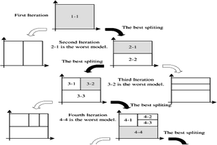
Operational steps for 4 step LOLIMOT algorithm on a two-dimensional input space [20]

Support Vector Machine (SVM).
SVM is one of the supervised methods that provide mapping function from training data, this mapping function can be a classification or regression function. In fact, SVM is a mathematical entity for maximizing a specified math function. For Adjusting SVM learning, considering that there is some unknown and non-linear dependency y = f(x), between the input vector of x with high dimension and a nominal output of y is important [25]. The main idea behind the SVM algorithm needs to use four essential concepts:
-
Separating the hyperplanes. This rule is about drawing a line between clusters. After separating clusters of data, prediction of unknown elements would be easy because the element would be definitely on one side of the separating line, Fig. 5.
Fig. 5. 
Separating data classes by hyperplane [26]

The equation of the separating line can be modified with Eq. 11.
It is considered that data set is like \( \left\{ {{\text{x}}_{\text{i}} , {\text{y}}_{\text{i}} |{\text{i}} = 1,2, \ldots ,{\text{n}}} \right\} \) that \( {\text{x}}_{\text{i}} \in {\mathcal{R}}^{\text{d}} \), \( {\text{y}}_{\text{i}} \in \left\{ { + 1 , - 1} \right\} \) and b is bias parameter (Figs. 6 and 7).

Existence of multiple separating hyperplanes [26]

Choosing the best margin allows risks or errors between margins. The aim of SVM is finding the maximum margin, Eq. 12.
Equations 11 and 12 can lead to Eq. 13 as below [34,35,36,37,38].
-
The soft margin. Many of data sets are not separable with a single straight line. Its causes the SVM dealing with errors and allows falling wrong elements on the wrong side of the separating line. Consequently, for carrying out this issue SVM can add a soft margin without affecting on its final results, Fig. 8.

In addition, we don’t want to allow many wrong classified elements. Describing soft margin has to provide a parameter for the user to determine how many samples can break separating hyperplane rule and how far from that margin they can be located. It’s obvious the tradeoff between both maximum margin and have a correct classification of samples will be complex [17].
In this case, according to Fig. 8, slack variables (\( \upxi_{\text{i}} \)) can use in goal function, Eq. 14. \( {\text{C}}\sum\nolimits_{\text{i}} {\upxi_{\text{i}} } \) Specifies maximum errors [34,35,36,37,38].
With constraints:
-
The kernel function. Sometimes there are inseparable data set and there is no single point that can separate two classes and even there isn’t any separating soft margin [27], Fig. 9.
Fig. 9. 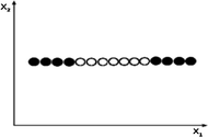
Linear, non-separable data set [26]

Kernel function can solve this problem by adding an additional dimension to the data. For obtaining new dimension, values of the main function are squared. Kernel functions, map data from a lower dimension to a higher dimension by selecting a suitable function. Thus, data set would be separable in a higher dimension space which is called feature space. The feature space in Fig. 9 converted to higher dimension by kernel function in Fig. 10.

Non-separable data set with augmenting new dimension [26]
With kernel functions variable x maps to \( {\upvarphi }\left( {\text{x}} \right), \) Fig. 11.

Mapping data from input space to feature space [40]
It’s provable that there is at least one kernel function for each data set which can separate data sets linearly. Although mapping data to a higher dimension can make some problems like increasing the number of values and possible solutions. Data mapping into excessive higher space causes special boundaries shown in Fig. 12, [34,35,36].

Transferring training data to the higher dimension [26]
Support Vector Regression (SVR).
Support Vector Regression had been used for recognizing patterns, then it has been developed for dealing with non-linear regression problems [28]. SVR model is based on non-linear mapping of main x data to a higher dimension feature space. In fact, SVR is a way of function estimating that maps an input object to a real number base on training data [29]. In SVR, estimating errors are using instead of SVM’s margin. Vapnik’s epsilon error function determines a ε-cylinder [6]. If predicted values were in the cylinder, the error would be zero, but for all out of cylinder, the error would be equal to difference between predicted value and cylinder ε radius, Fig. 13, [16, 24].

Support Vector Regression [30]
Vapnik’s linear loss function with \( \upvarepsilon \) sensitive range defined as Eq. 15, [29].
If SVR algorithm considered soft margin, the Eq. 15, with \( \upxi_{\text{i}} \) the slack variabale would be as Eq. 16.
Fuzzy Membership.
Fuzziness should be used in systems which their information is not precise and certain. A model of a vague phenomenon might be presented as a fuzzy relation that introduced by ‘Lotfi zadeh’. A membership function for a fuzzy set ‘A’, with x statistical population, is s_i:x→ [0,1]. While each \( {\text{x}}_{\text{i}} \) element mapped to a value between 0 and 1. This value is called fuzzy membership, which calculates the amount of element’s membership in a fuzzy set [31,32,33].
Fuzzy Support Vector Methods.
Support vector technologies are strong tools for classification and regression, but there are some restrictions in this theory. In SVM, each training element belongs to just one class. In many applications, some of the input points are not assigned to a specific class. Also, some points, are meaningless due to noises and it is better to ignore them. Considering fuzzy membership for support vector methods make them able to reduce the impacts of noises and outlier data [32, 33].
It can be mentioned that in many real-world applications, training data have different effects, also some of them are more important in classification problems. Therefore, in classification algorithms, meaningful training data, must be classified correctly and classifying or not classifying of some of those points like noises, is not important [41, 42].
In standard SV algorithms, the importance of number of errors for all training elements is considered the same, while it should not be like that. The importance of each element can be calculated with fuzzy logic in training phase, and then instead of hard decision in decision phase, a soft decision can be gained [41, 43].
Local Outlier Factor (LOF).
One of the algorithms for determining outlier points is LOF. This algorithm by comparing local density of an element with local density of its neighbors, can specify areas with same densities or specify elements which have natural lower density. Thus, this algorithm is able to determine outliers in a data set and fuzzy membership of each element is calculated according to that. In this paper, fuzzy membership of each element is calculated with LOF algorithm [44].
4 Experimental Study
Each applied data set has missing values naturally, therefore our goal is to estimate missing values based on 14 missing value imputation methods. 12 of these methods are based on Luengo et al. study. They have been developed a tool called “KEEL” in order to impute and classify incomplete datasets. Our proposed approach is implemented with 2 mentioned methods and also, has been compared with those 12 methods [8].
This section of study, describes the experiments which had been performed for our study. First of all, the incomplete units are imputed in data sets with imputation methods and secondly, the result data sets that are completed are fed to MLP neural network as a classifier. Finally, the classification error on each completed data set which had been imputed by an individual imputation method is compared. This section also included the graphical analysis of these different imputation methods.
4.1 Data Sets
Seven individual data sets had been selected from UCI repository in order to experiment study. The properties of these applied data sets are described in detail in Table 1.
In Table 2, used parameters with their amount, is shown for each algorithm. Determined parameters in Table 2, had best results on used data sets.
4.2 Graphical Analysis of the Classification
Accuracy of All Applied Methods.
Two applied algorithms are compared with 12 other algorithms which are mentioned in previous sections. These figures depict results of all compared methods and indicate rate of correctly classified in each dataset. As which have been shown in figures it is obvious that suggested algorithms have higher range of accuracy based on these datasets Figs. 14, 15, 16, 17, 18, 19 and 20. Also, Figs. 21, 22, 23 and 24 show the differences between the target data and the predicted data by the used methods, i.e., LOLIMOT and FSVM/FSVR, on Wisconsin data set.

Classification accuracy of different methods on Autos dataset.

Classification accuracy of different methods on Cleveland dataset

Classification accuracy of different methods on Mushroom dataset.

Classification accuracy of different methods on Breast dataset

Classification accuracy of different methods on Wisconsin dataset

Classification accuracy of different methods on CRX dataset

Classification accuracy of different methods on Post-operative dataset

Target test data and simulated test data by FSVM/FSVR

Target train data and simulated train data by LOLIMOT

Target train data and simulated train data FSVM/FSVR

Target test data and simulated test data by LOLIMOT
5 Conclusion
Although our proposed approach enforces computational burdens, it delivers high accuracy results. Thus, this approach can be recommended in those studies, that computational complexities can be disregarded.
According to obtained results, it has been recognized that used algorithms in missing data imputation, can model the train data and also predict test data with high precision and high accuracy. LOLIMOT can gain more accuracy by applying divide and conquer strategy and local linear models in order to solve a nonlinear problem. The main reason for precise results of FSVM/FSVR is the usage of fuzzy membership in modelling train data. In addition, finding out a better initializing substantial parameters will result in less computation time. Therefore, finding techniques to indicate better initial parameters can help for better sufficiency. Also, using appropriate preprocessing on different datasets will cause higher authenticity in results. As a suggestion, to indicate better initial parameters and find more appropriate kernel functions, usage of meta-heuristics methods can be useful.
References
Meesad, P., Yen, G.G.: Combined numerical and linguistic knowledge representation and its application to medical diagnosis. In: IEEE Transactions on Systems, Man, and Cybernetics - Part A: Systems and Humans, pp. 206–222, August 2003
Li, D., Deogun, J., Spaulding, W., Shuart, B.: Towards missing data imputation: a study of fuzzy K-means clustering method. In: Tsumoto, S., Słowiński, R., Komorowski, J., Grzymała-Busse, Jerzy W. (eds.) RSCTC 2004. LNCS (LNAI), vol. 3066, pp. 573–579. Springer, Heidelberg (2004). https://doi.org/10.1007/978-3-540-25929-9_70
Schafer, J.L.: Analysis of Incomplete Data, pp. 10–13. Chapman & Hall, London (1997)
Little, R.J., Rubin, D.B.: Statistical Analysis with Missing Data, 2nd edn, pp. 3–19. Wiley, New York (2002)
Wayman, C.: Multiple imputation for missing data: what is it and how can I use it. In: Annual Meeting of the American Educational Research Association, Chicago, IL, pp. 2–16 (2003)
Jiri, K.: Dealing with missing values in data. Faculty of Civil Engineering, Czech Technical University, pp. 1–10 (2013)
Schafer, L.J., Graham, J.W.: Missing data: our view of the state of the art. Psychol. Methods 7(2), 147–177 (2002)
Luengo, J., Garcia, S., Herrera, F.: A study on the use of imputation methods for experimentation with Radial Basis Function Network classifiers handling attribute values: the good synergy between RBFNs and Event Covering method. CITIC-University of Granada, pp. 406–418 (2010)
Grzymała-Busse, J.W., Grzymała-Busse, W.J., Goodwin, L.K.: A closest fit approach to missing attribute values in preterm birth data. In: Zhong, N., Skowron, A., Ohsuga, S. (eds.) RSFDGrC 1999. LNCS (LNAI), vol. 1711, pp. 405–413. Springer, Heidelberg (1999). https://doi.org/10.1007/978-3-540-48061-7_49
Grzymala-Busse, J.W., Hu, M.: A comparison of several approaches to missing attribute values in data mining. In: Ziarko, W., Yao, Y. (eds.) RSCTC 2000. LNCS (LNAI), vol. 2005, pp. 378–385. Springer, Heidelberg (2001). https://doi.org/10.1007/3-540-45554-X_46
Kantardzic, M.: Data Mining-Concepts, Models, Methods, and Algorithms. IEEE, pp. 165–176 (2003)
Site dedicated to missing values: http://sci2s.ugr.es/MVDM/index.php#four, Bibliography on missing values: http://sci2s.ugr.es/MVDM/biblio.php
Little, R.J., Rubin, D.B.: Statistical analysis with missing data, 2nd edn, pp. 1–409. Wiley, Hoboken (2002)
Hand, D.J., Manilla, H., Smyth, P.: Principles of Data Mining, A Bradford Book, pp. 157–160. MIT Press, Cambridge (2001)
Gustavo, E., Monard, B., Monard, M.C.: A Study of K-Nearest Neighbour as an Imputation Method. Institute of Mathematics and Computer Science– ICMC, pp. 1–10 (2002)
Smola, A.J., Scholkophf, B.: A tutorial on Support Vector Regression. NeuroCOLT2 Technical report Series, NC2-TR-1998-03, pp. 1–73, October 1998
Scholkopf, B., Burges, C., Vapnik, V.: Extracting support data for a given task. In: Fayyad, U.M., Uthurusamy, R. (eds.) Proceedings, First International Conference on Knowledge Discovery and Data Mining, pp. 252–257. AAAI Press, Menlo Park (1995)
Chen, Z.: Data Mining and Uncertain Reasoning: An Integrated Approach, pp. 1–392. Wiley, Hoboken (2001)
Fahlman, S.E., Lebiere, C.: The cascade-correlation learning architecture. In: Touretzky, D.S. (ed.) Advances in Neural Information Processing Systems 2, pp. 1–17. Morgan-Kaufmann, Los Altos (1990)
Nelles, O.: Nonlinear System Identification, pp. 69–341. Springer, New York (2001). https://doi.org/10.1007/978-3-662-04323-3
Sohani, M., Kermani, K.K.: A neuro-fuzzy approach to diagnosis of neonatal jaundice. In: Proceedings of the 1st International Conference on Bio Inspired Models of Network, Information and Computing Systems Cavalese, Italy, pp. 2–6 (2006)
Janghorbani, A., Arasteh, A.: Application of local linear neuro-fuzzy model in prediction of mean arterial blood pressure time series. In: Proceedings of the 17th Iranian Conference of Biomedical Engineering (ICBME 2010), pp. 1–4 (2010)
Nikookar, A., Lucas, C.: Artificial bee colony based learning of local linear neuro-fuzzy models. In: IEEE Fuzzy Systems (IFSC), pp. 1–4 (2013)
Sen, W., Hong, C., Xiaodong, F.: Clustering algorithm for incomplete data sets with mixed numerical and categorical attributes. Int. J. Database Theory Appl. 6(5), 95–104 (2013)
Wang, L. (ed.): Support Vector Machines: Theory and Applications, pp. 1–434. Springer, Heidelberg (2005). https://doi.org/10.1007/b95439
Nobel, W.S.: What is a support vector machine? Comput. Biol. 1–3 (2006)
Pigott, T.D.: A review of methods for missing data. Educ. Res. Eval. 7(4), 353–383 (2001)
Vapnik, V., Golowich, S., Smola, A.: Support vector machine for function approximation regression estimation and signal processing. In: Advances in Neural Information Processing Systems, vol. 9, pp. 281–287 (1996)
Yu, H., Kim, S.: SVM tutorial — classification, regression and ranking. In: Rozenberg, G., Bäck, T., Kok, J.N. (eds.) Handbook of Natural Computing, pp. 479–506. Springer, Heidelberg (2012). https://doi.org/10.1007/978-3-540-92910-9_15
Enders, C.: Applied Missing Data Analysis, pp. 3–55. Guilford Press, New York (2010)
Luengo, J., Garcia, S., Herrera, F.: On the choice of the best imputation methods for missing values considering three groups of classification methods. Knowl. Inf. Syst. 32, 77–108 (2011)
http://faradars.org/courses/mvrnn9102fh-support-vector-machine-in-matlab-video-tutorial
Learning: Support Vector Machines. https://www.youtube.com/watch?v=PwhiWxHK8o
5 Minutes with Ingo: Understanding Support Vector Machines. https://www.youtube.com/watch?v=YsiWisFFruY
Bottou, l., et al.: Comparison of classifier methods: a case study in handwritten digit recognition. In: Proceedings of the 12th IAPR International Conference on Pattern Recognition, vol. 2, pp. 77–82, 9–13 October 1994
Vapnik, V.: The Nature of Statistical Learning Theory, 2nd edn, pp. 1–314. Springer, New York (2000). https://doi.org/10.1007/978-1-4757-3264-1
Liao, R.: Support Vector Machines, pp. 1–33, 10 November 2015
Lin, C., Wang, S.: Fuzzy support vector machines. IEEE Trans. Neural Netw. 13(2), 464–471 (2002)
Lin, K., Pai, P.: A fuzzy support vector regression model for business cycle predictions. Expert Syst. Appl. 37, 5430–5435 (2010)
Huang, H., Liu, Y.: Fuzzy support vector machines for pattern recognition and data mining. Int. J. Fuzzy Syst. 4(3), 826–835 (2002)
Local outlier factor. https://en.wikipedia.org/wiki/Local_outlier_factor
Author information
Authors and Affiliations
Corresponding authors
Editor information
Editors and Affiliations
Rights and permissions
Copyright information
© 2018 Springer International Publishing AG, part of Springer Nature
About this paper

Cite this paper
Fazlikhani, F., Motakefi, P., Pedram, M.M. (2018). Missing Data Imputation by LOLIMOT and FSVM/FSVR Algorithms with a Novel Approach: A Comparative Study. In: Medina, J., et al. Information Processing and Management of Uncertainty in Knowledge-Based Systems. Theory and Foundations. IPMU 2018. Communications in Computer and Information Science, vol 854. Springer, Cham. https://doi.org/10.1007/978-3-319-91476-3_46
Download citation
DOI: https://doi.org/10.1007/978-3-319-91476-3_46
Published:
Publisher Name: Springer, Cham
Print ISBN: 978-3-319-91475-6
Online ISBN: 978-3-319-91476-3
eBook Packages: Computer ScienceComputer Science (R0)