
Abstract
We present simpler and improved constructions of unbounded attribute-based encryption (ABE) schemes with constant-size public parameters under static assumptions in bilinear groups. Concretely, we obtain:
-
a simple and adaptively secure unbounded ABE scheme in composite-order groups, improving upon a previous construction of Lewko and Waters (Eurocrypt ’11) which only achieves selective security;
-
an improved adaptively secure unbounded ABE scheme based on the k-linear assumption in prime-order groups with shorter ciphertexts and secret keys than those of Okamoto and Takashima (Asiacrypt ’12);
-
the first adaptively secure unbounded ABE scheme for arithmetic branching programs under static assumptions.
At the core of all of these constructions is a “bilinear entropy expansion” lemma that allows us to generate any polynomial amount of entropy starting from constant-size public parameters; the entropy can then be used to transform existing adaptively secure “bounded” ABE schemes into unbounded ones.
J. Chen—School of Computer Science and Software Engineering. Supported by the National Natural Science Foundation of China (Nos. 61472142, 61632012, U1705264) and the Young Elite Scientists Sponsorship Program by CAST (2017QNRC001). Homepage: http://www.jchen.top.
J. Gong—Supported in part by the French ANR ALAMBIC Project (ANR-16-CE39-0006).
L. Kowalczyk—Supported in part by an NSF Graduate Research Fellowship DGE-16-44869; The Leona M. & Harry B. Helmsley Charitable Trust; ERC Project aSCEND (H2020 639554); the Defense Advanced Research Project Agency (DARPA) and Army Research Office (ARO) under Contract W911NF-15-C-0236; and NSF grants CNS-1445424, CNS-1552932 and CCF-1423306. Any opinions, findings and conclusions or recommendations expressed are those of the authors and do not necessarily reflect the views of the Defense Advanced Research Projects Agency, Army Research Office, the National Science Foundation, or the U.S. Government.
H. Wee—Supported in part by ERC Project aSCEND (H2020 639554), H2020 FENTEC and NSF Award CNS-1445424.
You have full access to this open access chapter, Download conference paper PDF
1 Introduction
Attribute-based encryption (ABE) [13, 25] is a generalization of public-key encryption to support fine-grained access control for encrypted data. Here, ciphertexts and keys are associated with descriptive values which determine whether decryption is possible. In a key-policy ABE (KP-ABE) scheme for instance, ciphertexts are associated with attributes like ‘(author:Waters), (inst:UT), (topic:PK)’ and keys with access policies like ‘((topic:MPC) OR (topic:Qu)) AND (NOT(inst:CWI))’, and decryption is possible only when the attributes satisfy the access policy. A ciphertext-policy (CP-ABE) scheme is the dual of KP-ABE with ciphertexts associated with policies and keys with attributes.
Over past decade, substantial progress has been made in the design and analysis of ABE schemes, leading to a large families of schemes that achieve various trade-offs between efficiency, security and underlying assumptions. Meanwhile, ABE has found use as a tool for providing and enhancing privacy in a variety of settings from electronic medical records to messaging systems and online social networks.
As institutions grow and with new emerging and more complex applications for ABE, it became clear that we need ABE schemes that can readily accommodate the addition of new roles, entities, attributes and policies. This means that the ABE set-up algorithm should put no restriction on the length of the attributes or the size of the policies that will be used in the ciphertexts and keys. This requirement was introduced and first realized in the work of Lewko and Waters [21] under the term unbounded ABE. Their constructions have since been improved and extended in several subsequent works [1,2,3, 5, 12, 17, 18, 23, 24] (cf. Figs. 1 and 2).
In this work, we put forth new ABE schemes that simultaneously:
-
(1)
are unbounded (the set-up algorithm is independent of the length of the attributes or the size of the policies);
-
(2)
can be based on faster asymmetric prime-order bilinear groups;
-
(3)
achieve adaptive security;
-
(4)
rely on simple hardness assumptions in the standard model.
All four properties are highly desirable from both a practical and theoretical stand-point and moreover, properties (1)–(3) are crucial for many real-world applications of ABE. Indeed, properties (2), (3) and (4) are by now standard cryptographic requirements pertaining to speed and efficiency, strong security guarantees under realistic and natural attack models, and minimal hardness assumptions. Property (2) is additionally motivated by the fact that pairing-based schemes are currently more widely implemented and deployed than lattice-based ones. There is now a vast body of works (e.g. [2, 3, 6, 19, 22, 27]) showing how to achieve properties (2)–(4) for “bounded” ABE where the set-up time and public parameters grow with the attributes or policies, culminating in unifying frameworks that provide a solid understanding of the design and analysis of these schemes. Unbounded ABE, on the other hand, has received comparatively much less attention in the literature; this is in part because the schemes and proofs remain fairly complex and delicate. Amongst these latter works, only the work of Okamato and Takashima (OT) [23] simultaneously achieved (1)–(4).
Our Results. We present simpler and more modular constructions of unbounded ABE that realize properties (1)–(4) with better efficiency and expressiveness than was previously known.
-
(i)
We present new adaptively secure, unbounded KP-ABE schemes for monotone span programs –which capture access policies computable by monotone Boolean formulas– whose ciphertexts are 42% smaller and our keys are 8% smaller than the state-of-the-art in [23] (with even more substantial savings with our SXDH-based scheme), as well as CP-ABE schemes with similar savings, cf. Fig. 3.
-
(ii)
Our constructions generalize to the larger class of arithmetic span programs [15], which capture many natural computational models, such as monotone Boolean formulas, as well as Boolean and arithmetic branching programs; this yields the first adaptively secure, unbounded KP-ABE for arithmetic span programs. Prior to this work, we do not even know any selectively secure, unbounded KP-ABE for arithmetic span programs.
Moreover, our constructions generalize readily to the k-Lin assumption.

Summary of unbounded KP-ABE schemes for monotone span programs from prime-order groups with O(1)-size \(\textsf {mpk}\).

Summary of unbounded KP-ABE schemes for monotone span programs with n-bit attributes (i.e. universe [n]) from composite-order groups.

Summary of adaptively secure, unbounded ABE schemes for read-once monotone span programs with n-bit attributes (i.e. universe [n]) from prime-order groups. The columns \(| \mathsf {sk}|\) and \(| \mathsf {ct}|\) refer to the number of group elements in \(G_2\) and \(G_1\) respectively (minus a \(|G_T|\) contribution in \( \mathsf {ct}\)).
At the core of all of these constructions is a “bilinear entropy expansion” lemma [17] that allows us to generate any polynomial amount of entropy starting from constant-size public parameters; the entropy can then be used to transform existing adaptively secure bounded ABE schemes into unbounded ones in a single shot. The fact that we only need to invoke our entropy expansion lemma once yields both quantitative and qualitative advantages over prior works [17, 23]: (i) we achieve security loss \(O(n+Q)\) for n-bit attributes (i.e. universe [n]) and Q secret key queries, improving upon \(O(n \cdot Q)\) in [23] and \(O(\log n \cdot Q)\) in [17] and (ii) there is clear delineation between entropy expansion and the analysis of the underlying bounded ABE schemes, whereas prior works interweave both techniques in a more complex nested manner.
Following the recent literature on adaptively secure bounded ABE, we first describe our constructions in the simpler setting of composite-order bilinear groups, and then derive our final prime-order schemes by building upon and extending previous frameworks in [6, 7, 11]. Along the way, we also present a simple adaptively secure unbounded KP-ABE scheme in composite-order groups whose hardness relies on standard, static assumptions (cf. Fig. 2).
1.1 Technical Overview
We will start with asymmetric composite-order bilinear groups \((G_N,H_N,G_T)\) whose order N is the product of three primes \(p_1,p_2,p_3\). Let \(g_i,h_i\) denote generators of order \(p_i\) in \(G_N\) and \(H_N\), for \(i=1,2,3\).
Warm-Up. We begin with the LOSTW KP-ABE for monotone span programs [19]; this is a bounded, adaptively secure scheme that uses composite-order groups. Here, ciphertexts \( \mathsf {ct}_\mathbf {x}\) are associated with attribute vectorFootnote 1 \(\mathbf {x}\in \{0,1\}^n\) and keys \( \mathsf {sk}_\mathbf {M}\) with read-once monotone span programs \(\mathbf {M}\).Footnote 2
where \(\alpha _1,\ldots ,\alpha _n\) are shares of \(\alpha \) w.r.t. the span program \(\mathbf {M}\); the shares satisfy the requirement that for any \(\mathbf {x}\in \{0,1\}^n\), the shares \(\{ \alpha _j \}_{x_j = 1}\) determine \(\alpha \) if \(\mathbf {x}\) satisfies \(\mathbf {M}\), and reveal nothing about \(\alpha \) otherwise. For decryption, observe that we can compute \(\{ e(g_1,h_1)^{\alpha _j s} \}_{x_j=1}\), from which we can compute the blinding factor \(e(g_1,h_1)^{\alpha s}\). The proof of security relies on Waters’ dual system encryption methodology [2, 20, 26, 27], in the most basic setting at the core of which is an information-theoretic statement about \(\alpha _j,v_j\).
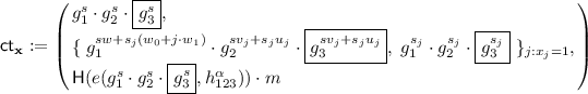
Towards Our Unbounded ABE. The main challenge in building an unbounded ABE lies in “compressing” \(g_1^{v_1},\ldots ,g_1^{v_n}\) in \(\textsf {mpk}\) down to a constant number of group elements. The first idea following [21, 23] is to generate \(\{v_j\}_{j \in [n]}\) via a pairwise-independent hash function as \(w_0+j \cdot w_1\), as in the Lewko-Waters IBE. Simply replacing \(v_j\) with \(w_0+j \cdot w_1\) leads to natural malleability attacks on the ciphertext, and instead, we would replace \(sv_j \) with \(s_j(w_0+j \cdot w_1)\), where \(s_1,\ldots ,s_n\) are fresh randomness used in encryption. Next, we need to bind the \(s_j(w_0+j \cdot w_1)\)’s together via some common randomness s; it suffices to use \(sw+s_j(w_0+j \cdot w_1)\) in the ciphertext. That is, we start with the scheme in (1) and we perform the substitutions (*) for each \(j \in [n]\):
This yields the following scheme:
As a sanity check for decryption, observe that we can compute \(\{ e(g_1,h_1)^{\alpha _j s} \}_{x_j=1}\) and then \(e(g_1,h_1)^{\alpha s}\) as before. We note that the ensuing scheme is similar to Attrapadung’s unbounded KP-ABE in [2, Sect. 7.1], except the latter requires q-type assumptions.Footnote 3
Our Proof Strategy. To analyze our scheme in (2), we follow a very simple and natural proof strategy: we would “undo” the substitutions described in (*) to recover ciphertext and keys similar to those in the LOSTW KP-ABE, upon which we could apply the analysis for the bounded setting from the prior works. That is, we want to computationally replace each \(w_0 + j\cdot w_1\) with a fresh \(u_j\):

Unfortunately, once we give out \(g_1^{w_0},g_1^{w_1}\) in \(\textsf {mpk}\), the above distributions are trivially distinguishable by using the relation \(e(g_1,h_1^{r_j(w_0+j\cdot w_1)}) = e(g_1^{w_0+j\cdot w_1},h_1^{r_j})\). Furthermore, the above statement does not yield a scheme similar to LOSTW when applied to our scheme in (2); for that, we would need to also replace w on the RHS in (3) with fresh \(v_j\) as described by
in order to match up with the LOSTW KP-ABE in (1).
1.2 Bilinear Entropy Expansion
The core of our analysis is a (bilinear) entropy expansion lemma [17] that captures the spirit of the above statement in (3), namely, it allows us to generate fresh independent randomness starting from the correlated randomness, albeit in a new subgroup of order \(p_2\) generated by \(g_2,h_2\).
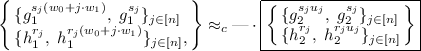
More formally, given public parameters \((g_1,g_1^w,g_1^{w_0},g_1^{w_1}, h_1,h_1^w,h_1^{w_0},h_1^{w_1})\), we show that

where “—” is short-hand for duplicating the terms on the LHS, so that the \(g_1,h_1\)-components remain unchanged. That is, starting with the LHS, we replaced (i) \(w_0+j \cdot w_1\) with fresh \(u_j\), and (ii) w with fresh \(v_j\), both in the \(p_2\)-subgroup. We also omitted the \(\alpha _j\)’s from (3). We clarify that the trivial distinguisher on (3) fails here because \(e(g_1,h_2)=1\).
Prior Work. We clarify that the name “bilinear entropy expansion” was introduced in the prior work of Kowalczyk and Lewko (KL) [17], which also proved a statement similar to (3), with three notable differences: (i) our entropy expansion lemma starts with 3 units of entropy \((w,w_0,w_1)\) whereas KL uses \(O(\log n)\) units of entropy; (ii) the KL statement does not account for the public parameters, and therefore (unlike our lemma) cannot serve as an immediate bridge from the unbounded ABE to the bounded variant; (iii) our entropy expansion lemma admits an analogue in prime-order groups, which in turn yields an unbounded ABE scheme in prime-order groups, whereas the composite-order ABE scheme in KL does not have an analogue in prime-order setting (an earlier prime-order construction was retracted on June 1, 2016). In fact, the “consistent randomness amplification” techniques used in the unbounded ABE schemes of Okamoto and Takashima (OT) [23] also seem to yield an entropy expansion lemma with O(1) units of entropy in prime-order groups. As noted earlier in the introduction, our approach is also different from both KL and OT in the sense that we only need to invoke our entropy expansion lemma once when proving security of the unbounded ABE.
Proof Overview. We provide a proof overview of our entropy expansion lemma in (4). The proof proceeds in two steps: (i) replacing \(w_0 + j \cdot w_1\) with fresh \(u_j\), and then (ii) replacing w with fresh \(v_j\).
-
(i)
We replace \(w_0+j \cdot w_1\) with fresh \(u_j\); that is,
 (5)
(5)where we suppressed the terms involving w; moreover, this holds even given \(g_1, g_1^{w_0}, g_1^{w_1}\). Our first observation is that we can easily adapt the proof of Lewko-Waters IBE [8, 20] to show that for each \(i \in [n]\),
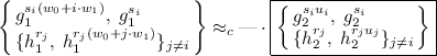 (6)
(6)The idea is that the first term on the LHS corresponds to an encryption for the identity i, and the next \(n-1\) terms correspond to secret keys for identities \(j \ne i\); on the right, we have the corresponding “semi-functional entities”. At this point, we can easily handle \((h_2^{r_i}, h_2^{r_i(w_0 + i\cdot w_1)})\) via a statistical argument, thanks to the entropy in \(w_0 + i\cdot w_1 \bmod p_2\). Next, we need to get from a single \((g_{1}^{s_i(w_0+i\cdot w_1)},\; g_{1}^{s_i})\) on the LHS in (6) to n such terms on the LHS in (5). This requires a delicate “two slot” hybrid argument over \(i \in [n]\) and the use of an additional subgroup; similar arguments also appeared in [14, 23]. This is where we used the fact that N is a product of three primes, whereas the Lewko-Waters IBE and the statement in (6) works with two primes in the asymmetric setting.
-
(ii)
Next, we replace w with fresh \(v_j\); that is,
$$ \left\{ \begin{array}{llll} g_2^{s},\;\{ g_{2}^{sw + s_ju_j},\; g_{2}^{s_j}\}_{j \in [n]} \\ \{ h_{2}^{r_j w}, \; h_{2}^{r_j}, \; h_2^{r_ju_j}\}_{j \in [n]} \end{array} \right\} \approx _c \left\{ \begin{array}{llll} g_2^s,\;\{ g_{2}^{sv_j + s_ju_j},\; g_{2}^{s_j}\}_{j \in [n]} \\ \{ h_{2}^{r_j v_j}, \; h_{2}^{r_j}, \; h_2^{r_ju_j}\}_{j \in [n]} \end{array} \right\} $$Intuitively, this should follow from the DDH assumption in the \(p_2\)-subgroup, which says that \((h_2^{r_jw}, h_2^{r_j}) \approx _c (h_2^{r_jv_j}, h_2^{r_j})\). The actual proof is more delicate since w also appears on the other side of the pairing as \(g_2^{sw + s_ju_j}\); fortunately, we can treat \(u_j\) as a one-time pad that masks w.


Completing the Proof of Unbounded ABE. We return to a proof sketch of our unbounded ABE in (2). Let us start with the simpler setting where the adversary makes only a single key query. Upon applying our entropy expansion lemmaFootnote 4, we have that the ciphertext/key pair \(( \mathsf {ct}_\mathbf {x}, \mathsf {sk}_\mathbf {M})\) satisfies

with \(e(g_1,h_1)^{\alpha s} \cdot m\) omitted. Note that the boxed term on the RHS is exactly the LOSTW KP-ABE ciphertext/key pair in (1) over the \(p_2\)-subgroup, once we strip away the terms involving \(u_j,s_j\).
Finally, to handle the general setting where the ABE adversary makes Q key queries, we simply observe that thanks to self-reducibility, our entropy expansion lemma extends to a Q-fold setting (with Q copies of \(\{r_j\}_{j \in [n]}\)) without any additional security loss:

At this point, we can rely on the (adaptive) security for the LOSTW KP-ABE for the setting with a single challenge ciphertext and Q key queries.
1.3 Our Prime-Order Scheme
To obtain prime-order analogues of our composite-order schemes, we build upon and extend the previous framework of Chen et al. [6, 11] for simulating composite-order groups in prime-order ones. Along the way, we present a more general framework that provides prime-order analogues of the static assumptions used in the security proof for our composite-order ABE. Moreover, we show that these prime-order analogues follow from the standard k-Linear assumption (and more generally, the MDDH assumption [9]) in prime-order bilinear groups.
Our KP-ABE. Let \((G_1,G_2,G_T)\) be a bilinear group of prime order p. Following [6, 11], we start with our composite-order KP-ABE scheme in (2), sample \(\mathbf {A}_1 \leftarrow _{\textsc {r}}\mathbb {Z}_p^{(2k+1) \times k}, \mathbf {B}\leftarrow _{\textsc {r}}\mathbb {Z}_p^{(k+1) \times k}\), and carry out the following substitutions:

where \([\cdot ]_1,[\cdot ]_2\) correspond respectively to exponentiations in the prime-order groups \(G_1,G_2\). This yields the following prime-order KP-ABE scheme for monotone span programs:

where \(\mathbf {k}_j\) is the j’th share of \(\mathbf {k}\). Decryption proceeds as before by first computing \(\{ e([\mathbf {s}^{\top }\mathbf {A}_1^{\top }]_1,[\mathbf {k}_j]_2) \}_{x_j = 1}\) and relies on the associativity relations \(\mathbf {A}_1^{\top }\mathbf {W}\cdot \mathbf {B}= \mathbf {A}_1^{\top }\cdot \mathbf {W}\mathbf {B}\) (ditto \(\mathbf {W}_0+j\cdot \mathbf {W}_1\)) [7].
Dimensions of \(\mathbf {A}_1,\mathbf {B}\mathbf{. }\) It is helpful to compare the dimensions of \(\mathbf {A}_1,\mathbf {B}\) to those of the CGW prime-order analogue of LOSTW in [6]; once we fix the dimensions of \(\mathbf {A}_1,\mathbf {B}\), the dimensions of \(\mathbf {W},\mathbf {W}_0,\mathbf {W}_1\) are also fixed. In all of these constructions, the width of \(\mathbf {A}_1,\mathbf {B}\) is always k, for constructions based on the k-linear assumption. CGW uses a shorter \(\mathbf {A}_1\) of dimensions \((k+1) \times k\), and a \(\mathbf {B}\) of the same dimensions \((k+1) \times k\). Roughly speaking, increasing the height of \(\mathbf {A}_1\) by k plays the role of adding a subgroup in our composite-order scheme; in particular, the LOSTW KP-ABE uses a group of order \(p_1p_2\) in the asymmetric setting, whereas our unbounded ABE uses a group of order \(p_1p_2p_3\).
We note that the direct adaptation of the prior techniques in [11] would yield \(\mathbf {A}_1\) of height 3k and \(\mathbf {B}\) of height \(k+1\), and reducing the height of \(\mathbf {A}_1\) down to \(2k+1\) is the key to our efficiency improvements over the prime-order unbounded KP-ABE scheme in [23]. To accomplish this, we need to optimize on the static assumptions used in the composite-order bilinear entropy expansion lemma, and thereafter, carefully transfer these optimizations to the prime-order setting, building upon and extending the recent prime-order IBE schemes in [11].
Bilinear Entropy Expansion Lemma. In the rest of this overview, we motivate the prime-order analogue of our bilinear entropy expansion lemma in (4), and defer a more accurate treatment to Sect. 6. Upon our substitutions in (7), we expect to prove a statement of the form:

given also the public parameters \([\mathbf {A}_1^{\top }]_1,[\mathbf {A}_1^{\top }\mathbf {W}]_1,[\mathbf {A}_1^{\top }\mathbf {W}_0]_1,[\mathbf {A}_1^{\top }\mathbf {W}_1]_1\). Here, \(\mathbf {A}_2 \leftarrow _{\textsc {r}}\mathbb {Z}_p^{(2k+1) \times k}\) is an additional matrix that plays the role of \(g_2\), whereas \(\mathbf {U}_j,\mathbf {V}_j\) play the roles of the fresh entropy \(u_j,v_j\). Note that we do not introduce additional terms that correspond to those involving \(h_2\) on the RHS, and can therefore keep \(\mathbf {B}\) of dimensions \((k+1) \times k\). To prevent a trivial distinguishing attack based on the associativity relation \(\mathbf {A}_1^{\top }\mathbf {W}\cdot \mathbf {B}= \mathbf {A}_1^{\top }\cdot \mathbf {W}\mathbf {B}\), we need to sample random \(\mathbf {U}_j,\mathbf {V}_j\) subject to the constraints \(\mathbf {A}_1^{\top }\mathbf {U}_j = \mathbf {A}_1^{\top }\mathbf {V}_j = \mathbf {0}\). In the proof of the entropy expansion lemma, we will show that the k-Lin assumption implies

To complete the proof of the unbounded ABE, we proceed as before in the composite-order setting, and observe that the boxed term in (8) above (once we strip away the terms involving \(\mathbf {U}_j\) and \(\hat{\mathbf {s}}_j\)) correspond to the prime-order variant of the LOSTW KP-ABE in CGW, as given by:
As in the composite-order setting, we need to first extend our bilinear entropy expansion lemma to a Q-fold setting via random self-reducibility. We may then carry out the analysis in CGW to complete the proof of our unbounded ABE.
1.4 Extensions
Due to lack of space, we briefly sketch two extensions: CP-ABE for monotone span programs, and KP-ABE for arithmetic span programs.
CP-ABE. Here, we start with the LOSTW CP-ABE for monotone span programs [19], which basically reverses the structures of the ciphertexts and keys. This means that we will need a variant of our entropy expansion lemma that accommodates a similar reversal. The statement adapts naturally to this setting, and so does the proof, except we need to make some changes to step two, which requires that we start with a taller \(\mathbf {A}_1 \in \mathbb {Z}_q^{3k \times k}\). This gives rise to the following prime-order CP-ABE:

where \(\mathbf {c}_{0,j}\) is the j’th share of \(\mathbf {c}_0 := \mathbf {s}^{\top }\mathbf {A}_1^{\top }\mathbf {U}_0\) w.r.t. \(\mathbf {M}\). Decryption proceeds by first computing \(\{ e([\mathbf {c}_{0,j}^{\top }]_1,[\mathbf {B}\mathbf {r}]_2) \}_{x_j=1}\) and then \(e([\mathbf {c}_0^{\top }]_1,[\mathbf {B}\mathbf {r}]_2)\).
Arithmetic Span Programs. In arithmetic span programs, the attributes \(\mathbf {x}\) come from \(\mathbb {Z}_p^n\) instead of \(\{0,1\}^n\), which enable richer and more expressive arithmetic computation. The analogue of the LOSTW KP-ABE for arithmetic span programs [6, 15] will then have ciphertexts:
That is, we replaced \(g_1^{x_jv_j s}\) in (1) with \(g_1^{(v_j + x_jv'_j )s}\). In the unbounded setting, we will need to generate \(\{v_j\}_{j \in [n]}\) and \(\{v'_j\}_{j \in [n]}\) via two different pairwise-independent hash functions, given by \(w_0 + j \cdot w_1\) and \(w'_0 + j \cdot w'_1\) respectively. Our entropy expansion lemma generalizes naturally to this setting.
2 Preliminaries
Notation. We denote by \(s \leftarrow _{\textsc {r}}S\) the fact that s is picked uniformly at random from a finite set S. By PPT, we denote a probabilistic polynomial-time algorithm. Throughout this paper, we use \(1^\lambda \) as the security parameter. We use lower case boldface to denote (column) vectors and upper case boldcase to denote matrices. We use \(\equiv \) to denote two distributions being identically distributed, and \(\approx _c\) to denote two distributions being computationally indistinguishable. For any two finite sets (also including spaces and groups) \(S_1\) and \(S_2\), the notation “\(S_1 \approx _c S_2\)” means the uniform distributions over them are computationally indistinguishable.
2.1 Monotone Span Programs
We define (monotone) span programs [16].
Definition 1
(span programs [4, 16]). A (monotone) span program for attribute universe [n] is a pair \((\mathbf {M},\rho )\) where \(\mathbf {M}\) is a \(\ell \times {\ell '}\) matrix over \(\mathbb {Z}_p\) and \(\rho : [\ell ] \rightarrow [n]\). Given \(\mathbf {x}= (x_1,\ldots ,x_n)\in \{0,1\}^n\), we say that
Here, \(\mathbf {1} := (1,0,\ldots ,0)^{\top }\in \mathbb {Z}^{1 \times {\ell '}}\) is a row vector; \(\mathbf {M}_\mathbf {x}\) denotes the collection of vectors \(\{ \mathbf {M}_j : x_{\rho (j)} = 1 \}\) where \(\mathbf {M}_j\) denotes the j’th row of \(\mathbf {M}\); and \(\mathsf {span}\) refers to linear span of collection of (row) vectors over \(\mathbb {Z}_p\).
That is, \(\mathbf {x}\) satisfies \((\mathbf {M},\rho )\) if f there exists constants \(\omega _1,\ldots ,\omega _\ell \in \mathbb {Z}_p\) such that
Observe that the constants \(\{\omega _j\}\) can be computed in time polynomial in the size of the matrix \(\mathbf {M}\) via Gaussian elimination. Like in [6, 19], we need to impose a one-use restriction, that is, \(\rho \) is a permutation and \(\ell = n\). By re-ordering the rows of \(\mathbf {M}\), we may assume WLOG that \(\rho \) is the identity map, which we omit in the rest of this section.
Lemma 1
(statistical lemma [6, Appendix A.6]). For any \(\mathbf {x}\) that does not satisfy \(\mathbf {M}\), the distributions
perfectly hide \(\alpha \), where the randomness is taken over \(v_j \leftarrow _{\textsc {r}}\mathbb {Z}_p, \mathbf {u}\leftarrow _{\textsc {r}}\mathbb {Z}_p^{{\ell '}-1}\), and for any fixed \(r_j \ne 0\).
2.2 Attribute-Based Encryption
An attribute-based encryption (ABE) scheme for a predicate \(\mathsf {P}(\,\cdot \,,\,\cdot \,)\) consists of four algorithms \((\mathsf {Setup}, \mathsf {Enc},\) \(\mathsf {KeyGen}, \mathsf {Dec})\):
-
\(\mathsf {Setup}(1^\lambda ,\mathcal {X},\mathcal {Y},\mathcal {M})\rightarrow (\textsf {mpk}, \textsf {msk})\). The setup algorithm gets as input the security parameter \(\lambda \), the attribute universe \(\mathcal {X}\), the predicate universe \(\mathcal {Y}\), the message space \(\mathcal {M}\) and outputs the public parameter \(\textsf {mpk}\), and the master key \(\textsf {msk}\).
-
\(\mathsf {Enc}(\textsf {mpk},x,m)\rightarrow \mathsf {ct}_x\). The encryption algorithm gets as input \(\textsf {mpk}\), an attribute \(x \in \mathcal {X}\) and a message \(m\in \mathcal {M}\). It outputs a ciphertext \( \mathsf {ct}_{x}\). Note that x is public given \( \mathsf {ct}_x\).
-
\(\mathsf {KeyGen}(\textsf {mpk},\textsf {msk},y)\rightarrow \mathsf {sk}_{y}\). The key generation algorithm gets as input \(\textsf {msk}\) and a value \(y \in \mathcal {Y}\). It outputs a secret key \( \mathsf {sk}_{y}\). Note that y is public given \( \mathsf {sk}_y\).
-
\(\mathsf {Dec}(\textsf {mpk}, \mathsf {sk}_{y}, \mathsf {ct}_x ) \rightarrow m\). The decryption algorithm gets as input \( \mathsf {sk}_y\) and \( \mathsf {ct}_x\) such that \(\mathsf {P}(x,y)=1\). It outputs a message m.
Correctness. We require that for all \((x,y) \in \mathcal {X}\times \mathcal {Y}\) such that \(\mathsf {P}(x,y)=1\) and all \(m\in \mathcal {M}\),
where the probability is taken over \((\textsf {mpk},\textsf {msk}) \leftarrow \mathsf {Setup}(1^\lambda ,\mathcal {X},\mathcal {Y},\mathcal {M})\), \( \mathsf {sk}_{y}\leftarrow \mathsf {KeyGen}(\textsf {mpk},\textsf {msk},y)\), and the coins of \(\mathsf {Enc}\).
Security Definition. For a stateful adversary \(\mathcal {A}\), we define the advantage function
with the restriction that all queries y that \(\mathcal {A}\) makes to \(\mathsf {KeyGen}(\textsf {msk},\cdot )\) satisfies \(\mathsf {P}(x^*,y) = 0\) (that is, \( \mathsf {sk}_y\) does not decrypt \( \mathsf {ct}_{x^*}\)). An ABE scheme is adaptively secure if for all PPT adversaries \(\mathcal {A}\), the advantage \(\mathsf {Adv}^{\textsc {abe}}_{\mathcal {A}}(\lambda )\) is a negligible function in \(\lambda \).
Unbounded ABE. An ABE scheme is unbounded [21] if the running time of \(\mathsf {Setup}\) only depends on \(\lambda \); otherwise, we say that it is bounded.
3 Bilinear Entropy Expansion, Revisited
3.1 Composite-Order Bilinear Groups and Computational assumptions
A generator \(\mathcal {G}\) takes as input a security parameter \(\lambda \) and outputs \(\mathbb {G} := (G_N,H_N,G_T,e)\), where N is product of three primes \(p_1,p_2,p_3\) of \(\varTheta (\lambda )\) bits, \(G_N\), \(H_N\) and \(G_T\) are cyclic groups of order N and \(e:G_N\times H_N \rightarrow G_T\) is a non-degenerate bilinear map. We require that the group operations in \(G_N\), \(H_N\) and \(G_T\) as well the bilinear map e are computable in deterministic polynomial time with respect to \(\lambda \). We assume that a random generator g (resp. h) of \(G_N\) (resp. \(H_N\)) is always contained in the description of bilinear groups. For every divisor n of N, we denote by \(G_n\) the subgroup of \(G_N\) of order n. We use \(g_1,g_2,g_3\) to denote random generators of the subgroups \(G_{p_1},G_{p_2},G_{p_3}\) respectively. We define \(h_1,h_2,h_3\) random generators of the subgroups \(H_{p_1},H_{p_2},H_{p_3}\) analogously.
Computational Assumptions. We review two static computational assumptions in the composite-order group, used e.g. in [8, 20].
Assumption 1
( \(\mathbf {SD}^{G_N}_{p_{1} \mapsto p_{1}p_{2}}\) ). We say that \((p_1 \mapsto p_1p_2)\)-subgroup decision assumption, denoted by \(\text {SD}^{G_N}_{p_{1} \mapsto p_{1}p_{2}}\), holds if for all PPT adversaries \(\mathcal {A}\), the following advantage function is negligible in \(\lambda \).
where

Assumption 2
( \(\mathbf {DDH}^{H_N}_{p_{1}}\) ). We say that \(p_1\)-subgroup Diffie-Hellman assumption, denoted by \(\text {DDH}^{H_N}_{p_{1}}\), holds if for all PPT adversaries \(\mathcal {A}\), the following advantage function is negligible in \(\lambda \).
where

By symmetry, one may permute the indices for subgroups and/or exchange the roles of \(G_N\) and \(H_N\), and define \(\text {SD}^{G_N}_{p_{1} \mapsto p_{1}p_{3}}\), \(\text {SD}^{G_N}_{p_{3} \mapsto p_{3}p_{2}}\), SD\(^{H_N}_{p_1\mapsto p_1p_2}\), \(\text {SD}^{H_N}_{p_{1} \mapsto p_{1}p_{3}}\) and \(\text {DDH}^{H_N}_{p_{2}},\text {DDH}^{H_N}_{p_{3}}\) analogously.
3.2 Lemma in Composite-Order Groups
We state our entropy expansion lemma in composite-order groups as follows.
Lemma 2
(Bilinear entropy expansion lemma). Under the \(\text {SD}^{H_N}_{p_{1} \mapsto p_{1}p_{2}}\), \(\text {SD}^{H_N}_{p_{1} \mapsto p_{1}p_{3}}\), \(\text {SD}^{G_N}_{p_{1} \mapsto p_{1}p_{2}}\), \(\text {DDH}^{H_N}_{p_{2}}\), \(\text {SD}^{G_N}_{p_{1} \mapsto p_{1}p_{3}}\), \(\text {DDH}^{H_N}_{p_{3}}\), \(\text {SD}^{G_N}_{p_{3} \mapsto p_{3}p_{2}}\) assumptions, we have

where
Concretely, the distinguishing advantage \(\mathsf {Adv}^{\textsc {ExpLem}}_{{\mathcal {A}}}(\lambda )\) is at most
where \(\mathsf {Time}(\mathcal {B})\), \(\mathsf {Time}(\mathcal {B}')\), \(\mathsf {Time}(\mathcal {B}'')\), \(\mathsf {Time}(\mathcal {B}''')\), \(\mathsf {Time}(\mathcal {B}_0)\), \(\mathsf {Time}(\mathcal {B}_1)\), \(\mathsf {Time}(\mathcal {B}_2)\), \(\mathsf {Time}(\mathcal {B}_4)\), \(\mathsf {Time}(\mathcal {B}_6)\), \(\mathsf {Time}(\mathcal {B}_7)\), \(\mathsf {Time}(\mathcal {B}_8) \approx \mathsf {Time}(\mathcal {A})\).
We will prove the lemma in two main steps (cf. Sect. 1.2), which are formulated via the following two lemmas.
Lemma 3
(Bilinear entropy expansion lemma (step one)). Under the \(\text {DDH}^{H_N}_{p_{2}}\), \(\text {SD}^{G_N}_{p_{1} \mapsto p_{1}p_{3}}\), \(\text {DDH}^{H_N}_{p_{3}}\), \(\text {SD}^{G_N}_{p_{3} \mapsto p_{3}p_{2}}\) assumptions, we have

where
Concretely, the distinguishing advantage \(\mathsf {Adv}^{\textsc {Step1}}_{{\mathcal {A}}}(\lambda )\) is at most
where \(\mathsf {Time}(\mathcal {B}_0)\), \(\mathsf {Time}(\mathcal {B}_1)\), \(\mathsf {Time}(\mathcal {B}_2)\), \(\mathsf {Time}(\mathcal {B}_4)\), \(\mathsf {Time}(\mathcal {B}_6)\), \(\mathsf {Time}(\mathcal {B}_7) \approx \mathsf {Time}(\mathcal {A})\).
Note that \( \mathsf {sk}\) in the LHS of this lemma has an extra \(h_{23}\)-component, which we may introduce using the SD\(^{H_N}_{p_1\mapsto p_1p_2}\) and SD\(^{H_N}_{p_1\mapsto p_1p_3}\) assumption. The proof of this lemma is fairly involved, and we defer the proof to Sect. 3.3.
Lemma 4
(Bilinear entropy expansion lemma (step two)). Under the \(\text {DDH}^{H_N}_{p_{2}}\) assumption, we have

where
Concretely, the distinguishing advantage \(\mathsf {Adv}^{\textsc {Step2}}_{{\mathcal {A}}}(\lambda )\) is at most \(\mathsf {Adv}^{\mathrm {DDH}^{H_N}_{p_{2}}}_{\mathcal {B}_8} (\lambda )\) where \(\mathsf {Time}(\mathcal {B}_8)\approx \mathsf {Time}(\mathcal {A})\).
Proof
This follows from the \(\text {DDH}^{H_N}_{p_{2}}\) assumption, which tells us that

The adversary \(\mathcal {B}_8\) on input \(\{h_2^{r_j},T_j\}_{j \in [n]}\) along with \(g_1,g_2,h_1,h_2\), picks \(\tilde{w}, s, s_j, \tilde{u}_j \leftarrow _{\textsc {r}}\mathbb {Z}_N\) (and implicitly sets \(u_j = \frac{1}{s_j}(\tilde{u}_j - sw)\)), then runs \(\mathcal {A}\) on input
By the Chinese Remainder Theorem, we have \((g_1^w,h_1^w,g_2^w,h_2^w) \equiv \) \((g_1^{\tilde{w}},h_1^{\tilde{w}}, g_2^w,h_2^w)\), where \(w,\tilde{w} \leftarrow _{\textsc {r}}\mathbb {Z}_N\). Next, observe that
-
When \(T_j = g^{r_jw}\) and if we write \(r_j u_j = r_j \cdot \frac{\tilde{u}_j}{s_j} + r_jw \cdot (-\frac{s}{s_j})\), then \(\tilde{u}_j = sw + s_j u_j\) and the distribution we feed to \(\mathcal {A}\) is exactly that of the left distribution.
-
When \(T_j = g^{r_jv_j}\) and if we write \(r_j u_j = r_j \cdot \frac{\tilde{u}_j}{s_j} + r_jv_j \cdot (-\frac{s}{s_j})\), then \(\tilde{u}_j = sv_j + s_ju_j\) and the distribution we feed to \(\mathcal {A}\) is exactly that of the right distribution.
This completes the proof. \(\square \)
3.3 Entropy Expansion Lemma: Step One
Proof Overview. First, we note that we can adapt the proof of the Lewko-Waters IBE [8, 20]Footnote 5 to show that under \(\text {SD}^{G_N}_{p_{1} \mapsto p_{1}p_{3}}\) and \(\text {DDH}^{H_N}_{p_{3}}\) assumptions, we have that for each \(i \in [n]\):

We can then use the SD\(^{G_N}_{p_3 \mapsto p_2p_3}\) assumption to argue that

Roughly speaking, we will then repeat the above argument n times for each \(i \in [n]\) (see \(\mathsf {Sub\text {-}Game}_{i,1}\) through \(\mathsf {Sub\text {-}Game}_{i,4}\) below). Here, there is an additional complication arising from the fact that in order to invoke the \(\text {SD}^{G_N}_{p_{1} \mapsto p_{1}p_{3}}\) assumption, we need to simulate \( \mathsf {sk}\) given only \(h_1,h_{13},h_2\). To do this, we need to switch \( \mathsf {sk}\) back to \(\{ h_{13}^{r_j},h_{13}^{r_j(w_0+j\cdot w_1)} \}_{j \in [n]}\), which we do in \(\mathsf {Sub\text {-}Game}_{i,5}\) through \(\mathsf {Sub\text {-}Game}_{i,7}\).
At this point, we are almost done, except we still need to introduce a \((h_2^{r_j}, h_2^{r_j u_j})\)-component into \( \mathsf {sk}\). We will handle this at the very beginning of the proof (cf. \(\mathsf {Game}_{0'}\)). Fortunately, we can carry out the above argument even with the extra \((h_2^{r_j}, h_2^{r_j u_j})\)-component in \( \mathsf {sk}\).
Actual Proof. We prove step one of the entropy expansion lemma in Lemma 3 via the following game sequence. Each claim will be followed by a proof sketch but a formal proof is omitted. By \( \mathsf {ct}_j\) (resp. \( \mathsf {sk}_j\)), we denote the j’th tuple of \( \mathsf {ct}\) (resp. \( \mathsf {sk}\)).
\(\underline{\mathsf {Game}_{0}.}\) This is the left distribution in Lemma 3:
\(\underline{\mathsf {Game}_{0'}.}\) We modify \( \mathsf {sk}\) as follows:

where \(u_1,\ldots ,u_n \leftarrow _{\textsc {r}}\mathbb {Z}_N\). We claim that \(\mathsf {Game}_0 \approx _c \mathsf {Game}_{0'}\). This follows from the \(\text {DDH}^{H_N}_{p_{2}}\) assumption, which tells us that

where \(u'_j \leftarrow _{\textsc {r}}\mathbb {Z}_N\) and we will then implicitly set \(u_j = u'_j + j \cdot w_1\) for all \(j \in [n]\). In the security reduction, we use the fact that \(\mathsf {aux}, \mathsf {ct}\) leak no information about \(w_0 \bmod p_2\).
\(\underline{\mathsf {Game}_{i} (i=1,\ldots ,n+1).}\) We modify \( \mathsf {ct}\) as follows:

where \(u_1,\ldots ,u_{i-1}\) are defined as in \(\mathsf {Game}_{0'}\). It is easy to see that \(\mathsf {Game}_{0'} \equiv \mathsf {Game}_{1}\). To show that \(\mathsf {Game}_i \approx _c \mathsf {Game}_{i+1}\), we will require another sequence of sub-games.
\(\underline{\mathsf {Sub\text {-}Game}_{i,1}.}\) Identical to \(\mathsf {Game}_i\) except that we modify \( \mathsf {ct}_i\) as follows:

We claim that \(\mathsf {Game}_{i} \approx _c \mathsf {Sub\text {-}Game}_{i,1}\). This follows from the \(\text {SD}^{G_N}_{p_{1} \mapsto p_{1}p_{3}}\) assumption, which tells us that

In the reduction, we will sample \(w_0,w_1,u_j \leftarrow _{\textsc {r}}\mathbb {Z}_N\) and use \(g_1,g_2\) to simulate \(\mathsf {aux},\{ \mathsf {ct}_j\}_{j\ne i}\) and \(h_{13},h_2\) to simulate \( \mathsf {sk}\).
\(\underline{\mathsf {Sub\text {-}Game}_{i,2}.}\) We modify the distribution of \( \mathsf {sk}_j\) for all \(j \ne i\) (while keeping \( \mathsf {sk}_i\) unchanged):

We claim that \(\mathsf {Sub\text {-}Game}_{i,1} \approx _c \mathsf {Sub\text {-}Game}_{i,2}\). This follows from the \(\text {DDH}^{H_N}_{p_{3}}\) assumption, which tells us that

where \(u'_j \leftarrow _{\textsc {r}}\mathbb {Z}_N\). In the reduction, we will program \(w_0 := \tilde{w}_0 - i \cdot w_1 \bmod p_3\) with \(\tilde{w}_0 \leftarrow _{\textsc {r}}\mathbb {Z}_N\) so that we can simulate \(g_3^{s_i(w_0 + i \cdot w_1)}\) in \( \mathsf {ct}_i\), and then implicitly set \(u_j = \tilde{w}_0 + (j-i) \cdot u'_j \bmod p_3\) for all \(j \ne i\).
\(\underline{\mathsf {Sub\text {-}Game}_{i,3}.}\) We modify the distribution of \( \mathsf {ct}_i\) and \( \mathsf {sk}_i\) simultaneously:

We claim that \(\mathsf {Sub\text {-}Game}_{i,2} \equiv \mathsf {Sub\text {-}Game}_{i,3}\). This follows from the fact that for all \(j \ne i\), the quantity \(w_0 + j \cdot w_1 \bmod p_3\) leaked in \( \mathsf {sk}_j\) is masked by \(u_j\) and therefore \(\{ w_0 + i \cdot w_1 \bmod p_3 \} \equiv \{ u_i \bmod p_3 \}\).
\(\underline{\mathsf {Sub\text {-}Game}_{i,4}.}\) We modify the distribution of \( \mathsf {ct}_i\) as follows:

We claim that \(\mathsf {Sub\text {-}Game}_{i,3} \approx _c \mathsf {Sub\text {-}Game}_{i,4}\). This follows from the \(\text {SD}^{G_N}_{p_{3} \mapsto p_{3}p_{2}}\) assumption, which tells us that

In the reduction, we will sample \(w_0,w_1,u_j \leftarrow _{\textsc {r}}\mathbb {Z}_N\) and use \(g_1,g_2\) to simulate \(\mathsf {aux},\{ \mathsf {ct}_j\}_{j \ne i}\). In addition, we will use generator \(h_{23}\) to sample \(\{ h_2^{r_j} \cdot h_3^{r_j}, h_2^{r_j u_j} \cdot h_3^{r_j u_j} \}_{j\in [n]}\) in \( \mathsf {sk}\).
\(\underline{\mathsf {Sub\text {-}Game}_{i,5}.}\) We modify the distribution of \( \mathsf {ct}_i\) and \( \mathsf {sk}_i\):

We claim that \(\mathsf {Sub\text {-}Game}_{i,4} \equiv \mathsf {Sub\text {-}Game}_{i,5}\). The proof is completely analogous to that of \(\mathsf {Sub\text {-}Game}_{i,2} \equiv \mathsf {Sub\text {-}Game}_{i,3}\).
\(\underline{\mathsf {Sub\text {-}Game}_{i,6}.}\) We modify the distribution of \( \mathsf {sk}_j\) for all \(j \ne i\):

We claim that \(\mathsf {Sub\text {-}Game}_{i,5} \approx _c \mathsf {Sub\text {-}Game}_{i,6}\). The proof is completely analogous to that of \(\mathsf {Sub\text {-}Game}_{i,1} \approx _c \mathsf {Sub\text {-}Game}_{i,2}\).
\(\underline{\mathsf {Sub\text {-}Game}_{i,7}.}\) We modify the distribution of \( \mathsf {ct}_i\):

We claim that \(\mathsf {Sub\text {-}Game}_{i,6} \approx _c \mathsf {Sub\text {-}Game}_{i,7}\). The proof is completely analogous to that of \(\mathsf {Game}_{i} \approx _c \mathsf {Sub\text {-}Game}_{i,1}\). Furthermore, observe that \(\mathsf {Sub\text {-}Game}_{i,7}\) is actually identical to \(\mathsf {Game}_{i+1}\).
\(\underline{\mathsf {Game}_{n+1}.}\) In \(\mathsf {Game}_{n+1}\), we have:

This is exactly the right distribution of Lemma 3.
4 KP-ABE for Monotone Span Programs in Composite-Order Groups
In this section, we present our adaptively secure, unbounded KP-ABE for monotone span programs based on static assumptions in composite-order groups (cf. Sect. 3.1).
4.1 Construction
-
\(\mathsf {Setup}(1^\lambda , 1^n)\): On input \((1^\lambda , 1^n)\), sample \(\mathbb {G} := (N=p_1p_2p_3,G_N,H_N,G_T,e) \leftarrow \mathcal {G}(1^\lambda )\) and select random generators \(g_1\), \(h_1\) and \(h_{123}\) of \(G_{p_1}\), \(H_{p_1}\) and \(H_N\), respectively. Pick
$$ w,w_0,w_1 \leftarrow _{\textsc {r}}\mathbb {Z}_N,\; \alpha \leftarrow _{\textsc {r}}\mathbb {Z}_N, $$a pairwise independent hash function \(\mathsf {H}: G_T \rightarrow \{0,1\}^{\lambda }\), and output the master public and secret key pair
$$\begin{aligned} \textsf {mpk}:=&\left( \; (N,G_N,H_N,G_T,e);\; g_1,\; g_1^{w},\; g_1^{w_0},\; g_1^{w_1},\; e(g_1,h_{123})^\alpha ;\;\mathsf {H}\;\right) \\ \textsf {msk}:=&\left( h_{123},h_1,\alpha , w,w_0,w_1 \;\right) . \end{aligned}$$ -
\(\mathsf {Enc}(\textsf {mpk},\mathbf {x},m)\): On input an attribute vector \(\mathbf {x}:=(x_1,\ldots ,x_n)\in \{0,1\}^n\) and \(m \in \{0,1\}^\lambda \), pick \(s,s_j\leftarrow _{\textsc {r}}\mathbb {Z}_N\) for all \(j \in [n]\) and output
$$ \begin{array}{c} \mathsf {ct}_{\mathbf {x}}:= \left( \; \begin{array}{c} C_0 := g_1^s, \; \{\;C_{1,j} :=g_1^{s w + s_j (w_0 + j \cdot w_1)},\;C_{2,j} := g_1^{s_j}\;\}_{j:x_j=1},\\ C := \mathsf {H}(e(g_1,h_{123})^{\alpha s}) \cdot m\; \end{array}\right) \\ \in G_N^{2n+1}\times \{0,1\}^{\lambda }. \end{array} $$ -
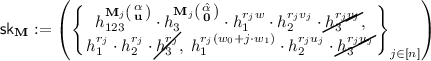
\(\mathsf {KeyGen}(\textsf {mpk},\textsf {msk},\mathbf {M})\): On input a monotone span program \(\mathbf {M}\in \mathbb {Z}_N^{n \times {\ell '}}\), pick \(\mathbf {u}\leftarrow _{\textsc {r}}\mathbb {Z}_N^{{\ell '}-1}\) and \(r_j \leftarrow _{\textsc {r}}\mathbb {Z}_N\) for all \(j \in [n]\), and output
$$ \mathsf {sk}_{\mathbf {M}} := \big ( \, \{\,K_{0,j} := h_{123}^{\mathbf {M}_j\left( {\begin{matrix}\alpha \\ \mathbf {u}\end{matrix}}\right) } \cdot h_1^{ r_j w},\, K_{1,j} := h_{1}^{r_j},\, K_{2,j} := h_{1}^{r_j(w_0+j \cdot w_1)}\;\}_{j\in [n]} \, \big )\in H_N^{3n}. $$ -
\(\mathsf {Dec}(\textsf {mpk}, \mathsf {sk}_{\mathbf {M}}, \mathsf {ct}_{\mathbf {x}})\): If \(\mathbf {x}\) satisfies \(\mathbf {M}\), compute \(\omega _1,\ldots ,\omega _n \in \mathbb {Z}_p\) such that
$$\textstyle \sum _{j : x_j = 1} \omega _j \mathbf {M}_j = \mathbf {1}. $$Then, compute
$$\textstyle K \leftarrow \prod _{j : x_j = 1}\left( e(C_0, K_{0,j}) \cdot e(C_{1,j},K_{1,j})^{-1} \cdot e(C_{2,j},K_{2,j})\right) ^{\omega _j}, $$and recover the message as \(m \leftarrow C/ \mathsf {H}(K) \in \{0,1\}^{\lambda }\).
It is direct to prove the correctness and we omit the detail here.
4.2 Proof of Security
We prove the following theorem:
Theorem 1
Under the subgroup decision assumptions and the subgroup Diffie-Hellman assumptions (cf. Sect. 3.1), the unbounded KP-ABE scheme described in this section (cf. Sect. 4.1) is adaptively secure (cf. Sect. 2.2).
Main Technical Lemma. We prove the following technical lemma. Our proof consists of two steps. We first apply the entropy expansion lemma (see Lemma 2) and obtain a copy of the LOSTW KP-ABE (variant there-of) in the \(p_2\)-subgroup. We may then carry out the classic dual system methodology used for establishing adaptive security of the LOSTW KP-ABE in the \(p_2\)-subgroup with the \(p_3\)-subgroup as the semi-functional space.
Lemma 5
For any adversary \(\mathcal {A}\) that makes at most Q key queries against the unbounded KP-ABE scheme, there exist adversaries \(\mathcal {B}_0,\mathcal {B}_1,\mathcal {B}_2,\mathcal {B}_2\) such that:
where \(\mathsf {Time}(\mathcal {B}_0), \mathsf {Time}(\mathcal {B}_1),\mathsf {Time}(\mathcal {B}_2),\mathsf {Time}(\mathcal {B}_3) \approx \mathsf {Time}(\mathcal {A})\). In particular, we achieve security loss \(O(n+Q)\) based on the \(\text {SD}^{H_N}_{p_{1} \mapsto p_{1}p_{2}}\), \(\text {SD}^{H_N}_{p_{1} \mapsto p_{1}p_{3}}\), \(\text {SD}^{G_N}_{p_{1} \mapsto p_{1}p_{2}}\), \(\text {DDH}^{H_N}_{p_{2}}\), \(\text {SD}^{G_N}_{p_{1} \mapsto p_{1}p_{3}}\), \(\text {DDH}^{H_N}_{p_{3}}\), \(\text {SD}^{G_N}_{p_{3} \mapsto p_{3}p_{2}}\), \(\text {SD}^{G_N}_{p_{2} \mapsto p_{2}p_{3}}\), \(\text {SD}^{H_N}_{p_{2} \mapsto p_{2}p_{3}}\) assumptions.
The proof follows a series of games based on the dual system methodology (see Fig. 4). We first define the auxiliary distributions, upon which we can describe the games.

Game sequence for our composite-order unbounded KP-ABE.
Auxiliary Distributions. We define various forms of a ciphertext (of message m under attribute vector \(\mathbf {x}\)):
-
Normal: Generated by \(\mathsf {Enc}\).
-
E-normal: Same as a normal ciphertext except that a copy of normal ciphertext is created in \(G_{p_2}\) and then we use the substitution:
$$\begin{aligned} w \mapsto v_j \bmod p_2 \text { in }j\text {'th component} \quad \text{ and }\quad w_0 + j \cdot w_1 \mapsto u_j \bmod p_2 \end{aligned}$$(10)where \(v_j,u_j \leftarrow _{\textsc {r}}\mathbb {Z}_N\). Concretely, an E-normal ciphertext is of the form

where \(g_2\) is a random generator of \(G_{p_2}\) and \(s,s_j \leftarrow _{\textsc {r}}\mathbb {Z}_N\).
-
SF: Same as E-normal ciphertext except that we copy all entropy from \(G_{p_2}\) to \(G_{p_3}\). Concretely, an SF ciphertext is of the form
where \(g_3\) is a random generator of \(G_{p_3}\) and \(s,s_j \leftarrow _{\textsc {r}}\mathbb {Z}_N\).


Then we pick \(\hat{\alpha }\leftarrow _{\textsc {r}}\mathbb {Z}_N\) and define various forms of a key (for span program \(\mathbf {M}\)):
-
Normal: Generated by \(\mathsf {KeyGen}\).
-
E-normal: Same as a normal key except that a copy of \(\{h_1^{r_j w},h_1^{r_j},h_1^{r_j(w_0 + j \cdot w_1)}\}_{j\in [n]}\) is created in \(H_{p_2}\) and use the same substitution as in (10). Concretely, an E-normal key is of the form

where \(h_{123}\), \(h_{1}\) and \(h_2\) are respective random generators of \(H_N\), \(H_{p_1}\) and \(H_{p_2}\), \(\mathbf {u}\leftarrow _{\textsc {r}}\mathbb {Z}_N^{{\ell '}-1}\) and \(r_j \leftarrow _{\textsc {r}}\mathbb {Z}_N\).
-
P-normal: Same as E-normal key except that a copy of \(\{h_2^{r_j v_j},h_2^{r_j},h_2^{r_ju_j}\}_{j\in [n]}\) is created in \(H_{p_3}\). Concretely, a P-normal key is of the form

where \(h_{3}\) is a random generator of \(H_{p_3}\), \(\mathbf {u}\leftarrow _{\textsc {r}}\mathbb {Z}_N^{{\ell '}-1}\) and \(r_j \leftarrow _{\textsc {r}}\mathbb {Z}_N\).
-
P-SF: Same as P-normal key except that \(\hat{\alpha }\) is introduced in \(H_{p_3}\). Concretely, a P-SF key is of the form

where \(\mathbf {u}\leftarrow _{\textsc {r}}\mathbb {Z}_N^{{\ell '}-1}\) and \(r_j \leftarrow _{\textsc {r}}\mathbb {Z}_N\).
-
SF: Same as P-SF key except that \(\{h_3^{r_j v_j},h_3^{r_j},h_3^{r_ju_j}\}_{j\in [n]}\) is removed. Concretely, a SF key is of the form
where \(\mathbf {u}\leftarrow _{\textsc {r}}\mathbb {Z}_N^{{\ell '}-1}\) and \(r_j \leftarrow _{\textsc {r}}\mathbb {Z}_N\).


Here E, P, SF means “expanded”, “pesudo”, “semi-functional”, respectively.
Games. We describe the game sequence in detail. For each following claim, we omit its formal proof but provide a proof sketch instead.
\(\underline{\mathsf {Game}_0.}\) The real security game (cf. Sect. 2.2) where keys and ciphertext are normal.
\(\underline{\mathsf {Game}_0'.}\) Identical to \(\mathsf {Game}_0\) except that all keys and the challenge ciphertext are E-normal. We claim that \(\mathsf {Game}_0 \approx _c \mathsf {Game}_{0'}\). This follows from the entropy expansion lemma (see Lemma 2). In the reduction, on input
we select a random generator \(h_{123}\) of \(H_N\), sample \(\alpha \leftarrow _{\textsc {r}}\mathbb {Z}_N\), \(\mathbf {u}_\kappa \leftarrow _{\textsc {r}}\mathbb {Z}_N^{{\ell '}-1}\), \(\tilde{r}_{j,\kappa } \leftarrow _{\textsc {r}}\mathbb {Z}_N\) for \(j\in [n]\) and \(\kappa \in [Q]\), and simulate the game with
\(\underline{\mathsf {Game}_i.}\) Identical to \(\mathsf {Game}_{0'}\) except that the first \(i-1\) keys and the challenge ciphertext is SF. We claim that \(\mathsf {Game}_{0'} \approx _c \mathsf {Game}_1\). This follows from the \(\text {SD}^{G_N}_{p_{2} \mapsto p_{2}p_{3}}\) assumption, which asserts that

In the reduction, we sample \(w,w_0,w_1,v_j,u_j\leftarrow _{\textsc {r}}\mathbb {Z}_N, h_{123}\leftarrow _{\textsc {r}}H_N\), \(\alpha \leftarrow _{\textsc {r}}\mathbb {Z}_N\) and simulate \(\textsf {mpk}, \mathsf {sk}^\kappa _\mathbf {M}\) honestly. To show that \(\mathsf {Game}_i \approx _c \mathsf {Game}_{i+1}\), we will require another sequence of sub-games.
\(\underline{\mathsf {Game}_{i,1}.}\) Identical to \(\mathsf {Game}_i\) except that the i’th key is P-normal. We claim that \(\mathsf {Game}_{i} \approx _c \mathsf {Game}_{i,1}\). This follows from \(\text {SD}^{H_N}_{p_{2} \mapsto p_{2}p_{3}}\) assumption which asserts that
In the reduction, we sample \(w,w_0,w_1,v_j,u_j,\alpha ,\hat{\alpha }\leftarrow _{\textsc {r}}\mathbb {Z}_N\) and select a random generator \(h_{123}\) of \(H_{N}\), and simulate \(\textsf {mpk}, \mathsf {ct},\{ \mathsf {sk}^\kappa _\mathbf {M}\}_{\kappa \ne i}\) honestly.
\(\underline{\mathsf {Game}_{i,2}.}\) Identical to \(\mathsf {Game}_{i}\) except that the i’th key is P-SF. We claim that \(\mathsf {Game}_{i,1} \equiv \mathsf {Game}_{i,2}\). This follows from Lemma 1 in Sect. 2 which ensures that for any \(\mathbf {x}\) that does not satisfy \(\mathbf {M}\),

where \(v_j \leftarrow _{\textsc {r}}\mathbb {Z}_N\) and \(\mathbf {u}\leftarrow _{\textsc {r}}\mathbb {Z}_N^{{\ell '}-1}\), and for all \(\alpha \), \(\hat{\alpha }\), and \(r_j \ne 0 \bmod p_3\). It is straight-forward to compute the remaining terms in \(\textsf {mpk}\), the challenge ciphertext and the Q secret keys by sampling \(g_1,w,w_0,w_1,u_j,s,s_j\) ourselves.
\(\underline{\mathsf {Game}_{i,3}.}\) Identical to \(\mathsf {Game}_{i}\) except that the i’th key is SF. We claim that \(\mathsf {Game}_{i,2} \approx _c \mathsf {Game}_{i,3}\). The proof is completely analogous to that of \(\mathsf {Game}_{i} \approx _c \mathsf {Game}_{i,1}\). Furthermore, observe that \(\mathsf {Game}_{i,3}\) is actually identical to \(\mathsf {Game}_{i+1}\).
\(\underline{\mathsf {Game}_\text {Final}.}\) Identical to \(\mathsf {Game}_{Q+1}\) except that the challenge ciphertext is a SF one for a random message in \(G_T\). We claim that \(\mathsf {Game}_{Q+1} \equiv \mathsf {Game}_\text {Final}\). This follows from the fact that

where \(g_{123}\), \(h_{123}\) and \(h_3\) are respective random generators of \(G_N\), \(H_N\) and \(H_{p_3}\), \(\alpha ,\hat{\alpha }\leftarrow _{\textsc {r}}\mathbb {Z}_N\). The message \(m_b\) is statistically hidden by \(e(g_{123}^s,h_3^{\hat{\alpha }})\). In \(\mathsf {Game}_\text {Final}\), the view of the adversary is statistically independent of the challenge bit b. Hence, \(\mathsf {Adv}_\text {Final}=0\).
5 Simulating Composite-Order Groups in Prime-Order Groups
We build upon and extend the previous framework of Chen et al. [6, 11] for simulating composite-order groups in prime-order ones. We provide prime-order analogues of the static assumptions \(\text {SD}^{G_N}_{p_{1} \mapsto p_{1}p_{2}}, \text {DDH}^{H_N}_{p_{1}}\) used in the previous sections. Moreover, we show that these prime-order analogues follow from the standard k-Linear assumption (and more generally, the MDDH assumption [9]) in prime-order bilinear groups.
Additional Notation. Let \(\mathbf {A}\) be a matrix over \(\mathbb {Z}_p\). We use \(\mathsf {span}(\mathbf {A})\) to denote the column span of \(\mathbf {A}\), and we use \(\mathsf {span}^{\ell }(\mathbf {A})\) to denote matrices of width \(\ell \) where each column lies in \(\mathsf {span}(\mathbf {A})\); this means \(\mathbf {M}\leftarrow _{\textsc {r}}\mathsf {span}^{\ell }(\mathbf {A})\) is a random matrix of width \(\ell \) where each column is chosen uniformly from \(\mathsf {span}(\mathbf {A})\). We use \(\mathsf {basis}(\mathbf {A})\) to denote a basis of \(\mathsf {span}(\mathbf {A})\), and we use \((\mathbf {A}_1 \mid \mathbf {A}_2)\) to denote the concatenation of matrices \(\mathbf {A}_1,\mathbf {A}_2\). If \(\mathbf {A}\) is a m-by-n matrix with \(m > n\), we use \(\overline{\mathbf {A}}\) to denote the sub-matrix consisting of the first n rows and \(\underline{\mathbf {A}}\) the sub-matrix with remaining \(m-n\) rows. We let \(\mathbf {I}_n\) be the n-by-n identity matrix and \(\mathbf {0}\) be a zero matrix whose size will be clear from the context.
5.1 Prime-Order Groups and Matrix Diffie-Hellman Assumptions
A generator \(\mathcal {G}\) takes as input a security parameter \(\lambda \) and outputs a description \(\mathbb {G}:= (p,G_1,G_2,G_T,e)\), where p is a prime of \(\varTheta (\lambda )\) bits, \(G_1\), \(G_2\) and \(G_T\) are cyclic groups of order p, and \(e : G_1 \times G_2 \rightarrow G_T\) is a non-degenerate bilinear map. We require that the group operations in \(G_1\), \(G_2\) and \(G_T\) as well the bilinear map e are computable in deterministic polynomial time with respect to \(\lambda \). Let \(g_1 \in G_1\), \(g_2 \in G_2\) and \(g_T = e(g_1,g_2) \in G_T\) be the respective generators. We employ the implicit representation of group elements: for a matrix \(\mathbf {M}\) over \(\mathbb {Z}_p\), we define \([\mathbf {M}]_1:=g_1^{\mathbf {M}},[\mathbf {M}]_2:=g_2^{\mathbf {M}},[\mathbf {M}]_T:=g_T^{\mathbf {M}}\), where exponentiation is carried out component-wise. Also, given \([\mathbf {A}]_1,[\mathbf {B}]_2\), we let \(e([\mathbf {A}]_1,[\mathbf {B}]_2) = [\mathbf {A}\mathbf {B}]_T\).
We define the matrix Diffie-Hellman (MDDH) assumption on \(G_1\) [9]:
Assumption 3
( \(\mathbf {MDDH}^{m}_{k,\ell }\) Assumption). Let \(\ell > k \ge 1\) and \(m \ge 1\). We say that the \(\text {MDDH}^{m}_{k,\ell }\) assumption holds if for all PPT adversaries \(\mathcal {A}\), the following advantage function is negligible in \(\lambda \).
where \(\mathbf {M}\leftarrow _{\textsc {r}}\mathbb {Z}_p^{\ell \times k}\), \(\mathbf {S}\leftarrow _{\textsc {r}}\mathbb {Z}_p^{k \times m}\) and \(\mathbf {U}\leftarrow _{\textsc {r}}\mathbb {Z}_p^{\ell \times m}\).
The MDDH assumption on \(G_2\) can be defined in an analogous way. Escala et al. [9] showed that
with a tight security reduction. Henceforth, we will use \(\text {MDDH}_{k}\) to denote \(\text {MDDH}_{k,k+1}^1\).
5.2 Basis Structure
We want to simulate composite-order groups whose order is the product of three primes. Fix parameters \(\ell _1,\ell _2,\ell _3, \ell _W \ge 1\). Pick random
where \(\ell := \ell _1 + \ell _2 + \ell _3\). Let \((\mathbf {A}^{\Vert }_1 \mid \mathbf {A}^{\Vert }_2 \mid \mathbf {A}^{\Vert }_3)^{\top }\) denote the inverse of \((\mathbf {A}_1 \mid \mathbf {A}_2 \mid \mathbf {A}_3)\), so that \(\mathbf {A}_i^{\top }\mathbf {A}^{\Vert }_i = \mathbf {I}\) (known as non-degeneracy) and \(\mathbf {A}_i^{\top }\mathbf {A}^{\Vert }_j = \mathbf {0}\) if \(i \ne j\) (known as orthogonality), as depicted in Fig. 5. This generalizes the constructions in [10, 11] where \(\ell _1 = \ell _2 = \ell _3 = k\).

Basis relations. Solid lines mean orthogonal, dashed lines mean non-degeneracy. Similar relations hold in composite-order groups with \((g_1,g_2,g_3)\) in place of \((\mathbf {A}_1,\mathbf {A}_2,\mathbf {A}_3)\) and \((h_1,h_2,h_3)\) in place of \((\mathbf {A}^{\Vert }_1,\mathbf {A}^{\Vert }_2,\mathbf {A}^{\Vert }_3)\).
Correspondence. We have the following correspondence with composite-order groups:
The following statistical lemma is analogous to the Chinese Remainder Theorem, which tells us that \(w \bmod p_2\) is uniformly random given \(g_1^w, g_3^w\), where \(w \leftarrow _{\textsc {r}}\mathbb {Z}_N\):
Lemma 6
(statistical lemma). With probability \(1-1/p\) over \(\mathbf {A}_1,\mathbf {A}_2,\mathbf {A}_3,\mathbf {A}_1^{\parallel },\mathbf {A}_2^{\parallel },\mathbf {A}_3^{\parallel }\), the following two distributions are statistically identical.

where \(\mathbf {W}\leftarrow _{\textsc {r}}\mathbb {Z}_p^{\ell \times \ell _W}\) and \(\mathbf {U}^{(2)} \leftarrow _{\textsc {r}}\mathsf {span}^{\ell _W}(\mathbf {A}^{\Vert }_2)\).
5.3 Basic Assumptions
We first describe the prime-order \((\mathbf {A}_1 \mapsto \mathbf {A}_1,\mathbf {A}_2)\) -subgroup decision assumption, denoted by \(\text {SD}^{G_1}_{\mathbf {A}_{1} \mapsto \mathbf {A}_{1},\mathbf {A}_{2}}\). This is analogous to the subgroup decision assumption in composite-order groups \(\text {SD}^{G_N}_{p_{1} \mapsto p_{1}p_{2}}\) which asserts that \(G_{p_1} \approx _c G_{p_1p_2}\) given \(h_1,h_{3},h_{12}\) along with \(g_1,g_2,g_3\). By symmetry, we can permute the indices for \(\mathbf {A}_1,\mathbf {A}_2,\mathbf {A}_3\).
Lemma 7
( \(\mathbf {MDDH}_{\ell _1,\ell _1+\ell _2} \Rightarrow \mathbf {SD}^{G_1}_{\mathbf {A}_{1} \mapsto \mathbf {A}_{1},\mathbf {A}_{2}}\) ). Under the \(\text {MDDH}_{\ell _1,\ell _1+\ell _2}\) assumption in \(G_1\), there exists an efficient sampler outputting random \(([\mathbf {A}_1]_1,[\mathbf {A}_2]_1,[\mathbf {A}_3]_1)\) (as described in Sect. 5.2) along with base \(\mathsf {basis}(\mathbf {A}^{\Vert }_1)\), \(\mathsf {basis}(\mathbf {A}^{\Vert }_3)\), \(\mathsf {basis}(\mathbf {A}^{\Vert }_1,\mathbf {A}^{\Vert }_2)\) (of arbitrary choice) such that the following advantage function is negligible in \(\lambda \).
where
Similar statements were also implicit in [10, 11].
We then formalize the prime-order \(\mathbf {A}_1\) -subgroup Diffie-Hellman assumption, denoted by \(\text {DDH}^{G_2}_{\mathbf {A}_{1}}\). This is analogous to the subgroup Diffie-Hellman assumption in the composite-order group \(\text {DDH}^{H_N}_{p_{1}}\) which ensures that \(\{ h_{1}^{r_j w}, h_{1}^{r_j} \}_{j\in [Q]} \approx _c \{ h_{1}^{r_j w} \cdot h_1^{u_j}, h_{1}^{r_j}\}_{j\in [Q]}\) given \(g_1,g_2,g_3,h_1,h_2,h_3\) for \(Q = \text{ poly }(\lambda )\). One can permute the indices for \(\mathbf {A}_1,\mathbf {A}_2,\mathbf {A}_3\).
Lemma 8
( \(\mathbf {MDDH}_{\ell _W,Q}^{\ell _1} \Rightarrow \mathbf {DDH}^{G_2}_{\mathbf {A}_{1}}\) ). Fix \(Q = \text{ poly }(\lambda )\) with \(Q>\ell _W\ge 1\). Under the \(\text {MDDH}^{\ell _1}_{\ell _W,Q}\) assumption in \(G_2\), the following advantage function is negligible in \(\lambda \)
where
and \(\mathbf {W}\leftarrow _{\textsc {r}}\mathbb {Z}_p^{\ell \times \ell _W}\), \(\mathbf {D}\leftarrow _{\textsc {r}}\mathbb {Z}_p^{\ell _W \times Q}\), \(\mathbf {R}^{(1)} \leftarrow _{\textsc {r}}\mathsf {span}^{Q}(\mathbf {A}^{\Vert }_1)\).
6 KP-ABE for Monotone Span Programs in Prime-Order Groups
In this section, we present our adaptively secure, unbounded KP-ABE for monotone span programs programs based on the k-Lin assumption in prime-order groups.
6.1 Construction
-
\(\mathsf {Setup}(1^\lambda , 1^n)\): On input \((1^\lambda , 1^n)\), sample \(\mathbf {A}_1 \leftarrow _{\textsc {r}}\mathbb {Z}_p^{(2k+1) \times k}, \mathbf {B}\leftarrow _{\textsc {r}}\mathbb {Z}_p^{(k+1) \times k}\) and
$$ \mathbf {W}, \mathbf {W}_0, \mathbf {W}_1 \leftarrow _{\textsc {r}}\mathbb {Z}_p^{(2k+1) \times (k+1)},\;\mathbf {k}\leftarrow _{\textsc {r}}\mathbb {Z}_p^{2k+1} $$and output the master public and secret key pair
$$\begin{aligned} \textsf {mpk}:=&\left( \; [\mathbf {A}_1^{\top },\mathbf {A}_1^{\top }\mathbf {W},\mathbf {A}_1^{\top }\mathbf {W}_0,\mathbf {A}_1^{\top }\mathbf {W}_1]_1,\; e([\mathbf {A}_1^{\top }]_1, [\mathbf {k}]_2) \;\right) \\ \textsf {msk}:=&\left( \;\mathbf {k},\;\mathbf {B},\; \mathbf {W},\;\mathbf {W}_0,\;\mathbf {W}_1 \;\right) . \end{aligned}$$ -
\(\mathsf {Enc}(\textsf {mpk},\mathbf {x},m)\): On input an attribute vector \(\mathbf {x}:=(x_1,\ldots ,x_n)\in \{0,1\}^n\) and \(m \in G_T\), pick \(\mathbf {c},\mathbf {c}_j\leftarrow _{\textsc {r}}\mathsf {span}(\mathbf {A}_1)\) for all \(j \in [n]\) and output
$$\begin{aligned} \begin{array}{cc} \mathsf {ct}_{\mathbf {x}}:=\left( \begin{array}{l} C_0 := [\mathbf {c}^{\top }]_{1},\\ \{\;C_{1,j} :=[\mathbf {c}^{\top }\mathbf {W}+ \mathbf {c}_j^{\top }(\mathbf {W}_0 + j \cdot \mathbf {W}_1)]_{1}, C_{2,j} :=[\mathbf {c}_j^{\top }]_{1}\;\}_{j:x_j=1}, \\ C := e([\mathbf {c}^{\top }]_1,[\mathbf {k}]_2) \cdot m \end{array}\right) \\ \in G_1^{2k+1} \times (G_1^{k+1} \times G_1^{2k+1})^{n}\times G_T. \end{array} \end{aligned}$$ -
\(\mathsf {KeyGen}(\textsf {mpk},\textsf {msk},\mathbf {M})\): On input a monotone span program \(\mathbf {M}\in \mathbb {Z}_p^{n\times {\ell '}}\), pick \(\mathbf {K}'\leftarrow _{\textsc {r}}\mathbb {Z}_p^{ (2k+1)\times ({\ell '}-1)}\), \( \mathbf {d}_j \leftarrow _{\textsc {r}}\mathsf {span}(\mathbf {B})\) for all \(j \in [n]\), and output
$$\begin{aligned} \begin{array}{c} \mathsf {sk}_{\mathbf {M}} := \left( \left\{ \begin{array}{c} K_{0,j} :=[(\mathbf {k}\Vert \mathbf {K}')\mathbf {M}_j^{\top }+\mathbf {W}\mathbf {d}_j]_{2},\; K_{1,j} := [\mathbf {d}_j]_{2},\\ K_{2,j} := [(\mathbf {W}_0 + j\cdot \mathbf {W}_1) \mathbf {d}_j]_{2} \end{array} \right\} _{j\in [n]} \right) \\ \in (G_2^{2k+1}\times G_2^{k+1} \times G_2^{2k+1})^n. \end{array} \end{aligned}$$ -
\(\mathsf {Dec}(\textsf {mpk}, \mathsf {sk}_{\mathbf {M}}, \mathsf {ct}_{\mathbf {x}})\): If \(\mathbf {x}\) satisfies \(\mathbf {M}\), compute \(\omega _1,\ldots ,\omega _n \in \mathbb {Z}_p\) such that
$$\textstyle \sum _{j : x_j = 1} \omega _j \mathbf {M}_j = \mathbf {1}. $$Then, compute
$$\textstyle K \leftarrow \prod _{j : x_j = 1}\left( e(C_0, K_{0,j}) \cdot e(C_{1,j},K_{1,j})^{-1} \cdot e(C_{2,j},K_{2,j})\right) ^{\omega _j}, $$and recover the message as \(m \leftarrow C/K \in G_T\).
The proof of correctness is direct and we omit it here.
6.2 Entropy Expansion Lemma in Prime-Order Groups
With \(\mathbf {A}_1,\mathbf {A}_2,\mathbf {A}_3,\mathbf {A}^{\Vert }_1,\mathbf {A}^{\Vert }_2,\mathbf {A}^{\Vert }_3\) defined as in Sect. 5.2, our prime-order entropy expansion lemma is stated as follows. The proof is analogous to that for composite-order entropy expansion lemma (Lemma 2) shown in Sect. 3.2.
Lemma 9
(prime-order entropy expansion lemma). Suppose \(\ell _1,\ell _3,\ell _W \ge k\). Then, under the \(\text {MDDH}_{k}\) assumption, we have

where \(\mathbf {W}, \mathbf {W}_0, \mathbf {W}_1 \leftarrow _{\textsc {r}}\mathbb {Z}_p^{\ell \times {\ell _W}}, \mathbf {V}^{(2)}_j,\mathbf {U}^{(2)}_j \leftarrow _{\textsc {r}}\mathsf {span}^{{\ell _W}}(\mathbf {A}_2^{\parallel }),\mathbf {D}_{j} \leftarrow _{\textsc {r}}\mathbb {Z}_p^{{\ell _W}\times {\ell _W}}\), and \(\mathbf {c},\mathbf {c}_j \leftarrow _{\textsc {r}}\mathsf {span}(\mathbf {A}_1)\) in the left distribution while \(\mathbf {c},\mathbf {c}_j\leftarrow _{\textsc {r}}\mathsf {span}(\mathbf {A}_1,\mathbf {A}_2)\) in the right distribution. Concretely, the distinguishing advantage \(\mathsf {Adv}^{\textsc {ExpLem}}_{{\mathcal {A}}}(\lambda )\) is at most
where \(\mathsf {Time}(\mathcal {B})\), \(\mathsf {Time}(\mathcal {B}_0)\), \(\mathsf {Time}(\mathcal {B}_1)\), \(\mathsf {Time}(\mathcal {B}_2)\), \(\mathsf {Time}(\mathcal {B}_4)\), \(\mathsf {Time}(\mathcal {B}_6)\), \(\mathsf {Time}(\mathcal {B}_7)\), \(\mathsf {Time}(\mathcal {B}_8) \approx \mathsf {Time}(\mathcal {A})\).
Remark 1
(Differences from overview in Sect. 1.3 ). We stated our prime-order expansion lemma for general \(\ell _1,\ell _2,\ell _3\); for our KP-ABE, it suffices to set \((\ell _1,\ell _2,\ell _3) = (k,1,k)\). Compared to the informal statement (8) in Sect. 1.3, we use \(\mathbf {A}_2 \in \mathbb {Z}_p^{2k+1}\) instead of \(\mathbf {A}_2 \in \mathbb {Z}_p^{(2k+1) \times k}\), and we introduced extra \(\mathbf {A}_2\)-components corresponding to \(\mathbf {A}_2^{\top }\mathbf {W}, \mathbf {A}_2^{\top }(\mathbf {W}_0 + j \cdot \mathbf {W}_1)\) in \( \mathsf {ct}\) on the RHS. We have \(\mathbf {D}_j\) in place of \(\mathbf {B}\mathbf {r}_j\) in the above statement, though we will introduce \(\mathbf {B}\) later on in Lemma 10. We also picked \(\mathbf {D}_{j}\) to be square matrices to enable random self-reducibility of the \( \mathsf {sk}\)-terms. Finally, \(\mathbf {V}^{(2)}_j,\mathbf {U}^{(2)}_j\) correspond to \(\mathbf {V}_j,\mathbf {U}_j\) in the informal statement, and in particular, we have \(\mathbf {A}_1^{\top }\mathbf {V}^{(2)}_j = \mathbf {A}_1^{\top }\mathbf {U}^{(2)}_j = \mathbf {0}\).
6.3 Proof of Security
We prove the following theorem:
Theorem 2
Under the \(\text {MDDH}_{k}\) assumption in prime-order groups (cf. Sect. 5.1), the unbounded KP-ABE scheme for monotone span programs described in this Section (cf. Sect. 6.1) is adaptively secure (cf. Sect. 2.2).
Bilinear Entropy Expansion Lemma, Revisited. With the additional basis \(\mathbf {B}\in \mathbb {Z}_p^{(k+1) \times k}\), we need a variant of the entropy expansion lemma in Lemma 9 with \((\ell _1,\ell _2,\ell _3,\ell _W) = (k,1,k,k+1)\) where the columns of \(\mathbf {D}_j\) are drawn from \(\mathsf {span}(\mathbf {B})\) instead of \(\mathbb {Z}_p^{k+1}\) (see Lemma 10).
Lemma 10
(prime-order entropy expansion lemma, revisited). Pick \((\mathbf {A}_1,\mathbf {a}_2,\mathbf {A}_3)\leftarrow _{\textsc {r}}\mathbb {Z}_p^{(2k+1)\times (k+1)}\times \mathbb {Z}_p^{2k+1}\times \mathbb {Z}_p^{(2k+1)\times (k+1)}\) and define its dual \((\mathbf {A}_1^{\parallel },\mathbf {a}_2^{\parallel },\mathbf {A}_3^{\parallel })\) as in Sect. 5.2. With \(\mathbf {B}\leftarrow _{\textsc {r}}\mathbb {Z}_p^{(k+1) \times k}\), we have

where \(\mathbf {W}, \mathbf {W}_0, \mathbf {W}_1 \leftarrow _{\textsc {r}}\mathbb {Z}_p^{(2k+1) \times (k+1)},\ \mathbf {V}^{(2)}_j,\mathbf {U}^{(2)}_j \leftarrow _{\textsc {r}}\mathsf {span}^{k+1}(\mathbf {a}_2^{\parallel }),\ {\mathbf {D}_{j} \leftarrow _{\textsc {r}}\mathsf {span}^{k+1}(\mathbf {B})}\), and \(\mathbf {c},\mathbf {c}_j \leftarrow _{\textsc {r}}\mathsf {span}(\mathbf {A}_1)\) in the left distribution while \(\mathbf {c},\mathbf {c}_j\leftarrow _{\textsc {r}}\mathsf {span}(\mathbf {A}_1,\mathbf {a}_2)\) in the right distribution. We let \(\mathsf {Adv}^{\textsc {ExpLemRev}}_{{\mathcal {A}}}(\lambda )\) denote the distinguishing advantage.
We claim that the lemma follows from the basic entropy expansion lemma (Lemma 9) and the \(\text {MDDH}_{k}\) assumption, which tells us that
Concretely, for all \(\mathcal {A}\), we can construct \(\mathcal {B}_0\) and \(\mathcal {B}_1\) with \(\mathsf {Time}(\mathcal {B}_0),\mathsf {Time}(\mathcal {B}_1) \approx \mathsf {Time}(\mathcal {A})\) such that
The proof is straight-forward by demonstrating that the left (resp. right) distributions in Lemmas 9 and 10 are indistinguishable under the \(\text {MDDH}_{k}\) assumption and then applying Lemma 9. In the reduction, we sample \(\mathbf {W}, \mathbf {W}_0, \mathbf {W}_1 \leftarrow _{\textsc {r}}\mathbb {Z}_p^{(2k+1) \times (k+1)}\) (and \(\mathbf {V}^{(2)}_j,\mathbf {U}^{(2)}_j \leftarrow _{\textsc {r}}\mathsf {span}^{k+1}(\mathbf {a}_2^{\parallel })\) for the right distributions) and simulate \(\mathsf {aux}, \mathsf {ct}\) honestly.
Main Technical Lemma. We prove the following technical lemma. As with the composite-order scheme in Sect. 4, we first apply the new entropy expansion lemma in Lemma 10 and obtain a copy of the CGW KP-ABE (variant-thereof) in the \(\mathbf {a}_2\)-subspace. We may then carry out the classic dual system methodology used for establishing adaptive security of the CGW KP-ABE.
Lemma 11
For any adversary \(\mathcal {A}\) that makes at most Q key queries against the unbounded KP-ABE scheme, there exist adversaries \(\mathcal {B}_0,\mathcal {B}_1,\mathcal {B}_2\) such that:
where \(\mathsf {Time}(\mathcal {B}_0), \mathsf {Time}(\mathcal {B}_1), \mathsf {Time}(\mathcal {B}_2) \approx \mathsf {Time}(\mathcal {A})\). In particular, we achieve security loss \(O(n+Q)\) based on the \(\text {MDDH}_{k}\) assumption.
The proof follows the same game sequence as shown in Sect. 4.2 except that the adversary is given an E-normal challenge ciphertext instead of a SF one in \(\mathsf {Game}_i\), \(\mathsf {Game}_{i,1}\), \(\mathsf {Game}_{i,2}\), \(\mathsf {Game}_{i,3}\) (in fact, we do not need to define SF ciphertexts) and the auxiliary distributions are defined as follows.
Auxiliary Distributions. We define various forms of ciphertext (of message m under attribute vector \(\mathbf {x}\)):
-
Normal: Generated by \(\mathsf {Enc}\); in particular, \(\mathbf {c},\mathbf {c}_j\leftarrow _{\textsc {r}}\mathsf {span}(\mathbf {A}_1)\).
-
E-normal: Same as a normal ciphertext except that \(\mathbf {c},\mathbf {c}_j\leftarrow _{\textsc {r}}\mathsf {span}(\mathbf {A}_1,\mathbf {a}_2)\) and we use the substitution:
$$\begin{aligned}&\mathbf {W}\mapsto \mathbf {W}+ \mathbf {V}^{(2)}_j \quad \text { in}\,\, j\text {'th component} \nonumber \\ \quad \text{ and }\quad&\mathbf {W}_0 + j \cdot \mathbf {W}_1 \mapsto \mathbf {W}_0 + j \cdot \mathbf {W}_1 + \mathbf {U}^{(2)}_j \end{aligned}$$(11)where \(\mathbf {U}^{(2)}_j,\mathbf {V}^{(2)}_j \leftarrow _{\textsc {r}}\mathsf {span}^{k+1}(\mathbf {a}_2^{\parallel })\).
Then we pick \(\alpha \leftarrow _{\textsc {r}}\mathbb {Z}_p\) and define various forms of key (for span program \(\mathbf {M}\)):
-
Normal: Generated by \(\mathsf {KeyGen}\).
-
E-normal: Same as a normal key except that we use the same substitution as in (11).
-
P-normal: Sample \(\mathbf {d}_j \leftarrow _{\textsc {r}}\mathbb {Z}_p^{k+1}\) in an E-normal key.
-
P-SF: Replace \(\mathbf {k}\) with \(\mathbf {k}+ \alpha \mathbf {a}_2^{\parallel }\) in a P-normal key.
-
SF: Sample \(\mathbf {d}_j \leftarrow _{\textsc {r}}\mathsf {span}(\mathbf {B})\) in a P-SF key.
Notes
- 1.
Some works associate ciphertexts with a set \(S \subseteq [n]\) where [n] is referred to as the attribute universe, in which case \(\mathbf {x}\in \{0,1\}^n\) corresponds to the characteristic vector of S.
- 2.
- 3.
Attrapadung’s unbounded KP-ABE does have the advantage that there is no read-once restriction on the span programs, but even with the read-once restriction, the proof still requires q-type assumptions.
- 4.
And a subgroup assumption to introduce the \(h_2^{\alpha _j}\)’s.
- 5.
With two main differences: (i) we are in the selective setting which allows for a much simpler proof, (ii) we allow \(j = i\) in \( \mathsf {sk}\).
References
Agrawal, S., Chase, M.: FAME: fast attribute-based message encryption. In: ACM CCS (2017)
Attrapadung, N.: Dual system encryption via doubly selective security: framework, fully secure functional encryption for regular languages, and more. In: Nguyen, P.Q., Oswald, E. (eds.) EUROCRYPT 2014. LNCS, vol. 8441, pp. 557–577. Springer, Heidelberg (2014). https://doi.org/10.1007/978-3-642-55220-5_31
Attrapadung, N.: Dual system encryption framework in prime-order groups via computational pair encodings. In: Cheon, J.H., Takagi, T. (eds.) ASIACRYPT 2016, Part II. LNCS, vol. 10032, pp. 591–623. Springer, Heidelberg (2016). https://doi.org/10.1007/978-3-662-53890-6_20
Beimel, A.: Secure Schemes for Secret Sharing and Key Distribution. Ph.D., Technion - Israel Institute of Technology (1996)
Brakerski, Z., Vaikuntanathan, V.: Circuit-ABE from LWE: unbounded attributes and semi-adaptive security. In: Robshaw, M., Katz, J. (eds.) CRYPTO 2016, Part III. LNCS, vol. 9816, pp. 363–384. Springer, Heidelberg (2016). https://doi.org/10.1007/978-3-662-53015-3_13
Chen, J., Gay, R., Wee, H.: Improved dual system ABE in prime-order groups via predicate encodings. In: Oswald, E., Fischlin, M. (eds.) EUROCRYPT 2015, Part II. LNCS, vol. 9057, pp. 595–624. Springer, Heidelberg (2015). https://doi.org/10.1007/978-3-662-46803-6_20
Chen, J., Wee, H.: Fully, (Almost) tightly secure IBE and dual system groups. In: Canetti, R., Garay, J.A. (eds.) CRYPTO 2013, Part II. LNCS, vol. 8043, pp. 435–460. Springer, Heidelberg (2013). https://doi.org/10.1007/978-3-642-40084-1_25
Chen, J., Wee, H.: Semi-adaptive attribute-based encryption and improved delegation for boolean formula. In: Abdalla, M., De Prisco, R. (eds.) SCN 2014. LNCS, vol. 8642, pp. 277–297. Springer, Cham (2014). https://doi.org/10.1007/978-3-319-10879-7_16
Escala, A., Herold, G., Kiltz, E., Ràfols, C., Villar, J.: An algebraic framework for Diffie-Hellman assumptions. In: Canetti, R., Garay, J.A. (eds.) CRYPTO 2013, Part II. LNCS, vol. 8043, pp. 129–147. Springer, Heidelberg (2013). https://doi.org/10.1007/978-3-642-40084-1_8
Gay, R., Hofheinz, D., Kiltz, E., Wee, H.: Tightly CCA-secure encryption without pairings. In: Fischlin, M., Coron, J.-S. (eds.) EUROCRYPT 2016, Part I. LNCS, vol. 9665, pp. 1–27. Springer, Heidelberg (2016). https://doi.org/10.1007/978-3-662-49890-3_1
Gong, J., Dong, X., Chen, J., Cao, Z.: Efficient IBE with tight reduction to standard assumption in the multi-challenge setting. In: Cheon, J.H., Takagi, T. (eds.) ASIACRYPT 2016, Part II. LNCS, vol. 10032, pp. 624–654. Springer, Heidelberg (2016). https://doi.org/10.1007/978-3-662-53890-6_21
Goyal, R., Koppula, V., Waters, B.: Semi-adaptive security and bundling functionalities made generic and easy. In: Hirt, M., Smith, A. (eds.) TCC 2016, Part II. LNCS, vol. 9986, pp. 361–388. Springer, Heidelberg (2016). https://doi.org/10.1007/978-3-662-53644-5_14
Goyal, V., Pandey, O., Sahai, A., Waters, B.: Attribute-based encryption for fine-grained access control of encrypted data. In: Juels, A., Wright, R.N., Vimercati, S. (eds.) ACM CCS 2006, pp. 89–98. ACM Press, October/November 2006. Available as Cryptology ePrint Archive Report 2006/309
Hofheinz, D., Jager, T., Knapp, E.: Waters signatures with optimal security reduction. In: Fischlin, M., Buchmann, J., Manulis, M. (eds.) PKC 2012. LNCS, vol. 7293, pp. 66–83. Springer, Heidelberg (2012). https://doi.org/10.1007/978-3-642-30057-8_5
Ishai, Y., Wee, H.: Partial garbling schemes and their applications. In: Esparza, J., Fraigniaud, P., Husfeldt, T., Koutsoupias, E. (eds.) ICALP 2014, Part I. LNCS, vol. 8572, pp. 650–662. Springer, Heidelberg (2014). https://doi.org/10.1007/978-3-662-43948-7_54
Karchmer, M., Wigderson, A.: On span programs. In: Structure in Complexity Theory Conference, pp. 102–111 (1993)
Kowalczyk, L., Lewko, A.B.: Bilinear entropy expansion from the decisional linear assumption. In: Gennaro, R., Robshaw, M. (eds.) CRYPTO 2015, Part II. LNCS, vol. 9216, pp. 524–541. Springer, Heidelberg (2015). https://doi.org/10.1007/978-3-662-48000-7_26
Lewko, A.: Tools for simulating features of composite order bilinear groups in the prime order setting. In: Pointcheval, D., Johansson, T. (eds.) EUROCRYPT 2012. LNCS, vol. 7237, pp. 318–335. Springer, Heidelberg (2012). https://doi.org/10.1007/978-3-642-29011-4_20
Lewko, A., Okamoto, T., Sahai, A., Takashima, K., Waters, B.: Fully secure functional encryption: attribute-based encryption and (hierarchical) inner product encryption. In: Gilbert, H. (ed.) EUROCRYPT 2010. LNCS, vol. 6110, pp. 62–91. Springer, Heidelberg (2010). https://doi.org/10.1007/978-3-642-13190-5_4
Lewko, A., Waters, B.: New techniques for dual system encryption and fully secure HIBE with short ciphertexts. In: Micciancio, D. (ed.) TCC 2010. LNCS, vol. 5978, pp. 455–479. Springer, Heidelberg (2010). https://doi.org/10.1007/978-3-642-11799-2_27
Lewko, A., Waters, B.: Unbounded HIBE and attribute-based encryption. In: Paterson, K.G. (ed.) EUROCRYPT 2011. LNCS, vol. 6632, pp. 547–567. Springer, Heidelberg (2011). https://doi.org/10.1007/978-3-642-20465-4_30
Okamoto, T., Takashima, K.: Fully secure functional encryption with general relations from the decisional linear assumption. In: Rabin, T. (ed.) CRYPTO 2010. LNCS, vol. 6223, pp. 191–208. Springer, Heidelberg (2010). https://doi.org/10.1007/978-3-642-14623-7_11
Okamoto, T., Takashima, K.: Fully secure unbounded inner-product and attribute-based encryption. In: Wang, X., Sako, K. (eds.) ASIACRYPT 2012. LNCS, vol. 7658, pp. 349–366. Springer, Heidelberg (2012). https://doi.org/10.1007/978-3-642-34961-4_22
Rouselakis, Y., Waters, B.: Practical constructions and new proof methods for large universe attribute-based encryption. In: Sadeghi, A.-R., Gligor, V.D., Yung, M. (eds.) ACM CCS 2013, pp. 463–474. ACM Press, November 2013
Sahai, A., Waters, B.: Fuzzy identity-based encryption. In: Cramer, R. (ed.) EUROCRYPT 2005. LNCS, vol. 3494, pp. 457–473. Springer, Heidelberg (2005). https://doi.org/10.1007/11426639_27
Waters, B.: Dual system encryption: realizing fully secure IBE and HIBE under simple assumptions. In: Halevi, S. (ed.) CRYPTO 2009. LNCS, vol. 5677, pp. 619–636. Springer, Heidelberg (2009). https://doi.org/10.1007/978-3-642-03356-8_36
Wee, H.: Dual system encryption via predicate encodings. In: Lindell, Y. (ed.) TCC 2014. LNCS, vol. 8349, pp. 616–637. Springer, Heidelberg (2014). https://doi.org/10.1007/978-3-642-54242-8_26
Acknowledgments
We greatly thank Katsuyuki Takashima for insightful and constructive feedback. We also thank all anonymous reviewers for their helpful comments.
Author information
Authors and Affiliations
Corresponding author
Editor information
Editors and Affiliations
Rights and permissions
Copyright information
© 2018 International Association for Cryptologic Research
About this paper

Cite this paper
Chen, J., Gong, J., Kowalczyk, L., Wee, H. (2018). Unbounded ABE via Bilinear Entropy Expansion, Revisited. In: Nielsen, J., Rijmen, V. (eds) Advances in Cryptology – EUROCRYPT 2018. EUROCRYPT 2018. Lecture Notes in Computer Science(), vol 10820. Springer, Cham. https://doi.org/10.1007/978-3-319-78381-9_19
Download citation
DOI: https://doi.org/10.1007/978-3-319-78381-9_19
Published:
Publisher Name: Springer, Cham
Print ISBN: 978-3-319-78380-2
Online ISBN: 978-3-319-78381-9
eBook Packages: Computer ScienceComputer Science (R0)
